Cooperative Localization Algorithm for Multiple Mobile Robot System in Indoor Environment Based on Variance Component Estimation

Abstract

The Multiple Mobile Robot (MMR) cooperative system is becoming a focus of study in various fields due to its advantages, such as high efficiency and good fault tolerance. However, the uncertainty and nonlinearity problems severely limit the cooperative localization accuracy of the MMR system. Thus, to solve the problems mentioned above, this manuscript presents a cooperative localization algorithm for MMR systems based on Cubature Kalman Filter (CKF) and adaptive Variance Component Estimation (VCE) methods. In this novel algorithm, a nonlinear filter named CKF is used to enhance the cooperative localization accuracy and reduce the computational load. On the other hand, the adaptive VCE method is introduced to eliminate the effects of unknown system noise. Furthermore, the performance of the proposed algorithm is compared with that of the cooperative localization algorithm based on normal CKF by utilizing the real experiment data. In addition, the results demonstrate that the proposed algorithm outperforms the CKF cooperative localization algorithm both in accuracy and consistency.

1. Introduction

In recent years, with the development of robot technology, network communication technology and automatic control technology, the Multiple Mobile Robot (MMR) cooperative system has attracted the attention of many researchers. Using multiple mobile robots to execute the task, the MMR cooperative system can not only enhance operation efficiency but also improve the capability of fault tolerance and reconfiguration. Therefore, the MMR cooperative system has shown broad application prospects and is becoming a focus of study in various fields, such as the military, space exploration, traffic control, medical and service trades [1,2].

Exactly knowing the position, velocity, attitude and other motion information of each mobile robot is one of the basic premises of the MMR cooperative system [3,4]. This means that it requires the ability of self-localization for each mobile robot. The MMR cooperative system could achieve the goal of localization by each mobile robot separately and the localization accuracy just depends on the accuracy of the navigation system that is equipped on each mobile robot. Although this kind of localization scheme is simple to achieve, the localization accuracy is limited by the insufficiency of information sharing [5,6]. The relative range or relative bearing between different mobile robots, observed by binocular cameras, monocular cameras or other kinds of sensors, is exchanged among the mobile robot group [1,7]. In addition, the performance of this kind of navigation scheme, which is called cooperative navigation, is superior to the one of the separate navigation scheme [8,9]. In a cooperative navigation system, the performance of a low accuracy navigation system will be improved significantly by utilizing the navigation information from a high accuracy navigation system [10,11]. Furthermore, when some mobile robots lose their capacity of self-localization, the cooperative navigation will help them to recover it [12]. Since the cooperative navigation has so many potential advantages in robotics, it is becoming a key research direction.

The cooperative navigation algorithm is the core and infrastructure of cooperative navigation [13,14]. Typically, the structure of a cooperative navigation algorithm can be implemented in the central centralized manner [15] or the distributed manner [16]. In the centralized manner, all measurement data are collected and processed in a central agent. In addition, in the distributed manner, each agent exchanges information with its neighbors and estimates its own position by itself. Taking computational cost, survivability, and reliability into account, the distributed manner is superior to the centralized manner [17,18].

1.1. Problem Statements

A cooperative navigation algorithm is essentially a data fusion technique that is used to estimate the pose of each mobile robot by utilizing the output of the sensors equipped on each mobile robot. Due to the characteristics of the nonlinearity of MMR systems, nonlinear estimation methods, such as the extended Kalman filter (EKF) and the unscented Kalman filter (UKF), have proven to be effective methods for MMR cooperative localization problems. In the EKF, the nonlinear system can be linearized utilizing the Taylor series expansion for variance propagation, while the prediction of the state vector and measurement vector are conducted using the nonlinear system. Although EKF has been used in many MMR cooperative localization systems for its simplicity, the precision is limited in the systems with strong nonlinearity and the fussy Jacobian matrix should be calculated, which will inevitably increase the computational load. With the Unscented Transformation (UT), the UKF method can approximate the mean and the variance of the Gaussian state distribution using the nonlinear function, avoiding the local linearization and calculation of the Jacobian matrix effectively. However, the covariance matrix sometimes is easily non-positive in high-dimensional systems, which will lead to filtering divergence.

In addition, the above nonlinear filters are optimal only when the mathematical model is exactly known and system noises are of white Gaussian type. However, in actual MMR systems, the measurement noise is not white Gaussian noise. For example, the noise is quantitative in a vision-based MMR system, which is caused by the limited resolution and is relative to distance between the depth from the viewpoint. In [19], the authors separated the measurement depths into different segments according to the quantized measurement error of stereo vision camera firstly. For each segment, the measurement error is modeled as a combination of a fixed constant error and white Gaussian noise. Finally, an adaptive EKF is established, taking the measurement error segment into consideration. Moreover, the experiment result illustrated the effectiveness of the proposed algorithm. However, the key problem of this method is that the quantized measurement error model of the camera should be known as priori knowledge and the quantized error needs accurate calibration before operation. For actual MMR systems, this is difficult to satisfy because of the vast workload. It is well known that the adaptive filter can be utilized to estimate and correct the model parameters and the noise characteristics at the same time [20]. As a result, the adaptive filter has been considered to enhance the estimation accuracy in robotics [21,22]. A Sage–Husa adaptive filter is an outstanding adaptive filter method that is widely used to estimate the variance matrices of the process and measurement noises [23]. Nevertheless, it cannot estimate these two variance matrices simultaneously, which means that one of them should be known as prior knowledge. By adjusting or restraining the impacts of the current observations on the parameter estimation using the fading factor, an adaptive filter makes full use of the current observations to improve the filtering accuracy [24]. However, it is difficult to obtain the optimal fading factor, and the computational complexity will accordingly be increased as well. Furthermore, the weights of the a priori reliable information would be decreased to a certain extent if the current observation is abnormal, and then the filtering accuracy would also be degraded.

1.2. Contributions

By taking the high dimensionality, nonlinearity and the colored measurement noise into account, a novel cooperative localization algorithm is proposed in this paper based on an adaptive CKF method. In order to overcome the influence on cooperative localization accuracy caused by the nonlinearity and high-dimension, the Cubature Kalman filter (CKF) [25,26] is used in the novel algorithm. CKF is based on the Cubature Transform to conduct the prediction using the Cubature points that have the same weight. It has better performance compared with EKF and UKF, especially for the high-dimensional and strong nonlinear system [25,26]. Moreover, in order to overcome the influence on cooperative localization accuracy caused by the uncertainty of measurement noise, the Variance-Covariance Components Estimation (VCE) is used to estimate the noise adaptively [27,28]. At present, various adaptive and robust estimations have been widely used in statistics and geodesy. In addition, one of the famous methods is an a posteriori VCE method on the basis of Helmert, in which the weights of different observations can be calculated by the adaptive iteration. Since the matrix will be negative sometimes during the calculation, some improved methods were proposed. Wang et al. proposed an adaptive Kalman filter (AKF) based on the VCE method, and verified its effectiveness using the actual experiments [27,29]. The state estimation algorithm based on VCE has many advantages and has been widely used in linear systems, but few researchers have applied VCE to nonlinear systems. Since the novel algorithm cannot only estimate the statistical property of the system’s noise, but also be applied in nonlinear MMR systems, the cooperative localization accuracy could be further improved by utilizing the novel algorithm.

The rest is organized as follows. In Section 2, the system model and CKF algorithm are formulated. In Section 3, a novel cooperative localization algorithm based on CKF and VCE is presented. The experiment results are presented in Section 4 and the conclusions are drawn in Section 5.

2. Basic Knowledge

2.1. Nonlinear Model of MMR Cooperative Localization System

2.1.1. State Model

The state model equation of n mobile robots system can be expressed as

$$\mathit{x}={\left[{\mathit{x}}_1,{\mathit{x}}_2,\dots ,{\mathit{x}}_n\right]}^{\top },$$

(1)

where ${\mathit{x}}_i={\left[x_i,y_i,{\theta }_i\right]}^{\top }$ represents the pose of the i-th mobile robot in the MMR group, and it can be expressed as

$$\left\{\begin{array}{c}{x}_i\left(k+1\right)=x_i\left(k\right)+v_i\left(k\right)·cos{\theta }_i\left(k\right),\\ y_i\left(k+1\right)=y_i\left(k\right)+v_i\left(k\right)·sin{\theta }_i\left(k\right),\\ {\theta }_i\left(k+1\right)={\theta }_i\left(k\right)+{\omega }_i\left(k\right).\end{array}\right.$$

(2)

2.1.2. Observation Model

In an MMR system, the bearing and range measurement information is used as the observation and the observation equations are represented as

$$\mathit{z}\left(k\right)={\left[r_{ij},{\varphi }_{ij}\right]}^{\top },$$

(3)

if mobile robot i measures the range and bearing relative to mobile robot j or

$$\mathit{z}\left(k\right)={\left[r_{ik},{\varphi }_{ik}\right]}^{\top },$$

(4)

if mobile robot i measures the range and bearing relative to landmark k, where

$$\left\{\begin{array}{c}tan\left({\theta }_i+{\varphi }_{ij}\right)=\frac{x_i-x_j}{y_i-y_j}\\ r_{ij}=\sqrt{{\left(x_i-x_j\right)}^2+{\left(y_i-y_j\right)}^2},\end{array}\right.$$

(5)

$$\left\{\begin{array}{c}tan\left({\theta }_i+{\varphi }_{ik}\right)=\frac{x_i-x_k}{y_i-y_k}\\ r_{ik}=\sqrt{{\left(x_i-x_k\right)}^2+{\left(y_i-y_k\right)}^2},\end{array}\right.$$

(6)

where Equation (5) represents the observation equation if the mobile robot measures the relative range and bearing relative to another mobile robot, while Equation (6) represents the observation equation if the mobile robot measures the relative range and bearing relative to landmarks; ${\left[x_i,y_i,{\theta }_i\right]}^{\top }$ and ${\left[x_j,y_j,{\theta }_j\right]}^{\top }$ represent the poses of the i-th mobile robot and the j-th mobile robot, respectively; $(x_k,y_k)$ represents the position of k-th landmark.

2.2. MMR Cooperative Localization Algorithm Based on CKF

2.2.1. Structure of MMR Cooperative Localization

Without a loss of generality, it is usually assumed that state transitions and observations occur in alternating order, i.e., after each state transition from $\mathit{x}(k-1)$ to $\mathit{x}\left(k\right)$ an observation $\mathit{z}\left(k\right)$ is recorded. However, the observation information cannot be obtained at each time index for mobile robot systems because of the occlusion. As a result, the cooperative localization algorithm under the framework of an extended Kalman filter is re-established as Algorithm 1. In Algorithm 1, the measurement update is carried out only when measurement information exists. Otherwise, the predicted state estimate and covariance estimate act as the updated state estimate and covariance estimate, respectively.

Algorithm 1 Cooperative localization of MMR

Require:  ${\mathit{P}}_i(k-1,k-1),{\widehat{\mathit{x}}}_i(k-1,k-1)$ Ensure:  ${\mathit{P}}_i(k,k),{\widehat{\mathit{x}}}_i(k,k)$ 1: for $k=1\to n$ do 2:  ${\widehat{\mathit{x}}}_i(k,k-1)\leftarrow \mathit{f}\left[{\widehat{\mathit{x}}}_i(k-1,k-1)\right]$ 3:  ${\widehat{\mathit{P}}}_i(k,k-1)\leftarrow {\mathit{F}}_i\left(k\right){\mathit{P}}_i(k-1,k-1){\mathit{F}}_i{\left(k\right)}^{\top }+{\mathit{Q}}_i\left(k\right)$ 4:  if Obs $=1$ then 5:   ${\tilde{\mathit{y}}}_i\left(k\right)={\mathit{z}}_i\left(k\right)-\mathit{h}\left[{\widehat{\mathit{x}}}_i(k-1,k-1)\right]$ 6:   ${\mathit{S}}_i\left(k\right)={\mathit{H}}_i\left(k\right)\mathit{P}(k,k-1){\mathit{H}}_i^{\top }\left(k\right)+{\mathit{R}}_i\left(k\right)$ 7:   ${\mathit{K}}_i\left(k\right)={\mathit{P}}_i(k,k-1){\mathit{H}}_i^{\top }\left(k\right){\mathit{S}}_i{\left(k\right)}^{-1}$ 8:   ${\widehat{\mathit{x}}}_i(k,k)={\widehat{\mathit{x}}}_i(k,k-1)+{\mathit{K}}_i\left(k\right){\tilde{\mathit{y}}}_i\left(k\right)$ 9:   ${\mathit{P}}_i(k,k)=[\mathit{I}-{\mathit{K}}_i\left(k\right){\mathit{H}}_i\left(k\right)]{\mathit{P}}_i(k,k-1)$ 10:  else 11:   ${\widehat{\mathit{x}}}_i(k,k)\leftarrow {\widehat{\mathit{x}}}_i(k,k-1)$ 12:   ${\mathit{P}}_i(k,k)\leftarrow {\widehat{\mathit{P}}}_i(k,k-1)$ 13:  end if 14:  return ${\mathit{P}}_i(k,k),{\widehat{\mathit{x}}}_i(k,k)$ 15:  $k\leftarrow k+1$ 16: end for

In Algorithm 1, ${\mathit{P}}_i(k-1,k-1)$, ${\widehat{\mathit{P}}}_i(k,k-1)$ and ${\mathit{P}}_i(k,k)$ denote the previous covariance estimate, the predicted covariance estimate and the updated covariance estimate, respectively; ${\widehat{\mathit{x}}}_i(k-1,k-1)$, ${\widehat{\mathit{x}}}_i(k,k-1)$ and ${\widehat{\mathit{x}}}_i(k,k)$ indicate the previous state estimate, the predicted state estimate, the updated state estimate; $\mathit{f}(·)$ and $\mathit{F}(·)$ is the state transition model and its Jacobian matrix, respectively; $\mathit{h}(·)$ and $\mathit{H}(·)$ mean the observation model and its Jacobian matrix, respectively; ${\mathit{R}}_i\left(k\right)$ and ${\mathit{Q}}_i\left(k\right)$ denote the covariance of process noise observation noise, respectively; ${\tilde{\mathit{y}}}_i\left(k\right)$ and ${\mathit{S}}_i\left(k\right)$ signify the measurement residual and its covariance, respectively; ${\mathit{K}}_i\left(k\right)$ denotes the near-optimal Kalman gain.

2.2.2. Cubature Kalman Filter Algorithm

Since the CKF is not only simple and easy to be implemented but also highly precise and converges well, it is widely used in nonlinear estimations, especially for the MMR system.

Let us consider the MMR system model:

$$\left\{\begin{array}{c}\mathit{x}\left(k\right)=\mathit{f}\left[\mathit{x}(k-1)\right]+\mathsf{\Gamma }(k-1)\mathit{w}(k-1),\hfill \\ \mathit{z}\left(k\right)=\mathit{h}\left[\mathit{x}\left(k\right),\right]+\mathbf{\Delta }\left(k\right),\hfill \end{array}\right.$$

(7)

where $\mathit{x}\left(k\right)$ and $\mathit{z}\left(k\right)$, as introduced in Section 2.1 well, are the state vector and the measurement vector, respectively; $\mathit{f}(·)$ and $\mathit{h}(·)$ are the nonlinear state and measurement vector functions; $\mathit{w}(k-1)\sim N(0,\mathit{Q})$ and $\mathbf{\Delta }\left(k\right)\sim N(0,\mathit{R})$ represent the process noise and the measurement noise vectors, respectively; $\mathsf{\Gamma }(·)$ denotes the noise driven matrix.

CKF is proposed to solve the nonlinear filtering problem on the basis of the spherical radial cubature criterion [25,26]. CKF approximates the mean and variance of probability distribution through a set of $2m$ (where m is the dimension of the nonlinear system) Cubature points with the same weight, propagates the above cubature points through the nonlinear functions, and then calculates the mean and variance of the current approximate Gaussian distribution by the propagated cubature points. A set of $2m$ Cubature points are given by $\left[{\xi }_i,{\omega }_i\right]$, where ${\xi }_i$ is the i-th cubature point and ${\omega }_i$ is the corresponding weight:

$$\left\{\begin{array}{c}{\xi }_i=\sqrt{m}{\left[1\right]}_i,\hfill \\ {\omega }_i=\frac{1}{2m},\hfill \end{array}\right.$$

(8)

wherein m is the dimension of the nonlinear system, $m=2n$, and n is the number of mobile robots in the whole system.

Without a loss of generality, it is assumed that state transitions and observations occur in alternating order, i.e, after each state transition from ${\mathit{x}}_{k-1}$ to ${\mathit{x}}_k$, an observation ${\mathit{z}}_k$ is recorded. When the observation matrix is full rank, which means that all of the mobile robots could observe all of the other mobile robots and landmarks, the estimation process is as follows:

The time update:

$$\mathit{P}(k-1,k-1)=\mathit{S}(k-1,k-1){\mathit{S}}^{\top }(k-1,k-1),$$

(9)

$${\mathit{x}}_i(k-1,k-1)=\mathit{S}(k-1,k-1){\xi }_i+\widehat{\mathit{x}}(k-1,k-1),$$

(10)

$${\mathit{x}}_i^{*}(k,k-1)=\mathit{f}\left[{\mathit{x}}_i(k-1,k-1)\right],$$

(11)

$$\widehat{\mathit{x}}(k,k-1)=\frac{1}{2N}\sum _{i=1}^{2N}{\mathit{x}}_i^{*}(k,k-1),$$

(12)

$$\mathit{P}(k,k-1)=\frac{1}{2N}\sum _{i=1}^{2N}{\mathit{x}}_i^{*}(k,k-1){\mathit{x}}_i^{*\top }(k,k-1)-\widehat{\mathit{x}}(k,k-1){\widehat{\mathit{x}}}^{\top }(k,k-1)+\mathit{Q}(k-1).$$

(13)

The measurement update:

$$\mathit{P}(k,k-1)=\mathit{S}(k,k-1){\mathit{S}}^{\top }(k,k-1),$$

(14)

$${\mathit{x}}_i(k,k-1)=\mathit{S}(k,k-1){\mathit{\xi }}_i+\widehat{\mathit{x}}(k,k-1),$$

(15)

$${\mathit{y}}_i(k,k-1)=\mathit{h}\left[{\mathit{x}}_i(k,k-1)\right],$$

(16)

$$\widehat{\mathit{z}}(k,k-1)=\frac{1}{2N}\sum _{i=1}^{2N}{\mathit{y}}_i(k,k-1),$$

(17)

$${\mathit{P}}_{zz}(k,k-1)=\frac{1}{2N}\sum _{i=1}^{2N}{\mathit{y}}_i(k,k-1){\mathit{y}}_i^{\top }(k,k-1)-\widehat{\mathit{z}}(k,k-1){\widehat{\mathit{z}}}^{\top }(k,k-1)+{\mathit{R}}_k,$$

(18)

$${\mathit{P}}_{xz}(k,k-1)=\frac{1}{2N}\sum _{i=1}^{2N}{\mathit{x}}_i(k,k-1){\mathit{y}}_i^{\top }(k,k-1)-\widehat{\mathit{x}}(k,k-1){\widehat{\mathit{z}}}^{\top }(k,k-1).$$

(19)

In addition, the gain matrix is:

$$\mathit{K}\left(k\right)={\mathit{P}}_{xz}(k,k-1){\mathit{P}}_{zz}^{-1}(k,k-1).$$

(20)

The estimation of the state vector can be obtained:

$$\widehat{\mathit{x}}(k,k)={\mathit{P}}_{xz}(k,k-1){\mathit{P}}_{zz}^{-1}(k,k-1),$$

(21)

where $\mathit{d}\left(k\right)=\mathit{z}\left(k\right)-\widehat{\mathit{z}}(k,k-1)$ is the system innovation vector of the nonlinear system.

The variance matrix of the estimated state vector is:

$$\mathit{P}(k,k)=\mathit{P}(k,k-1)-\mathit{K}\left(k\right){\mathit{P}}_{zz}(k,k-1){\mathit{K}}^{\top }\left(k\right).$$

(22)

CKF uses the cubature rule and $2m$ cubature point sets $\left[{\xi }_i,{\omega }_i\right]$ to compute the mean and variance of probability distribution without any linearization of a nonlinear model. Thus, the modeling can reach the third order or higher. Furthermore, this filtering solution does not demand Jacobians and Hessians so that the computational complexity will be alleviated to a certain extent. Therefore, compaered with EKF and UKF, CKF is widely used in attitude estimation and navigation due to its high accuracy and low calculation load.

3. Cooperative Localization Algorithm Based on VCKF

3.1. Adaptive Filter Based on the VCE Method

The adaptive filter based on the VCE method can estimate the variance components of the process noise and the measurement noise vectors in real time using the residual vectors to decompose the system innovation vector. On the basis of the estimated variance components, the weighting matrices of the process noise and the measurement noise vectors can be adjusted and then their effects on the state vector can be adjusted accordingly. The principle of the adaptive filter based on the VCE will be introduced as follows.

Considering the standard linear system model, the state and measurement equations are:

$$\left\{\begin{array}{ccc}\hfill \mathit{x}\left(k\right)& =& \mathsf{\Phi }(k,k-1)\mathit{x}(k-1)+\mathsf{\Gamma }\left(k\right)\mathit{w}\left(k\right),\hfill \\ \hfill \mathit{z}\left(k\right)& =& \mathit{H}\left(k\right)\mathit{x}\left(k\right)+\mathbf{\Delta }\left(k\right),\hfill \end{array}\right.$$

(23)

where $\mathit{x}\left(k\right)$ and $\mathit{z}\left(k\right)$ are the state vector and the measurement vector, respectively; $\mathsf{\Phi }(k,k-1)$ and $\mathsf{\Gamma }\left(k\right)$ denote the state-transition matrix and the coefficient matrix of the process noise vector, respectively; $\mathit{w}\left(k\right)$ and $\mathbf{\Delta }\left(k\right)$ are the process noise vector and the measurement noise vector, respectively. Furthermore, $\mathit{w}\left(k\right)$ and $\mathbf{\Delta }\left(k\right)$ are the zero mean Gaussian noises and expressed as follows:

$$\left\{\begin{array}{ccc}\hfill \mathit{w}\left(k\right)& \sim & N(0,\mathit{Q}(k\left)\right),\hfill \\ \hfill \mathbf{\Delta }\left(k\right)& \sim & N(0,\mathit{R}(k\left)\right),\hfill \end{array}\right.$$

(24)

where $\mathit{Q}\left(k\right)$ and $\mathit{R}\left(k\right)$ are positive definite matrices.

Thus, the two-step update process of the original Kalman filter is as follows:

The time update:

$$\left\{\begin{array}{ccc}\hfill \widehat{\mathit{x}}(k,k-1)& =& \mathsf{\Phi }(k,k-1)\widehat{\mathit{x}}(k-1),\hfill \\ \hfill \mathbf{\Delta }\left(k\right)& =& N(0,\mathit{R}(k\left)\right).\hfill \end{array}\right.$$

(25)

The measurement update:

$$\left\{\begin{array}{ccc}\hfill \widehat{\mathit{x}}\left(k\right)& =& \widehat{\mathit{x}}(k,k-1)+\mathit{G}\left(k\right)\mathit{d}\left(k\right),\hfill \\ \hfill {\mathit{P}}_{xx}\left(k\right)& =& [\mathit{I}-\mathit{G}\left(k\right)\mathit{H}\left(k\right)]{\mathit{P}}_{xx}(k,k-1),\hfill \end{array}\right.$$

(26)

where $\mathit{G}\left(k\right)$ and $\mathit{d}\left(k\right)$ denote the gain matrix and the system innovation vector, respectively:

$$\mathit{G}\left(k\right)={\mathit{P}}_{xx}(k,k-1){\mathit{H}}^{\top }\left(k\right){\mathit{P}}_{dd}\left(k\right),$$

(27)

$$\mathit{d}\left(k\right)=\mathit{z}\left(k\right)-\mathit{H}\left(k\right)\widehat{\mathit{x}}(k,k-1),$$

(28)

$${\mathit{P}}_{dd}\left(k\right)=\mathit{H}\left(k\right){\mathit{P}}_{xx}(k,k-1){\mathit{H}}^{\top }\left(k\right)+\mathit{R}\left(k\right).$$

(29)

The estimated state vector is optimal only if $\mathit{Q}\left(k\right)$ and $\mathit{R}\left(k\right)$ are exactly known. However, it is difficult to know them from the prior knowledge in practice. Thus, it would be great if they could be estimated by utilizing the adaptive filter in real time.

According to the sources, the random information in a system can normally be divided into three independent parts: the process noise vector ${\mathit{l}}_x$, the measurement noise vector ${\mathit{l}}_w$ and the predicted states noise vector ${\mathit{l}}_z$ [29]. They are defined as follows respectively:

$$\left\{\begin{array}{ccc}\hfill {\mathit{l}}_x\left(k\right)& =& \mathsf{\Phi }(k,k-1)\widehat{\mathit{x}}(k-1),\hfill \\ \hfill {\mathit{l}}_w\left(k\right)& =& {\mathit{w}}_0\left(k\right),\hfill \\ \hfill {\mathit{l}}_z\left(k\right)& =& \mathit{z}\left(k\right).\hfill \end{array}\right.$$

(30)

Considering their residual equations, the system in Equation (23) can be rewritten as:

$$\left\{\begin{array}{ccc}\hfill {\mathit{v}}_{{\mathit{l}}_x}\left(k\right)=\widehat{\mathit{x}}(k-1)+\mathsf{\Gamma }\left(k\right)\widehat{\mathit{w}}\left(k\right)& -& {\mathit{l}}_x\left(k\right),\hfill \\ \hfill {\mathit{v}}_{{\mathit{l}}_x}\left(k\right)=\widehat{\mathit{w}}\left(k\right)& -& {\mathit{l}}_w\left(k\right),\hfill \\ \hfill {\mathit{v}}_{{\mathit{l}}_z}\left(k\right)=\mathit{H}\left(k\right)\widehat{\mathit{x}}\left(k\right)& -& {\mathit{l}}_z\left(k\right),\hfill \end{array}\right.$$

(31)

with their measurement variance matrices as follows:

$$\left\{\begin{array}{ccc}\hfill {\mathit{P}}_{{\mathit{l}}_x{\mathit{l}}_x}\left(k\right)& =& \mathsf{\Phi }(k,k-1){\mathit{P}}_{xx}(k-1){\mathsf{\Phi }}^{\top }(k,k-1),\hfill \\ \hfill {\mathit{P}}_{{\mathit{l}}_w{\mathit{l}}_w}\left(k\right)& =& \mathit{Q}\left(k\right),\hfill \\ \hfill {\mathit{P}}_{{\mathit{l}}_z{\mathit{l}}_z}\left(k\right)& =& \mathit{R}\left(k\right).\hfill \end{array}\right.$$

(32)

Thus, we can estimate the covariance matrices of the system as long as we calculate the covariance matrices of the residual vectors. According to the frame of the Kalman filter, the estimations of the residual vectors can be calculated by Equation (33):

$$\left\{\begin{array}{ccc}\hfill v_{{\mathit{l}}_x{\mathit{l}}_x}\left(k\right)& =& {\mathit{P}}_{{\mathit{l}}_x{\mathit{l}}_x}\left(k\right){\mathit{P}}_{xx}^{-1}(k,k-1)\mathit{G}\left(k\right)\mathit{d}\left(k\right),\hfill \\ \hfill v_{{\mathit{l}}_w{\mathit{l}}_w}\left(k\right)& =& \mathit{Q}(k-1){\mathsf{\Gamma }}^{\top }(k-1){\mathit{P}}_{xx}^{-1}(k,k-1)\mathit{G}\left(k\right)\mathit{d}\left(k\right),\hfill \\ \hfill v_{{\mathit{l}}_z{\mathit{l}}_z}\left(k\right)& =& \left[\mathit{H}\right(k\left)\mathit{G}\right(k)-\mathit{I}]\mathit{d}\left(k\right).\hfill \end{array}\right.$$

(33)

In addition, the corresponding variance matrices are then represented as:

$$\left\{\begin{array}{ccc}\hfill {\mathit{P}}_{{\mathit{v}}_{{\mathit{l}}_x{\mathit{l}}_x}}\left(k\right)& =& \mathsf{\Phi }(k-1){\mathbf{P}}_{xx}(k-1){\mathsf{\Phi }}^{\top }(k-1){\mathit{H}}^{\top }\left(k\right){\mathit{P}}_{dd}^{-1}\left(k\right)\mathit{H}\left(k\right)\mathsf{\Phi }(k-1)·\hfill \\ & & {\mathit{P}}_{xx}(k-1){\mathsf{\Phi }}^{\top }(k-1),\hfill \\ \hfill {\mathit{P}}_{{\mathit{v}}_{{\mathit{l}}_w{\mathit{l}}_w}}\left(k\right)& =& \mathit{Q}(k-1){\mathsf{\Gamma }}^{\top }(k-1){\mathit{H}}^{\top }\left(k\right)·\hfill \\ & & {\mathit{P}}_{dd}^{-1}\left(k\right)\mathit{H}\left(k\right)\mathsf{\Gamma }(k-1)\mathit{Q}(k-1),\hfill \\ \hfill {\mathit{P}}_{v_{{\mathit{l}}_z{\mathit{l}}_z}}\left(k\right)& =& \{\mathit{I}-\mathit{H}(k\left)\mathit{G}\right(k\left)\right\}\mathit{R}\left(k\right).\hfill \end{array}\right.$$

(34)

Therefore, the innovation vector is projected into three residual vectors associated with the three groups of the measurements. Hence, we can estimate the variance factors.

Assume that all components in $l_{\mathit{z}}\left(k\right)$ and ${\mathit{l}}_w\left(k\right)$ are uncorrelated, so both $\mathit{R}\left(k\right)$ and $\mathit{Q}\left(k\right)$ become diagonal. In this case, the redundancy index of each measurement noise factor is given by [29]

$${\mathit{r}}_{{\mathit{z}}_i}=1-{\left[\mathit{H}\left(k\right)\mathit{G}\left(k\right)\right]}_{ii}.$$

(35)

Similarly, the redundancy index of each process noise factor is equal to

$${\mathit{r}}_{{\mathit{w}}_i}={\left[\mathit{Q}\left(k\right){\mathsf{\Gamma }}^{\top }\left(k\right){\mathit{H}}^{\top }\left(k\right){\mathit{P}}_{dd}^{-1}\left(k\right)\mathit{H}\left(k\right)\mathsf{\Gamma }(k-1)\right]}_{ii}.$$

(36)

Furthermore, individual group redundancy contributions, equal to the totals of each group redundant index, can be expressed as follows:

$$\left\{\begin{array}{ccc}\hfill {\mathit{r}}_x\left(k\right)& =& trace\left[\mathsf{\Phi }(k-1){\mathit{P}}_{xx}\left(k\right){\mathsf{\Phi }}^{\top }(k-1){\mathit{H}}^{\top }\left(k\right){\mathit{P}}_{dd}^{-1}\left(k\right)\mathit{H}\left(k\right)\right],\hfill \\ \hfill {\mathit{r}}_w\left(k\right)& =& trace\left[\mathit{Q}\left(k\right){\mathsf{\Gamma }}^{\top }\left(k\right){\mathit{H}}^{\top }\left(k\right){\mathit{P}}_{dd}^{-1}\left(k\right)\right]\mathit{H}\left(k\right)\mathsf{\Gamma }(k-1)],\hfill \\ \hfill {\mathit{r}}_z\left(k\right)& =& trace[\mathit{I}-\mathit{H}(k\left)\mathit{G}\right(k\left)\right].\hfill \end{array}\right.$$

(37)

On the basis of the Herlmet VCE method, the individual group variance factors of unit weight are estimated by the residual vector, and the corresponding redundant index is as follows:

$${\widehat{\sigma }}_{0g}^2=\frac{{\mathit{v}}_g{\left(k\right)}^{\top }{\mathit{P}}_{l_g{l}_g}\left(k\right){\mathit{v}}_g\left(k\right)}{r_g\left(k\right)}(g=x,w,z).$$

(38)

Thus, at time k, the individual variance factors of $l_z\left(k\right)$ can be calculated by:

$${\widehat{\sigma }}_{z_i}^2=\frac{v_{z_i}^2\left(k\right)}{r_{z_i}\left(k\right)}.$$

(39)

In addition, the covariance matrix of the measurement noise is as follows:

$$\mathit{R}\left(k\right)=\left[\begin{array}{ccc}{\widehat{\sigma }}_{z_1}^2\left(k\right)& & \\ & \ddots & \\ & & {\widehat{\sigma }}_{z_p}^2\left(k\right)\end{array}\right].$$

(40)

Similarly, the variance factors of ${\mathit{l}}_w\left(k\right)$ and the variance matrix $\mathit{Q}\left(k\right)$ can be calculated by the Equations (41) and (42):

$${\widehat{\sigma }}_{w_j}^2=\frac{v_{w_j}^2\left(k\right)}{r_{w_j}\left(k\right)},$$

(41)

$$\mathit{Q}\left(k\right)=\left[\begin{array}{ccc}{\widehat{\sigma }}_{w_1}^2\left(k\right)& & \\ & \ddots & \\ & & {\widehat{\sigma }}_{w_m}^2\left(k\right)\end{array}\right].$$

(42)

3.2. An MMR Cooperative Localization Algorithm Based on VCKF

To solve the nonlinear problem and improve the stochastic model simultaneously in MMR system cooperative localization, a novel improved adaptive nonlinear state estimation algorithm by considering both CKF and the VCE adaptive method, called VCKF, is proposed here.

Considering the nonlinear system described in Equation (23), three pseudo measurement groups are defined as follows:

$$\left\{\begin{array}{c}{\mathit{l}}_x\left(k\right)=\mathit{f}\left[\widehat{\mathit{x}}(k-1,k-1)\right],\hfill \\ {\mathit{l}}_w\left(k\right)=\mathit{w}(k-1),\hfill \\ {\mathit{l}}_z\left(k\right)=\mathit{z}\left(k\right).\hfill \end{array}\right.$$

(43)

The residual equation of the nonlinear system is represented as

$$\left\{\begin{array}{c}{\mathit{v}}_{{\mathit{l}}_x}\left(k\right)=\widehat{\mathit{x}}(k,k)+\widehat{\mathit{w}}(k-1)-{\mathit{l}}_x\left(k\right),\hfill \\ {\mathit{v}}_{{\mathit{l}}_w}\left(k\right)=\widehat{\mathit{w}}(k-1)-{\mathit{l}}_w\left(k\right),\hfill \\ {\mathit{v}}_{{\mathit{l}}_z}\left(k\right)=\mathit{h}\left[\widehat{\mathit{x}}(k,k)\right]-{\mathit{l}}_w\left(k\right).\hfill \end{array}\right.$$

(44)

According to the steps of the CKF, Equation (34) can be rewritten as:

$$\left\{\begin{array}{ccc}\hfill {\mathit{v}}_{{\mathit{l}}_x{\mathit{l}}_x}\left(k\right)& =& {\mathit{P}}_{{\mathit{l}}_x{\mathit{l}}_x}{\mathit{P}}^{-1}(k,k-1)\mathit{K}\left(k\right)\mathit{d}\left(k\right),\hfill \\ \hfill {\mathit{v}}_{{\mathit{l}}_w{\mathit{l}}_w}\left(k\right)& =& \mathit{Q}(k-1){\mathit{P}}^{-1}(k,k-1)\mathit{K}\left(k\right)\mathit{d}\left(k\right),\hfill \\ \hfill {\mathit{v}}_{{\mathit{l}}_z{\mathit{l}}_z}\left(k\right)& =& [{\mathit{P}}_{xz}^{\top }(k,k-1){\mathit{P}}^{-1}(k,k-1)\mathit{K}\left(k\right)-\mathit{I}]\mathit{d}\left(k\right).\hfill \end{array}\right.$$

(45)

The corresponding variance matrices are:

$$\left\{\begin{array}{ccc}\hfill {\mathit{P}}_{{\mathit{v}}_{{\mathit{l}}_x{\mathit{l}}_x}}\left(k\right)& =& {\mathit{P}}_{{\mathit{l}}_x{\mathit{l}}_x}\left(k\right){\mathit{P}}^{-1}(k,k-1){\mathit{P}}_{xz}(k,k-1){\mathit{P}}_{zz}^{-1}(k,k-1){\mathit{P}}_{xz}^{\top }(k,k-1){\mathit{P}}^{-1}(k,k-1)·\hfill \\ & & {\mathit{P}}_{{\mathit{l}}_x{\mathit{l}}_x}\left(k\right),\hfill \\ \hfill {\mathit{P}}_{{\mathit{v}}_{{\mathit{l}}_w{\mathit{l}}_w}}\left(k\right)& =& \mathit{Q}(k-1){\mathit{P}}^{-1}(k,k-1){\mathit{P}}_{xz}(k,k-1){\mathit{P}}_{zz}^{-1}(k,k-1){\mathit{P}}_{xz}^{\top }(k,k-1){\mathit{P}}^{-1}(k,k-1)·\hfill \\ & & \mathit{Q}(k-1),\hfill \\ \hfill {\mathit{P}}_{{\mathit{v}}_{{\mathit{l}}_z{\mathit{l}}_z}}\left(k\right)& =& [\mathit{I}-{\mathit{P}}_{xz}^{\top }(k,k-1){\mathit{P}}^{-1}(k,k-1)\mathit{K}\left(k\right)]\mathit{R}\left(k\right).\hfill \end{array}\right.$$

(46)

The individual group redundant indices are equal to:

$$\left\{\begin{array}{ccc}\hfill {\mathit{r}}_x\left(k\right)& =& trace[{\mathit{P}}_{{\mathit{l}}_x{\mathit{l}}_x}\left(k\right){\mathit{P}}^{-1}(k,k-1){\mathit{P}}_{xz}(k,k-1){\mathit{P}}_{zz}^{-1}(k,k-1)·\hfill \\ & & {\mathit{P}}_{xz}^{\top }(k,k-1){\mathit{P}}^{-1}(k,k-1)],\hfill \\ \hfill {\mathit{r}}_w\left(k\right)& =& trace[\mathit{Q}(k-1){\mathit{P}}^{-1}(k,k-1){\mathit{P}}_{xz}(k,k-1){\mathit{P}}_{zz}^{-1}(k,k-1)·\hfill \\ & & {\mathit{P}}_{xz}^{\top }(k,k-1){\mathit{P}}^{-1}\left(k\right|k-1)],\hfill \\ \hfill {\mathit{r}}_z\left(k\right)& =& trace[\mathit{I}-{\mathit{P}}_{xz}^{\top }(k,k-1){\mathit{P}}^{-1}(k,k-1)\mathit{K}\left(k\right)].\hfill \end{array}\right.$$

(47)

Here, the covariance factors and the variance matrices for the nonlinear system can be calculated by Equations (44)–(47).

After combining the VCKF algorithm and MMR cooperative localization framework shown as Algorithm 1 together, a novel MMR cooperative localization algorithm is proposed in this manuscript, solving the nonlinearity and the uncertainty problems at the same time. Its performance is analyzed in the following section.

4. Experiment and Analysis

Real data is used to examine the effectiveness and superiority of the proposed cooperative localization algorithm based on VCKF. In this section, the experiment environment is introduced first. In addition, then taking CKF as a reference, the experiment data is processed by utilizing CKF and VCKF, respectively. The experiment results has also been analyzed in this section.

4.1. Experiment Setup

The prerecorded dataset, captured by the University of Toronto, the Institute of Aerospace Studies (UTIAS) [30], used a fleet of five identically iRobot Creates. Shown in Figure 1, each mobile robot was equipped with a monocular camera and an encoder. The monocular camera is used to capture its range-bearing relative to other mobile robots and landmarks, which is shown in Figure 2, while the encoder is used to measure its own motion information. A Vicon system with $1\times {10}^{-3}$ m accuracy is used as ground truth, whose sampling frequency is 100 Hz.

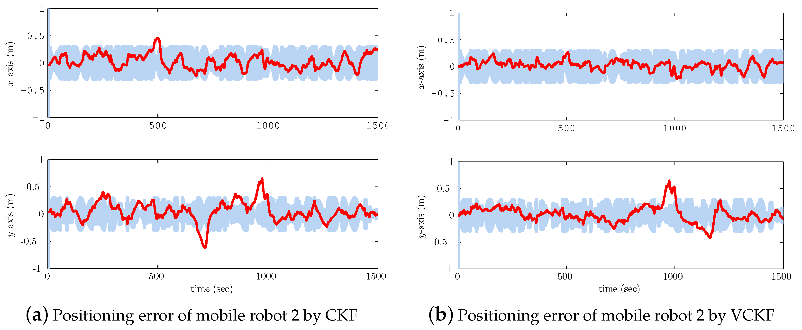
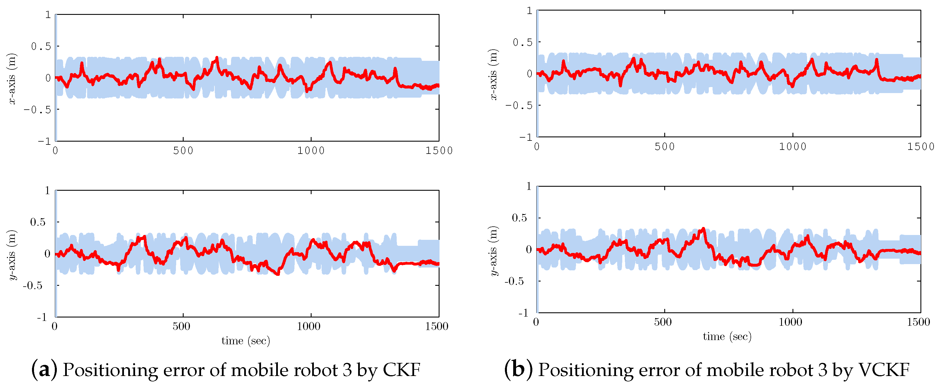
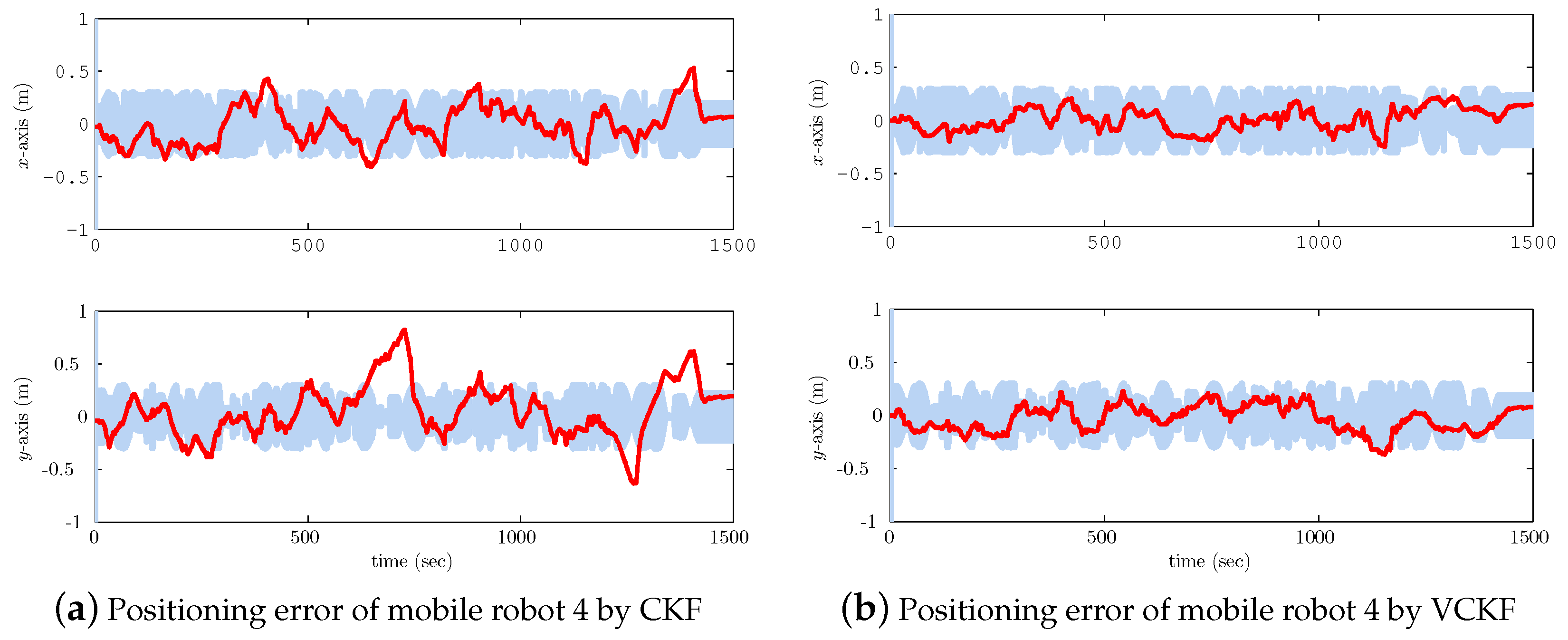
4.2. Cooperative Localization Accuracy Analysis

The normal CKF and the proposed VCKF methods are used to estimate the system state here. State estimation error and associated 3-$\sigma$ error boundaries of each mobile robot are shown in Figure 3, Figure 4, Figure 5, Figure 6 and Figure 7. It can be seen obviously that estimation errors of x- and y-directions with the proposed VCKF algorithm are always sandwiched within associated 3-$\sigma$ error boundaries, while the errors with CKF are out of the associated 3-$\sigma$ error boundaries at some epochs. This implies that, although both the localization scheme based on CKF and the localization scheme based on VCKF are capable of generating a state estimation for each mobile robots, the VCKF algorithm has a better performance.

In order to evaluate the superiority of the proposed cooperative localization algorithm based on VCKF quantitatively, the root mean square (RMS) of each robot’s estimation error has been calculated and summarized in

Table 1. Comparison of the estimation error RMS by CKF and VCKF methods.

Method	CKF		VCKF
	x-Direction	y-Direction	x-Direction	y-Direction
Mobile robot 1	0.156	0.227	0.122	0.136
Mobile robot 2	0.132	0.182	0.087	0.154
Mobile robot 3	0.095	0.134	0.076	0.112
Mobile robot 4	0.201	0.177	0.105	0.126
Mobile robot 5	0.192	0.268	0.108	0.137

. From Table 1, it can be seen that the Root Mean Square (RMS) of x- and y-directions by utilizing the cooperative localization algorithm based on VCKF are smaller than the ones by using algorithms based on CKF. Therefore, this offers further proof that the proposed localization algorithm based on VCKF has better performance in localization accuracy than the algorithm based on normal CKF methods.

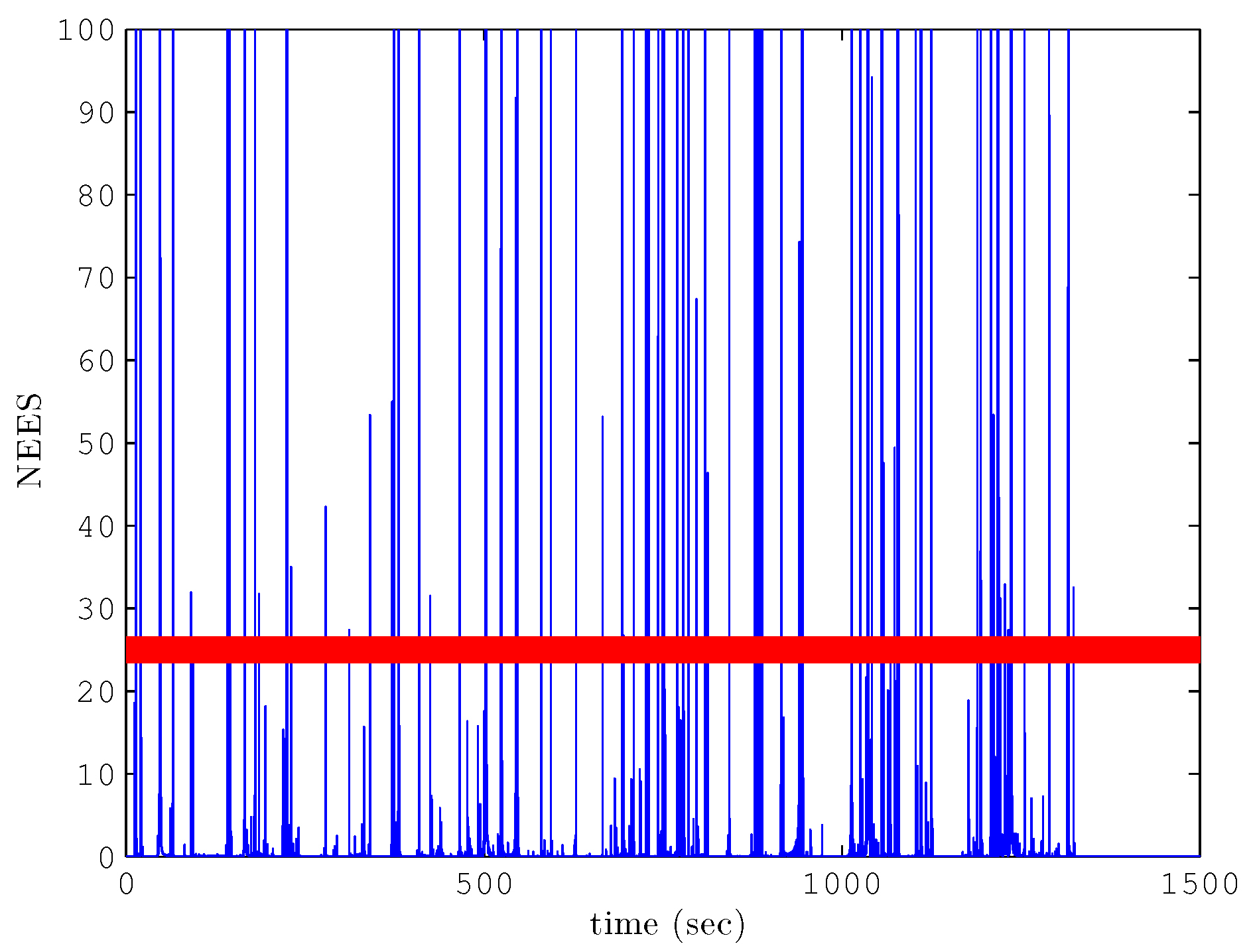
4.3. Algorithm Consistency Analysis

To examine the consistency of the proposed cooperative localization algorithm, Normalized Estimation Error Squared (NEES) is calculated by utilizing

$${ϵ}_{c_i,k}={\mathit{\xi }}_{c_i,k}^{\top }{\mathit{P}}_{c_i,k}^{-1}{\mathit{\xi }}_{c_i,k},$$

(48)

where $ϵ$ is the computed NEES; $\mathit{\xi }$ denotes the pose estimation error at time step k and $\mathit{P}$ represents the estimated error covariance matrix. For a single run, the estimation is consistent if the computed NEES can make the following inequality hold:

$${ϵ}_{c_i,k}\le {\chi }_{n_{\mathit{x}},\delta }^2,$$

(49)

where ${\chi }_{n_{\mathit{x}},\delta }^2$ represents the chi-square distribution with $n_{\mathit{x}}$ Degree of Freedom (DOF) and $\delta$ is the significance level [31]. Therefore, the upper-bound of the $95\%$ acceptance region for the 15-DOF stochastic process is given by ${\chi }_{15,0.95}^2$ and is equal to 24.95.

Figure 8 and Figure 9 give the situations in which the NEES values fall outside of the $95\%$ acceptance region of the cooperative localization algorithm based on CKF and proposed VCKF methods, respectively. In addition, the percentage of the NEES values falling outside the $95\%$ acceptance region based on the CKF method is $8.24\%$, while the one based on VCKF method is $3.78\%$. Thus, it can be seen that the percentages are both less than $10\%$, which is acceptable. Furthermore, we also can see that the cooperative localization algorithm based on VCKF has better performance in consistency than the algorithm based on CKF.

5. Conclusions

In order to overcome the influence on cooperative localization accuracy caused by the uncertainty of measurement noise and the nonlinearity for the MMR system at the same time, the adaptive VCE method was introduced to cubature Kalman filter, proposing a novel cooperative localization algorithm based on the adaptive VCKF method in this manuscript. By using the adaptive VCE method, the statistical property of the system’s noise can be estimated well, and this proposed algorithm can also be applied in nonlinear MMR systems owing to the nonlinear CKF method. Therefore, this proposed algorithm can not only avoid the influence on state estimation caused by the uncertainty of measurement noise availably, but also improve the cooperative localization accuracy for MMR systems significantly. Real experiment data was also used to verify the effectiveness and superiority of the novel cooperative localization algorithm. Furthermore, the experiment results showed that the cooperative localization algorithm based on VCKF has better performance than the one based on CKF both in accuracy and in consistency.

References

1. Sharma, R.; Quebe, S.; Beard, R.W.; Taylor, C.N. Bearing-only Cooperative Localization. J. Intell. Robot. Syst. 2013, 72, 429–440. [Google Scholar] [CrossRef]
2. Wanasinghe, T.R.; Mann, G.K.I.; Gosine, R.G. Distributed Leader-Assistive Localization Method for a Heterogeneous Multirobotic System. IEEE Trans. Autom. Sci. Eng. 2015, 12, 795–809. [Google Scholar] [CrossRef]
3. Wanasinghe, T.R.; Mann, G.K.I.; Gosine, R.G. Decentralized Cooperative Localization Approach for Autonomous Multirobot Systems. J. Robot. 2016, 2016, 2560573. [Google Scholar] [CrossRef]
4. Leung, K.Y.K.; Barfoot, T.D.; Liu, H.H.T. Decentralized Localization of Sparsely-Communicating Robot Networks: A Centralized-Equivalent Approach. Robot. IEEE Trans. 2010, 26, 62–77. [Google Scholar] [CrossRef]
5. Fox, D.; Burgard, W.; Kruppa, H.; Thrun, S. A Probabilistic Approach to Collaborative Multi-Robot Localization. Auton. Robot. 2000, 8, 325–344. [Google Scholar] [CrossRef]
6. Leonard, J.J.; Teller, S. Robust Range-Only Beacon Localization. Ocean. Eng. IEEE J. 2006, 31, 949–958. [Google Scholar]
7. Wanasinghe, T.R.; Mann, G.K.I.; Gosine, R.G. Relative Localization Approach for Combined Aerial and Ground Robotic System. J. Intell. Robot. Syst. 2015, 77, 113–133. [Google Scholar] [CrossRef]
8. Michael, N.; Shen, S.; Mohta, K.; Kumar, V.; Nagatani, K.; Okada, Y.; Kiribayashi, S.; Otake, K.; Yoshida, K.; Ohno, K. Collaborative Mapping of an Earthquake Damaged Building via Ground and Aerial Robots. J. Field Robot. 2014, 29, 832–841. [Google Scholar] [CrossRef]
9. Roumeliotis, S.I.; Bekey, G.A. Distributed Multirobot Localization. IEEE Trans. Robot. Autom. 2002, 18, 781–795. [Google Scholar] [CrossRef]
10. Howard, A.; Parker, L.E.; Sukhatme, G.S. Experiments with a Large Heterogeneous Mobile Robot Team: Exploration, Mapping, Deployment and Detection. Int. J. Robot. Res. 2006, 25, 431–447. [Google Scholar] [CrossRef]
11. Li, H.; Nashashibi, F.; Yang, M. Split Covariance Intersection Filter: Theory and Its Application to Vehicle Localization. IEEE Trans. Intell. Transp. Syst. 2013, 14, 1860–1871. [Google Scholar] [CrossRef]
12. Wang, Y.; Duan, X.; Tian, D.; Chen, M.; Zhang, X. A DSRC-based Vehicular Positioning Enhancement Using a Distributed Multiple-Model Kalman Filter. IEEE Access 2016, 4, 8338–8350. [Google Scholar] [CrossRef]
13. Müller, F.D.P. Survey on Ranging Sensors and Cooperative Techniques for Relative Positioning of Vehicles. Sensors 2017, 17, 271. [Google Scholar] [CrossRef] [PubMed]
14. Masehian, E.; Jannati, M.; Hekmatfar, T. Cooperative mapping of unknown environments by multiple heterogeneous mobile robots with limited sensing. Robot. Auton. Syst. 2016, 87, 188–218. [Google Scholar] [CrossRef]
15. Howard, A.; Matark, M.J.; Sukhatme, G.S. Localization for Mobile Robot Teams using Maximum Likelihood Estimation. In Proceedings of the IEEE/RSJ International Conference on Intelligent Robots and Systems, Lausanne, Switzerland, 30 September–4 October 2002; Volume 1, pp. 434–439. [Google Scholar]
16. Wu, N.; Li, B.; Wang, H.; Xing, C.; Kuang, J. Distributed Cooperative Localization based on Gaussian Message Passing on Factor Graph in Wireless Networks. Sci. China Inf. Sci. 2015, 58, 1–15. [Google Scholar] [CrossRef]
17. Chiang, S.Y.; Wei, C.A.; Chen, C.Y. Real-Time Self-Localization of a Mobile Robot by Vision and Motion System. Int. J. Fuzzy Syst. 2016, 18, 1–9. [Google Scholar] [CrossRef]
18. Zhao, S.; Huang, B.; Liu, F. Localization of Indoor Mobile Robot Using Minimum Variance Unbiased FIR Filter. IEEE Trans. Autom. Sci. Eng. 2016, 99, 1–10. [Google Scholar] [CrossRef]
19. Shan, J.; Wang, X. Experimental Study on Mobile Robot Navigation using Stereo Vision. In Proceedings of the 2013 IEEE International Conference on Robotics and Biomimetics (ROBIO), Shenzhen, China, 12–14 December 2013; pp. 1958–1965. [Google Scholar]
20. Hu, C.; Chen, W.; Chen, Y.; Liu, D. Adaptive Kalman Filtering for Vehicle Navigation. J. Glob. Position. Syst. 2003, 2, 42–47. [Google Scholar] [CrossRef]
21. Aghili, F.; Salerno, A. Driftless 3-D Attitude Determination and Positioning of Mobile Robots By Integration of IMU With Two RTK GPSs. IEEE/ASME Trans. Mechatron. 2013, 18, 21–31. [Google Scholar] [CrossRef]
22. Yu, F.; Sun, Q.; Lv, C.; Ben, Y.; Fu, Y. A SLAM Algorithm Based on Adaptive Cubature Kalman Filter. Math. Probl. Eng. 2014, 2014, 1–11. [Google Scholar] [CrossRef]
23. Sun, J.; Xu, X.; Liu, Y.; Zhang, T.; Li, Y. FOG Random Drift Signal Denoising Based on the Improved AR Model and Modified Sage-Husa Adaptive Kalman Filter. Sensors 2016, 16, 1073. [Google Scholar] [CrossRef] [PubMed]
24. Chang, G.; Liu, M. An Adaptive Fading Kalman Filter based on Mahalanobis Distance. Proc. Inst. Mech. Eng. Part G J. Aerosp. Eng. 2015, 229, 1114–1123. [Google Scholar] [CrossRef]
25. Arasaratnam, I.; Haykin, S. Cubature Kalman Filters. IEEE Trans. Autom. Control 2009, 54, 1254–1269. [Google Scholar] [CrossRef]
26. Arasaratnam, I.; Haykin, S.; Hurd, T.R. Cubature Kalman Filtering for Continuous-Discrete Systems: Theory and Simulations. IEEE Trans. Signal Process. 2010, 58, 4977–4993. [Google Scholar] [CrossRef]
27. Wang, J.G. Reliability Analysis in Kalman Filtering. J. Glob. Position. Syst. 2009, 8, 101–111. [Google Scholar] [CrossRef]
28. Moghtased-Azar, K.; Tehranchi, R.; Amiri-Simkooei, A.R. An Alternative Method for Non-Negative Estimation of Variance Components. J. Geod. 2014, 88, 427–439. [Google Scholar] [CrossRef]
29. Wang, J.G.; Gopaul, N.; Scherzinger, B. Simplified Algorithms of Variance Component Estimation for Static and Kinematic GPS Single Point Positioning. J. Glob. Position. Syst. 2009, 8, 43–52. [Google Scholar] [CrossRef]
30. Leung, K.Y.; Halpern, Y.; Barfoot, T.D.; Liu, H.H. The UTIAS Multi-Robot Cooperative Localization and Mapping Dataset. Int. J. Robot. Res. 2011, 30, 969–974. [Google Scholar] [CrossRef]
31. Bahr, A.; Walter, M.R.; Leonard, J.J. Consistent Cooperative Localization. In Proceedings of the IEEE International Conference on Robotics and Automation, Kobe, Japan, 12–17 May 2009; pp. 3415–3422. [Google Scholar]
Figure 1. Experiment environment and the mobile robots fleet of the University of Toronto, the Institute of Aerospace Studies.
Symmetry 09 00094 g001
Figure 2. Top-view of mobile robots fleet to illustrate the relative measurements between different mobile robots and landmarks.
Symmetry 09 00094 g002
Figure 3. (a) Positioning estimation error curves of mobile robot 1 by utilizing Cubature Kalman Filter (CKF); (b) Positioning estimation error curves of mobile robot 1 by utilizing improved algorithm based on CKF and VCE methods, denoted by VCKF. The red solid line indicates the estimation error while the shaded regions indicate double-sided 3- σ error boundaries.
Symmetry 09 00094 g003
Figure 4. (a) Positioning estimation error curves of mobile robot 2 by utilizing CKF; (b) Positioning estimation error curves of mobile robot 2 by utilizing VCKF. The red solid line indicates the estimation error while the shaded regions indicate double-sided 3- σ error boundaries.
Symmetry 09 00094 g004
Figure 5. (a) Positioning estimation error curves of mobile robot 3 by utilizing CKF; (b) Positioning estimation error curves of mobile robot 3 by utilizing VCKF. The red solid line indicates the estimation error while the shaded regions indicate double-sided 3- σ error boundaries.
Symmetry 09 00094 g005
Figure 6. (a) Positioning estimation error curves of mobile robot 4 by utilizing CKF; (b) Positioning estimation error curves of mobile robot 4 by utilizing and VCKF. The red solid line indicates the estimation error while the shaded regions indicate double-sided 3- σ error boundaries.
Symmetry 09 00094 g006
Figure 7. (a) Positioning estimation error curves of mobile robot 5 by utilizing CKF; (b) Positioning estimation error curves of mobile robot 5 by utilizing and VCKF. The red solid line indicates the estimation error while the shaded regions indicate double-sided 3- σ error boundaries.
Symmetry 09 00094 g007
Figure 8. The Normalized Estimation Error Squared (NEES) of the cooperative localization algorithm based on VCKF. The red straight line indicates χ 15 , 0 . 95 2 and the blue solid line indicates ϵ k ; 3.78 percent of ϵ k are above the red straight line.
Symmetry 09 00094 g008
Figure 9. NEES of the cooperative localization algorithm based on CKF. The red straight line indicates χ 15 , 0 . 95 2 and the blue solid line indicates ϵ k ; 8.24 percent of ϵ k are above the red straight line.
Symmetry 09 00094 g009