Article

Hierarchical Meta-Learning in Time Series Forecasting for Improved Interference-Less Machine Learning

1
Department of Computer Science and Software Engineering Xi’an Jiaotong-Liverpool University, Suzhou 215123, China
2
Department of Computer Science, University of Liverpool, Liverpool L69 3BX, UK
*
Author to whom correspondence should be addressed.
Symmetry 2017, 9(11), 283; https://doi.org/10.3390/sym9110283
Submission received: 24 October 2017 / Revised: 1 November 2017 / Accepted: 1 November 2017 / Published: 18 November 2017
(This article belongs to the Special Issue Novel Machine Learning Approaches for Intelligent Big Data)

Abstract

:
The importance of an interference-less machine learning scheme in time series prediction is crucial, as an oversight can have a negative cumulative effect, especially when predicting many steps ahead of the currently available data. The on-going research on noise elimination in time series forecasting has led to a successful approach of decomposing the data sequence into component trends to identify noise-inducing information. The empirical mode decomposition method separates the time series/signal into a set of intrinsic mode functions ranging from high to low frequencies, which can be summed up to reconstruct the original data. The usual assumption that random noises are only contained in the high-frequency component has been shown not to be the case, as observed in our previous findings. The results from that experiment reveal that noise can be present in a low frequency component, and this motivates the newly-proposed algorithm. Additionally, to prevent the erosion of periodic trends and patterns within the series, we perform the learning of local and global trends separately in a hierarchical manner which succeeds in detecting and eliminating short/long term noise. The algorithm is tested on four datasets from financial market data and physical science data. The simulation results are compared with the conventional and state-of-the-art approaches for time series machine learning, such as the non-linear autoregressive neural network and the long short-term memory recurrent neural network, respectively. Statistically significant performance gains are recorded when the meta-learning algorithm for noise reduction is used in combination with these artificial neural networks. For time series data which cannot be decomposed into meaningful trends, applying the moving average method to create meta-information for guiding the learning process is still better than the traditional approach. Therefore, this new approach is applicable to the forecasting of time series with a low signal to noise ratio, with a potential to scale adequately in a multi-cluster system due to the parallelized nature of the algorithm.

1. Introduction

In forecasting time series data, machine learning has been commonly applied in a number of real world scenarios such as stock market prediction, weather/natural phenomena prediction, energy management, human activity classification, control engineering and sign language identification. In such predictions, the accuracy performance correlates to the quality of the data being modelled; in essence, the usefulness of the prediction heavily depends on the training sample and its clarity. The primary aim of this research is to develop a systematic technique to enhance the machine learning process by eliminating noise which is observable in short and long term trends of the time series.
Other research in the area of time series forecasting have applied a number of techniques including the hidden Markov model [1], support vector regression (SVR) [2], fuzzy logic [3], dynamic time warping [4], and more commonly the artificial neural network (ANN). These techniques are able to closely model the training data, but, due to noise within such data, a high error rate can be observed in the test data.
As an extension to previous work [5] in time series forecasting, in which we have proposed the guiding of the model-building stage, some important improvements to the algorithm have led to increased performance in both training and test accuracies. To accurately learn short-term and long-term trends within the data in the presence of noise or conflicting information, meta-information generated from patterns seen in the training data are learned simultaneously from predetermined segments of the time series during the training stage.
We therefore developed an algorithm to exploit component trend patterns with a high information-bearing capacity and eliminate other low information-bearing components to prevent the model from learning inconsistent trends. As noted in [5], other researchers have proposed other solutions in attempt to reduce the impact of noise. These include the autoregressive integrated moving average-noise (ARIMAN) model [6], and the forward search method [7] which works by smoothening the data and is useful only in time series with repeating patterns.
The research study covered in this paper details the extension of the empirical mode decomposition (EMD) applied to noise reduction in a nonlinear autoregressive exogenous model (NARX) neural network during machine learning [5], and further comparison is carried out with long short-term memory (LSTM) [8]. In the next section, some background on the hypotheses and fundamental algorithms that were used will be described. The method section covers dataset pre-processing, the proposed algorithms, and the learning process. Then, the results and discussions are then presented and concluded with future research directions.

2. Background

2.1. Motivation for Noise Elimination in Time Series Data

Noise in time series forecasting can have a cumulative impairment on the prediction of values n-steps ahead; therefore, algorithms that are able to build an accurate model based upon an available data sequence n steps before whilst reducing the impact of high or low frequency noises within the data can be useful in predicting short- or long-term values. The impact of noise is noticeable when predicting values many steps ahead; it is therefore important to identify low or high frequency components that are inconsistent. From previous research in [9], the importance of noise management has been stated, and from our work in [5] we observed that noise can occur in both low or high-frequency components of the time series.

2.2. NAR and NARX

In time series prediction, the non-linear autoregressive model (NAR) is commonly used when a sequence of data has only one series, y(t); the future value is predicted using only d number of past values, where the function f can be estimated with a multilayer perceptron (MLP) [10]:
y ( t ) = f ( y ( t 1 ) , ,   y ( t d ) )
On the other hand, when time series forecasting has one or several input series (in a vector x ) which are necessary for prediction thereby utilizing both input vector and outputs of past values over a fixed window, d, a non-linear autoregressive exogenous model (NARX) is required:
y ( t ) = f ( x ( t 1 ) , ,   x ( t d ) ,   y ( t 1 ) , ,   y ( t d ) )
For example, rather than using the past week’s temperature alone to predict tomorrow’s temperature, a more accurate prediction can be achieved if other factors such as wind speed, humidity and seasonal trends among others are applied as inputs and used to train the artificial neural network in conjunction with the temperatures of past days or weeks. Therefore, Figure 1 shows a fundamental NARX model structure with a delayed or lagged feedback from the output connected back to the input unit to create a feedback loop.
The NARX model can also be expressed in a state-space form as discussed in [10], wherein additional properties can be illustrated in the form:
y i ( t + 1 ) = { Ψ [ x ( t ) , y ( t ) ] i = 1 y i 1 ( t ) i = 2 , , d
where y is a scalar output at a given time, the subscript term i controls the limit of recursion within the predefined delay window, function Ψ represents MLP mapping, and d is the order (or output delay window). By deriving the Jacobian of the state-space map of Equation (3), it is revealed that the NARX network will deteriorate due to long-term dependencies and vanishing gradients [10]. It may therefore be intuitive to learn short-term and long-term patterns separately in a hierarchical manner to prevent interference; this is further discussed in our proposed learning algorithm in Section 3.4.

2.3. Moving Average

Moving average [11] is a statistical data analysis technique used to smoothen a sequence of data points. It uses a window or period over which a fixed number of data points are averaged in steps from the initial to the final values. With this method, high-frequency fluctuations are erased depending on the size of the rolling window; therefore, finding the optimal window size is heavily dependent on the use-case. Variations of the moving average commonly used in the technical analysis of data include cumulative moving average, weighted moving average, and the exponential moving average, among others. In this research, we applied the simple moving average, which is an unweighted mean of the data within each window period. It was chosen because the resultant trend has the highest similarity to the original series by calculating the rolling mean over a relatively small window size.
m o v i n g   a v e r a g e ( t ) = i = 0 d 1 y ( t i ) d
where d is the window period, and y(t) the t-th element in the time series. While this method may be able to eliminate short-term noise from the data, it does not take into account the effects of long-term noise and the erosion of important short-term trends on the model.

2.4. Empirical Mode Decomposition

Empirical mode decomposition (EMD) was developed as a fundamental part of the Hilbert–Huang transform to iteratively divide a signal into component signals called intrinsic mode functions (IMF) [12]. A technique such as EMD is capable of producing structural primitives [9] or building-block trends, based on the hypothesis that past patterns are highly likely to repeat. This enables easier detection of new/unseen information-bearing patterns or, on the other hand, noise. It is a robust algorithm with several improvements such as extrema interpolation, stopping criterion, and boundary effect [13] to enable accurate reconstruction of the original signal by summing up each derived IMF.
The procedure of detecting intrinsic oscillation in the signal/time series involves firstly identifying local extrema, after which an iterative sifting process is used to derive each intrinsic mode function. The iterative sifting process stops after one of two stopping rules is satisfied. Either the absolute value of a potential IMF, hi, is less than the tolerance level,
| h i ( t ) | < t o l e r a n c e   l e v e l
or when the variation in a successive IMF candidate is within the tolerance level as expressed in Equation (6) [14].
t ( h i ( t ) h i 1 ( t ) h i 1 ( t ) ) 2 < t o l e r a n c e   l e v e l
The method for extrapolating the end points of the signal has significant importance due to its effect on the accuracy of signal reconstruction [13]. Since we chose to work with the EMD implementation in [13], their solutions to this effect were to consider end points as maxima and minima simultaneously according to the nearest extremum, thereby enforcing all IMFs to be zero at those points and ensuring alternation between maxima and minima.
The complete empirical mode decomposition can be achieved as follow [5]:
STEP 1:
Let hi(t) = y(t), and i = 1.
STEP 2:
Find some local minima and maxima in hi(t).
STEP 3:
Connect all identified maxima and minima by a cubic spline as the upper envelope upi(t) and lower envelope lowi(t), and calculate local mean as mi(t) = [upi(t) + lowi(t)]/2.
STEP 4:
Update as hi(t) = hi(t) − mi(t).
STEP 5:
Ensure hi(t) fulfils the requirement of IMF. If not, then redo STEP 2 to STEP 5. If done, then IMFi(t) = hi(t), i = i + 1 and hi(t) = y(t) − IMFi−1(t).
STEP 6:
Check if hi(t) is a monotonic function or not. If it is not then redo STEP 2 to STEP 5 for the next IMF. If it is monotonic then hi(t) = rc(t) and end the EMD process.
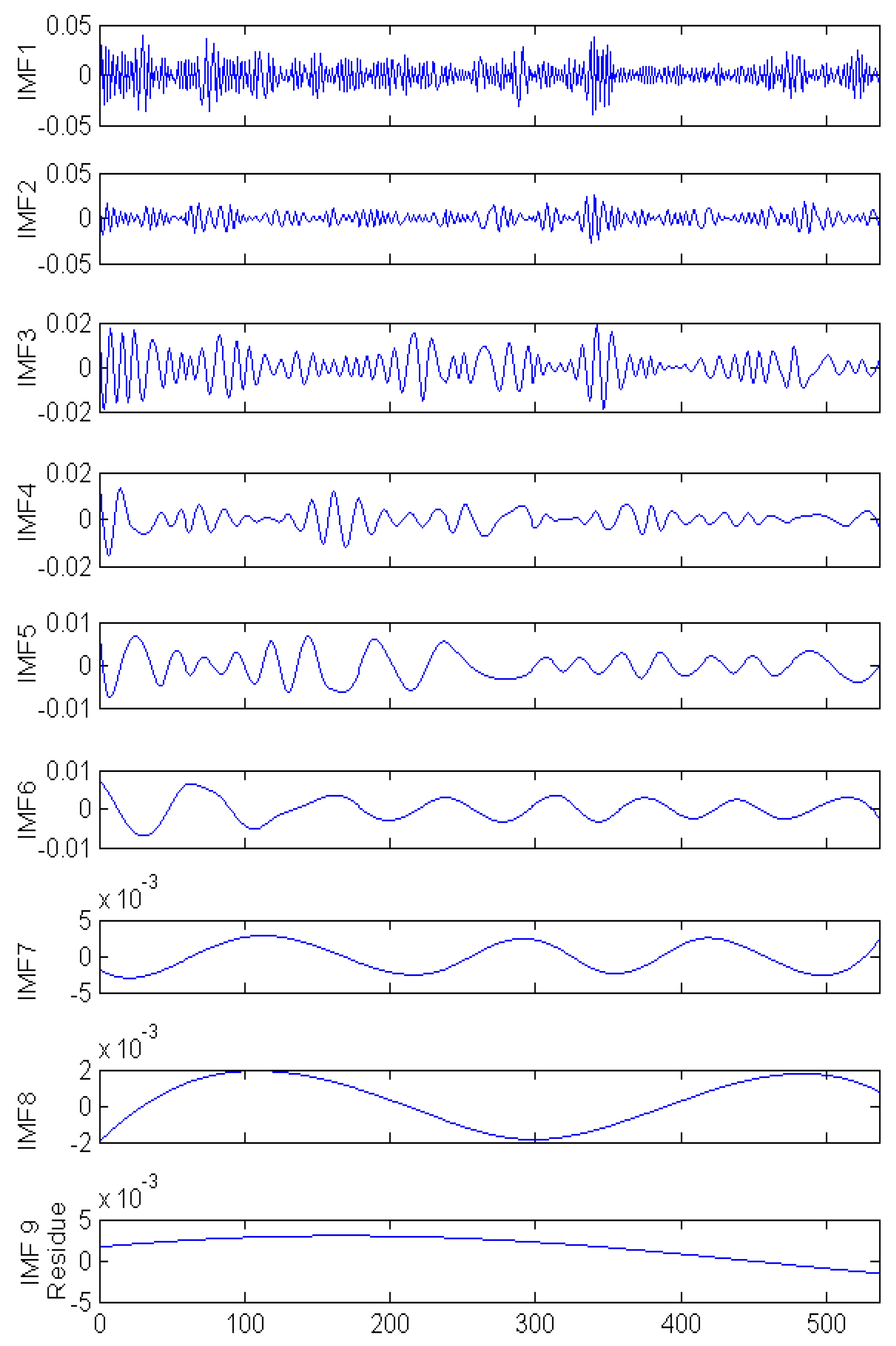
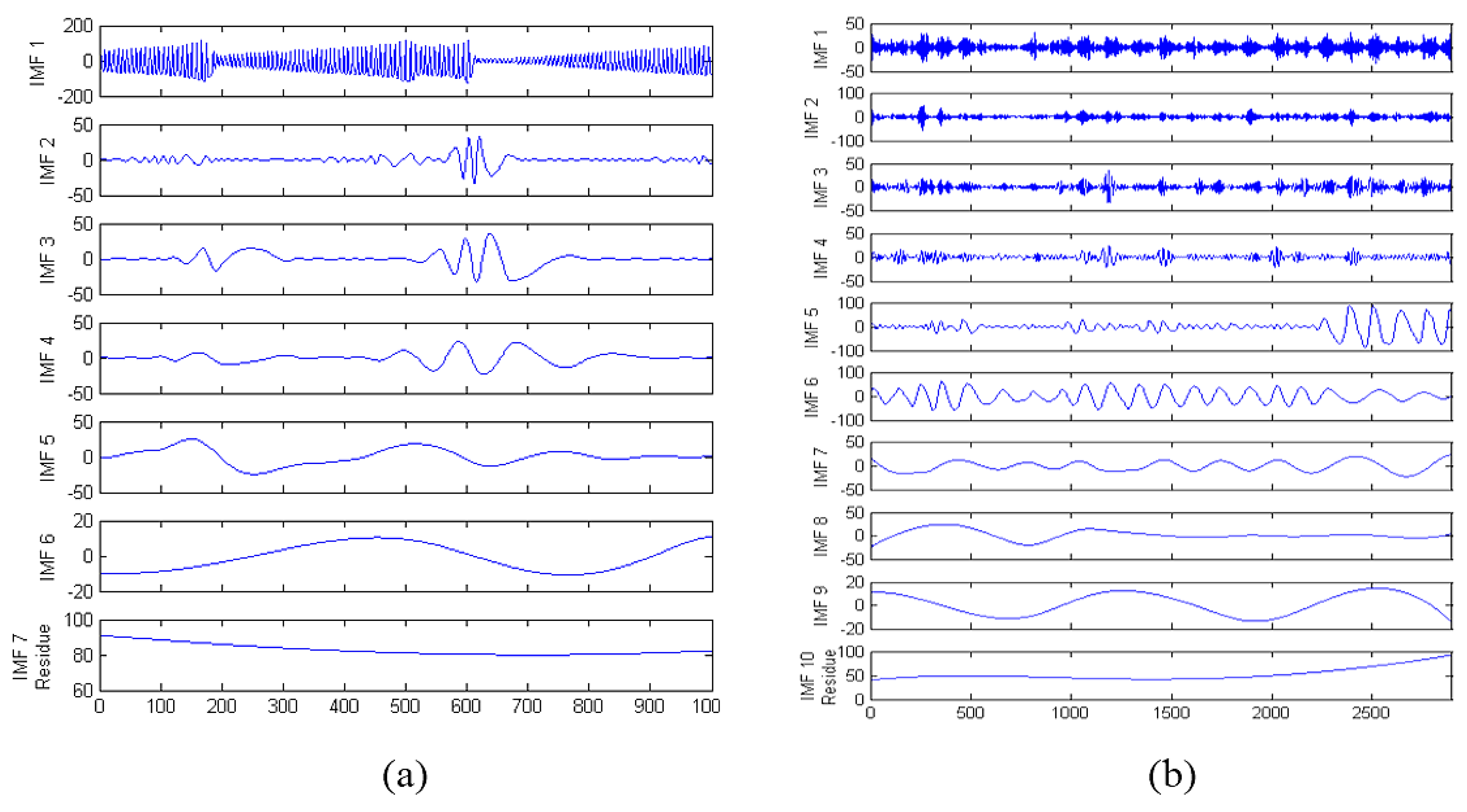
An example of the EMD outcome is shown in Figure 7, and the result consists of c IMF functions and a residue, rc(t), which is expressed in the following equation as:
y ( t ) = i = 1 c I M F i ( t ) + r c ( t )

3. Method

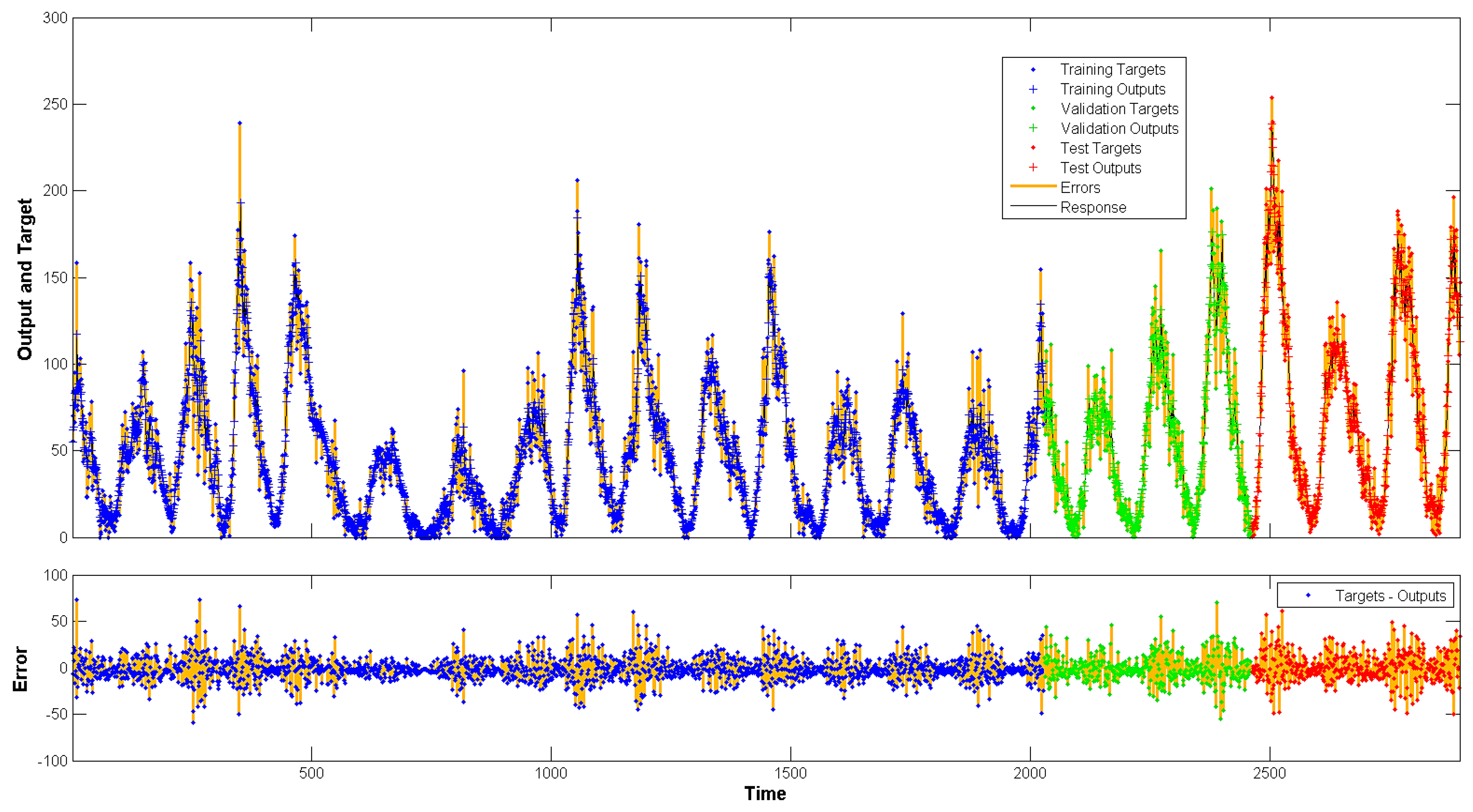
In this study on meta-learning for time series forecasting, we selected four data sets from physical sciences and financial markets. The data was spilt into training, validation, and testing sets sequentially. This means that we partitioned the first 70% of the data sequence for training, and then the next 15% was allocated for validation, while the final 15% was for testing the performance of the derived machine learning algorithm for comparison with the traditional approach. Figure 2 shows an output response plot in which orange vertical lines identify how much deviation (error) the predicted value has from the target value; meaning that time steps with more prominent orange lines have an inaccurate prediction. More importantly, this graph highlights how the data was divided as the blue, green, and red sections denote the training, validation, and test data respectively. A window size (or lag/delay) is required in time series learning, which is the number of data points made available to the model before the actual data point that is being predicted. In the case of this experiment, two window sizes—5 and 10—are explored in order to identify trends within the data. These could aid in detecting weekly or fortnightly patterns, especially in the stock market data. Finally, the traditional non-linear autoregressive neural network (NAR) was used exclusively on the datasets, while the non-linear autoregressive exogenous neural network (NARX) was used for training in combination with each of the learning algorithms described in Section 3.2. The exogenous input to the artificial neural network is important because we use this means to introduce meta-information to guide the learning process as the model is built. Similarly, the long short-term memory (LSTM), which is a variation of the recurrent neural network (RNN) [8], allows additional input, and therefore this algorithm is tested as well.

3.1. Dataset and Sample Selection

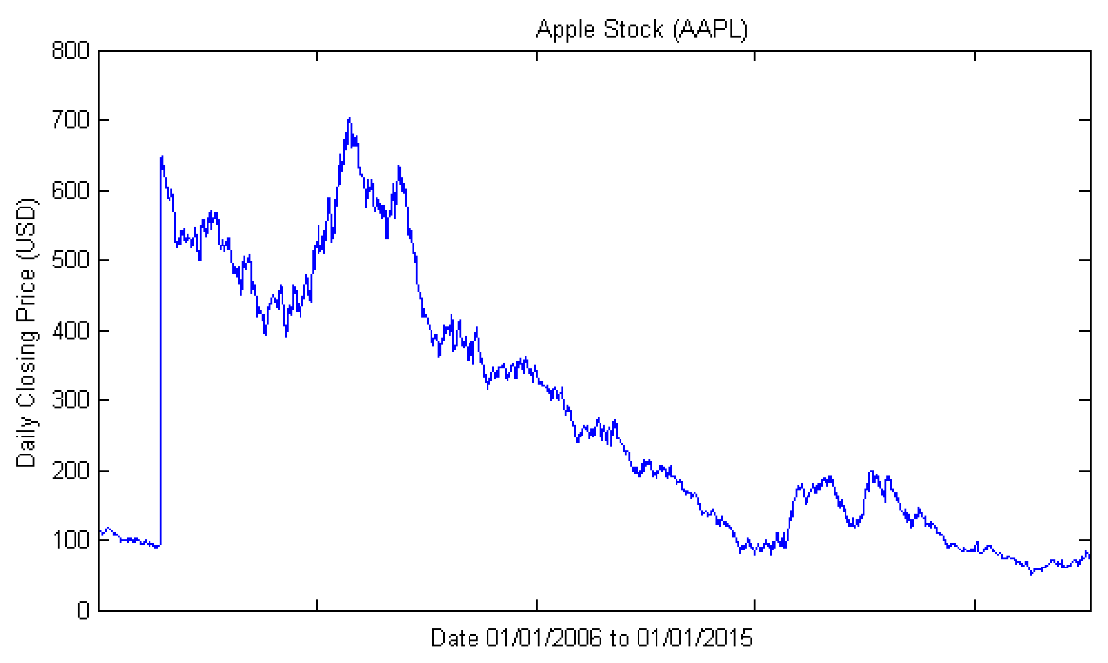
The first-time series dataset is from Apple Inc., a leading manufacturer of mobile communication devices and personal computers. Its stock data was retrieved from Yahoo Finance website in a similar method as [15], in which they collected daily closing prices from 01/01/2006 to 01/01/2015 having minimum and maximum values of 50.67 and 702.1 respectively (see Figure 3). This dataset will be referred to as AAPL in the following sections.
Secondly, the sunspot dataset is derived from a recurrent temporary natural phenomenon that causes visible dark spots on the sun’s surface due to its magnetic activity. Some research has been carried out to identify the trends inherent in these solar cycles [16]. We have selected this long-duration dataset, which contain a monthly record over a period of 240 years from [16]. It has 2899 entries with values ranging between 0 and 254 as shown in Figure 4 and this time series will be referred to as SOL.
The third-time series task involves data that was used at the Santa Fe time series competition and was generated from the transition of far-infrared laser intensity pulsations from periodic to chaotic [17]. The time series (referred to as SFL) is within the range of 2 to 255, and 1000 points with several bell-shaped oscillations, as seen in Figure 5.
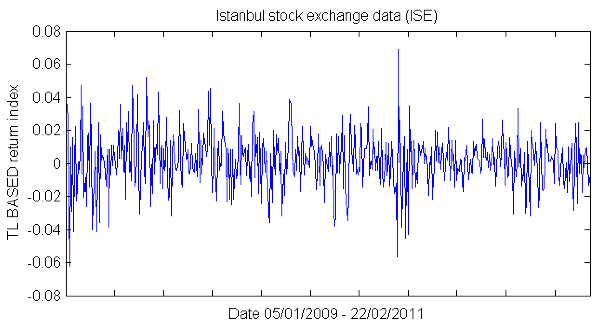
Finally the Istanbul Stock Exchange (referred to as ISE) time series was obtained from [18], where they explored its relationship to other international stock indices using a hybrid radial basis function neural network [18]. In our research, we utilized a single data column from that dataset called “TL based return index”. It contains 536 records over a period from 05/01/2009 to 22/02/2011 with minimum and maximum values of −0.0622 and 0.0690 shown in Figure 6. Figure 7 shows the ISE decomposition result after running the EMD routine and the plots are ordered from highest to lowest frequency.

3.2. Algorithms and Learning process

Three main methods are compared in this survey; they include:
(1)
The traditional approach, in which the time series is directly used by the NAR neural network for training. We denote this as NAR.
(2)
The NARX neural network is presented with the original time series as input, and an additional pre-processed meta-information from the moving average technique. Denoted as NARX-MA.
(3)
Finally, the NARX neural network inputs contain both the meta-information output of the EMD de-noising algorithm (see Section 3.4 for definition) and the original time series. Referred to as NARX-EMDv2 in this paper.
In order to compare our contribution to other algorithms, we ran the experiment on nonlinear autoregressive models with and without the meta-information; additionally, a similar experiment using a long short-term memory (LSTM) was tested and the results are presented in Appendix A. The LSTM is an artificial neural network with a chain-like connection that enables it to loop information between sigmoid function processing units, which are comprised of an input gate, forget gate, and an output gate. These gates control the LSTM’s states to adequately deal with sequential data, thus making it popular in the field of natural language processing (NLP). The RNN and its variants such as LSTM, and gate recurrent unit (GRU) can be characterized as having a sequential architecture [8]. For this reason, we present the complementary results and discussion for the experiment using the original LSTM for forecasting versus our modified LSTM-MA, and LSTM-EMDv2 algorithms.

3.3. NARX-MA Algorithm (Moving Average)

As the name implies, the original time series was pre-processed by a rolling average calculated over two windows sizes—W = {5, 10}—for comparison. Since moving average finds the mean of the past W points, an effect on the output is that the first W-1 points will be null. To ensure that we have a data sequence with equal size as the original series, the average of the first n < W points were imputed as the average of the preceding n available points.

3.4. NARX-EMDv2 Algorithm (EMD de-Noising Version 2)

In our previous research on using meta-learning for interference elimination using EMD, we proposed to identify and eliminate noise within a time series as follows [5]:
STEP 1:
Run the EMD routine on the time series data using normal parameters in [13]. Let N be the total number of IMFs produced and set the number of neural network hidden neuron to 75% of N (rounded up). [The parameters used are: resolution (qResol) = 40 dB, residual energy (qResid) = 40 dB, and gradient step size (qAlfa) = 1. The tolerance level is determined by resolution (qResol) which terminates the IMF computation [13].]
STEP 2:
Based on use-case, set the input and feedback delays [i.e., number of past values presented to the artificial neural network model for prediction].
STEP 3:
Create N combinations of all IMF whilst progressively excluding higher frequency IMF in each combination.
STEP 4:
Create a modified input series x(t) from the remaining IMF in each combination which will either be summed [as a single input] or included directly [as multiple inputs] into the input [of the artificial neural network].
STEP 5:
Train the NARX model with each combination and test the performance to reveal a combination that contributes to noise reduction.
STEP 6:
If noise reduction requirement is not met, decrease N and repeat from STEP 3.
Even though the algorithm in [5] outperformed the standard approach to learning time series tasks in training time and prediction accuracy, we highlighted some drawbacks and sought to improve the algorithm here with EMDdenoiseV2.
Firstly, it was earlier assumed that noise will mostly be within high frequency component IMF, but we discovered in [5], after progressively excluding some low frequency IMF, that the mean square error (MSE) dropped. Therefore, instead of sequentially removing IMF components from high to low frequency, we followed a hierarchical structure to train several sub-NARX ANN on the first level with only one IMF excluded at a time for training and re-evaluation, and then eliminated the IMF with the least MSE reduction.
Secondly, as interference may not be persistent throughout the entire data series, we divided each part of the training set into sequential batches before identifying the noisy components. The number of divisions (10 and 50, as noted in Table 1, Table 2, Table 3 and Table 4) were heuristically selected, keeping in mind that a high number of divisions in a small data series will make each partition too small to identify trends (or noise) and can significantly increase the computational requirement needed to accurately learn each partition.
Algorithm 1: EMDdenoiseV2
Input: Time Series Data, x; Heuristic Data Division Value, d.
Output: Denoised meta_info;
1 sequentially divide x into d approximately equal partitions
2 for each partition p to dth
3 | run EMD routine
4 | initialize sub-NARX ANN and train by exempting one IMF at a time
5 | identify IMF elimination that contributes to lowest MSE
6 | sum valid IMF to create meta_info for pth partition
7 end
8 append meta_info from each partition sequentially to form series length equal to x.
9 return meta_info
In order for the algorithm (Algorithm 1) to accommodate a hierarchical structure for trend discovery, as shown in Figure 8, the training series is first divided into partitions which are further decomposed by EMD. Machine learning on the first layer of the hierarchy is carried out in parallel by each sub-NARX ANN (for each partition’s set of IMFs) to discern which component IMF to use in meta_info building. After the sub-level training and generation of meta-information is completed, a NARX ANN on the next hierarchy level is initialized for training with the original time series along with the meta_info (de-noising knowledge) output from EMDdenoiseV2 algorithm. The meta_info is utilized as an exogenous input for the performance boost we present in the results and discussions sections. For the sub-NARX ANN training, we set the number of hidden neurons to 75% of number of IMF generated. For comparison, we used a lag of 5 and 10 for the number of past values presented to the NAR, NARX, and LSTM models for prediction in this survey.
In the flowchart above, the complete process of creating and utilizing the new knowledge discovered from the EMDdenoiseV2 algorithm in a hierarchical structured approach is illustrated. After the noise inducing decompositions in each division have been identified and rejected by the first layer of NARX learners for local trends, a secondary layer of NARX, which learns the global trend, is then used to produce the final prediction based on both the meta-information output of the previous layer and also the original time series.

4. Results

The experiments were performed on an Intel® Xeon® E5-1660 hexa-core CPU at 3.3 GHz with 8 GB of RAM, and the MATLAB [19] environment and the Keras Python API [20] were used for implementation and simulation. The average simulation time over 100 repetitions was recorded, including the average training error, average test error, lowest (i.e., best) test error, and p-value of each algorithm’s test errors versus that of the algorithm with the lowest observed average test error. The maximum training epoch was fixed at 250. In order to prevent overfitting and improve generalisation, the early stopping technique was applied to terminate training and revert the artificial neural network to the state with minimum error if the validation error increases consecutively for 10 iterations.
The performance function used in the experiment is the mean square error and the results here are expressed as the normalized mean square error (NMSE), which produces a non-negative mean from the summation of squared errors, where σ2 is the variance of a series of length n, yi is the target, and ŷi is the predicted value expressed in Equation (8). It represents the absolute deviation of the prediction from the target; therefore, a perfect model will have an NMSE of 0.
N M S E = 1 σ 2 n i = 1 n ( y ^ i y i ) 2
The Student’s t-test is also used to highlight the statistical significance of the algorithm over the conventional approach by observing the p-value. A p-value of 0.05 indicates a significant improvement with only 5% similarity and thus any p-value less than this threshold supports the rejection of the null hypothesis, therefore accepting that the compared hypothesis or algorithm is superior.
Each separate row labelled in Table 1, Table 2, Table 3 and Table 4 below has been colour coded with a gradient from red through yellow to green, where deep red cells show poor performance (with high NMSE), and bold values with deep green denote best performance (with low NMSE). To explore the effect of making a prediction several steps ahead, rather than a potentially trivial one-step-ahead prediction in many related research, we employed the data partitioning scheme mentioned in the method section to create the training, validation, and test series.

5. Discussions

In comparing NAR, NARX-MA, and NARX-EMDv2, we included the normalized mean square error results when the division was set to 10 and 50 to explore the effect on the prediction accuracy of the proposed algorithms. The division value controls the number of partitions on which the first layer of noise elimination is executed upon, therefore we explore the range of values to identify the effect of performing excessive noise reduction as the value increases. Similarly, the experiment was conducted with an LSTM neural network.

5.1. Performance on Non-Linear Autoregressive Neural Networks

The result from Table 1 on AAPL reveals that NARX-EMDv2 has a lower NMSE in comparison to the conventional NAR method and the NARX-MA, both in training accuracy and testing accuracy for delay windows of 5 and 10. The reduction of error in both training and testing scenarios indicates a good generalization of the model. Overall, when the NARX-EMDv2 is given a wider delay window, some performance increase is noted, even though a similar observation can be seen for the other two methods. Additional numbers of neurons did not show a consistent performance boost. On the other hand, the NAR and NARX-MA models were considerably influenced by noise, as the training errors are higher, and overfitting is observed with more neurons. NARX-MA test performance is the worst of the three on AAPL. Finally, the training time does not reveal any correlation with accuracy except that networks with a higher number of hidden neurons spent more time on training.
SOL time series shows that excessive noise reduction has an adverse effect on the performance when many batches are created with each containing only a small series of data. Overfitting on the training data is consistently noticed in NAR, NARX-MA, and NARX-EMDv2 with 50 hidden neurons. We observe similar results as in AAPL when NAR underperforms, and NARX-EMDv2 confirms the noise detection and elimination hypothesis supersedes NAR-MA by decomposing the time series to find and remove component trends that do not contain information necessary for accurate prediction. There is no significant difference when the model is built upon a delay window of 5 or 10.
The NARX-EMDv2 is unable to learn the SFL time series with better accuracy than the other two methods. Even with window lag of 5 and 10, the training NMSE is significantly higher when compared to NAR and NARX-MA. On this time series task, all three algorithms performed better with a longer delay window of 10 steps and more artificial neural processing units. To understand the reason for NARX-EMDv2’s performance on the SFL time series data, the empirical mode decomposition is plotted and compared with that of SOL in Figure 9. As shown in Figure 9a, the SFL generated wave is complex and the decomposition yields no intrinsic pattern as compared to SOL and ISE. The SOL and ISE graphs in Figure 7 and Figure 9b show periodically repeating trends which are necessary for the learner to build an accurate model. Note that the first IMF in Figure 9a is observed to have high similarity with the original time series in Figure 5, which means the decomposition process was comparatively unsuccessful. This reconfirms that the hypothesis for interference removal necessitates an accurate decomposition of the data.
The periodically repeating trends visible in ISE time series IMF decomposition shown in Figure 7 are information-bearing, and this explains the substantial gain in accuracy using NARX-EMDv2. The best result is obtained with a window size of 10 (a fortnight in trading days) rather than a weekly base (window size 5). Furthermore, the time required to train the NARX-EMDv2 learner was relatively similar to the traditional NAR method.

5.2. Performance on Long Short-Term Memory Neural Network

Utilizing the LSTM recurrent neural network for hierarchical meta-learning also reveals some significant enhancement on the model’s accuracy (see Appendix A).
In the AAPL time series task, the LSTM-MA algorithm’s performance accuracy and standard deviation is statistically better than those of LSTM and LSTM-EMDv2 methods; additionally, the feedback lag of 10 step resulted in a lower NMSE across all algorithms, while overfitting is prominent with lag 5. The best performing NARX-EMDv2 algorithm (i.e., lag: 5) with a lower NMSE required approximately half the time of LSTM-MA.
The seasonality of the SOL data series can be noticed visually in Figure 4. The EMDdenoiseV2 algorithm exploits such seasonality, which produced a lower test error in both NARX and LSTM time series models. There was no significant impact of lag in both of the NARX-EMDv2 results, but LSTM-EMDv2 with lag of 10 significantly outperformed the model with a shorter lag.
The SFL experiment reveals a unique case in which a relatively unsuccessful decomposition offers no enhancement to meta-learning. In this case, addition of extra hidden units to the original LSTM network was adequate to obtain the lowest NMSE at the expense of longer training time.
On ISE, the performance of NAR and LSTM models are similar, but the LSTM required about ten times more training duration on average. Even though the EMDdenoiseV2 meta-learning modification enhanced the results in both NARX and LSTM algorithms, the NARX-EMDv2’s normalized mean square error is considerably lower than its LSTM-EMDv2 counterpart.
In general, a comparison with the results from the alternative implementation using an LSTM, we see that the NARX implementation is significantly faster and produces a lower average NMSE.

5.3. Potential Application

Based on the positive experimental results in both NARX and LSTM, this proposed method of error elimination on subsections of the time series using learners in multiple levels (two in this survey) affirms the benefit of a hierarchical network and the importance of structural-based learning, whereby interference reduction is performed on smaller divisions of the series before recombination with subsequent sections for further noise detection as you traverse up the hierarchy. Achieving a structured decomposition aims to discover a hierarchy of concepts which can assist in making a connection between input trends, intermediate patterns, and target models/concepts [21].
The motivation for this proposed algorithm is to address the challenge of forecasting trends with noise and conflicting information. Thus, it can be applied to systems in which a low signal to noise ratio is frequently observed. Compared to feature selection in a high dimensional classification task, the EMDdenoiseV2 algorithm tackles this issues by sorting the decomposed trends from highest to lowest contribution and then eliminating the trends that induces entropy.
Additionally, the EMD algorithm, which is utilized for the time-domain decomposition of the data, has been shown to be a computationally efficient method with a proven time complexity of O(nlogn), where n is the length of the time series data [22]. Therefore, the forecast accuracy gained by meta-learning is not achieved at a significant time/computational cost; moreover, steps in the EMDdenoiseV2 hierarchical meta-learning algorithm are designed for parallelization. Based on the efficient and parallelized nature of the algorithm, it can potentially fit and scale well in a multi-cluster system, thereby it is more suitable than traditional time series methods for big data analytics.
Therefore, the advantages include easy extension/enhancement of other time series algorithms and the capacity to make accurate prediction many steps ahead. A limitation can be noted with time series data which do not produce recognisable component patterns after empirical mode decomposition.

6. Conclusions

In previous research on interference reduction in classification tasks, incremental attribute learning (IAL) was used to identify noises within the training data by learning on a grouping of attributes which were mutually beneficial and contributed to training accuracy while separately training different sub-networks for interfering attributes [23]. In the case of time series tasks where only a sequence of past output data is available, a different approach to interference elimination has thus been proposed here. By decomposing fixed periods within the time series using EMD, we are able to identify noisy components before summing the remaining beneficial IMFs for each period and finally re-joining the meta-information sequentially for the higher hierarchy artificial neural network training, as we have demonstrated with NARX and LSTM.
With the results seen in the benchmark datasets surveyed in these experiments, we have shown the benefits of the new approach over the conventional NAR and LSTM methods in cases where the time series can be properly decomposed into meaningful trends using empirical mode decomposition.
The significant contribution of this algorithm is its resilience to noise that may have occurred within a short period or over a long period in the series. Utilizing a hierarchically structured order for training sub-networks on small divisions (local learners) before another learner is trained with the complete series (global learner) provides the machine learner with a better view of the data. This is an advantage when selection of an optimal window size is non-trivial.
Finally, the pre-processing time and training time for the first level sub-networks did not increase the total training time significantly because each division can be trained concurrently.
Further research directions to be explored include automatic detection of patterns present in IMFs, and using such information for the selection of the best meta-learning algorithm and its parameters for a hierarchical structure. Examples of such parameters include the number of layers/levels necessary to produce best prediction performance.
Additionally, a recursive divide and conquer approach to the input time series division, in step 1 of the EMDdenoiseV2 algorithm, can create a larger applicability and reduced computational complexity of the algorithm, since noise may not be present in all divisions.

Acknowledgments

This research is supported by China Jiangsu Provincial Science and Technology programme under Grant No. BK20131182. We also appreciate the invaluable comments from the reviewers to enhance the quality of the paper.

Author Contributions

Sheng-Uei Guan proposed the topic and corrected the design; Ka Lok Man and Prudence W.H. Wong improved the clarity/consistency of equations, and technical terms; Xuan Zhao contributed in setting up the simulation platform; David Afolabi implemented the algorithms and analysed the data.

Conflicts of Interest

The authors declare no conflicts of interest.

Appendix A

Experiment results using the long short-term memory (LSTM) recurrent neural network.
Table A1. Algorithms NMSE performance comparison on Apple stock (AAPL).
Delay Windowlag: 5lag: 10
AlgorithmLSTMLSTM-MALSTM-EMDv2LSTMLSTM-MALSTM-EMDv2
Division/ANN neurons105010501050105010501050
Avg. Training Time (s)8.58824.5258.0198.5418.4628.0938.54819.2127.9797.9458.6118.008
Avg. Training Error0.11025620.04142850.11664260.04540500.10122550.12147900.05334780.03555480.06404600.04478020.05217240.0941153
Avg. Test Error
± standard deviation
0.1485295
±0.0504588
0.0975778
±0.0262894
0.1430151
±0.0508515
0.0971847
±0.0254819
0.1389314
±0.0397565
0.2434674
±0.0399610
0.0606585
±0.0320497
0.0277204
±0.0077224
0.0666034
±0.0353700
0.0272315
±0.0099083
0.0573101
±0.0283412
0.0905659
±0.0267799
Minimum Test Error 0.04563790.03146390.03024350.04582730.04500770.14996200.00292720.01123470.00174390.00549770.00386840.0398468
p-value vs. best4.20 × 10−596.08 × 10−639.90 × 10−562.32 × 10−641.32 × 10−688.59 × 10−1184.54 × 10−196.99 × 10−012.83 × 10⁻²¹best3.17 × 10−192.88 × 10−55
Table A2. Algorithms NMSE performance comparison on sunspot (SOL).
Delay Windowlag: 5lag: 10
AlgorithmLSTMLSTM-MALSTM-EMDv2LSTMLSTM-MALSTM-EMDv2
Division/ANN neurons105010501050105010501050
Avg. Training Time (s)28.9714.04726.7319.32211.16514.47125.12214.36324.43414.11810.44314.044
Avg. Training Error0.13280870.13197670.14463490.17626980.13403370.12480770.11733480.11480040.11617960.11031280.09027340.0916366
Avg. Test Error
± standard deviation
0.2399828
±0.0261120
0.2326393
±0.0289071
0.2931989
±0.0783809
0.3847042
±0.1012203
0.2736516
±0.0599508
0.2270046
±0.0092213
0.1970842
±0.0038476
0.1904281
±0.0024817
0.1925080
±0.0089283
0.1775317
±0.0041043
0.1476351
±0.0187093
0.2451787
±0.0128595
Minimum Test Error0.21706010.21684330.22070240.21259540.20650120.20568500.18740980.18348520.17094000.16984660.08768530.2181468
p-value vs. best3.01 × 10−725.09 × 10−621.80 × 10−431.35 × 10−572.61 × 10−491.28 × 10−923.88 × 10−651.27 × 10−568.78 × 10−544.26 × 10−36best6.25 × 10−102
Table A3. Algorithms NMSE performance comparison on Santa Fe laser (SFL).
Delay Windowlag: 5lag: 10
AlgorithmLSTMLSTM-MALSTM-EMDv2LSTMLSTM-MALSTM-EMDv2
Division/ANN neurons105010501050105010501050
Avg. Training Time (s)8.61114.1149.33213.05514.969511.7379.9514.0799.66711.78.71714.801
Avg. Training Error0.18013270.11104820.20930120.11346470.36337930.18155220.12861950.06882710.20995190.13541060.29995380.1037100
Avg. Test Error
± standard deviation
0.0559024
±0.0109374
0.0320430
±0.0024095
0.0852827
±0.0300794
0.0439690
±0.0263654
0.2403362
±0.0383493
0.0501263
±0.0092680
0.0461984
±0.0277388
0.0215419
±0.0157497
0.0846316
±0.0376178
0.0512063
±0.0184436
0.1679626
±0.0297202
0.0413049
±0.0068129
Minimum Test Error 0.03208860.02758610.02806250.01833250.11631660.03468290.01515990.00622040.04200300.03372070.06998170.0239597
p-value vs. best4.82 × 10−434.65 × 10−101.47 × 10−458.34 × 10−123.52 × 10−1183.37 × 10−366.70 × 10⁻¹³best1.12 × 10−358.37 × 10−266.01 × 10−1031.19 × 10−23
Table A4. Algorithms NMSE performance comparison on Istanbul Stock Exchange (ISE).
Delay Windowlag: 5lag: 10
AlgorithmLSTMLSTM-MALSTM-EMDv2LSTMLSTM-MALSTM-EMDv2
Division/ANN neurons105010501050105010501050
Avg. Training Time (s)10.1969.93814.8379.78710.33311.1089.479.8769.6269.6549.73310.293
Avg. Training Error1.22216761.17226781.15752471.13408691.03239711.12803841.13824521.12992861.12501421.11858770.99308211.0977961
Avg. Test Error
± standard deviation
0.8087027
±0.0319960
0.7857503
±0.0253995
0.7791352
±0.0138709
0.7713591
±0.0026795
0.6444975
±0.0672950
0.7715180
±0.0032700
0.7830149
±0.0070671
0.7808031
±0.0080943
0.6521218
±0.0564859
0.7650546
±0.0046042
0.6521219
±0.0564861
0.7560338
±0.0085550
Minimum Test Error 0.77019500.76902720.75418470.76370710.43434860.76329340.76886000.77572110.47548100.74842150.47548100.7414659
p-value vs. best7.19 × 10−554.45 × 10−485.92 × 10−489.55 × 10−46best8.55 × 10−461.81 × 10−501.95 × 10−493.89 × 10−016.62 × 10−433.89 × 10−011.27 × 10−38

References

  1. Bengio, Y.; Frasconi, P. Input-output HMMs for sequence processing. IEEE Trans. Neural Netw. 1996, 7, 1231–1249. [Google Scholar] [CrossRef] [PubMed]
  2. Gunn, S.R. Support Vector Machines for Classification and Regression. ISIS Tech. Rep. 1998, 14, 85–86. [Google Scholar]
  3. Štěpnička, M.; Pavliska, V.; Novák, V.; Perfilieva, I.; Vavříčková, L.; Tomanová, I. Time Series Analysis and Prediction Based on Fuzzy Rules and the Fuzzy Transform. In Proceedings of the Joint 2009 International Fuzzy Systems Association World Congress and 2009 European Society of Fuzzy Logic and Technology Conference, Lisbon, Portugal, 20–24 July 2009; pp. 483–488. [Google Scholar]
  4. Bemdt, D.J.; Clifford, J. Using Dynamic Time Warping to Find Patterns in Time Series. In Proceedings of the 3rd International Conference on Knowledge Discovery and Data Mining, Seattle, WA, USA, 31 July–1 August 1994; pp. 359–370. [Google Scholar]
  5. Afolabi, D.O.; Guan, S.-U.; Man, K.L.; Wong, P.W.H. Meta-learning with Empirical Mode Decomposition for Noise Elimination in Time Series Forecasting. In Advanced Multimedia and Ubiquitous Engineering: FutureTech & MUE; Park, J.J.H., Jin, H., Jeong, Y.-S., Khan, M.K., Eds.; Springer Singapore: Singapore, 2016; pp. 405–413. ISBN 978-981-10-1536-6. [Google Scholar]
  6. Wong, W.; Miller, R.B. Repeated Time Series Analysis of ARIMA–Noise Models. J. Bus. Econ. Stat. 1990, 8, 243–250. [Google Scholar] [CrossRef]
  7. Pesentia, M.; Pirasa, M. A Modified Forward Search Approach Applied to Time Series Analysis. In The International Archives of the Photogrammetry, Remote Sensing and Spatial Information Sciences; ISPRS: Beijing, China, 2008; Volumn XXXVII, pp. 787–792. [Google Scholar]
  8. Yin, W.; Kann, K.; Yu, M.; Schütze, H. Comparative Study of CNN and RNN for Natural Language Processing. arXiv 2017, arXiv:1702.01923. [Google Scholar]
  9. Singh, S. Noise impact on time-series forecasting using an intelligent pattern matching technique. Pattern Recognit. 1999, 32, 1389–1398. [Google Scholar] [CrossRef]
  10. Lin, T.; Horne, B.G.; Tino, P.; Giles, C.L. Learning long-term dependencies in NARX recurrent neural networks. IEEE Trans. Neural Netw. 1996, 7, 1329–1338. [Google Scholar] [PubMed]
  11. Wei, W.W.-S. Time Series Analysis: Univariate and Multivariate Methods, 2nd ed.; Addison-Wesley Pearson Higher Ed: Boston, MA, USA, 2006; ISBN 978-0-321-32216-6. [Google Scholar]
  12. Huang, N.E.; Shen, Z.; Long, S.R.; Wu, M.C.; Shih, H.H.; Zheng, Q.; Yen, N.-C.; Tung, C.C.; Liu, H.H. The empirical mode decomposition and the Hilbert spectrum for nonlinear and non-stationary time series analysis. In Proceedings of the Royal Society of London A: Mathematical, Physical and Engineering Sciences, London, UK, 8 March 1998; Volumn 454, pp. 903–995. [Google Scholar]
  13. Rato, R.T.; Ortigueira, M.D.; Batista, A.G. On the HHT, its problems, and some solutions. Mech. Syst. Signal Process. 2008, 22, 1374–1394. [Google Scholar] [CrossRef]
  14. Kim, D.; Oh, H.-S. EMD: A package for empirical mode decomposition and hilbert spectrum. R J. 2009, 1, 40–46. [Google Scholar]
  15. Wei, Y.; Chaudhary, V. The Influence of Sample Reconstruction on Stock Trend Prediction via NARX Neural Network. In Proceedings of the 2015 IEEE 14th International Conference on Machine Learning and Applications (ICMLA), IMiami, FL, USA, 9–11 December 2015; pp. 52–57. [Google Scholar]
  16. Hertz, P.; Feigelson, E.D. A sample of astronomical time series. In Applications of Time Series Analysis in Astronomy and Meteorology; Subba Rao, T., Priestley, M.B., Lessi, O., Eds.; Chapman & Hall: London, UK, 1997; pp. 340–356. [Google Scholar]
  17. Weigend, A.S. The Future of Time Series. In Proceedings of the International Conference On Neural Information Processing, Seoul, Korea, January 1994; Volumn 3, pp. 853–856. [Google Scholar]
  18. Akbilgic, O.; Bozdogan, H.; Balaban, M.E. A novel Hybrid RBF Neural Networks model as a forecaster. Stat. Comput. 2014, 24, 365–375. [Google Scholar] [CrossRef]
  19. Neural Network Time Series Prediction and Modeling—MATLAB & Simulink. Available online: http://www.mathworks.com/help/nnet/gs/neural-network-time-series-prediction-and-modeling.html (accessed on 15 February 2016).
  20. Chollet, F. Keras; GitHub: San Francisco, CA, USA, 2015. [Google Scholar]
  21. Zupan, B.; Bohanec, M.; Bratko, I.; Demsar, J. Machine learning by function decomposition. In Proceedings of the Fourteenth International Conference (ICML’97) on Machine Learning, Nashville, TN, USA, 8–12 July 1997; pp. 421–429. [Google Scholar]
  22. Wang, Y.-H.; Yeh, C.-H.; Young, H.-W.V.; Hu, K.; Lo, M.-T. On the computational complexity of the empirical mode decomposition algorithm. Phys. Stat. Mech. Its Appl. 2014, 400, 159–167. [Google Scholar] [CrossRef]
  23. Hua Ang, J.; Guan, S.-U.; Tan, K.C.; Mamun, A.A. Interference-less neural network training. Neurocomputing 2008, 71, 3509–3524. [Google Scholar] [CrossRef]
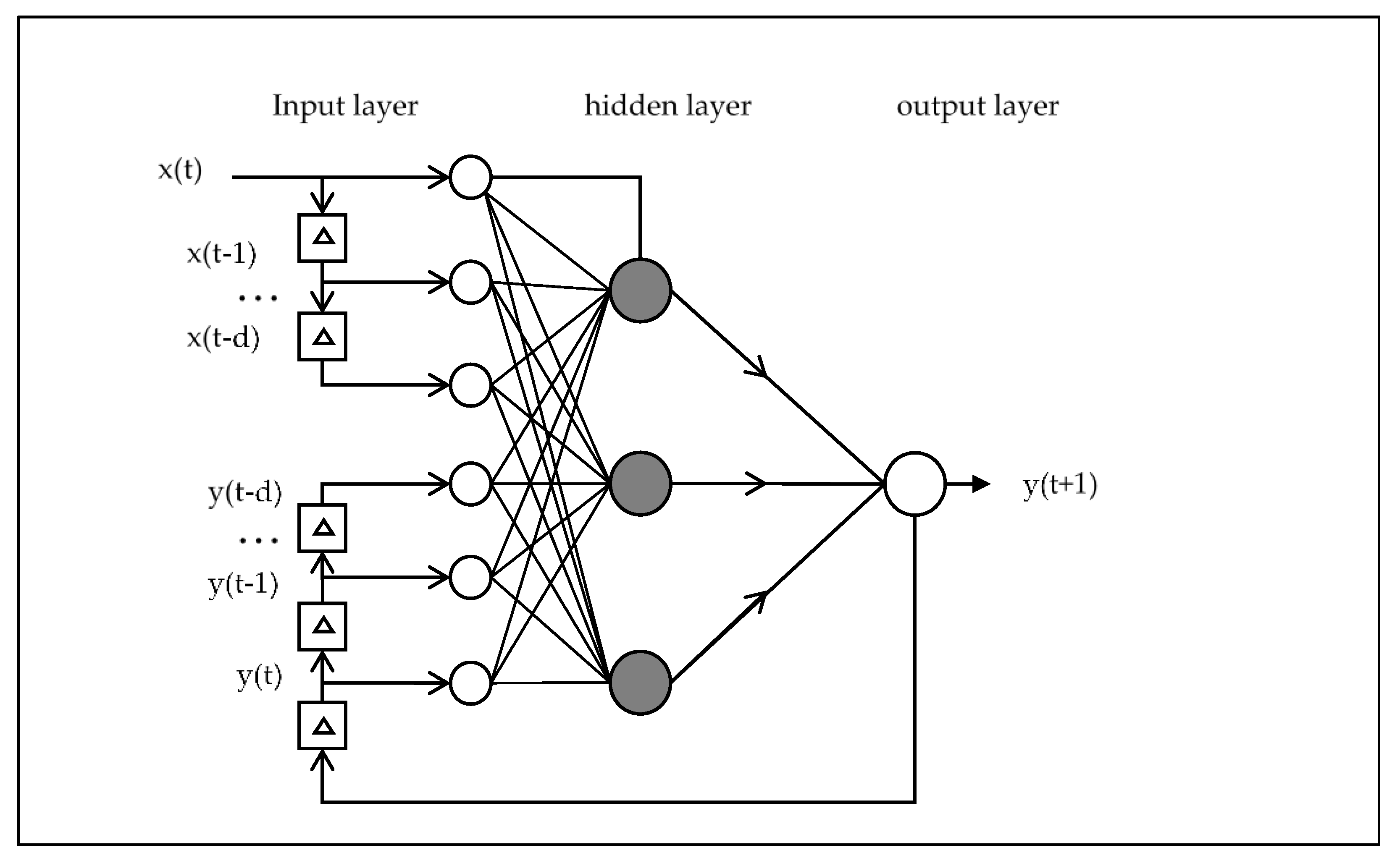
Figure 1. Nonlinear autoregressive exogenous network architecture.
Symmetry 09 00283 g001
Figure 2. Output response (highlighting data division method).
Symmetry 09 00283 g002
Figure 3. Apple stock graph.
Symmetry 09 00283 g003
Figure 4. Sunspot numbers graph.
Symmetry 09 00283 g004
Figure 5. Santa Fe laser graph.
Symmetry 09 00283 g005
Figure 6. Istanbul stock data graph.
Symmetry 09 00283 g006
Figure 7. Empirical mode decomposition of the Istanbul stock data (ISE) [5].
Symmetry 09 00283 g007
Figure 8. Non-linear autoregressive exogenous neural network–empirical mode decomposition (NARX-EMD)v2: Hierarchical meta-learning using the EMDdenoiseV2 algorithm.
Symmetry 09 00283 g008
Figure 9. EMD comparison of SFL (a) with SOL (b).
Symmetry 09 00283 g009
Table 1. Algorithms normalized mean square error (NMSE) performance comparison on Apple stock (AAPL).
Delay Windowlag: 5lag: 10
AlgorithmNARNARX-MANARX-EMDv2NARNARX-MANARX-EMDv2
Division/ANN neurons105010501050105010501050
Avg. Training Time (s)2.1131.5512.7663.4933.0414.2692.4562.2883.1575.3943.2247.332
Avg. Training Error0.00712520.00701750.00709700.00696180.00427490.00086380.00709560.00690040.00706650.00689030.00335420.0010875
Avg. Test Error
± standard deviation
0.0016678
±0.0009144
0.0037132
±0.0011296
0.0017700
±0.0010237
0.0040955
±0.0010815
0.0007602
±0.0011614
0.0004631
±0.0003893
0.0013870
±0.0010336
0.0042773
±0.0021347
0.0014124
±0.0013610
0.0046522
±0.0020343
0.0007500
±0.0013131
0.0008448
±0.0015741
Minimum Test Error0.00035730.00096360.00044690.00225970.00005080.00007980.00037580.00153880.00044930.00196100.00004380.0000701
p-value vs. best1.81 × 10−251.87 × 10−686.71 × 10−256.34 × 10−791.67 × 10−02best1.39 × 10−145.01 × 10−422.46 × 10−109.11 × 10−503.84 × 10−022.02 × 10−02
Table 2. Algorithms NMSE performance comparison on sunspot (SOL).
Delay Windowlag: 5lag: 10
AlgorithmNARNARX-MANARX-EMDv2NARNARX-MANARX-EMDv2
Division/ANN neurons105010501050105010501050
Avg. Training Time (s)2.2551.6242.9633.8912.9573.9222.2372.32.765.582.9595.985
Avg. Training Error0.11168330.10055950.10873130.09498370.03940430.05581200.10853900.09604260.10741480.08795320.03983710.0561283
Avg. Test Error
± standard deviation
0.3913484
±0.7046393
0.8481608
±0.4306742
0.3934549
±1.1453019
0.8978903
±1.1651971
0.0974777
±0.0870907
0.6780297
±0.5060787
0.2442256
±0.0750881
0.6417264
±0.4650035
0.2905302
±0.1672015
0.6722254
±0.6007605
0.0980438
±0.0369733
0.6016824
±0.4468190
Minimum Test Error0.18835770.26960930.19318200.20584340.05539650.16431100.18863220.21166810.18049970.19797360.06099810.1521699
p-value vs. best5.60 × 10−051.49 × 10−401.11 × 10−021.10 × 10⁻¹⁰best5.12 × 10−232.05 × 10−271.30 × 10−237.19 × 10−201.20 × 10−179.53 × 10−012.48 × 10⁻²²
Table 3. Algorithms NMSE performance comparison on Santa Fe laser (SFL).
Delay Windowlag: 5lag: 10
AlgorithmNARNARX-MANARX-EMDv2NARNARX-MANARX-EMDv2
Division/ANN neurons105010501050105010501050
Avg. Training Time (s)1.6220.9931.7203.4491.2104.0191.5462.3662.4824.9591.4914.194
Avg. Training Error0.01324330.02255470.02376470.00179280.06668830.01210780.01060710.00040860.02176370.00047890.04911240.0090752
Avg. Test Error
± standard deviation
0.0043834
±0.0140755
0.0037581
±0.0022762
0.0115036
±0.0677390
0.0009243
±0.0018475
0.0298414
±0.0555601
0.0083077
±0.0398612
0.0041026
±0.0108263
0.0004567
±0.0001875
0.0052185
±0.0094118
0.0004919
±0.0003914
0.0264680
±0.0613395
0.0057052
±0.0298941
Minimum Test Error0.00072380.00173720.00047520.00031550.00201930.00085170.00031110.00028700.00027300.00027460.00068130.0003910
p-value vs. best6.04 × 10−031.39 × 10−321.06 × 10−011.30 × 10−023.68 × 10−075.14 × 10−029.66 × 10−04best1.08 × 10−064.21 × 10−013.73 × 10−058.22 × 10−02
Table 4. Algorithms NMSE performance comparison on Istanbul Stock Exchange (ISE).
Delay Windowlag: 5lag: 10
AlgorithmNARNARX-MANARX-EMDv2NARNARX-MANARX-EMDv2
Division/ANN neurons105010501050105010501050
Avg. Training Time (s)0.6160.4510.6370.7970.6820.7480.5910.6670.6401.0770.5911.032
Avg. Training Error1.04668280.87956381.03666500.88665560.55779680.74281101.04801040.84586511.00994250.81499230.60013500.8643662
Avg. Test Error
± standard deviation
0.8579863
±0.0516803
0.9902402
±0.1252702
0.8677769
±0.0810234
0.9540938
±0.1115357
0.4721791
±0.1063513
1.0481726
±0.2227919
0.7809116
±0.0359027
0.9983421
±0.1287332
0.7878874
±0.0559552
0.8587937
±0.0783127
0.4165572
±0.0513170
0.8576149
±0.0742370
Minimum Test Error0.77072210.80268800.76343480.81741380.33356020.76996300.71521550.78547050.68347710.70916680.33181210.7032872
p-value vs. best2.20 × 10−1297.32 × 10−1014.92 × 10−1092.15 × 10−1035.16 × 10−061.64 × 10−694.78 × 10−1263.92 × 10−1004.19 × 10−1122.41 × 10−109best4.79 × 10−112