
Computing the Surface Area of Three-Dimensional Scanned Human Data


Abstract
:
1. Introduction
- We propose a simple and effective area computation method based on surface reconstruction for the body parts of 3D scanned human models.
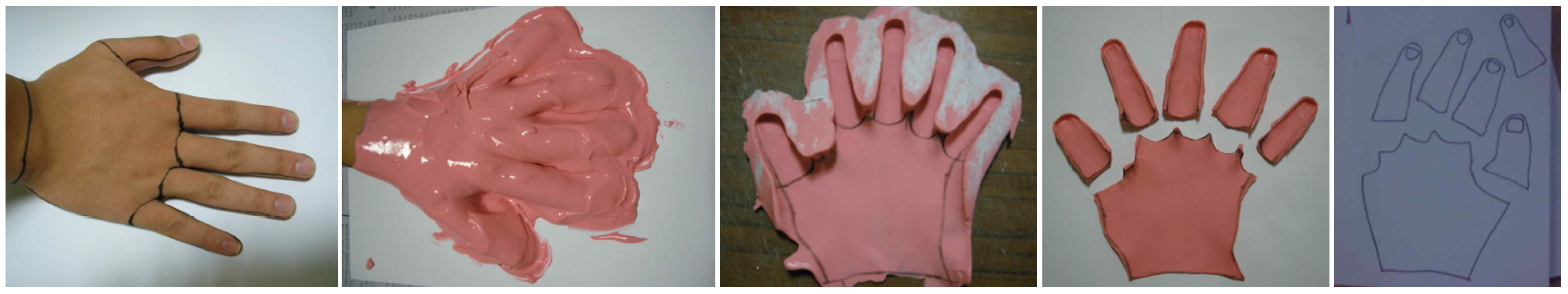
- The area computed using the surface reconstruction method has a 95% similarity with that obtained by using the traditional alginate method.
- Our area computation method proves to be a possible substitute for the cumbersome alginate method.
2. Related Work
3. Computing the Surface Area of 3D Scanned Human Data
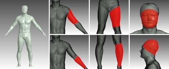
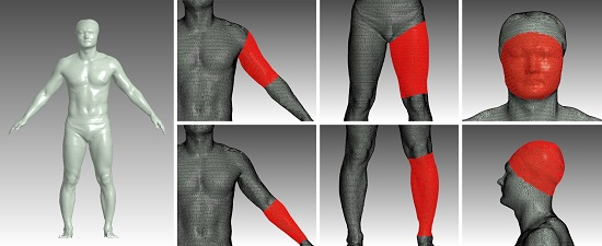
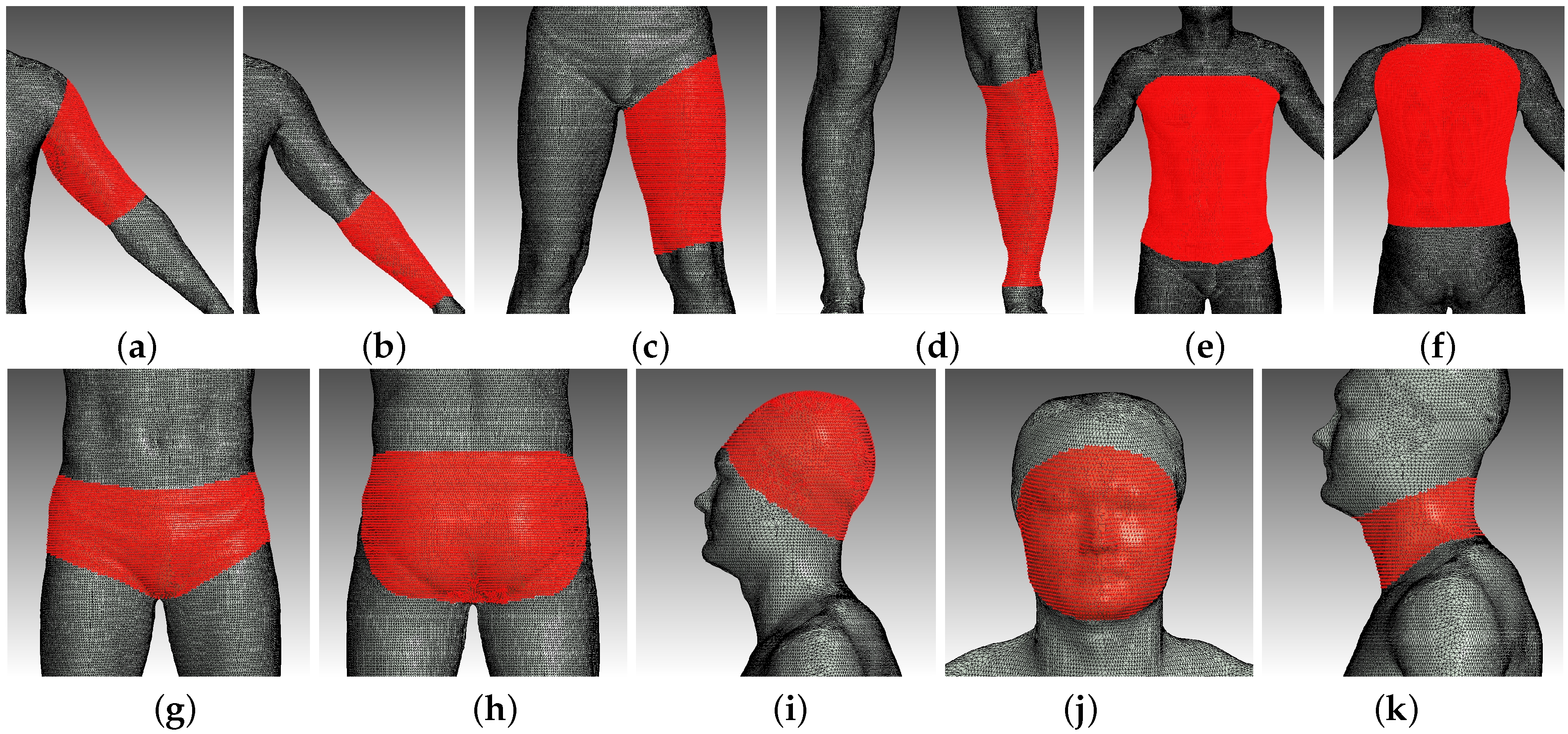
3.1. Natural User Interface for Selecting the Region of Interest
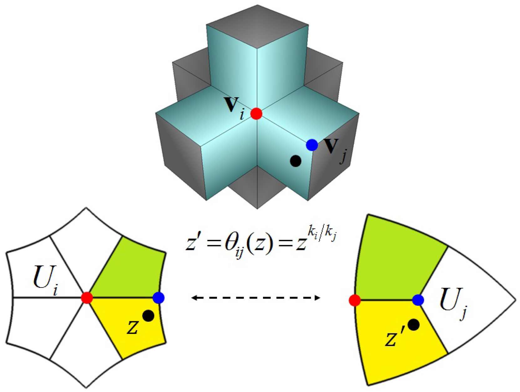
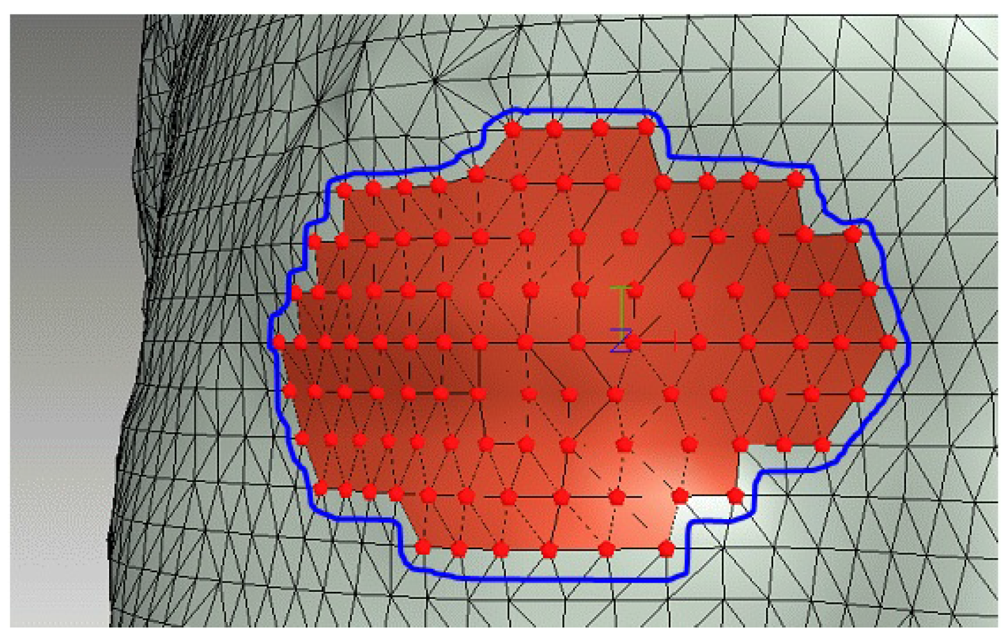
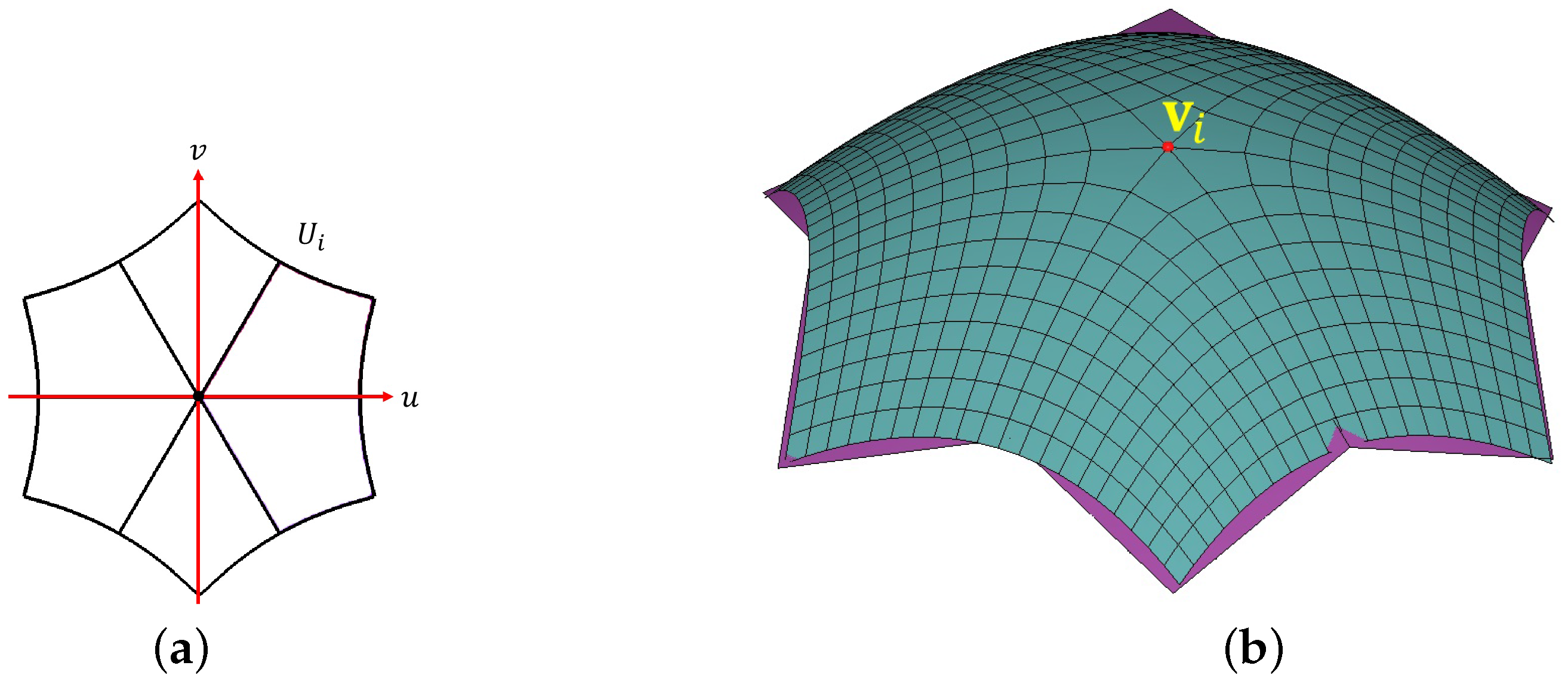
3.2. Smooth Surface Reconstruction
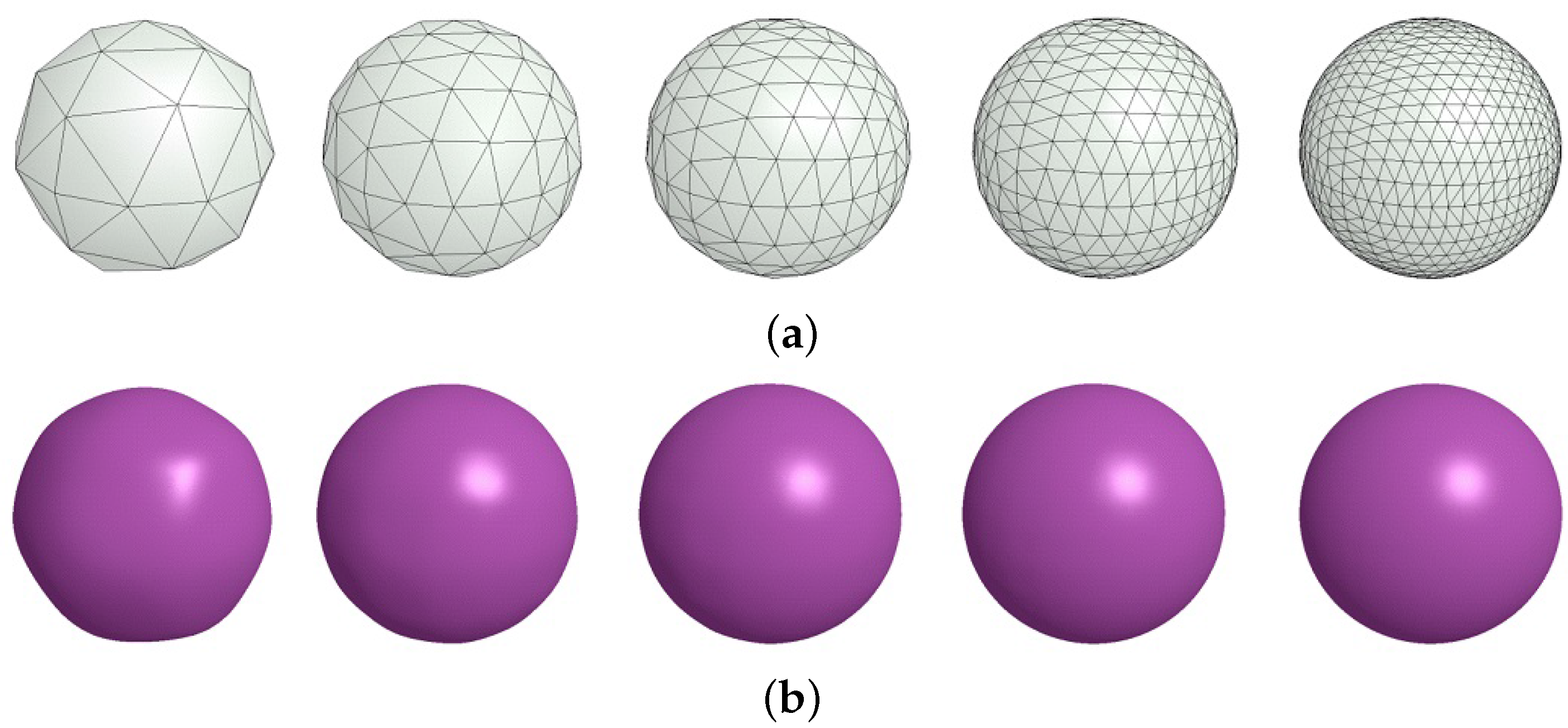
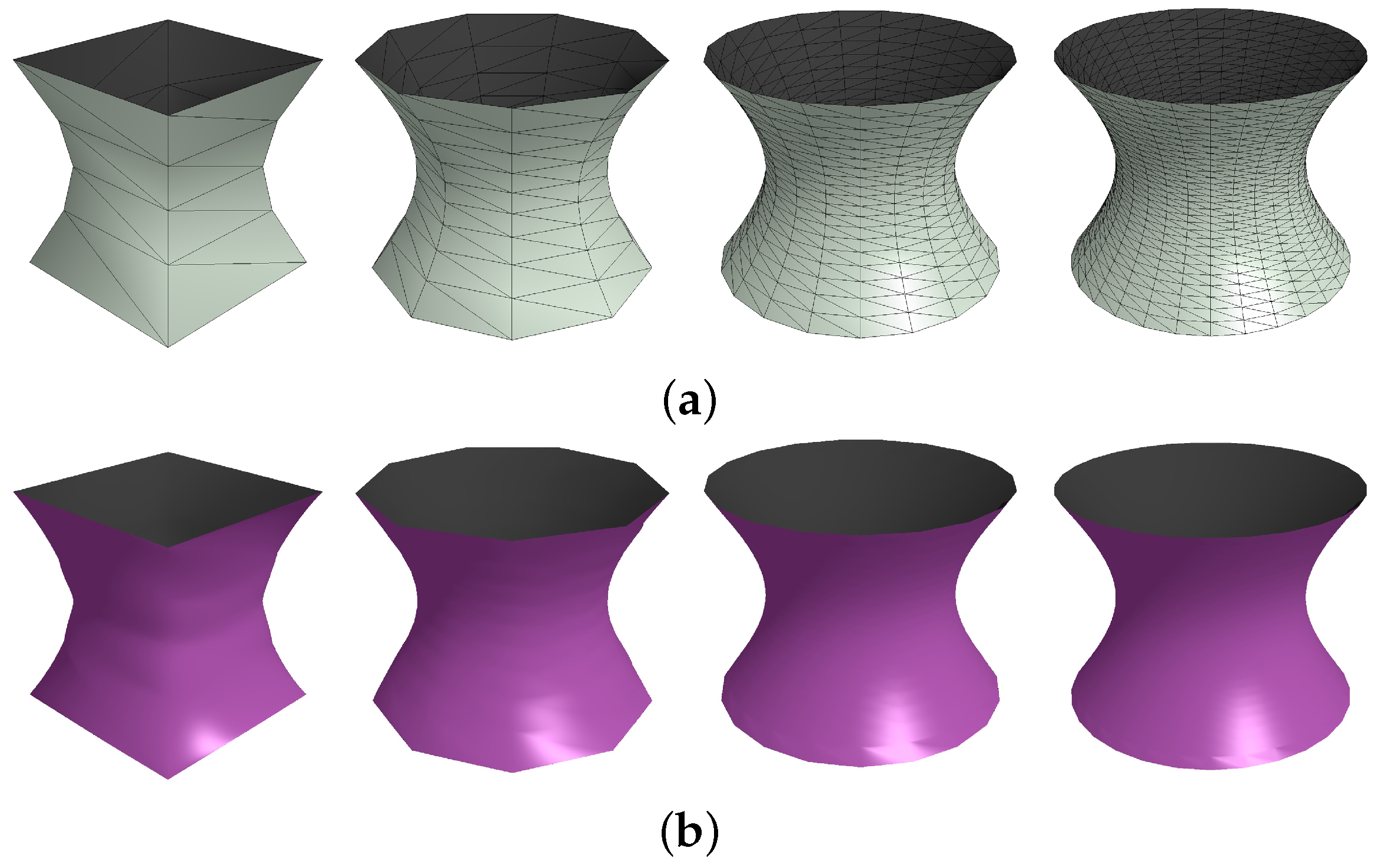
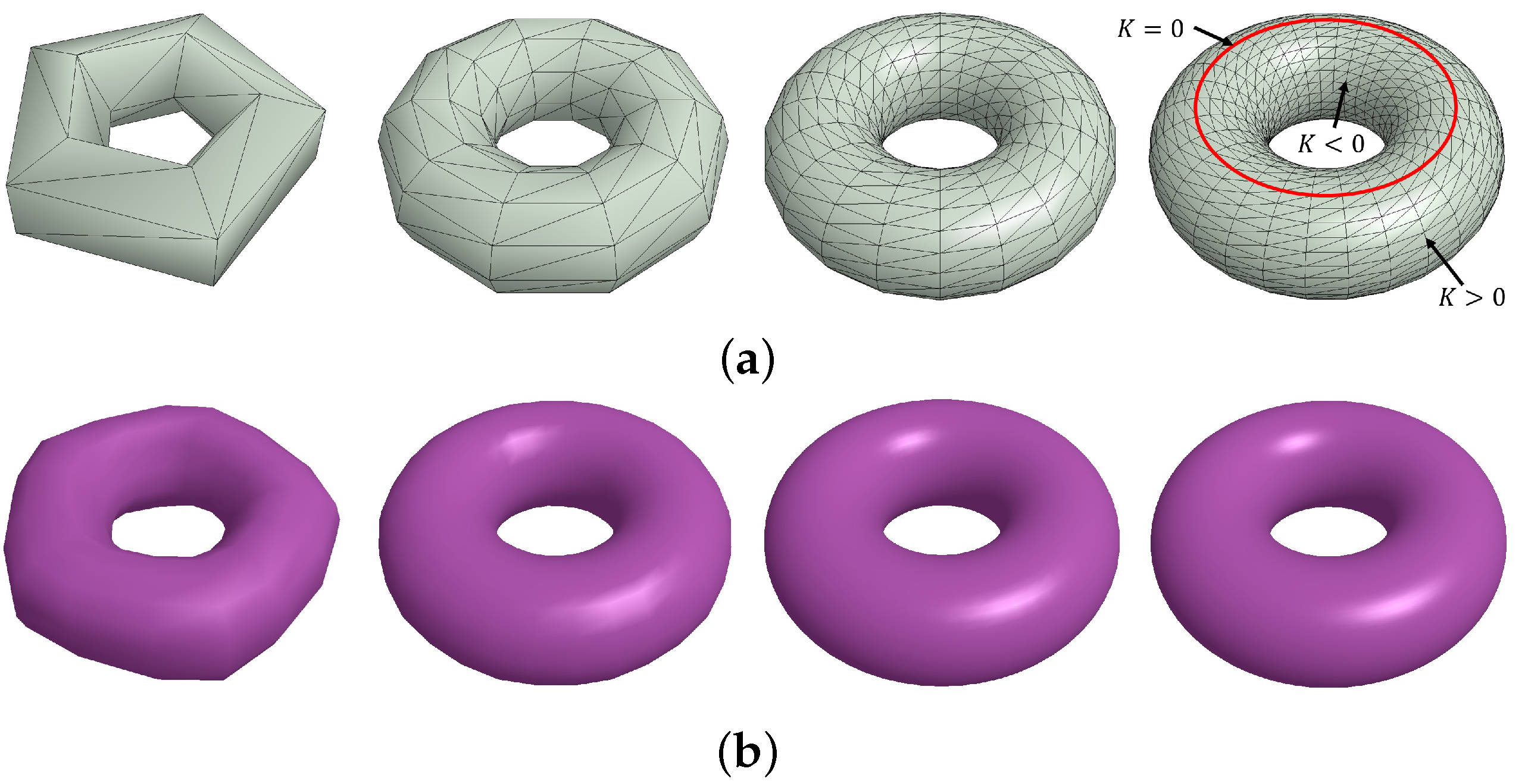
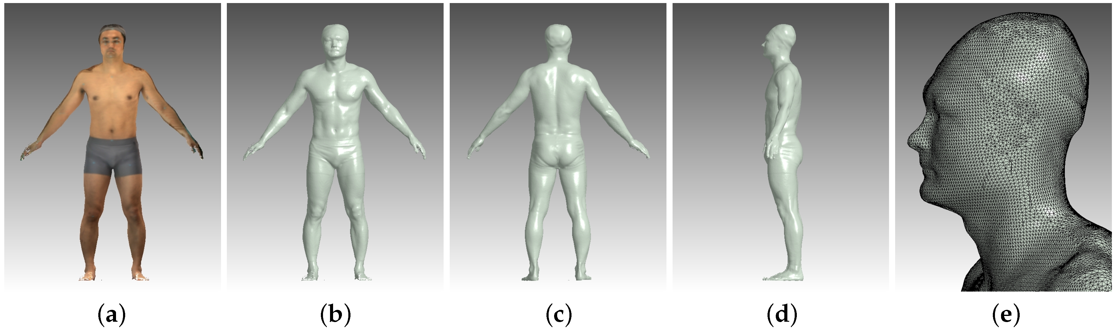
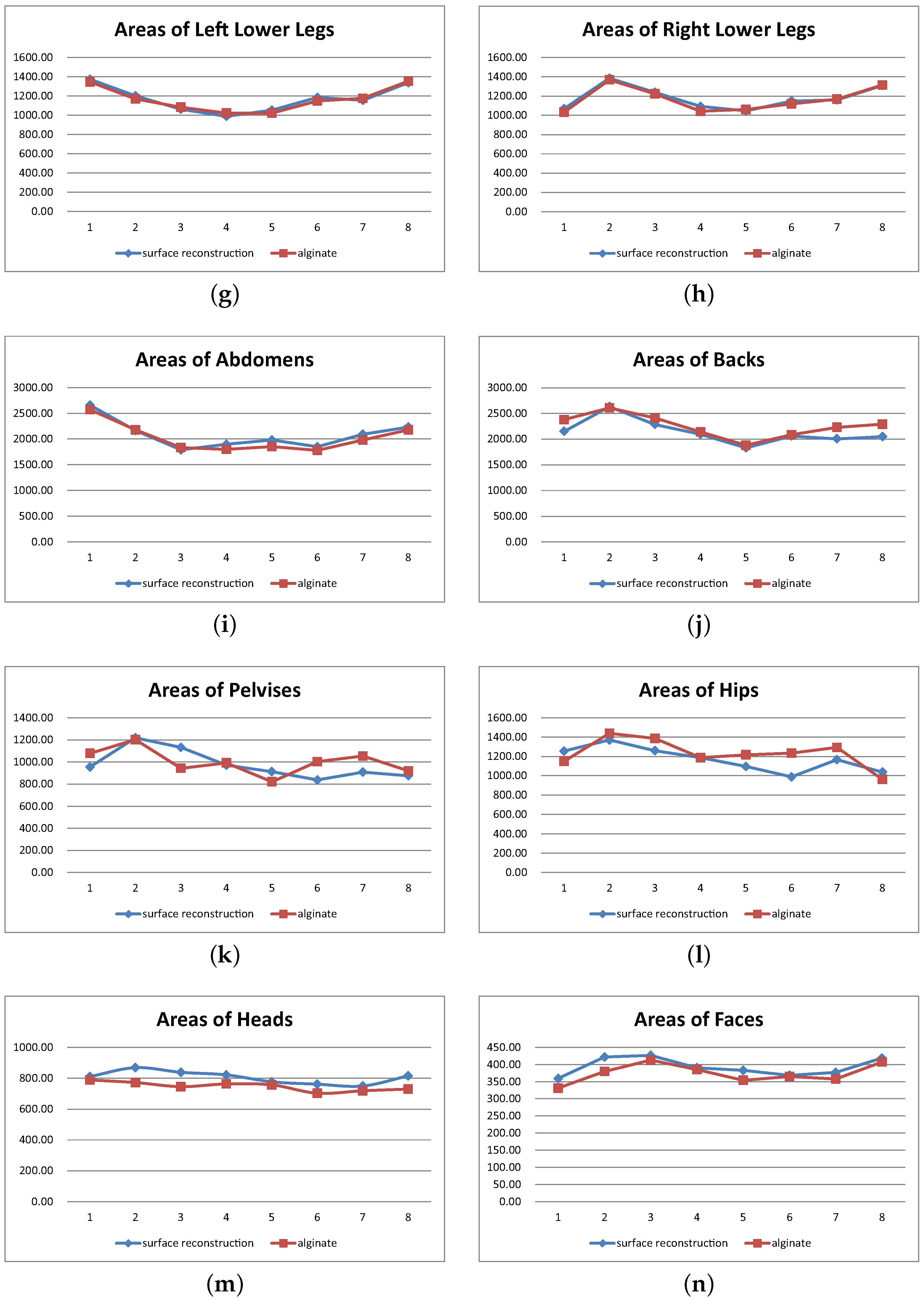
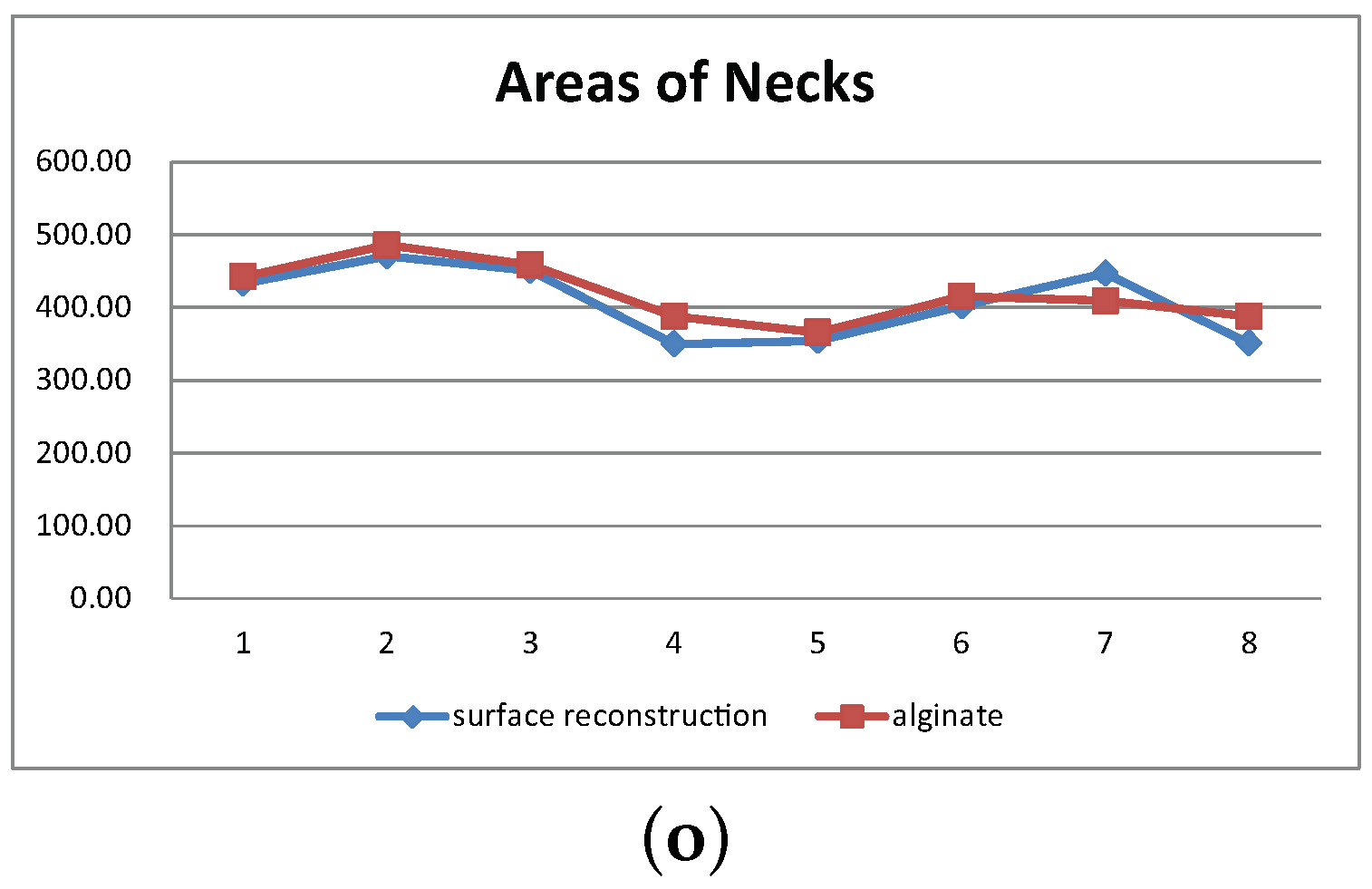
4. Experimental Results
5. Conclusions
Acknowledgments
Author Contributions
Conflicts of Interest
References
- Lee, K.Y.; Mooney, D.J. Alginate: Properties and biomedical applications. Prog. Polym. Sci. 2012, 37, 106–126. [Google Scholar] [CrossRef] [PubMed]
- 3D Geomagic. Available online: http://www.geomagic.com/en/products/capture/overview (accessed on 16 March 2016).
- Whole Body 3D Scanner (WBX). Available online: http://cyberware.com/products/scanners/wbx.html (accessed on 16 March 2016).
- LaserDesign. Available online: http://www.laserdesign.com/products/category/3d-scanners/ (accessed on 16 March 2016).
- TRIOS. Available online: http://www.3shape.com/ (accessed on 16 March 2016).
- Exocad. Available online: http://exocad.com/ (accessed on 16 March 2016).
- Tikuisis, P.; Meunier, P.; Jubenville, C. Human body surface area: Measurement and prediction using three dimensional body scans. Eur. J. Appl. Physiol. 2001, 85, 264–271. [Google Scholar] [CrossRef] [PubMed]
- Yu, C.Y.; Lo, Y.H.; Chiou, W.K. The 3D scanner for measuring body surface area: A simplified calculation in the Chinese adult. Appl. Ergon. 2003, 34, 273–278. [Google Scholar] [CrossRef]
- Yu, C.Y.; Lin, C.H.; Yang, Y.H. Human body surface area database and estimation formula. Burns 2010, 36, 616–629. [Google Scholar] [CrossRef] [PubMed]
- Lee, J.Y.; Choi, J.W. Comparison between alginate method and 3D whole body scanning in measuring body surface area. J. Korean Soc. Cloth. Text. 2005, 29, 1507–1519. [Google Scholar]
- Vlachos, A.; Peters, J.; Boyd, C.; Mitchell, J.L. Curved PN Triangles. In Proceedings of the 2001 Symposium on Interactive 3D Graphics (I3D ’01), Research Triangle Park, NC, USA, 19–21 March 2001; ACM: New York, NY, USA, 2001; pp. 159–166. [Google Scholar]
- Vida, J.; Martin, R.; Varady, T. A survey of blending methods that use parametric surfaces. Computer-Aided Des. 1994, 26, 341–365. [Google Scholar] [CrossRef]
- Choi, B.; Ju, S. Constant-radius blending in surface modeling. Computer-Aided Des. 1989, 21, 213–220. [Google Scholar] [CrossRef]
- Lukács, G. Differential geometry of G1 variable radius rolling ball blend surfaces. Computer-Aided Geom. Des. 1998, 15, 585–613. [Google Scholar] [CrossRef]
- Hartmann, E. Parametric Gn blending of curves and surfaces. Vis. Comput. 2001, 17, 1–13. [Google Scholar] [CrossRef]
- Song, Q.; Wang, J. Generating Gn parametric blending surfaces based on partial reparameterization of base surfaces. Computer-Aided Des. 2007, 39, 953–963. [Google Scholar] [CrossRef]
- Grimm, C.M.; Hughes, J.F. Modeling Surfaces of Arbitrary Topology Using Manifolds. In Proceedings of the 22nd Annual Conference on Computer Graphics and Interactive Techniques (Siggraph ’95), Los Angeles, CA, USA, 6–11 August 1995; ACM: New York, NY, USA, 1995; pp. 359–368. [Google Scholar]
- Cotrina-Navau, J.; Pla-Garcia, N. Modeling surfaces from meshes of arbitrary topology. Computer-Aided Geom. Des. 2000, 17, 643–671. [Google Scholar] [CrossRef]
- Cotrina-Navau, J.; Pla-Garcia, N.; Vigo-Anglada, M. A Generic Approach to Free Form Surface Generation. In Proceedings of the Seventh ACM Symposium on Solid Modeling and Applications (SMA ’02), Saarbrucken, Germany, 17–21 June 2002; ACM: New York, NY, USA, 2002; pp. 35–44. [Google Scholar]
- Ying, L.; Zorin, D. A simple manifold-based construction of surfaces of arbitrary smoothness. ACM Trans. Graph. 2004, 23, 271–275. [Google Scholar] [CrossRef]
- Yoon, S.H. A Surface Displaced from a Manifold. In Proceedings of Geometric Modeling and Processing (GMP 2006), Pittsburgh, PA, USA, 26–28 July 2006; Springer: New York, NY, USA, 2006; pp. 677–686. [Google Scholar]
- Vecchia, G.D.; Jüttler, B.; Kim, M.S. A construction of rational manifold surfaces of arbitrary topology and smoothness from triangular meshes. Computer-Aided Geom. Des. 2008, 29, 801–815. [Google Scholar] [CrossRef]
- Vecchia, G.D.; Jüttler, B. Piecewise Rational Manifold Surfaces with Sharp Features. In Proceedings of the 13th IMA International Conference on Mathematics of Surfaces XIII, York, UK, 7–9 September 2009; pp. 90–105.
- Tomas, A.; Eric, H. Real-Time Rendering; AK Peters: Natick, MA, USA, 2002. [Google Scholar]
- Farin, G. Curves and Surfaces for CAGD: A Practical Guide, 5th ed.; Morgan Kaufmann: Burlington, MA, USA, 2002. [Google Scholar]


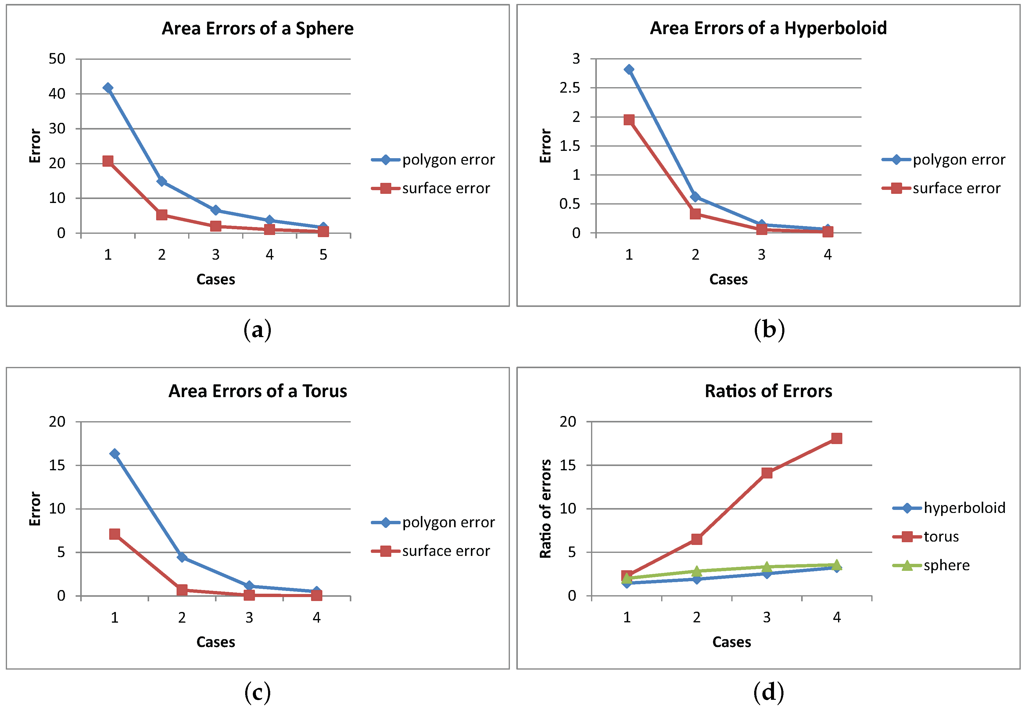
| Cases | # of Triangles | Area (time) (a) | Area (time) (b) | Error (1) | Error (2) | (1)/(2) |
|---|---|---|---|---|---|---|
| 1 | 60 | 272.46179 (0.03) | 293.46164 (3) | 41.69747 | 20.69763 | 2.01460 |
| 2 | 180 | 299.35513 (0.05) | 308.94577 (9) | 14.80413 | 5.21349 | 2.83958 |
| 3 | 420 | 307.64926 (0.06) | 312.20694 (22) | 6.510004 | 1.95233 | 3.33449 |
| 4 | 760 | 310.52105 (0.11) | 313.14139 (40) | 3.638208 | 1.01788 | 3.57431 |
| 5 | 1740 | 312.55352 (0.18) | 313.73544 (92) | 1.605738 | 0.42382 | 3.78871 |
| Cases | # of Triangles | Area (time) (a) | Area (time) (b) | Error (1) | Error (2) | (1)/(2) |
|---|---|---|---|---|---|---|
| 1 | 32 | 17.19809 (0.03) | 18.06601 (2) | 2.81723 | 1.94931 | 1.44524 |
| 2 | 162 | 19.39459 (0.05) | 19.68971 (8) | 0.62073 | 0.32561 | 1.90636 |
| 3 | 722 | 19.87309 (0.09) | 19.95923 (37) | 0.14223 | 0.05609 | 2.53575 |
| 4 | 1682 | 19.95392 (0.17) | 19.99632 (89) | 0.0614 | 0.019 | 3.23158 |
| Cases | # of Triangles | Area (time) (a) | Area (time) (b) | Error (1) | Error (2) | (1)/(2) |
|---|---|---|---|---|---|---|
| 1 | 50 | 62.64104 (0.04) | 71.86401 (3) | 16.31580 | 7.09283 | 2.30032 |
| 2 | 200 | 74.53550 (0.05) | 78.27505 (12) | 4.42134 | 0.68179 | 6.48495 |
| 3 | 800 | 77.82805 (0.1) | 78.87682 (45) | 1.12879 | 0.08002 | 14.10562 |
| 4 | 1800 | 78.45343 (0.18) | 78.92898 (98) | 0.50341 | 0.02786 | 18.06795 |
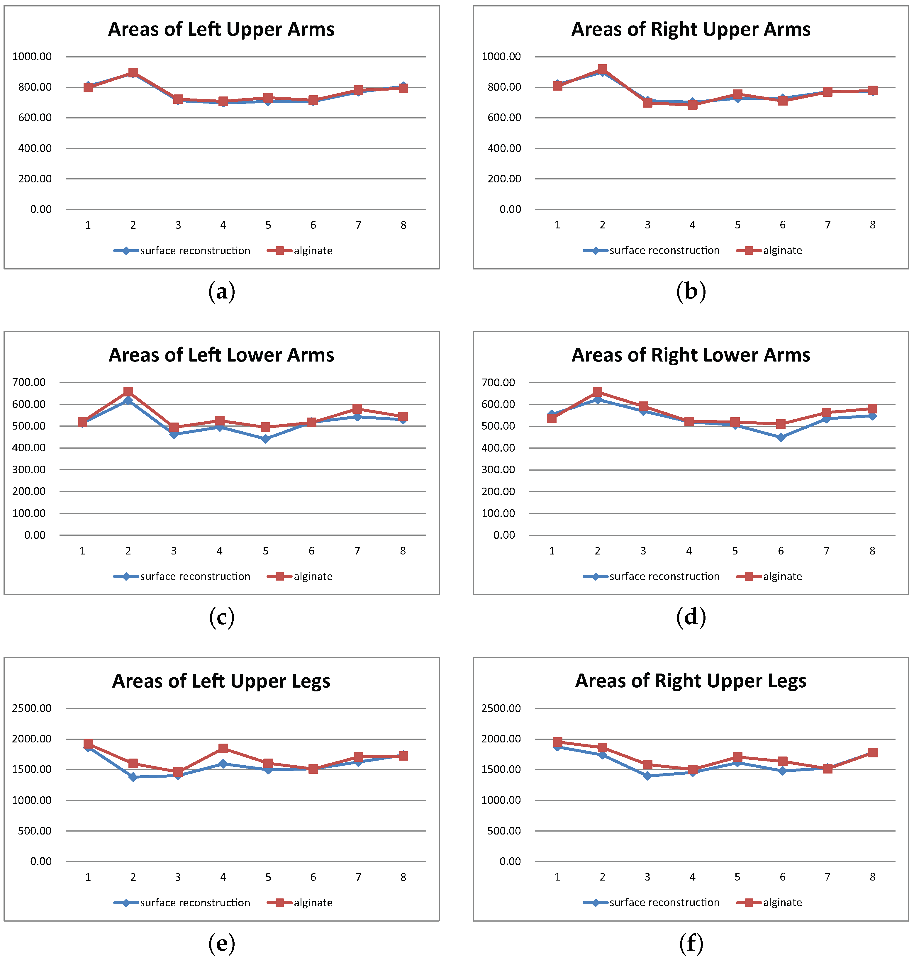
| Region | Similarity | Correlation |
|---|---|---|
| left upper arm | 0.99232920 | 0.98651408 |
| right upper arm | 0.99050425 | 0.97836923 |
| left lower arm | 0.97442492 | 0.94239832 |
| right lower arm | 0.97565553 | 0.88847152 |
| left upper leg | 0.96904881 | 0.82351873 |
| right upper leg | 0.97294687 | 0.91311208 |
| left lower leg | 0.98809628 | 0.97643038 |
| right lower leg | 0.99031974 | 0.98423465 |
| abdomen | 0.98108957 | 0.97599424 |
| back | 0.97219378 | 0.89756368 |
| pelvis | 0.94844035 | 0.50870081 |
| hips | 0.95367837 | 0.64129904 |
| head | 0.96274736 | 0.63287971 |
| neck | 0.97341437 | 0.88813431 |
| face | 0.97505372 | 0.87872788 |
| average | 0.94925100 | 0.75430084 |
© 2016 by the authors; licensee MDPI, Basel, Switzerland. This article is an open access article distributed under the terms and conditions of the Creative Commons Attribution (CC-BY) license (http://creativecommons.org/licenses/by/4.0/).
Share and Cite
Yoon, S.-H.; Lee, J. Computing the Surface Area of Three-Dimensional Scanned Human Data. Symmetry 2016, 8, 67. https://doi.org/10.3390/sym8070067
Yoon S-H, Lee J. Computing the Surface Area of Three-Dimensional Scanned Human Data. Symmetry. 2016; 8(7):67. https://doi.org/10.3390/sym8070067
Chicago/Turabian StyleYoon, Seung-Hyun, and Jieun Lee. 2016. "Computing the Surface Area of Three-Dimensional Scanned Human Data" Symmetry 8, no. 7: 67. https://doi.org/10.3390/sym8070067
APA StyleYoon, S.-H., & Lee, J. (2016). Computing the Surface Area of Three-Dimensional Scanned Human Data. Symmetry, 8(7), 67. https://doi.org/10.3390/sym8070067