
Chiral Symmetry and the Nucleon-Nucleon Interaction

Abstract
:1. Historical Perspective
2. Effective Field Theory for Low-Energy QC
If one writes down the most general possible Lagrangian, including all terms consistent with assumed symmetry principles, and then calculates matrix elements with this Lagrangian to any given order of perturbation theory, the result will simply be the most general possible S-matrix consistent with analyticity, perturbative unitarity, cluster decomposition, and the assumed symmetry principles.
- Identify the soft and hard scales, and the degrees of freedom appropriate for (low-energy) nuclear physics.
- Identify the relevant symmetries of low-energy QCD and investigate if and how they are broken.
- Construct the most general Lagrangian consistent with those symmetries and symmetry breakings.
- Design an organizational scheme that can distinguish between more and less important contributions: a low-momentum expansion.
- Guided by the expansion, calculate Feynman diagrams for the process under consideration to the desired accuracy.
2.1. Symmetries of Low-Energy QCD
2.1.1. Chiral Symmetry
2.1.2. Explicit Symmetry Breaking
2.1.3. Spontaneous Symmetry Breaking
2.2. Chiral Effective Lagrangians
3. Nuclear Forces from EFT: Overview
3.1. Chiral Perturbation Theory and Power Counting
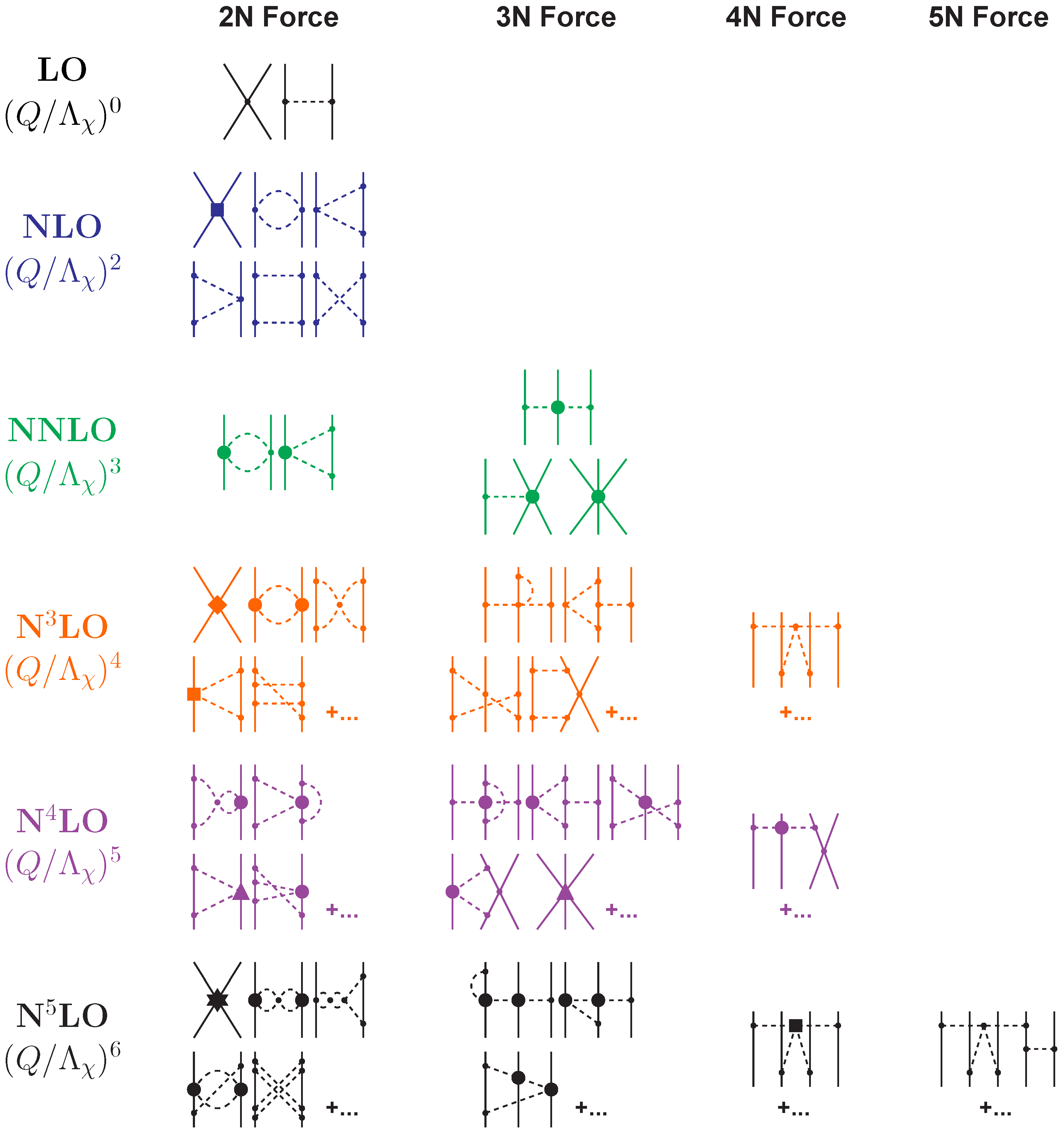
3.2. The Hierarchy of Nuclear Forces
4. Pion-Exchange Contributions to the Interaction
4.1. Leading Order (LO)
4.2. Next-to-Leading Order (NLO)
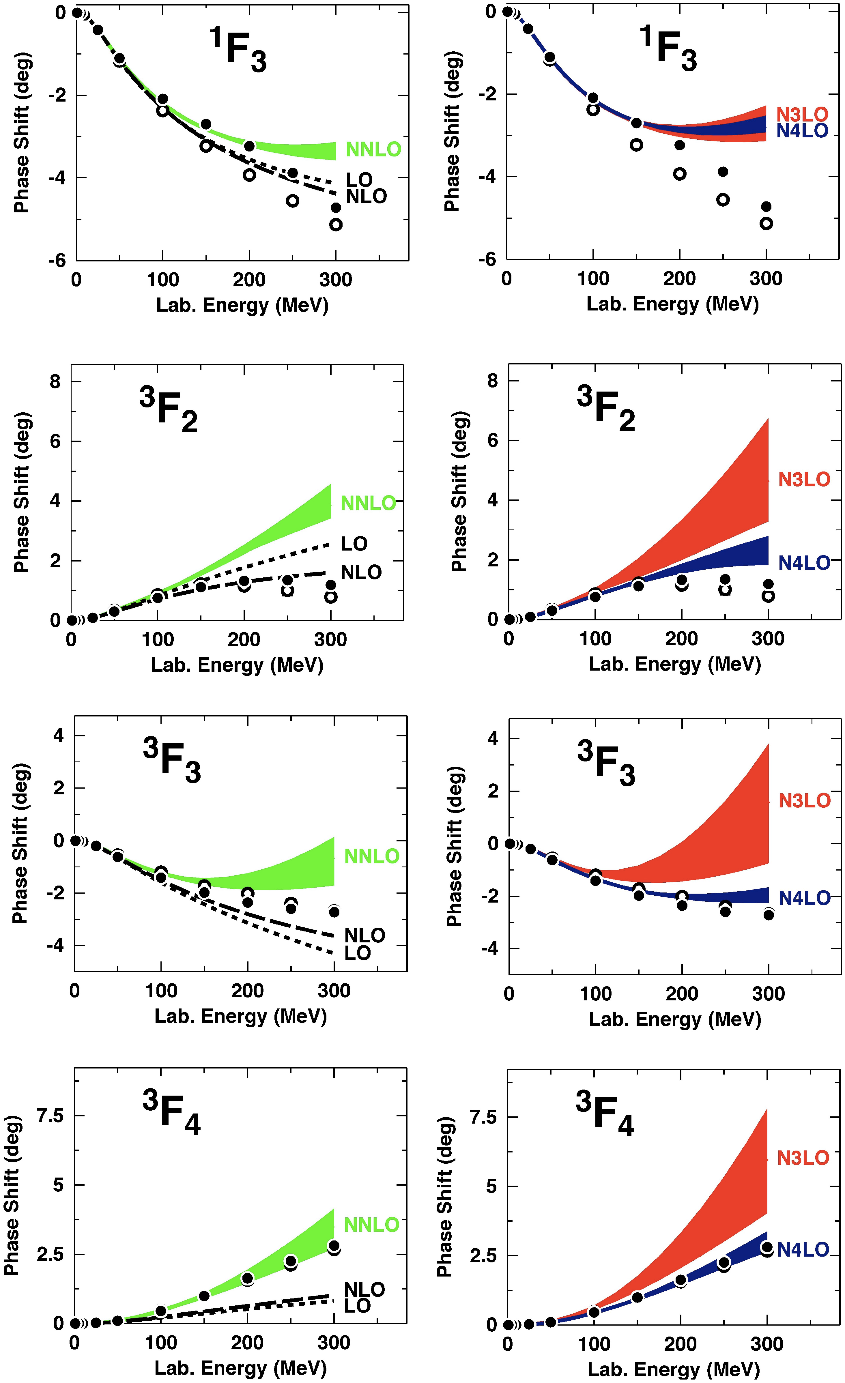
4.3. Next-to-Next-to-Leading Order (NNLO)
4.4. Next-to-Next-to-Next-to-Leading Order (NLO)
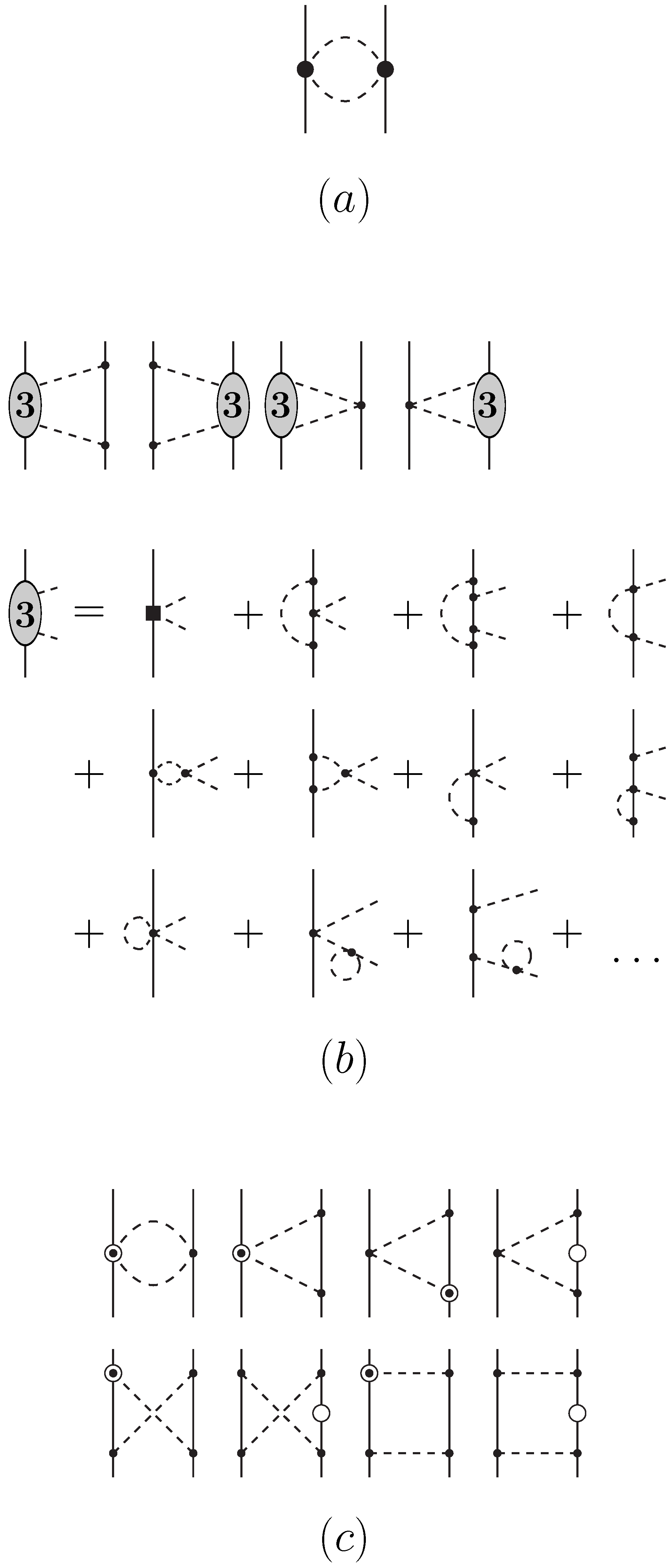
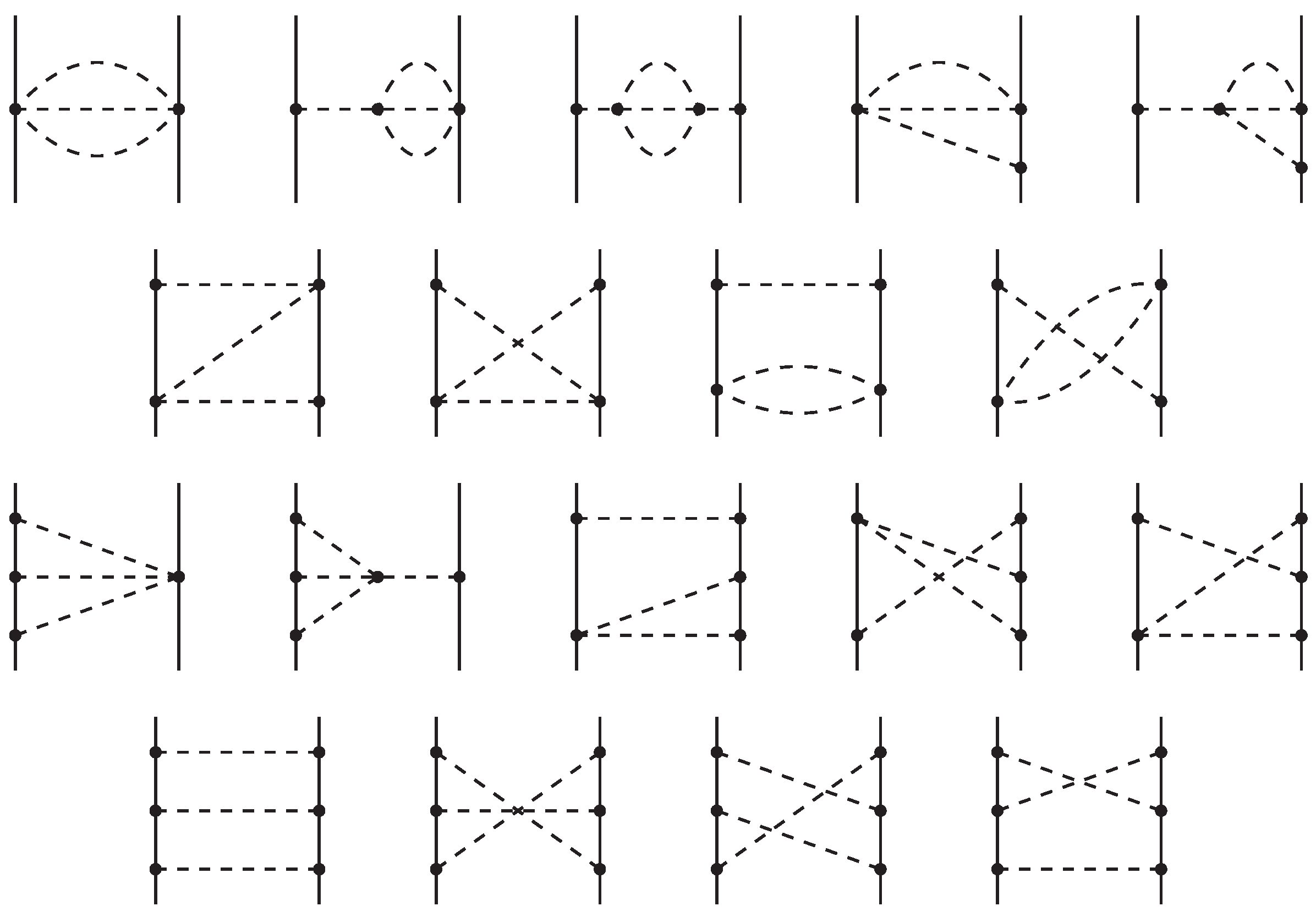
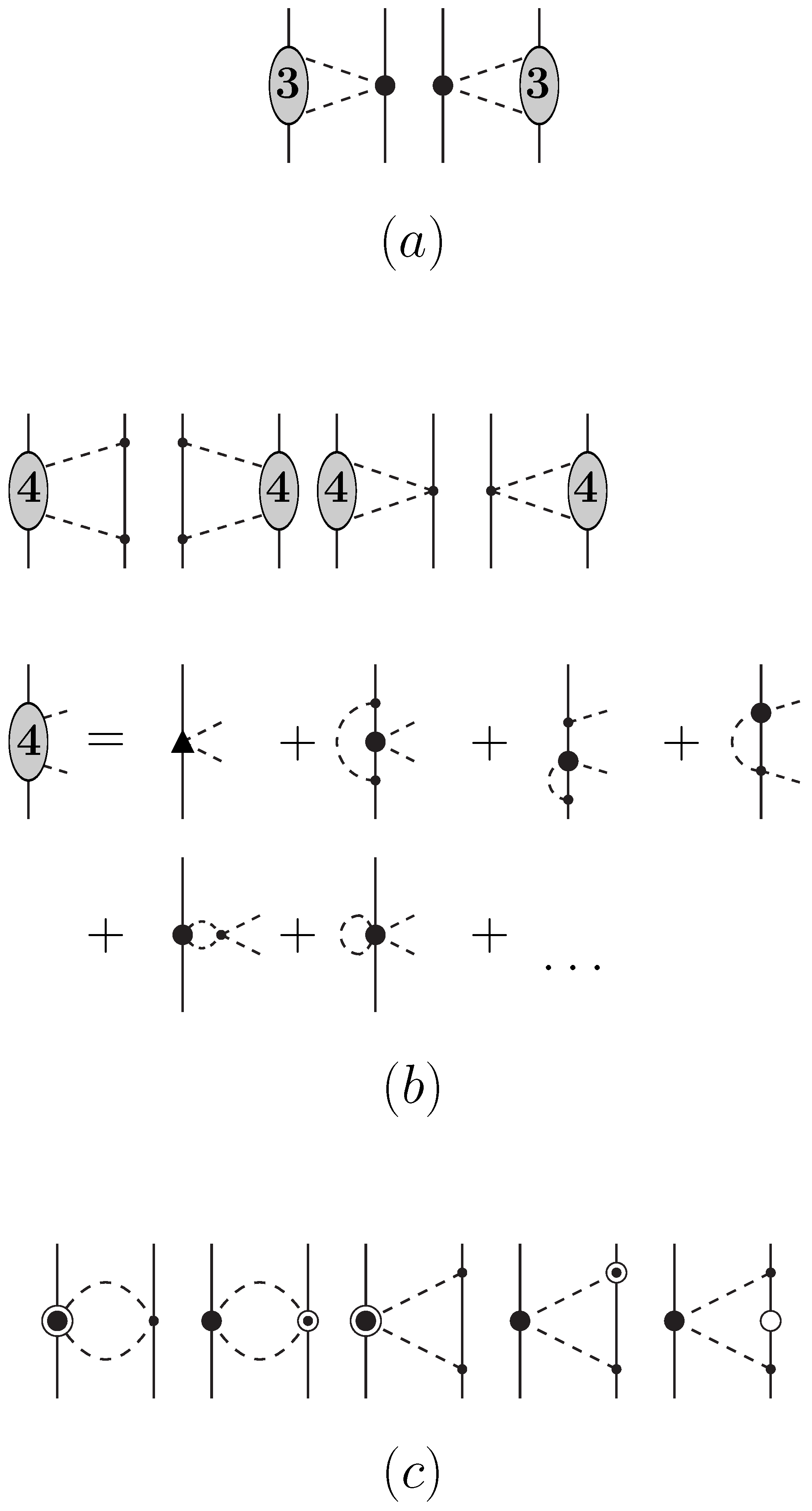
4.4.1. Football diagram at NLO
4.4.2. Leading Two-Loop Contributions
4.4.3. Leading Relativistic Corrections
4.4.4. Leading Three-Pion Exchange Contributions
4.5. Next-to-Next-to-Next-to-Next-to-Leading Order (NLO)
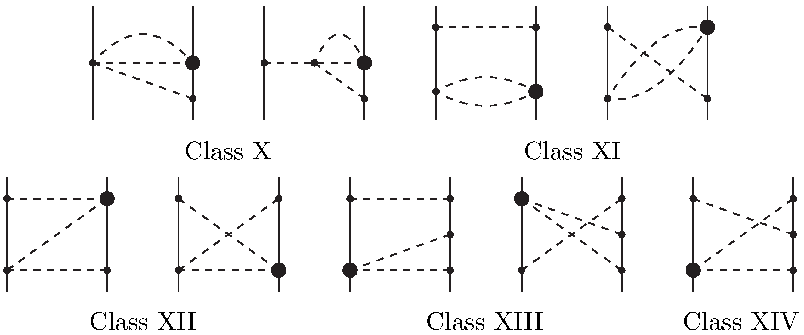
4.5.1. Two-Pion Exchange Contributions at NLO
4.5.2. Three-Pion Exchange Contributions at NLO
4.6. Next-to-Next-to-Next-to-Next-to-Next-to-Leading Order (NLO)
4.6.1. Two-Pion Exchange Contributions at NLO
4.6.2. Three-Pion Exchange Contributions at NLO
4.6.3. Four-Pion Exchange at NLO
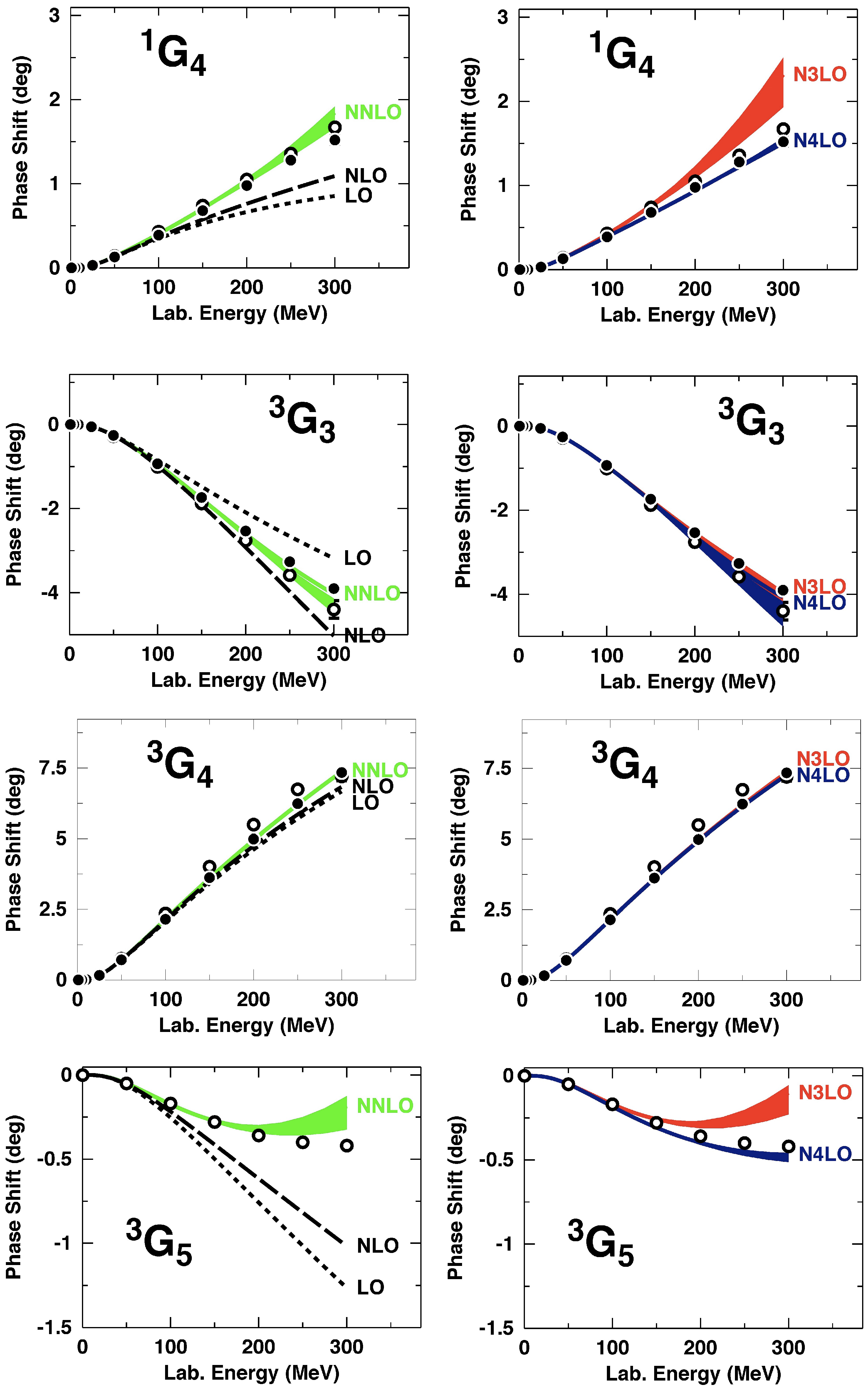
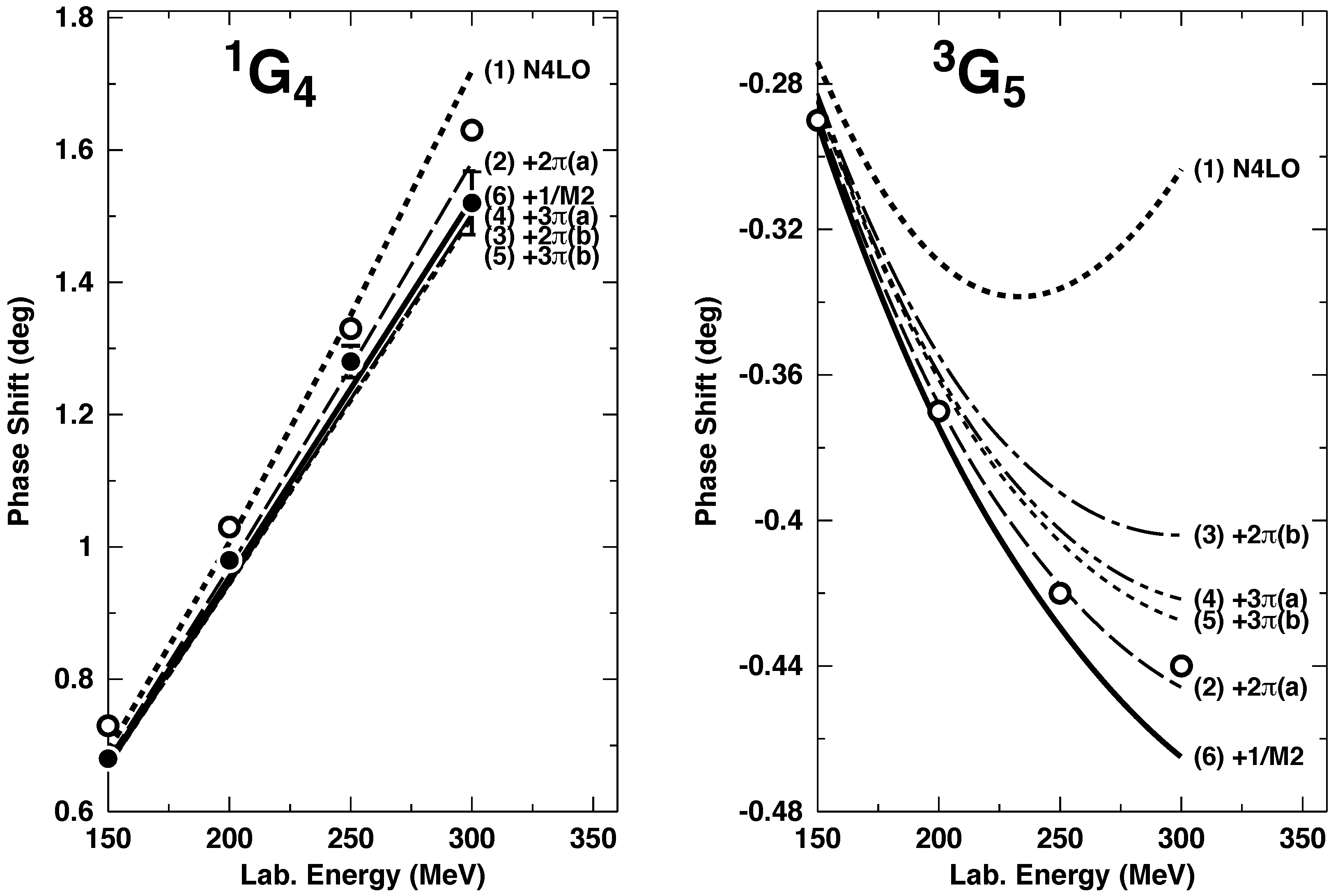
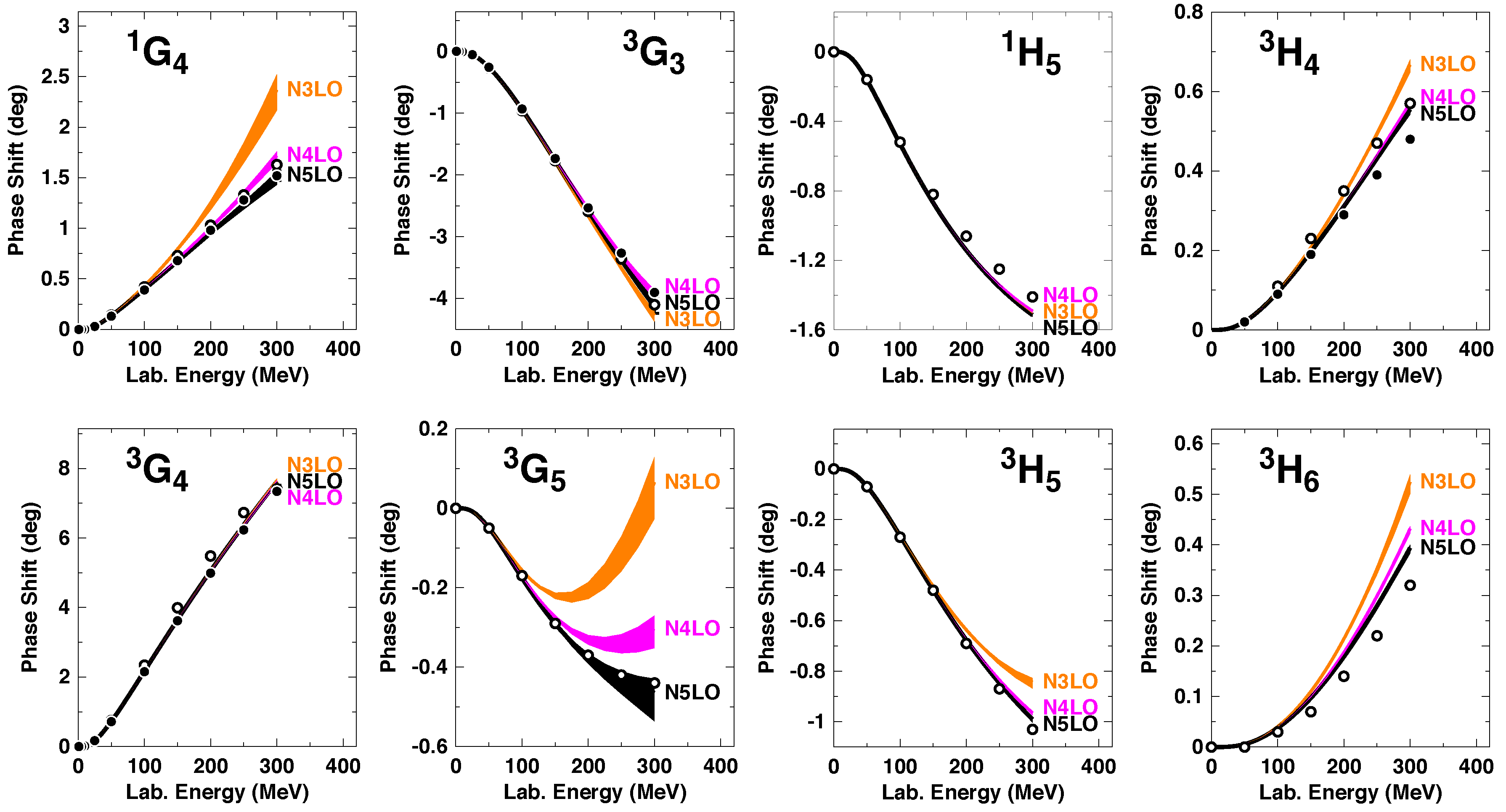
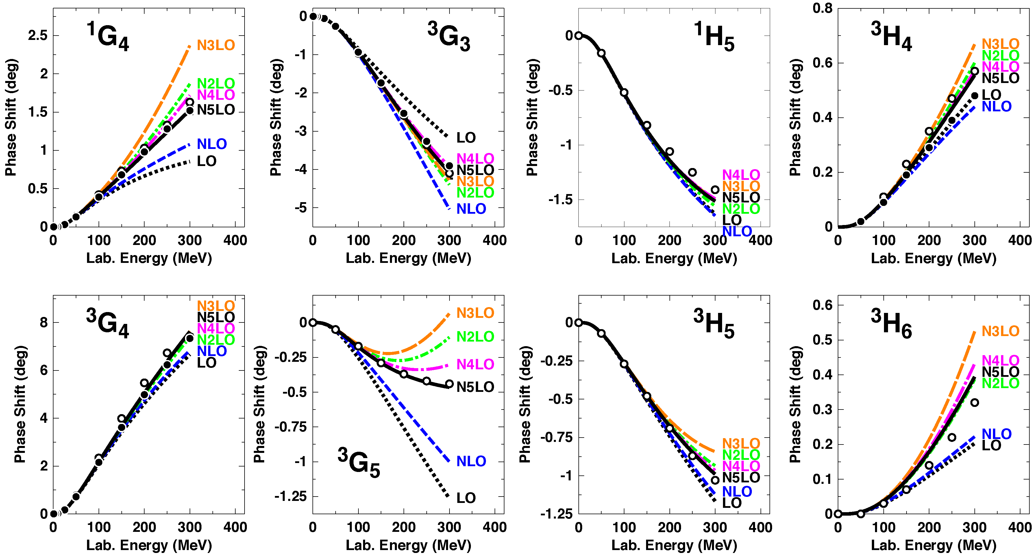
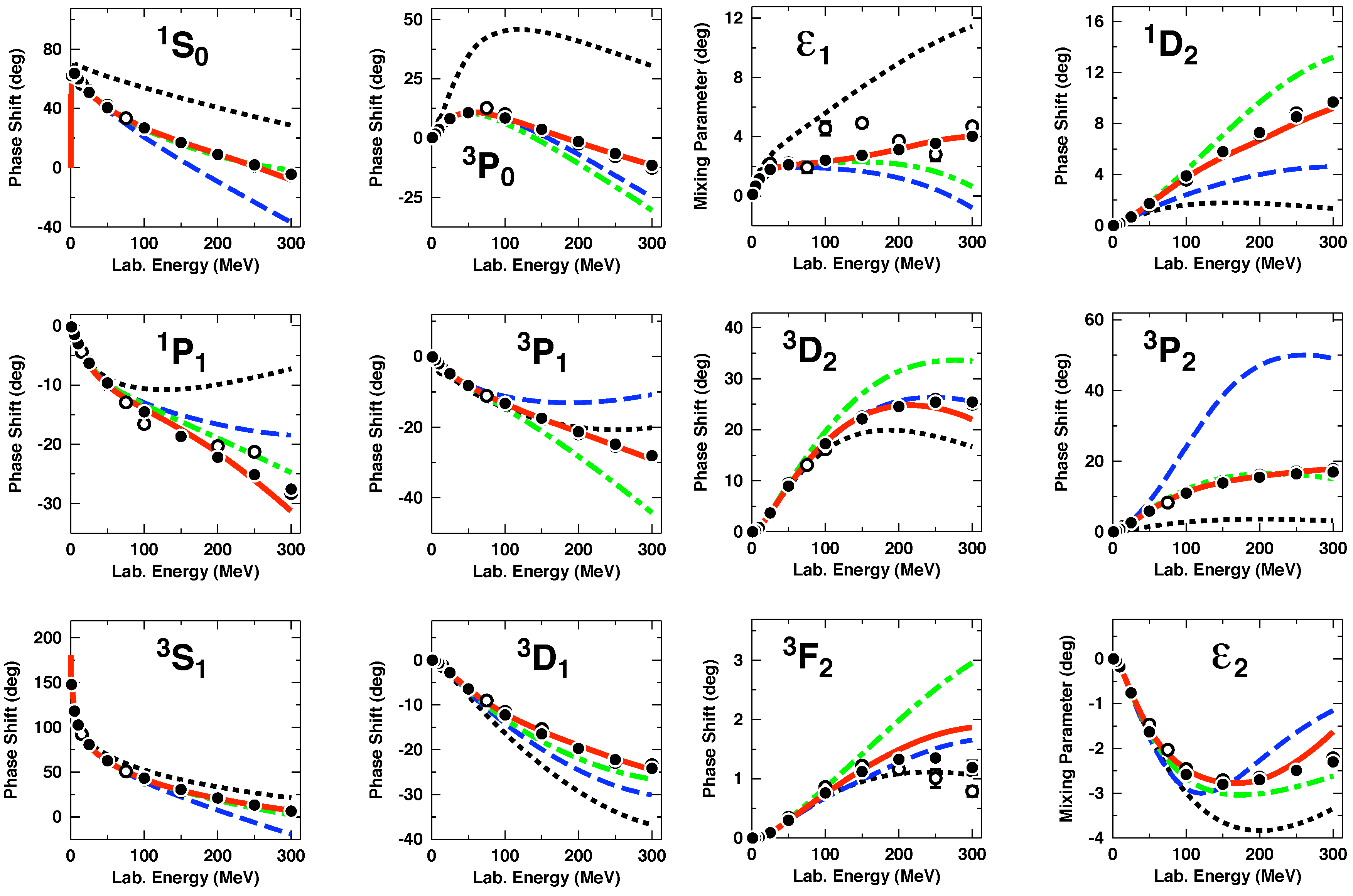
5. Perturbative Scattering in Peripheral Partial Waves
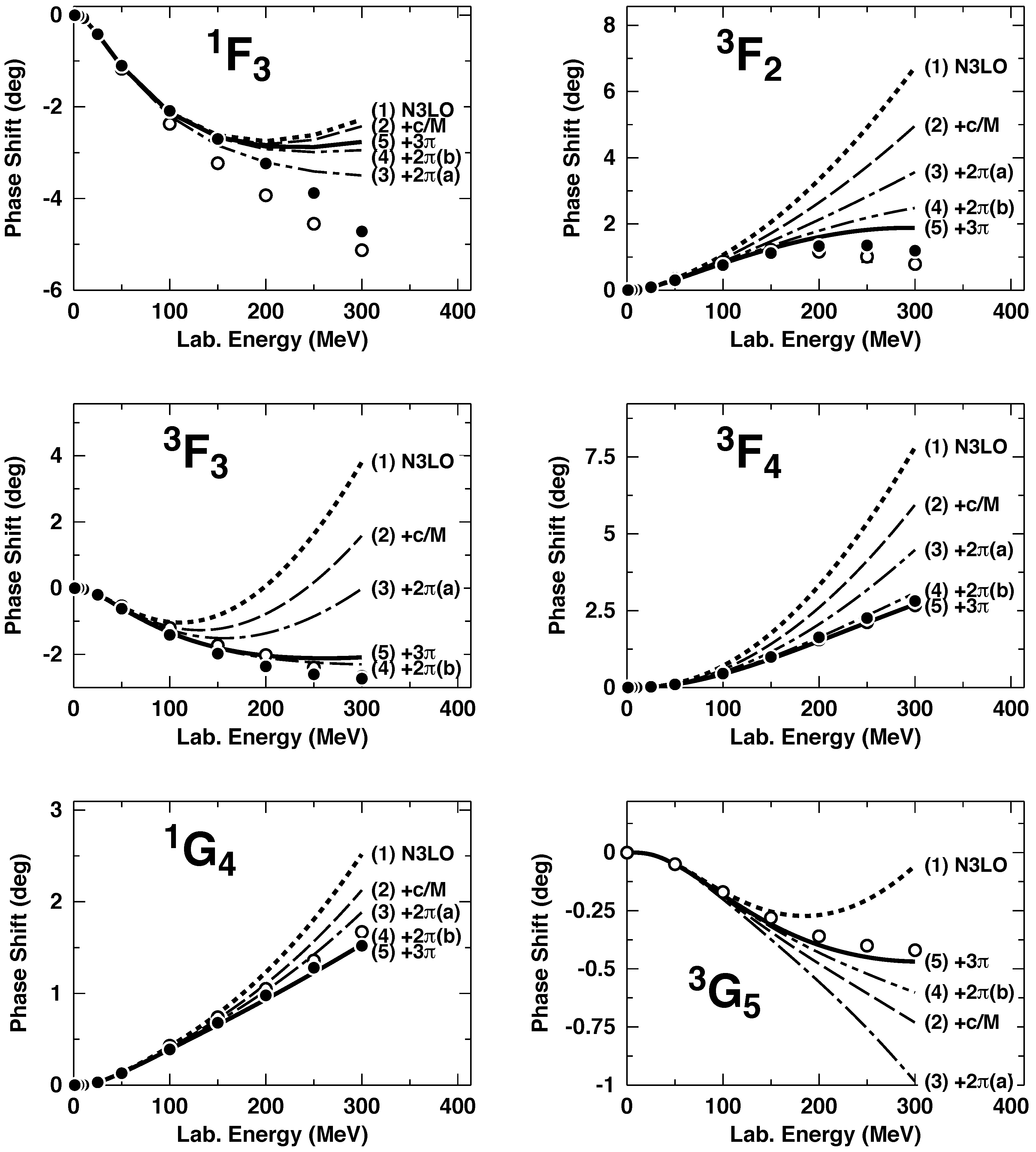
- NLO.
- The previous curve plus the corrections (denoted by “c/M”), Figure 4c.
- The previous curve plus the NLO -exchange two-loop contributions of class (a), Figure 4a.
- The previous curve plus the NLO two-loop contributions of class (b), Figure 4b.
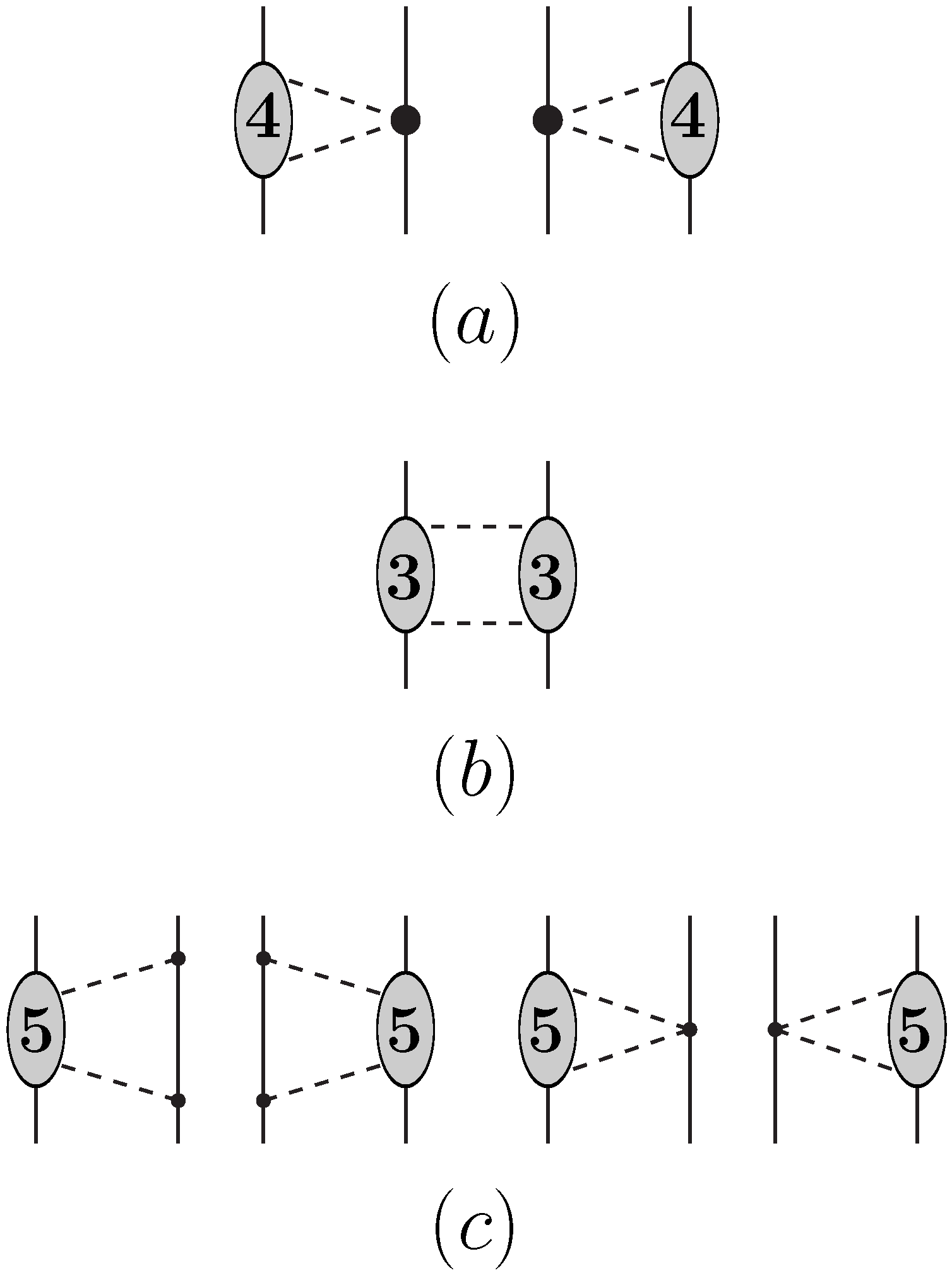
- The previous curve plus the NLO -exchange contributions, Figure 5.
- NLO.
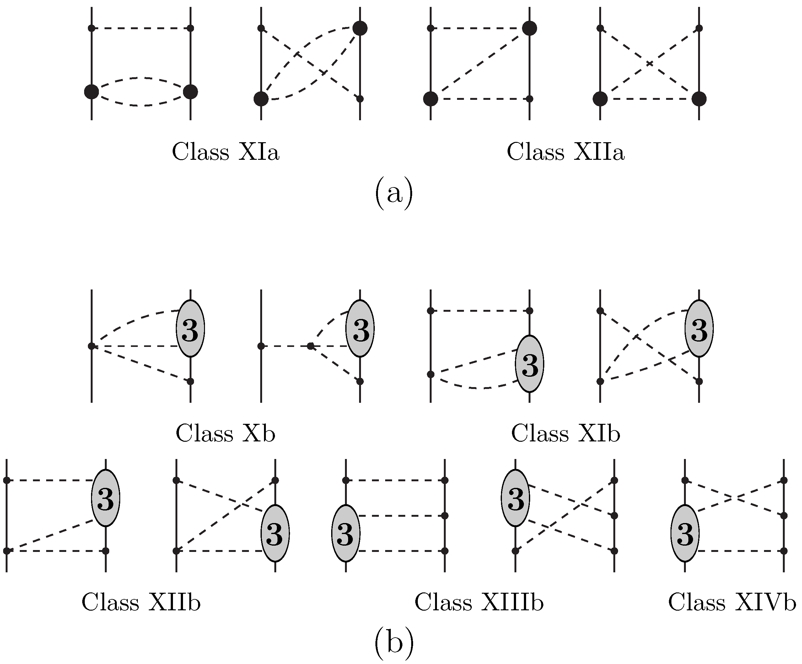
- The previous curve plus the NLO -exchange contributions of class (a), Figure 6a.
- The previous curve plus the NLO -exchange contributions of class (b), Figure 6b.
- The previous curve plus the NLO -exchange contributions of class (a), Figure 7a.
- The previous curve plus the NLO -exchange contributions of class (b), Figure 7b.
- The previous curve plus the -corrections (denoted by “1/M2”) [44].
6. Constructing Chiral Potentials
6.1. Contact Terms
6.1.1. Zeroth Order (LO)
6.1.2. Second Order (NLO)
6.1.3. Fourth Order (NLO)
6.1.4. Sixth Order (NLO)
6.2. Definition of Potential
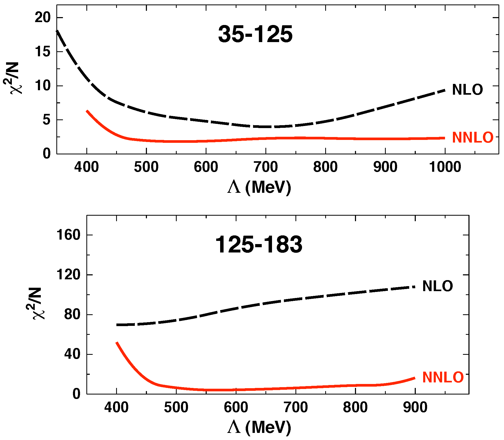
6.3. Regularization and Non-Perturbative Renormalization
6.3.1. Renormalization Beyond Leading Order
6.3.2. Back to the Beginnings
- Incorporate the correct long-range behavior: The long-range behavior of the underlying theory must be known, and it must be built into the effective theory. In the case of nuclear forces, the long-range theory is, of course, well known and given by one- and multi-pion exchanges.
- Introduce an ultraviolet cutoff to exclude high-momentum states, or, equivalent, to soften the short-distance behavior: The cutoff has two effects: First it excludes high-momentum states, which are sensitive to the unknown short-distance dynamics; only states that we understand are retained. Second it makes all interactions regular at , thereby avoiding the infinities that beset the naive approach.
- Add local correction terms (also known as contact or counter terms) to the effective Hamiltonian. These mimic the effects of the high-momentum states excluded by the cutoff introduced in the previous step. In the meson-exchange picture, the short-range nuclear force is described by heavy meson exchange, like the and . However, at low energy, such structures are not resolved. Since we must include contact terms anyhow, it is most efficient to use them to account for any heavy-meson exchange as well. The correction terms systematically remove dependence on the cutoff.
6.4. Potentials Order by Order
7. Conclusions
Acknowledgments
Conflicts of Interest
References and Notes
- Chadwick, J. The existence of a neutron. Proc. Roy. Soc. 1932, A136, 692–708. [Google Scholar] [CrossRef]
- Yukawa, H. On the interaction of elementary particles. I. Proc. Phys. Math. Soc. Jpn. 1935, 17, 48–57. [Google Scholar]
- Bryan, R.A.; Scott, B.L. Nucleon-nucleon scattering from one-boson-exchange potentials. Phys. Rev. 1964, 135, B434–B450. [Google Scholar] [CrossRef]
- Bryan, R.A.; Scott, B.L. Nucleon-nucleon scattering from one-boson-exchange potentials. III. S waves included. Phys. Rev. 1969, 177, 1435–1442. [Google Scholar]
- Erkelenz, K. Current status of the relativistic two-nucleon one boson exchange potential. Phys. Rep. 1974, 13, 191–258. [Google Scholar] [CrossRef]
- Holinde, K.; Machleidt, R. Momentum-space OBEP, two-nucleon and nuclear matter data. Nucl. Phys. 1975, A247, 495–520. [Google Scholar] [CrossRef]
- Holinde, K.; Machleidt, R. OBEP and eikonal form factor: (I). Results for two-nucleon data. Nucl. Phys. 1976, A256, 479–496. [Google Scholar] [CrossRef]
- Machleidt, R. The meson theory of nuclear forces and nuclear structure. Adv. Nucl. Phys. 1989, 19, 189–376. [Google Scholar]
- Machleidt, R. High-precision, charge-dependent Bonn nucleon-nucleon potential. Phys. Rev. C 2001, 63, 024001. [Google Scholar] [CrossRef]
- Lacombe, M.; Loiseau, B.; Richard, J.M.; Vinh Mau, R.; Côté, J.; Pires, P.; de Tourreil, R. Parametrization of the Paris N-N potential. Phys. Rev. C 1980, 21, 861–873. [Google Scholar] [CrossRef]
- Machleidt, R.; Holinde, K.; Elster, C. The Bonn meson-exchange model for the nucleon-nucleon interaction. Phys. Rep. 1987, 149, 1–89. [Google Scholar] [CrossRef]
- Weinberg, S. Phenomenological Lagrangians. Physica 1979, 96A, 327–340. [Google Scholar] [CrossRef]
- Weinberg, S. Effective chiral Lagrangians for nucleon-pion interactions and nuclear forces. Nucl. Phys. 1991, B363, 3–18. [Google Scholar] [CrossRef]
- Weinberg, S. Three-body interactions among nucleons and pions. Phys. Lett. B 1992, 295, 114–121. [Google Scholar] [CrossRef]
- Machleidt, R.; Entem, D.R. Chiral effective field theory and nuclear forces. Phys. Rep. 2011, 503, 1–75. [Google Scholar] [CrossRef]
- Epelbaum, E.; Hammer, H.-W.; Meißner, U.-G. Modern theory of nuclear forces. Rev. Mod. Phys. 2009, 81, 1773. [Google Scholar] [CrossRef]
- Beane, S.R.; Bedaque, P.F.; Orginos, K.; Savage, M.J. Nucleon-nucleon scattering from fully dynamical lattice QCD. Phys. Rev. Lett. 2006, 97, 012001. [Google Scholar] [CrossRef] [PubMed]
- Ishii, N.; Aoki, S.; Hatsuda, T. Nuclear forces from lattice QCD. Phys. Rev. Lett. 2007, 99, 022001. [Google Scholar] [CrossRef] [PubMed]
- Gasser, G.; Leutwyler, H. Chiral perturbation theory to one loop. Ann. Phys. 1984, 158, 142–210. [Google Scholar] [CrossRef]
- Gasser, J.; Sanio, M.E.; Švarc, A. Nucleons with chiral loops. Nucl. Phys. 1988, B307, 779–853. [Google Scholar] [CrossRef]
- Scherer, S. Introduction to chiral perturbation theory. Adv. Nucl. Phys. 2003, 27, 277–538. [Google Scholar]
- Olive, K.A.; Particle Data Group. Review of Particle Physics. Chin. Phys. C 2014, 38, 090001. [Google Scholar] [CrossRef]
- Coleman, S.; Wess, J.; Zumino, B. Structure of phenomenological Lagrangians. I. Phys. Rev. 1969, 177, 2239. [Google Scholar] [CrossRef]
- Callan, C.G.; Coleman, S.; Wess, J.; Zumino, B. Structure of phenomenological Lagrangians. II. Phys. Rev. 1969, 177, 2247. [Google Scholar] [CrossRef]
- Fettes, N.; Meißner, U.-G.; Mojžiš, M.; Steininger, S. The chiral effective pion-nucleon Lagrangian of order p4. Ann. Phys. 2000, 283, 273–307. [Google Scholar] [CrossRef]
- Krebs, H.; Gasparyan, A.; Epelbaum, E. Chiral three-nucleon force at N4LO: Longest-range contribution. Phys. Rev. C 2012, 85, 054006. [Google Scholar] [CrossRef]
- Ordóñez, C.; Ray, L.; van Kolck, U. Two-nucleon potential from chiral Lagrangians. Phys. Rev. C 1996, 53, 2086–2105. [Google Scholar] [CrossRef]
- Van Kolck, U. Few-nucleon forces from chiral Lagrangians. Phys. Rev. C 1994, 49, 2932–2941. [Google Scholar] [CrossRef]
- Epelbaum, E.; Nogga, A.; Glöckle, W.; Kamada, H.; Meißner, U.-G.; Witala, H. Three-nucleon forces from chiral effective field theory. Phys. Rev. C 2002, 66, 064001. [Google Scholar] [CrossRef]
- Kaiser, N. Chiral 3π-exchange NN potentials: Results for representation-invariant classes of diagrams. Phys. Rev. C 2000, 61, 014003. [Google Scholar] [CrossRef]
- Kaiser, N. Chiral 3π-exchange NN potentials: Results for diagrams proportional to and . Phys. Rev. C 2000, 62, 024001. [Google Scholar] [CrossRef]
- Entem, D.R.; Machleidt, R. Accurate charge-dependent nucleon-nucleon potential at fourth order of chiral perturbation theory. Phys. Rev. C 2003, 68, 041001. [Google Scholar] [CrossRef]
- Entem, D.R.; Kaiser, N.; Machleidt, R.; Nosyk, Y. Peripheral nucleon-nucleon scattering at fifth order of chiral perturbation theory. Phys. Rev. C 2015, 91, 014002. [Google Scholar] [CrossRef]
- Girlanda, L.; Kievsky, A.; Viviani, M. Subleading contributions to the three-nucleon contact interaction. Phys. Rev. C 2011, 84, 014001. [Google Scholar] [CrossRef]
- Entem, D.R.; Kaiser, N.; Machleidt, R.; Nosyk, Y. Dominant contributions to the nucleon-nucleon interaction at sixth order of chiral perturbation theory. Phys. Rev. C 2015, 92, 064001. [Google Scholar] [CrossRef]
- Entem, D.R.; Machleidt, R. Contact terms of EFT based NN potentials. Unpublished.
- Liu, J.; Mendenhall, M.P.; Holley, A.T.; Back, H.O.; Bowles, T.J.; Broussard, L.J.; Carr, R.; Clayton, S.; Currie, S.; Filippone, B.W.; et al. Determinaton of the axial-vector weak coupling constant with ultracold neutrons. Phys. Rev. Lett. 2010, 105, 181803. [Google Scholar] [CrossRef] [PubMed]
- Pavan, M.M.; Arndt, R.A.; Strakovsky, I.I.; Workman, R.L. Determination of the πNN coupling constant in the VPI/GWU πN → πN partial wave and dispersion relation analysis. Phys. Scr. 2000, T87, 65–70. [Google Scholar] [CrossRef]
- Arndt, R.A.; Strakovsky, I.I.; Workman, R.L.; Pavan, M.M. Sensitivity to the pion-nucleon coupling constant in partial wave analyses of πN → πN, NN → NN, γN → πN. Phys. Scr. 2000, T87, 62–64. [Google Scholar] [CrossRef]
- Kaiser, N.; Brockmann, R.; Weise, W. Peripheral nucleon-nucleon phase shifts and chiral symmetry. Nucl. Phys. 1997, A625, 758–788. [Google Scholar] [CrossRef]
- Epelbaum, E.; Glöckle, W.; Meißner, U.-G. Improving the convergence of the chiral expansion for nuclear forces - II: Low phases and the deuteron. Eur. Phys. J. 2004, A19, 401–412. [Google Scholar] [CrossRef]
- Kaiser, N. Chiral 2π-exchange NN potentials: Two-loop contributions. Phys. Rev. C 2001, 64, 057001. [Google Scholar] [CrossRef]
- Kaiser, N. Chiral 3π-exchange NN potentials: Results for dominat next-to-leading-order contributions. Phys. Rev. C 2001, 63, 044010. [Google Scholar] [CrossRef]
- Kaiser, N. Chiral 2π-exchange NN potentials: Relativistic 1/M2-corrections. Phys. Rev. C 2002, 65, 017001. [Google Scholar] [CrossRef]
- Erkelenz, K.; Alzetta, R.; Holinde, K. Momentum space calculations and helicity formalism in nuclear physics. Nucl. Phys. 1971, A176, 413–432. [Google Scholar] [CrossRef]
- Machleidt, R. One-boson-exchange potentials and nucleon-nucleon scattering. In Computational Nuclear Physics 2 – Nuclear Reactions; Langanke, K., Maruhn, J.A., Koonin, S.E., Eds.; Springer: New York, NY, USA, 1993; pp. 1–29. [Google Scholar]
- Arndt, R.A.; Briscoe, W.J.; Strakovsky, I.I.; Workman, R.L. Extended partial-wave analysis of πN scattering data. Phys. Rev. C 2006, 74, 045205. [Google Scholar] [CrossRef]
- Koch, R. A calculation of low-energy πN partial waves based on fixed-t analyticity. Nucl. Phys. 1986, A448, 707–731. [Google Scholar] [CrossRef]
- Entem, D.R.; Machleidt, R. Chiral 2π exchange at fourth order and peripheral NN scattering. Phys. Rev. C 2002, 66, 014002. [Google Scholar] [CrossRef]
- Stoks, V.G.J.; Klomp, R.A.M.; Rentmeester, M.C.M.; de Swart, J.J. Partial-wave analysis of all nucleon-nucleon scattering data below 350 MeV. Phys. Rev. C 1993, 48, 792–815. [Google Scholar] [CrossRef]
- Arndt, R.A.; Strakovsky, I.I.; Workman, R.L. SAID, Scattering Analysis Interactive Dial-in Computer Facility; The George Washington University: Washington, DC, USA, 1999. [Google Scholar]
- Briscoe, W.J.; Strakovsky, I.I.; Workman, R.L. SAID Partial-Wave Analysis Facility, Data Analysis Center; The George Washington University: Washington, DC, USA, 2007. [Google Scholar]
- Mau, R.V. The Paris nucleon-nucleon potential. Mesons Nucl. 1979, 1, 151. [Google Scholar]
- Epelbaum, E.; Glöckle, W.; Meißner, U.-G. Nuclear forces from chiral Lagrangians using the method of unitary transformation (I): Formalism. Nucl. Phys. 1998, A637, 107–134. [Google Scholar] [CrossRef]
- Kaplan, D.B.; Savage, M.J.; Wise, M.B. Nucleon-nucleon scattering from effective field theory. Nucl. Phys. 1996, B478, 629–659. [Google Scholar] [CrossRef]
- Kaplan, D.B.; Savage, M.J.; Wise, M.B. A new expansion for nucleon-nucleon interactions. Phys. Lett. 1998, B424, 390–396. [Google Scholar] [CrossRef]
- Kaplan, D.B.; Savage, M.J.; Wise, M.B. Two-nucleon systems from effective field theory. Nucl. Phys. 1998, B534, 329–355. [Google Scholar] [CrossRef]
- Fleming, S.; Mehen, T.; Stewart, I.W. NNLO corrections to nucleon-nucleon scattering and perturbative pions. Nucl. Phys. 2000, A677, 313–366. [Google Scholar] [CrossRef]
- Fleming, S.; Mehen, T.; Stewart, I.W. NN scattering 3S1–3D1 mixing angle at next-to-next-to-leading order. Phys. Rev. C 2000, 61, 044005. [Google Scholar] [CrossRef]
- Beane, S.R.; Kaplan, D.B.; Vuorinen, A. Perturbative nuclear physics. Phys. Rev. C 2009, 80, 011001. [Google Scholar] [CrossRef]
- Beane, S.R.; Bedaque, P.F.; Savage, M.J.; van Kolck, U. Towards a perturbative theory of nuclear forces. Nucl. Phys. 2002, A700, 377–402. [Google Scholar] [CrossRef]
- Nogga, A.; Timmermans, R.G.E.; van Kolck, U. Renormalization of one-pion exchange and power counting. Phys. Rev. C 2005, 72, 054006. [Google Scholar] [CrossRef]
- Pavon Valderrama, M.; Ruiz Arriola, E. Renormalization of the NN interaction with a chiral two-pion exchange potential. II. Noncentral phases. Phys. Rev. C 2006, 74, 064004. [Google Scholar] [CrossRef]
- Entem, D.R.; Ruiz Arriola, E.; Pavón Valderrama, M.; Machleidt, R. Renormalization of chiral two-pion exchange NN interactions: Momentum space versus coordinate space. Phys. Rev. C 2008, 77, 044006. [Google Scholar] [CrossRef]
- Birse, M.C. Power counting with one-pion exchange. Phys. Rev. C 2006, 74, 014003. [Google Scholar] [CrossRef]
- Birse, M.C. Deconstructing triplet nucleon-nucleon scattering. Phys. Rev. C 2007, 76, 034002. [Google Scholar] [CrossRef]
- Birse, M.C. Functional renormalization group for two-body scattering. Phys. Rev. C 2008, 77, 047001. [Google Scholar] [CrossRef]
- Yang, C.-J.; Elster, C.; Phillips, D.R. Subtractive renormalization of the NN scattering amplitude at leading order in chiral effective theory. Phys. Rev. C 2008, 77, 014002. [Google Scholar] [CrossRef]
- Yang, C.-J.; Elster, C.; Phillips, D.R. Subtractive renormalization of the chiral potentials up to next-to-next-to-leading order in higher NN partial waves. Phys. Rev. C 2009, 80, 034002. [Google Scholar] [CrossRef]
- Yang, C.-J.; Elster, C.; Phillips, D.R. Subtractive renormalization of the NN interaction in chiral effective theory up to next-to-next-to-leading order: S waves. Phys. Rev. C 2009, 80, 044002. [Google Scholar] [CrossRef]
- Long, B.; van Kolck, U. Renormalization of singular potentials and power counting. Ann. Phys. 2008, 323, 1304–1323. [Google Scholar] [CrossRef]
- Machleidt, R.; Entem, D.R. Nuclear forces from chiral EFT: The unfinished business. J. Phys. G Nucl. Phys. 2010, 37, 064041. [Google Scholar] [CrossRef]
- Zeoli, C.; Machleidt, R.; Entem, D.R. Infinite-cutoff renormalization of the chiral nucleon-nucleon interaction up to N3LO. Few-Body Syst. 2013, 54, 2191–2205. [Google Scholar] [CrossRef]
- Valderrama, M.P. Perturbative Renormalizability of Chiral Two Pion Exchange in Nucleon-Nucleon Scattering. Phys. Rev. C 2011, 83, 024003. [Google Scholar] [CrossRef]
- Valderrama, M.P. Perturbative Renormalizability of Chiral Two Pion Exchange in Nucleon-Nucleon Scattering: P- and D-waves. Phys. Rev. C 2011, 84, 064002. [Google Scholar] [CrossRef]
- Machleidt, R.; Liu, P.; Entem, D.R.; Ruiz Arriola, E. Renormalization of the leading-order chiral nucleon-nucleon interaction and bulk properties of nuclear matter. Phys. Rev. C 2010, 81, 024001. [Google Scholar] [CrossRef]
- Bethe, H.A. Theory of nuclear matter. Ann. Rev. Nucl. Sci. 1971, 21, 93–244. [Google Scholar] [CrossRef]
- Day, B.D.; Wiringa, R.B. Brueckner-Bethe and variational calculations of nuclear matter. Phys. Rev. C 1985, 32, 1057–1062. [Google Scholar] [CrossRef]
- Epelbaum, E.; Gegelia, J. Regularization, renormalization and “peratization” in effective field theory for two nucleons. Eur. Phys. J. 2009, A41, 341–354. [Google Scholar] [CrossRef]
- Lepage, G.P. How to Renormalize the Schrödinger Equation. 1997; arXiv:nucl-th/9706029. [Google Scholar]
- Marji, E.; Canul, A.; MacPherson, Q.; Winzer, R.; Zeoli, C.; Entem, D.R.; Machleidt, R. Nonperturbative renormalization of the chiral nucleon-nucleon interaction up to next-to-next-to-leading order. Phys. Rev. C 2013, 88, 054002. [Google Scholar] [CrossRef]
- Entem, D.R.; Machleidt, R. Accurate Nucleon-Nucleon Potential Based upon Chiral Perturbation Theory. Phys. Lett. 2002, 524, 93–98. [Google Scholar] [CrossRef]
- Stoks, V.G.J.; Klomp, R.A.M.; Terheggen, C.P.F.; de Swart, J.J. Construction of high-quality NN potential models. Phys. Rev. C 1994, 49, 2950–2962. [Google Scholar] [CrossRef]
- Wiringa, R.B.; Stoks, V.G.J.; Schiavilla, R. Accurate nucleon-nucleon potential with charge-independence breaking. Phys. Rev. C 1995, 51, 38–51. [Google Scholar] [CrossRef]
- Epelbaum, E.; Glöckle, W.; Meißner, U.-G. The two-nucleon system at next-to-next-to-next-to-leading order. Nucl. Phys. 2005, 747, 362–424. [Google Scholar] [CrossRef]
- Epelbaum, E.; Krebs, H.; Meißner, U.-G. Improved chiral nucleon-nucleon potential up to next-to-next-to-next-to-leading order. Eur. Phys. J. 2015, 51, 1–29. [Google Scholar] [CrossRef]
- Epelbaum, E.; Krebs, H.; Meißner, U.-G. Precision nucleon-nucleon potential at fifth order in the chiral expansion. Phys. Rev. Lett. 2015, 115, 122301. [Google Scholar] [CrossRef] [PubMed]


| LEC | GW | KH |
|---|---|---|
| –1.13 | –0.75 | |
| 3.69 | 3.49 | |
| –5.51 | –4.77 | |
| 3.71 | 3.34 | |
| 5.57 | 6.21 | |
| –5.35 | –6.83 | |
| 0.02 | 0.78 | |
| –10.26 | –12.02 | |
| 1.75 | 1.52 | |
| –5.80 | –10.41 | |
| 1.76 | 6.08 | |
| –0.58 | –0.37 | |
| 0.96 | 3.26 |
| (MeV Energy Bin) | # of np Data | Bochum np Potentials | |
|---|---|---|---|
| NLO (550/700–400/500) | NNLO (600/700–450/500) | ||
| 0–100 | 1058 | 4–5 | 1.4–1.9 |
| 100–190 | 501 | 77–121 | 12–32 |
| 190–290 | 843 | 140–220 | 25–69 |
| 0–290 | 2402 | 67–105 | 12–27 |
| State | Nijmegen PWA93 | CD-Bonn Pot. | EFT Contact Potentials [36] | |||
|---|---|---|---|---|---|---|
| Ref. [50] | Ref. [9] | |||||
| 3 | 4 | 1 | 2 | 4 | 6 | |
| 3 | 4 | 1 | 2 | 4 | 6 | |
| - | 2 | 2 | 0 | 1 | 3 | 6 |
| 3 | 3 | 0 | 1 | 2 | 4 | |
| 3 | 2 | 0 | 1 | 2 | 4 | |
| 2 | 2 | 0 | 1 | 2 | 4 | |
| 3 | 3 | 0 | 1 | 2 | 4 | |
| - | 2 | 1 | 0 | 0 | 1 | 3 |
| 2 | 3 | 0 | 0 | 1 | 2 | |
| 2 | 1 | 0 | 0 | 1 | 2 | |
| 2 | 2 | 0 | 0 | 1 | 2 | |
| 1 | 2 | 0 | 0 | 1 | 2 | |
| - | 1 | 0 | 0 | 0 | 0 | 1 |
| 1 | 1 | 0 | 0 | 0 | 1 | |
| 1 | 2 | 0 | 0 | 0 | 1 | |
| 1 | 2 | 0 | 0 | 0 | 1 | |
| 2 | 1 | 0 | 0 | 0 | 1 | |
| - | 0 | 0 | 0 | 0 | 0 | 0 |
| 1 | 0 | 0 | 0 | 0 | 0 | |
| 0 | 1 | 0 | 0 | 0 | 0 | |
| 0 | 1 | 0 | 0 | 0 | 0 | |
| 0 | 1 | 0 | 0 | 0 | 0 | |
| Total | 35 | 38 | 2 | 9 | 24 | 50 |
| (MeV) | # of np Data | Idaho NLO | Bochum NLO | Argonne |
|---|---|---|---|---|
| Energy Bin | (500–600) [32] | (600/700–450/500) [85] | Ref. [84] | |
| 0–100 | 1058 | 1.0–1.1 | 1.0–1.1 | 0.95 |
| 100–190 | 501 | 1.1–1.2 | 1.3–1.8 | 1.10 |
| 190–290 | 843 | 1.2–1.4 | 2.8–20.0 | 1.11 |
| 0–290 | 2402 | 1.1–1.3 | 1.7–7.9 | 1.04 |
© 2016 by the author; licensee MDPI, Basel, Switzerland. This article is an open access article distributed under the terms and conditions of the Creative Commons Attribution (CC-BY) license (http://creativecommons.org/licenses/by/4.0/).
Share and Cite
Machleidt, R. Chiral Symmetry and the Nucleon-Nucleon Interaction. Symmetry 2016, 8, 26. https://doi.org/10.3390/sym8040026
Machleidt R. Chiral Symmetry and the Nucleon-Nucleon Interaction. Symmetry. 2016; 8(4):26. https://doi.org/10.3390/sym8040026
Chicago/Turabian StyleMachleidt, Ruprecht. 2016. "Chiral Symmetry and the Nucleon-Nucleon Interaction" Symmetry 8, no. 4: 26. https://doi.org/10.3390/sym8040026
APA StyleMachleidt, R. (2016). Chiral Symmetry and the Nucleon-Nucleon Interaction. Symmetry, 8(4), 26. https://doi.org/10.3390/sym8040026