Abstract
In this study, the Lie group method for constructing exact and numerical solutions of the generalized time-dependent variable coefficients Burgers’, Burgers’–KdV, and KdV equations with initial and boundary conditions is presented. Lie group theory is applied to determine symmetry reductions which reduce the nonlinear partial differential equations to ordinary differential equations. The obtained ordinary differential equations were solved analytically and the solutions are obtained in closed form for some specific choices of parameters, while others are solved numerically. In the obtained results we studied effects of both the time t and the index of nonlinearity on the behavior of the velocity, and the solutions are graphically presented.
1. Introduction
Burgers’ equation was formed as a model of turbulent fluid motion by Burgers in a series of several articles. These articles have been summarized in Burgers’ book [1]. Burgers’ equation is used in the modeling of water in unsaturated oil, dynamics of soil in water, mixing and turbulent diffusion [2], and optical-fiber communications [3]. Burgers’ equation can be transformed to the standard heat equation by means of the Hopf–Cole transformation [4,5]. It is well known that Burgers’ equation involves dissipation term uxx and Burgers’ Korteweg–de Vries Burgers’ (BKdV) equation involves both dispersion term uxxx and dissipation term uxx [6]. Typical examples describing the behavior of a long wave in shallow water and waves in plasma, also describing the behavior of flow of liquids containing gas bubbles and the propagation of waves on an elastic tube filed with a viscous fluid, [6] are considered.
Several numerical techniques for Burgers’ equation exist, such as Crank–Nicolson finite difference method applied by Kadalbajoo and Awasthi [7] to the linearized Burgers’ equation. Gorguis applied the Adomian decomposition method on Burgers’ equation directly [8] and Kutluay et al. applied the direct approach via the least square quadratic B-spline finite element method [9].
In 1985, Ames and Nucci offered the analysis of fluid equations by group methods. Their work included the solution of Burgers’ equation [10]. In 1989, Hammerton and Crighton derived the generalized Burgers’ equation describing the propagation of weakly nonlinear acoustic waves under the influence of geometrical spreading and thermo-viscous diffusion [11], which is, in non-dimensional variables, reducible to the form ut + uux = g(t)uxx. In 2005, Wazwaz presented an analysis to generalized forms of Burgers’, Burgers’–KdV, and Burgers’–Huxley equations using the traveling wave method [12]. In 2011, Abd-el-Malek and Helal applied an analysis to the generalized forms of Burgers’ and Burgers’–KdV with variable coefficients and with initial and boundary conditions using the group theoretic approach [13].
There are several approaches for using Lie symmetries to reduce initial boundary value problems (IBVPs) of partial differential equations to those of ordinary differential equations. The classical technique is to require that the equation and both initial and boundary conditions are left invariant under the one parameter Lie group of infinitesimal transformations. The first rigorous definition of Lie’s invariance for IBVPs was formulated by Bluman [14]. This definition and several examples are summarized in his book [15]. His definition was used (explicitly or implicitly) in several papers to derive exact solutions of some IBVPs. On other hand, one notes that Bluman’s definition cannot be applied directly to IBVPs which contain boundary conditions involving points at infinity. A new definition of Lie invariance of IBVPs with a wide range of boundary conditions was formulated by Cherniha et al. [16,17]. In this paper, we have to deal with the definitions of Lie’s invariance for IBVPs that were defined by Bluman and Anco [15] and Cherniha and King [17].
In the present work we apply an analysis to the generalized Burgers’ equation, Burgers’–KdV, and KdV equations with time-dependent variable coefficients as well as initial and boundary conditions using the Lie group method. Hence, the obtained symmetries are used to reduce the partial differential equation to an ordinary differential equation and some exact solutions are obtained for some cases while numerical solutions are obtained for others.
2. The Generalized Burgers’ Equation
We consider the generalized Burgers’ equation in the form [12,13]
Equation (1) can be written in the form
with initial and boundary conditions given by:
To specify the symmetry algebra of Equation (2), we use the Lie symmetry method. For a general introduction to the subject we refer to [14,15,18,19] specifically [18].
Considering the infinitesimal generator of the symmetry group admitted by Equation (2), given by
Since the generalized Burgers’ equation has at most second-order derivatives, we prolong the vector field X to the second order. The action of Pr(2)X on Equation (2) must vanish, where u is the solution of Equation (2), and then we find the following determining equations:
We have found all possible forms of g = g(t) when Equation (1) admits different Lie algebras of invariance (see Table 1 (Table 2, Table 3 and Table 4)):

Table 1.
Infinitesimals for .
| No. | g | Infinitesimals |
|---|---|---|
| 1 | , , | |
| 2 | , , | |
| 3 | , , | |
| 4 | 1 | , , |
The Lie symmetries listed in Cases 1–3 in Table 1 are completely new; however, the Lie symmetries listed in Case 4 in Table 1 have been obtained much earlier in [20].
We consider Case 2 in Table 1. The infinitesimal generator of the symmetry group admitted by Equation (2) is given by .
The action of X on Equation (4) must vanish, i.e.,
Therefore, c2 = 0, c1 ≠ 0 and , from which we get:
Clearly, our initial and boundary conditions in Equations (3) and (5) include infinity. Therefore, Bluman’s definition cannot be applied directly to IBVPs which contain boundary conditions with points at infinity. Hence, we need to examine the operator X according to Definition 2 in [17]. Items (b)–(c) of Definition 2 are fulfilled in the case of Equation (4). To check items (d)–(f) we need to find an appropriate bijective transform. Let us consider the transform in form the , , which maps M = {x → ∞, u → ∞} to M* = {y → 0, U → 0}, and both manifolds have the same dimensionality. Now, item (d) is fulfilled. Our transform maps the operator X to the form , and now, one can easily check that this operator satisfies items (e)–(f) of Definition 2 on M*.
In the previous calculation, we have shown that the symmetry operator X which is admitted by both Equation (1) and initial and boundary conditions (3)–(5) with r(t) being a power function is called the dilatation operator, i.e., the operator corresponding to the one-parameter Lie group of scaling of the variables x, t, and u. Also, Equation (1) admits a Lie symmetry generator which keeps the boundary conditions invariant if and only if g(t) is a power function or constant.
By repeating the above procedures, the symmetry operator presented in Case 3 in Table 1 does not leave the boundary conditions invariant and the same goes for Case 4 in Table 1. Consider Case 2 with λ = 0 as a special case.
The auxiliary equation according to the symmetry operator X, which satisfies the given initial and boundary conditions, will be:
Solving Equation (10), we get:
From Equations (9) and (11), , by choosing (i.e., λ < 1, since n > 1). Therefore, r(t) → ∞ and u(x,0) → ∞ as t → 0. Hence, a solution in this case exists; otherwise, a smooth solution of the problem may not exist. Finally, when λ < 1, the obtained solution in this case will satisfy Equation (3) directly.
By substituting Equation (11) in Equation (2) we get:
By substituting Equation (11) in Equations (4) and (5) we get:
Equation (12) can be written as
We have shown that solution of the problem exists and Equation (3) is satisfied when λ < 1. Therefore without loss of generality, we consider λ = 1/n. Hence Equation (15) reduces to:
from which its solution is:
under the condition which should satisfy Equation (14). Therefore
which is the same as obtained by Abd-el-Malek and Helal [13] for the case g(t) = tλ. While we succeeded to find other possible forms of g(t), the only case which keeps the boundary conditions invariant is a power function or constant.
It is clear that the obtained similarity solutions which describe the behavior of the velocity field u(x,t) decrease with the increase of time as shown in Figure 1a,b. Furthermore, the velocity field u(x,t) decreases with the increase of the nonlinearity index “n” as it follows from Figure 1.
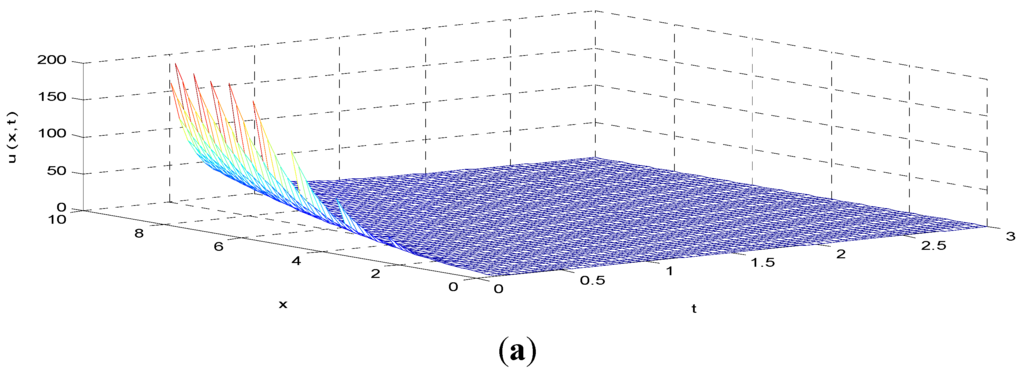
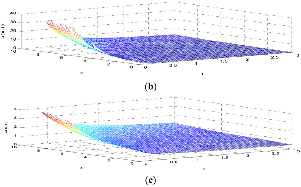
Figure 1.
(a) Exact solution Equation (18) for α = 2, β = 2, γ = 0.6, and n = 2; (b) Exact solution Equation (18) for α = 2, β = 2, γ = 0.6, and n = 3; (c) Exact solution Equation (18) for α = 2, β = 2, γ = 0.6, and n = 5.
3. The Generalized Burgers’–KdV Equation “GBKdV”
The generalized Burgers’–KdV equation “GBKdV” [12,13] will be studied by using the Lie group method.
Consider the generalized Burgers’–KdV equation in form:
with the initial and boundary conditions
Apply Lie group again to Equation (19) as we did before in Equation (2) with the infinitesimal generator
Since the generalized Burgers’–KdV equation has at most third-order derivatives, we prolong the vector field X in Equation (24) to the third order. The action of Pr(3)X on Equation (19) must vanish, where u is the solution of Equation (19). Clearly, the determining Equations can be split with respect to different powers of u. Special cases of splitting cases arise if n ≠ 2 and if n = 2. Therefore, we investigate two cases, namely n ≠ 2 and n = 2
Case 1: For n ≠ 2, the determining equations are:
We have found all possible forms of g = g(t) when Equation (19) admits different Lie algebras of invariance:
Our initial and boundary conditions are satisfied only for Case 1 in Table 2, so . Then the infinitesimal generator of the symmetry group admitted by Equation (19) is given by , and the action of X on Equation (21) must vanish, i.e.,
Table 2.
Infinitesimals .
| No. | g | Infinitesimals |
|---|---|---|
| 1 | ,, | |
| 2 | 1 | ,, |
This gives , , and , from which we get:
The auxiliary equation will be:
Solving Equation (28)
By inserting Equation (29) in Equation (19), it will be reduced to an ODE
The conditions reduce to
Equations (30)–(33) are identical with the results obtained by [13] for .
We use the fourth, fifth-order Runge–Kutta method to solve Equation (30).
Solutions of Equation (30) are plotted in Figure 2 with two different values of the nonlinearity index “n” (n = 5 and 100). The figure shows the vibrations of the variable “F” increase with the increase of the nonlinearity index “n” values and the wave length is seen to decrease with increasing values of “η”. The shape of these waves seems to be a bugle or the sound waves are reborn from the bugle, so we can name these waves as “Bugle-shaped waves”.
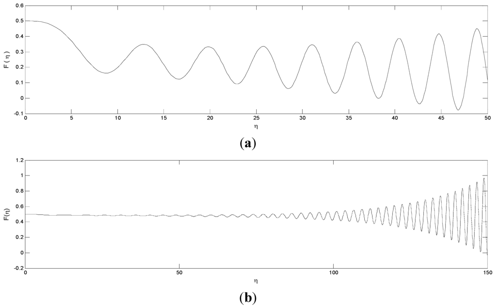
Figure 2.
(a) Bugle-shaped wave solution of BKdV Burgers’–KdV Equation (30) for α = 1, β = 10, and n = 5; (b) Bugle-shaped wave solution of BKdV Burgers’–KdV Equation (30) for α = 1, β = 10, and n = 100.
Case (2): For n = 2, the determining equations are:
We have found all possible forms of g = g(t) when Equation (19) with n = 2 admits different Lie algebras of invariance.
One may note that or from Table 3 also satisfy our initial and boundary conditions, and we can repeat the same procedure from Equation (26) to Equation (33).
This case is completely new and has not been considered before by Abd-el-Malek and Helal [13].
Table 3.
Infinitesimals .
| No. | g | Infinitesimals |
|---|---|---|
| 1 | , , | |
| 2 | , , | |
| 3 | 1 | , , |
| 4 | , , |
4. The Generalized KdV Equation “GKdV”
We introduce the following generalized KdV (GKdV) equation [13,21],
with initial and boundary conditions
This type of GKdV equation with variable coefficients has several important physical circumstances such as coastal waves in oceans, liquid drops and bubbles, and most interestingly, the atmospheric blocking phenomenon, particularly dipole blocking [22]. The first term of Equation (35) is the evolution term, the second term represents the nonlinear term, the third term is the linear damping with time-dependent coefficient w(t), and the fourth term is the dispersion term with time-dependent coefficient g(t).
The term w(t)u in the generalized KdV Equation (35) can be removed by the point transformation as in [23,24]:
By substituting Equation (40) in Equation (35) we get:
All results in Lie symmetries and exact solutions for Equation (35) can be derived from similar results obtained for Equation (41).
Apply Lie group again on Equation (41) as we did before in Equation (19) with the infinitesimal generator
Since the generalized KdV equation has at most third-order derivatives, we prolong the vector field X in Equation (42) to the third order. The action of Pr(3)X on Equation (41) vanishes where ν, the solution of Equation (41), is, and then we find the following determining equations:
The general solution of Equation (43) is
with the following restriction .
We have found all possible forms of when Equation (41) admits different Lie algebras of invariance.
Clearly, by substituting in Equation (35), the latter reduces to Equation (41) with the same initial and boundary conditions in Equations (36)–(39) (i.e., u = ν). The same result is also obtained by substituting w(t) = 0 in Equation (40).
It can be easily checked using Equation (40) that when , both and are power functions.
By substituting in Equation (35), we get:
with initial and boundary conditions in Equations (36)–(39).
By substituting in Equation (40) and by using Case 2 in Table 4, Equation (45) reduces to
which admits the Lie symmetry generators
The action of X on Equation (37) must vanish, i.e.,
This gives
Table 4.
Infinitesimals of .
| No. | Infinitesimals | |
|---|---|---|
| 1 | , , | |
| 2 | ,, | |
| 3 | ,, | |
| 4 | ,, |
We have shown that Equation (45) admits the Lie symmetry generator Equation (47), which keeps the boundary condition invariant if and only if is a power function or constant.
The auxiliary equation is
Solving Equation (50), we get:
From Equations (49) and (51), u(x,t) = by choosing λ(1 − δn) − δn −2 <0. Therefore, and as . Hence, the solution in this case exists; otherwise, a smooth solution of the problem may not exist.
By substituting Equation (51) in Equation (35), we get:
Equation (52) can be written in the form
Assume , and by setting δ = 1, then λ(1 − δn) − δn −2 < 0. Thus, Equation (53) reduces to
Integrating Equation (54) once, we get:
where is a constant. The condition that F(0) = γ leads to , therefore
Equation (56) as well as Equations (57) and (58) are identical with the results obtained by Abd-el-Malek and Helal [13] only for and . We use the fourth, fifth-order Runge–Kutta method to solve Equations (56)–(58).
It is clear that the wave vibrations of F take on a blubber vase-shaped wave as in Figure 3a,d with an increase in the value of “η”. Figure 3b,d display the alternations of the variable F which increases with the increase of the nonlinearity index “n” and the wavelength is seen to decrease with increasing values of “η”.
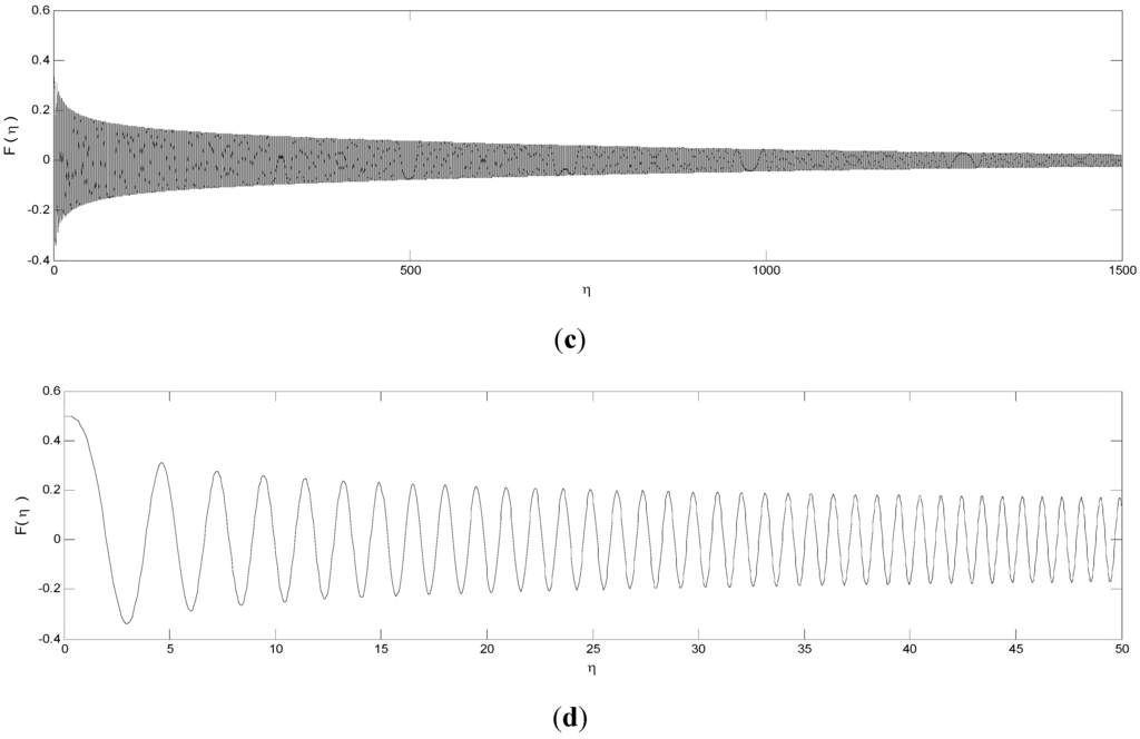
Figure 3.
(a) Wave solution of boundary-value problem (56)–(58) for , , ; (b) Wave solution of boundary-value problem (56)–(58) for , , and ; (c) Wave solution of boundary-value problem (56)–(58) for , n = 100, ; (d) Wave solution of boundary-value problem (56)–(58) for n =100, , and .
We also succeeded to find other possible forms of g(t), but the only case which keeps the boundary conditions invariant is a power function or constant.
5. Concluding Remarks
In this paper, we applied the Lie group method to generate all symmetries for the three nonlinear partial differential equations, namely generalized Burgers’, Burgers’–KdV, and GKdV with initial and boundary conditions. We used the suitable symmetry which satisfies the initial and boundary conditions to reduce the partial differential equations to ordinary differential equations. According to the Lie group method, the traveling wave solutions of all the given equations can be obtained.
Also, the function g(t) in the partial differential equations cannot take exponential form as our initial and boundary condition will not be satisfied. We were able to find more solutions than those that were obtained before by Abd-el-Malek and Helal [13].
The Lie group method can be applied easily to solve boundary value problems by simple procedures.
Finally, in Section 2, we succeeded in constructing the exact solution that describes the velocity field of the generalized Burgers’ equation. However, in Section 3 and Section 4, the reduced ordinary differential equations could not be solved analytically, only numerically. The effect of the nonlinearity index on the solutions was examined and the numerical solutions are graphically presented.
Acknowledgments
The authors would like to express their gratitude to the expert reviewers for their valuable comments that improved the paper to the present form.
Author Contributions
Mina Abd-el-Malek was responsible for suggesting the problem, reviewing the results and editing the writings; Amr Amin was responsible for the calculations and the writing of the manuscript.
Conflicts of Interest
The authors declare no conflict of interest.
References
- Burgers, J.M. A Mathematical Model Illustrating the Theory of Turbulence; Academic Press: New York, NY, USA, 1948. [Google Scholar]
- Su, N.; Watt, J.P.C.; Vincent, K.W.; Close, M.E.; Mao, R. Analysis of Turbulent Flow Patterns of Soil Water under Field Conditions Using Burgers’ Equation and Porous Suction—Cup Samplers. Aust. J. Soil Res. 2004, 42, 9–16. [Google Scholar] [CrossRef]
- Turitsyn, S.; Aceves, A.; Jones, C.K.R.T.; Zharnitsky, V. Average dynamics of the optical soliton in communication lines with dispersion management, analytical results. Phys. Rev. E 1998, 58, R48–R51. [Google Scholar] [CrossRef]
- Cole, J.D. On a quasi linear parabolic Equation occurring in aerodynamics. Quart. Appl. Math. 1951, 9, 225–236. [Google Scholar]
- Hopf, E. The partial differential Equation ut + uux = μuxx. Comm. Pure Appl. Math. 1950, 33, 201–230. [Google Scholar]
- Jeffrey, A.; Mohamad, M.N.B. Exact solutions to the KdV–Burgers’ Equation. Motion 1991, 14, 369–375. [Google Scholar] [CrossRef]
- Kadalbajoo, M.K.; Awasthi, A. A Numerical Method Based on Crank—Nicolson scheme for Burgers’ Equation. Appl. Math. Comput. 2006, 182, 1430–1442. [Google Scholar] [CrossRef]
- Gorguis, A. A Comparison between Cole–Hopf transformation and decomposition method for solving Burgers’ Equation. Appl. Math. Comput. 2006, 173, 126–136. [Google Scholar] [CrossRef]
- Kutluay, S.; Esen, A.; Dag, I. Numerical solutions of the Burgers’ Equation by the least—Squares quadratic B—Spline finite element method. J. Comput. Appl. Math. 2004, 167, 21–33. [Google Scholar] [CrossRef]
- Ames, W.F.; Nucci, M.C. Analysis of fluid Equations by group method. J. Eng. Math. 1985, 20, 181–187. [Google Scholar] [CrossRef]
- Hammerton, P.W.; Crighton, D.G. Approximate solution methods for nonlinear acoustic propagation over long ranges. Proc. R. Soc. Lond. A 1989, 426, 125–152. [Google Scholar] [CrossRef]
- Wazwaz, A. Travelling wave solutions of generalized forms of Burgers, Burgers–KdV and Burgers–Huxley Equations. Appl. Math. Comput. 2005, 169, 639–656. [Google Scholar] [CrossRef]
- Abd-el-Malek, M.B.; Helal, M.M. Group method solutions of the generalized forms of Burgers, Burgers–KdV and KdV Equations with time -dependent variable coefficients. Acta Mech. 2011, 221, 281–296. [Google Scholar] [CrossRef]
- Bluman, G.W.; Kumei, S. Symmetries and Differential Equations; Springer: Berlin, Germany, 1989. [Google Scholar]
- Bluman, G.W.; Anco, S.C. Symmetry and Integration Methods for Differential Equations; Applied Mathematical Sciences; Springer-Verlag: New York, NY, USA, 2002; Volume 154. [Google Scholar]
- Cherniha, R.; Kovalenko, S. Lie symmetries of nonlinear boundary value problems. Commun. Nonlinear Sci. Numer. Simulat. 2012, 17, 71–84. [Google Scholar] [CrossRef]
- Cherniha, R.; King, J.R. Lie and conditional symmetries of a class of nonlinear (1 + 2) dimensional boundary value problems. Symmetry 2015, 7, 1410–1435. [Google Scholar] [CrossRef]
- Olver, P.J. Applications of Lie Groups to Differential Equations; Springer: Berlin, Germany, 1986. [Google Scholar]
- Ovsiannikov, L.V. Group Analysis of Differential Equations; Academic Press: New York, NY, USA, 1982. [Google Scholar]
- Cherniha, R.; Serov, M. Symmetries, Ansaetze and Exact Solutions of Nonlinear Second-order Evolution Equations with Convection Terms, II. Eur. J. Appl. Math. 2006, 17, 597–605. [Google Scholar] [CrossRef]
- Senthilkumaran, M.; Pandiaraja, D.; Vaganan, B.M. New exact explicit solutions of the generalized KdV Equations. Appl. Math. Comput. 2008, 202, 693–699. [Google Scholar] [CrossRef]
- Tang, X.-Y.; Huang, F.; Lou, S.-Y. Variable coefficient KdV Equation and the analytical diagnoses of a dipole blocking life cycle. Chin. Phys. Lett. 2006, 23, 887–890. [Google Scholar]
- Vaneeva, O.O.; Papanicolaou, N.C.; Christou, M.A.; Sophocleous, C. Numerical solutions of boundary value problems for variable coefficient generalized KdV Equations using Lie symmetries. Commun. Nonlinear Sci. Numer. Simul. 2014, 19, 3074–3085. [Google Scholar] [CrossRef]
- Popovych, R.O.; Vaneeva, O.O. More common errors in finding exact solutions of nonlinear differential Equations: Part I. Commun. Nonlinear Sci. Numer. Simulat. 2010, 15, 3887–3899. [Google Scholar] [CrossRef]
© 2015 by the authors; licensee MDPI, Basel, Switzerland. This article is an open access article distributed under the terms and conditions of the Creative Commons Attribution license (http://creativecommons.org/licenses/by/4.0/).