Symbolic and Iterative Computation of Quasi-Filiform Nilpotent Lie Algebras of Dimension Nine

Abstract

This paper addresses the problem of computing the family of two-filiform Lie algebra laws of dimension nine using three Lie algebra properties converted into matrix form properties: Jacobi identity, nilpotence and quasi-filiform property. The interest in this family is broad, both within the academic community and the industrial engineering community, since nilpotent Lie algebras are applied in traditional mechanical dynamic problems and current scientific disciplines. The conditions of being quasi-filiform and nilpotent are applied carefully and in several stages, and appropriate changes of the basis are achieved in an iterative and interactive process of simplification. This has been implemented by means of the development of more than thirty Maple modules. The process has led from the first family formulation, with 64 parameters and 215 constraints, to a family of 16 parameters and 17 constraints. This structure theorem permits the exhaustive classification of the quasi-filiform nilpotent Lie algebras of dimension nine with current computational methodologies.

1. Introduction

1.1. State of the Art

Traditionally, Lie algebras have been used in physics in the context of symmetry groups of dynamical systems, as a powerful tool to study the underlying conservation laws [1,2]. At present, space-time symmetries and symmetries related to degrees of freedom are considered. For instance, non-trivial Heidelberg algebra arises right in the base of the Hamiltonian mechanics. Hamiltonian mechanics describes the state of a dynamic system with $2n$ variables (n coordinates and n momenta), and the other interesting observable physics quantities are functions of them. Thus, the observables commute with the Hamiltonian respecting the Poisson bracket, and they constitute a Lie algebra of infinite dimension. Furthermore, a description in quantum mechanics is obtained by an algebra of Hermitian operators in a Hilbert space with the bracket product as the commutator. In such a case, the Heisenberg algebra arises if n is one, and the generalized Heisenberg algebra results for other values of n, since the traditional canonical variables preserve the Poisson bracket. In general, a transformation is said to be symplectic if it preserves the Poisson bracket. Therefore, the study of symplectic structures of nilpotent Lie algebras is worthwhile as a wide generalization of the Heisenberg algebra. These symplectic Lie algebras appear in the study of traditional dynamic problems, like the problem of the two bodies or the problem of the three bodies, as well as in current studies in solid state physics [3], modern geometry [4] or particle physics [5]. Furthermore, Lie theory is closely connected to control theory in the controllability and optimization of the tracking without drift of complex dynamical systems as a rolling sphere. Some other applications can be consulted in [6,7,8]. Hence, it is convenient to classify the families of Lie algebras as large as possible.

The matter of Lie algebra classification comes down to classifying the solvable semisimple algebras [9,10,11], since Levi’s decomposition theorem [12] permits one to state that any Lie algebra can be decomposed into a semidirect sum of its radical, i.e., its maximal solvable ideal, and a semisimple part called Levi’s subalgebra. The classification of semisimple Lie algebras in $\mathbf{C}$ is presently associated with Dynkin diagrams (1945). However, the solvable Lie algebra classification problem comes down in a sense (Goze and Khakimdjanov [12]) to the nilpotent Lie algebra classification.

Numerous researchers have tackled the problem of nilpotent Lie algebra classification. However, their studies were restricted to the filiform case, due to the difficulties arising from a nilpotence index higher than the dimension, providing a great number of parameters without restrictions among them. The first lists of algebras were obtained by K. Umlauf [13] in 1891 in his PhD thesis, providing the lists of all of the laws of dimensions less than or equal to six and all of dimensions 7, 8 and 9 that allow a basis $\left\{X_0,X_1,...,X_{n-1}\right\}$, such that it satisfies $\left[X_0,X_i\right]=X_{i+1}$ $\left(1⩽i⩽n-2\right)$, in $\mathbf{R}$ or $\mathbf{C}$. Nilpotent Lie algebra classification had important progress thanks to Goze and Ancochea [14] with the definition of a more powerful invariant than the known invariants up to that moment: the characteristic series or Goze’s invariant. These authors achieved the classification of the complex nilpotent Lie algebras of dimension seven and of the complex filiform Lie algebras of dimension eight [15]. Gómez and Echarte [16] classified the complex filiform Lie algebras of dimension nine using Goze’s invariant. Gómez et al. [17] classified the symplectic filiform Lie algebras that are not two-to-two symplectic-isomorphic of dimensions less than or equal to 10 in 2001. Higher dimensions were tackled by Boza et al. [18] and Echarte et al. [19,20] in the last ten years. The more the dimension increases, the more and more complex is the determination of exhaustive lists of Lie algebras, so new computation methodologies are a present field of research [21,22,23].

Cabezas et al. (1998) [24] study a family of Lie algebras that they call p-filiform with dimension n and Goze’s invariant $\left(n-p,1,...,1\right).$ Since filiform algebras have Goze’s invariant $\left(n-1,1\right)$, they are included in the p-filiform family as one-filiform Lie algebras; analogously, the quasi-filiform algebras are the two-filiform algebras [25], and the abelian algebras are the $\left(n-1\right)$-filiform algebras. In a sense, the study of the quasi-filiform Lie algebras appears natural, since they are only known until dimension eight. On the other hand, in 1999, Camacho [26] studied the $(n-5)$-filiform and $(n-6)$-filiform Lie algebras, closing the classification of the p-filiform Lie algebras up to dimension eight. Another classification of the $(n-5)$-filiform Lie algebras is provided by Ancochea and Campoamor [27]. Their research line is used as the context for our piece of research, leaning on the current availability of symbolic manipulation programs, such as Maple, which allow the user to perform the tedious algebra and routine computations [28,29,30]. The present paper tackles the proof of the structure theorem of quasi-filiform Lie algebras of dimension nine. The classification and a complete casuistry of that family of Lie algebras was published in [31], based on the results of [32]. We strongly recommend the reading of [33,34,35,36,37] to become familiar with Lie algebra terminology and concepts.

After this state of the art, Subsection 1.2. is included to declare the terminology that has been developed from the 1990s to the present. Section 2 is devoted to the symbolic and iterative computational proof of the structure theorem of the laws of every complex quasi-filiform Lie algebra of dimension nine, which is the original contribution of the present paper. Finally, Section 3 summarizes the computational work developed for the appropriate changes of the basis to demonstrate the general theorem.

1.2. Terminology

The abelian algebra of dimension n is the only one with Goze’s invariant $\left(1,...,1\right)$; in metabelian algebras, the characteristic series is $\left(2,...2,1,...1\right)$; in Heisenberg algebras, it is $\left(2,1,...,1\right)$; in filiform algebras, it is $\left(n-1,1\right)$; and in quasi-filiform algebras, it is $\left(n-2,1,1\right)$. From now on, let us use the term $\mathbf{Jac}\left(x,y,z\right)$ for the Jacobi identity: $\mathbf{Jac}\left(x,y,z\right)\iff \mu (x,\mu (y,z))+\mu (y,\mu (z,x))+\mu (z,\mu (x,y))=0$. Additionally, let us use ${\mathcal{B}}^2\left({\mathbf{C}}^{\mathbf{n}}\right)$ for the space of the bilinear applications of ${\mathbf{C}}^{\mathbf{n}}\times {\mathbf{C}}^{\mathbf{n}}$ in ${\mathbf{C}}^{\mathbf{n}}$, and let us choose a basis $\left\{e_0,e_2,...,e_{n-1}\right\}$ of ${\mathbf{C}}^{\mathbf{n}}$. An element α of ${\mathcal{B}}^2$ can be determined from a set of scalars $C_{ij}^k$, called structure constants, defined by $\alpha \left(e_i,e_j\right)=\stackrel{n-1}{\underset{k=0}{\Sigma }}{C}_{ij}^k{e}_k$; thus, ${\mathcal{B}}^2$ can have a structure of affine space. Then, a Lie algebra $\mathfrak{g}$ can be considered as an element of ${\mathcal{B}}^2$; the set ${\mathcal{L}}_n$ of Lie algebras in ${\mathbf{C}}^{\mathbf{n}}$ is the affine algebraic set that is defined by the following polynomial expressions:

$$\begin{array}{ccc}& & C_{ii}^k=0,\forall i,k0⩽i,k⩽n-1\hfill \end{array}$$

(1a)

$$\begin{array}{ccc}& & C_{ij}^k=-C_{ji}^k\forall i,j,k0⩽i,j,k⩽n-1\hfill \end{array}$$

(1b)

$$\begin{array}{ccc}& & \stackrel{n-1}{\underset{k=0}{\Sigma }}\left(C_{ij}^k\text{.}{C}_{kl}^s+C_{jl}^k\text{.}{C}_{ki}^s+C_{li}^k\text{.}{C}_{kj}^s\right)=0,0⩽i,j,l,s⩽n-1\hfill \end{array}$$

(1c)

and it is parametrized by the $\frac{n^3-n^2}{2}$ structure constants $C_{ij}^k$.

If $\mathfrak{g}$ is a Lie algebra, the series of ideals defined by:

$$\begin{array}{ccc}& & {\mathcal{D}}^0\left(\mathfrak{g}\right)=\mathfrak{g}\hfill \end{array}$$

(2a)

$$\begin{array}{ccc}\hfill & & {\mathcal{D}}^{k+1}\left(\mathfrak{g}\right)=\left[{\mathcal{D}}^k\left(\mathfrak{g}\right),{\mathcal{D}}^k\left(\mathfrak{g}\right)\right],k\in \mathbf{N}\cup \left\{0\right\}\hfill \end{array}$$

(2b)

is called the derived series of $\mathfrak{g}$, which satisfies $\mathfrak{g}={\mathcal{D}}^0\left(\mathfrak{g}\right)\supseteq {\mathcal{D}}^1\left(\mathfrak{g}\right)\supseteq ...\supseteq {\mathcal{D}}^i\left(\mathfrak{g}\right)...$ If there exists an integer k, such that ${\mathcal{D}}^k\left(\mathfrak{g}\right)=\left\{0\right\}$, the algebra is said to be solvable; in such a case, the smaller integer that satisfies the previous condition is called the solvability index of $\mathfrak{g}$.

Levi’s theorem [33] states that every Lie algebra $\mathfrak{g}$ can be decomposed in a semidirect sum of its radical (the maximal solvable ideal) and semisimple subalgebras (Levi’s subalgebra). This result reduces in a sense the Lie algebra classification problem to the classification of the solvable algebras [10, since semisimple algebra classification is known.

If $\mathfrak{g}$ is a Lie algebra, the series of ideals defined by:

$$\begin{array}{ccc}& & {\mathcal{C}}^0\left(\mathfrak{g}\right)=\mathfrak{g}\hfill \end{array}$$

(3a)

$$\begin{array}{ccc}& & {\mathcal{C}}^{k+1}\left(\mathfrak{g}\right)=\left[{\mathcal{C}}^k\left(\mathfrak{g}\right),\mathfrak{g}\right],k\in \mathbf{N}\cup \left\{0\right\}\hfill \end{array}$$

(3b)

is called the lower central series of $\mathfrak{g}$. It satisfies that $\mathfrak{g}={\mathcal{C}}^0\left(\mathfrak{g}\right)\supseteq {\mathcal{C}}^1\left(\mathfrak{g}\right)\supseteq ...\supseteq {\mathcal{C}}^i\left(\mathfrak{g}\right)...$ If there exists an integer k, such that ${\mathcal{C}}^k\left(\mathfrak{g}\right)=\left\{0\right\}$, the algebra is said to be nilpotent; in such a case, the smaller integer that satisfies the previous condition is called the nilpotence index or nilindex of $\mathfrak{g}$. If the dimension is n and the nilindex is $n-1$, the algebras obtained are called filiform; they are said to be quasi-filiform if their nilindex is $n-2$. The abelian Lie algebras are the algebras with nilindex one.

The characteristic series or Goze’s invariant is defined as the maximum of the Segre symbols of the nilpotent linear applications $ad\left(X\right)$, where X is an element of the derived subalgebra complementary. In other words, if $\mathfrak{g}$ is a complex nilpotent Lie algebra of finite dimension n, for every $X\in \mathfrak{g}-\left[\mathfrak{g},\mathfrak{g}\right]$, the series of the characteristic subspace dimensions of the nilpotent operator $ad\left(X\right)$ in decreasing order is denoted by $c\left(X\right)=\left(c_1\left(X\right),c_2\left(X\right),,...,1\right).$ Reordering the set of series in lexicographical order, the characteristic series is defined by $c\left(\mathfrak{g}\right)=$ sup$\left\{c\left(X\right):X\in \mathfrak{g}-\left[\mathfrak{g},\mathfrak{g}\right]\right\}.$ This invariant has been used to classify the nilpotent Lie algebras of dimension seven. Obviously, $c\left(\mathfrak{g}\right)$ is an invariant for the isomorphisms, and by construction, there exists at least a vector $X\in \mathfrak{g}-\left[\mathfrak{g},\mathfrak{g}\right]$ that satisfies $c\left(\mathfrak{g}\right)=c\left(X\right)$; every vector that satisfies the previous condition is called the characteristic vector of the algebra.

If $\mathfrak{g}$ is a p-filiform Lie algebra of dimension n (i.e., nilpotent with characteristic series $\left(n-p,1,...,1\right)$, then there exists a basis, which will be denoted as $\left\{X_0,X_1,...,X_p,Y_1,...,Y_{n-p-1}\right\}$, that satisfies:

$$\begin{array}{ccc}& & \left[X_0,X_i\right]=X_{i+1}1⩽i⩽p-1\hfill \end{array}$$

(4a)

$$\begin{array}{ccc}& & \left[X_0,X_{n-p}\right]=0\hfill \end{array}$$

(4b)

$$\begin{array}{ccc}& & \left[X_0,Y_j\right]=01⩽j⩽n-p-1\hfill \end{array}$$

(4c)

This basis is called the adapted basis of the algebra, where $X_0$ is a characteristic vector.

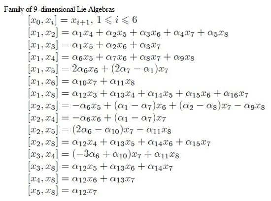
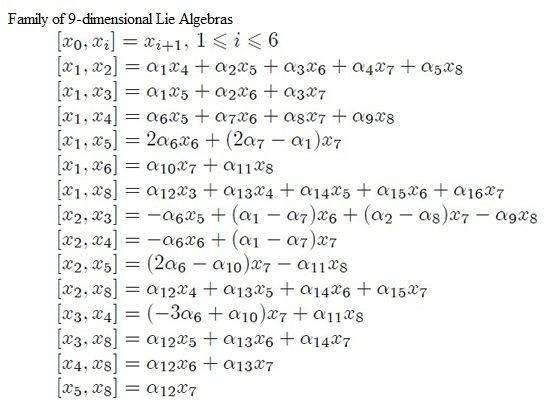
2. Structure Theorem

This section presents the development of the structure theorem of the family of laws of complex quasi-filiform Lie algebras (QFLA) of dimension nine. Our objective was to find the simplest expression of the family of laws. Every QFLA of dimension nine can have an adapted basis $\left\{x_0,x_1,...,x_8\right\}$, such that:

$$\left[x_0,x_i\right]=x_{i+1},1⩽i⩽6;\left[x_0,x_i\right]=0,7⩽i⩽8$$

(5)

A first approximation of the family can be obtained just with the application of the Jacobi identity to the three-tuple ($x_0,x_i,x_j)$, where $x_i,x_j$ are basis vectors different from $x_0$ vector [31].

A condition that sometimes is more difficult to apply is the nilpotence. The Engel theorem puts nilpotence on a level with ad-nilpotence for Lie algebras. Therefore, a Lie algebra $\mathfrak{g}$ is nilpotent if and only if the characteristic polynomial of the matrix $Adj\left(x\right)$ is ${\lambda }^9$, for every vector x of $\mathfrak{g}$. Anyway, this condition is often difficult to apply, so the moment in the process when the nilpotence condition is applied or, much better, when the condition is applied for each vector has to be chosen carefully.

The condition of being quasi-filiform can be also interpreted in terms of matrices. Thus, the vector candidate of characteristic vectors, i.e., the vectors in $\mathfrak{g}-\left[\mathfrak{g},\mathfrak{g}\right]$, has to satisfy that the respective adjoint matrices do not have non-null minors of order $⩽7$. As in the case of the nilpotence, this condition has to be applied with caution and probably in several stages.

Theorem 1. The laws of every complex quasi-filiform Lie algebra of dimension nine can be described by the following family with 16 parameters and 17 polynomial restriction equations:

$$\begin{array}{ccc}& [x_0,x_i]=& x_{i+1},1⩽i⩽6\hfill \end{array}$$

(6a)

$$\begin{array}{ccc}& [x_1,x_2]=& {\alpha }_1{x}_4+{\alpha }_2{x}_5+{\alpha }_3{x}_6+{\alpha }_4{x}_7+{\alpha }_5{x}_8\hfill \end{array}$$

(6b)

$$\begin{array}{ccc}& [x_1,x_3]=& {\alpha }_1{x}_5+{\alpha }_2{x}_6+{\alpha }_3{x}_7\hfill \end{array}$$

(6c)

$$\begin{array}{ccc}& [x_1,x_4]=& {\alpha }_6{x}_5+{\alpha }_7{x}_6+{\alpha }_8{x}_7+{\alpha }_9{x}_8\hfill \end{array}$$

(6d)

$$\begin{array}{ccc}& [x_1,x_5]=& 2{\alpha }_6{x}_6+(2{\alpha }_7-{\alpha }_1)x_7\hfill \end{array}$$

(6e)

$$\begin{array}{ccc}& [x_1,x_6]=& {\alpha }_{10}{x}_7+{\alpha }_{11}{x}_8\hfill \end{array}$$

(6f)

$$\begin{array}{ccc}& [x_1,x_8]=& {\alpha }_{12}{x}_3+{\alpha }_{13}{x}_4+{\alpha }_{14}{x}_5+{\alpha }_{15}{x}_6+{\alpha }_{16}{x}_7\hfill \end{array}$$

(6g)

$$\begin{array}{ccc}& [x_2,x_3]=& -{\alpha }_6{x}_5+({\alpha }_1-{\alpha }_7)x_6+({\alpha }_2-{\alpha }_8)x_7-{\alpha }_9{x}_8\hfill \end{array}$$

(6h)

$$\begin{array}{ccc}& [x_2,x_4]=& -{\alpha }_6{x}_6+({\alpha }_1-{\alpha }_7)x_7\hfill \end{array}$$

(6i)

$$\begin{array}{ccc}& [x_2,x_5]=& (2{\alpha }_6-{\alpha }_{10})x_7-{\alpha }_{11}{x}_8\hfill \end{array}$$

(6j)

$$\begin{array}{ccc}& [x_2,x_8]=& {\alpha }_{12}{x}_4+{\alpha }_{13}{x}_5+{\alpha }_{14}{x}_6+{\alpha }_{15}{x}_7\hfill \end{array}$$

(6k)

$$\begin{array}{ccc}& [x_3,x_4]=& (-3{\alpha }_6+{\alpha }_{10})x_7+{\alpha }_{11}{x}_8\hfill \end{array}$$

(6l)

$$\begin{array}{ccc}& [x_3,x_8]=& {\alpha }_{12}{x}_5+{\alpha }_{13}{x}_6+{\alpha }_{14}{x}_7\hfill \end{array}$$

(6m)

$$\begin{array}{ccc}& [x_4,x_8]=& {\alpha }_{12}{x}_6+{\alpha }_{13}{x}_7\hfill \end{array}$$

(6n)

$$\begin{array}{ccc}& [x_5,x_8]=& {\alpha }_{12}{x}_7\hfill \end{array}$$

(6o)

subject to:

$$\begin{array}{ccc}\hfill & & {\alpha }_5{\alpha }_{12}=0\hfill \end{array}$$

(7a)

$$\begin{array}{ccc}& & {\alpha }_6{\alpha }_{12}=0\hfill \end{array}$$

(7b)

$$\begin{array}{ccc}& & {\alpha }_6{\alpha }_{13}=0\hfill \end{array}$$

(7c)

$$\begin{array}{ccc}& & {\alpha }_9{\alpha }_{12}=0\hfill \end{array}$$

(7d)

$$\begin{array}{ccc}& & {\alpha }_9{\alpha }_{13}=0\hfill \end{array}$$

(7e)

$$\begin{array}{ccc}& & {\alpha }_9{\alpha }_{14}=0\hfill \end{array}$$

(7f)

$$\begin{array}{ccc}& & {\alpha }_{10}{\alpha }_{12}=0\hfill \end{array}$$

(7g)

$$\begin{array}{ccc}& & {\alpha }_{11}{\alpha }_{12}=0\hfill \end{array}$$

(7h)

$$\begin{array}{ccc}& & {\alpha }_{11}{\alpha }_{13}=0\hfill \end{array}$$

(7i)

$$\begin{array}{ccc}& & {\alpha }_{11}{\alpha }_{14}=0\hfill \end{array}$$

(7j)

$$\begin{array}{ccc}& & {\alpha }_{11}{\alpha }_{15}=0\hfill \end{array}$$

(7k)

$$\begin{array}{ccc}& & {\alpha }_{11}{\alpha }_{16}=0\hfill \end{array}$$

(7l)

$$\begin{array}{ccc}& & {\alpha }_{11}\left(3{\alpha }_1-{\alpha }_7\right)=0\hfill \end{array}$$

(7m)

$$\begin{array}{ccc}& & {\alpha }_{12}\left({\alpha }_1-{\alpha }_7\right)=0\hfill \end{array}$$

(7n)

$$\begin{array}{ccc}& & {\alpha }_5{\alpha }_{13}-2{\alpha }_6^2-{\alpha }_9{\alpha }_{15}\hfill \end{array}$$

(7o)

$$\begin{array}{ccc}& & 2({\alpha }_2-{\alpha }_8){\alpha }_{12}+3({\alpha }_1-{\alpha }_7){\alpha }_{13}+2({\alpha }_6-{\alpha }_{10}){\alpha }_{14}=0\hfill \end{array}$$

(7p)

$$\begin{array}{ccc}& & {\alpha }_5{\alpha }_{14}-2(2{\alpha }_1+{\alpha }_7){\alpha }_6-{\alpha }_9{\alpha }_{16}+(3{\alpha }_1-{\alpha }_7){\alpha }_{10}=0\hfill \end{array}$$

(7q)

Proof of Theorem 1. Let $\mathfrak{g}$ be a nilpotent Lie algebra of dimension n and the characteristic series ($n-2,1,1$). Let $x_0\in \mathfrak{g}-\left[\mathfrak{g},\mathfrak{g}\right]$ be a characteristic vector of $\mathfrak{g}$. Then, there is a basis of $\mathfrak{g}$, $\left\{x_i:0⩽i⩽n-1\right\}$, such that $\left[x_0,x_i\right]=x_{i+1}$, $1⩽i⩽n-3$, and the other bracket products of $x_0$ are null. On the whole, all of the bracket products can be described by:

$$\left[x_i,x_j\right]=\stackrel{n-1}{\underset{k=0}{\Sigma }}{C}_{ij}^k.x_k,0⩽i,j⩽n-1$$

(8)

where $C_{ij}^k$ are the algebra structure constants. It is simple to prove that for a nilpotent Lie algebra of dimension n and characteristic series $\left(n-2,1,1..,1\right)$, like ${\mathcal{C}}^m\mathfrak{g}=$ $〈x_{n-2}〉$, it is true that $x_{n-2}\in \mathit{Z}\left(\mathfrak{g}\right)$. Then, in our case:

$$\left[x_{n-2},x_j\right]=0,\forall j0⩽j⩽n-1\to C_{(n-2)j}^k=0,\forall j,k0⩽j,k⩽n-1$$

(9)

It is well known that the application of the anticommutativity to Jacobi identity will provide $\mathbf{Jac}(y,x,z)\equiv \left[x,\left[y,z\right]\right]=\left[y,\left[x,z\right]\right]-\left[z,\left[x,y\right]\right].$ In order to maintain this identity, the coefficients of $x_i$, $0⩽i⩽n-1$, must be the same at both sides of the equation. Our objective is to study the case $n=9$; therefore, the coefficients’ identification is tackled in an iterative and interactive way. A Maple module called EcuJac has been developed to obtain all of the equations resulting from the application of the aforementioned conditions. Figure 1 illustrates how the Maple module for applying the Jacobi identity conditions has been written. EcuJac is executed iteratively, and each time, it prints a number of equations, so that the number of equations can be reduced in the next iteration. The other proprietary modules executed in EcuJac (Leyes, ObtEcus, OrdApIIG and SimplEcu) are not provided, but their functionalities are commented on in Figure 1.

Figure 1. Module for the application of the Jacobi identity conditions.

Figure 1. Module for the application of the Jacobi identity conditions.

Before each new iteration of EcuJac, the simplest conditions are applied, and the process is repeated until there are no restrictions of simple application. Thus, after a first iteration of module EcuJac with substitutions like:

$$\begin{array}{cc}& \text{From}{Jac(x}_0{,x}_6{,x}_8)\to C_{68}^1{=C}_{68}^2{=C}_{68}^3{=C}_{68}^4{=C}_{68}^5{=C}_{68}^6=0\hfill \end{array}$$

(10a)

$$\begin{array}{cc}& \text{From}{Jac(x}_0{,x}_5{,x}_8)\to \hfill \end{array}$$

$$\begin{array}{cc}& C_{58}^1{=C}_{58}^2{=C}_{58}^3{=C}_{58}^4{=C}_{58}^5{=C}_{68}^8{=0,C}_{68}^7{=C}_{58}^6\hfill \end{array}$$

(10b)

$$\begin{array}{cc}& \text{From}{Jac(x}_0{,x}_4{,x}_8)\to \hfill \end{array}$$

$$\begin{array}{cc}& C_{48}^1{=C}_{48}^2{=C}_{48}^3{=C}_{48}^4{=C}_{58}^8{=0,C}_{58}^6{=C}_{48}^5{,C}_{58}^7{=C}_{48}^6\hfill \end{array}$$

(10c)

215 equations are obtained; some of them are repeated, and others are identities. Selecting one of the simplest equations, like the one that corresponds to the coefficient of $x_6$ in $\mathbf{Jac}(x_0,x_3,x_5)\to C_{35}^5-C_{45}^6-C_{36}^6=0$, it is possible to achieve the subsequent substitutions, like $C_{45}^5=C_{16}^3$, $C_{45}^6=C_{16}^4$, and to compute again the Jacobi equations (EcuJac), obtaining 151 equations. Subsequent iterations provide 124 equations, 78 equations and 55 equations. Then, the first description of the laws is:

$$\begin{array}{cc}& [x_0,x_i]=x_{i+1},1⩽i⩽6\hfill \end{array}$$

(11a)

$$\begin{array}{cc}& [x_1,x_2]=C_{12}^1{x}_1+C_{12}^2{x}_2+C_{12}^3{x}_3+C_{12}^4{x}_4+C_{12}^5{x}_5\hfill \end{array}$$

$$\begin{array}{cc}& +C_{12}^6{x}_6+C_{12}^7{x}_7+C_{12}^8{x}_8\hfill \end{array}$$

(11b)

$$\begin{array}{cc}& [x_1,x_3]=C_{12}^1{x}_2+C_{12}^2{x}_3+C_{12}^3{x}_4+C_{12}^4{x}_5+C_{12}^5{x}_6+C_{12}^6{x}_7\hfill \end{array}$$

(11c)

$$\begin{array}{cc}& [x_1,x_4]=C_{14}^3{x}_3+C_{14}^4{x}_4+C_{14}^5{x}_5+C_{14}^6{x}_6+C_{14}^7{x}_7+C_{14}^8{x}_8\hfill \end{array}$$

(11d)

$$\begin{array}{cc}& [x_1,x_5]=(2C_{14}^3-C_{12}^1)x_4+(2C_{14}^4-C_{12}^2)x_5\hfill \end{array}$$

$$\begin{array}{cc}& +(2C_{14}^5-C_{12}^3)x_6+(2C_{14}^6-C_{12}^4)x_7\hfill \end{array}$$

(11e)

$$\begin{array}{cc}& [x_1,x_6]=(\frac{5}{3}{C}_{14}^3-C_{12}^1)x_5+(\frac{5}{3}{C}_{14}^4-C_{12}^2)x_6+C_{16}^7{x}_7+C_{16}^8{x}_8\hfill \end{array}$$

(11f)

$$\begin{array}{cc}& [x_1,x_8]=C_{18}^2{x}_2+C_{18}^3{x}_3+C_{18}^4{x}_4+C_{18}^5{x}_5\hfill \end{array}$$

$$\begin{array}{cc}& +C_{18}^6{x}_6+C_{18}^7{x}_7+C_{18}^8{x}_8\hfill \end{array}$$

(11g)

$$\begin{array}{cc}& [x_2,x_3]=(C_{12}^1-C_{14}^3)x_3+(C_{12}^2-C_{14}^4)x_4+(C_{12}^3-C_{14}^5)x_5\hfill \end{array}$$

$$\begin{array}{cc}& +(C_{12}^4-C_{14}^6)x_6+(C_{12}^5-C_{14}^7)-C_{14}^8{x}_8\hfill \end{array}$$

(11h)

$$\begin{array}{cc}& [x_2,x_4]=(C_{12}^1-C_{14}^3)x_4+(C_{12}^2-C_{14}^4)x_5+(C_{12}^3-C_{14}^5)x_6+(C_{12}^4-C_{14}^6)x_7\hfill \end{array}$$

(11i)

$$\begin{array}{cc}& [x_2,x_5]=\frac{1}{3}{C}_{14}^3{x}_5+\frac{1}{3}{C}_{14}^4{x}_6+(2C_{14}^5-C_{12}^3-C_{16}^7)x_7-C_{16}^8{x}_8\hfill \end{array}$$

(11j)

$$\begin{array}{cc}& [x_2,x_6]=(\frac{5}{3}{C}_{14}^3-C_{12}^1)x_6+(\frac{5}{3}{C}_{14}^4-C_{12}^2)x_7\hfill \end{array}$$

(11k)

$$\begin{array}{cc}& [x_2,x_8]=C_{18}^2{x}_3+C_{18}^3{x}_4+C_{18}^4{x}_5+C_{18}^5{x}_6+C_{18}^6{x}_7\hfill \end{array}$$

(11l)

$$\begin{array}{cc}& [x_3,x_4]=(C_{12}^1-\frac{4}{3}{C}_{14}^3)x_5+(C_{12}^2-\frac{4}{3}{C}_{14}^4)x_6+(2C_{12}^3-3C_{14}^5+C_{16}^7)x_7+C_{16}^8{x}_8\hfill \end{array}$$

(11m)

$$\begin{array}{cc}& [x_3,x_5]=(C_{12}^1-\frac{4}{3}{C}_{14}^3)x_6+(C_{12}^2-\frac{4}{3}{C}_{14}^4)x_7\hfill \end{array}$$

(11n)

$$\begin{array}{cc}& [x_3,x_6]=(\frac{5}{3}{C}_{14}^3-C_{12}^1)x_7\hfill \end{array}$$

(11o)

$$\begin{array}{cc}& [x_3,x_8]=C_{18}^2{x}_4+C_{18}^3{x}_5+C_{18}^4{x}_6+C_{18}^5{x}_7\hfill \end{array}$$

(11p)

$$\begin{array}{cc}& [x_4,x_5]=(2C_{12}^1-3C_{14}^3)x_7\hfill \end{array}$$

(11q)

$$\begin{array}{cc}& [x_4,x_8]=C_{18}^2{x}_5+C_{18}^3{x}_6+C_{18}^4{x}_7\hfill \end{array}$$

(11r)

$$\begin{array}{cc}& [x_5,x_8]=C_{18}^2{x}_6+C_{18}^3{x}_7\hfill \end{array}$$

(11s)

$$\begin{array}{cc}& [x_6,x_8]=C_{18}^2{x}_7\hfill \end{array}$$

(11t)

Subject to the restrictions detailed in Table 1 and Table 2.

Table 1. First group of constraints.

(1)	$C_{18}^2{C}_{18}^8=0$
(2)	$-\frac{10}{3}{C}_{14}^3{C}_{18}^3+2C_{18}^3{C}_{12}^1-C_{18}^2{C}_{18}^8=0$
(3)	$-5C_{18}^4{C}_{14}^3+3C_{18}^4{C}_{12}^1-\frac{10}{3}{C}_{18}^3{C}_{14}^4+2C_{18}^3{C}_{12}^2-C_{18}^3{C}_{18}^8=0$
(4)	$-\frac{2}{3}{C}_{18}^3{C}_{14}^3-C_{18}^2{C}_{18}^8=0$
(5)	$-\frac{2}{3}{C}_{18}^3{C}_{14}^4-C_{18}^4{C}_{14}^3-C_{18}^3{C}_{18}^8=0$
(6)	$2C_{16}^7{C}_{18}^3+2C_{18}^5{C}_{14}^3-C_{18}^4{C}_{14}^4-4C_{18}^3{C}_{14}^5+2C_{18}^3{C}_{12}^3-2C_{18}^5{C}_{12}^1-C_{18}^4{C}_{18}^8=0$
(7)	$2C_{16}^8{C}_{18}^3=0$
(8)	$2C_{18}^3{C}_{14}^3-2C_{18}^3{C}_{12}^1-C_{18}^2{C}_{18}^8=0$
(9)	$2C_{18}^3{C}_{14}^4-2C_{18}^3{C}_{12}^2-3C_{18}^4{C}_{12}^1+3C_{18}^4{C}_{14}^3-C_{18}^3{C}_{18}^8=0$
(10)	$2C_{18}^3{C}_{14}^5-2C_{18}^3{C}_{12}^3+3C_{18}^4{C}_{14}^4-3C_{18}^4{C}_{12}^2-2C_{18}^5{C}_{12}^1+\frac{4}{3}{C}_{18}^5{C}_{14}^3-C_{18}^4{C}_{18}^8=0$
(11)	$2C_{14}^6{C}_{18}^3-2C_{18}^3{C}_{12}^4-2C_{18}^5{C}_{12}^2-3C_{18}^4{C}_{12}^3+3C_{18}^4{C}_{14}^5+\frac{4}{3}{C}_{18}^5{C}_{14}^4-\frac{5}{3}{C}_{18}^6{C}_{14}^3-C_{18}^5{C}_{18}^8=0$
(12)	$2C_{14}^7{C}_{18}^3+3C_{18}^4{C}_{14}^6-3C_{18}^4{C}_{12}^4+2C_{16}^7{C}_{18}^5-C_{18}^7{C}_{12}^1-2C_{18}^3{C}_{12}^5-2C_{18}^5{C}_{14}^5-\frac{5}{3}{C}_{18}^6{C}_{14}^4-C_{18}^6{C}_{18}^8=0$
(13)	$2C_{14}^8{C}_{18}^3+2C_{16}^8{C}_{18}^5-C_{18}^8{C}_{12}^1=0$
(14)	$C_{16}^8{C}_{18}^2=0$
(15)	$C_{16}^8{C}_{18}^3=0$
(16)	$-\frac{10}{3}{\left(C_{14}^3\right)}^2+\frac{16}{3}{C}_{14}^3{C}_{12}^1-C_{14}^8{C}_{18}^2-2{\left(C_{12}^1\right)}^2+C_{16}^8{C}_{18}^4=0$
(17)	$\frac{14}{3}{C}_{14}^3{C}_{12}^1-2{\left(C_{12}^1\right)}^2-\frac{20}{9}{\left(C_{14}^3\right)}^2+C_{16}^8{C}_{18}^4=0$
(18)	$\frac{4}{3}{C}_{14}^4{C}_{12}^1-2C_{12}^2{C}_{12}^1+\frac{5}{3}{C}_{14}^3{C}_{12}^2+\frac{5}{9}{C}_{14}^3{C}_{14}^4+C_{16}^8{C}_{18}^5=0$
(19)	$\frac{20}{9}{\left(C_{14}^3\right)}^2-\frac{14}{3}{C}_{14}^3{C}_{12}^1+2{\left(C_{12}^1\right)}^2-C_{16}^8{C}_{18}^4=0$
(20)	$-\frac{4}{3}{C}_{14}^4{C}_{12}^1+2C_{12}^2{C}_{12}^1-\frac{5}{3}{C}_{14}^3{C}_{12}^2-\frac{5}{9}{C}_{14}^3{C}_{14}^4-C_{16}^8{C}_{18}^5=0$
(21)	$\frac{10}{3}{C}_{16}^7{C}_{14}^3-3C_{16}^7{C}_{12}^1+\frac{5}{3}{C}_{12}^2{C}_{14}^4+C_{18}^2{C}_{12}^8-\frac{10}{3}{C}_{14}^5{C}_{14}^3+2C_{14}^5{C}_{12}^1-\frac{25}{9}{\left(C_{14}^4\right)}^2-C_{18}^6{C}_{16}^8=0$
(22)	$C_{14}^3{C}_{12}^1-\frac{4}{3}{\left(C_{14}^3\right)}^2-C_{14}^8{C}_{18}^2=0$
(23)	$4C_{14}^3{C}_{12}^2-\frac{31}{3}{C}_{14}^3{C}_{14}^4+6C_{14}^4{C}_{12}^1-C_{14}^8{C}_{18}^3-2C_{12}^2{C}_{12}^1=0$
(24)	$-\frac{2}{3}{C}_{14}^3{C}_{12}^1+\frac{4}{9}{\left(C_{14}^3\right)}^2=0$
(25)	$-2C_{14}^4{C}_{12}^1+\frac{28}{9}{C}_{14}^3{C}_{14}^4-\frac{2}{3}{C}_{14}^3{C}_{12}^2=0$
(26)	$3C_{16}^7{C}_{12}^1-\frac{10}{3}{C}_{16}^7{C}_{14}^3-3C_{14}^5{C}_{12}^1-2C_{12}^2{C}_{14}^4+\frac{2}{3}{C}_{12}^3{C}_{14}^3+\frac{8}{3}{C}_{14}^5{C}_{14}^3+\frac{8}{3}{\left(C_{14}^4\right)}^2=0$
(27)	$3C_{16}^8{C}_{12}^1-\frac{10}{3}{C}_{16}^8{C}_{14}^3=0$

Table 1. First group of constraints.

(1)	$C_{18}^2{C}_{18}^8=0$
(2)	$-\frac{10}{3}{C}_{14}^3{C}_{18}^3+2C_{18}^3{C}_{12}^1-C_{18}^2{C}_{18}^8=0$
(3)	$-5C_{18}^4{C}_{14}^3+3C_{18}^4{C}_{12}^1-\frac{10}{3}{C}_{18}^3{C}_{14}^4+2C_{18}^3{C}_{12}^2-C_{18}^3{C}_{18}^8=0$
(4)	$-\frac{2}{3}{C}_{18}^3{C}_{14}^3-C_{18}^2{C}_{18}^8=0$
(5)	$-\frac{2}{3}{C}_{18}^3{C}_{14}^4-C_{18}^4{C}_{14}^3-C_{18}^3{C}_{18}^8=0$
(6)	$2C_{16}^7{C}_{18}^3+2C_{18}^5{C}_{14}^3-C_{18}^4{C}_{14}^4-4C_{18}^3{C}_{14}^5+2C_{18}^3{C}_{12}^3-2C_{18}^5{C}_{12}^1-C_{18}^4{C}_{18}^8=0$
(7)	$2C_{16}^8{C}_{18}^3=0$
(8)	$2C_{18}^3{C}_{14}^3-2C_{18}^3{C}_{12}^1-C_{18}^2{C}_{18}^8=0$
(9)	$2C_{18}^3{C}_{14}^4-2C_{18}^3{C}_{12}^2-3C_{18}^4{C}_{12}^1+3C_{18}^4{C}_{14}^3-C_{18}^3{C}_{18}^8=0$
(10)	$2C_{18}^3{C}_{14}^5-2C_{18}^3{C}_{12}^3+3C_{18}^4{C}_{14}^4-3C_{18}^4{C}_{12}^2-2C_{18}^5{C}_{12}^1+\frac{4}{3}{C}_{18}^5{C}_{14}^3-C_{18}^4{C}_{18}^8=0$
(11)	$2C_{14}^6{C}_{18}^3-2C_{18}^3{C}_{12}^4-2C_{18}^5{C}_{12}^2-3C_{18}^4{C}_{12}^3+3C_{18}^4{C}_{14}^5+\frac{4}{3}{C}_{18}^5{C}_{14}^4-\frac{5}{3}{C}_{18}^6{C}_{14}^3-C_{18}^5{C}_{18}^8=0$
(12)	$2C_{14}^7{C}_{18}^3+3C_{18}^4{C}_{14}^6-3C_{18}^4{C}_{12}^4+2C_{16}^7{C}_{18}^5-C_{18}^7{C}_{12}^1-2C_{18}^3{C}_{12}^5-2C_{18}^5{C}_{14}^5-\frac{5}{3}{C}_{18}^6{C}_{14}^4-C_{18}^6{C}_{18}^8=0$
(13)	$2C_{14}^8{C}_{18}^3+2C_{16}^8{C}_{18}^5-C_{18}^8{C}_{12}^1=0$
(14)	$C_{16}^8{C}_{18}^2=0$
(15)	$C_{16}^8{C}_{18}^3=0$
(16)	$-\frac{10}{3}{\left(C_{14}^3\right)}^2+\frac{16}{3}{C}_{14}^3{C}_{12}^1-C_{14}^8{C}_{18}^2-2{\left(C_{12}^1\right)}^2+C_{16}^8{C}_{18}^4=0$
(17)	$\frac{14}{3}{C}_{14}^3{C}_{12}^1-2{\left(C_{12}^1\right)}^2-\frac{20}{9}{\left(C_{14}^3\right)}^2+C_{16}^8{C}_{18}^4=0$
(18)	$\frac{4}{3}{C}_{14}^4{C}_{12}^1-2C_{12}^2{C}_{12}^1+\frac{5}{3}{C}_{14}^3{C}_{12}^2+\frac{5}{9}{C}_{14}^3{C}_{14}^4+C_{16}^8{C}_{18}^5=0$
(19)	$\frac{20}{9}{\left(C_{14}^3\right)}^2-\frac{14}{3}{C}_{14}^3{C}_{12}^1+2{\left(C_{12}^1\right)}^2-C_{16}^8{C}_{18}^4=0$
(20)	$-\frac{4}{3}{C}_{14}^4{C}_{12}^1+2C_{12}^2{C}_{12}^1-\frac{5}{3}{C}_{14}^3{C}_{12}^2-\frac{5}{9}{C}_{14}^3{C}_{14}^4-C_{16}^8{C}_{18}^5=0$
(21)	$\frac{10}{3}{C}_{16}^7{C}_{14}^3-3C_{16}^7{C}_{12}^1+\frac{5}{3}{C}_{12}^2{C}_{14}^4+C_{18}^2{C}_{12}^8-\frac{10}{3}{C}_{14}^5{C}_{14}^3+2C_{14}^5{C}_{12}^1-\frac{25}{9}{\left(C_{14}^4\right)}^2-C_{18}^6{C}_{16}^8=0$
(22)	$C_{14}^3{C}_{12}^1-\frac{4}{3}{\left(C_{14}^3\right)}^2-C_{14}^8{C}_{18}^2=0$
(23)	$4C_{14}^3{C}_{12}^2-\frac{31}{3}{C}_{14}^3{C}_{14}^4+6C_{14}^4{C}_{12}^1-C_{14}^8{C}_{18}^3-2C_{12}^2{C}_{12}^1=0$
(24)	$-\frac{2}{3}{C}_{14}^3{C}_{12}^1+\frac{4}{9}{\left(C_{14}^3\right)}^2=0$
(25)	$-2C_{14}^4{C}_{12}^1+\frac{28}{9}{C}_{14}^3{C}_{14}^4-\frac{2}{3}{C}_{14}^3{C}_{12}^2=0$
(26)	$3C_{16}^7{C}_{12}^1-\frac{10}{3}{C}_{16}^7{C}_{14}^3-3C_{14}^5{C}_{12}^1-2C_{12}^2{C}_{14}^4+\frac{2}{3}{C}_{12}^3{C}_{14}^3+\frac{8}{3}{C}_{14}^5{C}_{14}^3+\frac{8}{3}{\left(C_{14}^4\right)}^2=0$
(27)	$3C_{16}^8{C}_{12}^1-\frac{10}{3}{C}_{16}^8{C}_{14}^3=0$

Table 2. Second group of constraints.

(28)	$\frac{8}{3}{\left(C_{14}^3\right)}^2-\frac{16}{3}{C}_{14}^3{C}_{12}^1-C_{16}^8{C}_{18}^4+2{\left(C_{12}^1\right)}^2=0$
(29)	$\frac{23}{9}{C}_{14}^3{C}_{14}^4-\frac{10}{3}{C}_{14}^4{C}_{12}^1-C_{16}^8{C}_{18}^5+2C_{12}^2{C}_{12}^1-\frac{7}{3}{C}_{14}^3{C}_{12}^2=0$
(30)	$-\frac{2}{3}{C}_{14}^5{C}_{14}^3+\frac{2}{3}{C}_{12}^3{C}_{14}^3-\frac{1}{9}{\left(C_{14}^4\right)}^2-\frac{1}{3}{C}_{12}^2{C}_{14}^4-C_{18}^6{C}_{16}^8-C_{14}^5{C}_{12}^1+C_{18}^2{C}_{12}^8=0$
(31)	$\frac{8}{3}{C}_{14}^6{C}_{14}^3-3C_{14}^6{C}_{12}^1+2C_{12}^2{C}_{14}^5+\frac{2}{3}{C}_{12}^4{C}_{14}^3-C_{18}^7{C}_{16}^8-2C_{12}^3{C}_{12}^2+5C_{12}^3{C}_{14}^4+\frac{7}{3}{C}_{16}^7{C}_{14}^4+C_{18}^3{C}_{12}^8-\frac{22}{3}{C}_{14}^4{C}_{14}^5=0$
(32)	$\frac{7}{3}{C}_{16}^8{C}_{14}^4-C_{18}^8{C}_{16}^8=0$
(33)	$\frac{13}{3}{C}_{14}^3{C}_{12}^1-2{\left(C_{12}^1\right)}^2-\frac{8}{3}{C}_{14}^{32}+C_{16}^8{C}_{18}^4-C_{14}^8{C}_{18}^2=0$
(34)	$\frac{10}{3}{C}_{14}^4{C}_{12}^1-4C_{12}^2{C}_{12}^1-\frac{32}{9}{C}_{14}^3{C}_{14}^4+\frac{13}{3}{C}_{14}^3{C}_{12}^2+C_{16}^8{C}_{18}^5-C_{14}^8{C}_{18}^3=0$
(35)	$2C_{14}^5{C}_{12}^1-\frac{4}{3}{C}_{14}^5{C}_{14}^3-2C_{12}^3{C}_{12}^1+\frac{4}{3}{C}_{12}^3{C}_{14}^3+\frac{10}{3}{C}_{12}^2{C}_{14}^4-\frac{8}{9}{\left(C_{14}^4\right)}^2-2{\left(C_{12}^2\right)}^2+C_{18}^6{C}_{16}^8-C_{18}^4{C}_{14}^8=0$
(36)	$4C_{14}^6{C}_{12}^1-\frac{13}{3}{C}_{14}^6{C}_{14}^3-\frac{5}{3}{C}_{12}^4{C}_{14}^3-\frac{7}{3}{C}_{16}^7{C}_{14}^4+C_{18}^7{C}_{16}^8-2C_{12}^3{C}_{12}^2+2C_{12}^2{C}_{14}^5-2C_{12}^3{C}_{14}^4+\frac{13}{3}{C}_{14}^4{C}_{14}^5-C_{18}^5{C}_{14}^8=0$
(37)	$-\frac{7}{3}{C}_{16}^8{C}_{14}^4+C_{18}^8{C}_{16}^8=0$
(38)	$-C_{14}^3{C}_{12}^1-C_{14}^8{C}_{18}^2=0$
(39)	$2C_{14}^3{C}_{12}^2-2C_{12}^2{C}_{12}^1-C_{14}^3{C}_{14}^4-C_{14}^8{C}_{18}^3=0$
(40)	$C_{14}^5{C}_{12}^1-2C_{14}^5{C}_{14}^3+3C_{12}^2{C}_{14}^4-{\left(C_{14}^4\right)}^2-2{\left(C_{12}^2\right)}^2-2C_{12}^3{C}_{12}^1+2C_{12}^3{C}_{14}^3+C_{18}^2{C}_{12}^8-C_{18}^4{C}_{14}^8=0$
(41)	$C_{14}^6{C}_{12}^1-\frac{5}{3}{C}_{14}^6{C}_{14}^3+4C_{12}^2{C}_{14}^5-3C_{14}^4{C}_{14}^5-4C_{12}^3{C}_{12}^2+3C_{12}^3{C}_{14}^4+C_{18}^3{C}_{12}^8-C_{12}^4{C}_{14}^3-C_{18}^5{C}_{14}^8=0$
(42)	$-C_{18}^6{C}_{14}^8+2C_{12}^5{C}_{12}^1-2C_{12}^2{C}_{12}^4+4C_{12}^2{C}_{14}^6-\frac{8}{3}{C}_{14}^4{C}_{14}^6-4C_{12}^5{C}_{14}^3+4C_{12}^3{C}_{14}^5-2{\left(C_{12}^3\right)}^2+C_{18}^4{C}_{12}^8-2{\left(C_{14}^5\right)}^2=0$
(43)	$3C_{14}^7{C}_{12}^2+3C_{12}^3{C}_{14}^6-3C_{12}^5{C}_{14}^4-4C_{12}^4{C}_{14}^5-C_{14}^7{C}_{14}^4+3C_{16}^7{C}_{12}^4-C_{16}^7{C}_{14}^6+C_{18}^5{C}_{12}^8-C_{12}^6{C}_{12}^1-C_{18}^7{C}_{14}^8-2C_{14}^6{C}_{14}^5+C_{12}^4{C}_{12}^3+\frac{2}{3}{C}_{12}^6{C}_{14}^3=0$
(44)	$3C_{14}^8{C}_{12}^2-C_{14}^8{C}_{14}^4+3C_{16}^8{C}_{12}^4-C_{16}^8{C}_{14}^6-C_{18}^8{C}_{14}^8=0$
(45)	$-\frac{10}{3}{C}_{18}^3{C}_{14}^3+2C_{18}^3{C}_{12}^1=0$
(46)	$\frac{8}{3}{C}_{18}^3{C}_{14}^3-2C_{18}^3{C}_{12}^1=0$
(47)	$\frac{8}{3}{C}_{18}^3{C}_{14}^4-2C_{18}^3{C}_{12}^2-3C_{18}^4{C}_{12}^1+4C_{18}^4{C}_{14}^3=0$
(48)	$6C_{18}^3{C}_{14}^5-4C_{18}^3{C}_{12}^3-2C_{16}^7{C}_{18}^3+4C_{18}^4{C}_{14}^4-3C_{18}^4{C}_{12}^2-\frac{2}{3}{C}_{18}^5{C}_{14}^3=0$
(49)	$-\frac{2}{3}{C}_{14}^3{C}_{12}^1+\frac{10}{9}{\left(C_{14}^3\right)}^2+C_{14}^8{C}_{18}^2=0$
(50)	$2{\left(C_{12}^1\right)}^2-\frac{13}{3}{C}_{14}^3{C}_{12}^1+2{\left(C_{14}^3\right)}^2-C_{16}^8{C}_{18}^4=0$
(51)	$5C_{14}^3{C}_{12}^1-2{\left(C_{12}^1\right)}^2-\frac{28}{9}{\left(C_{14}^3\right)}^2-C_{14}^8{C}_{18}^2+C_{16}^8{C}_{18}^4=0$
(52)	$\frac{16}{3}{C}_{14}^4{C}_{12}^1-\frac{20}{3}{C}_{14}^3{C}_{14}^4-4C_{12}^2{C}_{12}^1+5C_{14}^3{C}_{12}^2-C_{14}^8{C}_{18}^3+C_{16}^8{C}_{18}^5=0$
(53)	$C_{18}^6{C}_{16}^8-C_{18}^4{C}_{14}^8+5C_{14}^5{C}_{12}^1-2{\left(C_{12}^2\right)}^2+\frac{16}{3}{C}_{12}^2{C}_{14}^4-2C_{12}^3{C}_{12}^1+\frac{10}{3}{C}_{16}^7{C}_{14}^3+\frac{2}{3}{C}_{12}^3{C}_{14}^3-3C_{16}^7{C}_{12}^1-\frac{32}{9}{\left(C_{14}^4\right)}^2-4C_{14}^5{C}_{14}^3=0$
(54)	$\frac{10}{3}{C}_{16}^8{C}_{14}^3-3C_{16}^8{C}_{12}^1=0$
(55)	$-4C_{18}^3{C}_{12}^1+6C_{18}^3{C}_{14}^3=0$

Table 2. Second group of constraints.

(28)	$\frac{8}{3}{\left(C_{14}^3\right)}^2-\frac{16}{3}{C}_{14}^3{C}_{12}^1-C_{16}^8{C}_{18}^4+2{\left(C_{12}^1\right)}^2=0$
(29)	$\frac{23}{9}{C}_{14}^3{C}_{14}^4-\frac{10}{3}{C}_{14}^4{C}_{12}^1-C_{16}^8{C}_{18}^5+2C_{12}^2{C}_{12}^1-\frac{7}{3}{C}_{14}^3{C}_{12}^2=0$
(30)	$-\frac{2}{3}{C}_{14}^5{C}_{14}^3+\frac{2}{3}{C}_{12}^3{C}_{14}^3-\frac{1}{9}{\left(C_{14}^4\right)}^2-\frac{1}{3}{C}_{12}^2{C}_{14}^4-C_{18}^6{C}_{16}^8-C_{14}^5{C}_{12}^1+C_{18}^2{C}_{12}^8=0$
(31)	$\frac{8}{3}{C}_{14}^6{C}_{14}^3-3C_{14}^6{C}_{12}^1+2C_{12}^2{C}_{14}^5+\frac{2}{3}{C}_{12}^4{C}_{14}^3-C_{18}^7{C}_{16}^8-2C_{12}^3{C}_{12}^2+5C_{12}^3{C}_{14}^4+\frac{7}{3}{C}_{16}^7{C}_{14}^4+C_{18}^3{C}_{12}^8-\frac{22}{3}{C}_{14}^4{C}_{14}^5=0$
(32)	$\frac{7}{3}{C}_{16}^8{C}_{14}^4-C_{18}^8{C}_{16}^8=0$
(33)	$\frac{13}{3}{C}_{14}^3{C}_{12}^1-2{\left(C_{12}^1\right)}^2-\frac{8}{3}{C}_{14}^{32}+C_{16}^8{C}_{18}^4-C_{14}^8{C}_{18}^2=0$
(34)	$\frac{10}{3}{C}_{14}^4{C}_{12}^1-4C_{12}^2{C}_{12}^1-\frac{32}{9}{C}_{14}^3{C}_{14}^4+\frac{13}{3}{C}_{14}^3{C}_{12}^2+C_{16}^8{C}_{18}^5-C_{14}^8{C}_{18}^3=0$
(35)	$2C_{14}^5{C}_{12}^1-\frac{4}{3}{C}_{14}^5{C}_{14}^3-2C_{12}^3{C}_{12}^1+\frac{4}{3}{C}_{12}^3{C}_{14}^3+\frac{10}{3}{C}_{12}^2{C}_{14}^4-\frac{8}{9}{\left(C_{14}^4\right)}^2-2{\left(C_{12}^2\right)}^2+C_{18}^6{C}_{16}^8-C_{18}^4{C}_{14}^8=0$
(36)	$4C_{14}^6{C}_{12}^1-\frac{13}{3}{C}_{14}^6{C}_{14}^3-\frac{5}{3}{C}_{12}^4{C}_{14}^3-\frac{7}{3}{C}_{16}^7{C}_{14}^4+C_{18}^7{C}_{16}^8-2C_{12}^3{C}_{12}^2+2C_{12}^2{C}_{14}^5-2C_{12}^3{C}_{14}^4+\frac{13}{3}{C}_{14}^4{C}_{14}^5-C_{18}^5{C}_{14}^8=0$
(37)	$-\frac{7}{3}{C}_{16}^8{C}_{14}^4+C_{18}^8{C}_{16}^8=0$
(38)	$-C_{14}^3{C}_{12}^1-C_{14}^8{C}_{18}^2=0$
(39)	$2C_{14}^3{C}_{12}^2-2C_{12}^2{C}_{12}^1-C_{14}^3{C}_{14}^4-C_{14}^8{C}_{18}^3=0$
(40)	$C_{14}^5{C}_{12}^1-2C_{14}^5{C}_{14}^3+3C_{12}^2{C}_{14}^4-{\left(C_{14}^4\right)}^2-2{\left(C_{12}^2\right)}^2-2C_{12}^3{C}_{12}^1+2C_{12}^3{C}_{14}^3+C_{18}^2{C}_{12}^8-C_{18}^4{C}_{14}^8=0$
(41)	$C_{14}^6{C}_{12}^1-\frac{5}{3}{C}_{14}^6{C}_{14}^3+4C_{12}^2{C}_{14}^5-3C_{14}^4{C}_{14}^5-4C_{12}^3{C}_{12}^2+3C_{12}^3{C}_{14}^4+C_{18}^3{C}_{12}^8-C_{12}^4{C}_{14}^3-C_{18}^5{C}_{14}^8=0$
(42)	$-C_{18}^6{C}_{14}^8+2C_{12}^5{C}_{12}^1-2C_{12}^2{C}_{12}^4+4C_{12}^2{C}_{14}^6-\frac{8}{3}{C}_{14}^4{C}_{14}^6-4C_{12}^5{C}_{14}^3+4C_{12}^3{C}_{14}^5-2{\left(C_{12}^3\right)}^2+C_{18}^4{C}_{12}^8-2{\left(C_{14}^5\right)}^2=0$
(43)	$3C_{14}^7{C}_{12}^2+3C_{12}^3{C}_{14}^6-3C_{12}^5{C}_{14}^4-4C_{12}^4{C}_{14}^5-C_{14}^7{C}_{14}^4+3C_{16}^7{C}_{12}^4-C_{16}^7{C}_{14}^6+C_{18}^5{C}_{12}^8-C_{12}^6{C}_{12}^1-C_{18}^7{C}_{14}^8-2C_{14}^6{C}_{14}^5+C_{12}^4{C}_{12}^3+\frac{2}{3}{C}_{12}^6{C}_{14}^3=0$
(44)	$3C_{14}^8{C}_{12}^2-C_{14}^8{C}_{14}^4+3C_{16}^8{C}_{12}^4-C_{16}^8{C}_{14}^6-C_{18}^8{C}_{14}^8=0$
(45)	$-\frac{10}{3}{C}_{18}^3{C}_{14}^3+2C_{18}^3{C}_{12}^1=0$
(46)	$\frac{8}{3}{C}_{18}^3{C}_{14}^3-2C_{18}^3{C}_{12}^1=0$
(47)	$\frac{8}{3}{C}_{18}^3{C}_{14}^4-2C_{18}^3{C}_{12}^2-3C_{18}^4{C}_{12}^1+4C_{18}^4{C}_{14}^3=0$
(48)	$6C_{18}^3{C}_{14}^5-4C_{18}^3{C}_{12}^3-2C_{16}^7{C}_{18}^3+4C_{18}^4{C}_{14}^4-3C_{18}^4{C}_{12}^2-\frac{2}{3}{C}_{18}^5{C}_{14}^3=0$
(49)	$-\frac{2}{3}{C}_{14}^3{C}_{12}^1+\frac{10}{9}{\left(C_{14}^3\right)}^2+C_{14}^8{C}_{18}^2=0$
(50)	$2{\left(C_{12}^1\right)}^2-\frac{13}{3}{C}_{14}^3{C}_{12}^1+2{\left(C_{14}^3\right)}^2-C_{16}^8{C}_{18}^4=0$
(51)	$5C_{14}^3{C}_{12}^1-2{\left(C_{12}^1\right)}^2-\frac{28}{9}{\left(C_{14}^3\right)}^2-C_{14}^8{C}_{18}^2+C_{16}^8{C}_{18}^4=0$
(52)	$\frac{16}{3}{C}_{14}^4{C}_{12}^1-\frac{20}{3}{C}_{14}^3{C}_{14}^4-4C_{12}^2{C}_{12}^1+5C_{14}^3{C}_{12}^2-C_{14}^8{C}_{18}^3+C_{16}^8{C}_{18}^5=0$
(53)	$C_{18}^6{C}_{16}^8-C_{18}^4{C}_{14}^8+5C_{14}^5{C}_{12}^1-2{\left(C_{12}^2\right)}^2+\frac{16}{3}{C}_{12}^2{C}_{14}^4-2C_{12}^3{C}_{12}^1+\frac{10}{3}{C}_{16}^7{C}_{14}^3+\frac{2}{3}{C}_{12}^3{C}_{14}^3-3C_{16}^7{C}_{12}^1-\frac{32}{9}{\left(C_{14}^4\right)}^2-4C_{14}^5{C}_{14}^3=0$
(54)	$\frac{10}{3}{C}_{16}^8{C}_{14}^3-3C_{16}^8{C}_{12}^1=0$
(55)	$-4C_{18}^3{C}_{12}^1+6C_{18}^3{C}_{14}^3=0$

With the basic change of basis:

$$\left\{\begin{array}{c}{y}_i=x_i,i\ne 8\hfill \\ y_8=C_{18}^2.x_0+x_8\hfill \end{array}\right.$$

(12)

It can be supposed that $C_{18}^2=0$, Equations (11f), (11l), (11p) and (11r) are simplified and Equation (11t) disappears.

A new computation of the Jacobi equations provides 52 restrictions and selecting:

$$\begin{array}{ccc}\hfill \text{from}\text{coeff.}\text{of}{x}_6\text{in}\mathbf{Jac}(x_1,x_4,x_5)& \to & \frac{1}{3}\left(3C_{12}^1-4C_{14}^3\right)C_{14}^3=0\hfill \end{array}$$

(13a)

$$\begin{array}{ccc}\hfill \text{from}\text{coeff.}\text{of}{x}_2\text{in}\mathbf{Jac}(x_1,x_2,x_3)& \to & C_{12}^1{C}_{14}^3=0\hfill \end{array}$$

(13b)

It is deduced that $C_{14}^3=0$, and:

$$\begin{array}{ccc}\hfill \text{from}\text{coeff.}\text{of}{x}_8\text{in}\mathbf{Jac}(x_1,x_3,x_5)& \to & -3C_{12}^1{C}_{16}^8=0\hfill \end{array}$$

(14a)

$$\begin{array}{ccc}\hfill \text{from}\text{coeff.}\text{of}{x}_4\text{in}\mathbf{Jac}(x_1,x_3,x_4)& \to & -2{\left(C_{12}^1\right)}^2+C_{16}^8{C}_{18}^4=0\hfill \end{array}$$

(14b)

It is deduced that $C_{12}^1=0$ and Equation (11) are simplified and Equations (11o) and (11q) disappear.

A new computation of the Jacobi equations provides 31 restrictions and selecting:

$$\begin{array}{ccc}& & \begin{array}{c}\text{from}\text{coeff.}\text{of}{x}_7\text{in}\mathbf{Jac}(x_1,x_4,x_6)\hfill \\ C_{16}^8{C}_{18}^4=0\hfill \end{array}\hfill \end{array}$$

(15a)

$$\begin{array}{ccc}& & \begin{array}{c}\text{from}\text{coeff.}\text{of}{x}_6\text{in}\mathbf{Jac}(x_1,x_3,x_4)\hfill \\ \frac{10}{3}{C}_{12}^2{C}_{14}^4-\frac{8}{9}{\left(C_{14}^4\right)}^2-2{\left(C_{12}^2\right)}^2+C_{18}^6{C}_{16}^8-C_{18}^4{C}_{14}^8=0\hfill \end{array}\hfill \end{array}$$

(15b)

$$\begin{array}{ccc}& & \begin{array}{c}\text{from}\text{coeff.}\text{of}{x}_4\text{in}\mathbf{Jac}(x_1,x_2,x_3)\hfill \\ 3C_{12}^2{C}_{14}^4-{\left(C_{14}^4\right)}^2-2{\left(C_{12}^2\right)}^2-C_{18}^4{C}_{14}^8=0\hfill \end{array}\hfill \end{array}$$

(15c)

$$\begin{array}{ccc}& & \begin{array}{c}\text{from}\text{coeff.}\text{of}{x}_7\text{in}\mathbf{Jac}(x_2,x_3,x_4)\hfill \\ \frac{16}{3}{C}_{12}^2{C}_{14}^4-\frac{32}{9}{\left(C_{14}^4\right)}^2-2{\left(C_{12}^2\right)}^2+C_{18}^6{C}_{16}^8-C_{18}^4{C}_{14}^8=0\hfill \end{array}\hfill \end{array}$$

(15d)

It is deduced that $C_{14}^4=0$, and another simplification of the laws in (11) is applied subject to 18 restrictions.

In accordance to Engel theorem, if a Lie algebra is nilpotent, then it is ad-nilpotent, i.e., the matrices associated with the adjoints of all of the Lie algebra elements have all of their eigenvalues null. In this moment, a subprogram in Maple is used to calculate the characteristic polynomials of the adjoints of all of the vectors in the basis in an iterative and interactive way. From:

$$Adj\left(x_1\right)={\lambda }^3{\left(\lambda -C_{12}^2\right)}^2{\left(\lambda +C_{12}^2\right)}^2\left({\lambda }^2-C_{18}^8\lambda -C_{14}^8{C}_{18}^4\right)=0$$

(16)

it is deduced that $C_{12}^2=0$ and $C_{18}^8=0.$ Applying the resulting substitutions and with a new computation of the Jacobi equations, the restrictions are reduced to 15, and the laws for QFLA of dimension nine are described by:

$$\begin{array}{cc}& [x_0,x_i]=x_{i+1},1⩽i⩽6\hfill \end{array}$$

(17a)

$$\begin{array}{cc}& [x_1,x_2]=C_{12}^3{x}_3+C_{12}^4{x}_4+C_{12}^5{x}_5+C_{12}^6{x}_6+C_{12}^7{x}_7+C_{12}^8{x}_8\hfill \end{array}$$

(17b)

$$\begin{array}{cc}& [x_1,x_3]=C_{12}^3{x}_4+C_{12}^4{x}_5+C_{12}^{5}x6+C_{12}^6{x}_7\hfill \end{array}$$

(17c)

$$\begin{array}{cc}& [x_1,x_4]=C_{14}^5{x}_5+C_{14}^6{x}_6+C_{14}^7{x}_7+C_{14}^8{x}_8\hfill \end{array}$$

(17d)

$$\begin{array}{cc}& [x_1,x_5]=(2C_{14}^5-C_{12}^3)x_6+(2C_{14}^6-C_{12}^4)x_7\hfill \end{array}$$

(17e)

$$\begin{array}{cc}& [x_1,x_6]=C_{16}^7{x}_7+C_{16}^8{x}_8\hfill \end{array}$$

(17f)

$$\begin{array}{cc}& [x_1,x_8]=C_{18}^3{x}_3+C_{18}^4{x}_4+C_{18}^5{x}_5+C_{18}^6{x}_6+C_{18}^7{x}_7+C_{18}^8{x}_8\hfill \end{array}$$

(17g)

$$\begin{array}{cc}& [x_2,x_3]=(C_{12}^3-C_{14}^5)x_5+(C_{12}^4-C_{14}^6)x_6+(C_{12}^5-C_{14}^7)-C_{14}^8{x}_8\hfill \end{array}$$

(17h)

$$\begin{array}{cc}& [x_2,x_4]=(C_{12}^3-C_{14}^5)x_6+(C_{12}^4-C_{14}^6)x_7\hfill \end{array}$$

(17i)

$$\begin{array}{cc}& [x_2,x_5]=(2C_{14}^5-C_{12}^3-C_{16}^7)x_7-C_{16}^8{x}_8\hfill \end{array}$$

(17j)

$$\begin{array}{cc}& [x_2,x_8]=C_{18}^3{x}_4+C_{18}^4{x}_5+C_{18}^5{x}_6+C_{18}^6{x}_7\hfill \end{array}$$

(17k)

$$\begin{array}{cc}& [x_3,x_4]=(2C_{12}^3-3C_{14}^5+C_{16}^7)x_7+C_{16}^8{x}_8\hfill \end{array}$$

(17l)

$$\begin{array}{cc}& [x_3,x_8]=C_{18}^3{x}_5+C_{18}^4{x}_6+C_{18}^5{x}_7\hfill \end{array}$$

(17m)

$$\begin{array}{cc}& [x_4,x_8]=C_{18}^3{x}_6+C_{18}^4{x}_7\hfill \end{array}$$

(17n)

$$\begin{array}{cc}& [x_5,x_8]=C_{18}^3{x}_7\hfill \end{array}$$

(17o)

With the change of basis:

$$\left\{\begin{array}{c}{y}_i=x_i,i\ne 1\hfill \\ y_1=-C_{12}^3{x}_0+x_1\hfill \end{array}\right.$$

(18)

It can be supposed that $C_{12}^3=0.$ Let us consider the adoption of the simplified notation shown in Table 3. Then, the laws for complex QFLA of dimension nine coincide with Equation (6).

Table 3. Notation for the quasi-filiform Lie algebra (QFLA) parameters.

${\alpha }_1=C_{12}^4$	${\alpha }_2=C_{12}^5$	${\alpha }_3=C_{12}^6$	${\alpha }_4=C_{12}^7$
${\alpha }_5=C_{12}^8$	${\alpha }_6=C_{14}^5$	${\alpha }_7=C_{14}^6$	${\alpha }_8=C_{14}^7$
${\alpha }_9=C_{14}^8$	${\alpha }_{10}=C_{16}^7$	${\alpha }_{11}=C_{16}^8$	${\alpha }_{12}=C_{18}^3$
${\alpha }_{12}=C_{18}^4$	${\alpha }_{14}=C_{18}^5$	${\alpha }_{15}=C_{18}^6$	${\alpha }_{16}=C_{18}^7$

Table 3. Notation for the quasi-filiform Lie algebra (QFLA) parameters.

${\alpha }_1=C_{12}^4$	${\alpha }_2=C_{12}^5$	${\alpha }_3=C_{12}^6$	${\alpha }_4=C_{12}^7$
${\alpha }_5=C_{12}^8$	${\alpha }_6=C_{14}^5$	${\alpha }_7=C_{14}^6$	${\alpha }_8=C_{14}^7$
${\alpha }_9=C_{14}^8$	${\alpha }_{10}=C_{16}^7$	${\alpha }_{11}=C_{16}^8$	${\alpha }_{12}=C_{18}^3$
${\alpha }_{12}=C_{18}^4$	${\alpha }_{14}=C_{18}^5$	${\alpha }_{15}=C_{18}^6$	${\alpha }_{16}=C_{18}^7$

Finally, the conditions to consider with the notation in Table 3 are:

$$\begin{array}{cc}& \text{from}\text{coeff.}\text{of}{x}_7\text{in}\mathbf{Jac}(x_1,x_4,x_8)\to 2{\alpha }_{10}{\alpha }_{12}=0\hfill \end{array}$$

(19a)

$$\begin{array}{cc}& \text{from}\text{coeff.}\text{of}{x}_5\text{in}\mathbf{Jac}(x_1,x_2,x_8)\to 2{\alpha }_6{\alpha }_{12}=0\hfill \end{array}$$

(19b)

$$\begin{array}{cc}& \text{from}\text{coeff.}\text{of}{x}_6\text{in}\mathbf{Jac}(x_1,x_2,x_8)\to 2{\alpha }_{12}(-{\alpha }_1+{\alpha }_7)+3{\alpha }_6{\alpha }_{13}=0\hfill \end{array}$$

(19c)

$$\begin{array}{cc}& \text{from}\text{coeff.}\text{of}{x}_7\text{in}\mathbf{Jac}(x_1,x_2,x_8)\to \hfill \end{array}$$

$$\begin{array}{cc}& \to 2{\alpha }_{12}(-{\alpha }_2+{\alpha }_8)+3{\alpha }_{13}(-{\alpha }_1+{\alpha }_7)+2{\alpha }_{14}(-{\alpha }_6+{\alpha }_{10})=0\hfill \end{array}$$

(19d)

$$\begin{array}{cc}& \text{from}\text{coeff.}\text{of}{x}_7\text{in}\mathbf{Jac}(x_1,x_5,x_6)\to {\alpha }_{11}{\alpha }_{12}=0\hfill \end{array}$$

(19e)

$$\begin{array}{cc}& \text{from}\text{coeff.}\text{of}{x}_7\text{in}\mathbf{Jac}(x_1,x_4,x_6)\to {\alpha }_{11}{\alpha }_{13}=0\hfill \end{array}$$

(19f)

$$\begin{array}{cc}& \text{from}\text{coeff.}\text{of}{x}_7\text{in}\mathbf{Jac}(x_1,x_3,x_6)\to {\alpha }_{11}{\alpha }_{14}=0\hfill \end{array}$$

(19g)

$$\begin{array}{cc}& \text{from}\text{coeff.}\text{of}{x}_7\text{in}\mathbf{Jac}(x_1,x_2,x_6)\to {\alpha }_{11}{\alpha }_{15}=0\hfill \end{array}$$

(19h)

$$\begin{array}{cc}& \text{from}\text{coeff.}\text{of}{x}_7\text{in}\mathbf{Jac}(x_1,x_4,x_5)\to {\alpha }_9{\alpha }_{12}=0\hfill \end{array}$$

(19i)

$$\begin{array}{cc}& \text{from}\text{coeff.}\text{of}{x}_7\text{in}\mathbf{Jac}(x_1,x_3,x_4)\to {\alpha }_9{\alpha }_{14}-{\alpha }_{11}{\alpha }_{16}=0\hfill \end{array}$$

(19j)

$$\begin{array}{cc}& \text{from}\text{coeff.}\text{of}{x}_5\text{in}\mathbf{Jac}(x_1,x_2,x_4)\to {\alpha }_9{\alpha }_{13}=0\hfill \end{array}$$

(19k)

$$\begin{array}{cc}& \text{from}\text{coeff.}\text{of}{x}_6\text{in}\mathbf{Jac}(x_1,x_2,x_4)\to {\alpha }_5{\alpha }_{12}-{\alpha }_{11}{\alpha }_{16}=0\hfill \end{array}$$

(19l)

$$\begin{array}{cc}& \text{from}\text{coeff.}\text{of}{x}_6\text{in}\mathbf{Jac}(x_1,x_2,x_3)\to -2{\alpha }_6^2+{\alpha }_5{\alpha }_{13}-{\alpha }_9{\alpha }_{15}=0\hfill \end{array}$$

(19m)

$$\begin{array}{cc}& \text{from}\text{coeff.}\text{of}{x}_7\text{in}\mathbf{Jac}(x_1,x_2,x_3)\to \hfill \end{array}$$

$$\begin{array}{cc}& \to -2{\alpha }_6\left(2{\alpha }_1+{\alpha }_7\right)+{\alpha }_{10}\left(3{\alpha }_1-{\alpha }_7\right)-{\alpha }_9{\alpha }_{16}+{\alpha }_5{\alpha }_{14}=0\hfill \end{array}$$

(19n)

$$\begin{array}{cc}& \text{from}\text{coeff.}\text{of}{x}_8\text{in}\mathbf{Jac}(x_1,x_2,x_3)\to {\alpha }_{11}\left(3{\alpha }_1-{\alpha }_7\right)=0\hfill \end{array}$$

(19o)

Thus, the restrictions simplified and rewritten coincide with Equation (7). Q.E.D. ☐

3. Concluding Remarks

In this paper, the proof of the theorem of the structure of the laws of every complex quasi-filiform Lie algebra of dimension nine has been presented. Symbolic and iterative computation has been indispensable in this piece of research. A PC Pentium 4 of 2.4 Ghz and the programming language Maple 6® have been used in the process. It has been necessary to program modules to tackle, among others, the following functions for the general treatment of processes on: the storage and recovery of intermediate data of hypermatrices and restriction equations; the storage and recovery of matrices of the change of the basis; the search of special substitutions; the print of laws in different formats; the print and checking of hypermatrices. Furthermore, modules have been developed for specific treatment on: the development of hypermatrices and general variables; the application of anticommutativity; the application of conditions from Jacobi equations; simplification; the application of ad-nilpotence; calculation of the lower central series. The library modules developed represent approximately 3000 lines of code. The massive application of the changes of the basis and the characteristic vector has permitted obtaining the general family of QFLA laws of dimension nine.

References

1. Gilmore, R. Lie Groups, Lie Algebras, and Some of Their Applications; Dover Publications: Mineola, NY, USA, 2005. [Google Scholar]
2. Sattinger, D.H.; Weaver, O.L. Lie Groups and Algebras with Applications to Physics, Geometry and Mechanics; Springer-Verlag New York Inc.: New York, NY, USA, 1986. [Google Scholar]
3. Yao, Y.; Ji, J.; Chen, D.; Zeng, Y. The quadratic-form identity for constructing the Hamiltonian structures of the discrete integrable systems. Comput. Math. Appl. 2008, 56, 2874–2882. [Google Scholar] [CrossRef]
4. Benjumea, J.C.; Echarte, F.J.; Núñez, J.; Tenorio, A.F. A Method to Obtain the Lie Group Associated With a Nilpotent Lie Algebra. Comput. Math. Appl. 2006, 51, 1493–1506. [Google Scholar] [CrossRef]
5. Georgi, H. Lie Algebras in Particle Physics: From Isospin to Unified Theories (Frontiers in Physics); Westview Press: Boulder, CO, USA, 1999. [Google Scholar]
6. Brockett, R.W. Lie algebras and Lie groups in control theory. In Geometric Methods in System Theory, ser. NATO Advanced Study Institutes Series; Mayne, D., Brockett, R., Eds.; Springer: Amsterdam, The Netherlands, 1973; Volume 3, pp. 43–82. [Google Scholar]
7. Sachkov, Y. Control Theory on Lie Groups. J. Math. Sci. 2009, 156, 381–439. [Google Scholar] [CrossRef]
8. Zimmerman, J. Optimal control of the Sphere Sn Rolling on En. Math. Control Signals Syst. 2005, 17, 14–37. [Google Scholar] [CrossRef]
9. Malcev, A.I. On semi-simple subgroups of Lie groups. Izv. Akad. Nauk SSSR Ser. Mat. 1944, 8, 143–174. [Google Scholar]
10. Malcev, A.I. On solvable Lie algebras. Izv. Akad. Nauk SSSR Ser. Mat. 1945, 9, 329–356. [Google Scholar]
11. Onishchik, A.L.; Vinberg, E.B. Lie Groups and Algebraic Groups III, Structure of Lie Groups and Lie Algebras; Springer-Verlag: Berlin, Germany; Heidelberg, Germany, 1994. [Google Scholar]
12. Goze, M.; Khakimdjanov, Y. Nilpotent Lie Algebras; Kluwer Academic Publishers: Dordrecht, The Netherlands, 1996. [Google Scholar]
13. Umlauf, K.A. Über die Zusammensetzung der Endlichen Continuenlichen Transformationsgruppen, Insbesondere der Gruppen vom Range Null. Ph.D. Thesis, University of Leipzig, Leipzig, Germany, 1891. [Google Scholar]
14. Ancochea, J.M.; Goze, M. Sur la classification des algèbres de Lie nilpotentes de dimension 7. C. R. Acad. Sci. Paris 1986, 302, 611–613. [Google Scholar]
15. Ancochea, J.M.; Goze, M. On the varieties of nilpotent Lie algebras of dimension 7 and 8. J. Pure Appl. Algebra 1992, 77, 131–140. [Google Scholar]
16. Gómez, J.R.; Echarte, F.J. Classification of complex filiform Lie algebras of dimension 9. Rend. Sem. Fac. Sc. Univ. Cagliari 1991, 61, 21–29. [Google Scholar]
17. Gómez, J.R.; Jiménez-Merchán, A.; Khakimdjanov, Y. Symplectic Structures on the Filiform Lie Algebras. J. Pure Appl. Algebra 2001, 156, 15–31. [Google Scholar] [CrossRef]
18. Boza, L.; Fedriani, E.M.; Nuñez, J. Complex Filiform Lie Algebras of Dimension 11. Appl. Math. Comput. 2003, 141, 611–630. [Google Scholar] [CrossRef]
19. Echarte, F.J.; Núñez, J.; Ramírez, F. Relations among invariants of complex filiform Lie algebras. Appl. Math. Comput. 2004, 147, 365–376. [Google Scholar] [CrossRef]
20. Echarte, F.J.; Nuñez, J.; Ramirez, F. Description of Some Families of Filiform Lie Algebras. Houst. J. Math. 2008, 34, 19–32. [Google Scholar]
21. Benjumea, J.C.; Nuñez, J.; Tenorio, A.F. Computing the Law of a Family of Solvable Lie Algebras. Int. J. Algebra Comput. 2009, 19, 337–345. [Google Scholar] [CrossRef]
22. Burde, D.; Eick, B.; de Graaf, W. Computing faithful representations for nilpotent Lie algebras. J. Algebra 2009, 322, 602–612. [Google Scholar] [CrossRef]
23. Ceballos, M.; Nuñez, J.; Tenorio, A.F. The Computation of Abelian Subalgebras in Low-Dimensional Solvable Lie Algebras. WSEAS Trans. Math. 2010, 9, 22–31. [Google Scholar]
24. Cabezas, J.M.; Gómez, J.R.; Jiménez-Merchán, A. Family of p-filiform Lie algebras. In Algebra and Operator Theory: Proceedings of the Colloquium in Taskent (Uzbekistan); Kluwer Academic Publishers: Dordrecht, The Netherlands, 1997; pp. 93–102. [Google Scholar]
25. Camacho, L.M.; Gómez, J.R.; González, A.; Omirov, B.A. Naturally Graded Quasi-Filiform Leibniz Algebras. J. Symb. Comput. 2009, 44, 27–539. [Google Scholar] [CrossRef]
26. Camacho, L.M. Álgebras de Lie P-Filiformes. Ph.D. Thesis, Universidad de Sevilla, Seville, Spain, 1999. [Google Scholar]
27. Ancochea, J.M.; Campoamor, O.R. Classification of (n-5)-filiform Lie Algebras. Linear Algebra Appl. 2001, 336, 167–180. [Google Scholar] [CrossRef]
28. Eick, B. Some new simple Lie algebras in characteristic 2. J. Symb. Comput. 2010, 45, 943–951. [Google Scholar] [CrossRef]
29. Schneider, C. A Computer-Based Approach to the Classification of Nilpotent Lie Algebras. Exp. Math. 2005, 14, 153–160. [Google Scholar] [CrossRef]
30. Sendra, J.R.; Perez-Diaz, S.; Sendra, J.; Villarino, C. Introducción a la Computación Simbólica y Facilidades Maple; Addlink Media: Madrid, Spain, 2009. [Google Scholar]
31. Pérez, M.; Pérez, F.; Jiménez, E. Classification of the Quasifiliform Nilpotent Lie Algebras of Dimension 9. J. Appl. Math. 2014, 2014, 1–12. [Google Scholar] [CrossRef]
32. Pérez, F. Clasificación de las Álgebras de Lie Cuasifiliformes de Dimensión 9. Ph.D. Thesis, Universidad de Sevilla, Seville, Spain, 2007. [Google Scholar]
33. Bäuerle, G.G.A.; De Kerf, E.A. Lie Algebras Part 1, Studies in Mathematical Physics 1; Elsevier: Amsterdam, The Netherlands, 1990. [Google Scholar]
34. Benjumea, J.C.; Fernandez, D.; Márquez, M.C.; Nuñez, J.; Vilches, J.A. Matemáticas Avanzadas y Estadística para Ciencias e Ingenierías; Secretariado de Publicaciones de la Universidad de Sevilla: Sevilla, Spain, 2006. [Google Scholar]
35. Erdmann, K.; Wildon, M.J. Introduction to Lie Algebras; Springer: Berlin, Germany; Heidelberg, Germany, 2006. [Google Scholar]
36. Jacobson, N. Lie Algebras; Dover Publications, Inc.: Mineola, NY, USA, 1979. [Google Scholar]
37. Onishchik, A.L.; Arkadij, L.; Vinberg, E.B. Lie Groups and Algebraic Groups; Springer-Verlag: Berlin, Germany; Heidelberg, Germany, 1990. [Google Scholar]
38. Agrachev, A.; Sachkov, Y. Control Theory from the Geometric Viewpoint; Springer: Berlin, Germany; Heidelberg, Germany, 2004. [Google Scholar]