Everywhere Equivalent 2-Component Links

1. Introduction

How does a diagram D of a knot (or link) L look, which has the following property: all diagrams D′ obtained by changing exactly one crossing in D represent the same knot (or link) L′ (which we allow to be different from L)? For example, when D is the alternating diagram of L = (2,n)-torus knot/link, then all D′ depict L′ = (2,n − 2)-torus knot/link. K. Taniyama called such diagrams everywhere equivalent (see Definitions 3 and 4 in Section 3) and was likely the first to ask (in oral communication) how to describe them.

Taniyama’s problem motivated us to make in [1] a study of this property. We conjectured a general description of everywhere equivalent diagrams for a knot, and proved some cases of low genus diagrams. We also proposed some graph-theoretic constructions of everywhere equivalent diagrams for links.

In this note we show how some well-known (and powerful) results about alternating links can quickly lead to the solution for diagrams of two components (agreeing with the cases predicted in [1]).

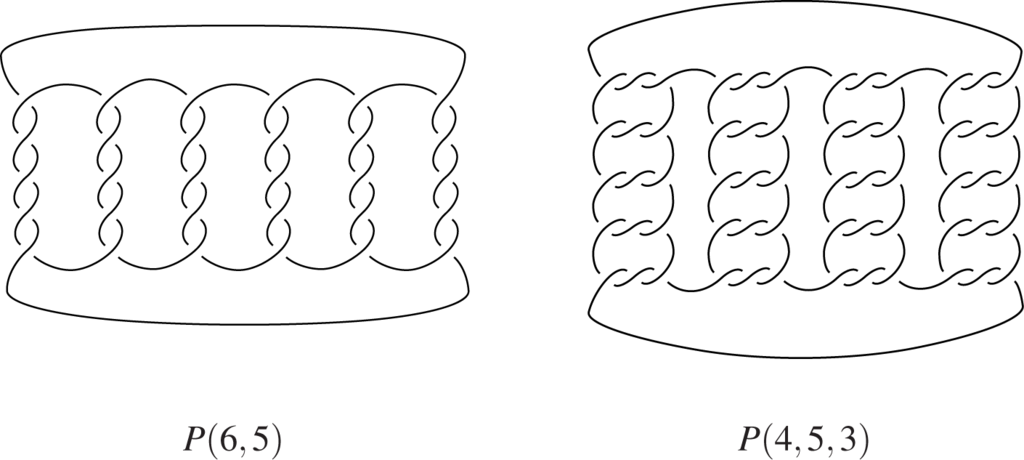
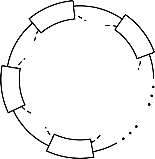
Theorem 1. A diagram D is an orientedly everywhere equivalent non-split 2-component link diagram if and only if it is among the following families:

• the pretzel link diagrams P(q, p) = (p,…, p) with q copies of p, for p,q > 0, p odd and q even, or

• the arborescent link diagrams P(q, p,3) = (P(p,3),…,P(p,3)) with q copies of P(p,3), for p > 1 odd and q > 2 even.

See Figure 1 for typical examples of either families (drawn unoriented, but any orientation will apply).

Figure 1. Examples of everywhere equivalent 2 component links.

Theorem 1 gives a sharp contrast to the rather complicated “neighboring” cases. From [1] and [2], the classification of everywhere equivalent diagrams of knots was known to be rather difficult in general. For three (or more) components, major difficulties are suggested already from the classification in another special case, this of closed 3-braids, which is worked out in a parallel paper [3].

2. Link Diagrams and Link Polynomials

All link diagrams are considered oriented, even if orientation is sometimes ignored. We also assume here that we actually regard a link diagram to live in S², that is, we consider as equivalent diagrams in the plane which differ by the choice of the point at infinity.

The Jones polynomial V ∈ ℤ [t^±1/2] is an oriented link invariant which can be specified by the skein relation

(1)

Write c(D) for the crossing number of a link diagram D. The writhe w(D) of D is the sum of the signs of all crossings of D. If all crossings of D are positive, then D is called a positive diagram.

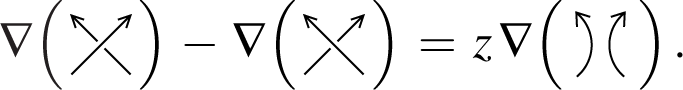
The Conway polynomial ∇ = ∇_L(z) of oriented links L satisfies $\nabla (○)=1$ and the skein relation

(2)

For a Laurent polynomial P ∈ ℤ [x,x⁻¹], let [P]_k be the coefficient of x^k in P. The minimal or maximal degree mindegP or maxdegP is the minimal or maximal exponent k ∈ ℤ of x with non-zero coefficient [P]_k. Let span_xP = maxdegP − mindegP.

Let for a link L and a diagram D of L the number n(L) = n(D) be the number of components of L or D. Then it is well known that

For knots K, i.e., n(K) = 1, this inequality is exact, and

For links, it is possible to express [∇(L)]_n(L)−1 using component linking numbers, using a formula of Hoste-Hosokawa [4,5].

In a link diagram D a crossing is a self-crossing, if both crossing strands belong to the same component. Otherwise we call the crossing mixed. The linking number lk(L_i,L_j) of two components L_i,L_j of a link L is half of the sum of the signs of all crossings between these components. Let the linking graph Λ(L) of L have L_i as vertices and an edge between L_i and L_j iff lk(L_i,L_j) ≠ 0. The Hoste-Hosokawa formula states

Lemma 2. If L is a link with a connected diagram D where all mixed crossings are of the same sign, then mindeg∇(L) = n(L) − 1.

Proof. Note that with Equation (4), the case that L is a knot fits well into the statement, so we can assume L has n(L) ≥ 2 components we denote by L_i. It is clear that all lk(L_i,Lj) ≠ 0 have the same sign. Thus in Equation (5) all products in the sum come with the same sign. The connectedness of D implies that Λ(L) is connected, and has a spanning tree. Thus at least one summand occurs. □

We will also need to recall the alternative description of the Jones polynomial V via Kauffman’s state model [6].

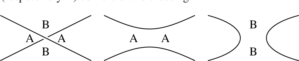
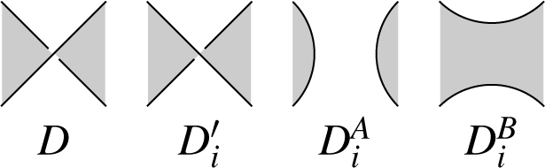
The diagrams in Figure 2 below show A- and B-corners of a crossing, and its both splittings. The corner A (respectively B) is the one passed by the overcrossing strand when rotated counterclockwise (respectively clockwise) towards the undercrossing strand. A type A (respectively B) splitting is obtained by connecting the A (respectively B) corners of the crossing.

Figure 2. Corners of a crossing and splittings.

A state S of a link diagram D is a choice of splittings of type A or B for any single crossing of D, i.e., it can be formally seen as a map S : {crossings of D} → {A,B}. When for a state S all splittings are performed, we obtain a collection of (disjoint) loops of S in the plane.

The Kauffman bracket ⟨D⟩ [6] of a link diagram D is a Laurent polynomial in a variable A, satisfying the bracket relations

(6)

By applying the first relation to each crossing of D, and then evaluating the bracket on a collection of loops using the second relation, we can express ⟨D⟩ as a sum over all states S of D:

Here #A(S) and #B(S) denote the number of type A (respectively, type B) splittings and |S| the number of loops of S. (Our normalization is thus that the diagram of one circle with no crossings has unit bracket.)

The Jones polynomial of a link L can be determined from the Kauffman bracket of some diagram D of L by

3. Everywhere Equivalence Properties for 2-Component Links

We stipulate that in general D will be used for a link diagram and D′ for a diagram obtained from D by exactly one crossing change. If we want to indicate that we switch a crossing numbered as i, we also write ${D^{\prime }}_i$.

Definition 3. We call a link diagram D everywhere equivalent if all diagrams ${D^{\prime }}_i$ depict the same link for all i. (This link may be different from the one represented by D.)

Between the rather complicated cases of knots and 3-component links, for two components it turns out that some tangible properties can be given even for arbitrary diagrams. In order to leave the subtleties for knots to their own merit, we will assume below that all link diagrams are non-split, i.e., there is no closed curve disjoint from the diagram which contains parts of it in both interior and exterior.

Component orientation issues must be taken seriously for general link diagrams (unlike the special cases treated in [3]), and thus it is helpful in the sequel to make a clear distinction.

Definition 4. We call a link diagram D orientedly everywhere equivalent if all ${D^{\prime }}_i$ depict links isotopic with orientation, up to simultaneously reversing orientation of all components. Let D be unorientedly everywhere equivalent if all D^′_i depict links isotopic as unoriented links. (Again, in either case we do not prescribe how isotopies should map between specific components; see Remark 1 below.)

We will almost exclusively consider oriented everywhere equivalence, and we will often omit the word “oriented” in the sequel. We start by observing the following necessary condition:

Lemma 5. Let D be an orientedly everywhere equivalent non-split link diagram. Then D is a knot diagram, or all components of D appear as unknotted circles (i.e., D has no self-crossings).

Proof. Since the Jones polynomial of all D′ must be equal, by the skein relation (1), so must be the Jones polynomials of the crossing-smoothed versions of D, when crossings of the same sign are smoothed out. The number of components of these diagrams is captured by the Jones polynomial (its value V(1); see e.g. Section 12 in [7]), and on the other hand it is determined by whether the two components meeting at a crossing are the same or different. Both cases can thus not occur simultaneously.

Thus one cannot have a mixed and a self-crossing of the same sign simultaneously. There must obviously be mixed crossings (when D is connected and not a knot diagram). Thus if self-crossings exist in D, then they are all positive, and all mixed crossings are negative (or vice versa; up to mirror image).

Assume that D is not a knot diagram and moreover D has self-crossings. Let D⁻ be the diagram obtained from D by smoothing a (negative) mixed crossing, and D⁺ be obtained from D by smoothing a (positive) self-crossing. The everywhere equivalence property of D and the skein relation (2) give

Now n(D⁺) = n(D) + 1, and thus from Equation (3)

On the other hand, n(D⁻) = n(D) − 1, and all mixed crossings of D′ are also mixed crossings of D, and hence have the same (here, negative) sign. Thus by Lemma 2,

With Equation (10), this contradicts Equation (9). □

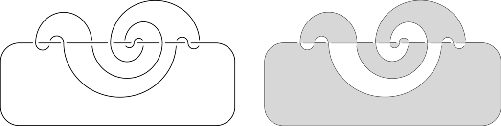
From now on we will focus on two components. We call a 2-component link diagram with no self-crossings a meander diagram. Lemma 5 then means that orientedly everywhere equivalent diagrams are meander diagrams. A typical alternating example, together with its checkerboard coloring (to be clarified and used later), is shown in Figure 3.

Figure 3. A meander diagram and its checkerboard coloring.

We call an oriented diagram special if it becomes alternating when all crossings are switched to be positive. (Another way of saying it is that there are no separating Seifert circles; cf. [8], p. 536.)

Lemma 6. Meander diagrams (with any orientation) are special.

Proof. We switch crossings in a meander diagram D so that they are positive, and we show that D is alternating. Assume D is not alternating.

Thus one component has two consecutive (say) crossing underpasses. Because of positivity, both overpass strands are oriented in the same direction. They belong to the same component, and thus they must connect in one of the two ways shown in Figure 4.

Figure 4. Connection of overpassing strands.

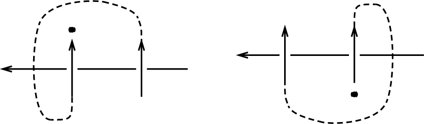
But in either case, the end marked with a bead cannot be extended to a closed component without creating self-intersections (or an intersection with the other component between the two indicated crossings). □

Lemma 7. Meander diagrams have a bigon region.

Proof. Assume the first component (circle) is drawn, and draw successively the second component. The second crossing (with the first component) will create a bigon region. To spoil this region, one must enter it, then creating a smaller bigon region. Obviously, the nesting cannot go on infinitely. □

The following equation,

(11)

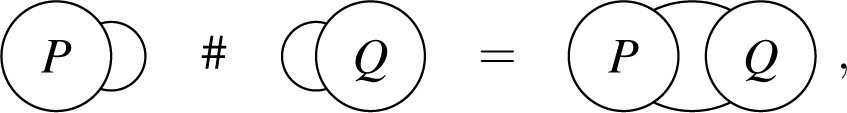
Lemma 8. Meander diagrams are prime.

Proof. If a meander diagram D is composite, then one of P, Q on the right of Equation (11) must contain just one component, and at the absence of self-crossings, be an unknotted arc. □

Lemma 9. Let D be an oriented 2-component link diagram. If D is orientedly everywhere equivalent, then it is positive (up to mirror image).

Proof. If D is orientedly everywhere equivalent, then all ${D^{\prime }}_i$ must have the same writhe $w({D^{\prime }}_i)$, since (at the absence of self-crossings) $w({D^{\prime }}_i)/2$ is the linking number of the components of ${D^{\prime }}_i$. And $w(D)-w({D^{\prime }}_i)$ is twice the sign of crossing i. □

4. Proof of Main Result

We can turn now to our main result Theorem 1. The first family the theorem includes, for p = 1, the (2,q)-torus links as a special case. For p = 1, the second family reduces to the (2,3q)-torus links, and for q = 2 to P(2p,3), which is why we excluded these values there. We showed in Figure 1 the first disambiguating instance for the second family, for q = 4 and p = 5, even although it already has 60 crossings.

Proof of Theorem 1. This proof crucially exploits (and owes its brevity to) the consequence of Lemmas 6 and 9 that if an oriented 2-component link diagram D is orientedly everywhere equivalent, then D is alternating. This allows us to put out the heavy arsenal of [6] and [9], which helps us comfortably win the battle over countless possibilities.

To clean up the argument, it is better to use induction on the crossing number. We thus check first diagrams D of, say, up to 4 crossings. For the induction step, we then fix an everywhere equivalent diagram D, and assume that all everywhere equivalent diagrams of smaller crossing number conform to the patterns in Theorem 1.

The alternation of D means that each region of D contains only A-corners or only B-corners of crossings as in Figure 2. There is a black-white coloring of the regions of D, the checkerboard coloring, which assigns different colors to each pair of regions opposite at some edge of D. (See Figure 3, or also, e.g., Figure 5 in [10], or [6,11].) Let us fix here the colors so that the A-corners of crossings lie in white regions and the B-corners in black regions, as shown in Figure 5.

Figure 5. Locally changed diagrams and their checkerboard coloring.

A crossing is nugatory if it has the same region at its both A- or its both B-corners. We call a diagram reduced if it has no nugatory crossings. It is easy to see that nugatory crossings are always self-crossings, thus in particular, D is reduced.

Now, for whatever crossing i one switches in D, the diagrams ${D^{\prime }}_i$ have the same writhe (by Lemma 9) and represent isotopic links. It follows from Equation (8) that their brackets $⟨{D^{\prime }}_i⟩$ are equal. It will turn out sufficient to just study those brackets, and since they are unoriented invariants, it is legitimate to suppress component orientation in our further treatment.

Now, superposing the first bracket relation in Equation (6) and its mirrored version (with A^±1 interchanged) with Figure 5, we see that ⟨D⟩ and $⟨{D^{\prime }}_i⟩$ determine $⟨D_i^A⟩$ and $⟨D_i^B⟩$. Therefore, $⟨D_i^A⟩$ are the same for all i, and also similarly $⟨D_i^B⟩$. It will be enough to look at the A-span of these polynomials. (That is, for our conclusion that D lies in the families descibed in Theorem 1, we will only use that the A-spans of these polynomials are equal.)

We call two crossings A (respectively B)-equivalent if they have the same pair of white (respectively black) regions. Let #_A(i) be the number of crossings A-equivalent to crossing i in D (itself included), and similarly define #_B(i).

Let for some crossing i both #_A(i) and #_B(i) be greater than 1. Thus, first, there is a crossing j ≠ i which is A-equivalent to i. This means that their two white regions coincide, and there is a closed curve γ intersecting D only in i, j, and passing through two white regions of D otherwise. Similarly, there is a closed curve γ′ intersecting D only in i, some crossing j′ ≠ i, and passing through two black regions. Both curves can intersect only at crossings of D, since they pass regions of different color. They intersect at i, and since they must intersect again, but meet only one other crossing of D, they must intersect at the same other crossing j = j′. If some of the four regions of S² \ (γ∪γ′) contains crossings of D, then D is composite, which cannot occur for meander diagrams by Lemma 8. Thus D has only the crossings i and j, and is the 2-crossing Hopf link diagram P(2,1), which was dealt with.

We assume thus now that a crossing does not simultaneously have both A- and B-equivalent other crossings in D. Then setting crossings p and q to be (twist) equivalent if they are A- or B-equivalent defines also an equivalence relation. Let us for brevity call a class (respectively A-class, respectively B-class ) an equivalence class under twist equivalence (respectively A-equivalence, respectively B-equivalence).

We will need another different description of this relation. A flype is a move on a diagram shown in Figure 6.

Figure 6. A flype at a crossing p.

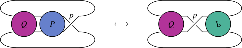
There is a natural correspondence between the crossings of two diagrams related by a flype: p moves position, and the crossings in tangles P and Q on either side of Figure 6 correspond bijectively.

Assume two crossings p, q are, say, A-equivalent. Thus there is a closed curve γ intersecting D only in p, q, and passing through two white regions of D otherwise. Then the interior of D contains a tangle, on which a flype can be applied. After this flype the interior of γ contains no crossings, and a black bigon region with corners p and q. Similarly one can argue for B-equivalent crossings. This shows that two crossings are twist equivalent (respectively A- respectively B-equivalent), if and only if there is a sequence of flypes making them form a bigon region (respectively black respectively white bigon region). We say that an equivalence class of n crossings of D is reduced, if its crossings form (at least) n − 1 bigons. Up to flypes we can achieve that every class is reduced, in which case we call the diagram twist reduced.

One important feature of flypes is that they commute with crossing changes, and that thus (both oriented and unoriented) everywhere equivalence is invariant under flypes.

Now, returning to $D_i^A$ and $D_i^B$, we observe that they are alternating. The diagram $D_i^A$ has $c(D_i^A)=c(D)-1$ crossings, but some are nugatory. These nugatory crossings are precisely the crossings A-equivalent to i in D (except for i itself, which disappeared under the splitting). Thus there are #_A(i)−1 of them in $D_i^A$. Removing these nugatory crossings, one obtains a reduced alternating diagram of c(D) − #_A(i) crossings. Similarly for $D_i^B$. We have then from the result of [6,10] that

Since we obtained that $⟨D_i^A⟩$ is equal for all i, and similarly $⟨D_i^B⟩$, it follows now that #_A(i) does not depend on the crossing i, and neither does #_B(i).

Every meander diagram must have some bigon region (Lemma 7), so that for some i, max{#_A(i),#_B(i)} > 1. Thus there is a number k > 1, such that the crossings of D decompose into equivalence classes of size k, which are either all A-classes, or all B-classes. Let us assume the latter; for the former, replace “B” by “A” in the rest of the argument. Also assume D is twist reduced, with the promise to take care of flypes later.

Let first k be even. We draw one component of D dashed, while we isotope the diagram in the plane so that the other component, drawn as a solid line, is a visible circle. We replace each B-class of D by a box. The solid line enters these boxes in some order. Since k is even, the dashed line enters each of these boxes and exits it on the same side of the solid line.

Thus we have a picture like in Figure 7. Now, all crossings of D have been included in boxes, thus we have to connect the dashed ends without self-crossings to form a component. This can be done only in the obvious way, resulting in a (2,nk)-torus link diagram, and flypes do not yield from it any further diagram.

Figure 7. Connecting boxes of even twist-equivalence classes.

If k is odd (with k ≥ 3), we use induction.

Let $\widehat{D}$ be the diagram obtained from D by replacing each B-class, numbered i, of k crossings by a single crossing, also numbered i. This means that we obtain $\widehat{D}$ from D by A-splitting k − 1 crossings in each B-class (of k crossings), i.e., so that their white regions are joined. Since k is odd, this procedure does not change the number of components, and clearly $\widehat{D}$ is a meander diagram also.

We will argue below in Lemma 10 that $\widehat{D}$ is everywhere equivalent. As $c(\widehat{D})=c(D)/k<c(D)$, by induction, $\widehat{D}$ is a diagram in Theorem 1, and D is obtained from $\widehat{D}$ by replacing each crossing with a fixed odd number k of B-equivalent crossings (for one of the two checkerboard colorings). Since the resulting diagrams D are all alternating and have an explicit shape, it is easy to test, using [9], that the everywhere equivalent ones remain in the families described in Theorem 1 (and that flypes do not yield anything new either). That is, the change from $\widehat{D}$ to D does not lead to any further everywhere equivalent diagrams.

For example, when $\widehat{D}=P(q,p)$, then, depending on the coloring, D = P(q, kp) or D = P(q, p, k). The former type is obviously nothing new, and the latter type is not everywhere equivalent when k ≥ 5. In that case, namely, all ${D^{\prime }}_i$ would simplify to alternating diagrams of two crossings less, which admit no flypes, and not all are equivalent in S² (except if p = 1 or q = 2, which are again covered before). The special role of k = 3 in the second family is that when under a crossing change the class reduces to one crossing, one can apply flypes to move it along. The case that $\widehat{D}=P(q,p,3)$ can be discussed similarly. □

Lemma 10. If D is everywhere equivalent, so is$\widehat{D}$.

Proof. Let ${\widehat{D}}_i$ and ${\widehat{D}}_j$ be the diagrams obtained from $\widehat{D}$ by switching crossings i and j. These correspond to (B-)classes numbered i and j in D.

We reduce the number of crossings in class i of D from k to k −2, obtaining a diagram D_i. Since D is everywhere equivalent and all D_i are alternating, by [9], there is a sequence of flypes carrying over D_i to D_j. Let ${\tilde{D}}_i$ be the diagram obtained from D_i by switching ⌊k/2⌋ crossings in each (B-)class of D_i. (Note that these classes have k crossings, except one, with k − 2.) It is not necessary to reduce the number of crossings in ${\tilde{D}}_i$ by removing trivial clasps by Reidemeister II moves. The flypes turning D_i to D_j carry over to transform ${\tilde{D}}_i$ into ${\tilde{D}}_j$. But ${\tilde{D}}_i$ (respectively ${\tilde{D}}_j$) depicts the same link as ${\tilde{D}}_i$ (respectively ${\tilde{D}}_j$). In fact, ${\tilde{D}}_i$ and ${\tilde{D}}_j$ also become equivalent under flypes. □

Remark 1. Note that the use of the Jones and Conway polynomial does not restrict us to (excluding) isotopies between the links of ${D^{\prime }}_i$ mapping components in prescribed ways. For example, the diagram D gives a natural bijection between components of ${D^{\prime }}_i$ and ${D^{\prime }}_j$, but this correspondence was never relevant.

Remark 2. For unoriented everywhere equivalence, the treatise grows indefinitely more complicated at several places, even though we have again concrete examples from [1] (and can suspect them to be exhaustive). For instance, the proof of Lemma 5 fails, and meander diagrams are no longer (arguably) positive, and hence neither they are alternating.

References

1. Stoimenow, A. Everywhere equivalent and everywhere different knot diagrams. Asian J. Math. 2013, 17, 95–137. [Google Scholar]
2. Stoimenow, A.; Askitas, N. On unknotting numbers and knot trivadjacency. Math. Scand. 2004, 94, 227–248. [Google Scholar]
3. Stoimenow, A. Everywhere equivalent 3-braids. Symmetry, Integrability and Geometry: Methods and Applications (SIGMA) 2014, 10. [CrossRef]
4. Hosokawa, F. On ∇-polynomials of links. Osaka Math. J 1958, 10, 273–282. [Google Scholar]
5. Hoste, J. The first coefficient of the Conway polynomial. Proc. Am. Math. Soc. 1985, 95, 299–302. [Google Scholar]
6. Kauffman, L.H. State models and the Jones polynomial. Topology 1987, 26, 395–407. [Google Scholar]
7. Jones, V.F.R. Hecke algebra representations of braid groups and link polynomials. Ann. Math. 1987, 126, 335–388. [Google Scholar]
8. Cromwell, P.R. Homogeneous links. J. Lond. Math. Soc. 1989, 39, 535–552. [Google Scholar]
9. Menasco, W.W.; Thistlethwaite, M.B. The Tait flyping conjecture. Bull. Am. Math. Soc. 1991, 25, 403–412. [Google Scholar]
10. Thistlethwaite, M.B. A spanning tree expansion for the Jones polynomial. Topology 1987, 26, 297–309. [Google Scholar]
11. Stoimenow, A. Square numbers, spanning trees and invariants of achiral knots. Commun. Anal. Geom. 2005, 13, 591–631. [Google Scholar]