Intuitionistic Fuzzy Least Square Projection Twin Support Vector Machine for Pattern Classification

Abstract

The Least Square Projection Twin Support Vector Machine (LSPTSVM) is an effective machine learning tool for solving classification problems. However, LSPTSVM does not account for the contribution of each sample during training, making it susceptible to outliers and noise. This susceptibility diminishes its generalization capability. To remedy this shortcoming, this paper introduces an Intuitionistic Fuzzy LSPTSVM (IFLSPTSVM). This model combines the LSPTSVM with the concept of Intuitionistic Fuzzy Numbers (IFN). In the training process of IFLSPTSVM, the importance of each training sample is gauged using an IFN-based score function that considers its geometric position and surrounding environment. Moreover, the weighted class mean, as opposed to the standard mean used in LSPTSVM, is employed in the calculation of intra-class scatter based on the intuitionistic fuzzy score of the sample. This approach effectively mitigates the impact of noise and outliers and more accurately captures the global information of the class samples. Experimental results on several real-world UCI benchmark datasets and the Case Western Reserve University rolling bearing datasets exhibit the efficacy of the proposed method.

1. Introduction

Based on the proximal support vector machine (PSVM) [1], Mangasarian and Wild developed the generalized eigenvalue proximal SVM (GEPSVM) [2], a fast binary classifier. Unlike PSVM, which finds two parallel hyperplanes, GEPSVM targets two non-parallel hyperplanes. Its objective is to position each hyperplane as close as possible to the corresponding class of samples, while maximizing the distance to the samples of the other class, which is achieved by solving two generalized eigenvalue problems [2]. Compared with the standard SVM [3,4], this method has lower computational complexity and delivers better classification performance on the XOR problem [2].

To enhance the generalization performance of GEPSVM, Jayadeva et al. proposed an independent non-parallel hyperplane classifier called twin support vector machines (TSVM) [5]. The algorithm aims to construct two non-parallel hyperplanes for any given binary dataset, where each hyperplane is closer to one class and at least one unit away from the other class [5]. Instead of solving a single large quadratic programming problem (QPP) required by standard SVM, TSVM solves a pair of smaller QPPs, achieving a learning speed roughly four times faster than that of standard SVM [5]. Experimental results reported in [5] show that TSVM outperforms both SVM and GEPSVM in generalization performance, i.e., classification accuracy on unseen test samples.

To further improve the classification performance of TSVM, Shao et al. developed an improved version called twin bounded support vector machines (TBSVM) [6]. The key advantage of TBSVM over TSVM is that it implements the structural risk minimization principle by adding a regularization term [6]. To further reduce the training cost of TSVM, Kumar and Gopal proposed a variant of TSVM: least squares twin support vector machines (LSTSVM) [7]. LSTSVM has an extremely fast training speed, as its separating hyperplanes are obtained by solving a single system of linear equations [7]. Numerous improved TSVM models have been proposed based on different considerations, including twin parametric-margin SVM (TPMSVM) [8], TSVM with universum (U-TSVM) [9], TSVM with pinball loss (Pin-TSVM) [10], multi-task LSTSVM (MTLSTSVM) [11], capped L1-norm TSVM (CTSVM) [12], twin K-class support vector classification with pinball loss (Pin-TKSVC) [13], and smooth pinball TSVM (SP-TSVM) [14].

If the two classes of training samples show different class scatters, TSVM may have poor generalization performance [15]. Based on the ideas of multi-weight vector projection support vector machine (MVSVM) [16] and TSVM, Chen et al. proposed the projection twin support vector machine (PTSVM) [17]. Similar to TSVM, PTSVM solves two smaller quadratic programming problems (QPPs) to obtain two projection directions, while MVSVM needs to solve two generalized eigenvalue problems [17]. Different from TSVM, PTSVM aims to find an optimal projection direction for each class instead of generating a hyperplane. Experimental results reported in [17] show that the classification performance of PTSVM is comparable to that of GEPSVM, TSVM, and MVSVM. After that, Shao et al. [18] extended PTSVM to nonlinear classification, which was not covered in the original work [17]. To reduce the computational cost of PTSVM, Shao et al. put forward the least squares PTSVM (LSPTSVM) [19]. Unlike PTSVM, which requires solving two QPPs, the solution of LSPTSVM is obtained by solving two linear equations [19]. This method enables LSPTSVM to process large datasets accurately without relying on any external optimizer [19]. Ding and Hua [20] further extended LSPTSVM to solve the nonlinear classification problem that had not been addressed in [19].

If the training dataset contains noise and outliers, LSPTSVM cannot find its two optimal hyperplanes, leading to degraded classification performance. To address the same issue that affects TSVM, Rezvani et al. [21] combined the idea of intuitionistic fuzzy number (IFN) [22,23] with TSVM and proposed the intuitionistic fuzzy TSVM (IFTSVM). An IFN consists of a membership value and a non-membership value [22]. The membership value is calculated based on the distance between a training sample and its class center, while the non-membership value is determined by the ratio of dissimilar samples to the total number of samples in the neighborhood [22]. The score function of the IFN is used to evaluate the contribution of each training sample, allowing IFTSVM to reduce the impact of noise and correctly identify support vectors from noisy data [21]. Laxmi et al. [24] extended IFTSVM by developing a least squares variant, called the intuitionistic fuzzy least squares twin support vector machine (IFLSTSVM). Instead of solving the two quadratic programming problems required by IFTSVM, this method obtains nonparallel hyperplanes by solving only two systems of linear equations, which speeds up the training process [24]. Inspired by the outstanding performance of the intuitionistic fuzzy membership scheme and GEPSVM, Quadir et al. [25] proposed the Intuitionistic Fuzzy Generalized Eigenvalue Proximal Support Vector Machine (IFGEPSVM), which solves the generalized eigenvalue problem under an intuitionistic fuzzy framework. Compared with IFTSVM, IFGEPSVM has lower computational complexity [25].

In this paper, we integrate the idea of IFN and LSPTSVM to propose a novel classification model named the intuitionistic fuzzy least square projection twin support vector machine (IFLSPTSVM), which is designed to solve binary classification problems. The key advantages of the proposed method are as follows:

• Unlike LSPTSVM, which treats all training samples as equally important, IFLSPTSVM assigns a corresponding IFN to each training sample based on its geometric position and surrounding conditions during the training process. This design reduces the susceptibility of IFLSPTSVM to interference from outliers and noise, which in turn improves the generalization performance of the model.
• When calculating intra-class scatter, IFLSPTSVM replaces the standard class mean used in LSPTSVM with a weighted class mean computed based on the IFN. This adjustment enables IFLSPTSVM to better resist the interference of noise and outliers, and more effectively capture the global information of the corresponding class samples.
• IFLSPTSVM is an extension of LSPTSVM. When the intuitionistic fuzzy score of each sample in IFLSPTSVM degenerates to 1, IFLSPTSVM reduces to the original LSPTSVM. This result demonstrates that IFLSPTSVM inherits all the advantages of LSPTSVM.
• Compared with other similar intuitionistic fuzzy-based classification models, IFLSPTSVM achieves comparable statistical performance across multiple benchmark classification tasks.

The remainder of this paper is organized as follows. Section 2 reviews related work on LSPTSVM and intuitionistic fuzzy sets. Section 3 introduces and discusses IFLSPTSVM in detail. Section 4 reports the experimental results, and Section 5 gives the concluding remarks of this paper.

2. Related Work

Consider a binary classification problem in the n-dimension real space Rⁿ. The training set of m samples is represented as {(x_j⁽ⁱ⁾, y_j)|i = 1, 2; j = 1, 2, …, m_i} where x_j⁽ⁱ⁾ denotes the jth sample in class i, y_j $\in$ {+1, −1} and m = m₁ + m₂. For simplicity, the m₁ × n matrix G and m₂ × n matrix H are used to denote the positive samples in class 1 and negative samples in class 2, respectively. X = [G; H] represents the total training samples. The feature mapping of x_i is denoted as $\varphi ({\mathit{x}}_i)$.

2.1. Least Square Projection Twin Support Vector Machine (LSPTSVM)

Unlike PTSVM [17,18], the decision function of LSPTSVM [19,20] is obtained directly from the primal problems. The primal problems of LSPTSVM only have equality constraints, as shown below:

$$\begin{array}{l}\underset{{\mathit{w}}_1, \mathsf{\xi }}{\min }\hspace{1em}{\displaystyle \frac{1}{2}}{\mathit{w}}_1^T{\mathit{M}}_1{\mathit{w}}_1+{\displaystyle \frac{c_1}{2}}{\mathsf{\xi }}^T\mathsf{\xi }+{\displaystyle \frac{c_3}{2}}{‖{\mathit{w}}_1‖}^2,\\ \mathrm{s}.\mathrm{t}.\hspace{1em}-(\mathit{H}-{\displaystyle \frac{{\mathit{e}}_2{\mathit{e}}_1^T\mathit{G}}{m_1}}){\mathit{w}}_1+\mathsf{\xi }={\mathit{e}}_2 , \end{array}$$

(1)

and

$$\begin{array}{l}\underset{{\mathit{w}}_2, \mathsf{\eta }}{\min }\hspace{1em}{\displaystyle \frac{1}{2}}{\mathit{w}}_2^T{\mathit{M}}_2{\mathit{w}}_2+{\displaystyle \frac{c_2}{2}}{\mathsf{\eta }}^T\mathsf{\eta }+{\displaystyle \frac{c_4}{2}}{‖{\mathit{w}}_2‖}^2 ,\\ \mathrm{s}.\mathrm{t}.\hspace{1em}(\mathit{G}-{\displaystyle \frac{{\mathit{e}}_1{\mathit{e}}_2^T\mathit{H}}{m_2}})+\mathsf{\eta }={\mathit{e}}_1,\end{array}$$

(2)

where

$${\mathit{M}}_1={\displaystyle \sum _{i=1}^{m_1}({\mathit{x}}_i^{(1)}-\frac{1}{m_1}{\displaystyle \sum _{j=1}^{m_1}{\mathit{x}}_j^{(1)}})}{({\mathit{x}}_i^{(1)}-{\displaystyle \frac{1}{m_1}}{\displaystyle \sum _{j=1}^{m_1}{\mathit{x}}_j^{(1)}})}^T$$

(3)

and

$${\mathit{M}}_2={\displaystyle \sum _{i=1}^{m_2}({\mathit{x}}_i^{(2)}-\frac{1}{m_2}{\displaystyle \sum _{j=1}^{m_2}{\mathit{x}}_j^{(2)}})}{({\mathit{x}}_i^{(2)}-{\displaystyle \frac{1}{m_2}}{\displaystyle \sum _{j=1}^{m_2}{\mathit{x}}_j^{(2)}})}^T$$

(4)

are two scatter matrices corresponding to class 1 and class 2, respectively, $\mathsf{\xi }$ and $\mathsf{\eta }$ are slack variables, $c_1$, $c_2$, $c_3$, $c_4$ > 0 are penalty factors, and ${\mathit{e}}_1$ and ${\mathit{e}}_2$ are vectors of ones with appropriate dimension.

On substituting the equality constraint into the objective function, the primal problems (1) and (2) are formulated as

$$\underset{{\mathit{w}}_1}{\min }\hspace{1em}{\displaystyle \frac{1}{2}}{\mathit{w}}_1^T{\mathit{M}}_1{\mathit{w}}_1+{\displaystyle \frac{c_1}{2}}{‖{\mathit{e}}_2+(\mathit{H}-{\displaystyle \frac{{\mathit{e}}_2{\mathit{e}}_1^T\mathit{G}}{m_1}}){\mathit{w}}_1‖}^2+{\displaystyle \frac{c_3}{2}}{‖{\mathit{w}}_1‖}^2,$$

(5)

and

$$\underset{{\mathit{w}}_2}{\min }\hspace{1em}{\displaystyle \frac{1}{2}}{\mathit{w}}_2^T{\mathit{M}}_2{\mathit{w}}_2+{\displaystyle \frac{c_2}{2}}{‖{\mathit{e}}_1-(\mathit{G}-{\displaystyle \frac{{\mathit{e}}_1{\mathit{e}}_2^T\mathit{H}}{m_2}}){\mathit{w}}_2‖}^2+{\displaystyle \frac{c_4}{2}}{‖{\mathit{w}}_2‖}^2 .$$

(6)

Then, the projection directions w₁ and w₂ are determined by

$${\mathit{w}}_1=-{\left({\displaystyle \frac{{\mathit{M}}_1}{c_1}}+{\left(\mathit{H}-{\displaystyle \frac{{\mathit{e}}_2{\mathit{e}}_1^T\mathit{G}}{m_1}}\right)}^T\left(\mathit{H}-{\displaystyle \frac{{\mathit{e}}_2{\mathit{e}}_1^T\mathit{G}}{m_1}}\right)+{\displaystyle \frac{c_3}{c_1}}\mathit{I}\right)}^{-1}\times {\left(\mathit{H}-{\displaystyle \frac{{\mathit{e}}_2{\mathit{e}}_1^T\mathit{G}}{m_1}}\right)}^T{\mathit{e}}_2,$$

(7)

and

$${\mathit{w}}_2={\left({\displaystyle \frac{{\mathit{M}}_2}{c_2}}+{\left(\mathit{G}-{\displaystyle \frac{{\mathit{e}}_1{\mathit{e}}_2^T\mathit{H}}{m_2}}\right)}^T\left(\mathit{G}-{\displaystyle \frac{{\mathit{e}}_1{\mathit{e}}_2^T\mathit{H}}{m_2}}\right)+{\displaystyle \frac{c_4}{c_2}}\mathit{I}\right)}^{-1}\times {\left(\mathit{G}-{\displaystyle \frac{{\mathit{e}}_1{\mathit{e}}_2^T\mathit{H}}{m_2}}\right)}^T{\mathit{e}}_1.$$

(8)

The label of a new sample x is determined by the decision function expressed as

$$Label(\mathit{x})=\underset{i=1,2}{\arg \min }\{d_i\}=\underset{i=1,2}{\arg \min }(\left|{\mathit{w}}_i^T\mathit{x}-{\mathit{w}}_i^T{\displaystyle \frac{1}{m_i}}{\displaystyle \sum _{j=1}^{m_i}{\mathit{x}}_j^{(i)}}\right|),$$

(9)

where |·| is the 1-norm.

2.2. Intuitionistic Fuzzy Membership Assignment

Given a nonempty set X, a fuzzy set D in X can be defined as

$$\mathit{D}=\{(\mathit{x},{\mu }_{\mathit{D}}(\mathit{x}),{\nu }_{\mathit{D}}(\mathit{x}))|\mathit{x}\in \mathit{X}\},$$

(10)

where $0\le {\mu }_{\mathit{D}}(\mathit{x})\le 1$, $0\le {\nu }_{\mathit{D}}(\mathit{x})\le 1$, $0\le {\mu }_{\mathit{D}}(\mathit{x})+{\nu }_{\mathit{D}}(\mathit{x})\le 1$ and ${\mu }_{\mathit{D}}(\mathit{x})$, ${\nu }_{\mathit{D}}(\mathit{x})$ represent the membership and non-membership degree of x in X belonging to D, respectively. The hesitation degree of x in X can be denoted as ${\pi }_{\mathit{D}}(\mathit{x})=1-{\mu }_{\mathit{D}}(\mathit{x})-{\nu }_{\mathit{D}}(\mathit{x})$, which is the level of uncertainty in assigning x to X.

In fuzzy theory, an intuitionistic fuzzy number (IFN) is described by membership degree, non-membership degree, and hesitation degree [22]. In order to mitigate the impact of outliers and noise in practical applications, choosing appropriate membership and non-membership functions is a critical step [22,26].

The membership function of each sample is defined as

$$\mu ({\mathit{x}}_i)=\left\{\begin{array}{c}1-{\displaystyle \frac{‖\varphi ({\mathit{x}}_i)-{\mathit{C}}^{+}‖}{r^{+}+\sigma }}, y_i=+1,\\ 1-{\displaystyle \frac{‖\varphi ({\mathit{x}}_i)-{\mathit{C}}^{-}‖}{r^{-}+\sigma }}, y_i=-1,\end{array}\right.$$

(11)

where $\sigma >0$ is an adjustable parameter, the positive class center ${\mathit{C}}^{+}$ and the negative class center ${\mathit{C}}^{-}$ are represented as

$${\mathit{C}}^{+}={\displaystyle \frac{1}{m_1}}{\displaystyle \sum _{i=1}^{m_1}\varphi ({\mathit{x}}_i)}\mathrm{and} {\mathit{C}}^{-}={\displaystyle \frac{1}{m_2}}{\displaystyle \sum _{i=1}^{m_2}\varphi ({\mathit{x}}_i)},$$

(12)

and the positive class radius $r^{+}$ and negative class radius $r^{-}$ are represented as

$$r^{+}=\underset{y_i=+1}{\max }‖\varphi ({\mathit{x}}_i)-{\mathit{C}}^{+}‖\mathrm{and} r^{-}=\underset{y_i=-1}{\max }‖\varphi ({\mathit{x}}_i)-{\mathit{C}}^{-}‖.$$

(13)

The non-membership function of each sample is defined as

$$\nu ({\mathit{x}}_i)=(1-\mu ({\mathit{x}}_i))\rho ({\mathit{x}}_i),$$

(14)

where the local neighborhood set $\rho ({\mathit{x}}_i)$ is represented as

$$\rho ({\mathit{x}}_i)={\displaystyle \frac{\left|\left\{{\mathit{x}}_j\right\}|‖\varphi ({\mathit{x}}_i)-\varphi ({\mathit{x}}_j)‖\le \beta ,y_j\ne y_i\right|}{\left|\left\{{\mathit{x}}_j\right\}|‖\varphi ({\mathit{x}}_i)-\varphi ({\mathit{x}}_j)‖\le \beta \right|}},$$

(15)

where $\beta >0$ is the neighborhood radius. The score function is defined as

$$f_i=\left\{\begin{array}{ll}{\mu }_i,& {\nu }_i=0\\ 0,& {\mu }_i\le {\nu }_i\\ (1-{\nu }_i)/(2-{\mu }_i-{\nu }_i),& \mathrm{others}.\end{array}\right.$$

(16)

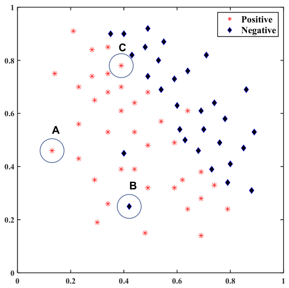
The above function can effectively distinguish support vectors from outliers and noise samples [24]. For illustration, consider the three training samples A, B, and C in Figure 1. When ${\nu }_i=0$ (i.e., positive sample A in Figure 1) and there are no negative samples in its neighborhood, the membership function can classify it accurately. When ${\mu }_i\le {\nu }_i$ (i.e., negative sample B in Figure 1), its membership value is smaller than its non-membership value, so it is treated as noise. In contrast, when ${\mu }_i>{\nu }_i$ and ${\nu }_i\ne 0$ (i.e., positive sample C in Figure 1), the sample is far away from the class center with scarce positive samples in its neighborhood, and thus should be regarded as a support vector instead of an outlier.

The membership and non-membership functions of IFN are constructed based on the inner product distance of the feature space, so the kernel function is used to construct IFN.

Theorem 1

([25]). Suppose $K({\mathit{x}}_i,{\mathit{x}}_j)$ is a kernel function. Hence, the inner product distance is presented by

$$‖\varphi ({\mathit{x}}_i)-\varphi ({\mathit{x}}_j)‖=\sqrt{K({\mathit{x}}_i,{\mathit{x}}_i)+K({\mathit{x}}_j,{\mathit{x}}_j)-2K({\mathit{x}}_i,{\mathit{x}}_j)} .$$

(17)

Theorem 2

([25]). The Euclidean distance between the sample and the corresponding class center is represented by

$$‖\varphi ({\mathit{x}}_i)-C^{+}‖=\sqrt{K({\mathit{x}}_i,{\mathit{x}}_i)+{\displaystyle \frac{1}{m_1^2}}{\displaystyle {\displaystyle \sum _{i=1}^{m_1}}{\displaystyle \sum _{j=1}^{m_1}K({\mathit{x}}_i,{\mathit{x}}_j)}}-{\displaystyle \frac{2}{m_1}}{\displaystyle {\displaystyle \sum _{j=1}^{m_1}}K({\mathit{x}}_i,{\mathit{x}}_j)}}$$

(18)

and

$$‖\varphi ({\mathit{x}}_i)-C^{-}‖=\sqrt{K({\mathit{x}}_i,{\mathit{x}}_i)+{\displaystyle \frac{1}{m_2^2}}{\displaystyle {\displaystyle \sum _{i=1}^{m_2}}{\displaystyle \sum _{j=1}^{m_2}K({\mathit{x}}_i,{\mathit{x}}_j)}}-{\displaystyle \frac{2}{m_2}}{\displaystyle {\displaystyle \sum _{j=1}^{m_2}}K({\mathit{x}}_i,{\mathit{x}}_j)}}.$$

(19)

The commonly used linear kernel function is

$$K({\mathit{x}}_i,{\mathit{x}}_j)={\mathit{x}}_i^T{\mathit{x}}_j$$

(20)

and the nonlinear kernel function is

$$K({\mathit{x}}_i,{\mathit{x}}_j)=\exp \left\{{\displaystyle \frac{-{‖{\mathit{x}}_i-{\mathit{x}}_j‖}^2}{\delta }}\right\},$$

(21)

where $\delta >0$ is a free parameter.

3. Intuitionistic Fuzzy Least Square Projection Twin Support Vector Machine

In this section, we first introduce the linear intuitionistic fuzzy LSPTSVM (IFLSPTSVM). Subsequently, we discuss several properties of the IFLSPTSVM. Finally, we extend the proposed model to the nonlinear case.

3.1. Linear IFLSPTSVM

In the linear case, IFLSPTSVM solves the following two optimization problems:

$$\begin{array}{l}\underset{{\mathit{w}}_1, \mathsf{\xi }}{\min }\hspace{1em}{\displaystyle \frac{1}{2}}{\mathit{w}}_1^T{\mathit{M}}_1{\mathit{w}}_1+{\displaystyle \frac{c_1}{2}}{\mathsf{\xi }}^T{\mathit{D}}_2\mathsf{\xi }+{\displaystyle \frac{c_3}{2}}{‖{\mathit{w}}_1‖}^2,\\ \mathrm{s}.\mathrm{t}.\hspace{1em}-\left(\mathit{H}-{\mathit{e}}_2{\mathit{h}}_1^T\mathit{G}\right){\mathit{w}}_1+\mathsf{\xi }={\mathit{e}}_2 , \end{array}$$

(22)

and

$$\begin{array}{l}\underset{{\mathit{w}}_2, \mathsf{\eta }}{\min }\hspace{1em}{\displaystyle \frac{1}{2}}{\mathit{w}}_2^T{\mathit{M}}_2{\mathit{w}}_2+{\displaystyle \frac{c_2}{2}}{\mathsf{\eta }}^T{\mathit{D}}_1\mathsf{\eta }+{\displaystyle \frac{c_4}{2}}{‖{\mathit{w}}_2‖}^2 ,\\ \mathrm{s}.\mathrm{t}.\hspace{1em}\left(\mathit{G}-{\mathit{e}}_1{\mathit{h}}_2^T\mathit{H}\right)+\mathsf{\eta }={\mathit{e}}_1,\end{array}$$

(23)

where ${\mathit{D}}_1=diag({\varphi }_1^{(1)},\dots ,{\varphi }_{m_1}^{(1)})$, ${\mathit{D}}_2=diag({\varphi }_1^{(2)},\dots ,{\varphi }_{m_2}^{(2)})$, ${\mathit{h}}_1={\left({\mathit{h}}_1^{(1)},\dots ,{\mathit{h}}_{m_1}^{(1)}\right)}^T$, ${\mathit{h}}_2={\left({\mathit{h}}_1^{(2)},\dots ,{\mathit{h}}_{m_1}^{(2)}\right)}^T$, $h_j^{(c)}={\varphi }_j^{(c)}/\left({\displaystyle \sum _{l=1}^{m_c}{\varphi }_l^{(c)}}+\epsilon \right)$, $\epsilon >0$ is an adjustable parameter, $f_j^{(c)}$ is the score of the jth sample in class c, c = 1, 2. The updated scatter matrices ${\mathit{M}}_1^{*}$ and ${\mathit{M}}_2^{*}$ are denoted as

$${\mathit{M}}_1^{*}={\displaystyle \sum _{i=1}^{m_1}\left({\mathit{x}}_i^{(1)}-{\displaystyle \sum _{j=1}^{m_1}{h}_j^{(1)}{\mathit{x}}_j^{(1)}}\right)}{\left({\mathit{x}}_i^{(1)}-{\displaystyle \sum _{j=1}^{m_1}{h}_j^{(1)}{\mathit{x}}_j^{(1)}}\right)}^T$$

(24)

and

$${\mathit{M}}_2^{*}={\displaystyle \sum _{i=1}^{m_2}\left({\mathit{x}}_i^{(2)}-{\displaystyle \sum _{j=1}^{m_2}{h}_j^{(2)}{\mathit{x}}_j^{(2)}}\right)}{\left({\mathit{x}}_i^{(2)}-{\displaystyle \sum _{j=1}^{m_2}{h}_j^{(2)}{\mathit{x}}_j^{(2)}}\right)}^T.$$

(25)

Note that IFLSPTSVM makes two extra modifications of LSPTSVM. Consider the objective function in the optimization problem (23). The first modification is that the improved scatter matrix ${\mathit{M}}_1^{*}$ is used in the objective function to account for the global information of positive samples. Based on the intuitionistic fuzzy score of the sample, the weighted class center is used in ${\mathit{M}}_1^{*}$, which can better overcome the influence of noise and outliers and better characterize the global information of positive samples. When calculating the traditional scatter matrix ${\mathit{M}}_1$, a simple arithmetic mean is adopted as the class centroid, where all samples (including noise and outliers) contribute equally to the centroid. Since noise lies far away from normal sample clusters, they directly pull the class mean away from the true center of the samples. If the scatter matrix is solved based on such biased ordinary centroids, the intra-class divergence will be falsely magnified. This not only distorts the distribution characteristics of each single class but also damages the separability between two classes, failing to reflect the real global distribution of clean samples. In contrast, for the IFN-based weighting strategy, clean samples are assigned weights close to 1, while noises and abnormal points obtain weights approaching 0. The weighted mean is dominated by mainstream normal samples and free from the offset interference caused by outliers. Constructing the scatter matrix ${\mathit{M}}_1^{*}$ with weighted class centroids as benchmarks, the calculated intra-class deviation only characterizes the genuine dispersion degree of valid samples. It avoids distribution distortion induced by noise and completely retains the global structural information of sample clusters in each class, thus exhibiting remarkably stronger noise robustness than the conventional scatter matrix with equal-weighted centroids. The weighted class center is also used in the constraint to maintain consistency. The second modification is to multiply the score for each sample in the negative class by the classification error associated with that sample to ensure that if a sample is severely misclassified, its impact is reduced by assigning a smaller score to that sample.

By substituting the equality constraint into the objective function, Equation (22) becomes

$$\begin{array}{l}\underset{{\mathit{w}}_1}{\min }\hspace{1em}{\displaystyle \frac{1}{2}}{\mathit{w}}_1^T{\mathit{M}}_1{\mathit{w}}_1+{\displaystyle \frac{c_1}{2}}{\left({\mathit{e}}_2+\left(\mathit{H}-{\mathit{e}}_2{\mathit{h}}_1^T\mathit{G}\right){\mathit{w}}_1\right)}^T{\mathit{D}}_2\left({\mathit{e}}_2+\left(\mathit{H}-{\mathit{e}}_2{\mathit{h}}_1^T\mathit{G}\right){\mathit{w}}_1\right)+\\ \hspace{1em}\hspace{1em} {\displaystyle \frac{c_3}{2}}{‖{\mathit{w}}_1‖}^2.\end{array}$$

(26)

Setting the gradient of Equation (26) with respect to ${\mathit{w}}_1$ equal to zero gives

$${\mathit{w}}_1=-{\left({\displaystyle \frac{{\mathit{M}}_1}{c_1}}+{\left(\mathit{H}-{\mathit{e}}_2{\mathit{h}}_1^T\mathit{G}\right)}^T{\mathit{D}}_2\left(\mathit{H}-{\mathit{e}}_2{\mathit{h}}_1^T\mathit{G}\right)+{\displaystyle \frac{c_3}{c_1}}\mathit{I}\right)}^{-1}{\left(\mathit{H}-{\mathit{e}}_2{\mathit{h}}_1^T\mathit{G}\right)}^T{\mathit{D}}_2{\mathit{e}}_2.$$

(27)

In exactly the same way, we can obtain ${\mathit{w}}_2$ from Equation (23), which is given by

$${\mathit{w}}_2={\left({\displaystyle \frac{{\mathit{M}}_2}{c_2}}+{\left(\mathit{G}-{\mathit{e}}_1{\mathit{h}}_2^T\mathit{H}\right)}^T{\mathit{D}}_1\left(\mathit{G}-{\mathit{e}}_1{\mathit{h}}_2^T\mathit{H}\right)+{\displaystyle \frac{c_4}{c_2}}\mathit{I}\right)}^{-1}{\left(\mathit{G}-{\mathit{e}}_1{\mathit{h}}_2^T\mathit{H}\right)}^T{\mathit{D}}_1{\mathit{e}}_1.$$

(28)

The label of a new sample x can be determined by

$$Label(\mathit{x})=\underset{i=1,2}{\arg \min }\{d_i\}=\underset{i=1,2}{\arg \min }(\left|{\mathit{w}}_i^T\mathit{x}-{\mathit{w}}_i^T{\displaystyle \sum _{j=1}^{m_i}{\mathit{h}}_j^{(i)}{\mathit{x}}_j^{(i)}}\right|).$$

(29)

3.2. Nonlinear IFLSPTSVM

In this subsection, we extend the previously discussed linear IFLSPTSVM to the nonlinear domain. By employing the kernel trick, the nonlinear IFLSPTSVM addresses the following two optimization problems:

$$\begin{array}{l}\underset{{\mathit{u}}_1, \mathsf{\xi }}{\min }\hspace{1em}{\displaystyle \frac{1}{2}}{\mathit{u}}_1^T{\mathit{M}}_1^{\varphi }{\mathit{u}}_1+{\displaystyle \frac{c_1}{2}}{\mathsf{\xi }}^T{\mathit{D}}_2\mathsf{\xi }+{\displaystyle \frac{c_3}{2}}{‖{\mathit{u}}_1‖}^2,\\ \mathrm{s}.\mathrm{t}.\hspace{1em}-(K(\mathit{H},{\mathit{X}}^T)-{\mathit{e}}_2{\mathit{h}}_1^{T}K(\mathit{G},{\mathit{X}}^T)){\mathit{u}}_1+\mathsf{\xi }={\mathit{e}}_2,\end{array}$$

(30)

and

$$\begin{array}{l}\underset{{\mathit{u}}_2, \mathsf{\eta }}{\min }\hspace{1em}{\displaystyle \frac{1}{2}}{\mathit{u}}_2^T{\mathit{M}}_2^{\varphi }{\mathit{u}}_2+{\displaystyle \frac{c_2}{2}}{\mathsf{\eta }}^T{\mathit{D}}_1\mathsf{\eta }+{\displaystyle \frac{c_4}{2}}{‖{\mathit{u}}_2‖}^2,\\ \mathrm{s}.\mathrm{t}.\hspace{1em}(K(\mathit{G},{\mathit{X}}^T)-{\mathit{e}}_1{\mathit{h}}_2^{T}K(\mathit{H},{\mathit{X}}^T)){\mathit{u}}_2+\mathsf{\eta }\ge {\mathit{e}}_1,\end{array}$$

(31)

where the scatter matrices ${\mathit{M}}_1^{\varphi }$ and ${\mathit{M}}_2^{\varphi }$ are denoted as

$${\mathit{M}}_1^{\varphi }={\displaystyle \sum _{i=1}^{m_1}\left(K({\mathit{x}}_i^{(1)},{\mathit{X}}^T)-{\displaystyle \sum _{j=1}^{m_1}{\mathit{h}}_j^{(1)}K({\mathit{x}}_j^{(1)},{\mathit{X}}^T)}\right)}\times {\left(K({\mathit{x}}_i^{(1)},{\mathit{X}}^T)-{\displaystyle \sum _{j=1}^{m_1}{\mathit{h}}_j^{(1)}K({\mathit{x}}_j^{(1)},{\mathit{X}}^T)}\right)}^T$$

(32)

and

$${\mathit{M}}_2^{\varphi }={\displaystyle \sum _{i=1}^{m_2}\left(K({\mathit{x}}_i^{(2)},{\mathit{X}}^T)-{\displaystyle \sum _{j=1}^{m_2}{\mathit{h}}_j^{(2)}K({\mathit{x}}_j^{(2)},{\mathit{X}}^T)}\right)}\times {\left(K({\mathit{x}}_i^{(2)},{\mathit{X}}^T)-{\displaystyle \sum _{j=1}^{m_2}{\mathit{h}}_j^{(2)}K({\mathit{x}}_j^{(2)},{\mathit{X}}^T)}\right)}^T.$$

(33)

Similar to the above linear case, the pair of projection vectors in the feature space can be obtained from

$$\begin{array}{ll}{\mathit{u}}_1=& -{\left({\displaystyle \frac{{\mathit{M}}_1^{\varphi }}{c_1}}+{\left(K(\mathit{H},{\mathit{X}}^T)-{\mathit{e}}_2{\mathit{h}}_1^{T}K(\mathit{G},{\mathit{X}}^T)\right)}^T{\mathit{D}}_2\left(K(\mathit{H},{\mathit{X}}^T)-{\mathit{e}}_2{\mathit{h}}_1^{T}K(\mathit{G},{\mathit{X}}^T)\right)+{\displaystyle \frac{c_3}{c_1}}\mathit{I}\right)}^{-1}\times \\ & {\left(K(\mathit{H},{\mathit{X}}^T)-{\mathit{e}}_2{\mathit{h}}_1^{T}K(\mathit{G},{\mathit{X}}^T)\right)}^T{\mathit{D}}_2{\mathit{e}}_2.\end{array}$$

(34)

and

$$\begin{array}{ll}{\mathit{u}}_2=& -{\left({\displaystyle \frac{{\mathit{M}}_2^{\varphi }}{c_2}}+{\left(K(\mathit{G},{\mathit{X}}^T)-{\mathit{e}}_1{\mathit{h}}_2^{T}K(\mathit{H},{\mathit{X}}^T)\right)}^T{\mathit{D}}_2\left(K(\mathit{G},{\mathit{X}}^T)-{\mathit{e}}_1{\mathit{h}}_2^{T}K(\mathit{H},{\mathit{X}}^T)\right)+{\displaystyle \frac{c_4}{c_2}}\mathit{I}\right)}^{-1}\times \\ & {\left(K(\mathit{G},{\mathit{X}}^T)-{\mathit{e}}_1{\mathit{h}}_2^{T}K(\mathit{H},{\mathit{X}}^T)\right)}^T{\mathit{D}}_1{\mathit{e}}_1.\end{array}$$

(35)

Then, the label of a new sample x can be determined by

$$Label(\mathit{x})=\underset{i=1,2}{\arg \min }\{d_i\}=\underset{i=1,2}{\arg \min }(\left|{\mathit{u}}_i^{T}K(\mathit{x},{\mathit{X}}^T)-{\mathit{u}}_i^T{\displaystyle \sum _{j=1}^{m_i}{\mathit{h}}_j^{(i)}K({\mathit{x}}_j^{(i)},{\mathit{X}}^T)}\right|).$$

(36)

3.3. Complexity Analysis of IFLSPTSVM

Suppose m₁ = m₂; the main computation of IFLSPTSVM consists of two steps:

(1)

Calculation of the intuitionistic fuzzy score for each training sample. In order to obtain the intuitionistic fuzzy score of each training sample, IFLSPTSVM needs to calculate the membership and non-membership values of the corresponding sample according to Equation (11) and Equation (14), respectively. In the process of calculating the membership values of training samples, it is necessary to first calculate the class center, class radius, and the distance between each class center and the samples in the class, and then use Equation (11) to calculate the membership value of each sample, which requires O(1) + O(1) + O(m₁) + O(m₁). The measure of non-membership value requires the computation of Equation (15), which requires O((m₁)²) operations. Therefore, IFLSPTSVM involves O(1) + O(1) + O(m₁) + O(m₁) + O((m₁)²) operations to measure the intuitionistic fuzzy score of training samples, which is O((m₁)²) when m₁ extends to infinity.

(2)

The optimization of IFLSPTSVM. This step for IFLSPTSVM costs around O(2(m₁)²).

Thus, the overall computational complexity of IFLSPTSVM is about O(3(m₁)²). Compared with LSPTSVM, IFLSPTSVM needs to calculate the intuitionistic fuzzy score for each training sample in the training stage, which incurs an extra cost of O((m₁)²). That is, IFLSPTSVM is slightly slower than LSPTSVM.

Unlike the linear model optimized in the original feature space, the nonlinear IFLSPTSVM projects original low-dimensional samples into a high-dimensional feature space via a kernel function, which requires the construction of a full 2 × m₁ × m₁ kernel matrix. Each element of the kernel matrix corresponds to the similarity measurement between two training samples, leading to a time complexity of O(2(m₁)²) for kernel matrix generation. Meanwhile, storing the dense kernel matrix occupies O(2(m₁)²) memory resources, which constitutes an inevitable spatial overhead that does not exist in the linear IFLSPTSVM.

4. Experimental Results

To evaluate the effectiveness and generalization capability of the IFLSPTSVM, a series of experiments are conducted systematically on several real-world UCI benchmark datasets [27] and the Case Western Reserve University (CWRU) rolling bearing datasets [28]. In the experiments, we focus on the comparison between the proposed method and some state-of-the-art classification methods, including LSPTSVM [19,20], IFTSVM [21], IFLSTSVM [24], and IFGEPSVM [25]. The entire experiments are performed using MATLAB 2024b on a desktop PC with an Intel(R) Core i7 processor (2.5 GHz) and 32 GB RAM. The optimal values of the regularization and penalty parameters for all the above algorithms are searched from the set {2ⁱ|i = −8, −7, …, 8}. To reduce the computational complexity of parameter selection, we set c₁ = c₂ and c₃ = c₄ in all algorithms. For each algorithm with nonlinear kernels, the Gaussian kernel given by K(x_i, x_j) was selected. The kernel parameter $\delta$ was searched from the set {2ⁱ|i = −1, 0, …, 7}. “Acc.” signifies the mean value of the cross-validation testing results, along with the standard deviation. “Time” denotes the average training time, measured in seconds.

4.1. UCI Datasets

In this subsection, experiments are conducted on real-world UCI benchmark datasets to compare our proposed IFLSPTSVM with LSPTSVM, IFTSVM, IFLSTSVM, and IFGEPSVM. The performance of each algorithm is estimated by the standard ten-fold cross-validation methodology. Hyperparameters are tuned by ten-fold cross-validation over the whole dataset to yield one group of global optimal hyperparameters, which are kept fixed in the ten-fold cross-validation. The averaged metrics across ten test folds are reported.

Table 1. Classification comparison for IFLSPTSVM versus LSPTSVM, IFTSVM, IFGEPSVM, and IFLSTSVM with a linear kernel.

Data Set (m × n)	IFLSTSVM Acc. Time	IFGEPSVM Acc. Time	IFTSVM Acc. Time	LSPTSVM Acc. Time	IFLSPTSVM Acc. Time
Wdbc (569 × 30)	97.55 ± 1.61 0.042	96.27 ± 3.45 0.023	97.55 ± 1.61 0.269	98.09 ± 1.64 0.004	98.42 ± 1.68 0.064
Ionosphere (351 × 34)	87.12 ± 5.47 0.047	79.92 ± 7.00 0.063	87.05 ± 7.22 0.234	91.69 ± 5.2 0.011	91.76 ± 5.39 0.017
Hepatitis (155 × 19)	86.33 ± 7.95 0.016	85.17 ± 7.76 0.016	86.83 ± 8.18 0.078	84.83 ± 7.69 0.002	87.33 ± 7.57 0.006
P_gene (106 × 57)	75.88 ± 14.34 0.016	69.38 ± 17.56 0.031	78.88 ± 13.09 0.063	76.88 ± 12.76 0.002	79.50 ± 13.5 0.003
Spect (267 × 22)	80.49 ± 3.65 0.031	68.37 ± 15.12 0.016	81.64 ± 2.29 0.253	82.03 ± 7.88 0.008	85.19 ± 8.69 0.025
Heart (270 × 13)	84.81 ± 4.81 0.016	82.96 ± 5.79 0.031	84.81 ± 4.81 0.152	84.07 ± 5.51 0.011	85.56 ± 4.81 0.020
Wpbc (198 × 33)	81.77 ± 8.28 0.063	77.5 ± 6.28 0.016	82.51 ± 7.15 0.031	78.56 ± 7.62 0.005	81.46 ± 6.82 0.019
Votes (435 × 16)	95.79 ± 2.64 0.023	95.85 ± 2.84 0.016	95.79 ± 2.64 0.114	95.08 ± 2.59 0.014	96.03 ± 2.47 0.031
Iris_23 (100 × 4)	97.0 ± 4.58 0.017	96.0 ± 6.63 0.014	97.0 ± 6.4 0.016	96.0 ± 6.63 0.002	98.0 ± 6.0 0.016
Glass_12 (146 × 9)	73.29 ± 13.19 0.002	71.64 ± 13.53 0.002	71.86 ± 12.92 0.022	66.14 ± 11.8 0.000	76.07 ± 9.04 0.003
Average rank	2.95	4.45	2.75	3.65	1.2

shows the average classification accuracy and training time of the above five algorithms in the linear case. As can be seen from Table 1, compared with the original LSPTSVM, the proposed IFLSPTSVM has a significantly higher classification accuracy. At the same time, compared with the three recently proposed intuitionistic fuzzy-based classification algorithms, including IFTSVM, IFLSTSVM, and IFGEPSVM, IFLSPTSVM has comparable classification performance. In terms of training time, our proposed IFLSPTSVM performs similarly to IFGEPSVM and IFLSTSVM, and all three methods are faster than IFTSVM, which requires solving two dual quadratic programming problems during training. However, the training speed of our IFLSPTSVM is slightly slower than that of LSPTSVM, which is mainly caused by the extra computational overhead for calculating the score of each sample.

Table 2. Classification comparison for IFLSPTSVM versus LSPTSVM, IFTSVM, IFGEPSVM, and IFLSTSVM with a nonlinear kernel.

Data Set (m × n)	IFLSTSVM Acc. Time	IFGEPSVM Acc. Time	IFTSVM Acc. Time	LSPTSVM Acc. Time	IFLSPTSVM Acc. Time
Spect (267 × 22)	85.87 ± 6.6 0.0516	83.87 ± 8.91 0.0969	85.57 ± 6.85 0.1563	83.18 ± 8.44 0.0281	85.87 ± 5.08 0.0672
Cleve (296 × 13)	85.12 ± 5.56 0.0578	81.39 ± 5.61 0.2734	84.43 ± 6.01 0.3469	84.15 ± 3.84 0.0344	85.35 ± 5.74 0.0438
Vertebral (310 × 6)	86.77 ± 6.2 0.0676	79.68 ± 6.77 0.3281	86.77 ± 5.85 0.2219	84.84 ± 5.21 0.0453	86.13 ± 6.3 0.0656
Sonar (208 × 60)	71.64 ± 13.04 0.0364	70.21 ± 20.35 0.1422	69.64 ± 18.37 0.0844	72.79 ± 14.41 0.0281	72.29 ± 15.74 0.0469
Votes (435 × 16)	96.03 ± 2.69 0.1672	91.57 ± 3.62 0.7063	96.03 ± 2.47 0.2844	96.03 ± 2.47 0.1141	96.27 ± 2.49 0.1750
Iris_23 (100 × 4)	98.00 ± 6.0 0.0156	95.00 ± 9.22 0.0250	97.00 ± 4.58 0.0375	98.00 ± 6.0 0.0016	98.00 ± 6.0 0.0125
Glass_12 (146 × 9)	80.43 ± 10.32 0.0094	74.36 ± 9.07 0.0359	81.14 ± 10.89 0.0531	78.43 ± 7.3 0.0047	82.07 ± 11.61 0.0063
Sobar (72 × 19)	93.17 ± 9.39 0.0141	91.75 ± 9.33 0.0234	90.32 ± 9.05 0.0531	90.32 ± 11.08 0.0016	93.17 ± 9.39 0.0156
Tic_tac_toe (958 × 9)	75.63 ± 7.55 0.9750	72.5 ± 10.77 3.5375	75.75 ± 6.57 1.0969	74.65 ± 9.4 0.5813	75.85 ± 10.03 0.8953
Australian (690 × 14)	87.14 ± 2.53 0.4936	87.67 ± 2.73 1.4609	87.16 ± 4.15 0.7219	87.41 ± 3.87 0.3234	87.58 ± 2.08 0.4656
Average rank	2.6	4.2	3.05	3.35	1.4

gives the average classification accuracy and training time of these algorithms in the nonlinear case. From Table 2, we can get similar conclusions.

To conduct a statistical comparative analysis of the proposed IFLSPTSVM against LSPTSVM, IFTSVM, IFLSTSVM, and IFGEPSVM, we employed the Friedman test [29] to evaluate the five algorithms across ten benchmark datasets, with corresponding p-values calculated via the tool available at https://www.graphpad.com/quickcalcs/pvalue2/, accessed on 27 August 2026. In this test, we rank each algorithm individually for every dataset. Thus

$${\chi }_F^2={\displaystyle \frac{12a}{b(b+1)}}\left[{\displaystyle \sum _{i=1}^b{r}_i^2-\frac{b{(b+1)}^2}{4}}\right],$$

(37)

is based on a ${\chi }_F^2$ distribution with degrees of freedom (b − 1) and (b − 1) (a − 1) when a and b are sufficiently large. The average rank of algorithms is $r_i$. Also, N and d are the numbers of datasets and algorithms, respectively. The Friedman ${\chi }_F^2$ produced an advisable statistic

$$F_F={\displaystyle \frac{(a-1){\chi }_F^2}{a(b-1)-{\chi }_F^2}}.$$

(38)

To evaluate the performance of the proposed IFLSPTSVM against the other four methods, we calculate the rank of each algorithm on each dataset individually (see Table 1). With a = 5 and b = 10, we calculated the Friedman statistic from the data in Table 1 under the null hypothesis, obtaining ${\chi }_F^2$ = 24.02 and $F_F$ = 13.53, where $F_F$ follows an F-distribution with (b − 1) = (10 − 1) = 9 and (b − 1) (a − 1) = (10 − 1) (5 − 1) = 36 degrees of freedom. The critical value of F(9, 36) at $\alpha$ = 0.05 is 2.15. Therefore, we reject the null hypothesis and claim that the compared algorithms are not equivalent at $\alpha$ = 0.05, i.e., $F_F$ = 13.53 > 2.15. Since we have rejected the null hypothesis, we apply the p-value test to examine the significance level of the difference. The value of $\alpha$ is set to 0.05 for the statistical test. Accordingly, if the p-value is less than 0.05, there is a significant difference between the proposed technique and the other algorithms. A smaller p-value indicates a more statistically significant difference. The p-value calculated from F(9, 36) is less than 0.0001. By conventional criteria, this difference is considered extremely statistically significant. We therefore conclude that the proposed algorithm IFLSPTSVM performs significantly better than LSPTSVM, IFTSVM, IFLSTSVM, and IFGEPSVM. In the nonlinear case, we can obtain similar results from Table 2.

To verify the effectiveness of using weighted mean in the scatter matrix, we name the version of IFLSPTSVM that uses the standard mean IFLSPTSVM-SM.

Table 3. Classification comparison for IFLSPTSVM versus IFLSPTSVM-SM.

Data Set (m × n)	The Linear Case		The Nonlinear Case
	IFLSTSVM Acc.	IFGEPSVM-SM Acc.	IFLSTSVM Acc.	IFGEPSVM-SM Acc.
Spect (267 × 22)	85.19 ± 8.69	82.03 ± 16.50	85.87 ± 5.08	83.57 ± 7.07
Ionosphere (351 × 34)	91.76 ± 5.39	91.39 ± 5.92	93.08 ± 5.18	92.79 ± 5.52
Vertebral (310 × 6)	83.87 ± 6.45	83.87 ± 7.36	86.13 ± 6.3	85.81 ± 5.62
Parkinsons (195 × 22)	84.7 ± 11.11	83.33 ± 11.11	90.56 ± 11.12	90.56 ± 11.12
Australian (690 × 14)	86.26 ± 5.03	86.26 ± 5.11	87.58 ± 2.08	87.56 ± 5.25
Hepatitis (155 × 19)	87.33 ± 7.57	86.00 ± 8.14	87.17 ± 7.6	86.5 ± 6.69

compares the classification performance of the two methods under both linear and nonlinear cases. The experimental results show that IFLSPTSVM generally outperforms IFLSPTSVM-SM, which confirms the effectiveness of adopting weighted mean to calculate the scatter matrix.

The IFTSVM, IFLSTSVM, IFGEPSVM, and our proposed IFLSPTSVM models are primarily designed to mitigate the adverse effects of noise. For a comprehensive analysis, we introduced varying levels of label noise, specifically 5%, 10%, 15%, and 20%, to deliberately corrupt the labels of these datasets. As can be seen from

Table 4. Classification comparison for IFLSPTSVM versus LSPTSVM, IFGEPSVM, IFTSVM, and IFLSTSVM under different noise ratios.

Data Set (m × n)	Ratio	IFLSPTSVM Acc.	LSPTSVM Acc.	IFGEPSVM Acc.	IFTSVM Acc.	IFLSTSVM Acc.
Wdbc (569 × 30)	5%	97.91 ± 1.29	97.91 ± 1.52	96.27 ± 3.96	96.84 ± 2.37	97.22 ± 1.73
	10%	97.57 ± 2.05	96.88 ± 2.12	95.63 ± 3.71	97.19 ± 2.13	97.37 ± 1.81
	15%	97.04 ± 2.05	96.55 ± 2.54	94.9 ± 2.59	96.84 ± 2.08	97.01 ± 1.38
	20%	97.01 ± 1.38	95.94 ± 2.79	93.8 ± 2.96	96.84 ± 1.55	97.01 ± 1.6
Ionosphere (351 × 34)	5%	91.10 ± 3.67	89.63 ± 5.07	80.43 ± 5.72	86.54 ± 6.08	87.12 ± 6.49
	10%	89.56 ± 4.18	87.79 ± 6.17	81.54 ± 5.19	88.52 ± 4.82	87.35 ± 5.26
	15%	88.38 ± 4.38	86.91 ± 8.17	81.38 ± 7.85	86.39 ± 6.38	86.76 ± 5.77
	20%	88.38 ± 4.18	86.02 ± 6.55	79.77 ± 5.28	86.69 ± 5.03	85.95 ± 6.71
Spect (267 × 22)	5%	85.19 ± 7.41	83.95 ± 7.22	72.82 ± 7.67	80.10 ± 7.07	81.64 ± 5.10
	10%	85.87 ± 6.37	83.65 ± 8.31	70.29 ± 7.81	79.72 ± 17.64	81.18 ± 17.92
	15%	85.41 ± 8.74	83.18 ± 6.9	71.91 ± 9.29	80.87 ± 6.31	82.41 ± 12.42
	20%	85.71 ± 12.03	85.1 ± 5.75	72.13 ± 8.20	81.48 ± 2.13	82.63 ± 12.64
Heart (270 × 13)	5%	85.56 ± 5.60	84.81 ± 5.35	82.92 ± 6.24	85.56 ± 5.60	85.19 ± 5.74
	10%	85.93 ± 4.91	84.44 ± 5.44	82.22 ± 4.91	85.56 ± 5.09	85.56 ± 4.81
	15%	85.56 ± 4.81	84.44 ± 3.63	82.22 ± 5.44	85.56 ± 5.09	85.56 ± 4.21
	20%	84.81 ± 4.52	84.07 ± 5.75	82.22 ± 5.19	84.44 ± 3.63	84.81 ± 4.52
Iris_23 (100 × 4)	5%	98.00 ± 6.00	95.00 ± 6.71	95.00 ± 6.71	97.00 ± 6.40	97.00 ± 6.40
	10%	97.00 ± 6.40	95.00 ± 6.71	96.00 ± 6.63	96.00 ± 6.63	96.00 ± 6.63
	15%	96.00 ± 6.63	95.00 ± 6.71	95.00 ± 6.71	96.00 ± 6.63	96.00 ± 6.63
	20%	95.00 ± 5.00	95.00 ± 5.00	94.00 ± 6.63	95.00 ± 6.71	95.00 ± 6.71
Glass_12 (146 × 9)	5%	74.64 ± 7.22	63.21 ± 8.76	69.00 ± 13.09	70.64 ± 14.01	72.79 ± 14.85
	10%	73.93 ± 9.04	63.50 ± 15.70	68.00 ± 13.00	71.86 ± 11.68	73.29 ± 11.54
	15%	67.93 ± 10.20	63.71 ± 17.75	65.14 ± 8.36	72.07 ± 12.48	74.00 ± 11.62
	20%	66.21 ± 17.92	65.07 ± 19.55	66.07 ± 11.66	72.5 ± 12.17	71.57 ± 12.46
Sobar (72 × 19)	5%	93.17 ± 6.88	88.89 ± 8.52	87.46 ± 10.0	92.86 ± 7.14	94.6 ± 6.67
	10%	90.32 ± 9.05	88.89 ± 10.65	83.17 ± 10.82	91.43 ± 11.43	88.89 ± 8.52
	15%	87.46 ± 13.48	82.06 ± 15.42	72.38 ± 24.36	80.32 ± 16.05	79.21 ± 18.2
	20%	80.32 ± 20.51	78.57 ± 24.12	71.75 ± 29.45	77.46 ± 19.54	79.21 ± 17.04
Hepatitis (155 × 19)	5%	88.50 ± 7.97	84.67 ± 12.67	85.00 ± 11.86	86.83 ± 8.18	86.83 ± 7.01
	10%	87.50 ± 7.86	86.17 ± 6.67	85.67 ± 10.96	87.50 ± 7.27	87.50 ± 7.86
	15%	87.50 ± 4.90	85.67 ± 12.12	85.83 ± 5.54	87.83 ± 7.23	87.17 ± 6.99
	20%	86.50 ± 7.90	87.33 ± 5.54	86.00 ± 8.67	87.33 ± 6.56	88.33 ± 6.54
P_gene (106 × 57)	5%	78.88 ± 14.54	75.25 ± 9.90	68.15 ± 16.13	77.50 ± 12.50	74.50 ± 12.74
	10%	74.50 ± 16.19	72.50 ± 13.28	67.00 ± 14.18	76.50 ± 8.96	69.12 ± 12.32
	15%	73.50 ± 10.97	64.87 ± 14.28	67.25 ± 12.57	72.50 ± 7.50	73.75 ± 12.51
	20%	67.13 ± 13.58	58.88 ± 16.32	63.63 ± 15.11	66.50 ± 7.09	63.13 ± 16.52
Votes (435 × 16)	5%	95.79 ± 2.64	95.79 ± 2.64	95.79 ± 2.64	96.03 ± 2.47	96.03 ± 2.47
	10%	95.79 ± 2.64	95.79 ± 2.64	95.79 ± 2.64	95.79 ± 2.64	95.79 ± 2.64
	15%	95.79 ± 2.64	95.79 ± 2.64	95.85 ± 2.84	95.85 ± 3.03	96.03 ± 2.69
	20%	95.79 ± 2.64	95.20 ± 3.28	95.79 ± 2.64	95.79 ± 2.64	95.79 ± 2.64

, the overall recognition accuracy of all methods shows a declining trend as the noise ratio increases. Compared with LSPTSVM, the proposed IFLSPTSVM achieves significantly better classification performance, which demonstrates that the introduction of the IFN idea can indeed improve the anti-noise capability of the algorithm. Compared with the similar IFTSVM, IFLSTSVM, and IFGEPSVM, our proposed IFLSPTSVM achieves better classification performance on most datasets. Overall, IFLSPTSVM can operate efficiently on datasets with different noise ratios and significantly mitigate the influences of outliers and noise.

4.2. CWRU Datasets

In this subsection, experiments are conducted on the CWRU rolling-bearing datasets [28] to compare the classification performance of the proposed IFLSPTSVM with LSPTSVM, IFTSVM, IFLSTSVM, and IFGEPSVM. The CWRU datasets have been widely used in fault-diagnosis research for more than ten years. The bearing adopted in this paper is the SKF-6205 deep-groove ball bearing. The fault diameters are 0.007 inches, 0.014 inches, and 0.021 inches, respectively, with a fault depth of 0.011 inches, a load of 3 horsepower, and a sampling frequency of 12 kHz. The sampling position is located at the drive end. Ten groups of data are considered in the experiments. Each group contains 250 samples, and each sample consists of 2048 data points. Eighty percent of the samples are randomly selected as the training set, and the remaining twenty percent are assigned as the test set. The detailed data-splitting scheme is presented in

Table 5. Rolling bearings fault classification datasets.

Case No.	Training Samples	Test Samples	Fault Diameter (in.)	Fault Type
1	200	50	-	Normal
2	200	50	0.021	Outer race
3	200	50	0.021	Inner race
4	200	50	0.021	Ball
5	200	50	0.014	Outer race
6	200	50	0.014	Inner race
7	200	50	0.014	Ball
8	200	50	0.007	Outer race
9	200	50	0.007	Inner race
10	200	50	0.007	Ball

. In practical industrial applications, vibration signals of mechanical systems are often interfered with by noise from the environment and other equipment. Therefore, adding Gaussian white noise with a variance of 0.4 to the original signals is intended to more realistically reflect actual working conditions, and thereby improve the robustness and reliability of fault diagnosis algorithms.

The experimental results of bearing fault identification are shown in

Table 6. Fault diagnosis accuracy of IFLSPTSVM versus LSPTSVM, IFGEPSVM, IFTSVM, and IFLSTSVM.

Task	IFLSPTSVM Acc.	LSPTSVM Acc.	IFGEPSVM Acc.	IFTSVM Acc.	IFLSTSVM Acc.
1-vs-2	87.50 ± 3.04	86.40 ± 2.91	84.10 ± 2.26	84.20 ± 2.79	86.90 ± 3.51
1-vs-3	86.80 ± 3.57	85.40 ± 3.77	86.00 ± 2.41	83.80 ± 3.92	86.60 ± 3.77
1-vs-4	87.70 ± 3.69	86.40 ± 3.38	87.10 ± 2.91	84.70 ± 2.37	86.30 ± 2.57
1-vs-5	88.60 ± 2.46	87.70 ± 2.37	89.20 ± 2.75	87.20 ± 2.44	88.90 ± 3.24
1-vs-6	89.10 ± 2.91	87.40 ± 2.84	87.10 ± 3.75	86.50 ± 3.64	89.10 ± 3.75
1-vs-7	89.2 ± 1.99	88.9 ± 2.21	89.9 ± 2.30	88.7 ± 2.83	89.9 ± 2.07
1-vs-8	90.10 ± 2.55	89.20 ± 3.40	89.80 ± 3.12	87.30 ± 3.72	89.10 ± 3.86
1-vs-9	94.70 ± 2.69	93.80 ± 2.99	95.00 ± 2.14	92.70 ± 3.00	93.00 ± 2.09
1-vs-10	98.70 ± 1.10	98.70 ± 1.10	98.80 ± 1.08	98.90 ± 1.14	98.80 ± 1.08

Note: The notation x-vs-y denotes a binary fault-diagnosis subtask, where class x is the positive class and class y is the negative class.

. It can be observed that IFLSPTSVM achieves evidently higher fault-identification accuracy than LSPTSVM, which benefits from considering the IFN of each sample during the training process. Compared with the other three peer methods, the proposed IFLSPTSVM obtains preferable overall fault identification accuracy.

5. Conclusions

In this paper, a novel intuitionistic fuzzy LSPTSVM (IFLSPTSVM) is proposed, which integrates the concept of intuitionistic fuzzy numbers with LSPTSVM. The IFLSPTSVM assigns a score that includes both membership and non-membership components to each pattern, based on its significance in the training decision plane. This approach aids in diminishing the influence of noise and outliers. The effectiveness of IFLSPTSVM has been assessed using UCI benchmark datasets and CWRU rolling-bearing datasets. The outcomes indicate that IFLSPTSVM exhibits superior classification performance compared to LSPTSVM and demonstrates comparable results to recently proposed methods such as IFTSVM, IFLSTSVM, and IFGEPSVM. Nevertheless, the validity of the scoring function in a broader theoretical context may warrant further discussion. Another limitation lies in the experimental validation on the CWRU bearing dataset. All the reported experiments are implemented under the 3 hp load condition. Hence, the generalization capability of the proposed IFLSPTSVM across diverse operating loads has not been sufficiently verified. In practical industrial scenarios, mechanical equipment usually works under time-varying working conditions. Therefore, further validation under multiple load settings is required before deploying the presented method to real-world fault diagnosis tasks. Exploring the model performance under various operating conditions will be one of our important future research directions.

References

1. Fung, G.; Mangasarian, O.L. Proximal support vector machine classifiers. In Proceedings of the Seventh ACM SIGKDD International Conference on Knowledge Discovery and Data Mining; ACM: San Francisco, CA, USA, 2001; pp. 77–86. [Google Scholar]
2. Mangasarian, O.L.; Wild, E.W. Multisurface proximal support vector machine classification via generalized eigenvalues. IEEE Trans. Pattern Anal. Mach. Intell. 2006, 28, 69–74. [Google Scholar] [CrossRef] [Scilit] [PubMed]
3. Deng, N.; Tian, Y.; Zhang, C. Support Vector Machines, 1st ed.; Chapman and Hall/CRC: New York, NY, USA, 2012; pp. 81–126. [Google Scholar]
4. Suykens, J.A.K.; Signoretto, M.; Argyriou, A. Regularization, Optimization, Kernels, and Support Vector Machines, 1st ed.; Chapman and Hall/CRC: New York, NY, USA, 2014; pp. 27–52. [Google Scholar]
5. Jayadeva; Khemchandani, R.; Chandra, S. Twin support vector machines for pattern classification. IEEE Trans. Pattern Anal. Mach. Intell. 2007, 29, 905–910. [Google Scholar] [CrossRef] [Scilit] [PubMed]
6. Shao, Y.; Zhang, C.; Wang, X.; Deng, N. Improvements on twin support vector machines. IEEE Trans. Neural Netw. 2011, 22, 962–968. [Google Scholar] [CrossRef] [Scilit] [PubMed]
7. Kumar, M.A.; Gopal, M. Least squares twin support vector machines for pattern classification. Expert Syst. Appl. 2009, 36, 7535–7543. [Google Scholar] [CrossRef] [Scilit]
8. Peng, X. TPMSVM: A novel twin parametric-margin support vector machine for pattern recognition. Pattern Recogn. 2011, 44, 2678–2692. [Google Scholar] [CrossRef] [Scilit]
9. Qi, Z.; Tian, Y.; Shi, Y. Twin support vector machine with universum data. Neural Netw. 2012, 36, 112–119. [Google Scholar] [CrossRef] [Scilit] [PubMed]
10. Xu, Y.; Yang, Z.; Pan, X. A Novel Twin support vector machine with pinball loss. IEEE Trans. Neural Netw. Learn. Syst. 2017, 28, 359–370. [Google Scholar] [CrossRef] [Scilit] [PubMed]
11. Mei, B.; Xu, Y. Multi-task least squares twin support vector machine for classification. Neurocomputing 2019, 338, 26–33. [Google Scholar] [CrossRef] [Scilit]
12. Wang, C.; Ye, Q.; Luo, P.; Ye, N.; Fu, L. Robust capped L1-Norm twin support vector machine. Neural Netw. 2019, 114, 47–59. [Google Scholar] [CrossRef] [Scilit] [PubMed]
13. Wang, H.; Zhang, Q. Twin K-class support vector classification with pinball loss. Appl. Soft Comput. 2021, 113, 107929. [Google Scholar] [CrossRef] [Scilit]
14. Wang, H.; Liu, Y.; Zhang, S. Smooth and semi-smooth pinball twin support vector machine. Expert Syst. Appl. 2023, 226, 120189. [Google Scholar] [CrossRef] [Scilit]
15. Peng, X.; Xu, D. Bi-density twin support vector machines for pattern recognition. Neurocomputing 2013, 99, 134–143. [Google Scholar] [CrossRef] [Scilit]
16. Ye, Q.; Zhao, C.; Ye, N.; Chen, Y. Multi-weight vector projection support vector machines. Pattern Recognit. Lett. 2010, 31, 2006–2011. [Google Scholar] [CrossRef] [Scilit]
17. Chen, X.; Yang, J.; Ye, Q.; Liang, J. Recursive projection twin support vector machine via within-class variance minimization. Pattern Recogn. 2011, 44, 2643–2655. [Google Scholar] [CrossRef] [Scilit]
18. Shao, Y.H.; Wang, Z.; Chen, W.J.; Deng, N.Y. A regularization for the projection twin support vector machine. Knowl.-Based Syst. 2013, 37, 203–210. [Google Scholar] [CrossRef] [Scilit]
19. Shao, Y.H.; Deng, N.Y.; Yang, Z.M. Least squares recursive projection twin support vector machine for classification. Pattern Recogn. 2012, 45, 2299–2307. [Google Scholar] [CrossRef] [Scilit]
20. Ding, S.; Hua, X. Recursive least squares projection twin support vector machines for nonlinear classification. Neurocomputing 2014, 130, 3–9. [Google Scholar] [CrossRef] [Scilit]
21. Rezvani, S.; Wang, X.; Pourpanah, F. Intuitionistic fuzzy twin support vector machines. IEEE Trans. Fuzzy Syst. 2019, 27, 2140–2151. [Google Scholar] [CrossRef] [Scilit]
22. Ha, M.; Wang, C.; Chen, J. The support vector machine based on intuitionistic fuzzy number and kernel function. Soft Comput. 2013, 17, 635–641. [Google Scholar] [CrossRef] [Scilit]
23. Rezvani, S.; Wang, X. A new type-2 intuitionistic exponential triangular fuzzy number and its ranking method with centroid concept and euclidean distance. In Proceedings of the 2018 IEEE International Conference on Fuzzy Systems (FUZZ-IEEE), Rio de Janeiro, Brazil, 8–13 July 2018; IEEE: New York, NY, USA, 2018; pp. 1–8. [Google Scholar]
24. Laxmi, S.; Gupta, S.K.; Kumar, S. Intuitionistic fuzzy least square twin support vector machines for pattern classification. Ann. Oper. Res. 2024, 339, 1329–1378. [Google Scholar] [CrossRef] [Scilit]
25. Quadir, A.; Ganaie, M.A.; Tanveer, M. Intuitionistic fuzzy generalized eigenvalue proximal support vector machine. Neurocomputing 2024, 608, 128258. [Google Scholar] [CrossRef] [Scilit]
26. Li, Z.; Zhang, P. Affinity-based elastic net intuitionistic fuzzy twin support vector machines. Int. J. Mach. Learn. Cybern. 2024, 15, 2439–2455. [Google Scholar] [CrossRef] [Scilit]
27. Kelly, M.; Longjohn, R.; Nottingham, K. The UCI Machine Learning Repository. Available online: https://archive.ics.uci.edu (accessed on 10 July 2026).
28. Smith, W.A.; Randall, R.B. Rolling element bearing diagnostics using the Case Western Reserve University data: A benchmark study. Mech. Syst. Signal Process. 2015, 64–65, 100–131. [Google Scholar] [CrossRef] [Scilit]
29. Friedman, M. A comparison of alternative tests of significance for the problem of m rankings. Ann. Math. Stat. 1940, 11, 86–92. [Google Scholar] [CrossRef] [Scilit]
Figure 1. Discriminative samples.
Symmetry 18 01529 g001