Optimizing K-Means Clustering for Big Data: A Review

Abstract

This paper presents a comparative analysis of optimization techniques for the minimum sum-of-squares clustering (MSSC) problem—widely known in applied research as the K-means clustering problem—in the context of big data. K-means is the most widely used algorithmic framework for solving this problem, but MSSC methods can suffer from scalability issues when dealing with large datasets. The paper reviews approaches for overcoming these issues, including decomposition, sampling, initialization, preprocessing, parallel and distributed computation, data summarization, acceleration of distance computations, and hybridization with various metaheuristic frameworks. The experimental evaluation compares selected big data MSSC algorithms under a common benchmark protocol and assesses them according to the dominance criterion provided by the “less is more” approach (LIMA), i.e., simultaneously along the dimensions of clustering quality, speed, and simplicity. The results reveal distinct accuracy–time regimes and a multi-algorithm Pareto front under LIMA dominance, indicating that no method is universally preferable and that greater algorithmic complexity does not by itself ensure a better practical trade-off. Lightweight simplest methods generally favor speed but may sacrifice accuracy, while more complex hybrid methods reach stricter accuracy levels at substantially greater computational cost; competitive stochastic-sampling methods occupy intermediate accuracy–time–simplicity trade-offs.

1. Introduction

Big data refers to the vast amount of information that is generated and collected in various forms, such as text, images, videos, and sensor readings. This phenomenon is characterized by its large volume, high velocity, and wide variety [1]. These factors make it difficult to manage, process, and analyze such datasets using traditional data processing tools and techniques. The exact threshold for what constitutes “big” data varies depending on the context and the available resources for processing and analysis.

For humans, “big data” refers to datasets that are impossible to process or analyze manually. Accordingly, for computers, big data represents a scenario where data cannot be processed using standard computational and algorithmic resources. Thus, big data generally refers to datasets that are prohibitively large, complex, or diverse to be handled using traditional data processing methods and average computing resources [2]. In other possible situations, there may be either no difficulties with data processing or there are some technical difficulties, but processing is still possible. According to these two situations, the notions of small and large data can be defined, respectively [2]. Consequently, big data refers to datasets of such immense size that their processing poses substantial technical challenges or becomes unfeasible when employing conventional methods and standard computing resources. Considering these challenges, it is essential to develop and implement optimized algorithms for a wide spectrum of downstream tasks. These algorithms should have enhanced efficiency and be able to process large datasets using relatively limited computing resources. Alternatively, they should be scalable to accommodate additional computing resources.

When addressing various applied problems, clustering is frequently employed as one of the fundamental approaches. The process of clustering, which groups similar items within a dataset, is integral to solving numerous applied tasks, including those related to big data processing, due to its efficiency and versatility. The importance of clustering is further amplified by the rapid expansion of digital data. For instance, its applications include anomaly detection to uncover irregular patterns [3], customer segmentation for targeted marketing [4], and the analysis of gene expression to decipher genetic information [5]. Clustering is also widely used in image and video processing for various analytical purposes [6], and in the field of information retrieval to enhance search results [7]. Furthermore, clustering aids in natural language processing, enabling more effective machine understanding of human language [8], and in bioinformatics, facilitating the analysis of biological data [9]. The method is equally important in network and traffic analysis, improving the management and security of data flow [10], and in social media analysis, where it helps in understanding complex interaction patterns [11]. Additionally, it plays a crucial role in medical diagnosis by assisting in the identification of diseases based on patient data [12], in time series analysis for forecasting and detecting trends [13], and in pattern recognition and classification, contributing to the categorization of data into distinct groups [9]. Lastly, clustering is fundamental in vector quantization and data compression, optimizing storage and transmission of digital content [14].

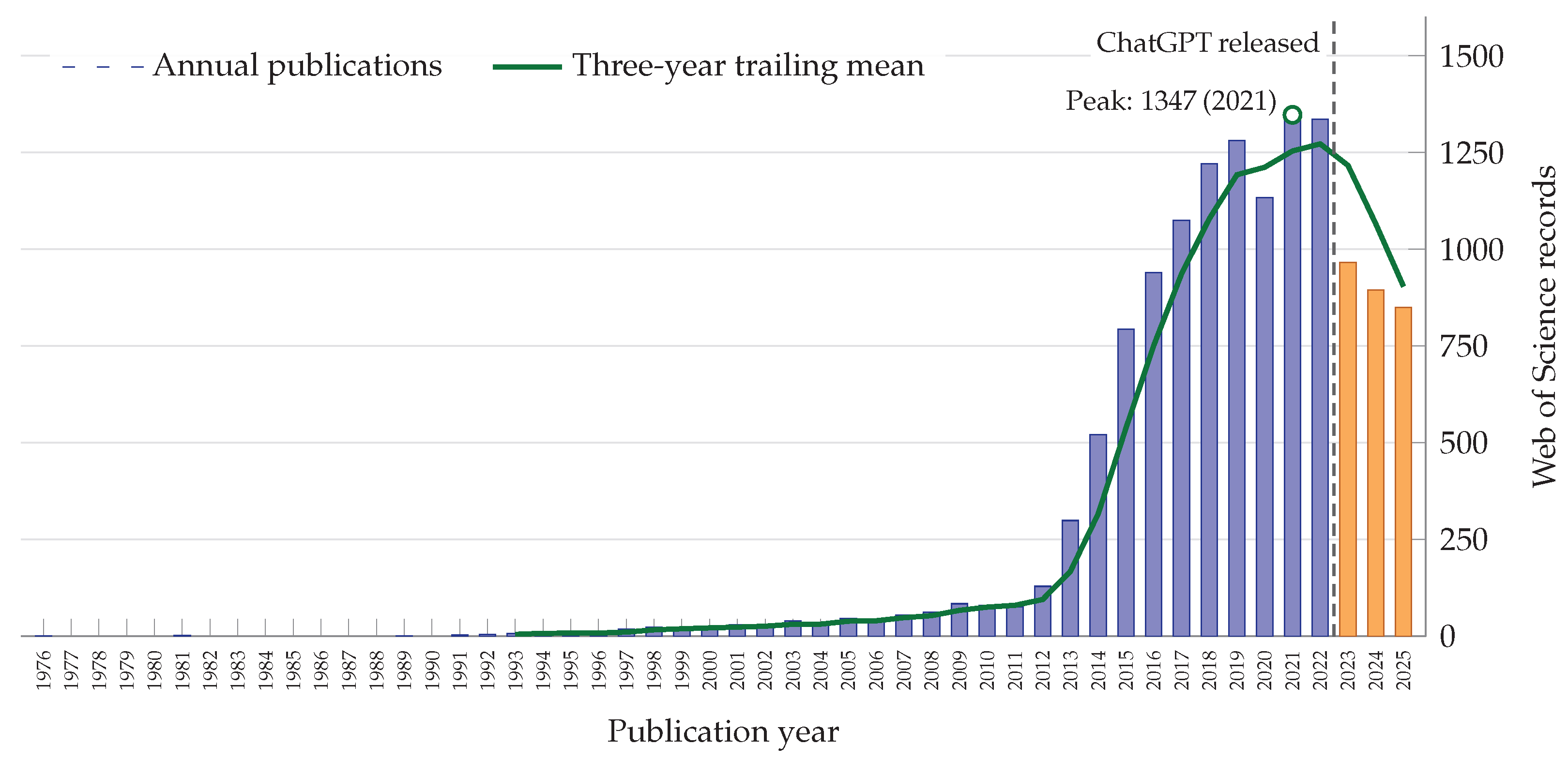
Web of Science records matching the Topic query for “big data clustering” show a marked long-term rise in research attention (Figure 1). Annual output increased from 80 records in 2010 to 1336 in 2022, reaching a peak of 1347 in 2021. Although the count subsequently declined to 850 in 2025, it remained more than ten times its 2010 level. The post-2022 decrease coincides with the public release of ChatGPT and the rapid expansion of research on large language models [15], and may partly reflect a shift in research terminology and attention toward generative AI. The sustained publication volume and evolving research focus reinforce the need for a structured review of scalable clustering methods.

Cluster analysis encompasses various models, among which the minimum sum-of-squares clustering (MSSC) is foundational and widely examined [16]. This model addresses the challenge of determining k centroids $C=\left(c_1,\dots ,c_k\right)\in {\mathbb{R}}^{n\times k}$ from m data points $X=\{x_1,\dots ,x_m\}$ within Euclidean space ${\mathbb{R}}^n$. The goal is to minimize the sum of squared Euclidean distances between each point $x_i$ and the nearest centroid $c_j$, as articulated in the equation:

$$\underset{C}{min}f\left(C,X\right)={\displaystyle \sum _{i=1}^m}\underset{j=1,\dots ,k}{min}{\parallel x_i-c_j\parallel }^2$$

(1)

where $\parallel ·\parallel$ denotes the Euclidean norm. This Equation (1) represents the objective function, or the sum-of-squared distances, determining the quality of a partition $X=X_1\cup \dots \cup X_k$ by how tightly data points are assigned to their closest centroids $c_j$. For arbitrary k and m values, the main challenge of producing high-quality solutions to the MSSC problem lies in its NP-hard nature [16], while big data contexts aggravate this problem much further.

In this review, big-data conditions refer primarily to a large number of objects m, rather than a large number of features n or clusters k. Methods developed specifically for high-dimensional or large-k regimes are therefore outside the review scope. Although Euclidean distance can become less discriminative in high dimensions because of distance concentration [17], this behavior depends on the data representation and does not imply that MSSC categorically fails for every high-dimensional dataset.

The K-means algorithm (Lloyd’s algorithm [18]) is one of the simplest and most efficient clustering algorithms, which naturally minimizes the MSSC criterion (1). It can be considered a classic method for solving the MSSC problem [19]. When applied to small or large data, K-means can find high-quality local solutions in reasonable time [20]. Accordingly, many scalable MSSC methods are formulated as enhancements, accelerations, or higher-level uses of K-means. This paper treats such K-means-based methods as a central part of big data MSSC, while also considering other MSSC-oriented approaches whose mathematical logic remains tied to minimizing or approximating the sum of squared distances.

Accordingly, throughout this article, the term “K-means clustering problem” is used as applied shorthand for the MSSC optimization problem in Equation (1), consistent with established usage in the machine-learning and optimization literature [21,22], whereas the term “K-means algorithm” refers specifically to Lloyd’s alternating assignment–update heuristic. The broader solvers considered in the review and benchmark need not be literal modifications of Lloyd’s algorithm: they are included because they seek fixed-k centroid solutions under the same sum-of-squared-distances objective, and many of them additionally use K-means for initialization, local refinement, or solution improvement.

While K-means offers a fast local search within the solution space of the MSSC problem, it is not directly applicable to big data due to its time complexity of $\mathcal{O}(m·n·k)$. Making a full pass through the dataset is necessary for K-means, which becomes prohibitive under big data conditions. However, K-means is highly adaptable, allowing optimization at nearly every step for big data processing and offering flexible integration with advanced clustering metaheuristics. Moreover, K-means can still be effectively utilized to accelerate other clustering models, such as density-based clustering [23] and spectral clustering [24]. For a more detailed discussion on K-means, its steps, and opportunities for their optimization, we refer the reader to Section 3.

An additional structural feature of MSSC is the inherent cluster-label permutation symmetry of its objective, while its squared-Euclidean structure is invariant under translations, rotations, and reflections of the data space. Although an algorithm typically represents a solution as an ordered vector of centroids $C=(c_1,\dots ,c_k)$, the clustering and its objective value are unchanged under any permutation of these centroids. This creates multiple equivalent representations of the same solution and has practical consequences for global optimization, population-based search, solution matching, and the comparison of clustering results. The reviewed algorithms differ in whether they preserve these structures, exploit them through matching or set-based operations, or break them through initialization and incremental construction.

Viewed as a global optimization problem, MSSC aims to divide a dataset into clusters, optimizing a single objective detailed in (1) that inherently enhances within-cluster similarity and between-cluster dissimilarity. This optimization criterion is fundamental in assessing the performance of clustering algorithms, with global minimizers offering a more precise reflection of a dataset’s inherent clustering structure [25]. However, the search for global minimizers is hindered by the objective function’s significant nonconvexity, making MSSC a complex yet crucial problem in cluster analysis. The nonconvex landscape of the MSSC objective function becomes dramatically more complex as the number of data points increases, which is especially characteristic to big data conditions.

To address these MSSC challenges, which are exacerbated by big data contexts, several approaches have been proposed in the literature to explore the solution space and locate global minimizers which include, but are not limited to: gradient-based optimization techniques [26], stochastic optimization algorithms [2], metaheuristic search strategies [25,27], and hybrid approaches [28]. Gradient-based techniques [26] have a focus on providing a fast convergence to local minimizers but may get trapped in poor solutions due to the nonconvex nature of the objective function. On the other hand, stochastic optimization algorithms [2] incorporate randomness in the search process to escape local minima and explore a broader solution space. Metaheuristic search strategies [25,27] aim to balance exploration and exploitation in the search process. Hybrid approaches [28] are frequently used, as they can combine multiple different methods with the goal of not only leveraging their advantages but also acquiring new qualitative properties.

Despite the proposition of these numerous optimization techniques aimed at overcoming the high nonconvexity challenge of MSSC, each method presents its unique advantages and limitations, indicating the absence of a universally applicable solution, especially in big data environments. Consequently, this underscores the need for continued investigation to devise methodologies that are both more effective and resilient in identifying global minimizers, particularly within the intersection of the MSSC area with the expansive field of big data.

This review examines optimization approaches for big-data K-means clustering under the MSSC objective and compares their trade-offs in clustering quality, computational time, and algorithmic simplicity. Within the review, we consider both end-to-end MSSC algorithms and auxiliary MSSC-oriented techniques, including preprocessing, initialization, sampling, data summarization, memory-efficient representations, and acceleration strategies. K-means receives special attention because it is the fundamental heuristic for MSSC and serves as the core routine or refinement step in many scalable MSSC algorithms. For the experimental evaluation and LIMA-dominance analysis, we compare algorithms that produce a final clustering solution for a prescribed number of clusters k and whose core logic is directly based on minimizing or approximating the MSSC objective in Equation (1). Auxiliary techniques whose use depends on an additional adaptation layer or a downstream MSSC algorithm are reviewed as practically relevant methods, but are not benchmarked separately.

In today’s landscape, selecting the right clustering paradigm and tool for new big datasets is not a straightforward endeavor for practitioners. Without proper guidance, comprehending the strengths and constraints of existing clustering models within big data scenarios becomes challenging. Additionally, gaining insights into the range of appropriate big data clustering algorithms tailored for the specific dataset can prove to be daunting.

In this review, the surveyed methods are categorized into distinct groups. For each category, we explore the advanced algorithms it encompasses and evaluate the strengths and limitations of the corresponding approaches. We also conduct a comprehensive experimental analysis of selected MSSC algorithms. In this analysis, we adopt the dominance relation based on the “less is more” approach (LIMA) [29] as the principal criterion for comparing the algorithms. To the best of our knowledge, this study represents the first use of this criterion for evaluating big data clustering algorithms.

The LIMA dominance criterion, as established by Brimberg et al. [29], defines a comparative relation among a collection of algorithms. Specifically, it asserts that an algorithm is considered superior to another if it achieves equal or better performance in terms of average accuracy, execution speed, and simplicity, with strict improvement in at least one of these dimensions. In this paper, simplicity is quantified reproducibly by the filtered lexical-token count of an implementation in a fixed reference language. The aspect of simplicity becomes critical in the context of big data. A comprehensive discussion on the LIMA dominance criterion is provided in Section 5.

This article proposes evidence-based practical recommendations and a decision guide intended to assist in selecting MSSC algorithms for big data. We have also undertaken an extensive evaluation of selected MSSC algorithms for big data, available from the recent literature, using a large array of real-world datasets. These aspects of the current work distinguish it from our previous paper [2] that introduced the Big-means clustering algorithm. Moreover, the differentiation stems from the fact that in [2], we aimed to juxtapose Big-means with a sophisticated state-of-the-art heuristic, LMBM-Clust [26], alongside other relatively elementary standard algorithms. Conversely, in the current study, our objective is to conduct a structured survey and comparison of a diverse set of existing approaches for optimizing MSSC in the context of big data.

Earlier surveys establish the broader context for scalable clustering. Mahdi et al. [30] reviewed 101 scalable algorithms and emphasized the prevalence of complex implementations and cloud-oriented deployment. Other surveys observed that relatively few methods address the variety and velocity dimensions of big data [31,32], while Mohebi et al. [33] identified the continuing challenge of balancing clustering quality against the cost and overhead of parallel execution. The present review complements this literature by focusing specifically on fixed-k MSSC, distinguishing end-to-end solvers from auxiliary optimization mechanisms, experimentally comparing representative algorithms under a common protocol, and incorporating implementation simplicity through the LIMA dominance criterion.

Our paper has the following outline. Section 2 describes the main challenges associated with the field of big data clustering. Section 3 discusses K-means in more detail and sets the stage for the subsequent sections. Section 4 analyzes techniques for optimizing MSSC algorithms in big data environments, including K-means-based methods and related auxiliary techniques. Section 5 presents the LIMA dominance criterion used for algorithm comparison. Section 6 reports the experimental evaluation and integrates its results with the LIMA numbers. Section 7 translates the review and experimental findings into practical guidance for selecting and validating big data MSSC algorithms. Finally, Section 8 summarizes the conclusions and outlines future research directions.

Literature Search and Selection

The literature search was conducted in the Web of Science Core Collection and Scopus. We searched all fields using the keyword pairs “big data” and “clustering”, “large data” and “clustering”, “large-scale data” and “clustering”, “tall data” and “clustering”, and “massive data” and “clustering”. For each query, the resulting records were considered under three alternative orderings: highest citation count first, most recent publications first, and highest journal impact factor first. The resulting publication lists were then screened manually for methods relevant to MSSC under big-data conditions driven primarily by a large number of objects. Methods designed specifically for other scaling regimes, such as high-dimensional data or a very large number of clusters, were outside the scope of the review. The broader Web of Science query underlying Figure 1 was used to illustrate publication activity in big-data clustering and was not the sole query used to select the reviewed literature.

2. Problem Challenges

Big data clustering is a complex task that faces several challenges that can be grouped into a few categories. One of these categories is related to the computational and practical aspects of clustering algorithms, such as scalability [34], computational complexity [30], simplicity [35], as well as ease of implementation and parallelization [36].

The second category is concerned with the selection and application of clustering algorithms. Choosing an appropriate clustering algorithm and its parameters is crucial for effective data analysis, as different data types may require unique clustering methods. With the variety present in big data, it is particularly important to choose suitable clustering techniques to ensure successful insights.

The last category involves specific computational requirements and limitations, such as computational resources [37], storage and retrieval [38], time-dependency, and real-time analysis [39].

Scalability can be defined as the ability to find the balance between the quality of the obtained solution and the amount of processed information (computational cost) in response to changes in volume and configuration of input data [2]. Traditional clustering algorithms that work well with small and large datasets may not be suitable for big data due to its increased computational complexity and memory requirements. Additionally, big data is often stored across multiple machines and storage systems, making it challenging to perform clustering analysis efficiently. To handle big data, clustering algorithms need to be designed to utilize distributed computing architectures and parallel processing [34].

The computational complexity of traditional clustering algorithms can make analyzing big datasets difficult within a reasonable amount of time. This is especially true when there is a need for real-time or near-real-time analysis. As noted by Mahdi et al. [30], the time required to perform clustering on large datasets can be prohibitive.

Modern clustering algorithms increasingly combine several optimization mechanisms. Such hybridization can improve solution quality, but it also increases runtime, memory use, parameter-tuning effort, implementation difficulty, and deployment cost, particularly on parallel or distributed architectures [35]. Researchers should therefore not treat increasing algorithmic complexity as an objective in itself or simply pursue progressively more elaborate hybrid methods. When proposing a complex method, they should also investigate whether comparable or better effectiveness and efficiency can be attained by a simpler algorithm under the same evaluation protocol. This motivates treating simplicity as an explicit comparison dimension alongside accuracy and speed.

Parallelizability is essential in the context of clustering algorithms as it refers to an algorithm’s capability to decompose the initial, large task into multiple smaller subtasks. This decomposition enables the concurrent (parallel) and independent processing of these subtasks by several processors or workers, shortening the overall processing time. The final solution to the original task is then derived by integrating the solutions of these smaller subtasks. Parallelization enhances an algorithm’s efficiency and scalability by effectively decomposing tasks and enabling parallel processing, while also optimizing the use of available computing resources and speeding up data processing. As noted by Alguliyev et al. [36], this is a crucial consideration for any clustering algorithm, particularly those designed to handle big datasets.

Choosing the right clustering algorithm and its parameters is essential for each dataset. There are various clustering algorithms available, each with its own unique strengths and weaknesses. However, selecting the most suitable algorithm for a specific dataset can be challenging, particularly when dealing with large datasets. Different algorithms may have varying computational requirements, and some may not be scalable to large datasets. Furthermore, most advanced clustering algorithms involve a large number of hyperparameters but do not provide clear guidelines for their optimal selection. Performing an ordinary grid search may be unfeasible in big data conditions due to unacceptable time costs. Although hybrid methods can improve solution quality, the need to optimize a large number of hyperparameters can impede their reproducibility and widespread adoption.

Clustering big data can require substantial computational resources, including processing power, memory, and storage [37]. Thus, to perform clustering analysis on big data, organizations may need to employ high-performance computing (HPC) technologies, including investing in specialized hardware or cloud computing services.

Storing and retrieving large datasets can present a challenge, particularly when real-time or near-real-time analysis is required. Big data clustering may necessitate specialized distributed storage and retrieval systems capable of handling large data volumes and providing quick access to data for analysis [38]. Furthermore, some big datasets may be too large to fit into the RAM of a computing system.

Some big datasets may have a time-dependent nature, so the patterns and relationships in the data may change over time [39]. Clustering algorithms may need to be adjusted to handle the time-dependency of the data and ensure that the clustering results remain relevant. Real-time or near-real-time clustering of big data can be challenging because of the need for fast processing and the large volume of data. Developing real-time clustering algorithms that can handle big data is an active area of research [39].

To summarize, all the above points show that the emergence of big data entails a set of unique challenges. To extract insights and value from vast datasets, there is a need for specialized clustering techniques (“true big data” algorithms [2]). These algorithms are specifically designed to address the big data issues and the inadequacy of classic approaches. This remains an active area of research. In this paper, we review the numerous attempts made in the literature to create big data clustering algorithms.

3. K-Means Algorithm

Partitioning-based clustering methods, especially K-means [18], excel in big data analysis by creating non-overlapping subsets where each data point is associated with a single cluster. These methods, which also include K-medoids [40] and CLARA [41], are efficient and scalable, making them ideal for handling large datasets. They start with initial centroids and refine these through iterative optimization to reduce within-cluster variance. Despite the necessity to predetermine the number of clusters and their sensitivity to initial centroid placements, partitioning-based algorithms remain central to big data clustering tasks. For this reason, this study concentrates on MSSC methods whose objective is explicitly tied to centroid-based minimization of within-cluster squared Euclidean distances.

As highlighted in the introduction, K-means is regarded as one of the most popular methods for addressing the MSSC problem. Its popularity stems from the method’s relatively high effectiveness, coupled with its simplicity and versatility. A pseudocode for the K-means algorithm is provided in Algorithm 1.

Algorithm 1: K-means

K-means is an iterative algorithm consisting of two alternating steps: assignment and update. The algorithm’s input is an initial set of k centroids $C=\left(c_1,\dots ,c_k\right)$ and some stopping criterion, which can be a maximum number of iterations or a tolerance on the distance between two consecutive solutions. In the assignment step, each point $x_i$ is assigned to the nearest centroid from C. In the update step, the centroids are updated by assigning the means of points in each cell $X_j$ of the resulting partition: $c_j={\displaystyle \frac{1}{\left|X_j\right|}}{\sum }_{x_i\in X_j}{x}_i$. These two steps are repeated until the stopping criterion is met.

Due to its simple and straightforward structure, K-means is amenable to optimization at nearly every stage in general and specifically for big data. First, before running the K-means algorithm, it might be advisable to perform normalization or dimensionality reduction on the input data. Second, the choice of initial centroids is an important part of the K-means algorithm, which significantly impacts the accuracy of the resulting clustering solution [42]. The classical version of K-means algorithm initially assigns centroids to clusters using a uniform random initialization. However, it has been established that the clustering solution obtained with a random initialization of K-means may be significantly worse in terms of the objective function when compared to the optimal clustering solution. This means that relying solely on random initialization can lead to suboptimal clustering results [43]. Therefore, improving initialization is another method for optimizing the performance of K-means.

The initialization issue of the classical K-means algorithm can be addressed through two main approaches. The first one involves selecting the initial solution carefully, as suggested by Franti et al. [42] and Ismkhan et al. [44]. The other approach is embedding the K-means algorithm into a global optimization method as a local search procedure, as proposed by Franti et al. [42]. Thus, numerous search methods, both local [27] and global [28], have been proposed to offer improved solutions.

One of the most effective heuristics for K-means initialization is K-means++ [21]. K-means++ works as follows: the first cluster center $c_1$ is chosen randomly from all data points. Each subsequent cluster center $c_j$ is selected from the remaining data points with a probability proportional to its squared distance from the existing cluster centers. The pseudocode of K-means++ can be found in Algorithm 2. While K-means++ initialization takes longer than a random initialization, it ensures that K-means requires fewer iterations to reach an optimum. Additionally, K-means++ often produces a smaller objective function value at the final solution compared to a naive random initialization. In [45], Makarychev et al. demonstrated that the expected cost of the solution produced by K-means++ is at most $5(logk+2)$ times the optimal solution’s cost. In the meantime, the time complexity of the K-means++ initialization is $\mathcal{O}(m·n·k)$. Hence, it is also not directly applicable to big data. However, the K-means++ algorithm can be efficiently parallelized for multicore processing of large data. In K-means and K-means++, parallelization can be used to compute the distances between centers and data points. In K-means++, it is also possible to parallelize the computation of the probabilities for selecting each data point as a center.

Algorithm 2: K-means++ initialization

A simpler but less efficient initialization method is Forgy [46], which also samples an initial solution from the original data points, but uniformly at random. Multistart K-means [42] is yet another initialization method, which executes several random initializations and picks the best one in the end.

The main loop of the K-means algorithm can be parallelized both in a parallel multistart manner and at the level of internal parallelization within each iteration, especially during distance calculations in the assignment step. The same distance calculation step can also be optimized using the triangle inequality [47,48].

During the operation of the K-means algorithm, various “divide and conquer” techniques can also be applied, where initially the data are divided and distributed among parallel workers, solutions for small subtasks are obtained, which are then combined at the final stage to produce a solution for the entire task. Decomposition of input data into subtasks can be accomplished in multiple ways, such as simple uniformly random sampling [2] or more advanced summarization techniques [49,50]. In this review, these techniques are discussed as MSSC-oriented auxiliary mechanisms; their experimental role depends on the downstream clustering algorithm in which they are embedded.

During the parallelization process, advanced optimization methods can also be employed, such as collective or genetic algorithms, among others. In this approach, K-means is integrated as a local search procedure within higher-level heuristics such as MDEClust [28], HG-means [25], or Big-means [2]. K-means can be optimized by using High-Performance Computing (HPC) technologies such as vector computations based on SIMD technology and others implemented in Numba [51,52], among others.

4. Optimization Approaches for Big Data K-Means Clustering

The literature proposes numerous techniques to improve MSSC scalability and solution quality in big data contexts. Since K-means is the foundational heuristic for MSSC, many of these techniques are formulated as modifications, accelerations, or extensions of K-means. In this section, we review these techniques and classify them into separate categories. For each category, we consider representative algorithms and analyze their strengths, weaknesses, and role in big data MSSC.

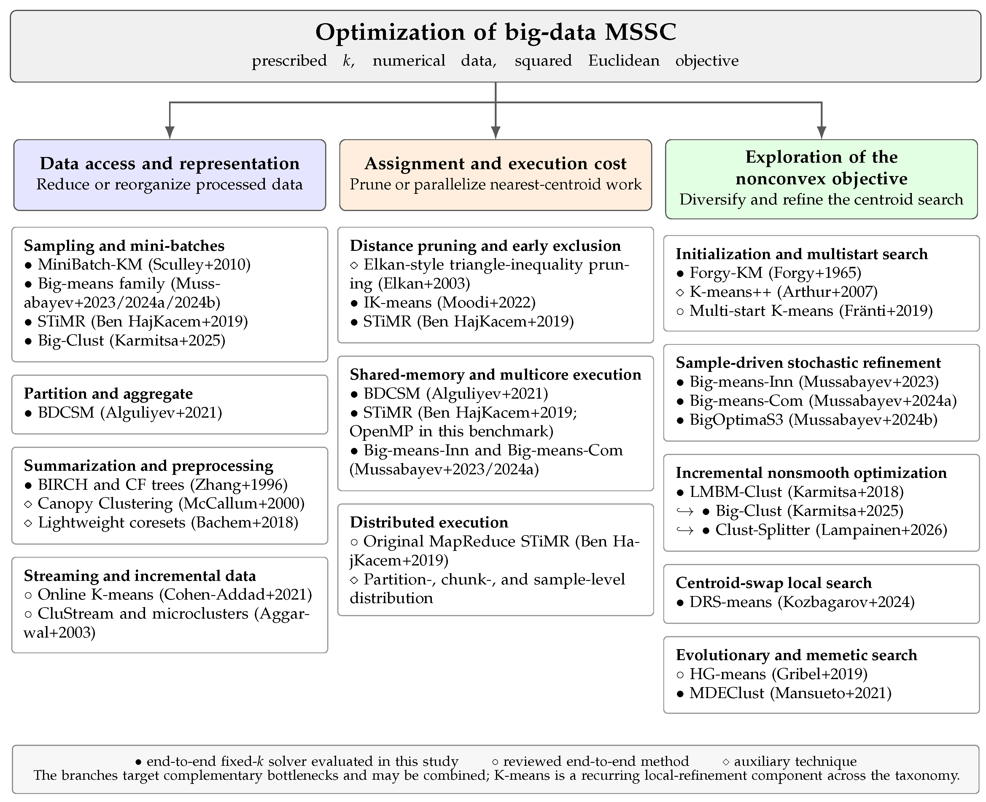
Figure 2 organizes the reviewed literature by the part of the MSSC computation that each method primarily changes: data access and representation, assignment and execution cost, or exploration of the nonconvex objective. These mechanisms are composable rather than mutually exclusive. For example, STiMR combines sampling, distance pruning, and parallel execution; Big-Clust combines sampling with nonsmooth optimization; and the Big-means variants combine sample-based refinement with parallel execution. The symbols in the figure also distinguish end-to-end fixed-k solvers from auxiliary techniques and identify which solvers enter the common experimental evaluation.

The data-access and representation branch contains methods that reduce, summarize, partition, or incrementally process the data presented to the clustering procedure, thereby limiting repeated access to the full dataset. The assignment and execution-cost branch targets the computational expense of assigning objects to their nearest centroids through distance pruning, shared-memory parallelism, or distributed execution. The nonconvex-objective branch instead targets the quality of the centroid search through initialization, multistart strategies, stochastic refinement, nonsmooth optimization, centroid swaps, and evolutionary or memetic search. The three branches therefore identify complementary computational bottlenecks rather than mutually exclusive classes of algorithms.

4.1. Data Decomposition

This approach involves partitioning the data into smaller subsets and performing clustering on each subset independently. The clustering of each subset can be considered as a separate subproblem. When all the subproblems have been solved, their solutions are combined to form a solution for the original problem.

Decomposition can be performed in different ways:

• Partitioning. This can be achieved using techniques such as vertical partitioning or horizontal partitioning. In vertical partitioning, the data is partitioned based on the features, whereas in horizontal partitioning, the data is partitioned based on the instances. This approach can be effective when the data is too large to fit into memory or when the computation time is a bottleneck;
• Sampling. This approach involves selecting a random subset of the data and clustering it. The resulting clusters can then be used as an approximation of the clusters that would be obtained from clustering the entire dataset. This approach can be effective when the data is uniformly distributed and the clusters are well separated;
• Stream-based clustering. This approach is also called the online or incremental clustering. It involves clustering data points in small batches in real-time as they arrive, without needing to store the entire dataset in memory. Thus, clusters are updated as new batches arrive. This approach can be effective when the data is continuously streaming, and real-time clustering is required (the clusters need to be updated dynamically).

All three decomposition methods are tightly interrelated. Each method can be naturally transformed into another one.

The MSSC objective is invariant to data ordering, whereas deterministic partitioning or streaming order can introduce computational asymmetry.

Minibatch K-means [53] is a basic algorithm that utilizes the sampling approach. In each iteration of the MiniBatch K-means algorithm, a minibatch (a random subset of the data) is selected for processing. Then this minibatch goes through the assignment and update steps, as in the standard K-means. However, rather than updating each centroid by averaging all data points assigned to it, the update is made using a fraction of the points in the minibatch. Specifically, the new centroid position is a weighted average between its old position and the mean of the new points assigned to it. The weights ensure more recent data has a larger influence on the centroid position, allowing the algorithm to better adapt to changes in the data distribution.

The algorithm continues to iterate, selecting new minibatches and repeating the assignment and update steps, until a stopping criterion is met. This could be a fixed number of iterations, or a point where the centroids no longer move significantly between iterations.

Thus, the Minibatch K-means algorithm consists of the following key steps:

• Initialization. Randomly select k points from the dataset to act as the initial cluster centroids;
• Sampling. Draw a random minibatch M of size b from the dataset;
• Assignment. Assign each data point in the minibatch to its nearest centroid;
• Update. Update the affected centroids using the minibatch points assigned to them;
• Repeat. Repeat steps 2–4 until the centroids no longer move significantly.

The pseudocode for the Minibatch K-means algorithm is shown in Algorithm 3.

Algorithm 3: Mini-batch K-means

    In each iteration of Minibatch K-means, the centroids are updated only using the points of an incoming minibatch, making the algorithm more memory-efficient and scalable than traditional K-means. However, the quality of the solution may be drastically affected by the randomness of the minibatch selection, and lots of random initializations may be required to obtain an optimal result. The Big-means algorithm [2] addresses these limitations by implementing a stable and effective K-means++ initialization for the initial sampled subset and degenerate clusters. It also introduces an advanced centroid update criterion based on the optimal objective function value obtained from all processed samples. Furthermore, Big-means deepens the exploration of each new sample by employing a K-means local search strategy. All these modifications significantly enhance the stability and precision of the clustering outcomes [2].

The Big-means algorithm represents a synthesis of three key approaches to data decomposition. This simple method begins by sampling a subset S from the dataset X, containing s data points, a small fraction of the total m. It leverages the K-means++ algorithm for the initial selection of centroids C from S. Subsequently, it employs a dynamic clustering process, utilizing K-means with the most effective centroid set found across previous samples. This iterative refinement, guided by the “keep the best” strategy, continually updates to the incumbent solution, based on the sum-of-squares criterion evaluated on current samples. Algorithm 4 encapsulates the Big-means algorithm.

Unique to Big-means is its strategy for handling empty clusters: it rejuvenates these by reapplying K-means++ to produce new potential centers, thus avoiding the pitfalls of traditional methods and enhancing the solution’s quality by broadening the search for minimizing the objective function. Another pivotal feature of Big-means is the “shaking procedure”, which generates new samples to perturb the current centroid solution, thereby infusing diversity and adaptability into the clustering process. By treating the dataset as a point cloud in the n-dimensional space, each sample acts as a sparse representation, injecting fresh perspectives into each iteration.

Upon reaching a predetermined time limit or processed sample count, Big-means assigns all data points to the best obtained centroid configuration C. However, this step can be either omitted or adjusted according to the specific requirements of an application area. The algorithm’s iteration time complexity stands at $\mathcal{O}(s·n·k)$, offering a significant speed advantage for big datasets, especially when compared to the conventional K-means or K-means++ algorithms.

Alguliyev et al. took a different approach in their Big Data Clustering on a Single Machine (BDCSM) algorithm in [36]. BDCSM partitions large datasets into chunks, clusters them in parallel using K-means, and aggregates the resulting cluster centers into a final pool. Then, the algorithm clusters the pool using K-means. The pseudocode for the BDCSM algorithm is presented in Algorithm 5. BDCSM is a prominent instance of partition-based parallel clustering algorithms. While BDCSM is a straightforward algorithm that leverages parallel processing to accelerate clustering and partially addresses the challenge of distributed storage for big data, it fails to address the initialization issue, resulting in reduced clustering accuracy (effectiveness) despite its gains in efficiency.

Algorithm 4: Big-means

The empirical evaluation of BDCSM in the original paper showed its superiority over the classical K-means algorithm [36]. However, this evaluation did not demonstrate any superiority of BDCSM to other more advanced algorithms for clustering large datasets.

Algorithm 5: BDCSM

Notable examples of online clustering algorithms include online K-means [59] and online spectral clustering [63]. Online K-means updates the cluster centroids incrementally as each new data point arrives, without the need to access the entire dataset. After initializing k centroids, each incoming point is assigned to its nearest centroid; the corresponding centroid is then updated using a running average based on the number of points assigned to it so far. This gives the Online K-means algorithm an advantage over traditional K-means in terms of processing real-time data and scalability to large datasets. However, it still shares several limitations with Minibatch K-means and BDCSM, including centroid initialization issues, convergence to local optima, and ignoring degenerate clusters. Furthermore, Online K-means processes observations sequentially rather than as complete chunks, making the final clustering outcome highly sensitive to the order of incoming data points.

With sufficient computational resources, data decomposition enables the application of advanced parallel and distributed techniques to individual subproblems, as explored in the next subsection, unlocking vast opportunities for more efficient processing and analysis.

4.2. Parallelization and Distributed Computing

Parallelization and distributed computing are two common techniques for optimizing MSSC methods in big data settings [36]. Most commonly, parallelization involves breaking the data into smaller subsets and clustering them simultaneously on multiple processors. The results are then combined to generate the final clusters. This approach can be useful when the data is too large to fit into memory or when the computation time is a bottleneck. Alternatively, big data can be distributed across multiple machines. In this case, clustering is performed in a distributed manner, using frameworks such as Apache Hadoop or Apache Spark. This approach can be effective when the data is too large to fit on a single machine. By distributing the data and computations, the workload can be divided among multiple machines, reducing the processing time and allowing for scalability.

Ben HajKacem et al. [56] proposed STiMR K-means, where STiMR stands for Sampling, Triangle inequality, and MapReduce. The method first draws a random sample from the input dataset, then applies K-means to this sample while using the triangle inequality to reduce unnecessary distance computations, and finally assigns all original data points to the obtained centroids. In the original formulation, these stages are implemented as three MapReduce jobs: data sampling, data clustering, and data assignment.

In our experimental evaluation, STiMR is included through a C++ implementation parallelized with OpenMP. This implementation preserves the main algorithmic ingredients of STiMR while replacing the MapReduce execution layer by shared-memory parallel loops and reductions. For datasets that fit into a single system’s RAM, this implementation is expected to have substantially lower execution latency than a Hadoop-style MapReduce implementation, since it avoids distributed-file-system writes, serialization, shuffling, and network communication. At the same time, the original MapReduce formulation remains relevant for deployments where data exceed the memory of a single machine or where distributed fault tolerance is required. Algorithm 6 summarizes the shared-memory version used in this study.

However, the logic of some other big data clustering algorithms allows for other types of parallelization. For instance, independent or somewhat dependent loops inside a clustering algorithm can be naturally parallelized. Big-means [2] is a good example that is amenable to this kind of parallelization. Specifically, each sample-processing iteration in Algorithm 4 can be assigned to a separate parallel worker. These workers can be totally independent from one another (competitive parallelization) or share information about the best sample solutions (collective parallelization) [54,64]. The former mode promotes exploration among the initial solutions, while the latter ensures a thorough exploitation of the best initial solution. Additionally, one can consider a hybrid parallelization mode, in which for some number of iterations the competitive mode is employed until being switched to the collective mode. The hybrid mode is expected to combine both benefits of the competitive and collective parallelization schemes, achieving an optimal trade-off between them.

BigOptimaS3 [55] extends competitive parallel Big-means by optimizing the sample size stochastically during execution. Each worker independently draws a sample size $s_w$ from an admissible interval $[s_{min},s_{max}]$ and performs p Big-means passes using that size. When a new $s_w$ is drawn, the worker’s incumbent objective is recalculated because objective values obtained from samples of different sizes are not directly comparable. Whenever a worker improves its incumbent solution, the corresponding $s_w$ is added to a shared list L. At termination, the empirical distribution of improving sample sizes is analyzed, and its mean is used as the expected improving size $s_{\mathrm{opt}}$. The worker incumbents are then compared on a common random sample of size $s_{\mathrm{opt}}$, after which the best centroid set is used to assign the full dataset. Thus, the method searches competitively over both centroid configurations and sample sizes, using the accumulated improvements to identify a sampling scale that balances computational sparsification against the representation of lower-density regions.

Algorithm 6: STiMR K-means with shared-memory parallelization

Throughout our experimental phase, we use shared-memory implementations for algorithms whose original logic can be expressed on a single machine. Earlier Python-based implementations relied on the Numba library [51,52] to parallelize the specific loops highlighted as parallelizable in the original papers. For STiMR, the experimental implementation is written in C++ with OpenMP, which is a more natural fit for its repeated assignment and reduction operations.

To maximize memory efficiency in MSSC clustering, the next subsection describes how algorithms may employ more frugal data structures to represent the dataset, which are then either directly passed to K-means for iterative refinement or in some other way adapted to yield an MSSC solution.

4.3. Memory-Efficient Algorithms

Memory-efficient clustering algorithms are designed to handle datasets that are too large to fit into memory. These algorithms typically take advantage of some form of data summarization, disk-based processing, or online updates to reduce the memory footprint. In the MSSC setting, such summarization is useful only when the resulting statistics can still support centroid-based assignments and the minimization of the sum of squared distances.

BIRCH (Balanced Iterative Reducing and Clustering using Hierarchies) [58] is a fundamental memory-efficient algorithm for large-scale centroid-based clustering. It builds a Clustering Feature (CF) tree whose entries store the number of points, linear sum, and squared sum of each subcluster. These statistics naturally support centroid-based distance measures and variance-increase criteria, aligning BIRCH with the MSSC framework when its default centroid-based metrics are used. Because branching decisions rely on centroids and radii, BIRCH also inherits the usual spherical-cluster assumption of MSSC methods. In its final phase, BIRCH can apply a partitional refinement step to the leaf entries of the CF tree, using their compact sufficient statistics to obtain a global centroid-based solution.

The main BIRCH procedure, adapted from the original four-phase description of Zhang et al. [58], is summarized in Algorithm 7. A CF entry is denoted by $(N,LS,SS)$, where N is the number of points in a subcluster, $LS={\sum }_i{x}_i$ is their linear sum, and $SS={\sum }_i{x}_i^{\top }{x}_i$ is the scalar sum of squared Euclidean norms.

CluStream [60] is an MSSC-related algorithm for evolving data streams. It maintains lightweight microclusters in real time and periodically applies K-means to obtain macroclusters. However, CluStream is not included in the static-data experiments of this paper. Forcing a static dataset into CluStream by reading it as an artificial stream ignores the algorithm’s temporal architecture. Its timestamp statistics, decay mechanisms, and pyramidal time frame are designed for evolving data rather than unordered static datasets. Such a conversion would introduce arbitrary ordering sensitivity and lossy summarization while offering no natural way to define meaningful time-spaced observations.

4.4. Preprocessing and Data-Reduction Techniques

Several preprocessing and data-reduction techniques are highly relevant to big data MSSC, even though their practical use depends on a downstream clustering algorithm. Canopy Clustering [50] first forms coarse, possibly overlapping groups of points using a computationally cheap distance measure and two thresholds $T_1>T_2$. A selected point starts a new canopy; points within the loose threshold $T_1$ are assigned to that canopy, while points within the tighter threshold $T_2$ are removed from the pool of future canopy centers. The resulting canopies can then be used to reduce the candidate comparisons or initialize a downstream clustering method. The lightweight coreset framework [49], in turn, constructs a small weighted subset of the original data for downstream MSSC optimization. It computes the data mean, samples points according to a mixture of uniform probability and squared distance from the mean, and assigns inverse-probability weights so that the weighted subset approximates the full-data MSSC objective. These methods are excluded from the experimental evaluation because their final clustering quality depends heavily on the downstream algorithm applied after preprocessing. Moreover, Canopy Clustering requires choosing the thresholds $T_1$ and $T_2$, whereas lightweight coresets require an appropriate coreset size. These extra parameter-selection problems introduce additional overhead in big data settings and usually require dedicated heuristics.

Algorithm 7: BIRCH

Beyond hardware acceleration and memory efficiency, K-means optimization can be achieved through analytical refinement of the underlying mathematical operations, as explored in the next subsection.

4.5. Triangle Inequality

During K-means clustering, it can be observed that not all points alter their cluster membership. By using some logic to identify and label these points as fixed, the algorithm can avoid the need to recalculate cluster distances for them. This optimization can significantly reduce computation time. The triangle inequality is widely employed to identify points that remain fixed to their respective centroids across iterations [47].

Moodi et al. introduced an optimized version of the K-means algorithm that utilizes the triangle inequality to reduce processing time [48]. Their approach applies the A-means algorithm according to Early Classification (EC), which stabilizes points to their respective clusters based on the probability of membership change in subsequent iterations. This reduces the computational time required for assigning points to clusters, especially for large datasets. However, significant movement of centroids in some iteration can lead to inaccurate results. To address this issue, the authors proposed a method to reintroduce stabilized points into computation if their distances from the centroids exceed the cluster radius. This ensures that the approach achieves significant computational savings without compromising accuracy. We have included this algorithm into our experiments under the name IK-means. The pseudocode of the IK-means algorithm is shown in Algorithm 8.

Algorithm 8: IK-means

The IK-means algorithm reduces the computation of the K-means algorithm by reducing the number of points that need to be reassigned to clusters in each iteration. This is achieved by introducing the concept of exclusion, where points that are very likely to remain in their current cluster are excluded from further consideration in the algorithm. The exclusion is based on the triangle inequality, which can help estimate whether a point is likely to change its cluster assignment or not, thus reducing the number of distance computations in the algorithm.

The triangle inequality can also be leveraged to accelerate the K-means local search within the Big-means algorithm, resulting in a substantial increase in efficiency.

The following subsection explores another avenue for optimizing K-means: improving initialization efficiency through strategic sampling.

4.6. Sampling-Based Initialization

Initializing the K-means algorithm on a small random subset of the data and then applying it to the entire dataset is a powerful strategy for optimizing K-means in the big data context. This approach addresses scalability challenges, enabling the use of more advanced initialization methods for improved clustering performance.

CluDataSE [65] is a hybrid of DBSCAN and the assignment logic of Lloyd’s algorithm and can be viewed as MSSC-related. It first draws a random sample of size $n/\mathit{sampleFactor}$ and applies DBSCAN, with $\epsilon$ derived from a minPts-distance graph and minPts scaled in proportion to the dataset size. The medoids of the DBSCAN clusters are then used as initial centroids, and the remaining data points are assigned to their nearest centroid, reducing the risks associated with randomly selected K-means representatives. CluDataSE subsequently applies a weighted splitting mechanism to sufficiently populated clusters: the point farthest from the current centroid and its reflection across that centroid initialize two candidate subclusters, and a split is retained only when the resulting clusters satisfy population and separation conditions. This step is intended to separate dense or nearly uniform regions that DBSCAN may merge into a single cluster. Nevertheless, CluDataSE is excluded from the experimental evaluation because it is not naturally compatible with the fixed-k benchmark protocol used in this paper. Its initial number of centers is determined by density parameters, while the splitting mechanism can further change the number of clusters; therefore, the final cluster count emerges from density and splitting criteria rather than being reliably prescribed by the user as a fixed MSSC parameter.

The multistart K-means algorithm [42] is a variant of the K-means algorithm that aims to improve the quality of the produced clusters by running the K-means algorithm multiple times with different initializations. The algorithm randomly initializes the cluster centers multiple times and runs the K-means algorithm on each initialization. The final set of clusters is selected from among the various runs based on the lowest sum of squared distances between the data points and their respective cluster centers.

The Forgy K-means algorithm [66] is a simple and efficient variant of the K-means algorithm. Unlike random initialization, where centroids are chosen as random locations in the space, Forgy initialization randomly selects k data points from the dataset to serve as the initial centroids. This approach ensures that the initial cluster centers are actual data points, making them more representative of the dataset and potentially leading to faster convergence of the algorithm. This selection strategy leads to the initial cluster centers that are more likely to be close to the true cluster centers since randomly picked data points tend to be close to regions with high density. Meanwhile, using random space locations can sometimes lead to initial centroids that are not representative of the dataset or that are too far away from the true clusters.

The Big-means algorithm exemplifies the use of K-means++ initialization on a random subsample of the dataset. The algorithm then employs an iterative process to improve the current best set of centroids using local search on various subsequent subsamples, thereby reducing the dependence of final results on the accuracy of initialization. As a result, different initialization schemes can also be used on the first sample in Big-means.

Another simple sampling method, employed by the Big-means algorithm, involves drawing a uniform random sample from the available data X. This approach has low computational overhead and does not require the construction of auxiliary probability distributions or density estimates. Under suitable assumptions on the dataset structure, uniform sampling can still produce representative subsets for MSSC optimization [67]. Its practical effectiveness, however, depends on the sample size and on how well the sample reflects the geometry of the full dataset.

The following subsections explore advanced MSSC optimization strategies that apply nonsmooth optimization directly to the MSSC objective, use randomized swap-based local search, or combine centroid-based local search with higher-level evolutionary mechanisms.

4.7. Nonsmooth Optimization Approaches

The MSSC objective in Equation (1) can also be viewed as a nonsmooth, nonconvex finite-sum optimization problem over the cluster centers alone. In this reduced view, assignments are not represented by explicit binary variables: for a centroid set $C=\{c_1,\dots ,c_k\}$, each point simply contributes its squared distance to the closest center. The nonsmoothness comes from this nearest-center choice, since the active closest center can change when a point crosses a Voronoi boundary. This representation is attractive for large-scale clustering because the number of continuous variables is $nk$, independent of the number of data points m, and no explicit assignment variables are introduced.

A bundle method is designed for precisely this type of nonsmooth objective. Instead of following a single gradient, it stores several past subgradients and function values, which together form a local piecewise-linear model of the objective. The limited memory bundle method (LMBM) keeps only a small amount of this information and combines it with a variable-metric approximation of curvature. Intuitively, each LMBM call alternates between constructing a search direction from the stored bundle, testing whether the trial point gives a sufficient objective decrease, and updating the bundle information. Successful trial points become serious steps; unsuccessful but informative trials still enrich the local model of the nonsmooth landscape.

Karmitsa et al. proposed LMBM-Clust in [26], an incremental nonsmooth optimization method for large MSSC problems. The method starts from the one-cluster solution and adds one center at a time until the prescribed number of clusters is reached. At each stage, an auxiliary clustering problem is used to generate promising starting points for the new center, and LMBM [68] is applied both to the auxiliary problem and to the resulting full MSSC problem. The auxiliary problem asks where an additional center would be useful given the current $(l-1)$-center solution; after this candidate is refined, the full l-center objective is optimized again so that all centers can move jointly. The starting-center generation follows the incremental strategy of Ordin and Bagirov [69]. LMBM-Clust can produce high-quality fixed-k MSSC solutions, although its full-data optimization steps and parameterization may become demanding on very large datasets. The original implementation of LMBM-Clust provided by the authors was unable to cluster a significant portion of large real-world datasets in our previous experimental evaluation due to out-of-memory errors [2].

The ordered centroid formulation contains equivalent copies of the same solution under centroid-label permutations; incremental center insertion implicitly chooses one representative and therefore breaks part of this representational symmetry.

Algorithm 9 summarizes the clustering-level logic of LMBM-Clust. The LMBM calls are shown explicitly as nonsmooth optimization steps: at each such step, the solver improves a center set for an objective whose active terms are determined by the current nearest-center assignments. Thus, the listing emphasizes both central ingredients of the clustering method: incremental center insertion and repeated bundle-based refinement.

Big-Clust [57] extends this line of work to big data by introducing a stochastic limited memory bundle algorithm (SLMBA). The method keeps the incremental structure of LMBM-Clust but applies the starting-point search and the nonsmooth local optimization on sampled data and mini-batches. SLMBA can be understood as a batch-wise version of LMBM: instead of evaluating the full finite sum at every solver step, it optimizes a batch objective, uses stochastic subgradients computed on the current mini-batch, and periodically refreshes the batch. Importantly, it does not discard all previous information when a new batch is selected; the limited-memory correction information is carried forward, so the solver can retain a rough sense of curvature and search history while reducing the cost of each objective and subgradient evaluation. If the batch is taken to be the full dataset, SLMBA essentially returns to the deterministic LMBM setting.

Algorithm 9: LMBM-Clust

Big-Clust therefore uses randomness at two levels: it first builds each incremental clustering stage on a sampled subset of the data, and then its SLMBA solver uses mini-batches within that subset to perform nonsmooth optimization. When the sample is taken as the full dataset, the method follows the same incremental objective on all available points; when a smaller sample is used, the final centers are obtained from the sampled optimization process and can then be applied to the full dataset by nearest-center assignment.

The main Big-Clust procedure is shown in Algorithm 10. The thresholds used by the original method control how many candidate centers are retained after the auxiliary search and how broadly the stochastic refinement is initialized.

Clust-Splitter [61] develops the same NSO-based incremental philosophy in a different direction. Instead of searching for a new center globally, the method identifies the current cluster with the largest contribution to the objective and splits this cluster through two auxiliary optimization problems. First, a starting-point auxiliary problem identifies a promising second center for the selected cluster. Then, a two-cluster auxiliary problem splits this cluster into two parts. The resulting two centers, together with the unchanged centers from the previous solution, define a starting point for the full l-cluster MSSC problem, which is again refined by LMBM. This produces an intuitive and computationally focused incremental strategy, especially suitable when only a moderate number of clusters is required.

Algorithm 11 presents Clust-Splitter at the level used in this review. It keeps the LMBM solver as a named optimization step while spelling out the cluster-selection and two-center split operations that distinguish Clust-Splitter from the earlier incremental NSO methods.

Algorithm 10: Big-Clust

Algorithm 11: Clust-Splitter

Overall, LMBM-Clust, Big-Clust, and Clust-Splitter form a coherent NSO-based line of MSSC algorithms. LMBM-Clust established the full-data incremental bundle-optimization approach, Big-Clust adapts it to larger datasets through stochastic sampling and mini-batch bundle optimization, and Clust-Splitter narrows the incremental search by splitting the cluster that currently contributes the most to the objective.

However, limited-memory storage does not eliminate the dependence on dataset size: each exact objective or subgradient evaluation still requires assigning all points to their nearest centroids, and line searches, null steps, and incremental cluster construction can multiply these full-data scans. Sampling in Big-Clust reduces this cost but may underrepresent small or sparse clusters and make retained optimization information less reliable across changing samples. Similarly, the greedy splitting strategy of Clust-Splitter can propagate an unsuitable early split, while full-data refinement partly restores the computational cost it seeks to avoid.

4.8. Random-Swap Local-Search Approaches

Random-swap methods constitute another family of MSSC heuristics. The basic random-swap idea starts from a locally optimized K-means solution, removes one current centroid, inserts a data point as a candidate new centroid, and then applies K-means refinement. If the refined solution improves the MSSC objective, it replaces the incumbent solution. Repeated swaps allow the method to escape poor local minima because a single replacement can destroy an unproductive Voronoi region and create a new one in a previously underrepresented part of the dataset.

Because random-swap methods operate on centroid sets, their swap and acceptance logic is naturally insensitive to label ordering.

Kozbagarov and Mussabayev proposed DRS-means [62], a distribution-guided variant of the random-swap strategy for MSSC. Instead of selecting both the removed centroid and the inserted data point uniformly at random, DRS-means uses two probability mechanisms. First, it assigns larger probability to close pairs of centroids, for example using masses proportional to $1/\parallel c_l-c_r\parallel$ for centroid pairs $(c_l,c_r)$, and then removes one centroid from the sampled pair. The intuition is that two nearby centroids are more likely to represent a redundant local allocation of centers. Second, after a centroid $c_j$ is removed, the algorithm chooses its replacement from the data using a product of two effects: dense points are favored through an inverse distance to the h-th nearest neighbor, while points far from the remaining centroids $C\setminus \left\{c_j\right\}$ are favored through their squared nearest-center distance. In compact form, if $d_h\left(x_i\right)$ is the distance from $x_i$ to its h-th nearest neighbor and $d(x_i,C\setminus \left\{c_j\right\})$ is its distance to the closest remaining centroid, the replacement probability is proportional to

$${\displaystyle \frac{1}{d_h\left(x_i\right)}}d{(x_i,C\setminus \left\{c_j\right\})}^2.$$

After each proposed swap, K-means is used as a local improvement procedure, and the candidate solution is accepted only when it decreases the MSSC objective.

This design keeps the method close to the classical K-means framework while adding a global exploration mechanism. The main computational cost comes from repeated K-means refinements, whereas the probability calculations guide the search toward more informative swaps. The main user-facing search-budget parameter is the number of swaps, while the neighborhood size used in the point-selection distribution can be fixed by the implementation. Since DRS-means returns a fixed number of centroids and directly optimizes the MSSC objective, it fits naturally into the benchmarked family of MSSC algorithms.

Algorithm 12 summarizes DRS-means at the level of the centroid-swap mechanism. The listing makes the two probability mechanisms visible while keeping the notation compact: one distribution identifies redundant centroids, and the other balances local data density with distance from the current reduced centroid set.

For big data, DRS-means may be limited by the cost of obtaining nearest-neighbor density information and by the repeated data-wide distance calculations and K-means refinements required for each swap. Its density- and distance-based probabilities may underrepresent sparse clusters or overemphasize outliers, respectively, depending on h, feature scaling, and dimensionality. Moreover, single-centroid improving swaps can stagnate when escaping a poor solution requires several coordinated changes.

Algorithm 12: DRS-means

4.9. Evolutionary and Memetic Approaches

Evolutionary and memetic clustering algorithms combine centroid-based local search with higher-level population mechanisms. In the MSSC setting, these methods typically use K-means as a refinement procedure and rely on genetic or differential-evolution operators to explore new initial centroid configurations. This combination can improve solution quality, but it may also increase computational cost because many candidate solutions must be repeatedly refined.

Gribel et al. proposed a hybrid genetic clustering algorithm called HG-means in [25], which combines the multistart K-means approach with genetic operations such as mutation, crossover, and selection to select new initial centroids. The algorithm was shown to produce high-quality clusters and to be faster than many existing algorithms, with the exception of LMBM-Clust. However, HG-means requires clustering the full dataset in every iteration, which makes the algorithm computationally demanding in big data settings.

Mansueto et al. [28] proposed a Memetic Differential Evolution Clustering (MDEClust) algorithm for the MSSC problem. The algorithm combines the global optimization framework of differential evolution with the local search procedure of K-means clustering. The MDEClust algorithm evolves a population of solutions through crossover, mutation, and local refinement via K-means. The algorithm ensures diversity and avoids premature convergence by employing an innovative crossover operation based on differential evolution and a roulette wheel selection in the mutation process. The MDEClust algorithm has been shown to be efficient in generating high-quality solutions, especially for datasets with a large number of clusters and high dimensionality. In the computational study of Mansueto et al. [28], MDEClust was shown to be superior to HG-means and to attain state-of-the-art performance. However, the algorithm’s performance can be sensitive to the choice of initial population and parameter settings, including population diversity tolerance, maximum number of iterations, crossover parameter, and mutation parameter. While MDEClust outperformed HG-means in terms of clustering accuracy, scalability remains a challenge as the computational effort increases significantly, especially when the mutation operator is used.

The pseudocode of the MDEClust framework used in this paper is shown in Algorithm 13. We use the exact matching variant, where cluster centers from different parent solutions are aligned by solving the corresponding assignment problem with the Hungarian algorithm. This matching step is a symmetry-handling mechanism rather than merely an implementation detail: centroid sets that differ only by a permutation represent the same clustering, but population-based vector operations require their centers to be aligned before they are combined. The mutation flag distinguishes the exact-matching variants without and with mutation, respectively.

Algorithm 13: MDEClust with exact matching

Evolutionary and memetic methods multiply the cost of full-data assignment and local search across a population and many generations; in MDEClust, centroid matching additionally becomes expensive as k grows. Candidate evaluations can be parallelized, but may remain constrained by memory bandwidth and repeated access to the dataset. Their scalability and runtime also depend strongly on population, variation, local-search, and stopping parameters, making direct application to streaming or out-of-core data difficult without potentially accuracy-reducing approximations.

In summary, evolutionary and memetic MSSC algorithms can be highly effective when solution quality is prioritized, but their repeated use of local search makes scalability a central concern. In the experimental study, MDEClust is included as a representative advanced memetic MSSC algorithm, while HG-means is discussed as an important predecessor but not included in the benchmark protocol.

4.10. Summary of Clustering Techniques

In summary, there are various ways to address the challenges of applying MSSC techniques to big data. Sampling approaches, like Minibatch K-means, use a random subset of the data for the computation of centroids, thus making the clustering process more efficient. Algorithms like BDCSM use partitioning, where the dataset is divided into chunks, each chunk is clustered separately, and the results are aggregated. Other approaches leverage parallelization and distributed computing to distribute the workload across multiple processors or machines. Some methods, such as IK-means, exploit the properties of geometric spaces, like the triangle inequality, to reduce the computation time. The Big-means algorithm combines both the sampling and parallelization approaches in a unique way that maximizes not only efficiency, but the accuracy as well.

However, each of the considered methods has its own trade-offs and potential challenges, so it is important to choose the right approach based on the specific requirements and constraints of the given clustering task, characteristics of the data, and the computational resources available. Evaluating different approaches and selecting the one that best fits the problem at hand is crucial for achieving accurate and efficient clustering results. In Section 6, we provide an empirical comparison of these methods to understand their performance and efficacy in clustering big datasets.

While scalable clustering algorithms provide important tools for handling big data, they also highlight the need for further research and development in this area. Future research should address the ongoing challenges of big data, which include dealing with high-dimensional and multiview data, handling data sparsity and imbalanced data, and improving the quality of clusters in the presence of noise and outliers. It should also consider simplifying the parameter tuning process and enhancing the reproducibility of clustering results.

5. LIMA Dominance Criterion

5.1. “Less Is More” Approach

The “less is more” approach (LIMA) introduces simplicity explicitly into the design and comparison of optimization algorithms. It is motivated by the principle that additional algorithmic machinery should be retained only when no simpler algorithm can attain the same or better performance [29,70]. This principle has also been investigated in MSSC, where comparatively simple heuristics can achieve competitive results without elaborate hybridization [71].

Empirical comparisons of optimization heuristics conventionally emphasize solution quality and computational time. Algorithms may also differ in robustness, flexibility, implementation effort, and other practically important properties, but LIMA does not attempt to combine all such attributes into a universal scalar measure. Instead, it makes a narrower formal extension: simplicity is introduced as a third comparison criterion alongside accuracy and speed [29,70]. By treating the amount of algorithmic machinery as part of algorithm evaluation, LIMA brings a principle of parsimony, also important in Artificial Intelligence and Machine Learning, into optimization research [70].

Following the original LIMA formulation, let $\mathcal{U}\left(A\right)$ denote the set of algorithmic ingredients used by an algorithm A [29,70].

Definition 1.

The LIMA number of algorithm A is

$$K\left(A\right)=\left|\mathcal{U}\right(A\left)\right|,$$

that is, the number of algorithmic ingredients used by A.

The notion of an algorithmic ingredient requires an explicit counting convention before it can be measured reproducibly. In this study, each retained lexical-token occurrence in the standalone reference implementation is treated as one distinct ingredient; repeated tokens are counted separately according to their positions in the token sequence. Consequently, $K\left(A\right)$ is operationalized as the filtered lexical-token count defined in the following subsection.

Definition 2.

Algorithm B LIMA-dominates algorithm A when solving problem P on dataset D if

$$f_B(P,D)\le f_A(P,D),t_B(P,D)\le t_A(P,D),K\left(B\right)\le K\left(A\right),$$

and at least one of these inequalities is strict.

The LIMA-dominance relation could be too strong if applied to each run and each test instance. One way forward is to introduce the concept of weak or average LIMA-dominance, i.e., after many runs on the same problem, we verify that average values satisfy $f_B\le f_A$ and $t_B\le t_A$.

The problem can be considered as a challenging three-objective optimization problem defined by accuracy, speed, and simplicity [29,70]. There are several ways of tackling a multi-objective problem including weighted multi-objective, goal programming, and lexicographic, among others. In the present formulation, an algorithm is preferable in the simplicity dimension when it has a smaller value of K. If an algorithm B produces solutions that are at least as good as those of an algorithm A, in the same or less time, and with $K\left(B\right)\le K\left(A\right)$, then B dominates A in the LIMA sense, provided that at least one inequality is strict. As noted above, the total dominance implied may be replaced by a less stringent requirement such as average dominance or dominance established by statistical hypothesis testing.

5.2. Measuring Algorithm Simplicity

The original LIMA formulation defines the LIMA number through the cardinality of the set of algorithmic ingredients. To operationalize this definition reproducibly in the present study, we treat each retained lexical token in a standardized implementation as one algorithmic ingredient. Algorithmic Information Theory provides the theoretical motivation for this choice: an object admitting a shorter complete description is considered simpler.

Formally, the Kolmogorov complexity of an object relative to a universal computing system U is

$$K_U\left(A\right)=\underset{p}{min}\{\ell \left(p\right):U\left(p\right)=A\},$$

(2)

where $\ell \left(p\right)$ is the length of a program p that produces A [72,73]. Exact Kolmogorov complexity is uncomputable, so it cannot itself be used as an experimental metric. Nevertheless, the length of any complete implementation supplies a computable description-length proxy and therefore supports the use of standardized program length as an objective operational measure of algorithmic simplicity.

According to the invariance theorem, changing the universal description language changes Kolmogorov complexity by at most a fixed additive constant independent of the described algorithm [74]. Thus, no particular universal language is intrinsically privileged for comparative complexity analysis. We fix a single reference language, dialect, tokenizer, and filtering rule so that all implementations are represented under the same convention and their operational LIMA numbers are fully reproducible. We denote this number by $K\left(A\right)$; the lowercase k remains reserved for the prescribed number of clusters.

The reference language is a restricted Python dialect governed by the following requirements:

• explicit for and while loops are prohibited; iteration must be expressed through list comprehensions or functional map, filter, and reduce constructions;
• external scientific libraries are prohibited, and implementations must rely on the core Python language and basic data containers; and
• each implementation must be a complete but token-compact representation of the corresponding algorithm, without comments.

The loop-free restriction standardizes the expression of iteration and makes the data-parallel structure of an algorithm more explicit. Such expressions are compatible with map–reduce-style execution primitives, although their use does not by itself imply a particular distributed implementation.

Rather than using raw characters, byte lengths, or whitespace-based string splitting, we measure $K\left(A\right)$ through Filtered Lexical Tokens. Let

$$T\left(A\right)=(t_1,t_2,\dots ,t_N)$$

be the token sequence produced from the source code of algorithm A by Python’s built-in tokenizer. Its operational LIMA number is

$$K\left(A\right)={\displaystyle \sum _{i=1}^N}w\left(t_i\right),w\left(t_i\right)=\left\{\begin{array}{cc}0,\hfill & type\left(t_i\right)\in \mathcal{S},\hfill \\ 1,\hfill & \mathrm{otherwise},\hfill \end{array}\right.$$

(3)

where

$$\mathcal{S}=\{\mathtt{NL},\mathtt{NEWLINE},\mathtt{INDENT},\mathtt{DEDENT},\mathtt{COMMENT},\mathtt{ENDMARKER}\}.$$

Thus, comments, physical or logical line changes, and indentation changes do not contribute to $K\left(A\right)$. Identifiers, keywords, literals, operators, delimiters, and calls to functional primitives each contribute one token, independently of identifier length or source formatting.

For example,

c = map(f, p)

centroids = map(calculate_distance, data_points)

both contribute eight retained lexical tokens. The resulting LIMA number is an integer-valued, fine-grained, and reproducible measure of descriptive implementation complexity. It is not a measure of asymptotic time or memory complexity, and it should not be interpreted as the exact Kolmogorov complexity of an algorithm.

5.3. LIMA Numbers of the Evaluated Algorithms

We applied the filtered lexical-token metric to the standalone reference implementations of all fourteen algorithms included in the experimental evaluation. Each implementation follows the fixed reference dialect: explicit for and while loops are prohibited, iteration is expressed through comprehensions or functional primitives, external libraries are excluded, and comments and formatting tokens do not contribute to the score. The source files and counting procedure are intended for publication in the accompanying public repository.

Table 1. Filtered lexical-token LIMA numbers of the experimentally evaluated algorithms. Lower values indicate simpler implementations in the fixed Python reference dialect.

Algorithm	LIMA Number $\mathit{K}\left(\mathit{A}\right)$
Forgy-KM	332
MiniBatch-KM	358
BDCSM	375
IK-means	626
Big-means-Inn	649
Big-means-Com	668
DRS-means	924
STiMR	924
BigOptimaS3	940
MDEClust	1245
BIRCH	1491
Clust-Splitter	4843
LMBM-Clust	5003
Big-Clust	5405

reports the resulting LIMA numbers. A smaller value of $K\left(A\right)$ denotes a simpler description in the fixed reference language. The value measures descriptive implementation complexity and should not be interpreted as asymptotic running-time or memory complexity.

The scores distinguish several implementation-complexity regimes. Forgy-KM, MiniBatch-KM, and BDCSM have the shortest descriptions, with fewer than 400 tokens. The two Big-means variants also remain comparatively compact, at 649 and 668 tokens. In contrast, the nonsmooth optimization methods require substantially larger implementations. Clust-Splitter, LMBM-Clust, and Big-Clust exceed 4800 tokens because their reference implementations include bundle management, limited-memory matrix updates, subgradient aggregation, line search, restart logic, and multiple termination conditions. The continuous token metric therefore exposes complexity differences that cannot be represented adequately by a small subjective count of high-level ingredients.

6. Experimental Evaluation

6.1. Benchmark Datasets

The computational benchmark is designed to compare MSSC algorithms under a common evaluation protocol. After a method returns a set of centroids, all data points are assigned to their nearest returned centroid and the full-data MSSC objective is computed.

Since this objective is invariant to centroid-label permutations, algorithms are not penalized for returning equivalent centroid sets with different labelings.

The benchmark suite contains 22 public numerical datasets covering markedly different computational regimes. Some datasets are extremely tall and low-dimensional, others have thousands of attributes but fewer observations, and several are demanding in both the number of objects and the number of features.

Table 2. Datasets used in the computational benchmark, ordered by decreasing problem size $mn$.

Data Source	Link	m	n	$\mathit{mn}$
CORD-19 Embeddings	https://www.kaggle.com/datasets/allen-institute-for-ai/CORD-19-research-challenge (accessed on 8 August 2026)	1,056,660	768	811,514,880
HEPMASS	https://archive.ics.uci.edu/dataset/347/hepmass (accessed on 8 August 2026)	10,500,000	28	294,000,000
US Census Data 1990	https://archive.ics.uci.edu/dataset/116/us+census+data+1990 (accessed on 8 August 2026)	2,458,285	68	167,163,380
Gisette	https://archive.ics.uci.edu/dataset/170/gisette (accessed on 8 August 2026)	13,500	5000	67,500,000
Music Analysis	https://archive.ics.uci.edu/dataset/386/fma+a+dataset+for+music+analysis (accessed on 8 August 2026)	106,574	518	55,205,332
BitcoinHeist	https://archive.ics.uci.edu/dataset/526/bitcoinheistransomwareaddressdataset (accessed on 8 August 2026)	2,916,697	8	23,333,576
Protein Homology	https://www.kdd.org/kdd-cup/view/kdd-cup-2004/Data (accessed on 8 August 2026)	145,751	74	10,785,574
MiniBooNE Particle Identification	https://archive.ics.uci.edu/dataset/199/miniboone+particle+identification (accessed on 8 August 2026)	130,064	50	6,503,200
Covertype	https://archive.ics.uci.edu/dataset/31/covertype (accessed 8 August 2026)	581,012	10	5,810,120
MFCCs for Speech Emotion Recognition	https://www.kaggle.com/datasets/cracc97/features (accessed on 8 August 2026)	85,134	58	4,937,772
ISOLET	https://archive.ics.uci.edu/dataset/54/isolet (accessed on 8 August 2026)	7797	617	4,810,749
Sensorless Drive Diagnosis	https://archive.ics.uci.edu/dataset/325/dataset+for+sensorless+drive+diagnosis (accessed on 8 August 2026)	58,509	48	2,808,432
Online News Popularity	https://archive.ics.uci.edu/dataset/332/online+news+popularity (accessed on 8 August 2026)	39,644	58	2,299,352
Gas Sensor Array Drift	https://archive.ics.uci.edu/dataset/224/gas+sensor+array+drift+dataset (accessed on 8 August 2026)	13,910	128	1,780,480
Range Queries Aggregates	https://archive.ics.uci.edu/dataset/493/query+analytics+workloads+dataset (accessed on 8 August 2026)	200,000	7	1,400,000
3D Road Network	https://archive.ics.uci.edu/dataset/246/3d+road+network+north+jutland+denmark (accessed on 8 August 2026)	434,874	3	1,304,622
KEGG Metabolic Relation Network (Directed)	https://archive.ics.uci.edu/dataset/220/kegg+metabolic+relation+network+directed (accessed on 8 August 2026)	53,413	20	1,068,260
Skin Segmentation	https://archive.ics.uci.edu/dataset/229/skin+segmentation (accessed on 8 August 2026)	245,057	3	735,171
Shuttle Control	https://archive.ics.uci.edu/dataset/148/statlog+shuttle (accessed on 8 August 2026)	58,000	9	522,000
EEG Eye State	https://archive.ics.uci.edu/dataset/264/eeg+eye+state (accessed on 8 August 2026)	14,980	14	209,720
Pla85900	https://softlib.rice.edu/pub/tsplib/tsp/pla85900.tsp.gz (accessed on 8 August 2026)	85,900	2	171,800
D15112	https://github.com/mastqe/tsplib/blob/master/d15112.tsp (accessed on 8 August 2026)	15,112	2	30,224

lists the datasets in decreasing order of $mn$, where m is the number of observations and n is the feature dimension.

The suite spans text embeddings, census and transactional records, scientific and sensor measurements, audio descriptors, spatial coordinates, and geometric benchmark instances. For every dataset, class labels, identifiers, headers, and other explicitly non-feature fields were removed before clustering. The retained feature matrices were converted to double-precision floating-point form and were used without feature normalization or standardization. No additional categorical encoding was performed; numeric codes or indicator variables already present in the selected source features were retained. Empty fields in the Range Queries Aggregates dataset were replaced by zero. The exact downloaded filenames, row and column selections, concatenation of source partitions, and other dataset-specific preprocessing operations are recorded in the dataset registry supplied with the experimental repository.

6.2. Compared Algorithms

The benchmark compares the selected MSSC algorithms under the protocol defined above. The first group consists of reference and lightweight competitors: Forgy-initialized K-means [46], MiniBatch K-means [53], and BDCSM [36]. These methods provide standard full-data, mini-batch, and batch-aggregation points of comparison.

The second group contains scalable MSSC algorithms whose main contribution is not simply baseline behavior, but a specific acceleration or data representation mechanism. BIRCH [58] is included through the high-performance C++ implementation available in the PyClustering library, using the default library parameters on all datasets. IK-means [48] and STiMR [56] are implemented in C++; for STiMR, OpenMP shared-memory parallelism replaces the original MapReduce execution layer.

The third group consists of recent optimization-oriented MSSC algorithms. This group includes the nonsmooth optimization line LMBM-Clust [26], Big-Clust [57], and Clust-Splitter [61]; the random-swap local-search method DRS-means [62]; and the memetic differential-evolution method MDEClust [28]. These methods are included because they explicitly target high-quality MSSC solutions, often at the cost of more elaborate optimization logic.

The last group contains the Big-means family. It comprises Big-means with inner parallelism [2], Big-means-Com [54], and BigOptimaS3 [55].

6.3. Benchmark Protocol and Implementation Platform

Each dataset is clustered for $k\in \{2,3,4,5,10,15,20,25\}$, producing 176 dataset–cluster-count benchmark instances. The consecutive values from 2 to 5 examine low-k behavior in detail, while the values from 10 to 25 extend the evaluation to moderate cluster counts at five-cluster intervals. This small-to-moderate-k design follows the experimental methodology used in closely related MSSC studies, including LMBM-Clust, Clust-Splitter, Big-Clust, MDEClust, Big-means, Big-means-Com, and BigOptimaS3 [2,26,28,54,55,57,61]. It is also consistent with the present review’s focus on scalability with respect to a large number of objects rather than a very large number of clusters. Consequently, benchmark-based conclusions concerning the number of clusters are limited to $2\le k\le 25$. Stochastic algorithms are run repeatedly with deterministic run-index seeds, which makes the random components reproducible and comparable across methods. The most expensive datasets use five independent runs, while the remaining datasets use ten runs. Deterministic methods are executed once for each dataset and each value of k.

The experimental infrastructure is Python-based, while most evaluated algorithms use compiled C++ implementations or compiled C++ library backends. This group comprises the Big-means-family algorithms, BDCSM, IK-means, STiMR, BIRCH, MDEClust, and DRS-means. LMBM-Clust, Big-Clust, and Clust-Splitter retain their original Fortran implementations because these are large and intricate native codebases whose complete translation into C++ would introduce a substantial risk of changing implementation details or algorithmic behavior. MiniBatch K-means is deliberately evaluated through Scikit-learn because this is the implementation most widely used by practitioners and no maintained exact C++ translation of that implementation was available. For STiMR, the original sampling and triangle-inequality mechanisms are retained, while MapReduce is replaced by OpenMP shared-memory parallelism so that the method is evaluated in the same single-machine environment as the other algorithms. The Python driver communicates with the compiled runners through binary input files and JSON output records. All experiments are CPU-only.

The computations are performed on a virtual machine with 24 CPU cores and 251 GB of RAM hosted on an AMD EPYC 7663 server. A run is marked as failed if it exceeds the one-hour wall-clock limit, terminates abnormally, exhausts memory, or returns non-finite centroids or objective values. If a fixed algorithm–dataset–k configuration times out in one repetition, the remaining repetitions of the same configuration are skipped and counted as timeout failures, since runtimes are typically stable for a fixed configuration.

The virtual machine ran Ubuntu 22.04.5 LTS. The native code was compiled with GCC, G++, and GNU Fortran 11.4.0. The supplied CMake builds use C++17 and optimization level -O3, with OpenMP linked for the relevant parallel implementations; the Fortran runners are also compiled with -O3. The Python environment used Python 3.12.13, NumPy 2.4.4, SciPy 1.17.1, Scikit-learn 1.8.0, and PyClustering 0.10.1.2. The environment variables OMP_NUM_THREADS, OPENBLAS_NUM_THREADS, and MKL_NUM_THREADS were not explicitly set, so the corresponding runtime defaults applied.

Reported execution times cover each implementation’s internally timed algorithmic computation and exclude dataset loading, process startup, and benchmark binary and JSON input/output. The use of native original implementations and established library implementations preserves implementation fidelity and practical relevance, but it cannot eliminate implementation-specific effects. Runtime rankings should therefore be interpreted as comparisons of the evaluated implementations on the stated platform, rather than as implementation-independent rankings of abstract algorithms.

For each evaluated algorithm, parameter settings are fixed before the benchmark and, wherever possible, closely follow the recommended parameter selection policy from its original paper or official library defaults. BDCSM [36] uses the batch-size rule $q=\lceil 1.27359k^2/0.{08}^2\rceil$, with local and global K-means iteration caps of 100, tolerance ${10}^{-4}$, and no shuffling. MiniBatch K-means [53] uses Scikit-learn’s implementation with K-means++ initialization and batch size $512c$, where c is the number of available CPU cores. Forgy K-means [46] uses tolerance ${10}^{-4}$ and at most 300 iterations. BIRCH [58] is run through PyClustering’s C++ implementation with the default library parameters on every dataset. IK-means [48] and STiMR [56] use their C++ implementations; STiMR keeps the sampling and triangle-inequality logic of the original method, but replaces MapReduce by OpenMP shared-memory parallelism.

The nonsmooth optimization methods use the settings distributed with their original implementations. For Clust-Splitter [61], these include $n_{\mathrm{outlier}}=6$, ${\mathrm{delete}}_{\mathrm{outlier}}=1$, ${\mathrm{opt}}_{\mathrm{startingpoint}}=1$, ${\mathrm{used}}_{\mathrm{method}}=4$, $\mathrm{allstart}=1$, $n_{\mathrm{center}1}=10$, $n_{\mathrm{center}2}=7$, and $\mathrm{index}1=\mathrm{index}2=0$. For Big-Clust [57], if $m>100,000$, the used sample size is $max(m/50,10,000)$; otherwise all data are used. Its batch size is $max(m_{\mathrm{used}}/50,1000)$, with initial controls $m_1=min(m,500)$ or 200 depending on data size, and initial values $n{g}_1=100$, $n{g}_2=20$. For LMBM-Clust [26], $(m_1,n{g}_1,n{g}_2)$ is set to $(500,8,9)$ for $m\le 1000$, $(500,3,6)$ for $m\le 10,000$, $(500,3,4)$ for $m\le 50,000$, $(300,1,2)$ for $m\le 100,000$, and $(200,1,2)$ otherwise.

MDEClust [28] is run with population size 150, tolerance ${10}^{-4}$, $n_{max}=5000$, Hungarian matching, mutation disabled, $\alpha =0.5$, three attempts to find non-identical parents, and a 600 s run budget. DRS-means [62] uses at most 10,000 swaps, neighborhood size $h=\lfloor m/100\rfloor$ clamped by the implementation, local K-means tolerance ${10}^{-4}$, at most 300 local K-means iterations, and the same 600 s run budget. The 600 s budget gives anytime metaheuristics a generous but computationally feasible search horizon across 22 datasets, eight values of k, and repeated independent runs. Big-means [2] and Big-means-Com [54] use the default dataset-specific sample size s and base time budget $t_2$ from their original papers, with $t_{max}\left(k\right)=t_2(k/2)$, K-means++ seeding or repair with three candidate trials, local tolerance ${10}^{-4}$, at most 300 local iterations per sampled problem, and at most ${10}^6$ outer iterations. BigOptimaS3 [55] uses the same base s and $t_{max}\left(k\right)$, with stochastic sample-size range $s_{min}=0.5s$, $s_{max}=1.5s$, $p=10$, three K-means++ candidate trials, local tolerance ${10}^{-4}$, and at most 300 local iterations.

The accompanying repository provides the dataset loader registry, benchmark drivers, native runner source code and build files, raw benchmark summaries, and analysis and plotting scripts. To reproduce the computations, the public datasets should be downloaded from the sources in Table 2 and placed under the filenames and paths specified in the registry. After installing the listed Python dependencies, the C++ runners are built using their supplied CMake files and the Fortran runners using their supplied Makefiles. The selected datasets and algorithms are configured in run_benchmark.py; the benchmark and subsequent analysis are then executed with python run_benchmark.py and python analyze_results.py, respectively.

6.4. Evaluation Metrics and Aggregation

All methods are evaluated with respect to the full-data MSSC objective. If an algorithm returns centroids C, the objective value $f(C,X)$ is computed by assigning every point in X to its nearest returned centroid. To make results comparable across datasets and values of k, solution quality is reported as the relative error

$$E=100·{\displaystyle \frac{f(C,X)-f^{★}}{f^{★}}},$$

where $f^{★}$ is the best-known objective value for the corresponding dataset and cluster count. Runtime is measured in seconds.

For stochastic algorithms, the relative error and execution time are first summarized by their arithmetic means over the independent runs of each dataset–k instance. The aggregate error $\overline{E}$ and time $\overline{t}$ reported below are obtained by averaging these instance-level means over the values of k within each dataset and then over the 22 datasets. The success rate Succ@$x\%$ is the percentage of the 176 instances whose mean error is at most $x\%$. A run is classified as failed if it terminates abnormally, exhausts memory, exceeds the 3600 s limit, or returns a non-finite result. For each dataset–k instance, its failed-run fraction is the number of failed or skipped repetitions divided by the total number of scheduled repetitions. The reported Fail% is the arithmetic mean of these instance-level fractions across the benchmark instances; it is not a pooled percentage over all scheduled runs. Mean ranks are calculated separately from the mean-aggregated relative errors and execution times, with rank 1 denoting the best result.

The relative-error profile evaluates accuracy continuously: at each threshold $\epsilon$, it gives the fraction of instances whose mean final error satisfies $E\le \epsilon$. The time-to-target profile uses the target $E\le 1\%$. For each recorded completed run, its total execution time is retained if the final returned solution satisfies the target and is treated as infinite otherwise. These run-level values are aggregated by the arithmetic mean for each instance and then normalized by the smallest finite mean obtained by any algorithm on that instance. Instances on which no algorithm has a finite mean are excluded.

The category plots divide the benchmark into two cluster-count groups. The small-k group uses $k=2,3,4,5$, and the large-k group uses $k=10,15,20,25$; each group therefore contains 88 dataset–k cases per algorithm. Error is grouped into $E\le 0.05\%$, $0.05\%<E\le 1\%$, $1\%<E\le 10\%$, and $E>10\%$. Execution time is grouped into $t\le 1$ s, $1<t\le 5$ s, $5<t\le 30$ s, 30 s $< t\le 2$ min, 2 min $< t\le 30$ min, and 30 min $< t\le 1$ h. Failed cases are shown separately in both sets of plots.

6.5. Aggregate Benchmark Results

The runtime results in this section characterize the concrete implementations and computing environment specified above; they should not be interpreted as implementation-independent measurements of algorithmic speed.

Table 3. Benchmark-wide comparison of solution quality, reliability, and computational cost using mean aggregation over independent runs. Here, $\overline{E}$ and $\overline{t}$ are the average relative error and execution time, Succ@$x\%$ is the proportion of instances whose mean error is at most $x\%$, Fail% is the run failure rate, and ${\overline{r}}_E$ and ${\overline{r}}_t$ are the mean error and time ranks. Lower values are preferable for errors, times, failure rates, and ranks. Bold marks the best value in each column.

Algorithm	$\overline{\mathit{E}}$ (%)	Succ@0.1%	Succ@1%	Succ@5%	Fail%	$\overline{\mathit{t}}$ (s)	${\overline{\mathit{r}}}_{\mathit{E}}$	${\overline{\mathit{r}}}_{\mathit{t}}$
BDCSM	49,583.14	3.4	11.4	34.7	0.0	8.94	10.70	2.66
STiMR	26,698.41	28.4	46.6	59.7	0.0	4.64	7.00	2.10
IK-means	45,950.24	0.6	5.7	22.7	0.0	6.36	12.07	2.88
BIRCH	958.79	3.4	3.4	4.0	27.3	353.74	12.33	12.71
MiniBatch-KM	234,637.03	2.3	15.3	46.6	0.0	1.26	10.92	3.52
Forgy-KM	33,364.70	23.9	41.5	60.2	1.0	24.48	8.22	5.04
Clust-Splitter	57,282.22	40.3	58.0	74.4	3.4	231.57	5.08	9.30
Big-Clust	114,925.17	8.0	34.1	63.1	0.0	84.62	8.51	6.21
LMBM-Clust	1.33	52.8	68.8	86.4	6.2	244.09	4.16	9.87
MDEClust	13.56	68.8	79.0	83.5	0.0	436.75	2.69	12.50
DRS-means	603.85	60.8	65.3	73.3	0.0	455.94	5.43	12.66
Big-means-Inn	1.62	25.6	61.4	86.4	0.3	30.08	6.23	7.19
Big-means-Com	0.55	43.2	79.0	96.0	0.1	33.84	5.06	8.28
BigOptimaS3	115,242.56	43.2	69.9	80.1	0.1	42.76	5.36	9.43

separates the algorithms into markedly different accuracy–time regimes. MiniBatch-KM has the smallest average execution time, at $1.26$ s, whereas STiMR obtains the best mean time rank, ${\overline{r}}_t=2.10$, averages $4.64$ s, and completes without failures. Among the lightweight methods, STiMR also has the strongest accuracy profile, although its mean error and success rates remain well behind the leading optimization-oriented algorithms. Forgy-KM occupies an intermediate position: its average time is $24.48$ s and it improves on BDCSM, IK-means, and MiniBatch-KM at the strict accuracy targets, but it does not match STiMR’s combined speed and success rates.

The optimization-oriented algorithms show the opposite pattern. MDEClust attains the highest Succ@$0.1\%$ rate, $68.8\%$, the best mean error rank, ${\overline{r}}_E=2.69$, and ties Big-means-Com for the highest Succ@$1\%$ rate, $79.0\%$, but requires $436.75$ s on average. DRS-means exhibits a similar quality-oriented profile and is the slowest method on average, at $455.94$ s. LMBM-Clust also produces accurate solutions, although its failure rate of $6.2\%$ and average execution time of $244.09$ s reduce its overall robustness and efficiency.

Among the Big-means-family algorithms, Big-means-Com records the lowest average relative error, $0.55\%$, shares the best Succ@$1\%$ value of $79.0\%$, and has the highest Succ@$5\%$ rate, $96.0\%$. Big-means-Inn is slightly faster, averaging $30.08$ s rather than $33.84$ s, but its mean-based success rates fall to $61.4\%$ and $86.4\%$ at the $1\%$ and $5\%$ targets. BigOptimaS3 averages $42.76$ s and succeeds within $1\%$ on $69.9\%$ of the instances, but its extremely large $\overline{E}$ indicates that a minority of poor runs strongly affects its mean performance.

Mean aggregation deliberately makes the comparison sensitive to run-to-run instability. A single poor execution can raise an instance mean enough to move that instance into a less favorable error category or beyond a success threshold. This behavior explains both the very large $\overline{E}$ values of several stochastic methods and the reduction in their threshold coverage. The success rates and mean ranks should therefore be read alongside $\overline{E}$: together they distinguish algorithms that are consistently accurate from algorithms that often perform well but occasionally return very poor solutions.

BIRCH fails on all eight values of k for the six largest datasets because every one of those runs exceeds the 3600 s limit. These 48 failed dataset–k configurations account for its $27.3\%$ failure rate. Thus, the reported BIRCH results characterize the evaluated PyClustering implementation with its default parameters under the stated time limit; they do not imply that every BIRCH implementation has the same limitation.

6.6. Accuracy and Time-to-Target Profiles

Figure 3a extends the three success-rate columns of Table 3 to a continuous range of accuracy requirements. MDEClust has the highest attainment rate in the most demanding low-error region, in agreement with its leading Succ@$0.1\%$ value and mean error rank. DRS-means and LMBM-Clust are also competitive at strict tolerances. MDEClust and Big-means-Com meet on $79.0\%$ of the instances at the $1\%$ threshold; beyond that point, Big-means-Com rises above the remaining curves and reaches $96.0\%$ coverage at $5\%$. Big-means-Inn and BigOptimaS3 follow a similar transition at looser thresholds, while the lightweight algorithms rise much later, demonstrating that their short runtimes are often accompanied by relatively inaccurate mean solutions.

The time-to-$1\%$ profile in Figure 3b produces a different ordering. STiMR reaches the target first on approximately one quarter of the eligible instances and leads throughout the low and moderate performance-ratio range. Big-means-Com reaches the target first less often, but its coverage grows more strongly and overtakes STiMR at the upper end of the displayed range. MDEClust, BigOptimaS3, and Forgy-KM also expand their coverage as larger time factors are allowed, whereas DRS-means remains limited by its much larger hitting times. Because 10 instances are excluded after no algorithm reaches the target, the profile also shows that the mean-based criterion makes the $1\%$ requirement difficult to satisfy consistently across repeated runs.

6.7. Effect of the Number of Clusters

The accuracy categories in Figure 4 show that increasing k changes the relative strengths of the methods. For small k, MDEClust places 75 of the 88 instances in the strictest category, $E\le 0.05\%$, followed by LMBM-Clust with 68, DRS-means with 58, and Clust-Splitter with 55. At the broader $1\%$ threshold, MDEClust succeeds on 80 small-k instances, followed by LMBM-Clust on 76 and Big-means-Com on 74. Mean aggregation affects the Big-means variants particularly clearly: Big-means-Inn has only 62 small-k instances within $1\%$, whereas BigOptimaS3 has 68.

For large k, DRS-means has the largest strict-category count, with 49 instances at or below $0.05\%$, followed by MDEClust with 44. Big-means-Com gives the broadest coverage within $1\%$: its 20 strict-category and 45 next-category cases yield 65 of 88 large-k instances. MDEClust follows with 59, while BigOptimaS3 and DRS-means reach 55 and 52 instances, respectively. The lightweight approaches deteriorate more visibly as k grows. For example, the number of STiMR cases with error above $10\%$ increases from 21 in the small-k group to 40 in the large-k group, while the corresponding BDCSM count rises from 43 to 58. The split therefore confirms that results aggregated over all k conceal an important interaction between run stability, target accuracy, and the requested number of clusters.

Figure 5 complements the accuracy categories with the mean computational cost of the same instances. For small k, BDCSM, STiMR, MiniBatch-KM, IK-means, and Forgy-KM finish most cases in at most one second; their corresponding counts are 77, 73, 70, 67, and 61. The Big-means-family methods are concentrated between one second and two minutes, whereas most MDEClust and DRS-means cases require between two and 30 min. Clust-Splitter, Big-Clust, and LMBM-Clust occupy intermediate but broader time ranges.

The runtime distribution shifts upward for large k. MiniBatch-KM still completes 68 of 88 cases within one second, and STiMR and IK-means each do so on 61 cases. In contrast, the Big-means variants move predominantly into the 5-s-to-2-min bands, while MDEClust and DRS-means are almost entirely concentrated between two and 30 min. BIRCH has 24 failed cases in each panel because the same six largest datasets time out for every value of k: four small-k and four large-k cases per dataset. Taken together, Figure 4 and Figure 5 expose the central experimental trade-off under mean aggregation: methods that retain the greatest number of consistently accurate solutions as k grows generally incur much larger computational costs, while the fastest methods lose accuracy on an increasing share of instances. Big-means-Com provides the broadest coverage at moderate tolerances, but MDEClust and DRS-means retain the advantage at the most stringent error levels.

6.8. LIMA Dominance and the Pareto Trade-Off

We finally integrate the benchmark results with the filtered-token LIMA numbers from Table 1. We instantiate average LIMA dominance using the benchmark-wide average relative error $\overline{E}$, average execution time $\overline{t}$, and descriptive complexity K. All three coordinates are minimized. Thus, algorithm B dominates algorithm A when ${\overline{E}}_B\le {\overline{E}}_A$, ${\overline{t}}_B\le {\overline{t}}_A$, and $K\left(B\right)\le K\left(A\right)$, with at least one strict inequality. Under this interpretation, the LIMA-nondominated algorithms form the Pareto front in the three-dimensional space $(\overline{E},\overline{t},K)$.

The resulting Pareto front is reported in

Table 4. Pareto-nondominated algorithms under the benchmark-wide average LIMA coordinates and the number of other evaluated algorithms each one LIMA-dominates. Lower values are preferable for $\overline{E}$, $\overline{t}$, and $K\left(A\right)$.

Algorithm	$\overline{\mathit{E}}$ (%)	$\overline{\mathit{t}}$ (s)	$\mathit{K}\left(\mathit{A}\right)$	No. Dominated
Big-means-Com	0.55	33.84	668	7
Big-means-Inn	1.62	30.08	649	6
Forgy-KM	33,364.70	24.48	332	3
BDCSM	49,583.14	8.94	375	3
IK-means	45,950.24	6.36	626	3
STiMR	26,698.41	4.64	924	3
MiniBatch-KM	234,637.03	1.26	358	0

. It contains BDCSM, STiMR, IK-means, MiniBatch-KM, Forgy-KM, Big-means-Inn, and Big-means-Com. Consequently, the experiment does not identify a single universally optimal algorithm. Each member remains nondominated because improving at least one of its coordinates requires sacrificing another. The last column counts how many of the fourteen evaluated algorithms are LIMA-dominated by the algorithm in the corresponding row. The rows are sorted by this count in descending order, with increasing $K\left(A\right)$ used to break ties.

Membership in this Pareto front should not be interpreted as uniformly strong practical performance. Forgy-KM has the smallest implementation, and MiniBatch-KM has the lowest average runtime, but both sacrifice substantial solution quality. BDCSM and IK-means likewise remain nondominated because their simplicity and speed compensate, in the formal partial order, for their large mean errors. STiMR occupies a different lightweight trade-off: it is more complex than these methods, but combines a low average runtime with the strongest accuracy profile among the lightweight algorithms.

The two Big-means variants occupy the accuracy-oriented portion of the front while retaining moderate runtimes and comparatively small LIMA numbers. Big-means-Com has lower mean error, whereas Big-means-Inn is faster and has a LIMA number smaller by 19 tokens; neither therefore dominates the other. Their positions illustrate why LIMA dominance is a partial order rather than a scalar ranking.

The pairwise relations also identify algorithms that lie behind the Pareto front. Big-means-Com dominates BIRCH, Clust-Splitter, Big-Clust, LMBM-Clust, MDEClust, DRS-means, and BigOptimaS3. Big-means-Inn dominates the same set except LMBM-Clust, whose mean error is slightly lower. BDCSM, STiMR, IK-means, and Forgy-KM each dominate Clust-Splitter, Big-Clust, and BigOptimaS3. These relations explain why the extensive nonsmooth optimization machinery does not automatically lead to a favorable LIMA position: Clust-Splitter, LMBM-Clust, and Big-Clust have the three largest token counts, and their accuracy or runtime improvements are insufficient to offset that additional descriptive complexity in the relevant pairwise comparisons.

Failure rate is reported separately rather than included as a fourth LIMA coordinate. The LIMA-dominance relations should therefore be interpreted together with Fail%, since dominance or nondominance in the accuracy–speed–simplicity space does not by itself establish operational reliability.

7. Practical Guidance for Big Data K-Means Clustering

The review and experimental evaluation show that selecting a big data MSSC algorithm is not a matter of identifying a universally best method. The appropriate choice depends on the required solution quality, available computational resources, deployment architecture, acceptable failure risk, and implementation complexity. The LIMA Pareto front formalizes this observation: different algorithms remain nondominated because they represent different compromises among accuracy, speed, and simplicity.

7.1. Establishing the Problem and Deployment Requirements

Before selecting an algorithm, the practitioner should first verify that the task falls within the scope of MSSC: the data should admit a meaningful numerical representation, squared Euclidean distance should be appropriate, and the required output should be a partition around a prescribed number k of centroids. If these assumptions are unsuitable, another clustering model should be considered before comparing MSSC solvers.

For an MSSC task, the main operational requirements should then be established:

• the accuracy level that the final solution must attain;
• the maximum acceptable runtime and number of full-data passes;
• the available memory and whether the data can be held in RAM;
• whether execution is sequential, shared-memory, distributed, or streaming;
• the acceptable frequency and consequences of failed runs; and
• the implementation, maintenance, and parameter-tuning effort that can be justified by the application.

These requirements should be treated as constraints rather than considered only after an algorithm has been selected. For example, a method that attains excellent objective values but routinely exceeds the available time or memory budget is not operationally competitive. Conversely, the fastest or simplest method is unsuitable if it cannot reliably attain the required solution quality.

7.2. Selecting an Initial Shortlist

Table 5. Evidence-based decision guide for selecting an initial shortlist of big-data MSSC algorithms. The entries are starting points for validation rather than universally optimal choices.

Operational Priority	Candidates to Test First	Evidence and Principal Caveat
Lowest runtime	MiniBatch-KM; STiMR	MiniBatch-KM has the lowest average time, whereas STiMR has the best mean time rank and a stronger lightweight accuracy profile. The fastest choices can still sacrifice substantial solution quality.
Lightweight speed–accuracy compromise	STiMR; Forgy-KM	STiMR is the strongest lightweight method in the benchmark. Forgy-KM is simpler, but is slower on average and less accurate at demanding targets.
Broad coverage at moderate tolerances	Big-means-Com; Big-means-Inn	Big-means-Com has the lowest benchmark-wide mean error and the broadest coverage at moderate tolerances; Big-means-Inn is slightly faster and has a smaller $K\left(A\right)$. Both require a suitable sample-size and search-budget configuration.
Stringent solution quality	MDEClust; DRS-means; LMBM-Clust	MDEClust leads at the strictest aggregate target, DRS-means is particularly competitive for large k, and LMBM-Clust is strong for small k. Their runtimes and, for LMBM-Clust, failure rate are substantially higher.
Simplicity-first implementation	Forgy-KM; MiniBatch-KM; BDCSM	These methods have the smallest filtered-token implementations. Their favorable simplicity or speed does not imply that their accuracy is adequate for every application.
Memory- or distribution-constrained deployment	BIRCH; original STiMR; partitioning and summarization mechanisms	These methods explicitly target compact representation or distributed execution, but the shared-memory benchmark does not establish a universal deployment ranking. The evaluated BIRCH implementation also timed out on the six largest datasets.

provides an evidence-based shortlist for common operational priorities. It assumes a prescribed-k, numerical, squared-Euclidean MSSC problem. The entries summarize the distinct regimes observed in the experimental evaluation and should not be interpreted as a universal scalar ranking.

The shortlist should contain several methods representing different accuracy–speed–simplicity compromises. The LIMA-nondominated set is a useful starting point, but Pareto membership alone does not guarantee that an algorithm satisfies an application’s minimum accuracy or reliability requirements. Conversely, a method outside the aggregate Pareto front may remain useful for a particular dataset, cluster count, execution environment, or stringent accuracy target. Fail% should therefore be considered alongside the three LIMA coordinates.

7.3. Validation and Deployment Workflow

A practical selection procedure can be organized as follows:

• Select several candidates from the operational regime corresponding to the application’s primary requirement.
• Evaluate them on a representative subset or pilot workload using the same preprocessing, value of k, stopping rules, and resource limits intended for deployment.
• For stochastic algorithms, perform repeated runs and record not only the mean objective value and runtime, but also their variability, failure frequency, and failure causes.
• Recalculate solution quality using the full-data MSSC objective whenever feasible, particularly when the candidate algorithm optimizes sampled or summarized data internally.
• Measure practical resource consumption, including peak memory, full-data passes, and communication cost when parallel or distributed execution is involved.
• Increase the workload toward the intended deployment scale and verify that the observed accuracy, runtime, and reliability remain acceptable.

If two methods satisfy the required accuracy and resource constraints with comparable reliability, the simpler method should normally be preferred. Additional algorithmic ingredients, hybrid components, or parameter-tuning requirements are justified only when they produce a reproducible practical gain that cannot be attained or surpassed by a simpler alternative.

The decision guide therefore provides a starting shortlist rather than a substitute for application-specific validation. The experimental results show that lightweight methods tend to favor speed and simplicity, optimization-intensive methods can be advantageous at stringent accuracy levels, and competitive sampling methods occupy intermediate trade-offs. The preferred choice ultimately depends on which of these regimes matches the operational requirements of the application.

8. Conclusions and Future Research

This review examined optimization approaches for big-data K-means clustering under the MSSC objective and compared their trade-offs in clustering quality, computational time, and algorithmic simplicity. The analysis shows that only a limited number of methods combine scalability, solution quality, and practical implementability on genuinely large datasets. Sampling, decomposition, parallelization, triangle-inequality acceleration, memory-efficient representations, nonsmooth optimization, and metaheuristic search can all improve particular aspects of MSSC. However, none of these mechanisms is sufficient in every setting, and their benefits must be weighed against additional computational, memory, parameterization, and implementation costs. This reinforces the importance of streamlined algorithms founded on decomposition and the “less is more” principle, while recognizing that more elaborate methods remain valuable when their additional cost is justified by improved solution quality.

The experimental evaluation of fourteen algorithms on 22 datasets confirms that there is no universally superior MSSC method. MiniBatch-KM provides the lowest average runtime, while STiMR offers the strongest combination of speed and accuracy among the lightweight methods. MDEClust achieves the best mean error rank and the highest success rate at the strict $0.1\%$ target, with DRS-means and LMBM-Clust also performing strongly when very high accuracy is prioritized, although at substantially greater computational cost. Within the Big-means family, Big-means-Com records the lowest benchmark-wide average relative error and the broadest coverage at moderate accuracy thresholds, whereas Big-means-Inn is slightly faster. These results support Big-means as a competitive and comparatively compact framework for big data MSSC, but do not establish it as a definitive solution for every dataset, accuracy requirement, or computing environment. These benchmark-based conclusions apply to the evaluated range $2\le k\le 25$; the relative behavior of the methods for larger numbers of clusters remains to be established.

The filtered lexical-token LIMA numbers introduce implementation simplicity as a reproducible third comparison dimension alongside accuracy and speed. Under the benchmark-wide average LIMA coordinates, the Pareto front contains MiniBatch-KM, Forgy-KM, BDCSM, IK-means, STiMR, Big-means-Inn, and Big-means-Com. Big-means-Com LIMA-dominates seven evaluated algorithms and Big-means-Inn dominates six, but neither dominates the other because they represent different accuracy–speed–simplicity trade-offs. Likewise, the presence of lightweight algorithms on the front should not be interpreted as uniformly strong practical performance, since some retain nondominance mainly through speed or simplicity while sacrificing accuracy. The LIMA criterion therefore provides a partial order for identifying inferior trade-offs rather than a scalar ranking or proof of a single optimal algorithm.

From a symmetry perspective, the reviewed MSSC methods differ in how their representations and operations interact with the problem’s cluster-label permutation symmetry and its invariance under Euclidean isometries and data reordering. They may preserve set- and distance-based structures, resolve equivalent labelings through matching, or introduce computational asymmetries through initialization, decomposition, and incremental construction.

For practitioners, algorithm selection should be guided by dataset size and structure, the prescribed number of clusters, the required accuracy, available memory and processing resources, and the acceptable implementation complexity. The practical guidelines and evidence-based decision table presented in this review offer an initial basis for this decision, but experimental validation on representative data remains essential.

Future research should pursue scalable and streamlined MSSC algorithms that reduce full-data passes, memory requirements, and manual parameter tuning without sacrificing robustness. Promising directions include online and streaming clustering, ensemble clustering, automatic selection of sample sizes and parallelization strategies, and carefully justified combinations with metaheuristics or deep learning. Solving big data MSSC for multimodal and multiview data is another important direction, since future applications increasingly require information from heterogeneous representations or multiple complementary views to be integrated into a common clustering solution. Further development of the LIMA framework should also investigate alternative reference languages, statistical or instance-wise dominance, and additional practical dimensions such as memory use, communication cost, and energy consumption. Our study implies that additional algorithmic complexity should be supported by reproducible gains in accuracy, efficiency, robustness, or scalability.