Reverse Integrated Scheduling Algorithm Considering the Workpieces’ Time Urgency Degree and Migration Cost

Abstract

In the field of scheduling, complex products with a tree structure often exhibit inherent asymmetric characteristics, while their processing resources are usually provided by symmetric workshops with functionally equivalent and interchangeable processing equipment. Aiming at the complex product integrated scheduling problem with due date constraints, this paper proposes a reverse integrated scheduling algorithm considering the workpieces’ time urgency degree and migration cost. Firstly, internet-connected equipment with the same function as the main workshop and the lowest transportation cost is virtualized as symmetrical outsourcing workshop equipment. Secondly, the workpiece scheduling strategy and distributed integrated scheduling strategy are proposed. Taking each workpiece as the trial scheduling unit, under the premise of meeting the delivery time, the quasi-scheduling scheme with the minimum total migration cost for the current workpiece is selected as the workpiece scheduling scheme. If not unique, the scheme with the minimum outsourcing processing time is selected. Finally, the algorithm in this paper is compared with other algorithms in the same research field. The experimental results show that the algorithm in this paper reduces the total cost of workpiece migration by 25% and the total time of outsourcing processing by 20% while meeting the order delivery time. It is proven that the symmetric processing resource scheduling system constructed by the algorithm in this paper can achieve the parallel scheduling optimization of workpiece processing, assembly, and migration for both symmetric-structure and asymmetric-structure complex products.

1. Introduction

Against the background of iterative updates of digital technology and industrial upgrading, intelligent manufacturing relies on the new generation of information technology such as the internet of things, big data, and artificial intelligence to reshape the development mode of the manufacturing industry [1]. It helps enterprises achieve quality improvement and efficiency enhancement, promotes the transformation and upgrading of traditional industries, and makes the shortcomings of the traditional production scheduling model increasingly prominent. Consumers’ demand for product customization and diversification is increasing, and multi-variety, small-batch complex products have gradually become the mainstream of the manufacturing industry [2]. However, the traditional Flow-shop and Job-shop adopt the production mode of processing before assembly [3,4,5,6], which ignores the parallel processing relationship between the processing process and the assembly process, resulting in an increase in the production cost of the enterprise. Therefore, Xie Zhiqiang [7] proposed the third type of product scheduling, mode-integrated scheduling, which synchronizes product processing and assembly, and minimizes the total processing time of the product as the overall optimization goal. For example, in reference [8], an INSGA-II algorithm is proposed to solve the green flexible job shop scheduling problem with AGV, which realizes the collaborative optimization of product completion time, energy consumption, and transportation distance. Reference [9] designed a co-evolutionary algorithm based on a dual deep Q network to achieve large-scale collaborative optimization of maximizing customer satisfaction and minimizing energy consumption of the whole process. Reference [10] proposed the QL-AO algorithm to solve the integrated optimization problem of blocking flow shop scheduling and preventive maintenance considering machine deterioration faults. In Reference [11], a multi-objective evolutionary algorithm, RLMEA, with a Q-learning strategy selection mechanism is proposed to solve the multi-objective integrated scheduling problem of product structure and random processing time. Although the above optimization algorithms optimize the scheduling scheme from the perspectives of workshop type, equipment maintenance, multi-objective, and multi-cooperation, most of them focus on a single processing time index and lack scheduling consideration under the constraint of order delivery time. For the distributed manufacturing scheduling scenario with due date constraints, there are still obvious gaps in the existing research in the field of integrated scheduling.

In recent years, researchers have carried out in-depth exploration and achieved a series of research results on the integrated scheduling of complex products with symmetric and asymmetric structures. For example, reference [12] proposed a reverse hierarchical scheduling strategy, which uses a hierarchical array as a unit for trial scheduling to optimize the comprehensive scheduling of single-product manufacturing and improve production efficiency. Reference [13] takes a single process as a unit and performs trial scheduling at its quasi-scheduling time point to generate a quasi-scheduling scheme set, which overcomes the shortcomings of traditional algorithms that are easy to fall into local optima and have high complexity. In reference [14], for the collaborative scheduling problem of pallets and transportation vehicles in multi-layer shelf double-storage automated warehouses, the solution efficiency and optimization effect are better, and the optimization management suggestions of warehouse operation are given through sensitivity analysis. Reference [15] proposed a two-workshop integrated scheduling algorithm based on timing scheduling and timing scheduling adjustment. The minimum total processing time of all current scheduling processes is used as the basis for selecting the starting time of process processing and the processing workshop, and the minimum total processing time of products is used as the scheduling goal.

In the above integrated scheduling research results, only the single goal of shortening the product processing cycle is emphasized, and the production cost generated during the product processing process is ignored. At the same time, there is no quantitative migration cost for the dynamic change in cross-workshop equipment transfer, and there is a lack of research on process migration and coordination between the main workshop and the outsourcing workshop. Cost control is critical for enterprise profitability. Under the condition that the raw material cost and the equipment processing cost are fixed, the minimization of the process migration cost minimizes the production cost, and reducing outsourcing machining time is also an effective means to improve the profit of the enterprise. In view of the above problems in existing research, this paper takes the minimum total processing time as the basic goal, and the new process migration cost as the collaborative optimization goal to carry out the research on the integrated scheduling technology of distributed complex products. Meanwhile, combined with production scenarios enhanced by symmetric outsourcing workshops, this study optimizes process migration costs on the premise of minimizing total product processing time.

In summary, for the “one-master, multi-collaboration” integrated scheduling problem of customized complex orders, a reverse integrated scheduling algorithm considering the workpieces’ time urgency degree and migration cost (RISA-WTUDMC) is proposed. The main contributions are as follows:

(1)

A job scheduling strategy is proposed to prioritize the processes contained in the static jobs with large TUD and optimize the scheduling results.

(2)

A distributed integrated scheduling strategy is proposed to construct a virtual symmetrical processing workshop. On the basis of satisfying the process constraints and delivery time of the process tree, as many processes as possible are arranged in the main workshop for processing, and a small number of outsourcing processes are reasonably allocated to the equipment of each dynamic optional workshop in the internet for processing, so as to realize the collaborative optimization of the total processing time and the total migration cost of the workpiece in the case of delivery time.

2. Problem Model Description

Whether it is a product with a symmetric structure or an asymmetric structure, the complex product order needs to meet the following requirements when performing multi-shop integrated scheduling:

(1)

The processing time of all processes is known and has nothing to do with the order of processing, and the constraint relationship between processes in the order is known in advance.

(2)

At a certain time, each piece of equipment can only process one process. Once the process begins to be processed, it cannot be interrupted until the end of the processing.

(3)

Allow waiting between processes, allowing equipment to be idle before the arrival of the process.

(4)

The same equipment does not exist in the same workshop, and the corresponding equipment for each process in the main workshop and the outsourcing workshop is unique.

(5)

If a process is not processed in the same workshop as its immediately preceding process, the workpiece to which the process belongs is migrated before the process is processed. The sum of the processing end time of the immediately preceding process and its migration time is the arrival time of the process in a workshop.

(6)

The processes included in the critical path of the process tree must be processed in the main workshop, and the processes on other workpieces can be selected to be processed in the main workshop or the outsourcing workshop.

(7)

The raw material cost of all the workpieces in different workshops is the same, and the cost of the same equipment is the same.

2.1. Related Definitions

Definition 1. 

Migration time. When the workpiece migrates across the workshop, the time cost of the process corresponds to the workpiece being transferred from the original workshop to the target workshop. This index depicts the time consumption of the job transfer process, which will directly affect the total completion time of the schedule.

Definition 2. 

Migration cost. The economic transportation cost incurred when parts are transferred from the source workshop to the target workshop. This metric quantifies the cost of workpiece transfer and serves as a cost indicator for scheduling optimization.

Definition 3. 

Node static path length. The sum of the processing times of all nodes on the path of the node.

Definition 4. 

Main workshop. The enterprise workshop that accepts the order task is defined as the main workshop A. It is stipulated that key workpieces must be processed in the main workshop.

Definition 5. 

Outsourcing workshop. The outsourcing equipment that has the same function as the main workshop equipment and is used to assist the main workshop processing and belongs to different workshops in the industrial internet is merged. The outsourcing equipment together forms a virtual outsourcing workshop (B, C…) with the same resources as the main workshop.

Definition 6. 

Node real path length. The time from the beginning of the order to the end of the node processing.

Definition 7. 

The ideal completion time of a job. Before the start of order scheduling, the ideal completion time of each job is equal to the static path length of the leaf node it contains. After the order scheduling starts, it is equal to the sum of the maximum substantive path length of the process it contains and the processing time of the unprocessed process it contains.

Definition 8. 

Job quasi-scheduling scheme. Let the initial reverse sequence process tree be divided into N workpieces according to the workpiece scheduling strategy, denoted as $J_1,J_2,\dots J_N.$ Let X schemes be obtained after the trial scheduling of all processes of the ith job $J_i.$ Each scheme is called the quasi-scheduling scheme of the ith job, denoted as $P_i^1,P_i^2,\dots ,P_i^X,$ respectively.

Definition 9. 

Job scheduling scheme. Let ${P_i\left(X\right)=\{P}_i^1,P_i^2,\dots P_i^X\}$ be the quasi-scheduling scheme set of the ith job $J_i.$ Under the premise of meeting the delivery time, the scheme with the minimum migration cost of the current job is selected from $P_i\left(X\right)$ as the workpiece scheduling scheme of the workpiece. If not unique, the scheme with the minimum outsourcing processing time is selected.

Definition 10. 

Order scheduling scheme. The scheduling scheme $P_N$ of the last N workpieces is the order scheduling scheme.

Definition 11. 

Time urgency degree of workpieces (TUD). The difference between the ideal completion time and the due date of the workpiece is defined as the TUD of the workpiece, and its value is less than or equal to 0.

Definition 12. 

Quasi-scheduling time point. According to the process constraint relationship, the arrival time of the process and the processing end time of all the trial scheduling processes on the corresponding equipment after this time are the quasi-scheduling time points of the process.

2.2. Related Conditions and Problem Modeling

2.2.1. Assumed Condition

(1)

The order is composed of N workpieces and n processes and requires m processing equipment. The number of processes for each workpiece is $J_l(1\le l\le N)$, and the set of processes for each workpiece is $Q_l(1\le l\le N)$. If the order process set is $Q^{\ast }$, the number of main processes is n1, the main process set is $Q_Z^{\ast }$, the number of outsourcing processes is n2, and the outsourcing process set is $Q_W^{\ast }$, then $n={\sum }_{l=1}^N{J}_l=n1+n2$, $Q^{\ast }={\cup }_{l=1}^N{Q}_l=Q_Z^{\ast }\cup Q_W^{\ast }$.

(2)

The industrial internet contains s asymmetric workshop sets; if the equipment type set of each workshop is $M_i(1\le i\le s)$, the equipment type set of the industrial internet is M, the equipment type set of the main workshop $W_Z(W_Z\subseteq W)$ is $M_Z(M_Z\subseteq M)$, and the equipment type set required for the order is $M^{\ast }$, then $M^{\ast }\subseteq M,M={\cup }_{i=1}^s{M}_i$.

(3)

The order delivery time is $T^{\ast }$, the static critical path length of the order is T′, and the actual production cycle of the order is T.

(4)

The total cost of order production C includes the following: The raw material cost $C_S$; the machining cost $C_P=C_{PZ}+C_{PW}=K_1\times (T_{PZ}+T_{PW})$; ${\mathrm{T}}_{\mathrm{P}\mathrm{Z}}$ and $T_{PW}$ represent the total machining time of the main workshop and the outsourcing workshop, respectively; external commission $C_Y=K_2\times T_{PW}$; the total cost of workpiece migration $C_T$, ${\mathrm{C}}_{\mathrm{T}}={\mathrm{K}}_3 \times$ (total time of workpiece migration); $K_1,K_2$, and $K_3$ are constant coefficients. Then, $C=C_S+C_P+C_Y+C_T$, where $C_S$ and $C_P$ are constants, $C_Y$ and $C_T$ are variables, and $C_Y$ corresponds to costs incurred by outsourced processing. Therefore, to minimize C is to minimize $C_T$, and to minimize the outsourcing machine time $T_{PW}$ when $C_T$ is equal.

(5)

$A_i(A_i\subseteq Q^{\ast },1\le i\le n)$ starts the processing time and continuous processing time on the equipment $M_j(M_j\subseteq M_x)$ of workshop $W_x(1\le x\le s)$, which are $s_{ij\left(W_x\right)}$ and $g_{ij\left(W_x\right)}$, respectively.

(6)

Assume that a process Ai belonging to the kth job $J_k(2\le k\le N)$ forms a temporary scheme PTemp in the main workshop. At this time, the TUD of the job Ai belongs to is ${TUD}_{k\left(i\right)}$. Based on PTemp, the quasi-scheduling scheme $P_k^u$ is obtained by scheduling the remaining processes contained in the job $J_k$ in the main workshop. Assume that the migration time of Ai from the equipment Mj of workshop Wx to the equipment Mk of workshop Wy is $t_{ij\left(W_x\right)k\left(W_y\right)}$, and the migration cost is $c_{ij\left(W_x\right)k\left(W_y\right)}=K_3\times t_{ij\left(W_x\right)k\left(W_y\right)}$, where $1\le i\le n$; because the migration time and cost of the workpiece between different devices in the same workshop are very small, they are ignored as 0; that is, $t_{ij\left(W_x\right)k\left(W_x\right)}=c_{ij\left(W_x\right)k\left(W_x\right)}=0$.

(7)

After Ai is processed by the equipment Mj of the workshop $W_x$, the time when it reaches the equipment Mk of the workshop $W_y$ to be processed is defined as the process arrival time ${td}_i$. The processing time $g_{ij}$ is a fixed, known value; if the pre-tightened and post-tightened processes are in the same workshop, the process equipment and the short-distance transfer time within the workshop account for a low proportion, and the impact on the performance of the algorithm and the migration strategy is negligible. After the pre-tightened process is completed, the post-tightened process can start processing immediately. Only when the process is transferred across the workshop will there be significant workpiece transfer time and migration cost, so it is necessary to take into account the cross-workshop transportation time ${td}_i=s_{ij\left(W_x\right)}+g_{ij\left(W_x\right)}+t_{ij\left(W_x\right)k\left(W_y\right)}$.

(8)

Suppose that the kth job contains a sequence of operations from Aα to Aβ, and the workpiece is scheduled to form X workpiece quasi-scheduling schemes. The uth quasi-scheduling scheme is denoted by $P_k^u$, and the quasi-scheduling scheme set is ${\mathrm{P}}_{\mathrm{k}}\left(\mathrm{X}\right)=\left\{{\mathrm{P}}_{\mathrm{k}}^{\mathrm{u}}\right|1\le \mathrm{u}\le \mathrm{X}\}$.

(9)

This study is based on the modeling widely used in the current distributed integrated scheduling field and is oriented to the static pre-scheduling scenario of the production planning layer. It is assumed that there is no sudden disturbance such as equipment failure and emergency order insertion in the processing process; that is, before the production execution, the scheduling scheme is solved based on the confirmed order information and equipment status, without considering the random dynamic events in the production execution stage. For the internal process flow in the same workshop, compared with the long-distance workpiece transfer across the workshop, the internal process flow time in the workshop accounts for a very low proportion of the total working hours, and the impact on the overall completion time can be ignored. Therefore, the internal workpiece migration time in the same workshop is simplified to 0.

(10)

The critical path in the process tree of the product must be processed in the main workshop. Because the tree structure is complex and the product has strict constraints, the critical path is the process link with the largest sum of process processing time in the process tree, which directly determines the shortest completion time of the product theory. If some processes in the critical path are processed by the outsourcing workshop, additional workpiece migration time will be introduced, resulting in a significant increase in the total processing time. At the same time, from the perspective of engineering practice, the critical path is mostly the core component process of the product. Enterprises usually choose to complete the processing of this part of the process in their own main workshop from the perspective of process confidentiality and processing quality control. Therefore, it is stipulated that all processes on the key link are processed in the main workshop.

2.2.2. Objective Function

According to the above description, the objective function and constraint conditions of the research problem in this paper are as follows:

$$P=P_N$$

(1)

$$\begin{gathered} \left(\begin{array}{c}\left(\begin{array}{c}{P}_l=P_l\left(u\right)\\ C_T=min\left({\displaystyle \sum _{i=1}^{n-1}}{c}_{ij\left(W_x\right)k\left(W_y\right)}^{P_l\left(u\right)}\right)\end{array}\right)\\ \parallel \left(\begin{array}{c}{P}_l=P_l\left(u\right)\\ \left(\right(C_Y\left(P_l\right(u\left)\right)\le \left(C_Y\right(P_l\left(v\right)\left)\right)\&\&\left(\right(C_T\left(P_l\right(u\left)\right)=\left(C_T\right(P_l\left(v\right)\left)\right)\\ \left(C_Y=K_2\times \left({\displaystyle \sum _{i=1}^{n2}}(s_{ij\left(W_x\right)}+g_{ij\left(W_x\right)})\right);Ai\in Q_W^{\ast },W_x\in (W-W_Z)\right)\end{array}\right)\end{array}\right); \\ (1\le l\le N) \end{gathered}$$

(2)

The constraint conditions are as follows:

$$(T^{\prime }\le T^{\ast }<T^{″}\&\&M^{\ast }\subseteq M_Z)\parallel (M_Z{\subset M}^{\ast }\subseteq M)$$

(3)

$$min\left(s_{ij\left(W_z\right)}\right);Ai\in Q_Z^{\ast },Mj\in M_Z$$

(4)

$$min\left(c_{ij\left(W_x\right)k\left(W_y\right)}\right);Ai\in Q^{\ast },Mj\in M_x,Mk\in M_y$$

(5)

$$s_{\alpha k\left(W_y\right)}\ge {td}_i$$

(6)

$$s_{(i+1)j\left(W_x\right)}\ge s_{ij\left(W_x\right)}+g_{ij\left(W_x\right)};Ai\in Q^{\ast },Mj\in M_x$$

(7)

$$T^{\prime }\le T\le T^{\ast };T=min(P_N·totaltime)$$

(8)

Formula (1) indicates that the workpiece scheduling scheme of the last workpiece is the order scheduling scheme. Formula (2) shows that under the premise of satisfying the delivery time of the order, the quasi-scheduling scheme with the minimum total cost of the current job migration is selected as the workpiece scheduling scheme. If not unique, the quasi-scheduling scheme with the minimum outsourcing processing time is selected. Formula (3) indicates that when the main workshop equipment is incomplete and the main workshop is complete but does not meet the order delivery date, the outsourcing workshop must be used to assist production. Formula (4) indicates that the main process starts processing as soon as possible in the main workshop. Formula (5) indicates that when the process to which a workpiece belongs must be outsourced, the equipment with the lowest migration cost in the network workshop is selected. Formula (6) indicates that the process Aα must be processed after the arrival of its immediate pre-process Ai. Formula (7) ensures that any subsequent process on a given equipment can only start after the preceding process on that equipment has finished. Formula (8) indicates that the total processing time of the last job scheduling scheme is the order completion time, and must satisfy $T^{\prime }\le T\le T^{\ast }$.

3. Strategy Analysis and Design

The structure of the process, equipment and scheme in this algorithm is described as follows.

The initial order reverse process tree is stored in a linked list. The node structure in the linked list is as follows:

Node-Aid:int/Mid:int/T:int/LS:int/LD:int/Next:Node*/F:Node*/Q:Node*[]/Shift:{0,1}/AT: int/Tb:int/Te:int

The meaning of each attribute of the node is as follows: Aid is the process number represented by the node; Mid is the equipment number required for the process; T is the processing time of the node on the required machine; LS is the static path length of the process in the initial reverse process tree; LD is the real path length of the process in the order scheduling process; Next is a pointer to the next process in the same workpiece; F is the pointer to the immediate operation of the process, and the F of the root node is null; Q is a pointer set to the node’s tight post process; Shift = 0 means that the process does not migrate, and Shift = 1 means migration; AT is the arrival time of the process in the order scheduling process. If Shift is 0, AT is the actual processing end time of the process before the process. If Shift is 1, AT is the sum of the actual processing end time of the process before the process and its migration time between the two workshops. Tb is the actual starting processing time of the process; Te is the actual processing end time of the process.

In the scheduling scheme, the equipment structures in the two workshop equipment lists are as follows:

M-Mid:int/NodeList:Node*/finishtime:int

Mid is the device name; NodeList is a linked list of trial scheduling operations that have been completed on the device. The elements in the linked list are sorted from small to large according to the processing start time. finishtime is the maximum value of the current device completion time.

The structure of the scheduling scheme is as follows:

P-Pid:int/MachineListA, MachineListB, MachineListC, …:M*/totaltime:int

Pid is the scheme name; MachineListA is the equipment list of the main workshop; MachineListB, MachineListC, … are the equipment lists of the outsourcing workshop; totaltime is the maximum value of the real path length LD of all processes in the scheme.

3.1. Decision Strategy of Distributed Integrated Scheduling

3.1.1. Analysis of Distributed Integrated Scheduling Decision Strategy

Because the main workshop can complete the processing of the key workpieces of the order, but it does not necessarily have all the equipment required for the order, it is divided into two situations:

(1)

When the main workshop equipment is incomplete, there are two possibilities at this time: the equipment in the industrial internet workshop is not complete, and the order production task cannot be arranged; when the equipment in the industrial internet is complete, the order production task cannot be arranged when the order delivery time is less than the static critical path length of the order.

(2)

When the main workshop equipment is complete, there are also two possibilities: when the order delivery time is less than the critical path length of the order, the order production task cannot be arranged; when the order delivery time is greater than the critical path length of the order, if the order delivery time is less than the minimum production cycle obtained by scheduling the order in the reference [12] algorithm, the production process conforms to the requirements of the distributed integrated scheduling algorithm in this paper; otherwise, the production process conforms to the single-shop integrated scheduling algorithm.

3.1.2. Design of Distributed Integrated Scheduling Decision Strategy

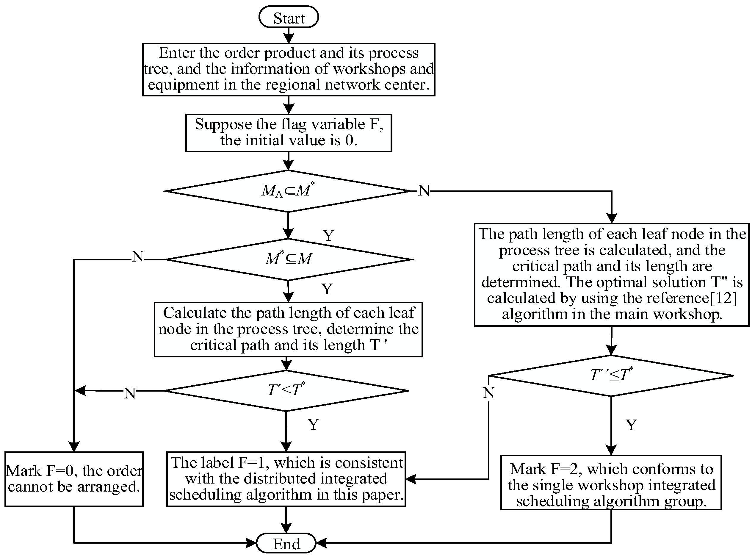
The flow chart of the distributed comprehensive scheduling decision strategy (Algorithm 1) is shown in Figure 1, and the specific steps are as follows:

Algorithm 1 Distributed integrated scheduling strategy

Step 1: Input the order and its process tree and the information of each workshop and equipment in the regional network center; Step 2: Set the flag variable F; the initial value is 0; Step 3: Judge whether the main workshop equipment is complete; if $M_A\subset M^{\ast }$, turn to Step 4; otherwise, turn to Step 7; Step 4: If $M^{\ast }\subset M$, turn to Step 5; otherwise, turn to Step 11; Step 5: Calculate the path length of each leaf node of the process tree, determine the critical path and the critical path length T′; Step 6: If $T^{\prime }\le T^{\ast }$, turn to Step 7; otherwise, turn to Step 11; Step 7: Calculate the path length of each leaf node in the process tree, determine the critical path and the critical path length T″, and use the reference [12] algorithm to calculate the optimal solution T″ in the main workshop; Step 8: If $T″\le T^{\ast }$, turn to Step 10; otherwise, turn to Step 9; Step 9: Mark F = 1, that is, the order conforms to the distributed integrated scheduling algorithm of this paper; turn to Step 12; Step 10: Mark F = 2, that is, the order conforms to the single workshop integrated scheduling algorithm; turn Step 12; Step 11: Mark F = 0, that is, the order cannot be arranged; Step 12: End, return to F.

3.2. Workpiece Sorting Strategy

Because the order has a delivery time limit, the completion time of the key parts of the order must be less than the delivery time. The static TUD of the workpiece is the difference between the earliest completion time and the delivery time of the workpiece. The larger the difference, the greater the influence of the completion time of the workpiece on the completion time of the product. The critical workpiece is the process sequence of the critical path in the current reverse process tree, and its static TUD is the largest. The overall structure of the reverse process tree is analyzed. The key factor affecting its completion time is the completion time of the current critical path. The key factor affecting the completion time of the reverse process forest that deletes the critical path is the completion time of the sub-tree with the longest critical path. Recursion, so the reverse process tree is recursively sorted from large to small according to the static TUD of the workpiece, and the scheduling order of the workpiece is determined by the sorting result. The sorted workpieces are represented by the sequence of operations it contains; that is, after sorting, N linked lists $Listi(1\le i\le N)$ with the same number of leaf nodes in the initial reverse process tree are obtained.

3.3. Distributed Integrated Scheduling Strategy

3.3.1. Analysis of Distributed Integrated Scheduling Strategy

After the order of the single-product manufacturing enterprise is analyzed by the distributed integrated scheduling decision strategy, if the mark F = 1, it indicates that the order needs the auxiliary production of the outsourcing equipment in the network. In the internet workshop, the equipment of the main workshop A is searched for the nearest and the same function. The outsourcing equipment is composed of the jth (j = 1) virtual symmetrical outsourcing workshop B, and the average transportation time ${\mathrm{t}}_{\mathrm{j}}$ of the equipment of workshop B and workshop A is used as the workpiece migration time between A and B.

On the premise of satisfying the delivery time of the order, when the quasi-scheduling scheme set of the workpiece is obtained after the trial scheduling of the corresponding legal processing time in the main workshop and the outsourcing workshop, the quasi-scheduling scheme with the minimum total cost of the current workpiece migration is selected as the workpiece scheduling scheme $P_i$ of the workpiece. If it is not unique, the scheme that minimizes the processing time of the workpiece in the outsourcing workshop is selected. When the quasi-scheduling scheme set of the ith (2 ≤ i ≤ N) workpieces cannot be established based on the workpiece scheduling scheme of the (i − 1)th job and the symmetrical second workshop equipment, the (j + 1) symmetrical virtual outsourcing workshop C is continued to be established for workshop A. The average transportation time $t_{j+1}$ of each equipment in workshop C and workshop A is used as the workpiece migration time between A and C, j = j + 1. Then, based on the workpiece scheduling scheme of the (i − 1)th workpiece and the symmetrical (j + 1) workshop equipment, all the processes contained in the ith workpiece are rescheduled, so as to establish the workpiece scheduling scheme of the ith workpiece.

3.3.2. Algorithm Design of Distributed Integrated Scheduling Strategy

(1)

Establish the basic scheduling scheme

The key workpieces are only processed in the main workshop that accepts the order, and the basic scheduling scheme only schedules the processes on the longest process sequence. The processes contained in the key workpieces are serially constrained, so the reverse scheduling method is adopted. The processing start time of the root node is “0”, and the processes contained in the first workpiece List1 are sequentially scheduled in the main workshop, and the first workpiece scheduling scheme $P_1$ is established.

(2)

Establish the ith workpiece scheduling scheme

Taking $P_{i-1}$ as the basic scheduling scheme, the process of establishing $P_i$ is more complicated. For each process, it is first judged whether it can be processed in the main workshop. Create a job scheduling algorithm for the ith workpiece (Algorithm 2). The pseudo code is as follows:

Set an array of spare outsourcing workshops: preWorkshop[]. The array elements are composed of two fields: outsourcing workshop (ws) and migration time (t). The array elements are arranged in ascending order of t.

Algorithm 2 Establishing the workpiece scheduling plan for the ith workpiece

1: Flag = false; 2: wsIdx = 0; 3: wsCount = 0; 4: t = preWorkshop[wsIdx].t; 5: For (m = 1; m ≤ K; m++)//There are K processes in Listi 6:   success = false; 7:   while (!success) 8:     Initialize the quasi-scheduling scheme set: Pm(X) = null; 9:     For (j = 1; j ≤ QT.length; j++) 10:      QSS = null; 11:      Establish a temporary debugging scheme: PTemp; 12:      If (Flag) 13:        Listi.TUD ± t; 14:      If (PTemp.totaltime ≤ T*) 15:        If (|Listi.TUD| ≥ t) 16:          PTemp is added to QSS; 17:          Update the value of Listi.TUD; 18:          Flag = false; 19:        Else 20:          The process from m + 1 to K in Listi is tested and scheduled in the main workshop in turn, and a temporary debugging scheme is established: PTempRest; 21:          Update the value of Listi.TUD; 22:          If (PTempRest.totaltime ≤ T*) 23:            PTempRest is added to QSS; 24:            Flag = false; 25:          Else 26:            If (Successfully schedule the mth process in Listi in the outsourcing shop preWorkshop[wsIdx].ws) 27:              wsCount = wsIdx + 1; 28:              Add the scheduling results to QSS; 29:              Listi.TUD ±t; 30:              Flag = true; 31:            End If 32:      End If 33:      Else 34:        If (Successfully schedule the mth process in Listi in the outsourcing shop preWorkshop[wsIdx].ws 35:          wsCount = wsIdx + 1; 36:          Add the scheduling results to QSS; 37:          Listi.TUD ± t; 38:          Flag = true; 39:        End If 40:      If (QSS != null) 41:        Add QSS to Pm(X); 42:      End If 43:    End For 44:  If (Pm(X) != null) 45:    success = true; 46:    In Pm(X), the quasi-scheduling scheme with the lowest cost of job migration is selected to join baseP. If not unique, the quasi-scheduling scheme with the least processing time of preWorkshop [wsIdx].ws is selected to join baseP. 47:  Else 48:    wsIdx++; 49:  End While 50: End For

4. Algorithm Design and Complexity Analysis

4.1. Algorithm Design

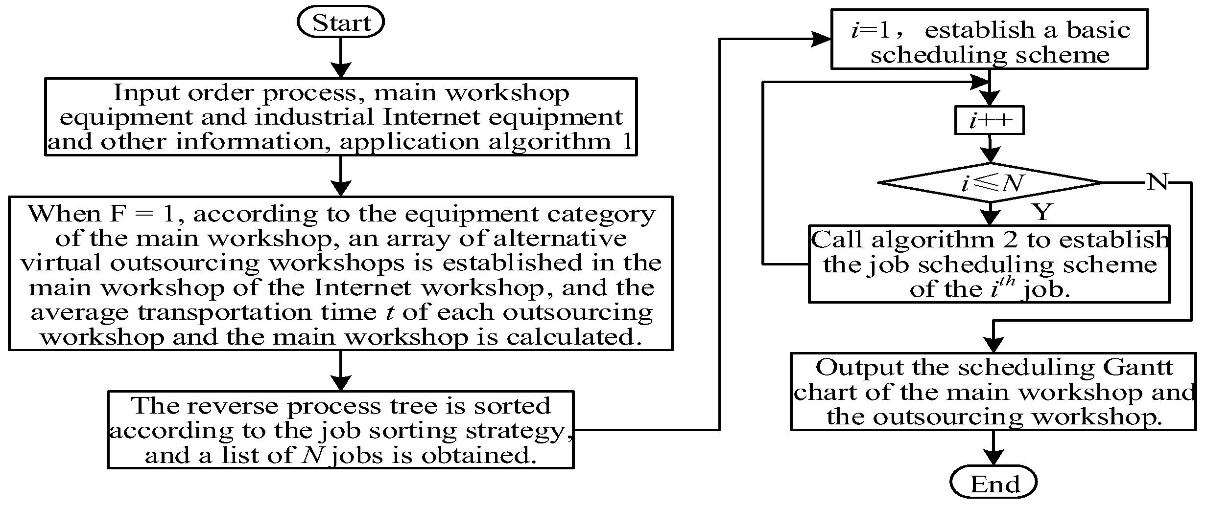
The flow chart of the integrated scheduling algorithm (Algorithm 3) considering the workpiece TUD and its migration cost is shown in Figure 2, and the specific steps are as follows.

Algorithm 3 RISA-WTUDMC algorithm

Step 1: Input order product process information, main workshop equipment information, and industrial internet equipment information; apply Algorithm 1; Step 2: When the flag F = 1, according to the main workshop equipment category, an alternative virtual outsourcing workshop array is established in the internet workshop for the main workshop, and the average transportation time t of each virtual outsourcing workshop and the main workshop is obtained. Step 3: The reverse process tree is sorted according to the workpiece sorting strategy to obtain a list Listi (1 ≤ i ≤ N) that stores the processes contained in N jobs. Step 4: i = 1, establish the basic scheduling scheme $P_1$ (the first workpiece scheduling scheme), i++. Step 5: Determine whether i ≤ N is established; if yes, turn to Step 8; if no, turn to Step 9. Step 6: Call Algorithm 2 to establish the workpiece scheduling scheme $P_i$ of the ith job. Step 7: Generate the scheduling Gantt chart of the main workshop and the outsourcing workshop and output it.

4.2. Complexity Analysis

The complexity of the algorithm in this paper is determined by the complexity of Step 2, Step 3, and Step 5 in Algorithm 3. They are independent of each other, so the complexity of the total algorithm is the maximum of the complexity of these three algorithms.

(1)

For process trees of complex products, symmetric-structure products exhibit high consistency in geometric configuration, dimensions, and processing sequences. In contrast, branch nodes of asymmetric-structure products show substantial differences due to customized design requirements and manufacturing constraints, which is due to the customized design requirements of products or on-site manufacturing constraints. Although there are differences between the two types of process architectures, each node in the tree structure corresponds to an independent processing procedure, forming a complete and continuous product manufacturing process in series. For the reverse-order process tree with n nodes, it is necessary to traverse n nodes to calculate the average transportation time between the virtual outsourcing workshop and the main workshop, and the time complexity is O(n).

(2)

The core operation of the process of sorting the process sequence is to sort the leaf nodes of the process tree. The worst case is that the process tree has n − 1 leaf nodes; assuming that the bubble method is used to sort, the time complexity is O(n²).

(3)

The complexity of step 4 is determined by the number of processes K of Listi; the greater the K, the greater the complexity, and vice versa. Obviously, K << n; in order to simplify the analysis here, let K = n. The first process of Listi is traversed at all quasi-scheduling time points of the required equipment in the main control workshop or the outsourcing workshop. In the worst case, the number of quasi-scheduling time points of the first process is far less than n. Traverse the remaining processes of Listi at all quasi-scheduling time points of the required equipment in the main control workshop or the outsourcing workshop. So, its complexity is O(n²).

In summary, the time complexity of the proposed algorithm is O(n²).

5. Examples and Comparative Analysis

5.1. Example Elaboration

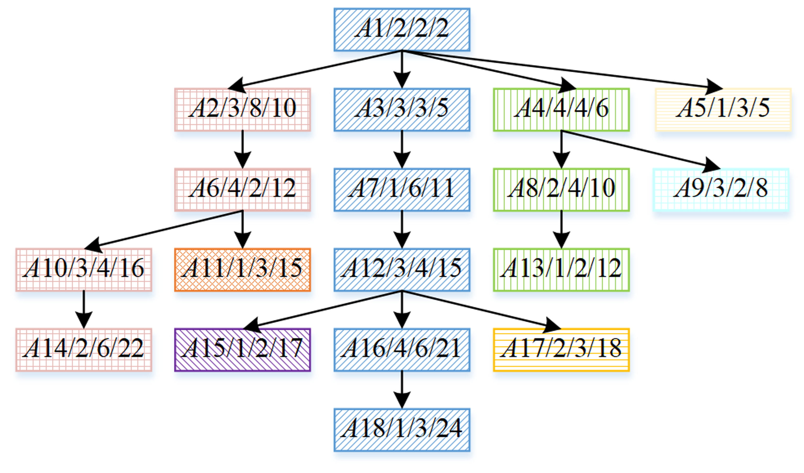
Assuming that there is a single complex product order A received by a single-product manufacturing enterprise, the number of processes of product A is 18, the required processing equipment is four types, the processing time unit is working hours, and the order due date is denoted as T* (working hours). The reverse process tree of product A is shown in Figure 3.

Assuming that the workshop equipment of the enterprise is sufficient, the workshop containing the required four types of equipment is named as the main workshop, and the average transportation time from the four types of equipment in the workshop of other internet enterprises to the main workshop is t = 2 h, and they are virtualized in the outsourcing workshop B.

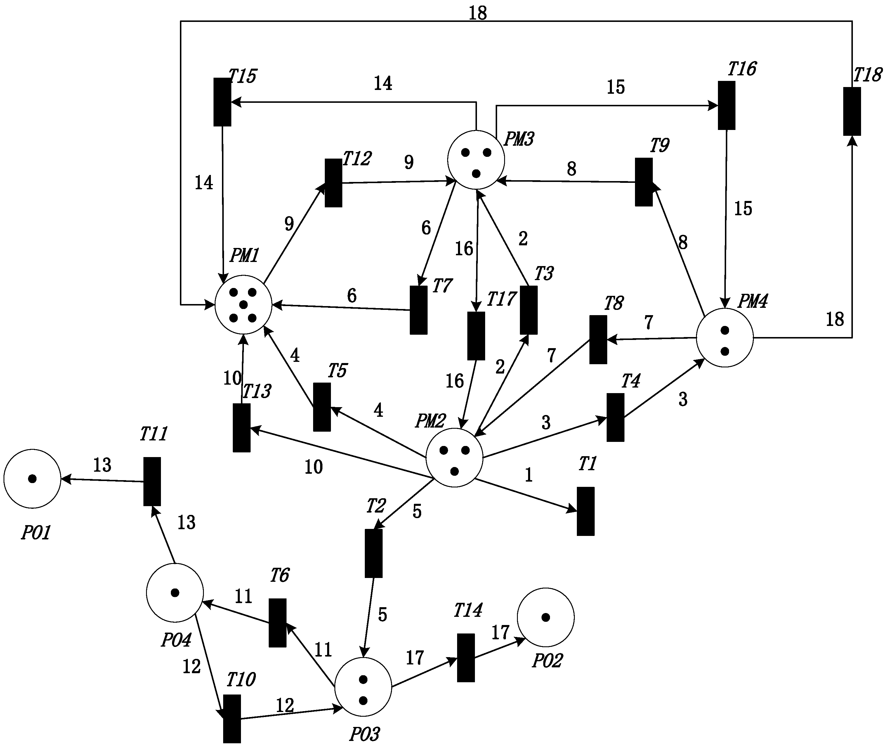
In this paper, the basic Petri net is used for modeling and simulation, and the Petri net model of the reverse process tree of complex product A is established by using Platform Independent Petri Net Editor V4.3. Through Petri net modeling, it can intuitively describe the constraints of process sequence and equipment parallelism in integrated scheduling, which is convenient for process simulation and state deduction. Here, the place is represented by a circular node; the transition is represented by a short vertical line; a directed arc is used to represent the relationship between place-directed transitions and the relationship between transitions and places. The token value is calculated by the algorithm.

In the Petri net modeling diagram shown in Figure 4, the places PM1–PM4 represent the main workshop equipment M1–M4 in the complex product A scheduling system, PO1–PO4 represent the equipment M1–M4 in the symmetrical outsourcing workshop, and the transitions T1–T18 correspond to the process A1–A18. Where PM1 corresponds to five transitions: T5, T7, T13, T15, and T18; place PM2 corresponds to three transitions: T1, T8, and T17; the PM3 corresponds to three transitions: T3, T9, and T12; place PM4 corresponds to two transitions: T4 and T16; PO1 corresponds to the transition T11; PO2 corresponds to the transition T14; PO3 corresponds to transitions T2 and T10; PO4 corresponds to transition T6. There are three states between place and transition as follows:

(1)

Concurrency state: Each disjoint transition is preferentially excited in its own place.

(2)

The sequential state with tight constraints between transitions: Only when the tight constraint transition of the transition excites and releases the token can it have the token in the corresponding place and enter the excitation state.

(3)

The order state of the place constraint relationship between transitions: Only after the current transition is triggered can the next transition in the same place have a token.

In order to verify the optimization effect of the algorithm proposed in this paper, the representative methods matching the research scenarios and problem constraints in this field are selected: the single-workshop integrated scheduling algorithm considering the time urgency of the workpiece in reference [12] (SWISA) and the two-workshop integrated scheduling algorithm based on timing in reference [15] (ISA-TWBOT). Both algorithms are studied for the integrated scheduling problem of complex tree-structured products. As the latest and typical scheduling algorithm published in this direction, this paper uses it as a comparison benchmark to verify the effectiveness and superiority of the proposed algorithm.

(1)

Using a single-workshop integrated scheduling algorithm to schedule product A

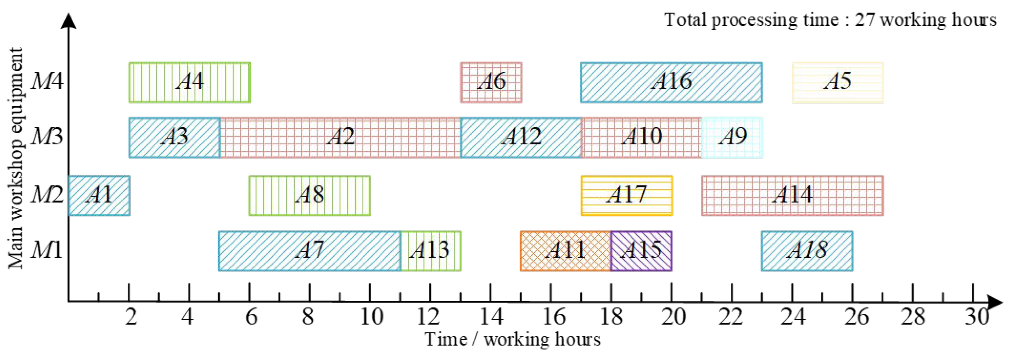
The processes included in the critical path of product A are A1, A3, A7, A12, A16, and A18, and the critical path length is 24 working hours. The integrated scheduling algorithm considering the process sequence TUD in reference [12] and reference [13] is applied to schedule product A in the main workshop, and the same product scheduling Gantt chart is obtained as shown in Figure 5. The total processing time of the product is 27 h.

(2)

Using a distributed integrated scheduling algorithm to schedule product A

When the delivery time meets 24 h ≤ T* < 27 h, the main workshop of the single-product manufacturing enterprise cannot complete the order production task alone. The main workshop and the outsourcing workshop participate in the processing together, assuming that T* = 24 h.

The reverse process tree of product A is divided into eight jobs by the job sorting strategy, and the processes contained in each workpiece are stored in the Listi (1 ≤ i ≤ 8):

The elements in List 1 of the first workpiece are A1, A3, A7, A12, A16, and A18;

The elements in List 2 of the second workpiece are A2, A6, A10, and A14;

The element in List 3 of the third workpiece is A11;

The element in List 4 of the fourth workpiece is A17;

The element in List 5 of the fifth workpiece is A15;

The elements in List 6 of the sixth workpiece are A4, A8, and A13;

The element in List 7 of the seventh workpiece is A9;

The element in List 8 of the eighth workpiece is A5.

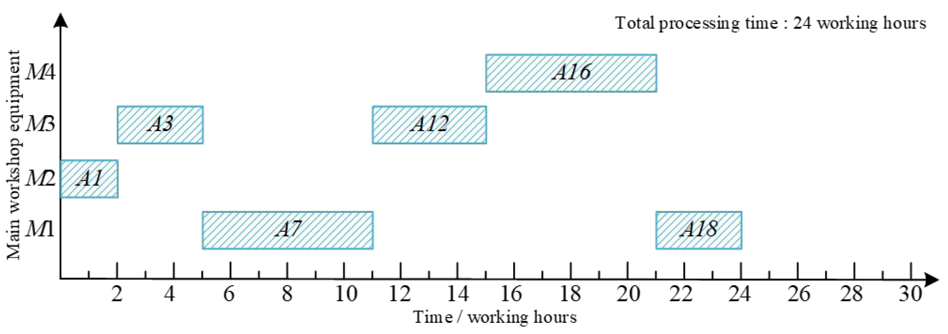
The reverse scheduling method is used to schedule the first workpiece in the main workshop to obtain its workpiece scheduling scheme. The Gantt chart is shown in Figure 6, and the total processing time is 24 h.

Based on the workpiece scheduling scheme of the first workpiece, try to schedule the second workpiece in the main workshop. The quasi-scheduling time points of process A2 are 2, 5, and 15, respectively. At the time points of 2 and 5, the insertion process A2 does not meet the delivery date requirements. At the time point of 15, although the temporary scheme after the trial scheduling process A2 meets the delivery time requirement, the TUD of the second workpiece is equal to the ideal completion time minus the delivery time, which is equal to (15 + 8 + 2 + 4 + 6) − 24 = 11 > 0, and the TUD of the workpiece needs to be less than or equal to 0, so this phenomenon will not occur. Based on the temporary scheme formed by inserting A2 into time point 15, the remaining subsequent processes A6, A10, and A14 contained in the second workpiece cannot be arranged in the main workshop during the delivery period, so time point 15 is not desirable.

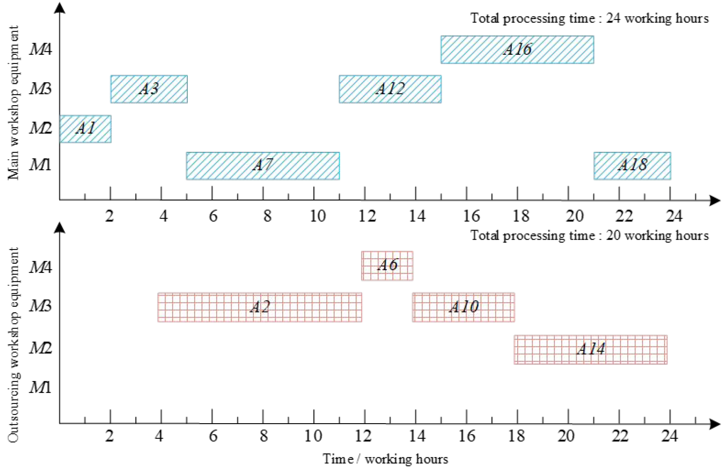
In actual production, A2 needs to be migrated back to the main workshop after the completion of the outsourcing workshop and processed together with A3, A4, and A5 into A1. The starting processing time of A2 in the outsourcing workshop is the sum of the processing end time and the migration time of A1, that is, 2 + 2 = 4. At time point 4, the process A2 is arranged on equipment M3 of the outsourcing workshop to start processing, and the processing end time point is 4 + 8 = 12. The quasi-scheduling time points are 14 and 21 to judge whether the post-process A6 of A2 can be processed in the main workshop, which is the same as the way to judge process A2. The only quasi-scheduling scheme is obtained by scheduling A10 and A14 in turn as the workpiece scheduling scheme of the second workpiece, and the Gantt chart is shown in Figure 7.

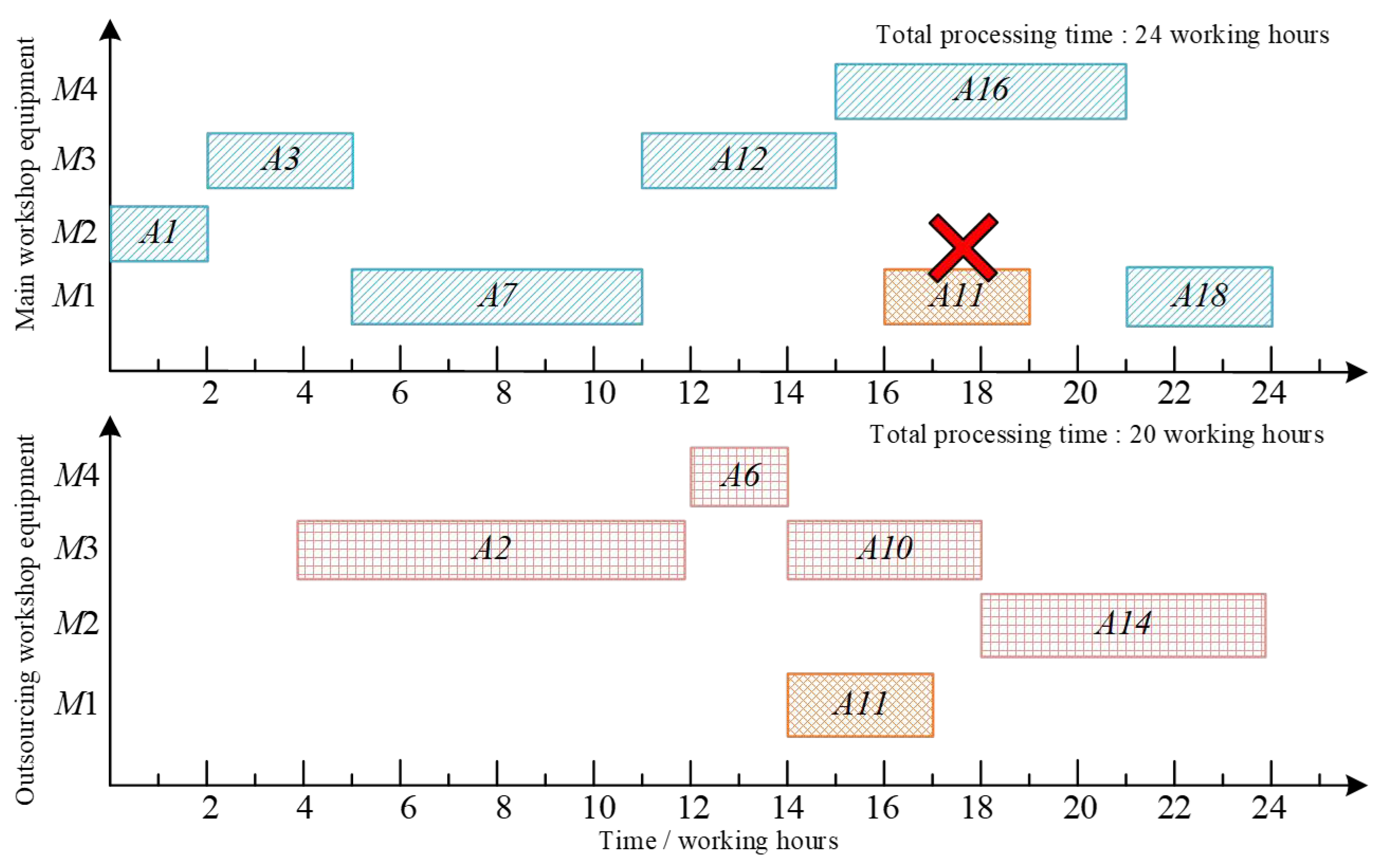
On the basis of the job scheduling scheme of the second workpiece, the first quasi-scheduling scheme of the third workpiece is established by scheduling the process A11 of the third workpiece in the main workshop, and the processing time point is 16. The process A11 of the third workpiece is scheduled in the outsourcing workshop, and the processing time point is 14. The second quasi-scheduling scheme of the third workpiece is established. In actual production, because the first quasi-scheduling scheme will cause the third workpiece to produce two migration costs, the first time from the main workshop to the outsourcing workshop, the second time is to migrate back to the main workshop with the second workpiece of the outsourcing workshop to participate in the processing A1; in the second quasi-scheduling scheme, the third workpiece only generates one migration cost from outsourcing to the main workshop. Therefore, the second quasi-scheduling scheme with the smallest total cost of the current migration is selected as the workpiece scheduling scheme for the third workpiece. The Gantt chart is shown in Figure 8.

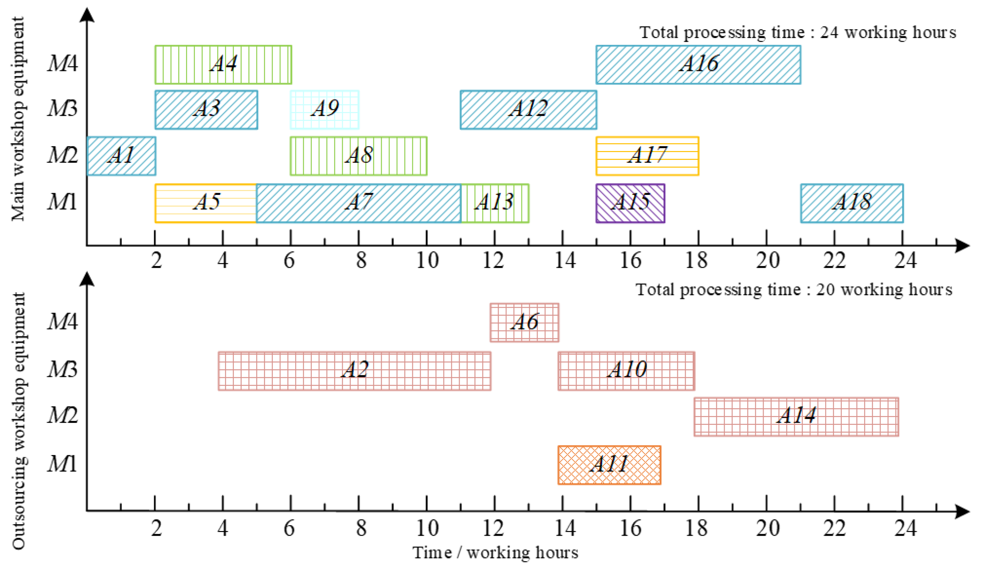
The Gantt chart of scheduling order A using the algorithm in this paper is shown in Figure 9. In the production process of integrated scheduling, the migration cost $C_T$ of the second and third workpieces from the outsourcing workshop to the main workshop is generated, that is, $C_T=K_3\times (2+2)=4K_3$, and the commission cost $C_Y$ of the total processing time of the outsourcing equipment is generated, that is, $C_Y=K_2\times 23=23K_2$. In this case, the total processing time of the main workshop is 24 h, and the total processing time of the outsourcing workshop is 20 h.

For order A with a critical path length of 24 man-hours, the production cycle of order A can be shortened to its static critical path length by using the auxiliary processing of a symmetrical virtual outsourcing workshop with an average transportation time of not more than 2 man-hours in the industrial internet workshop and the enterprise’s main workshop, and the goal of 24 man-hours delivery can be achieved. At the same time, in the process of integrated scheduling, the migration cost of the workpiece is minimized, and the outsourcing commission is minimized, so as to maximize the benefits of the single-product manufacturing enterprise. In summary, the effectiveness of the proposed algorithm is fully illustrated.

5.2. Comparative Analysis

In order to illustrate the effectiveness of the proposed algorithm, the proposed algorithm is compared with the typical two-workshop integrated scheduling reference [15], ISATWBOT, in the same research field.

In reference [15], the migration time between symmetrical workshops is 5 h, the critical path length of product A is 22 h, and the total processing time of product A is also 22 h. Therefore, the order delivery time is set to 22 h.

The reverse process tree of the product shown in Figure 12 in reference [15] is divided into seven workpieces by using the workpiece sorting strategy in this paper. The operations contained in each workpiece are stored in the Listi:

The first workpiece contains processes: A1, A3, A8, A14, A19, A22, A23, and A24.

The second workpiece contains processes: A2, A7, A13, A18, and A21.

The third workpiece contains processes: A12 and A17.

The fourth workpiece contains processes: A5, A10, A16, and A20.

The fifth workpiece contains the process: A11.

The sixth workpiece contains processes: A4, A9, and A15.

The seventh workpiece contains the process: A6.

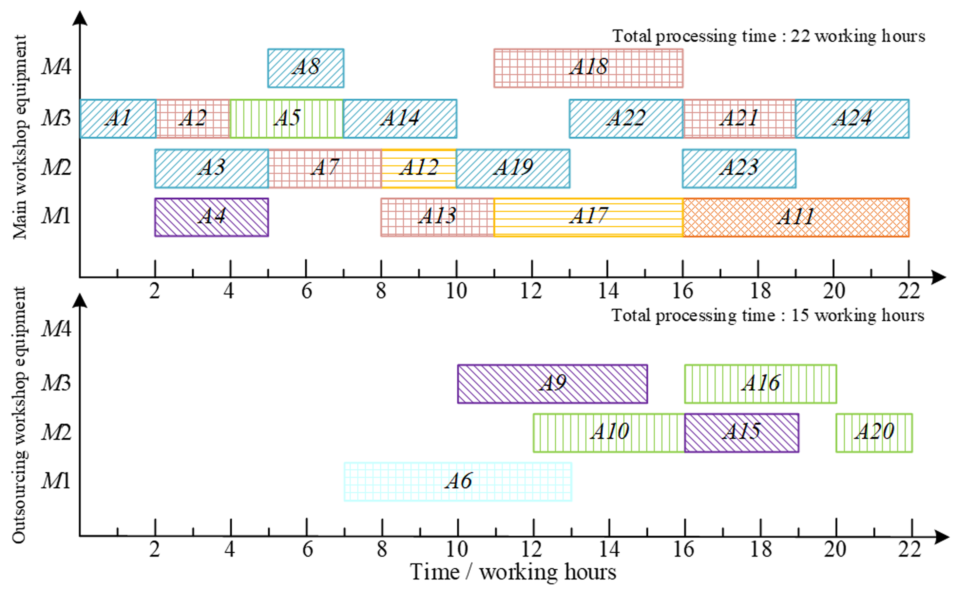
Using the reverse scheduling method, the workpiece scheduling scheme $P_1$ is obtained by scheduling the first workpiece in the main workshop. Based on the $P_1$ scheme, a workpiece is used as the unit for trial scheduling each time. In the main workshop and the outsourcing workshop, the processes contained in the remaining jobs are trial-scheduled in turn to obtain the set of workpiece quasi-scheduling schemes for the workpiece. On the basis of satisfying the delivery time of 22 h, the workpiece quasi-scheduling scheme with the smallest job migration cost is selected as the workpiece scheduling scheme. If not unique, the scheme that minimizes the machine processing time of the outsourcing workshop is selected. The job scheduling scheme $P_7$ of the 7th workpiece is the order scheduling scheme P. The Gantt chart of the product scheduling results in the algorithm scheduling reference [15] is shown in Figure 10. The comparison table of scheduling results is shown in

Table 1. Schedule result comparison table (working hours).

Algorithm	Analysis Index
	${\mathit{T}}_{\mathit{P}\mathit{Z}}\left({\mathit{S}}_1\right)$	${\mathit{T}}_{\mathit{P}\mathit{W}}\left({\mathit{S}}_2\right)$	Total Processing Time (S1)	Total Processing Time (S2)	Total Time of Workpiece Migration (Working Hours)
RISA-WTUDMC	57	24	22	15	15
ISA-TWBOT	51	30	22	19	20

.

From Figure 10, it can be seen that in the process of applying the algorithm in this paper to schedule product A, the migration cost $C_T$ of the 4th, 6th, and 7th workpieces from the outsourcing workshop to the main workshop is generated, that is, ${\mathrm{C}}_{\mathrm{T}}={\mathrm{K}}_3\times (5+5+5)=15K_3$, and the commission cost $C_Y$ of 24 h of processing in the outsourcing workshop is generated, that is, $C_Y=\times 24=24K_2$. In the integrated scheduling process of reference [15], the migration cost ${\mathrm{C}}_{\mathrm{T}}$ of the 4th, 5th, 6th, and 7th workpieces from the outsourcing workshop to the main workshop is generated, that is, $C_T=K_3\times (5+5+5+5)=20K_3$, and the commission cost $C_Y$ of 30 working hours in the outsourcing workshop is generated, that is, $C_Y=K_2\times T_{PW}=K_2\ast 30=30K_2$, $(15K_3+24K_2)<(20K_3+30K_2)$.

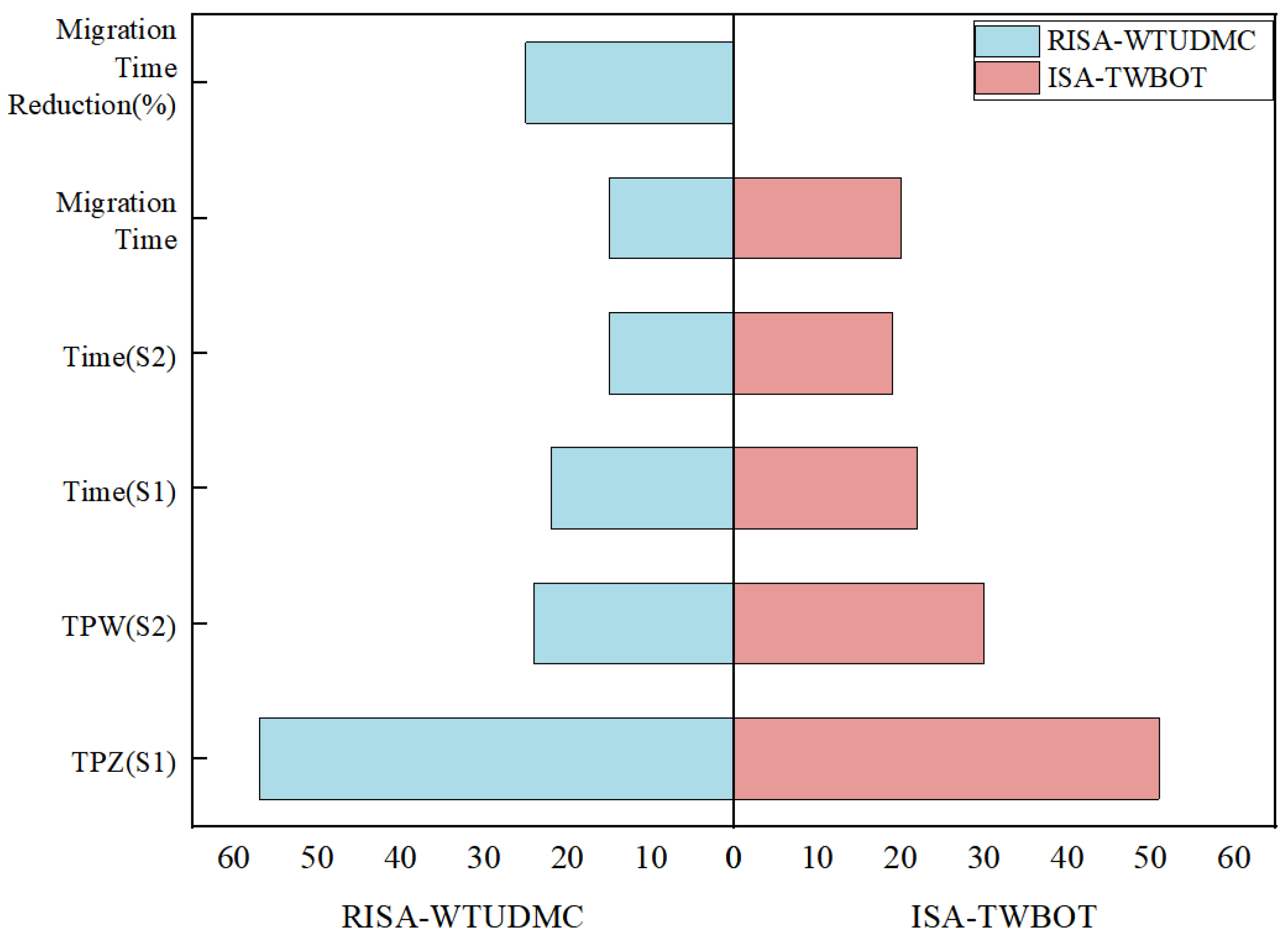
As shown in Figure 11, it can be clearly seen that the total time of workpiece migration in this algorithm is less, which realizes the processing of as many processes as possible in the main workshop, thus reducing the migration cost of process processing. Therefore, compared with the algorithm proposed in reference [15], the migration cost of the algorithm proposed in this paper is lower, the total time of process migration is reduced by 25%, and the total time of outsourcing processing is shortened by 20%, indicating that the algorithm in this paper has better performance in solving practical problems.

5.3. Comparative Analysis of Data Sets

The algorithm proposed in this paper has a wide range of versatility and universality. It can be scheduled for any other symmetric or asymmetric complex products with tree structure. In order to fully verify the adaptability and superiority of the algorithm to different-scale product processing scenarios, the experiment set up multiple sets of test examples with a process scale as low as 20 and a maximum of 500. The process trees used in all comparative experiments in this paper are randomly generated by computers. The generation rules of random process trees follow the general generation logic of tree product instances in the field of integrated scheduling: the generated process trees strictly meet the topological characteristics of tree products, and each process has a legal tight-front–tight-back constraint relationship to ensure that the process processing logic has no closed-loop conflict. The root node represents the total task of the product, and the remaining child nodes correspond to each processing procedure. The process randomly allocates the precursor process to ensure that the generated instance can generate both a symmetrical tree structure and an asymmetric tree structure, which can cover a variety of complex product process features.

This experiment was completed on a local computer. The experimental hardware environment is as follows: the CPU is an Intel i7 processor (LENOVO, Beijing, China); memory 16 GB; software environment: Windows operating system; MATLAB R2021b experimental environment; 150 examples of complex product process tree with tree structure were randomly selected and divided into [20, 40, 80, 100, 200, and 500] six kinds of data. On average, 25 process trees were selected for each group of data; that is, 20, 40, 80, 100, 200, and 500 processes were included in each process tree for experiments, and the processing end time of each group of data was compared. The experimental process is a deterministic scheduling construction algorithm. There is no iterative optimization process and no iterative stopping criterion. The termination condition of the algorithm is that the current process tree completes the scheduling allocation, all processes obtain the legal start time and completion time, and the scheduling process ends naturally. The scheduling decision in this section takes the completion time as the priority target, and the outsourcing cost coefficient and the migration cost coefficient take fixed values for the cost index record, which do not affect the process workshop allocation and completion time results. Therefore, the maximum number of virtual outsourcing workshops is set to five, the maximum number of equipment is 10, the migration time is 2 working hours, the outsourcing cost coefficient is 1.5, and the migration cost coefficient is 2.

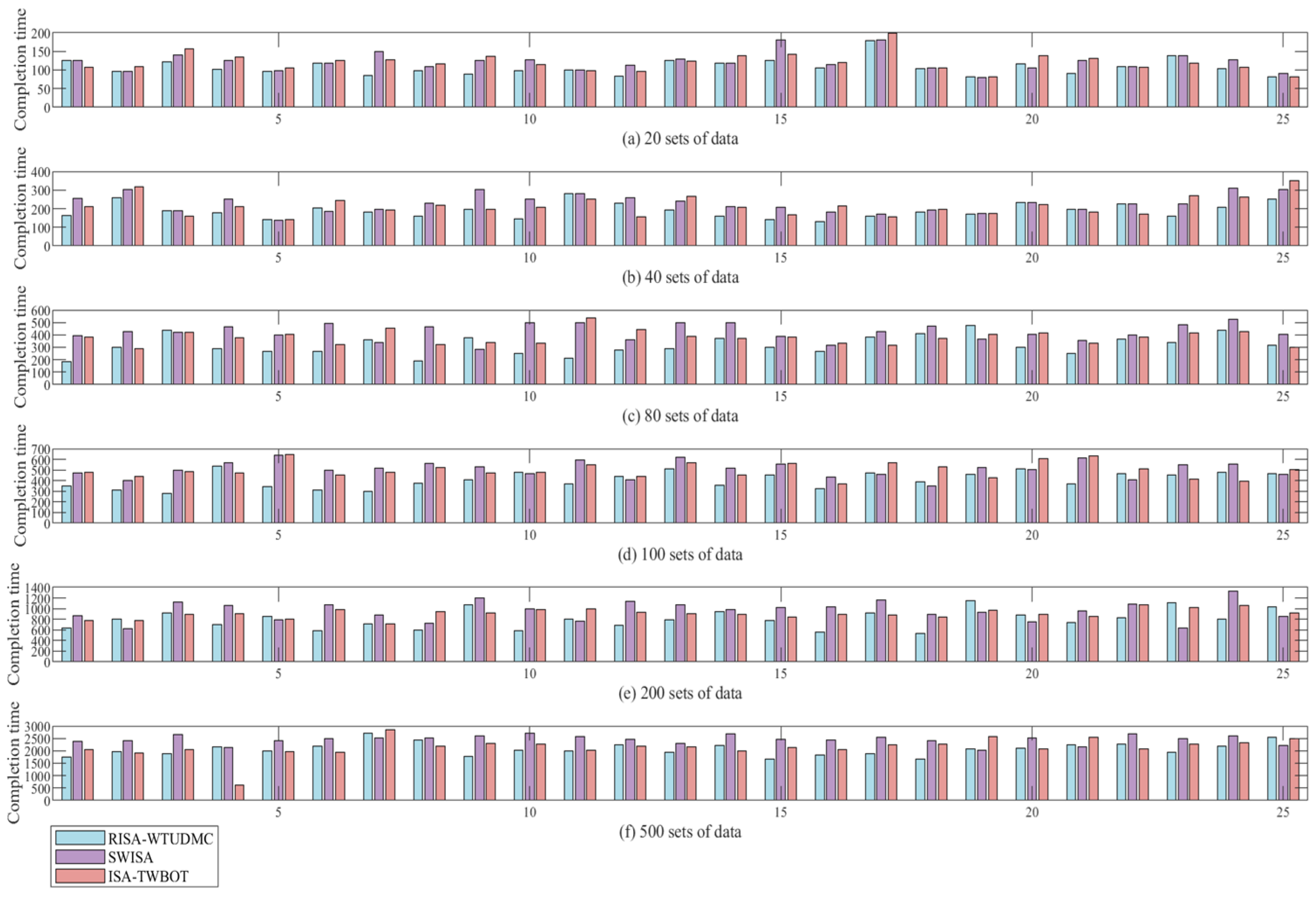
The scheduling results of the algorithm proposed in this paper (RISA-WTUDMC), the application of the single-shop integrated scheduling algorithm (SWISA), and the algorithm proposed in reference [15] (ISA-TWBOT) are shown in Figure 12. The experimental results show that with the increasing number of processes, in most cases, the total processing time of the proposed algorithm is earlier than that of the other two comparison algorithms, and it can maintain a relatively stable total processing time without performance degradation. Therefore, the scheduling effect of the proposed algorithm on each operation scale is better, which further shows that the proposed algorithm can better adapt to the scheduling requirements of small- and medium-sized and large-scale complex products, and provide a feasible reference for actual production scheduling.

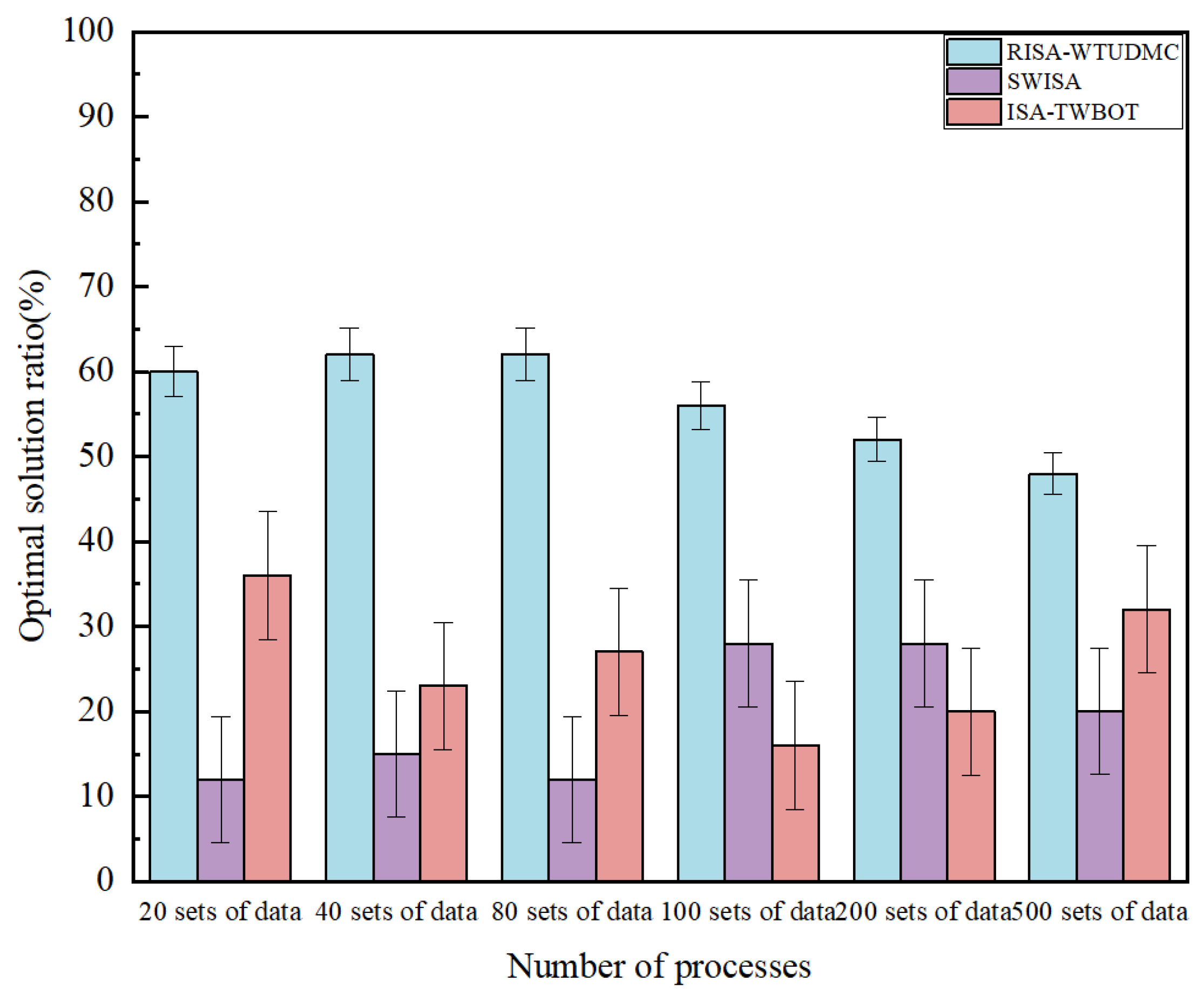
In order to further quantify the quality of different algorithms, the optimal solution ratio index is introduced to carry out comparative experiments. The experimental results are shown in Figure 13. For the same test process tree instance, the minimum completion time obtained by the three comparison algorithms is regarded as the reference optimal completion time of the example. The proportion of the optimal solution of an algorithm represents the percentage of the sample whose output is equal to the reference optimal completion time in the total sample of the group. Each group contains 25 independent random examples. The column height in the figure is the value of the optimal solution ratio of each group. The error bar in the figure represents the standard deviation of the corresponding index, which is used to reflect the degree of discrete fluctuation in the internal results of 25 groups of samples. The higher the optimal solution ratio, the closer the solution obtained by the algorithm is to the optimal solution, and the better the performance of the algorithm. It can be seen from the mean and standard deviation in the figure that under the large-scale complex examples of small-scale and 500 processes, the algorithm in this paper not only has a significantly higher mean value of the optimal solution ratio than the comparison algorithm, but also maintains the standard deviation of the sample in a reasonable range, indicating that the algorithm has a small fluctuation in the solution result, has good stability, and can stably obtain a better completion time.

Based on the above experimental results of random tree complex product process trees with different process scales, from the analysis of the two core performance indicators of total processing time and optimal solution ratio, it can be concluded that under the same test conditions, for the complex product integrated scheduling problem studied in this paper, these two comparison algorithms are not as good as the algorithm in this paper in terms of the rationality of process scheduling, the control of migration cost, and the reduction in total processing time. The algorithm in this paper establishes a symmetrical outsourcing workshop to coordinate the process scheduling and reasonably allocates the process processing tasks. Combined with the proportion of the optimal solution and its confidence interval results, it can be seen that whether it is a small-scale simple process tree or a highly complex multi-process product, the algorithm in this paper shows higher practicability and superiority in practical applications, which can stably achieve lower total processing time and better meet the production scheduling requirements of distributed complex products.

5.4. Sensitivity Analysis

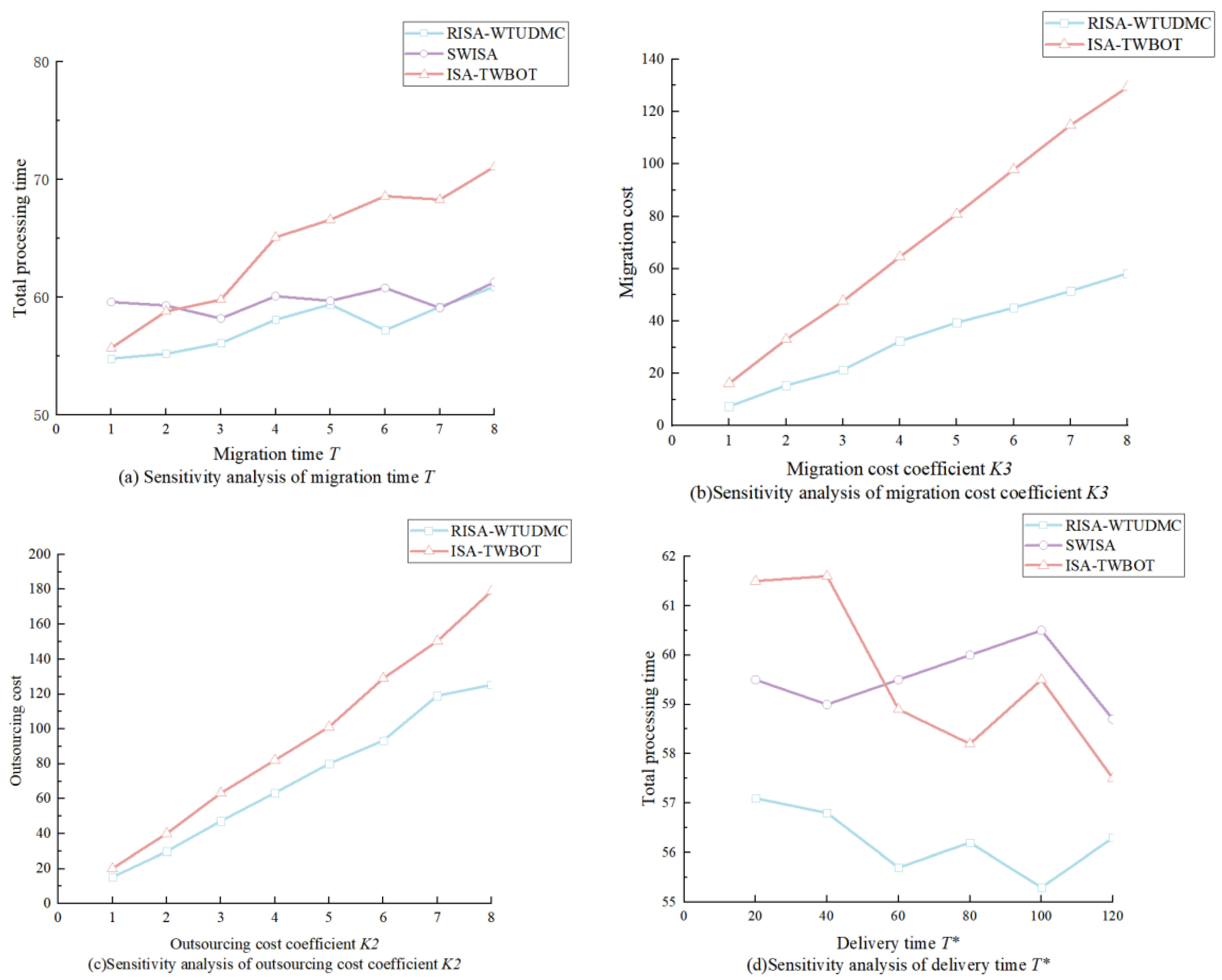
In order to verify the stability of the algorithm in different production environments, a medium-scale example of randomly generating a complex product process tree with 40 processing operations is selected. The sensitivity experiments are carried out for the migration time T, the migration cost coefficient K3, the outsourcing cost coefficient K2, and the delivery time T*. All experimental groups are run 50 times to obtain the mean value and are compared with the SWISA algorithm and the ISA-TWBOT algorithm (because SWISA is a single-shop integrated scheduling algorithm, there is no outsourcing workshop, so the sensitivity analysis of this algorithm is not included in Figure 14b,c), as shown in Figure 14. It can be seen from the figure that the algorithm in this paper is more stable under various parameter fluctuations. The ISA-TWBOT algorithm is more sensitive to changes in various parameters, while SWISA is limited to the single workshop scenario without outsourcing, which further proves that the algorithm in this paper is more robust and stable in the complex scheduling environment.

The above single-parameter experiment only controls the change in a single variable, and the remaining parameters remain unchanged, reflecting the influence of independent disturbance of a single factor on the scheduling results. However, in the actual distributed manufacturing production scenario, the migration time of the workpiece, the migration cost coefficient, and the outsourcing cost coefficient often fluctuate synchronously. The three types of parameters have obvious interactive coupling effects, and the univariate experiment cannot reflect the real robustness of the algorithm under multi-factor linkage.

To this end, this paper selects the migration time T, the outsourcing cost coefficient K2, and the migration cost coefficient K3, three parameters that have a core impact on the distributed collaborative scheduling results, to carry out multi-parameter coupling experiments. Combined with the value range of the scheduling scene parameters in this paper and the parameter interval of the previous single-parameter sensitivity experiment, the low-level value of 1, the benchmark level value of 4, and the high-level value of 8 are set for the three parameters. Among them, the low level represents the ideal production conditions of centralized workshop location, low outsourcing service quotation, and small workpiece transfer loss; the benchmark level corresponds to the conventional actual working conditions of most enterprises under the industrial internet collaborative manufacturing; the high level represents the extreme conditions of cross-regional outsourcing, high transportation costs, and time-consuming workpiece migration. The three-level setting not only covers the complete parameter interval under ideal, normal, and extreme conditions in actual production, but also captures the influence of linear and nonlinear changes in parameters on scheduling performance.

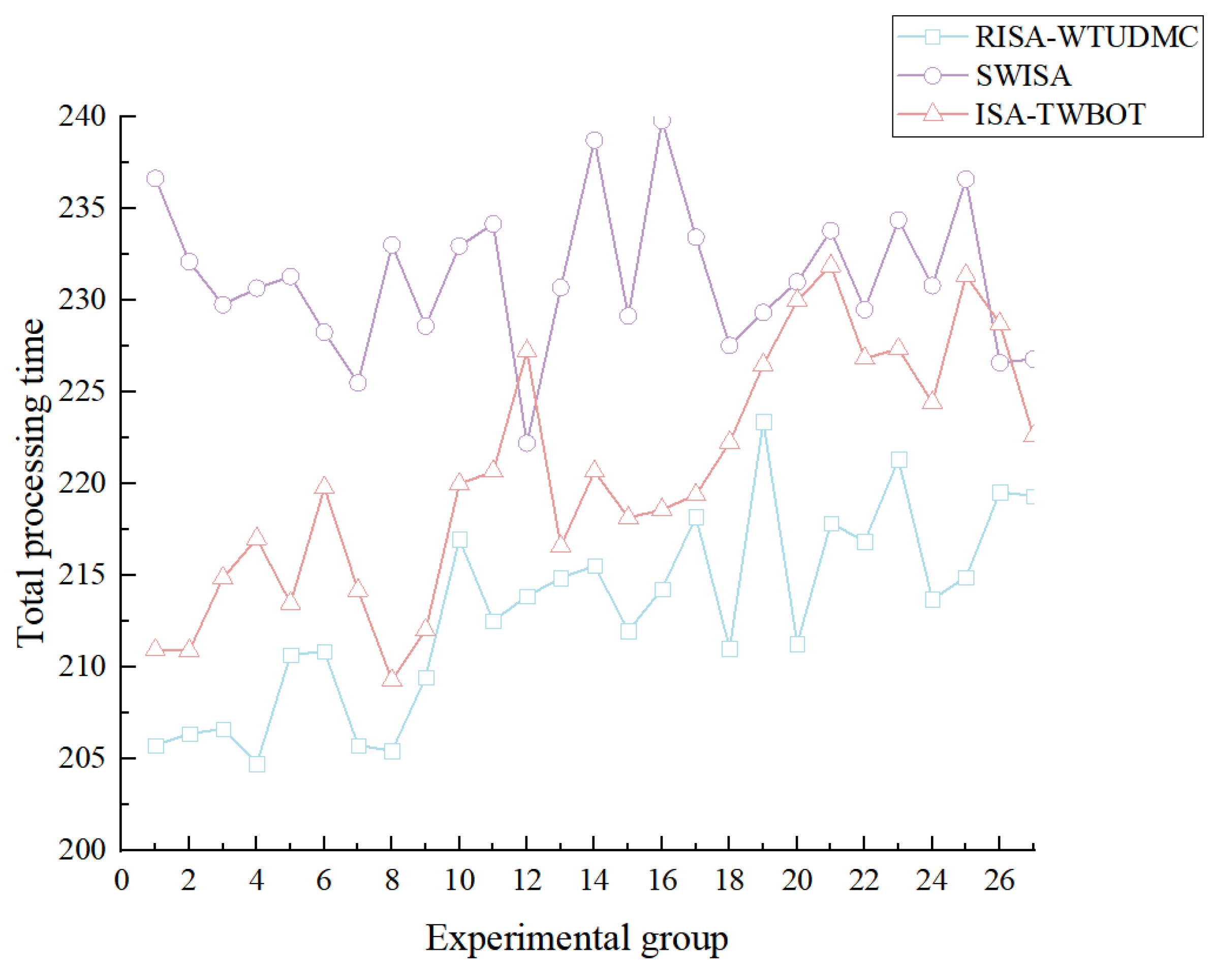
The 3 × 3 × 3 full factorial experimental design was used to traverse all 27 sets of parameter combinations. Compared with a small number of orthogonal experiments, the full factorial experiment can completely analyze the main effects of the three parameters, the interaction effects of the two parameters, and the higher-order interaction effects of the three parameters. The potential coupling effect between the parameters will not be missed, and the deviation of the experimental results and the one-sided conclusion caused by a small amount of orthogonal working condition sampling will be avoided from the root, so as to objectively test the stability of the algorithm under the large-scale fluctuation of the parameters. Each group of working conditions runs independently and repeatedly 50 times, and the average total processing time is taken as the evaluation index. The experimental results are shown in Figure 15.

It can be seen from Figure 15 that under 27 sets of multi-parameter synchronous disturbance conditions, the average total processing time obtained by the RISA-WTUDMC algorithm proposed in this paper is lower than that of SWISA and ISA-TWBOT in all test combinations. At the same time, the data fluctuation of the output results of the algorithm is smaller, showing stable solution performance. Although the migration time, the outsourcing cost coefficient, and the migration cost coefficient change together, the algorithm in this paper can still maintain a better scheduling effect. The full factor coupling experiment fully proves that, in the face of the complex working conditions of synchronous fluctuation of multiple production constraints in a distributed manufacturing environment, the algorithm in this paper has better solution stability, which can effectively alleviate the risk of schedule delay caused by multi-factor linkage disturbance, and is more suitable for the changing production site under internet collaborative manufacturing.

5.5. Applicability and Potential Limitations Analysis

The reverse integrated scheduling algorithm considering the time urgency degree and migration cost of the workpiece proposed in this paper is suitable for the distributed collaborative scheduling scenario of tree-shaped complex products with tight-front and tight-back constraints. For the multi-workshop collaborative production mode, when the enterprise needs to take into account the delivery time constraint, the outsourcing workshop processing cost, and the workpiece migration cost, the algorithm can complete the process allocation and the outsourcing workshop processing process selection decision according to the actual situation, and optimize the product completion time, which has reference value for multi-variety and small-batch equipment manufacturing and production. In industries such as multi-variety and small-batch mechanical equipment manufacturing, the algorithm in this paper can adapt to diversified production tasks, optimize the production mode of small-batch and multi-variety, and improve the flexibility of production.

In addition, the algorithm in this paper also has potential limitations. Based on the static scheduling model, this study simplifies the actual production scene. As the scale of product processes grows, computational overhead increases, especially for heavy-industry applications characterized by complex equipment operating conditions and numerous influencing factors. In the face of very large-scale scheduling examples, the real-time performance of the solution will be restricted, which may affect the accuracy and practicability of the algorithm. In this regard, the intelligent optimization algorithm can be introduced in combination with the scheduling strategy in this paper to cope with sudden working conditions, reduce the computational complexity under the premise of ensuring production efficiency, and improve the solving ability under large-scale working conditions.

In summary, the proposed algorithm has good applicability in the static distributed collaborative integrated scheduling scenario, which can effectively improve production efficiency and reduce costs. However, its applicability and effectiveness may vary according to different industries and production scales. Therefore, this algorithm can be customized according to its own actual situation when it is used to ensure that the algorithm can maximize its effectiveness.

6. Summary

Against the background of single-product manufacturing enterprises equipped with in-house workshops and supported by industrial-internet-connected external workshops, this paper addresses the integrated-scheduling problem for orders with due-date constraints and develops a reverse integrated scheduling algorithm considering workpieces’ time-urgency degree and migration cost. Through the comparative analysis with typical algorithms, the following conclusions can be drawn:

(1)

The workpiece scheduling strategy based on workpiece TUD proposed in this paper gives priority to the operations contained in the static workpieces with large TUD and optimizes the integrated scheduling results.

(2)

The distributed integrated scheduling strategy proposed in this paper reduces the total cost of workpiece migration on the basis of meeting the order delivery time. In the case of equal total cost of workpiece migration, the processes contained in as many workpieces as possible are processed in the main workshop, thereby improving the profit of the single-product manufacturing enterprise.

(3)

The algorithm in this paper is an innovative integrated scheduling problem proposed for a single workshop of internet companies. It breaks the constraints of limited equipment resources in previous studies on integrated scheduling problems, meets the development needs of the “Internet+” manufacturing industry, and provides a practical solution for single-product manufacturing companies.

References

1. Luo, P.W.; Zhao, X.R.; Zhang, L.L.; Luo, C. An Effective Hybrid Local Search Method for Flexible Job-Shop Scheduling Problem in Smart Manufacturing Systems. Electronics 2026, 15, 2465. [Google Scholar] [CrossRef] [Scilit]
2. Wang, M.J.; Cai, J.N.; Hu, D.; Hu, Y.Q.; Han, Z.; Li, S. AI-based robots in industrialized building manufacturing. Front. Eng. Manag. 2025, 12, 59–85. [Google Scholar] [CrossRef] [Scilit]
3. Huo, B.F.; Miao, L. Distributed hybrid Flow Shop batch scheduling based on HGNN-MADRL. Comput. Integr. Manuf. Syst. 2025, 31, 4633–4662. [Google Scholar] [CrossRef]
4. Tao, M.X.; Li, X.P.; Zhou, Y.P. Distributed hybrid Flow Shop scheduling optimization based on improved Mayfly algorithm. Mach. Tool Hydraul. 2026, 54, 149–157. [Google Scholar] [CrossRef]
5. Tan, Q.M.; Ye, C.M.; Tan, X.; Zhang, M.T.; Kong, L.Y. Distributed flexible Job Shop scheduling with Dynamic Transport Time Based on Workpiece characteristics. Manuf. Autom. 2026, 48, 119–128. [Google Scholar] [CrossRef]
6. Lai, C.L.; Liu, J.J.; Liu, T.; Qiu, J.H. Look-ahead-enabled real-time scheduling in dynamic distributed assembly job shops with batch parts transfer. Comput. Ind. Eng. 2026, 219, 112167. [Google Scholar] [CrossRef] [Scilit]
7. Xie, Z.Q. Study on Operation Scheduling of Complex Product with Constraint Among Jobs. Ph.D. Thesis, Harbin University of Science and Technology, Harbin, China, 2009. [Google Scholar]
8. Li, S.Y.; Han, K.; Pei, Z.; Yi, W.C.; Lv, R.F. Green flexible job shop integrated scheduling optimization for machines and AGVs based on the INSGA-II algorithm. Proc. Inst. Mech. Eng. Part B J. Eng. Manuf. 2026, 240, 477–494. [Google Scholar] [CrossRef] [Scilit]
9. Zhang, J.X.; Deng, Q.W.; Luo, Q.; Deng, K.D.; Liao, M.Q.; Lei, Y. Integrated scheduling of green production with flexible preventive maintenance and customer-side workers by a learning-based coevolutionary algorithm. Robot. Comput.-Integr. Manuf. 2026, 98, 103140. [Google Scholar] [CrossRef] [Scilit]
10. Ge, Z.P.; Wang, H.F. Integrated Optimization of Blocking Flowshop Scheduling and Preventive Maintenance Using a Q-Learning-Based Aquila Optimizer. Symmetry 2023, 15, 1600. [Google Scholar] [CrossRef] [Scilit]
11. Fu, Y.P.; Wang, F.Q.; Li, Z.Y.; Tian, G.D.; Pham, D.T.; Sun, H. Multiobjective integrated scheduling of disassembly and reprocessing operations considering product structures and stochastic processing time via reinforcement learning-based evolutionary algorithms. Complex Intell. Syst. 2025, 11, 292. [Google Scholar] [CrossRef] [Scilit]
12. Cao, W.C.; Xie, Z.Q.; Yang, J.; Zhan, X.J.; Pei, L.R.; Yu, X. A Reverse Order Hierarchical Integrated Scheduling Algorithm Considering Dynamic Time Urgency Degree of the Process Sequences. Electronics 2022, 11, 1868. [Google Scholar] [CrossRef] [Scilit]
13. Cao, W.C.; Xie, Z.Q.; Pei, L.R. Reverse Order and Greedy Integrated Scheduling Algorithm Considering Dynamic Time Urgency Degree of the Process Sequences. J. Electron. Inf. Technol. 2022, 44, 1572–1580. [Google Scholar] [CrossRef]
14. Wu, H.Z.; Wu, Z.Y.; Wang, Y.; Mark, G. Integrated scheduling of pallets and vehicles for automated warehouses with multi-tier racks. Eng. Appl. Artif. Intell. 2026, 163, 112851. [Google Scholar] [CrossRef] [Scilit]
15. Zhang, X.H.; Xie, Z.Q.; Xin, Y.; Yang, J. Integrated Scheduling Algorithm of Two Workshops Based on Optimal Time. Comput. Integr. Manuf. Syst. 2017, 23, 1938–1949. [Google Scholar] [CrossRef]
Figure 1. Flow chart of decision strategy for distributed integrated scheduling.
Symmetry 18 01444 g001
Figure 2. Flow chart of integrated scheduling algorithm considering workpiece TUD and its migration cost.
Symmetry 18 01444 g002
Figure 3. Reverse process tree of product A.
Symmetry 18 01444 g003
Figure 4. Petri net modeling of product A.
Symmetry 18 01444 g004
Figure 5. Application of the single-workshop integrated scheduling algorithm to schedule the Gantt chart of product A.
Symmetry 18 01444 g005
Figure 6. Gantt chart of the workpiece scheduling scheme for the first workpiece.
Symmetry 18 01444 g006
Figure 7. The Gantt chart of the workpiece scheduling scheme for the second workpiece.
Symmetry 18 01444 g007
Figure 8. Gantt chart of the workpiece scheduling scheme for the third workpiece.
Symmetry 18 01444 g008
Figure 9. Apply the algorithm proposed in this paper to schedule the Gantt chart of product A.
Symmetry 18 01444 g009
Figure 10. The Gantt chart of the product in the proposed algorithm scheduling ISA-TWBOT is applied.
Symmetry 18 01444 g010
Figure 11. Comparative analysis of the processing indexes of the algorithm and ISA-TWBOT algorithm.
Symmetry 18 01444 g011
Figure 12. Comparative analysis of three algorithms scheduling 150 random instances.
Symmetry 18 01444 g012
Figure 13. The optimal solution ratio of three algorithms.
Symmetry 18 01444 g013
Figure 14. Sensitivity analysis of four types of parameters.
Symmetry 18 01444 g014
Figure 15. Multi-parameter coupling sensitivity analysis.
Symmetry 18 01444 g015