Adaptive Prescribed-Time Tracking Control for Output-Constrained Hydraulic Servo Systems with Time-Varying Parameters

Abstract

This paper proposes an adaptive prescribed-time tracking control strategy based on the dynamic surface technique for hydraulic servo systems subject to time-varying parameters, external disturbances, and output constraints. First, a state-constrained transformation function is introduced to convert the strict output constraint condition into an error boundedness problem. Meanwhile, the dynamic surface control (DSC) technique is employed to effectively avoid the “explosion of complexity” inherent in traditional backstepping design. Second, to tackle complex uncertainties, prescribed-time-driven adaptive update and disturbance estimation laws are separately formulated for precise parameter learning and active disturbance feedforward compensation. Furthermore, a smooth nonlinear robust term is specifically integrated to suppress the residual errors induced by parameter adaptation. Based on the transformed system, a novel control framework integrating error constraints, adaptive parameter estimation, and prescribed-time performance is developed. Rigorous Lyapunov stability analysis proves that the proposed controller not only strictly prevents the system output from violating the constraint boundaries throughout the entire operation, but also ensures that the tracking error converges rapidly and smoothly to a small bounded region near the origin within a time that can be independently predetermined by the designer. Finally, the effectiveness and superiority of the proposed control strategy are fully validated through simulations.

1. Introduction

Advanced nonlinear control strategies have been extensively investigated to enhance the transient and steady-state performance of complex mechanical systems [1,2,3]. As a typical high-end equipment, electro-hydraulic proportional servo systems have been widely applied in aerospace mechanisms and intelligent robots due to their high power-to-weight ratio and rapid response capabilities. However, achieving high-performance motion control remains a significant challenge because these systems exhibit severe nonlinearities and uncertainties. Consequently, rapidly and effectively eliminating the effects of various uncertainties to achieve precise tracking performance has become a primary focus for researchers [4,5].

In the field of nonlinear tracking control, finite-time control has gradually emerged as a mainstream strategy due to its guaranteed settling time and excellent tracking accuracy [6,7,8,9]. However, the actual convergence time of finite-time controllers is highly dependent on the initial conditions of the system. To overcome this limitation, fixed-time control strategies were developed [10,11,12] in which the upper bound of the settling time is independent of the initial states. Nevertheless, the estimated upper bound in fixed-time control is often overly conservative and heavily depends on the controller design parameters. To overcome the limitations of both finite-time and fixed-time methods, the prescribed-time control framework has been widely adopted [13]. This framework ensures that the convergence time of the tracking error can be preassigned arbitrarily by the user, completely independent of the system’s initial conditions and design parameters [14,15].

Despite the excellent transient performance provided by prescribed-time control, the aforementioned controllers often neglect the state and output constraints that inherently exist in practical systems. In practical engineering, systems are strictly required to operate under specific constraints due to physical limitations and safety requirements [16]. Ignoring these constraints can severely compromise system stability and operational safety. To address this, the barrier Lyapunov function (BLF) provides an effective mechanism to prevent constraint violations [17,18]. However, in the traditional control framework combining the BLF method with backstepping, the repeated differential computation of virtual controllers leads to the well-known “explosion of complexity” issue as the system order increases. To address this dilemma, the Dynamic Surface Control (DSC) technique and command filtered backstepping have been introduced [19,20]. By employing a first-order filter, the DSC scheme elegantly avoids the analytical differentiation of virtual control signals, thereby significantly simplifying the controller design process.

While the integration of DSC and prescribed-time control effectively handles constraints and computational burdens, another critical issue remains unresolved. In the existing literature [6,7,8,9,10,11,12,20], the uncertain parameters of the nonlinear system are conventionally assumed to be unknown constants. In practical hydraulic systems, however, considering component wear and temperature variations, unknown parameters (such as friction coefficients and internal leakage) are inherently time-varying. The simplification of treating time-varying parameters as constants severely degrades the system’s dynamic control performance. To tackle this, some researchers have explored advanced adaptive architectures and robust compensation schemes to separately handle parameter uncertainties and time-varying disturbances [21,22]. However, these advanced frameworks typically rely on asymptotic stabilization or complex switching mechanisms, lacking the capability to guarantee error convergence within a preassigned time. Moreover, traditional adaptive controllers designed for slowly time-varying systems often fail to cope with high-frequency time-varying fluctuations, leading to high-gain chattering and threatening actuator reliability [23,24].

To bridge the aforementioned gaps, this paper proposes an adaptive prescribed-time tracking control strategy based on the dynamic surface technique for output-constrained hydraulic servo systems subject to time-varying parameters and external disturbances. The main contributions of this paper are summarized as follows:

• Output-Constrained Prescribed-Time DSC Framework: A novel state-dependent constraint transformation combined with the dynamic surface control (DSC) technique is proposed. Unlike traditional barrier Lyapunov function (BLF) methods that impose strict feasibility conditions and suffer from the “explosion of complexity” in backstepping designs [17,18], the introduced transformation function seamlessly maps the constrained physical output into an error boundedness problem without violating the original state boundaries. Furthermore, by embedding a prescribed-time function directly into the DSC framework, the proposed controller ensures that the system output strictly respects physical safety limits while eliminating tedious analytical differentiations, laying a solid foundation for high-precision rapid tracking.
• Synergized Prescribed-Time Parameter Adaptation and Active Disturbance Compensation: Distinct from conventional adaptive schemes limited by constant-parameter assumptions [6,7,8,9,10,11,12,20], a novel prescribed-time learning architecture is developed to separately handle complex time-varying uncertainties. By ingeniously embedding the prescribed-time performance function into the update laws, parameter adaptation and disturbance estimation mechanisms are independently formulated to achieve precise parameter learning and active disturbance feedforward compensation. Furthermore, to avoid severe parameter coupling and high-gain chattering caused by conventional over-adaptation, a smooth nonlinear robust term is specifically integrated to suppress the residual errors left uncompensated by parameter adaptation. This synergized mechanism guarantees that the tracking errors converge strictly within the user-defined time frame.

This article proceeds as follows: Section 2 introduces the dynamic modeling and problem formulation. Section 3 elaborates on the dynamic surface-based adaptive prescribed-time control scheme, complemented by a rigorous stability proof. Following this, Section 4 offers simulation results to corroborate the theoretical claims. Finally, Section 5 concludes the paper, summarizing the main findings and outlining future work prospects.

2. Problem Statement and Preliminaries

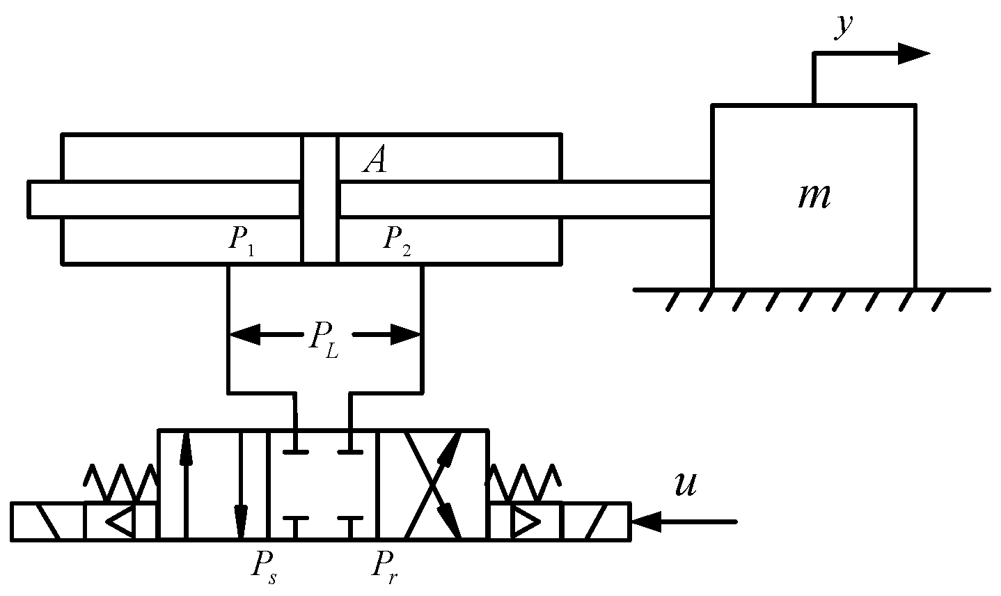
The simplified model of the hydraulic servo system under study is illustrated in Figure 1. Under normal operating conditions, the load is driven by the piston rod of a hydraulic cylinder, which is controlled by a valve.

According to Figure 1 and Newton’s second law, the force balance equation of the hydraulic system is given by

$$m\ddot{y}=A{P}_1-A{P}_2-B\dot{y}+D_1(t)$$

(1)

where $m$ denotes the load mass; $y$, $\dot{y}$, and $\ddot{y}$ represent the displacement, velocity, and acceleration of the hydraulic cylinder piston rod, respectively; $A$ is the effective acting area of the piston; $P_1$ and $P_2$ denote the oil pressures in the supply and return chambers of the cylinder, respectively; $B$ is the viscous damping coefficient; $D_1(t)$ represents the unmodeled mechanical disturbance; and $t$ denotes time.

Neglecting the external leakage of the hydraulic cylinder, the pressure dynamic equations can be expressed as

$$\begin{array}{l}{\dot{P}}_1={\beta }_e(-A\dot{y}-C_t{P}_L+Q_1+q_1)/V_1\\ {\dot{P}}_2={\beta }_e(A\dot{y}+C_t{P}_L-Q_2-q_2)/V_2\end{array}$$

(2)

where ${\beta }_e$ denotes the effective bulk modulus of the hydraulic oil; $C_t$ is the internal leakage coefficient of the cylinder; $P_L=P_1-P_2$ represents the load pressure difference; $V_1=V_{01}+Ay$ and $V_2=V_{02}-Ay$ are the control volumes of the supply and return chambers, respectively, with $V_{01}$ and $V_{02}$ being the corresponding initial volumes; $Q_1$ and $Q_2$ denote the flow rates of the supply and return chambers, respectively; $q_1$ and $q_2$ represent the unmodeled disturbances in the pressure dynamics; and ${\dot{P}}_1$ and ${\dot{P}}_2$ denote the time derivatives of $P_1$ and $P_2$.

Assuming that the control input $u$ is proportional to the spool displacement $x_v$ of the electro-hydraulic proportional servo valve, the flow rates $Q_1$ and $Q_2$ can be expressed in terms of $x_v$ as follows

$$\begin{array}{l}{Q}_1=k_q{x}_v\left(s(x_v)\sqrt{P_s-P_1}+s(-x_v)\sqrt{P_1-P_r}\right)\\ Q_2=k_q{x}_v\left(s(x_v)\sqrt{P_2-P_r}+s(-x_v)\sqrt{P_s-P_2}\right)\end{array}$$

(3)

where $k_q=C_d{w}_0\sqrt{2/\rho }$ is the flow gain coefficient of the valve, with $C_d$, $w_0$, and $\rho$ being the discharge coefficient, the area gradient of the valve spool, and the density of the hydraulic oil, respectively; $P_s$ and $P_r$ denote the supply pressure and the return pressure, respectively; and $s(\chi )$ represents a function of the intermediate variable, defined as

$$s(\chi )=\left\{\begin{array}{l}1\hspace{1em}if\hspace{1em}\chi \ge 0\\ 0\hspace{1em}if\hspace{1em}\chi <0\end{array}\right.$$

(4)

where $\chi$ is the scalar argument.

Furthermore, given the relationship $x_v=k_{i}u$, where $k_i$ denotes the voltage-to-spool displacement gain coefficient, Formula (3) can be rewritten as

$$\begin{array}{l}{Q}_1=k_u{R}_{1}u\\ Q_2=k_u{R}_{2}u\end{array}$$

(5)

where the intermediate variables are defined as $k_u=k_q{k}_i$, $R_1=s(u)\sqrt{P_s-P_1}+s(-u)\sqrt{P_1-P_r}$, and $R_2=s(u)\sqrt{P_2-P_r}+s(-u)\sqrt{P_s-P_2}$.

Define the state vector as $\iota ={[{\iota }_1,{\iota }_2,{\iota }_3]}^T={[y,\dot{y},(A{P}_1-A{P}_2)/m]}^T$, where the state variables are chosen as ${\iota }_1=y$, ${\iota }_2=\dot{y}$, and ${\iota }_3=(A{P}_1-A{P}_2)/m$. Consequently, Formula (1) can be transformed into the following state-space equation

$$\begin{array}{l}{\dot{\iota }}_1={\iota }_2\\ {\dot{\iota }}_2={\iota }_3-{\vartheta }_2{\psi }_2+d_2\\ {\dot{\iota }}_3=g_{1}u-f_1-{\vartheta }_3{\psi }_3+d_3\end{array}$$

(6)

where ${\dot{\iota }}_1$, ${\dot{\iota }}_2$, and ${\dot{\iota }}_3$ denote the first-order time derivatives of ${\iota }_1$, ${\iota }_2$, and ${\iota }_3$.

In which

$$\left\{\begin{array}{l}{d}_2=D_1(t)/m,d_3={\beta }_{e}A{q}_1/m{V}_1+{\beta }_{e}A{q}_2/m{V}_2\hfill \\ g_1=(A{R}_1/m{V}_1+A{R}_2/m{V}_2){\beta }_e{k}_u\hfill \\ {\vartheta }_2=B/m,{\psi }_2={\iota }_2\hfill \\ {\vartheta }_3=(1/V_1+1/V_2){\beta }_e{C}_t,{\psi }_3={\iota }_3\hfill \\ f_1=(A^2/m{V}_1+A^2/m{V}_2){\beta }_e{\iota }_2\hfill \end{array}\right.$$

(7)

The primary control objectives of the proposed strategy are formulated as follows:

(1) The system tracking error is rigorously driven into a tiny, bounded residual set around the origin within a user-assigned time limit.

(2) Throughout the entire operating process, the physical output signal ${\iota }_1$ strictly adheres to the predefined asymmetric safety boundaries, which can be expressed as:

$${\iota }_1\in R:-N_1<{\iota }_1<N_2$$

(8)

where $N_1$ and $N_2$ are positive constants.

(3) All signals of the closed-loop system are bounded.

In order to achieve the control objectives, the following assumption is made:

Assumption 1.

From a practical engineering perspective, the planned motion profile ${\iota }_d$ is assumed to be physically realizable, which implies that  ${\iota }_d$  and its successive derivatives up to the second order remain finite at any given time.

Assumption 2.

Due to the finite energy nature of the physical operating environment, both the time-varying parameters and the unmodeled external disturbances injected into the system are assumed to be strictly bounded. Specifically, there exist unknown positive constants  $b_i$ and $c_i$ such that $|{\vartheta }_i(t)|\le b_i$ and $|d_i(t)|\le c_i$ for $i=2,3$.

Remark 1.

Although Assumptions 1 and 2 act as fundamental theoretical premises for the nonlinear control of hydraulic servo mechanisms, their engineering implementations inherently present specific physical limitations. For Assumption 1, the differentiability condition imposed on the reference trajectory is strictly necessary to comply with the mechanical actuating limits of hydraulic components, precluding instantaneous responses to abrupt step commands. Regarding Assumption 2, environmental and unmodeled perturbations are naturally restricted by the mechanical capacities and finite energy of the hardware, guaranteeing the validity of the upper thresholds  $b_i$ and  $c_i$  ($i=2,3$). However, extreme anomalies, such as severe hardware malfunctions, could breach these presumed boundaries, inevitably threatening the global stability of the closed-loop architecture.

Remark 2.

The predefined constraint margins must be meticulously calibrated according to the actual physical attributes of the hydraulic plant, ensuring that the constrained system output is strictly confined to the safe operational envelope throughout the execution of the designed control protocol.

3. Controller Construct

3.1. Nonlinear Transformation Function

The output-state nonlinear transformation function is shown below:

$$L_1({\iota }_1)={\displaystyle \frac{{\iota }_1}{(N_1+{\iota }_1)(N_2-{\iota }_1)}}$$

(9)

According to the constructed nonlinear transformation function, it is obvious that while the initial value ${\iota }_1(0)$ satisfies $-N_1<{\iota }_1(0)<N_2$, $L_1({\iota }_1)$ tends to infinity as ${\iota }_1(t)\to -N_1$ or ${\iota }_1(t)\to N_2$.

Thus, for any initial state ${\iota }_1(0)$ that satisfies $-N_1<{\iota }_1(0)<N_2$, if the controller design ensures that $L_1({\iota }_1)$ is bounded, then $-N_1<{\iota }_1<N_2$ will naturally hold. Derivation of the nonlinear transformation function (9) yields

$${\dot{L}}_1={\mu }_1{\dot{\iota }}_1$$

(10)

$${\mu }_1={\displaystyle \frac{(N_1{N}_2+{\iota }_1^2)}{{(N_1+{\iota }_1)}^2{(N_2-{\iota }_1)}^2}}$$

(11)

where ${\dot{L}}_1$ and ${\dot{\iota }}_1$ are the first derivatives of $L_1$ and ${\iota }_1$.

The equivalent unconstrained nonlinear system is represented as follows:

$$\left\{\begin{array}{l}{\dot{\iota }}_1={\mu }_1{\iota }_2\hfill \\ {\dot{\iota }}_2={\iota }_3-{\vartheta }_2{\psi }_2+d_2\hfill \\ {\dot{\iota }}_3=g_1\mu -f_1-{\vartheta }_3{\psi }_3+d_3\hfill \end{array}\right.$$

(12)

3.2. Prescribed-Time Function

A time-varying scaling function is introduced and defined as follows:

$$\begin{array}{l}h=\left\{\begin{array}{l}{\displaystyle \frac{\eta t_h}{{(t_h-t)}^m+{\mathrm{b}}_f^n}},t\in \left[0,t_h\right)\hfill \\ {\displaystyle \frac{\eta t_h}{{\mathrm{b}}_f^n}},t\in \left[t_h,\infty \right)\hfill \end{array}\right.\\ \dot{h}=\left\{\begin{array}{l}m{(t_h-t)}^{m-1}{h}^2/(t_h\eta ),\in \left[0,t_h\right)\hfill \\ 0,t\in \left[t_h,\infty \right)\hfill \end{array}\right.\end{array}$$

(13)

in which $t_h$ represents the prescribed time. $\eta >0$, $m\ge 2$, and $n\ge 1$ represent the designable parameters and $b_f>0$ is a small positive design constant close to zero.

3.3. Controller Design

Define the following error:

$$v_1=L_1-{\alpha }_d,v_j={\iota }_j-{\alpha }_{jf},j=2,3$$

(14)

where $L_1$ denotes the nonlinear transformation function given in (9), and ${\alpha }_d$ is defined as

$${\alpha }_d={\displaystyle \frac{{\iota }_d}{(N_1+{\iota }_d)(N_2-{\iota }_d)}}$$

(15)

where ${\iota }_d$ denotes the reference signal, and ${\alpha }_{jf}$ represent the outputs of the improved command filters described below.

$${\dot{\alpha }}_{jf}=-w_{j}h{\epsilon }_j$$

(16)

where ${\epsilon }_j={\alpha }_{jf}-{\alpha }_{j-1}$ represent the filtering errors and $w_j$ are the designable parameters.

According to (14), it can be obtained that

$${\iota }_j=v_j+{\epsilon }_j+{\alpha }_{j-1}$$

(17)

Define the error-transformation functions $s_i(i=1,2,3)$ using the introduced time-varying scaling function.

$$s_i=h{v}_i$$

(18)

Step 1: Differentiating the error variable, utilizing (14) and (17) yields:

$$\begin{array}{ll}{\dot{v}}_1& ={\dot{L}}_1-{\dot{\alpha }}_d\\ & ={\mu }_1{\iota }_2-{\dot{\alpha }}_d\\ & ={\mu }_1(v_2+{\epsilon }_2+{\alpha }_1)-{\dot{\alpha }}_d\end{array}$$

(19)

where ${\dot{\alpha }}_d$ is the first derivative of ${\alpha }_d$.

Differentiating $s_1$ obtains

$$\begin{array}{ll}{\dot{s}}_1& =\dot{h}{v}_1+h{\dot{v}}_1\\ & =\dot{h}{v}_1+h({\mu }_1(v_2+{\alpha }_1+{\epsilon }_2)-{\dot{\alpha }}_d)\end{array}$$

(20)

Construct a brand new Lyapunov function $V_1$:

$$V_1={\displaystyle \frac{1}{2}}{s}_1^2$$

(21)

The derivative of $V_1$ is expressed as

$$\begin{array}{ll}{\dot{V}}_1& =s_1{\dot{s}}_1\\ & =h\dot{h}{v}_1^2+h^2{v}_1({\mu }_1(v_2+{\alpha }_1+{\epsilon }_2)-{\dot{\alpha }}_d)\end{array}$$

(22)

According to Formula (22), the virtual control law ${\alpha }_1$ can be designed as

$${\alpha }_1={\displaystyle \frac{1}{{\mu }_1}}(-k_1{s}_1+{\dot{\alpha }}_d-\dot{h}{v}_1/h-{\mu }_1^2{v}_1/h)$$

(23)

where $k_1>0$ is the designable parameter.

Substituting Formula (23) into Formula (22) gives:

$${\dot{V}}_1=-k_{1}h{s}_1^2+{\mu }_1{s}_1{s}_2+{\mu }_1{s}_1{\Xi }_2-{\mu }_1^2{v}_1{s}_1$$

(24)

where ${\Xi }_2=h{\epsilon }_2$.

Step 2: Differentiating $v_2$ obtains

$${\dot{v}}_2={\dot{\iota }}_2-{\dot{\alpha }}_{2f}={\iota }_3-{\vartheta }_2{\psi }_2+d_2-{\dot{\alpha }}_{2f}=(v_3+{\epsilon }_3+{\alpha }_2)-{\vartheta }_2{\psi }_2+d_2-{\dot{\alpha }}_{2f}$$

(25)

Differentiating $s_2$ obtains

$$\begin{array}{ll}{\dot{s}}_2& =\dot{h}{v}_2+h{\dot{v}}_2\\ & =\dot{h}{v}_2+h((v_3+{\alpha }_2+{\epsilon }_3)-{\vartheta }_2{\psi }_2+d_2-{\dot{\alpha }}_{2f})\end{array}$$

(26)

The estimation of ${\vartheta }_2$ is updated

$${\dot{\widehat{\vartheta }}}_2=-{\gamma }_{21}{h}^2{\psi }_2{v}_2-{\delta }_{21}h{\widehat{\vartheta }}_2$$

(27)

where ${\gamma }_{21}>0$ and ${\delta }_{21}>0$ are the designable parameters.

The estimation of $d_2$ is updated

$${\dot{\widehat{d}}}_2={\gamma }_{22}{h}^2{v}_2-{\delta }_{22}h{\widehat{d}}_2$$

(28)

where ${\gamma }_{22}>0$ and ${\delta }_{22}>0$ are the designable parameters.

Construct a brand new Lyapunov function $V_2$

$$V_2={\displaystyle \frac{1}{2}}{s}_2^2+{\displaystyle \frac{1}{2}}{\gamma }_{21}^{-1}{\tilde{\vartheta }}_2^2+{\displaystyle \frac{1}{2}}{\gamma }_{22}^{-1}{\tilde{d}}_2^2+{\displaystyle \frac{1}{2}}{\Xi }_2^2$$

(29)

where ${\tilde{\vartheta }}_2={\overline{\vartheta }}_2-{\widehat{\vartheta }}_2$ and ${\tilde{d}}_2={\overline{d}}_2-{\widehat{d}}_2$. ${\overline{\vartheta }}_2$ and ${\overline{d}}_2$ are the unknown constants.

The derivative of $V_2$ is expressed as

$$\begin{array}{ll}{\dot{V}}_2& =s_2{\dot{s}}_2-{\gamma }_{21}^{-1}{\tilde{\vartheta }}_2{\dot{\widehat{\vartheta }}}_2-{\gamma }_{22}^{-1}{\tilde{d}}_2{\dot{\widehat{d}}}_2+{\Xi }_2{\dot{\Xi }}_2\\ & =h\dot{h}{v}_2^2+h^2{v}_2((v_3+{\alpha }_2+{\epsilon }_3)-{\widehat{\vartheta }}_2{\psi }_2-({\overline{\vartheta }}_2-{\widehat{\vartheta }}_2){\psi }_2+{\widehat{d}}_2+({\overline{d}}_2-{\widehat{d}}_2)-{\dot{\alpha }}_{2f})\\ & -h^2{v}_2{\epsilon }_{{\vartheta }_2}{\psi }_2+h^2{v}_2{\epsilon }_{d_2}-{\gamma }_{21}^{-1}{\tilde{\vartheta }}_2{\dot{\widehat{\vartheta }}}_2-{\gamma }_{22}^{-1}{\tilde{d}}_2{\dot{\widehat{d}}}_2+h\dot{h}{\epsilon }_2^2+h^2{\epsilon }_2({\dot{\alpha }}_{2f}-{\dot{\alpha }}_1)\end{array}$$

(30)

where ${\dot{\Xi }}_2$ is the first derivative of ${\Xi }_2$; ${\epsilon }_{d_2}=d_2-{\overline{d}}_2$ and ${\epsilon }_{{\vartheta }_2}={\vartheta }_2-{\overline{\vartheta }}_2$.

According to Formula (30), the virtual control law ${\alpha }_2$ can be designed as

$$\left\{\begin{array}{l}{\alpha }_2=-k_2{s}_2+{\dot{\alpha }}_{2f}+{\widehat{\vartheta }}_2{\psi }_2-{\widehat{d}}_2-(\dot{h}+1)v_2/h-h{v}_2-{\mu }_1{v}_1+{\alpha }_{2s}\hfill \\ {\alpha }_{2s}={\displaystyle \frac{-s_2{(b_2‖{\psi }_2‖)}^2}{s_2{b}_2‖{\psi }_2‖\tanh (s_2/{\sigma }_2)+{\sigma }_2}}\hfill \end{array}\right.$$

(31)

where $k_2>0$ is the designable parameter. ${\sigma }_2<{\overline{\sigma }}_2\ll +\infty$, where ${\overline{\sigma }}_2$ is a positive constant.

Thus, substituting Formulas (27), (28) and (31) into Formula (30) gives:

$$\begin{array}{ll}{\dot{V}}_2& =-k_{2}h{s}_2^2+s_2{s}_3+s_2{\Xi }_3+h{s}_2{\epsilon }_{d_2}+h{s}_2({\alpha }_{2s}-{\epsilon }_{{\vartheta }_2}{\psi }_2)\\ & +{\gamma }_{21}^{-1}{\delta }_{21}h{\tilde{\vartheta }}_2{\widehat{\vartheta }}_2+{\gamma }_{22}^{-1}{\delta }_{22}h{\tilde{d}}_2{\widehat{d}}_2-{\mu }_1{s}_1{s}_2-h{v}_2^2-h^3{v}_2^2+h\dot{h}{\epsilon }_2^2-h{w}_2{\Xi }_2^2-h{\Xi }_2{\dot{\alpha }}_1\end{array}$$

(32)

where ${\Xi }_3=h{\epsilon }_3$.

Note that:

$$s_2({\alpha }_{2s}-{\epsilon }_{{\vartheta }_2}{\psi }_2)\le \left|s_2\right|b_2\parallel {\psi }_2\parallel -{\displaystyle \frac{s_2^2{b}_2^2{\parallel {\psi }_2\parallel }^2}{s_2{b}_2\parallel {\psi }_2\parallel \tanh (s_2/{\sigma }_2)+{\sigma }_2}}\le {\sigma }_2$$

(33)

Substituting Formula (33) into Formula (32) gives:

$$\begin{array}{ll}{\dot{V}}_2& =-k_{2}h{s}_2^2+s_2{s}_3+s_2{\Xi }_3+h{s}_2{\epsilon }_{d_2}+h{\sigma }_2\\ & +{\gamma }_{21}^{-1}{\delta }_{21}h{\tilde{\vartheta }}_2{\widehat{\vartheta }}_2+{\gamma }_{22}^{-1}{\delta }_{22}h{\tilde{d}}_2{\widehat{d}}_2-{\mu }_1{s}_1{s}_2-h{v}_2^2-h^3{v}_2^2+h\dot{h}{\epsilon }_2^2-h{w}_2{\Xi }_2^2+h{\Xi }_2{H}_2\end{array}$$

(34)

where $H_2=-{\dot{\alpha }}_1$.

Step 3: Differentiating $v_3$ obtains

$${\dot{v}}_3={\dot{\iota }}_3-{\dot{\alpha }}_{3f}=g_{1}u-f_1-{\vartheta }_3{\psi }_3+d_3-{\dot{\alpha }}_{3f}$$

(35)

Differentiating $s_3$ obtains

$${\dot{s}}_3=\dot{h}{v}_3+h{\dot{v}}_3=\dot{h}{v}_3+h(g_{1}u-f_1-{\vartheta }_3{\phi }_3+d_3-{\dot{\alpha }}_{3f})$$

(36)

The estimation of ${\vartheta }_3$ is updated

$${\dot{\widehat{\vartheta }}}_3=-{\gamma }_{31}{h}^2{\psi }_3{v}_3-{\delta }_{31}h{\widehat{\vartheta }}_3$$

(37)

where ${\gamma }_{31}>0$ and ${\delta }_{31}>0$ are the designable parameters.

The estimation of $d_3$ is updated

$${\dot{\widehat{d}}}_3={\gamma }_{32}{h}^2{v}_3-{\delta }_{32}h{\widehat{d}}_3$$

(38)

where ${\gamma }_{32}>0$ and ${\delta }_{32}>0$ are the designable parameters.

Construct a brand new Lyapunov function $V_3$:

$$V_3={\displaystyle \frac{1}{2}}{s}_3^2+{\displaystyle \frac{1}{2}}{\gamma }_{31}{\tilde{\vartheta }}_3^2+{\displaystyle \frac{1}{2}}{\gamma }_{32}{\tilde{d}}_3^2+{\displaystyle \frac{1}{2}}{\Xi }_3^2$$

(39)

where ${\tilde{\vartheta }}_3={\overline{\vartheta }}_3-{\widehat{\vartheta }}_3$ and ${\tilde{d}}_3={\overline{d}}_3-{\widehat{d}}_3$.${\overline{\vartheta }}_3$ and ${\overline{d}}_3$ are the unknown constants.

The derivative of $V_3$ is expressed as

$$\begin{array}{ll}{\dot{V}}_3& =s_3{\dot{s}}_3-{\gamma }_{31}^{-1}{\tilde{\vartheta }}_3{\dot{\widehat{\vartheta }}}_3-{\gamma }_{32}^{-1}{\tilde{d}}_3{\dot{\widehat{d}}}_3+{\Xi }_3{\dot{\Xi }}_3\\ & =h\dot{h}{v}_3^2+h^2{v}_3(g_{1}u-f_1-{\vartheta }_3{\psi }_3+d_3-{\dot{\alpha }}_{3f})\\ & -{\tilde{\vartheta }}_3{\dot{\widehat{\vartheta }}}_3-{\tilde{d}}_3{\dot{\widehat{d}}}_3+h\dot{h}{\epsilon }_3^2+h^2{\epsilon }_3({\dot{\alpha }}_{3f}-{\dot{\alpha }}_2)\end{array}$$

(40)

According to Formula (40), the real control law $u$ can be designed as

$$\left\{\begin{array}{l}u={\displaystyle \frac{1}{g_1}}(-k_3{s}_3+{\dot{\alpha }}_{3f}+f_1+{\widehat{\vartheta }}_3{\psi }_3-{\widehat{d}}_3-(\dot{h}+1)v_3/h-v_2-h{v}_3+u_s)\hfill \\ u_s={\displaystyle \frac{-s_3{(b_3‖{\psi }_3‖)}^2}{s_3{b}_3‖{\psi }_3‖\tanh (s_3/{\sigma }_3)+{\sigma }_3}}\hfill \end{array}\right.$$

(41)

where $k_3>0$ is the designable parameter. ${\sigma }_3<{\overline{\sigma }}_3\ll +\infty$, where ${\overline{\sigma }}_3$ is a positive constant.

Thus, substituting Formulas (37), (38) and (41) into Formula (40) gives:

$$\begin{array}{ll}{\dot{V}}_3& =-k_{3}h{s}_3^2+h{s}_3{\epsilon }_{d_3}+h{s}_3(u_s-{\epsilon }_{{\vartheta }_3}{\psi }_3)\\ & +{\gamma }_{31}^{-1}{\delta }_{31}h{\tilde{\vartheta }}_3{\widehat{\vartheta }}_3+{\gamma }_{32}^{-1}{\delta }_{32}h{\tilde{d}}_3{\widehat{d}}_3-s_2{s}_3-h{v}_3^2-h^3{v}_3^2+h\dot{h}{\epsilon }_3^2-h{w}_3{\Xi }_3^2-h{\Xi }_3{\dot{\alpha }}_2\end{array}$$

(42)

where ${\epsilon }_{d_3}=d_3-{\overline{d}}_3$ and ${\epsilon }_{{\vartheta }_3}={\vartheta }_3-{\overline{\vartheta }}_3$.

Note that:

$$s_3(u_s-{\epsilon }_{{\vartheta }_3}{\psi }_3)\le \left|s_3\right|b_3\parallel {\psi }_3\parallel -{\displaystyle \frac{s_3^2{b}_3^2{\parallel {\psi }_3\parallel }^2}{s_3{b}_3\parallel {\psi }_3\parallel \tanh (s_3/{\sigma }_3)+{\sigma }_3}}\le {\sigma }_3$$

(43)

Substituting Formula (43) into Formula (42) gives:

$$\begin{array}{ll}{\dot{V}}_3& =-k_{3}h{s}_3^2+h{s}_3{\epsilon }_{d_3}+h{\sigma }_3\\ & +{\gamma }_{31}^{-1}{\delta }_{31}h{\tilde{\vartheta }}_3{\widehat{\vartheta }}_3+{\gamma }_{32}^{-1}{\delta }_{32}h{\tilde{d}}_3{\widehat{d}}_3-s_2{s}_3-h{v}_3^2-h^3{v}_3^2+h\dot{h}{\epsilon }_3^2-h{w}_3{\Xi }_3^2+h{\Xi }_3{H}_3\end{array}$$

(44)

where $H_3=-{\dot{\alpha }}_2$.

3.4. Main Result and Stability Analysis

Theorem 1.

Based on Assumptions 1 and 2, under the synthesized prescribed-time control law and the composite adaptive update mechanisms, for any bounded initial conditions satisfying the prescribed constraint condition, by appropriately selecting the controller design parameters, the proposed control strategy ensures the following closed-loop properties: (1) Boundedness and Constraint Satisfaction: All internal dynamic signals within the closed-loop framework are maintained uniformly bounded, and the physical system output is continuously and strictly confined to the predefined asymmetric constraint boundaries for all  $t>0$. (2) Prescribed-Time Tracking Performance: The output tracking error achieves ultra-fast convergence, being forcibly driven into a flexibly adjustable small bounded interval near zero strictly within the user-specified prescribed time  $t_h$, entirely independent of initial conditions.

Proof of Theorem 1.

Construct a brand new Lyapunov function:

$$V=V_1+V_2+V_3$$

(45)

The derivative of $V$ is expressed as

$$\begin{array}{ll}\dot{V}& ={\dot{V}}_1+{\dot{V}}_2+{\dot{V}}_3\\ & ={\displaystyle {\displaystyle \sum _{i=1}^3}-k_i}h{s}_i^2+{\mu }_1{s}_1{\Xi }_2+s_2{\Xi }_3+{\displaystyle {\displaystyle \sum _{j=2}^3}{\gamma }_{j1}^{-1}{\delta }_{j1}h{\tilde{\vartheta }}_j{\widehat{\vartheta }}_j}+{\displaystyle {\displaystyle \sum _{j=2}^3}{\gamma }_{j2}^{-1}{\delta }_{j2}h{\tilde{d}}_2{\widehat{d}}_2}-{\displaystyle {\displaystyle \sum _{j=2}^3}{h}^3{v}_j^2}\\ & -{\mu }_1^2{s}_1{v}_1-{\displaystyle {\displaystyle \sum _{j=2}^3}h{v}_j^2}+{\displaystyle {\displaystyle \sum _{j=2}^3}h{\sigma }_j}+{\displaystyle {\displaystyle \sum _{j=2}^3}h{s}_j{\epsilon }_{d_j}+{\displaystyle {\displaystyle \sum _{j=2}^3}h\dot{h}{\epsilon }_j^2}-{\displaystyle {\displaystyle \sum _{j=2}^3}h{w}_j{\Xi }_j^2}+{\displaystyle {\displaystyle \sum _{j=2}^3}h{\Xi }_j{H}_j}}\end{array}$$

(46)

Next, deal with the items $h{\tilde{\vartheta }}_j{\widehat{\vartheta }}_j$ and $h{\tilde{d}}_j{\widehat{d}}_j$.

$$h{\tilde{\vartheta }}_j{\widehat{\vartheta }}_j\le h{\overline{\vartheta }}_j^2/2-h{\tilde{\vartheta }}_j^2/2, h{\tilde{d}}_j{\widehat{d}}_j\le h{\overline{d}}_j^2/2-h{\tilde{d}}_j^2/2$$

(47)

Applying Young’s inequality to handle the terms ${\mu }_1{s}_1{\Xi }_2$, $s_2{\Xi }_3$, $h{s}_j{\epsilon }_{d_j}$, and $h{\Xi }_j{H}_j$, it yields:

$$\left\{\begin{array}{l}{\mu }_1{s}_1{\Xi }_2={\mu }_1{h}^2{v}_1{\epsilon }_2\le {\displaystyle \frac{1}{4}}{h}^3{\epsilon }_2^2+{\mu }_1^2{s}_1{v}_1,s_2{\Xi }_3=h^2{v}_2{\epsilon }_3\le {\displaystyle \frac{1}{4}}{h}^3{\epsilon }_3^2+h{v}_2^2\hfill \\ h{s}_j{\epsilon }_{d_j}=h^2{z}_j{\epsilon }_{d_j}\le h^3{v}_j^2+{\displaystyle \frac{1}{4}}h{\epsilon }_{d_j}^2\hfill \\ h{\Xi }_j{H}_j=h^2{\epsilon }_j{H}_j\le {\displaystyle \frac{1}{4}}{h}^3{\epsilon }_j^2+h{H}_j^2\hfill \end{array}\right.$$

(48)

According to Formula (13), it evidently will obtain

$${\displaystyle {\displaystyle \sum _{j=2}^3}h\dot{h}{\epsilon }_j^2}\le {\displaystyle {\displaystyle \sum _{j=2}^3}m{t}_p^{m-1}}/(t_h\eta )h^3{\epsilon }_i^2$$

(49)

Substituting Formulas (47), (48) and (49) into Formula (46) gives:

$$\begin{array}{ll}\dot{V}& \le {\displaystyle {\displaystyle \sum _{i=1}^3}-k_i}h{s}_i^2-{\displaystyle {\displaystyle \sum _{j=2}^3}{\gamma }_{j1}^{-1}{\delta }_{j1}h{\tilde{\vartheta }}_j^2/2}-{\displaystyle {\displaystyle \sum _{j=2}^3}{\gamma }_{j2}^{-1}{\delta }_{j2}h{\tilde{d}}_j^2/2}+{\displaystyle {\displaystyle \sum _{j=2}^3}h{\sigma }_j}\\ & +{\displaystyle {\displaystyle \sum _{j=2}^3}{\gamma }_{j1}^{-1}{\delta }_{j1}h{\overline{\vartheta }}_j^2/2}+{\displaystyle {\displaystyle \sum _{j=2}^3}{\gamma }_{j2}^{-1}{\delta }_{j2}h{\overline{d}}_j^2/2}-{\displaystyle {\displaystyle \sum _{j=2}^3}{W}_{j}h{\Xi }_j^2}+{\displaystyle {\displaystyle \sum _{j=2}^3}\frac{1}{4}h{\epsilon }_{d_j}^2}+{\displaystyle {\displaystyle \sum _{j=2}^3}h{H}_j^2}\end{array}$$

(50)

where $w_j\ge 1/2+W_j+m{t}_p^{m-1}/(t_h\eta )$ are the filter gains.

From the Formula (50), one has

$$\begin{array}{ll}\dot{V}& \le {\displaystyle {\displaystyle \sum _{i=1}^3}-k_i}h{s}_i^2-{\displaystyle {\displaystyle \sum _{j=2}^3}{\gamma }_{j1}^{-1}{\delta }_{j1}h{\tilde{\vartheta }}_j^2/2}-{\displaystyle {\displaystyle \sum _{j=2}^3}{\gamma }_{j2}^{-1}{\delta }_{j2}h{\tilde{d}}_j^2/2}-{\displaystyle {\displaystyle \sum _{j=2}^3}{W}_j}h{\Xi }_j^2\\ & +{\displaystyle {\displaystyle \sum _{j=2}^3}h{\sigma }_j}+{\displaystyle {\displaystyle \sum _{j=2}^3}{\gamma }_{j1}^{-1}{\delta }_{j1}h{\overline{\vartheta }}_j^2/2}+{\displaystyle {\displaystyle \sum _{j=2}^3}{\gamma }_{j2}^{-1}{\delta }_{j2}h{\overline{d}}_j^2/2}+{\displaystyle {\displaystyle \sum _{j=2}^3}\frac{1}{4}h{\epsilon }_{d_j}^2}+{\displaystyle {\displaystyle \sum _{j=2}^3}h{H}_j^2}\\ & \le -\lambda hV+h({\displaystyle \sum _{j=2}^3({\overline{\sigma }}_j}+{\overline{\vartheta }}_j^2/2+{\overline{d}}_j^2/2+{\epsilon }_{d_j}^2/4+H_j^2))\end{array}$$

(51)

where $\lambda$ is the minimum of the elements in the matrix $[2k_i,2W_j,{\gamma }_{j1}^{-1}{\delta }_{j1},{\gamma }_{j2}^{-1}{\delta }_{j2}]$.

Based on Assumption 1, a compact set is defined as ${\mathrm{\Omega }}_d:=\{{[{\iota }_d,{\dot{\iota }}_d,{\ddot{\iota }}_d]}^{\mathrm{T}}:{\iota }_d^2+{\dot{y}}_d^2+{\ddot{\iota }}_d^2\le S_d\}$. Likewise, another compact set ${\mathrm{\Omega }}_v$ is determined by $\{V(0)/h^2\le S_1\}$ with a constant $S_1>0$. Furthermore, derived from Formula (13), the sets related to the prescribed time are specified as ${\mathrm{\Omega }}_t:=\{h\in [{\displaystyle \frac{\eta t_h}{t_h^m+b_f^n}},{\displaystyle \frac{\eta t_h}{b_f^n}}]\}$ and ${\dot{\mathrm{\Omega }}}_t:=\{\dot{h}\in [0,m{t}_h^{m-1}{h}^2/(\eta t_h)]\}$, both of which are compact. As a result, the overall set ${\mathrm{\Omega }}_d\times {\mathrm{\Omega }}_v\times {\mathrm{\Omega }}_t\times {\dot{\mathrm{\Omega }}}_t$ maintains compactness. Therefore, on this specific set, there definitely exist positive constants $O_j$ ensuring that $\left|H_j^2\right|\le O_j$ holds for $j=2,3$.

Therefore, Formula (51) can be simplified to

$$\dot{V}\le -\lambda hV+hC$$

(52)

where $C={\displaystyle \sum _{j=2}^3({\overline{\sigma }}_j}+{\overline{\vartheta }}_j^2/2+{\overline{d}}_j^2/2+{\epsilon }_{d_j}^2/4+O_j)$ is the positive constant.

Accordingly, the proposed methodology mathematically guarantees that the tracking errors $v_i$ enter an arbitrarily small neighborhood of zero as $t\to t_h$. Designers can actively compress this bounded interval to satisfy specific precision requirements by varying $b_f$ and $\eta$ (detailed in Appendix A).

To summarize, the designed control mechanism successfully ensures the global boundedness of all dynamic signals across the system (substantiated in Appendix B). □

4. Simulation Results

This section conducts comprehensive numerical simulations to validate the performance of the developed control strategy based on a practical electro-hydraulic servo mechanism. The corresponding physical parameters utilized in the simulation setup are summarized in

Table 1. Parameters of hydraulic servo system.

Physical Parameters	Value	Physical Parameters	Value
A (m2)	2 × 10−4	βe (Pa)	2 × 108
m (kg)	40	ku (m/V)	4 × 10−8
V01 (m3)	1 × 10−3	V02 (m3)	1 × 10−3
Ps (MPa)	7	Pr (MPa)	0

.

Case 1.

The desired reference signal is  ${\iota }_d=0.2sin\left(\pi t\right)\left(1-e^{\left(-t\right)}\right)$.

To fully illustrate the advantages of the control scheme proposed in this paper, the following four controllers are introduced for comparison.

C1: This paper presents an adaptive prescribed-time control strategy for output-constrained hydraulic servo systems, featuring a smooth constraint transformation and an improved command filter to guarantee global constraint satisfaction and overcome the complexity explosion issue, seamlessly integrated with improved parameter adaptation and disturbance estimation laws driven by a prescribed time-varying function to enforce tracking-error convergence within a user-designated time and maintain high-precision steady-state performance.

The following controller parameters were used: ${\iota }_d=0.2sin\left(\pi t\right)\left(1-e^{\left(-t\right)}\right)$, ${\iota }_1(0)=0.1$, $t_h=1.5$, $\eta =1$, $b_f=0.05$, $m=2$, $n=1$, $k_1=15$, $k_2=70$, $k_3=100$, $N_1=1$, $N_2=1$, ${\gamma }_{21}=200$, ${\gamma }_{31}=15$, ${\gamma }_{22}=10$, ${\gamma }_{32}=12$, ${\omega }_2=30$, ${\omega }_3=50$, and ${\widehat{\vartheta }}_2(0)={\widehat{\vartheta }}_3(0)={\widehat{d}}_2(0)={\widehat{d}}_3(0)=0$, ${\sigma }_2(t)={\sigma }_3(t)=10/(1+0.005t)$.

C2: A robust controller with output constraints is proposed in Ref. [25]; the following controller parameters were used: $k_1=15$, $k_2=70$, $k_3=100$, $k_{c1}=0.8$, $k_{v2}=1$, and ${\sigma }_2={\sigma }_3=0.5$.

C3: A classical PID controller is employed, with its control gains set to $k_p=20$, $k_i=500$, and $k_d=2$.

C4: An adaptive robust control (ARC)-type controller is employed for comparison. Compared with C1, it does not incorporate the prescribed time-varying function h(t) or the output constraints. Its control parameters are set as follows: $k_1=20$, $k_2=80$, $k_3=40$, ${\gamma }_{21}=100$, ${\gamma }_{31}=10$, ${\gamma }_{22}=10$, ${\gamma }_{32}=5$, ${\omega }_2=17$, and ${\omega }_3=30$.

Remark 3.

It is worth noting that a fundamental dilemma exists in the traditional BLF-DSC scheme (the baseline controller) regarding the selection of control gains. When attempting to assign equivalent high constant gains to the baseline controller to match the steady-state robust performance of the proposed method, the simulation encountered severe initial control chattering and gain peaking. This massive initial control effort caused the transient errors to instantaneously violate the pre-defined constraints, triggering the singularity of the logarithmic BLF and leading to system instability. Conversely, when the baseline controller was assigned identical small basic gains to ensure transient stability and avoid constraint violation, its steady-state tracking accuracy severely deteriorated, showing obvious inability to suppress time-varying disturbances. In sharp contrast, the proposed prescribed-time mechanism inherently acts as an intelligent gain scheduler. It guarantees a gentle control effort at the initial stage via the small value of  $h(0)$ to ensure strict constraint satisfaction, while automatically amplifying the virtual gains as  $t\to t_h$  to thoroughly reject the lumped disturbances. This fundamentally resolves the inherent conflict between transient safety and steady-state accuracy in traditional constant-gain designs.

Remark 4.

It should be noted that the control parameters of C4 are not set to the same numerical values as those of C1. This is because C1 and the conventional ARC controller have different control structures, and their parameters do not have a direct one-to-one correspondence. In particular, C1 incorporates the prescribed-time scaling function, output-constraint transformation, command-filter mechanism, parameter adaptation, disturbance estimation, and smooth robust compensation, whereas C4 does not contain all these components. Therefore, assigning identical numerical parameters to the two controllers would not result in identical equivalent feedback gains or comparable closed-loop dynamics, and may lead to an unfair comparison.

• For this reason, the controller-specific parameters of C1 and C4 were tuned independently according to their respective structures. During the comparison, the same hydraulic system model, reference trajectory, initial conditions, time-varying uncertainties, external disturbances, and simulation settings were used for all controllers. The parameters of each controller were adjusted to achieve a reasonable balance among tracking accuracy, transient stability, and control-input magnitude. Therefore, the differences between the parameter values of C1 and C4 arise from their different controller structures rather than from an intentional reduction in the performance of the ARC controller.

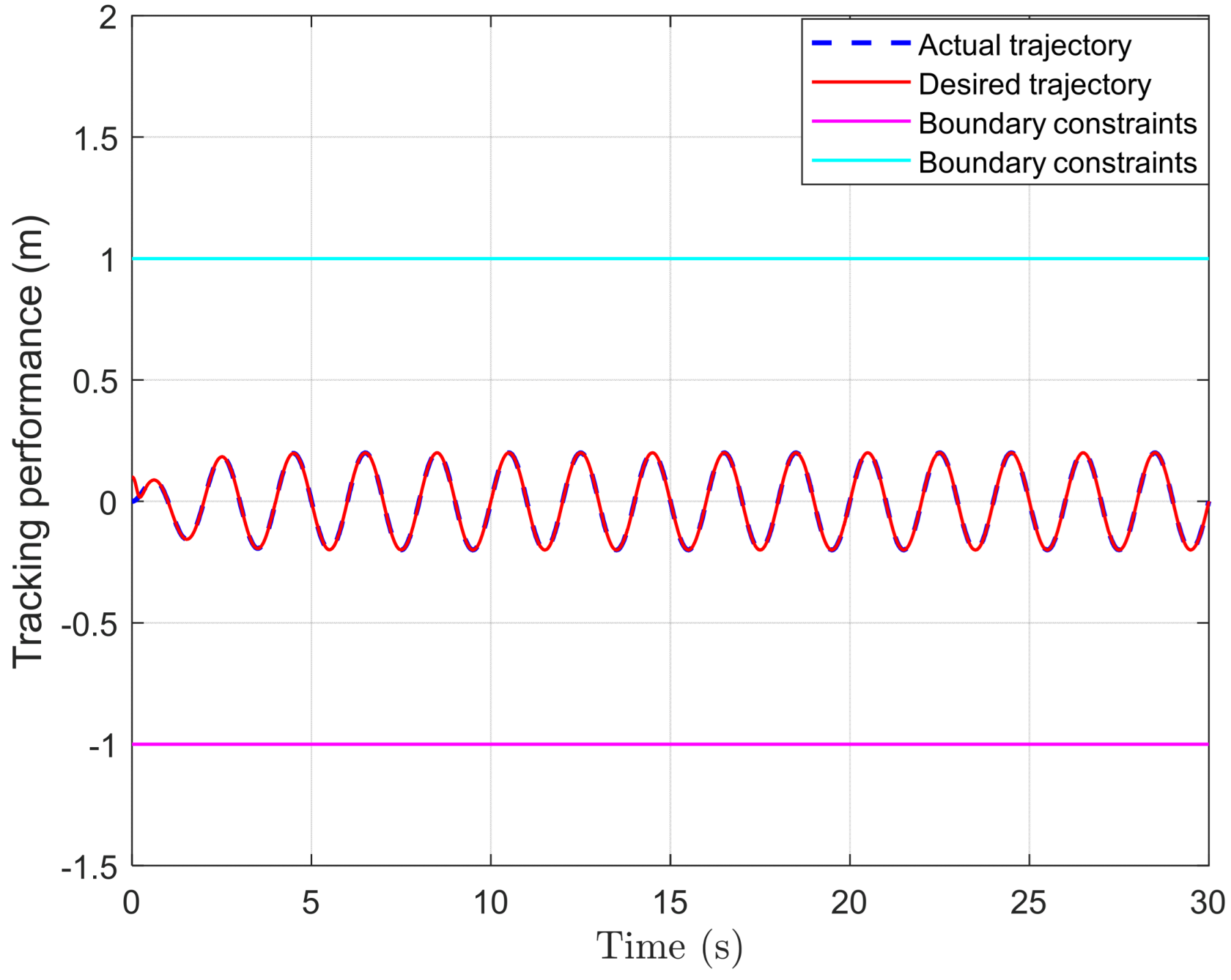
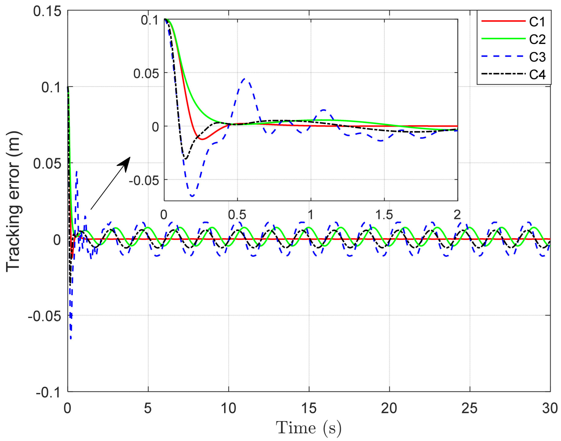
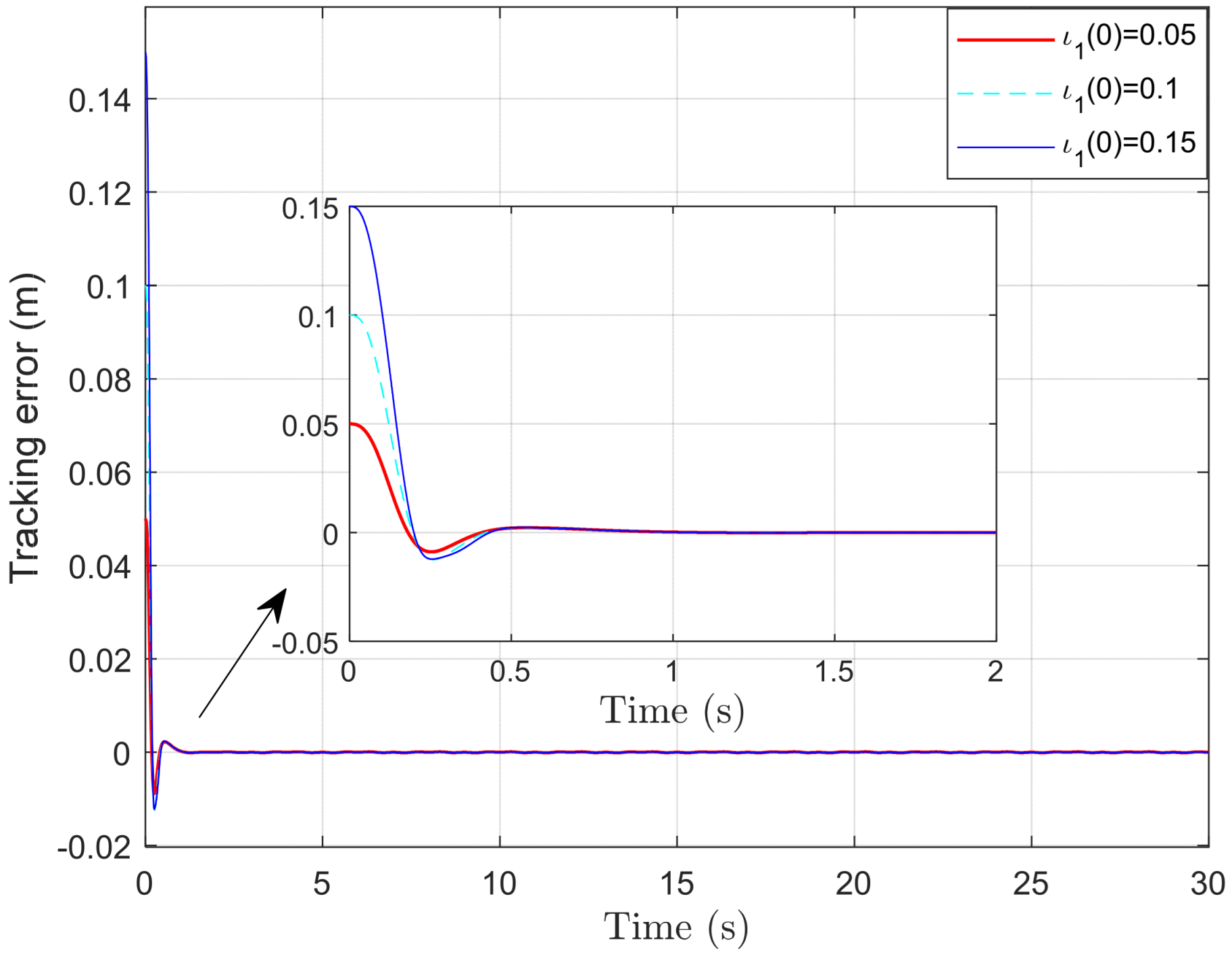
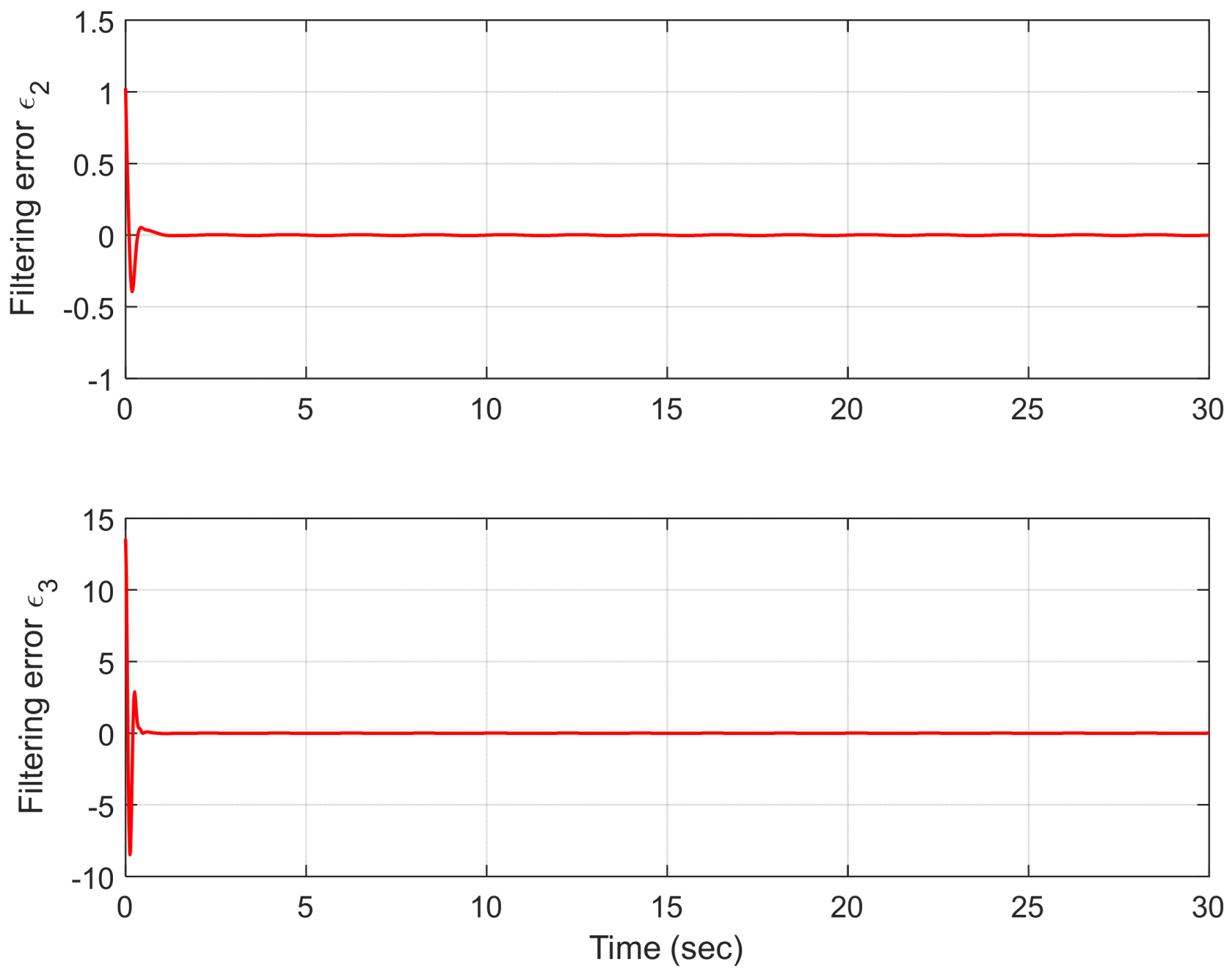
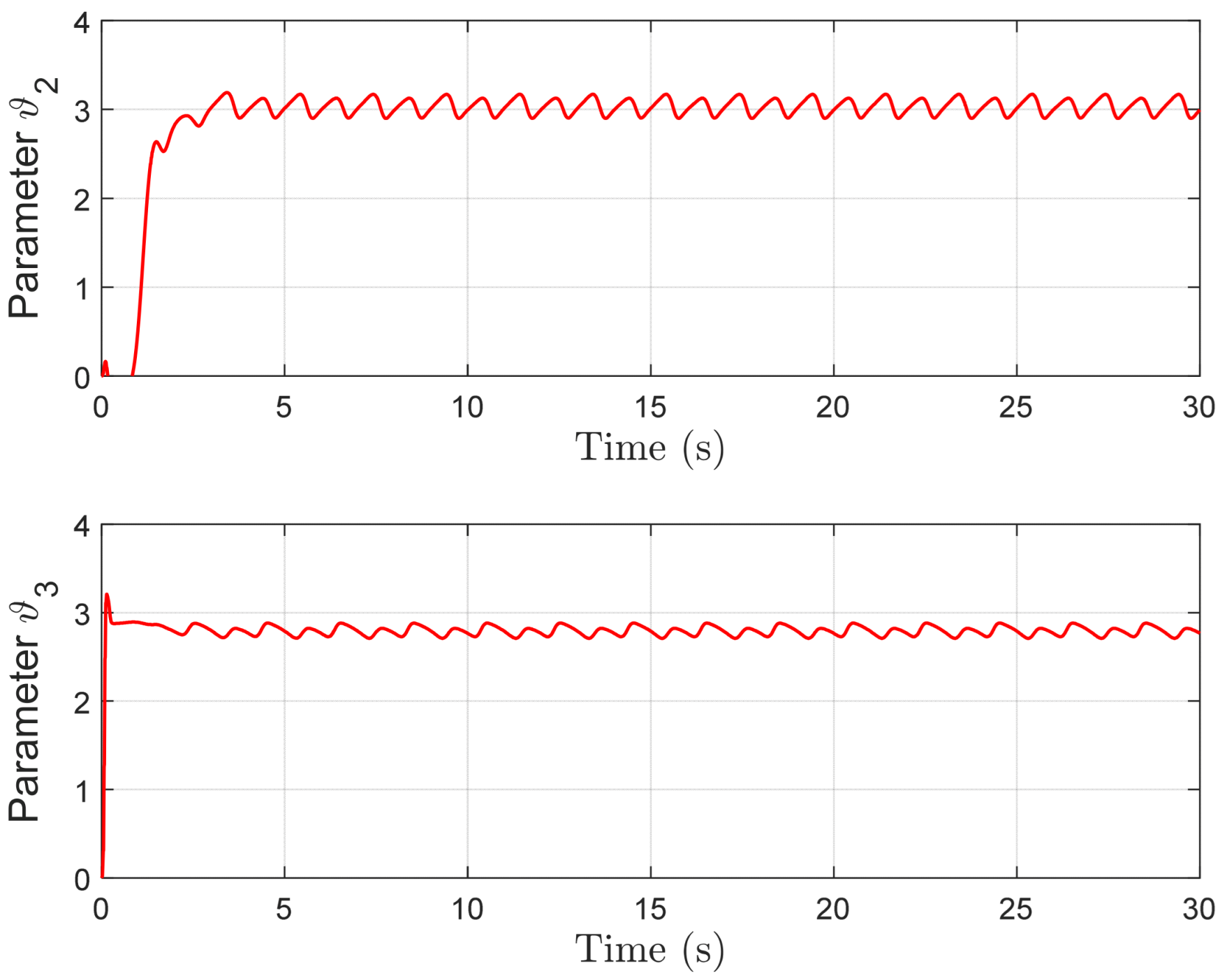
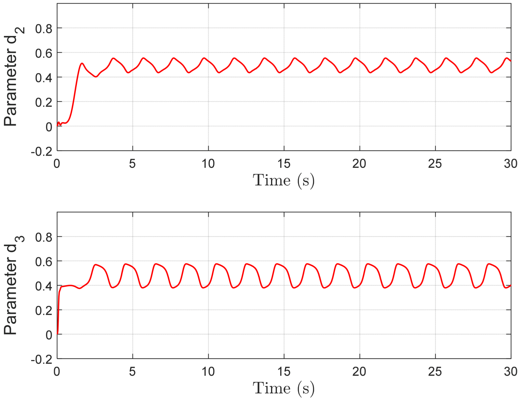
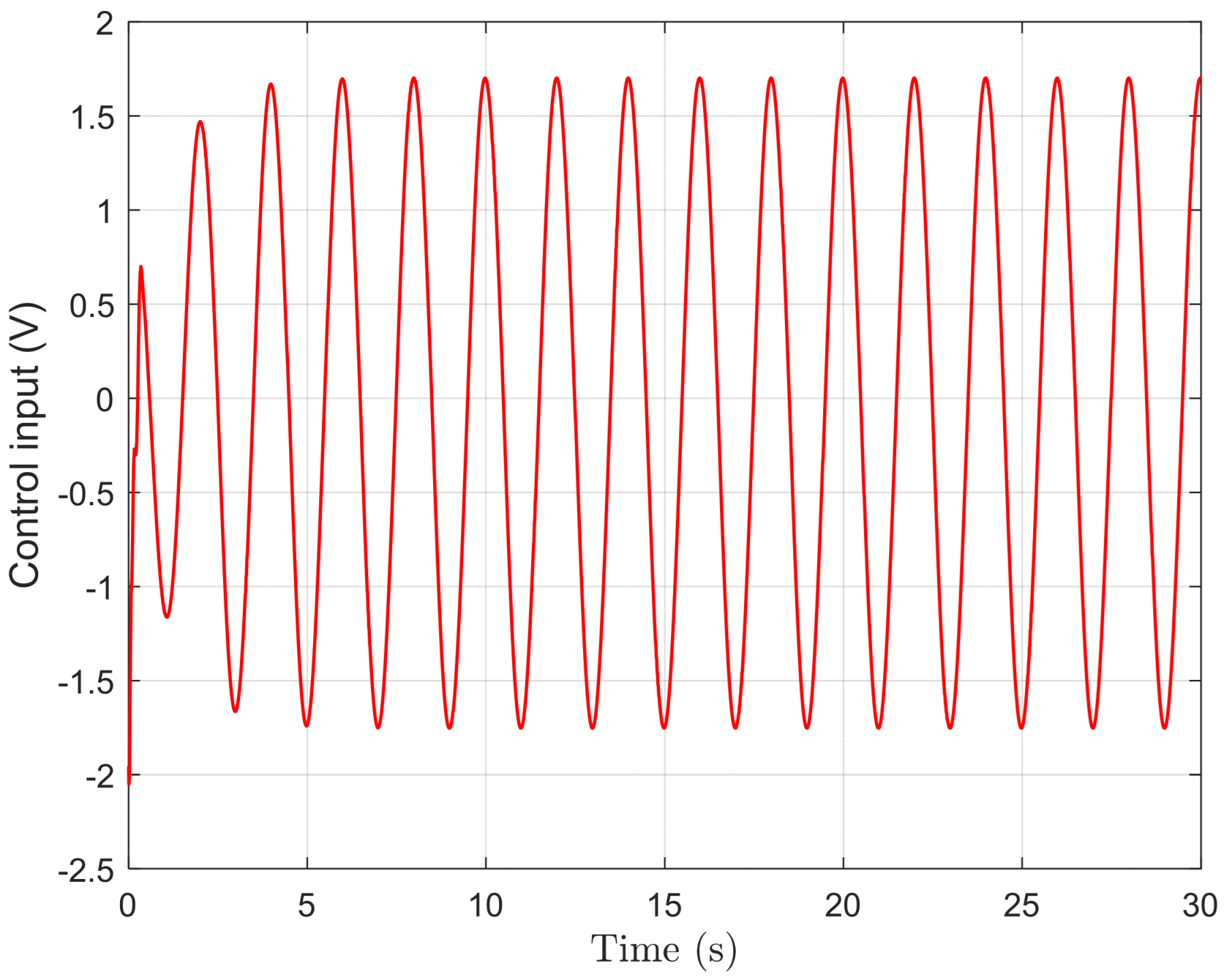
Figure 2 illustrates the tracking performance of the proposed controller under predefined boundaries. As observed, the developed scheme exhibits superior control performance: the system output is strictly maintained within the specific constraints, and the target trajectory is rapidly tracked within the prescribed time. Furthermore, Figure 3 presents the tracking errors of the same hydraulic system following identical trajectories under four different controllers. This comparative analysis further demonstrates the exceptional control capability of the proposed strategy. Figure 4 reveals the control responses under varying initial conditions. It is evident that regardless of the initial states, the tracking errors are uniformly driven into a small bounded region near the origin within the specified timeframe, highlighting the preassigned-time convergence property of the proposed method. Moreover, the trajectories of the filtering errors ${\epsilon }_2$ and ${\epsilon }_3$ under the proposed controller are depicted in Figure 5. These errors successfully converge to a microscopic neighborhood of zero within the prescribed time, verifying the efficacy of the filtering algorithm. Figure 6 and Figure 7 plot the estimation trajectories of the adaptive parameters ${\widehat{\vartheta }}_2$ and ${\widehat{\vartheta }}_3$, and the disturbances ${\widehat{d}}_2$ and ${\widehat{d}}_3$, respectively. Ultimately, all estimated signals are rapidly driven into a bounded neighborhood of their nominal values and maintain dynamic tracking thereafter, further corroborating the validity of the learning mechanisms. Finally, the actual control input of the system is provided in Figure 8.

Case 2.

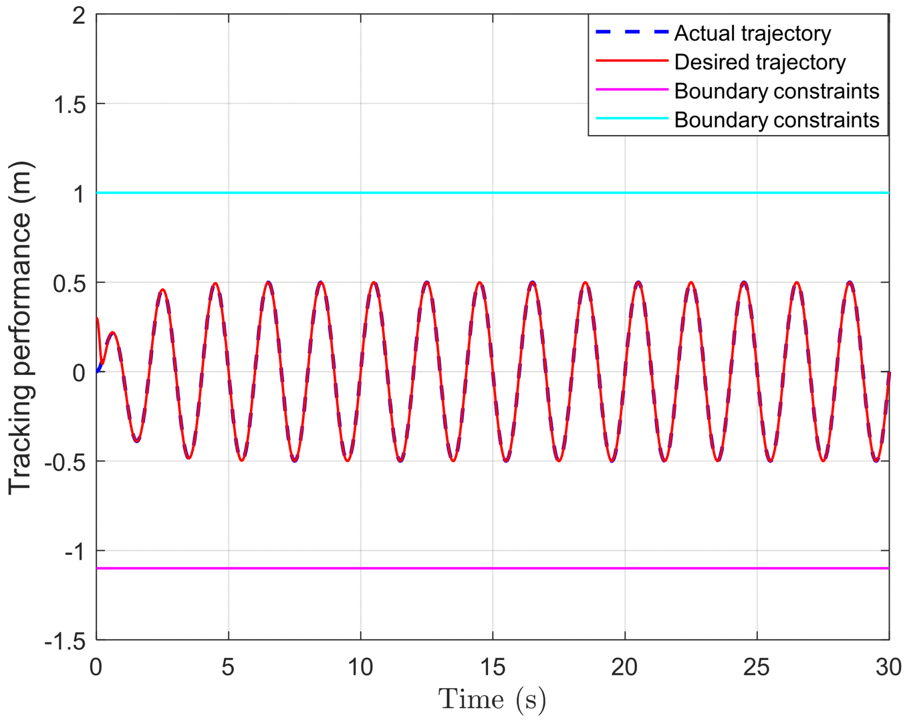
To further verify the control performance of the proposed algorithm, the reference trajectory is modified to  ${\iota }_d=0.5\sin (\pi t)(1-e^{-t})$. Simultaneously, the initial state ${\iota }_1(0)$ is varied, and the asymmetric constraint boundaries are adjusted to  $N_1=1.1$  and  $N_2=1$. All other control parameters remain identical to those in Case 1. The corresponding simulation results are detailed below.

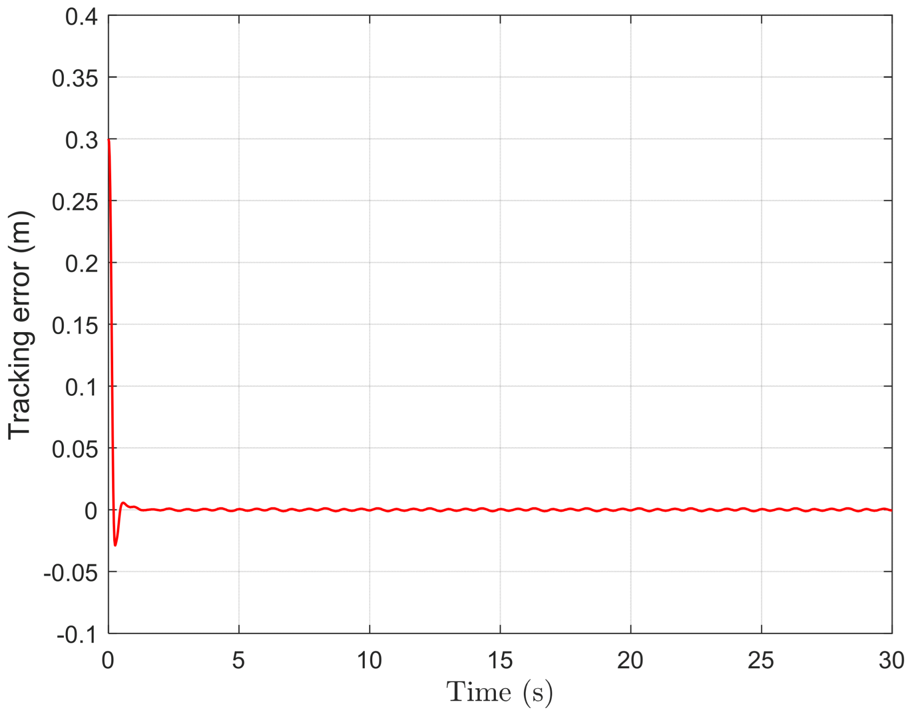
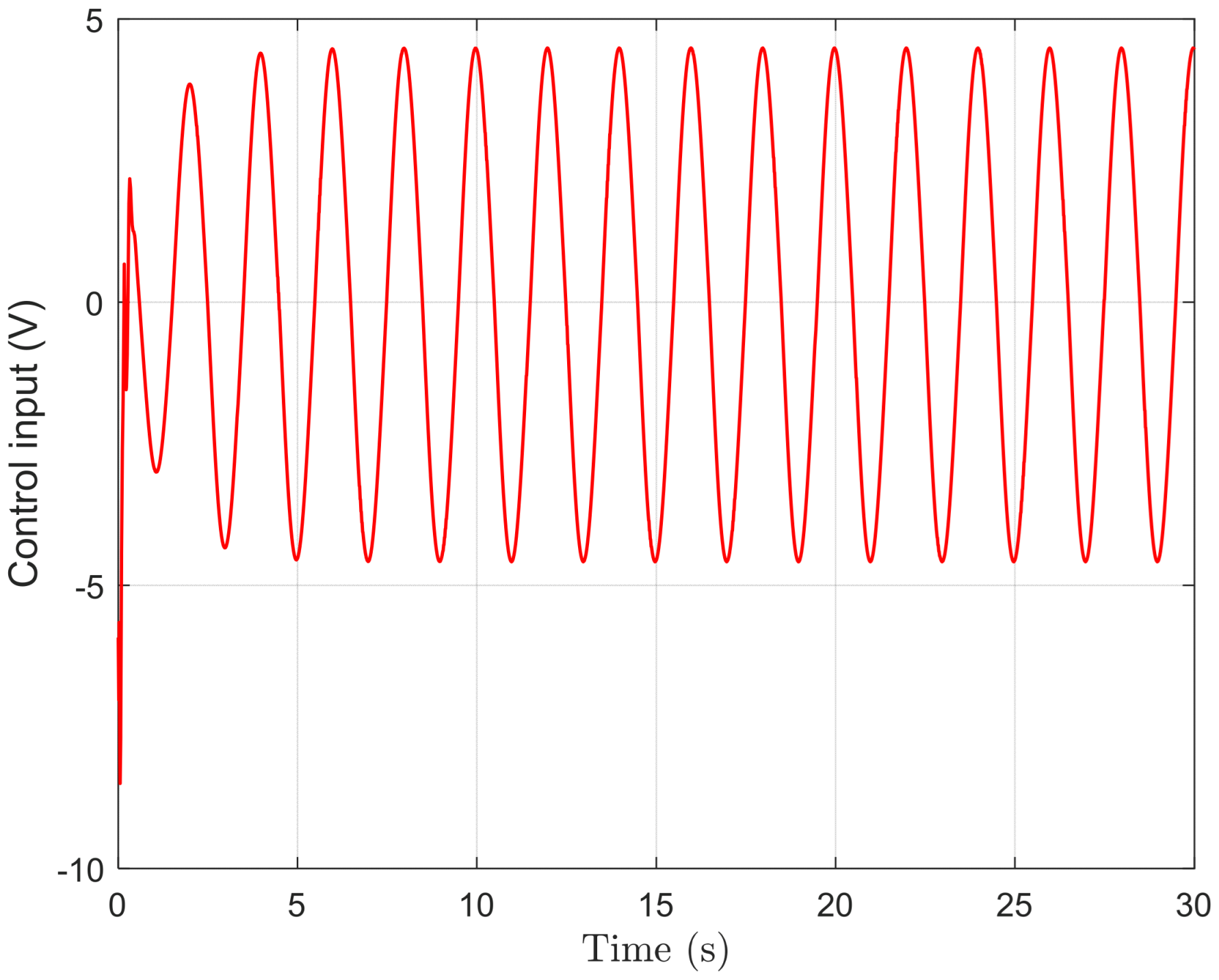
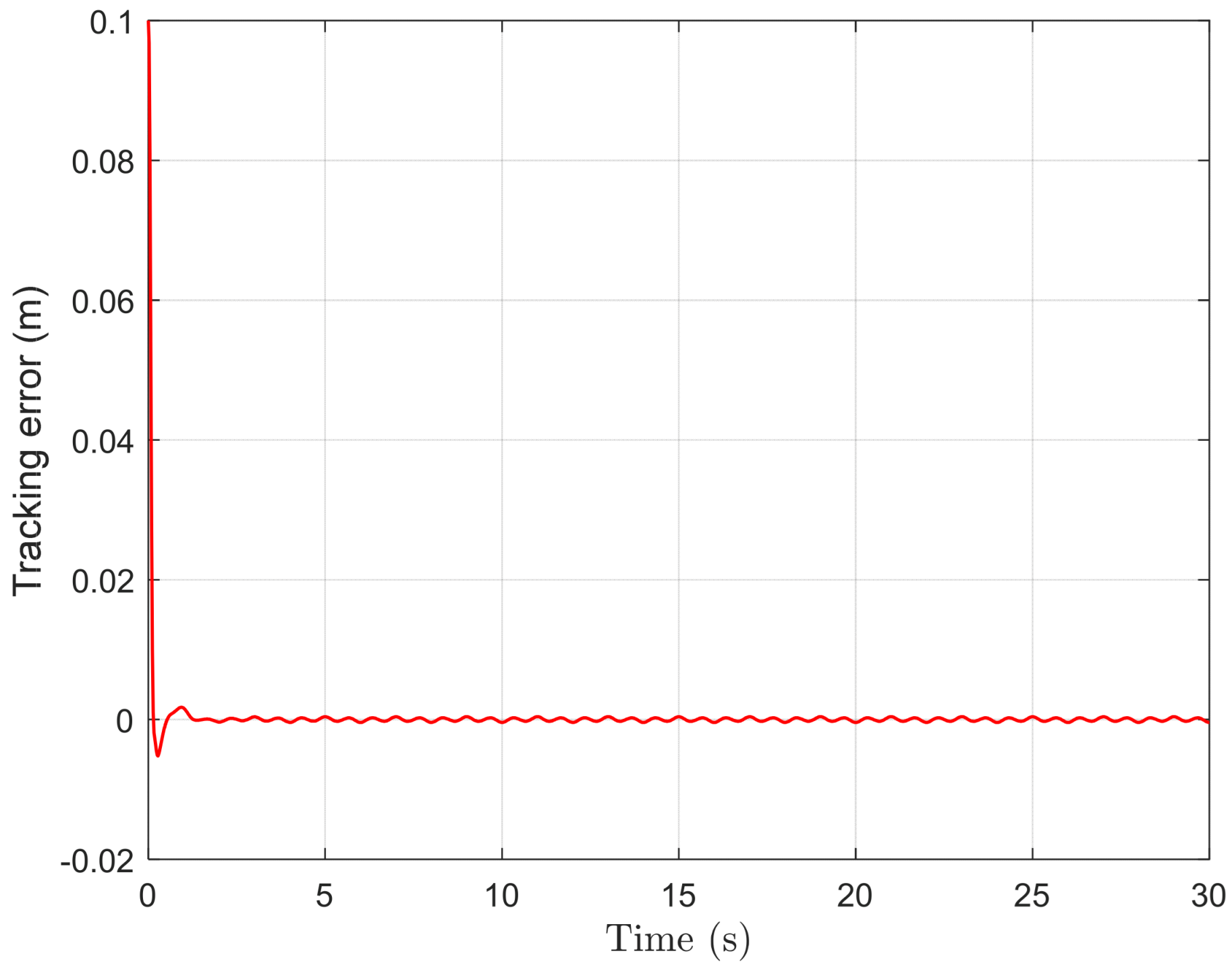
Figure 9 illustrates the dynamic tracking response of the system under the altered operating conditions, demonstrating that the system output is strictly confined within the constraint boundaries while exhibiting excellent tracking performance. The error trajectory depicted in Figure 10 further demonstrates that the tracking error is strictly driven into a small bounded interval near zero within the preassigned time. This comprehensively substantiates the excellent control performance of the proposed algorithm under varying operating conditions. Finally, Figure 11 displays the control input.

Case 3.

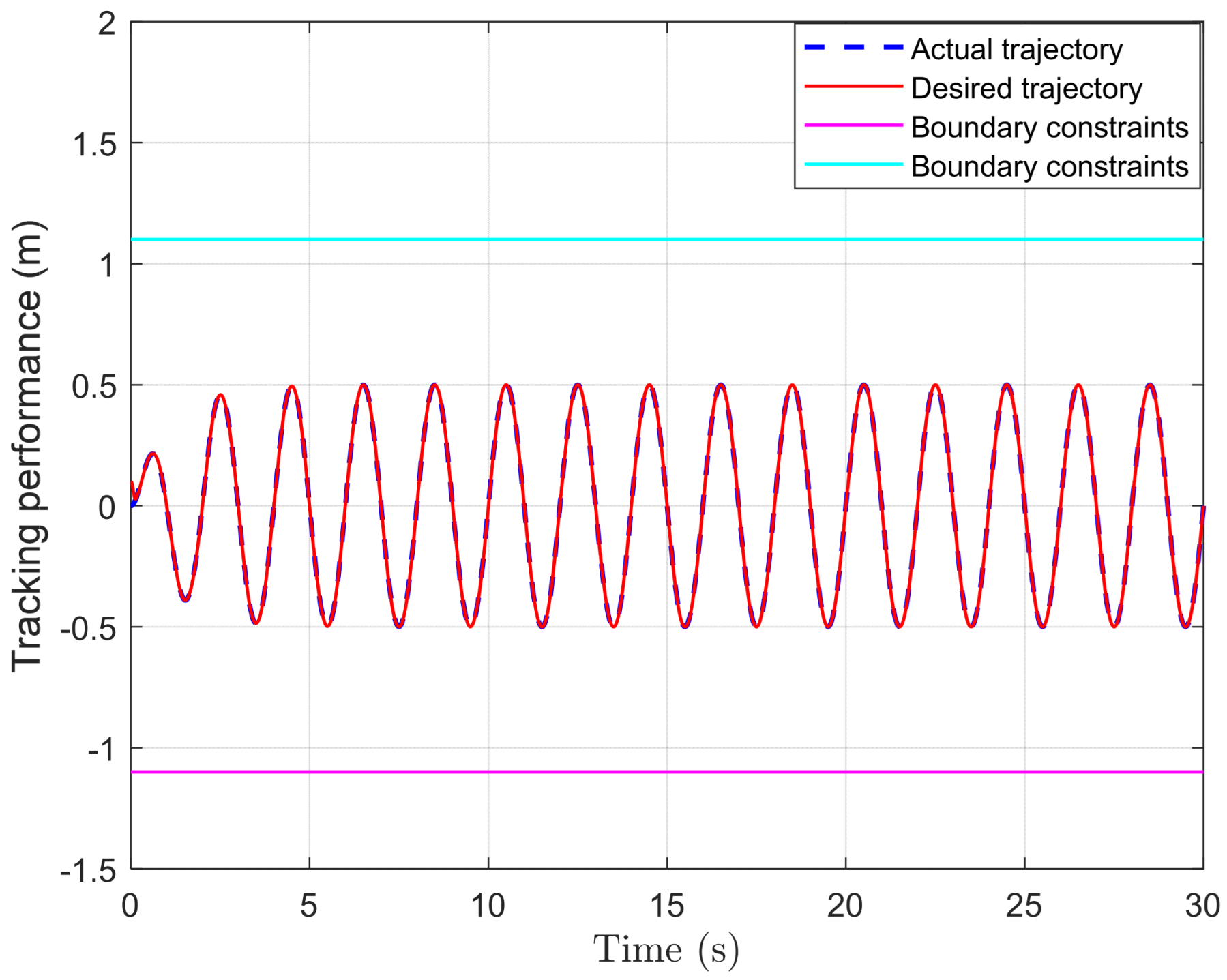
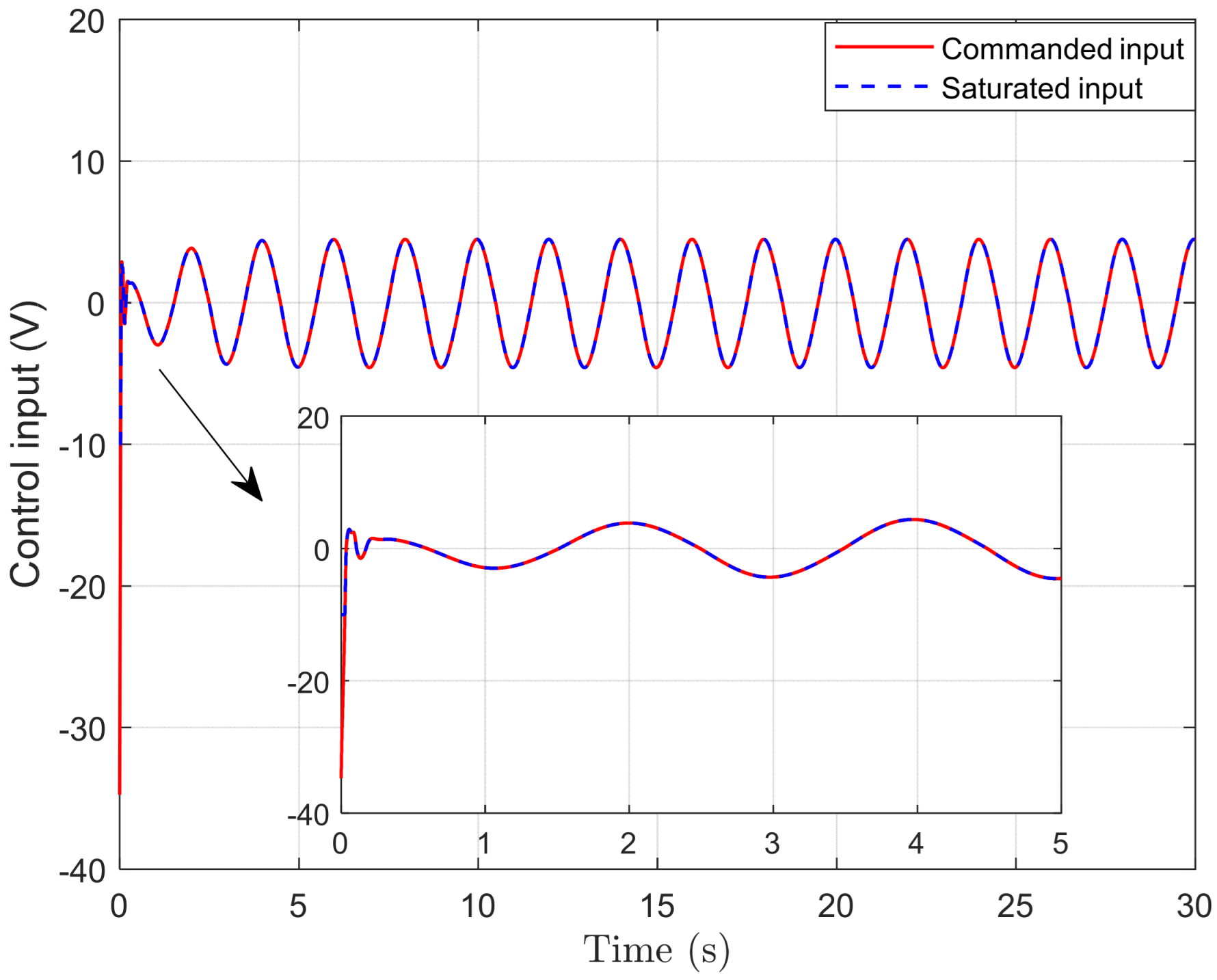
To further verify the effectiveness of the proposed method, actuator saturation is introduced in Case 3. The actuator saturation limits are set to range from −10 V to +10 V. The reference trajectory is modified to  ${\iota }_d=0.5sin\left(\pi t\right)\left(1-e^{\left(-t\right)}\right)$. The controller parameters are set as follows: ${\iota }_1(0)=0.1$, $t_h=1.5$, $\eta =1$, $b_f=0.05$, $m=2$, $n=1$, $k_1=40$, $k_2=70$, $k_3=90$, $N_1=1.1$, $N_2=1.1$, ${\gamma }_{21}=200$, ${\gamma }_{31}=1$, ${\gamma }_{22}=10$, ${\gamma }_{32}=1.5$, ${\omega }_2=80$, and ${\omega }_3=200$.

Figure 12 presents the tracking performance of controller C1 under actuator saturation, while Figure 13 shows the corresponding tracking error. Figure 14 compares the control inputs before and after actuator saturation. Taken together, these results demonstrate that the proposed controller maintains satisfactory practical tracking performance even when the actuator voltage is subject to saturation constraints.

5. Conclusions

In this study, an adaptive prescribed-time tracking control strategy based on dynamic surface control is successfully developed for electro-hydraulic servo systems. By structurally integrating a state-dependent constraint transformation with dynamic surface techniques, the proposed framework fundamentally resolves the restrictive output constraint issues while elegantly bypassing the inherent complexity explosion problem. Furthermore, the synthesis of prescribed-time-driven adaptive mechanisms and smooth robust terms enables the system to actively learn nominal parametric deviations and effectively compensate for time-varying uncertainties. Rigorous Lyapunov analysis validates that the synthesized controller strictly prevents constraint violation throughout the entire operation. More importantly, it guarantees that the tracking errors are forcibly driven into a microscopic neighborhood of the origin within a user-designated settling time. Despite these advancements, a recognized limitation of the current method is its confinement to constant constraint boundaries. Consequently, future research endeavors will focus on extending this framework to accommodate time-varying asymmetric output constraints and further enhancing the ultimate tracking precision, thereby comprehensively safeguarding the operational stability of practical hydraulic systems.

References

1. Yang, H.; Xu, B.; Cheng, M.; Peng, L.; Zhang, J.; Sun, G.; Ding, R. A Review of Independent Metering Control System for Mobile Machinery. Int. J. Hydromechatron. 2025, 8, 1–39. [Google Scholar] [CrossRef] [Scilit]
2. Chen, X.; Tang, Y.; Huang, X.; Wang, W.; Guo, J.; Lin, F.; Jia, L.; Yang, H.; Zhu, Y. Automation and synchronisation on electro-hydraulic lifting system of tunnel boring machine segment assembly. Int. J. Hydromechatron. 2025, 8, 94–120. [Google Scholar] [CrossRef] [Scilit]
3. Cao, X.; Zhao, Z.; Zhu, W.; Lian, G.; Ye, M.; Alam, M.M. Ride comfort analysis of hydro-pneumatic suspension considering variable damping matched with dynamitic load. Int. J. Hydromechatron. 2025, 8, 317–342. [Google Scholar] [CrossRef] [Scilit]
4. Yang, X.; Ge, Y.; Zhu, W.; Deng, W.; Zhao, X.; Yao, J. Adaptive Motion Control for Electro-Hydraulic Servo Systems with Appointed-Time Performance. IEEE/ASME Trans. Mechatron. 2025, 30, 7009–7018. [Google Scholar] [CrossRef] [Scilit]
5. Yang, X.; Deng, W.; Yao, J. Neural Adaptive Dynamic Surface Asymptotic Tracking Control of Hydraulic Manipulators with Guaranteed Transient Performance. IEEE Trans. Neural Netw. Learn. Syst. 2023, 34, 7339–7349. [Google Scholar] [CrossRef] [Scilit] [PubMed]
6. Van, M.; Do, V.-T.; Khyam, M.O.; Do, X.P. Tracking Control of Uncertain Surface Vessels with Global Finite-Time Convergence. Ocean Eng. 2021, 241, 109974. [Google Scholar] [CrossRef] [Scilit]
7. Gao, D.; Dong, Z.; Mao, J.; Liu, L.; Guo, Y. Finite-Time Non-Fragile Performance-Constrained Control for Free-Flying Flexi-ble-Joint Space Robots with Actuator Saturation. Adv. Space Res. 2026, 78, 2827–2842. [Google Scholar] [CrossRef] [Scilit]
8. Hong, Y.; Jiang, Z.-P. Finite-Time Stabilization of Nonlinear Systems with Parametric and Dynamic Uncertainties. IEEE Trans. Autom. Control 2006, 51, 1950–1956. [Google Scholar] [CrossRef] [Scilit]
9. Zhang, C.; Yang, J.; Yan, Y.; Fridman, L.; Li, S. Semiglobal finite-time trajectory tracking realization for disturbed nonlinear systems via higher-order sliding modes. IEEE Trans. Autom. Contr. 2020, 65, 2185–2191. [Google Scholar] [CrossRef] [Scilit]
10. Zuo, Z.; Han, Q.-L.; Ning, B.; Ge, X.; Zhang, X.-M. An Overview of Recent Advances in Fixed-Time Cooperative Control of Multiagent Systems. IEEE Trans. Ind. Inform. 2018, 14, 2322–2334. [Google Scholar] [CrossRef] [Scilit]
11. Wang, Y.; Shen, R.; Zhu, F.; Zhang, C.; Zhao, X. Distributed Fixed-Time Event-Triggered Containment Control for Nonlinear Multiagent Systems with Actuator Faults. J. Frankl. Inst. 2023, 360, 14454–14479. [Google Scholar] [CrossRef] [Scilit]
12. Ma, J.; Sun, H.; Tan, C.; Zhao, T.; Liu, K. Non-Singular Fixed-Time Robust Containment Control for Autonomous Surface Vehicles. Ocean Eng. 2023, 287, 115887. [Google Scholar] [CrossRef] [Scilit]
13. Song, Y.; Wang, Y.; Holloway, J.; Krstic, M. Time-Varying Feedback for Regulation of Normal-Form Nonlinear Systems in Prescribed Finite Time. Automatica 2017, 83, 243–251. [Google Scholar] [CrossRef] [Scilit]
14. Que, N.; Deng, W.; Zhou, N.; Yao, J. Disturbance Observer-Based Prescribed-Time Tracking Control of Nonlinear Systems with Non-Vanishing Uncertainties. IEEE Trans. Circuits Syst. II 2024, 71, 3131–3135. [Google Scholar] [CrossRef] [Scilit]
15. Ye, H.; Song, Y. Prescribed-time tracking control of MIMO nonlinear systems with nonvanishing uncertainties. IEEE Trans. Autom. Contr. 2023, 68, 3664–3671. [Google Scholar] [CrossRef] [Scilit]
16. Tran, D.T.; Truong, H.V.A.; Jin, M.; Ahn, K.K. Finite-Time Output Control for Uncertain Robotic Manipulators with Time-Varying Output Constraints. IEEE Access 2022, 10, 119119–119131. [Google Scholar] [CrossRef] [Scilit]
17. Singh, S.; Kumar, S.R.; Mukherjee, D. Barrier Lyapunov Function Based Impact Time Guidance with Field-of-View and Input Constraints. IFAC-Pap. 2022, 55, 412–417. [Google Scholar] [CrossRef] [Scilit]
18. Li, D.; Chen, C.L.P.; Liu, Y.-J.; Tong, S. Neural Network Controller Design for a Class of Nonlinear Delayed Systems with Time-Varying Full-State Constraints. IEEE Trans. Neural Netw. Learn. Syst. 2019, 30, 2625–2636. [Google Scholar] [CrossRef] [Scilit] [PubMed]
19. Farrell, J.A.; Polycarpou, M.; Sharma, M.; Dong, W. Command Filtered Backstepping. IEEE Trans. Autom. Control 2009, 54, 1391–1395. [Google Scholar] [CrossRef] [Scilit]
20. Zhao, K.; Song, Y.; Zhang, Z. Tracking control of MIMO nonlinear systems under full-state constraints: A Single-parameter adaptation approach free from feasibility conditions. Automatica 2019, 107, 52–60. [Google Scholar] [CrossRef] [Scilit]
21. Wang, H.; Meng, Z.; Ma, J.; Zhao, X. Adaptive Fixed-Time Dynamic Surface Tracking Control for High-Order Non-strict-Feedback Nonlinear Switched Systems. Neurocomputing 2024, 589, 127590. [Google Scholar] [CrossRef] [Scilit]
22. Chen, K.; Astolfi, A. Adaptive Control for Systems with Time-Varying Parameters. IEEE Trans. Autom. Control 2021, 66, 1986–2001. [Google Scholar] [CrossRef] [Scilit]
23. Ma, Z.; Wang, Q. Adaptive Control of Nonlinear Time-Varying Systems with Unknown Parameters and Model Uncertainties. Aerosp. Sci. Technol. 2024, 155, 109677. [Google Scholar] [CrossRef] [Scilit]
24. Fidan, B.; Zhang, Y.; Ioannou, P.A. Adaptive Control of a Class of Slowly Time Varying Systems with Modeling Uncertainties. IEEE Trans. Autom. Control 2005, 50, 915–920. [Google Scholar] [CrossRef] [Scilit]
25. Nie, S.-C.; Qian, L.-F.; Chen, L.-M.; Tian, L.-F.; Zou, Q. Barrier Lyapunov Functions-Based Dynamic Surface Control with Tracking Error Constraints for Ammunition Manipulator Electro-Hydraulic System. Def. Technol. 2021, 17, 836–845. [Google Scholar] [CrossRef] [Scilit]
Figure 1. Simplified model of the hydraulic servo system.
Symmetry 18 01397 g001
Figure 2. Tracking performance of C1 in Case 1.
Symmetry 18 01397 g002
Figure 3. Tracking errors of four controllers in Case 1.
Symmetry 18 01397 g003
Figure 4. Tracking errors with different initial conditions in Case 1.
Symmetry 18 01397 g004
Figure 5. Filtering errors ε 2 and ε 3 of C1 in Case 1.
Symmetry 18 01397 g005
Figure 6. Estimation of ϑ 2 and ϑ 3 of C1 in Case 1.
Symmetry 18 01397 g006
Figure 7. Estimation of d 2 and d 3 of C1 in Case 1.
Symmetry 18 01397 g007
Figure 8. Control input of C1 in Case 1.
Symmetry 18 01397 g008
Figure 9. Tracking performance of C1 in Case 2.
Symmetry 18 01397 g009
Figure 10. Tracking error of C1 in Case 2.
Symmetry 18 01397 g010
Figure 11. Control input of C1 in Case 2.
Symmetry 18 01397 g011
Figure 12. Tracking performance of C1 in Case 3.
Symmetry 18 01397 g012
Figure 13. Tracking error of C1 in Case 3.
Symmetry 18 01397 g013
Figure 14. Control input of C1 in Case 3.
Symmetry 18 01397 g014