Symmetry-Guided Neural Approximation and Convolutional Non-Dominated Sorting on Synthetic Two-Objective Benchmarks Toward Option-Pricing Model Research in Financial Mathematics and Quantitative Economic Analysis

Abstract

Two-objective optimization requires both reliable front approximation and explainable non-dominated extraction. This study develops a theoretical and computational method that maps sampled objective vectors to rasterized objective-space images and processes their Pareto structure through supervised neural approximation, a deterministic convolutional extractor, and exploratory reinforcement search. Network I reconstructs a high-density sampled occupancy image from sparse samples, whereas Network II approximates the sampled Pareto-front boundary. The principal algorithmic contribution is a fixed cross-correlation kernel derived from the two-objective dominance quadrant and coupled with a cell archive that preserves original vectors and resolves raster collisions through exact dominance checks. Under the stated coordinate convention, central inversion relates the dominating and dominated displacement quadrants, translation-equivariant cross-correlation applies the same local relation across the grid, and minimization selects only the improvement-directed boundary. Experiments on SCH, FON, POL, KUR, and ZDT synthetic benchmarks assess front-geometry recovery and deterministic extraction on grids from 127 × 127 to 2048 × 2048; the reinforcement-learning results on SCH are interpreted as exploratory feasibility evidence. The present evidence is therefore confined to synthetic benchmarks. The method provides a benchmark-based methodological foundation for future multi-criterion model-selection and calibration research, including option-pricing model research in financial mathematics and quantitative economic analysis.

1. Introduction

Two-objective optimization arises when improving one criterion degrades another, so the solution is a set of non-dominated trade-offs rather than a single scalar optimum. Option-pricing model selection and calibration in financial mathematics and quantitative economic analysis provide one motivating context because pricing fit, parameter stability, hedging robustness, model complexity, and computational cost may conflict. The present article addresses the methodological problem of objective-space approximation and non-dominated extraction. Its experimental evidence is obtained from synthetic benchmark functions, while the financial context identifies the intended direction of subsequent application research [1,2].

Evolutionary multi-objective algorithms, represented by NSGA-II and SPEA2, remain widely used because they maintain candidate populations, rank them through Pareto dominance, and preserve diversity during search [3,4]. Modern implementations, component-wise configuration, decomposition, indicator-based selection, and surrogate-assisted search have improved reliability and sample efficiency [5,6,7,8,9]. Neural approaches can additionally learn preference-conditioned trade-offs, approximate complex Pareto-front geometries, and guide policies through structured decision spaces. These developments are relevant to the present study, but they mainly improve candidate generation, surrogate prediction, or preference-conditioned search, whereas the proposed fixed kernel directly implements a two-objective dominance test after candidate objective vectors have been generated.

Modern toolkits and improved implementations make evolutionary algorithms easier to reproduce, but they do not remove the dependence on population size and repeated dominance checks. Studies on component-wise design and automatic algorithm configuration also show that performance gains increasingly arise from adaptive operators, alternative search structures, and problem-specific computational modules. These results motivate a more structural question: whether dominance itself can be converted into a representation that is easier for deterministic or neural operators to process. If the relation can be expressed in a regular objective-space form, part of the sorting workload can be transferred from nested vector comparison to matrix operations that are naturally parallel.

Surrogate-assisted and Bayesian methods reduce the cost of expensive objective evaluations through learned response models and acquisition functions. In particular, parallel Bayesian optimization of multiple noisy objectives can improve sampling efficiency by selecting candidate evaluations according to expected hypervolume improvement [10]. Its principal mechanism nevertheless remains search and candidate selection rather than a direct reformulation of non-dominated sorting as a regular operation on a dense two-dimensional objective-space image.

Image representations have previously been used to visualize high-dimensional optimization states and to connect optimization trajectories with standard image-processing tools. Encoder-decoder and progressive feature-enhancement models further show how local boundaries and small structures can be preserved in high-resolution images. The present formulation differs in both the represented quantity and the operator: pixels encode occupied cells in a two-objective value plane, and the deterministic kernel is derived from Pareto dominance rather than learned as a generic segmentation filter. The supervised CNN remains an approximation module, while exact non-dominance is supplied only by the rule-based extractor together with the original-vector archive.

Recent application-oriented research illustrates the broader value of combining structured numerical models, multidimensional representations, information fusion, and data-adaptive computation. Interaction-aware robotic intervention, engineering-drawing information protection, multilevel particle-morphology simulation, geometry–intensity sensor calibration, agent-based spatial modelling, and interface-sensitive tomographic reconstruction all rely on the coordinated processing of explicit structural information and complex observational data [11,12,13,14,15,16]. Related developments include reduced-order projection models, multisource state-space prediction, multimodal system-state estimation, precise integration methods, collaborative routing optimization, and multivariate index construction [17,18,19,20,21,22]. Image restoration under rotational motion, discrete-element and finite-element analysis, machine-learning-based industrial detection, high-precision synchronization, and nonlinear structural shape-finding further demonstrate how physical constraints, geometric representations, and computational estimation can be organized within unified numerical frameworks [23,24,25,26,27,28].

A parallel methodological trend concerns the use of surrogate modelling, enhanced neural representations, interpretable learning, and secure intelligent computation. Hierarchical clustering weighted Gaussian-process regression provides a data-efficient approach to low-fidelity prediction, while neural-observer-based Mamba architectures, enhanced visual detection networks, interpretable ensemble models, AI-governance frameworks, and time–frequency deep learning demonstrate complementary strategies for representation learning, prediction, and model control [29,30,31,32,33,34]. Interpretable machine learning for material design, dynamic security computation, intelligent design automation, and learnable-parameter-driven Transformer models further show how structural constraints and adaptive models can be integrated in complex decision environments [35,36,37,38]. Neural-network-supported brain–computer-interface analysis, secure trajectory prediction and task offloading, data-science-assisted multi-criterion material optimization, and autonomous online-learning generation additionally highlight the importance of reliability, feature representation, and adaptive decision mechanisms in intelligent systems [39,40,41,42,43]. Although these studies address different application domains, they collectively support the methodological premise that explicit structural knowledge and nonparametric learning can serve as complementary computational layers.

Symmetry is used here only as an interpretive device for the fixed two-objective operator. For a displacement δ = (δ₁, δ₂), the elementary central inversion J(δ) = −δ maps the local dominating quadrant to the opposite dominated quadrant, while repeated cross-correlation translates the same relation across the grid. Minimization is directional and asymmetric because only simultaneous objective improvement is tested for exclusion. This manuscript therefore does not claim a new symmetry theorem or global invariance of the optimization problem, neural architecture, or Pareto front.

These strands leave a specific computational gap. Existing optimizers primarily determine where candidate vectors should be evaluated, learned front models approximate trade-off sets, and image models provide spatial feature extraction. They do not, in general, convert the two-objective partial order itself into a fixed, explainable grid operator. This study therefore separates three roles: sampled front-image approximation, deterministic dominance extraction, and exploratory decision-space movement. The modules share an objective-space representation and may be combined, but they can also be invoked independently.

Reinforcement learning provides a complementary search mechanism. Value-based and policy-gradient methods can learn sequential decisions under sparse and delayed feedback [44,45]. Multi-objective reinforcement learning further considers vector rewards, coverage sets, preference-conditioned policies, and decomposition-based formulations [46,47,48,49,50,51,52,53,54,55]. For numerical multi-objective programming, the main difficulty is reward sparsity: only a small fraction of transitions improves the maintained non-dominated structure.

The contributions are fourfold. First, this study defines a modular two-objective representation in which sampled objective vectors are mapped to occupancy images without scalarizing the trade-off set; this representation is motivated by future model-selection and calibration research, including option-pricing applications. Second, a cell archive stores each sample index, decision vector, and original objective vector assigned to an occupied raster cell, thereby separating cell-level image processing from exact vector-level reporting. Third, a deterministic cross-correlation extractor is constructed from the two-objective dominance quadrant and equipped with an explicit coordinate convention, finite-range coverage condition, and archive refinement. Fourth, the supervised CNN and the three reinforcement-learning variants are positioned as optional approximation or exploration modules, and the evaluation distinguishes front-image approximation, deterministic extraction, and SCH feasibility evidence rather than combining them into a single competitive claim.

2. Two-Objective Foundations and Local-Symmetry Interpretation

2.1. Generic Two-Objective Formulation and Prospective Option-Pricing Interpretation

In the generic formulation, x may represent model parameters, hyperparameters, or other decision controls. In future option-pricing research, x could collect coefficients of a parametric pricing model together with controls of a nonparametric residual module, while paired objectives could represent pricing fit and stability or complexity, or calibration error and hedging error. In the present benchmark study, however, the objective mapping f is instantiated by synthetic two-objective functions so that the computational behavior of the proposed representation and extraction method can be examined independently of a particular market model.

minimize_x∈X f(x) : = [f₁(x), f₂(x), …, f_m(x)]^⊤,  subject to g_r(x) ≤ 0 (r = 1, …, p).

(1)

Here X ⊆ ℝⁿ, Y ⊆ ℝ^m, f : X → Y, and g : X → ℝ^p. Each feasible vector is mapped to y = f(x). A scalarization can return a single preferred solution, but a full Pareto front normally requires repeated scalar problems. The present framework keeps the vector form and processes the front directly in objective space.

The complete construction is restricted to two objectives and box-constrained decision variables. This scope is not merely an implementation choice: the binary image, the opposite-quadrant dominance relation, and the fixed two-dimensional kernel all depend on a planar objective space. Problems with three or more objectives would require a tensor grid, projection, or graph-based dominance representation and are outside the validated scope of this article.

The resulting numerical pipeline is therefore a general computational layer: feasible samples are drawn from X, mapped by f, encoded as occupied cells, and processed in objective space. A future financial implementation would replace the benchmark mapping with a specified pricing or calibration model while retaining the same distinction between candidate generation, raster representation, cell-level extraction, and vector-level archive refinement.

2.2. Pareto Dominance, Non-Dominated Set, and Pareto Front

For minimization, vector x^a dominates vector x^b only if it is no worse in every objective and strictly better in at least one objective:

x^a ≺ x^b ⇔ [∀i, f_i(x^a) ≤ f_i(x^b)] ∧ [∃j, f_j(x^a) < f_j(x^b)].

(2)

The notation x^a ≺ x^b means that x^a dominates x^b. This relation is a partial order. Many feasible solutions are incomparable because one solution may improve one objective while worsening another, which is the central difference from scalar optimization.

Given a finite or sampled feasible set D ⊆ X, a vector x* ∈ D is dominated if another vector x ∈ D satisfies x ≺ x*. Otherwise, x* is non-dominated. The non-dominated set of the full feasible space is the Pareto set PS, and its image in objective space is the Pareto front PF:

PS : = {x ∈ X : ¬∃z ∈ X such that z ≺ x},   PF : = f(PS).

(3)

This study focuses on PF because the convolutional modules operate in objective space. The associated decision vectors can be recovered through the sample-index mapping used during image construction. This separation clarifies two tasks that are often coupled in evolutionary algorithms: decision-space search and objective-space sorting.

2.3. Objective-Space Imaging and Dominance Symmetry

For two-objective minimization, the objective-space image is a finite occupancy representation of sampled objective vectors. A cell value of one means that at least one vector falls within the cell bounds. The image is not the continuous set f(X), and it becomes meaningful only together with the objective bounds, resolution, sampling density, and the archive described below.

Rasterization is many-to-one. Each occupied cell therefore stores not only a binary value, but also an archive of all original sample indices and objective vectors assigned to that cell. The binary extractor returns a cell-level non-dominated boundary. Before vector-level solutions are reported, the archived vectors in retained boundary cells are checked by the exact Pareto relation, and duplicate or mutually dominated vectors are removed. Without this archive refinement, two distinct samples colliding in one pixel would be indistinguishable and the binary result could only be interpreted as a quantized cell-level approximation.

Quantization error is controlled by the cell widths h₁ and h₂. If a cell center represents all vectors assigned to that cell, the coordinate-wise and Euclidean positional bounds are given in Equation (A2). Lower resolution increases this bound and increases the probability of collisions; higher resolution reduces positional error but increases grid memory, convolution cost, and the sampling density required to occupy the front continuously. The revised claims therefore distinguish the exact sampled vectors, the rasterized cell approximation, and the theoretical continuous Pareto front.

For a displacement δ from an occupied cell, define Q⁻ as the simultaneous-improvement quadrant and Q⁺ as the simultaneous-worsening quadrant. The central inversion J in Equation (A3) maps Q⁻ to Q⁺. This is the local dominance symmetry used to construct the kernel. The cross-correlation operator is translation equivariant because translating the occupancy image translates the response by the same amount. The asymmetric step is the minimization-directed decision rule: only occupancy in Q⁻ invalidates a candidate, so J is not imposed as an invariance of the final output.

y* ≺ y ⇔ y − y* ∈ ℝ₊²∖{0};   y ≺ y* ⇔ y* − y ∈ ℝ₊²∖{0}.

(4)

Equation (7) and the fixed kernel implement this convention. A retained cell has no occupied cell in the simultaneous-improvement quadrant. Other visible external boundaries are not Pareto-optimal under minimization, so the operator uses the local opposite-quadrant relation but keeps only the direction selected by the partial order.

Repeated cross-correlation expands the inspected simultaneous-improvement quadrant. The operation converts cell-level dominance testing into regular image filtering; exact vector-level output is obtained only after archive refinement.

2.4. Neural Computation Modules Used in This Study

The framework uses only the neural operations required by the proposed algorithms: affine layers, two-dimensional convolution, transposed convolution or up-sampling, back-propagation, and value or policy approximation for reinforcement learning. A fully connected layer is written as

h = σ(Wx + b).

(5)

where W is the weight matrix, b is the bias, σ is the activation function, and h is the output. The supervised solver mainly relies on two-dimensional convolution over binary images:

B = f_conv(A,K) = A × K,   b_ij = ∑_{r = 0}^R−1 ∑_{s = 0}^S−1 k_rsa_i+r,j+s.

(6)

Deep-learning libraries implement two-dimensional cross-correlation, commonly named “convolution” in software interfaces. To avoid a notation conflict, f_conv denotes this cross-correlation convention throughout Equations (6), (9) and (10): the kernel is translated without spatial reversal. Network I reconstructs a high-density sampled objective-space image, whereas Network II approximates its Pareto-front boundary.

The reinforcement-learning modules approximate either an action-value function or an Actor-Critic pair. Their states, actions, and rewards are defined from decision variables, dominance updates, and objective-space images, not from generic image labels.

2.5. Implementation Environment

The implementation uses Python 3.8.10 using TensorFlow 2.8.0, NumPy 1.21.6, SciPy 1.7.3, and Matplotlib 3.5.1. TensorFlow provides neural training and inference, while NumPy/SciPy support sampling and benchmark evaluation. The convolutional components are compatible with GPU execution.

Experiments were run on a Dell Precision 7530 mobile workstation with an Intel Core i7-8750H CPU, 16 GB RAM, and an Nvidia Quadro P3200M GPU. The hardware description contextualizes the archived runtime values. The revised evaluation reports method-specific evidence and does not use these results to rank independently tuned optimization algorithms.

3. Proposed Modular Two-Objective Computational Method

3.1. Nonparametric CNN Mapping from Objective-Space Images to Pareto-Front Approximations

The nonparametric component casts Pareto-front approximation as image-to-image prediction. For each benchmark instance, decision vectors are sampled uniformly from the decision box, evaluated by the explicit objective functions, and rasterized as a sparse binary occupancy image. In an option-pricing application, these explicit objectives would be supplied by a parametric or hybrid calibration model. A substantially larger finite sample of the same mapping provides a high-density sampled objective-space approximation, from which the sampled Pareto-front label is constructed. Neither target is an exact continuous image of f(X); both depend on the retained objective bounds, sample count, and raster resolution.

Two encoder-decoder CNNs are used. Network I maps a sparse objective-space image to a reconstructed full image. Network II maps the full or reconstructed image to a PF image. This design keeps both training and inference in objective space and avoids scalarizing the vector problem. The two-network design also makes the computational roles explicit: reconstruction and PF extraction are separated rather than hidden inside one opaque end-to-end network.

Network I reconstructs the objective-space image from sparse samples. Its stage-wise configuration is summarized in

Table 1. Stage-wise architecture and reconstruction roles of Network I.

Stage	Layer Indices	Operation	Channels	Kernel/Scale	Computational Role
Encoder E1	0–3	3 × Conv2D + MaxPooling2D	32	3 × 3; pool 2 × 2	Local occupancy encoding
Encoder E2	4–7	3 × Conv2D + MaxPooling2D	64	3 × 3; pool 2 × 2	Mid-level spatial encoding
Encoder E3	8–11	3 × Conv2D + MaxPooling2D	128	3 × 3; pool 2 × 2	High-level geometry encoding
Encoder E4	12–15	3 × Conv2D + MaxPooling2D	256	3 × 3; pool 2 × 2	Compressed objective-space representation
Bridge	16–17	Conv2DTranspose + UpSampling2D	256	1 × 1; up 2 × 2	Decoder initialization
Decoder D4	18–20	2 × Conv2DTranspose + UpSampling2D	256	3 × 3; up 2 × 2	Coarse reconstruction
Decoder D3	21–23	2 × Conv2DTranspose + UpSampling2D	128	3 × 3; up 2 × 2	Intermediate reconstruction
Decoder D2	24–26	2 × Conv2DTranspose + UpSampling2D	64	3 × 3; up 2 × 2	Fine reconstruction
Decoder D1	27–28	2 × Conv2DTranspose	32	3 × 3	Local boundary refinement
Output	29	Conv2DTranspose	1	5 × 5	Binary occupancy estimate

. The encoder uses 3 × 3 convolutions and four max-pooling stages, while the decoder restores the resolution through transposed convolution and up-sampling.

Network II extracts the PF from the predicted or true objective-space image. Its compact stage-wise configuration is summarized in

Table 2. Compact stage-wise architecture of Network II.

Stage	Layer Indices	Operation	Channels	Kernel/Scale	Boundary-Extraction Role
Encoder E1	0–3	1 × Conv2D + 2 × Conv2D + MaxPooling2D	64	1 × 1, 3 × 3; pool 2 × 2	Local occupancy filtering
Encoder E2	4–7	1 × Conv2D + 2 × Conv2D + MaxPooling2D	128	1 × 1, 3 × 3; pool 2 × 2	Boundary-context encoding
Bridge	8–9	Conv2DTranspose + UpSampling2D	128	1 × 1; up 2 × 2	Resolution restoration
Decoder	10–12	2 × Conv2DTranspose + UpSampling2D	128	3 × 3; up 2 × 2	Front-localization refinement
Output	13–14	2 × Conv2DTranspose	64 → 1	3 × 3	PF occupancy estimate

. It is shallower than Network I because it isolates a boundary segment rather than reconstructing the full region.

The input representation is a binary occupancy grid in which a cell value of one denotes at least one sampled objective vector. After rasterization, decision coordinates are not fed to the CNN; the networks learn the geometry of the objective-space image. The complete phase-structured procedure for data construction, rasterization, target generation, CNN training, and subsequent inference is summarized in

Table 3. Phase-structured CNN training and inference algorithm.

Phase	Step	Operation
Inputs	—	Decision space X; training-problem count N; sampled-vector count K; parameter domain Ω.
Data construction	1	Initialize containers for sparse images, high-density sampled images, and sampled PF labels.
Data construction	2	For i = 1, …, N, sample benchmark parameter vector αi uniformly from Ω.
Data construction	3	For j = 1, …, K, sample $\hat{x}$ij from X and compute $\hat{y}$ij = fobj($\hat{x}$ij; αi).
Rasterization	4	Encode sampled objective vectors as sparse binary image Ŷi.
Target generation	5	Construct the high-density sampled objective-space approximation Yi at the selected resolution.
Target generation	6	Extract sampled non-dominated boundary label Zi = fND(Yi).
Training	7	Estimate Network I parameters β from paired images (Ŷ, Y).
Training	8	Estimate Network II parameters θ from paired images (Y, Z).
Output	9	Return β and θ for new sparse objective-space images.

.

During inference, Network I reconstructs a high-density sampled objective-space approximation from a sparse image, and Network II outputs a sampled PF image. This module is useful only when the target problem belongs to a structural family represented in training, and when rapid image approximation is more important than a formal dominance guarantee. Exact vector-level use requires the deterministic extractor and archive refinement. Sampling density, resolution, and collisions are therefore part of the approximation error rather than incidental plotting choices.

3.2. Convolutional Non-Dominated Sorting Based on PF Extraction Kernels

The deterministic component accepts a binary occupancy matrix A and its cell archive. Its direct output is a binary matrix B that retains an occupied cell only when no occupied cell in the dominance quadrant invalidates it at the selected resolution. The archive is then used for exact vector-level refinement. Unlike Network II, the kernel weights are not trained; they are constructed from the two-objective partial order, which makes the cell-level decision explainable and independent of the supervised training distribution.

A padding matrix  places A at the center of a larger zero matrix. Under the coordinate convention in Equation (A1), potentially dominating cells have larger row indices and smaller column indices. The fixed kernel places ones in that quadrant, and f_conv translates the kernel without spatial reversal.

The integrated fixed-kernel example is summarized through representative raster coordinates in

Table 4. Representative fixed-kernel front coordinates; raster values are rounded to the nearest occupied cell.

Raster Column j	Theoretical Row i	Predicted Row i	Absolute Cell Difference	Cell-Level Outcome
0	225	226	1	Retained
5	235	236	1	Retained
10	242	243	1	Retained
20	249	248	1	Retained
30	253	252	1	Retained
50	255	255	0	Retained

. Unlike a trainable CNN, this is a feedforward convolutional computation with a fixed kernel. Repetition expands the inspected dominance region until the full image extent is covered.

Let A = (a_ij) be the binary image of a finite objective-vector set S. If α and β are represented by occupied pixels a_p,q and a_r,s, respectively, the image-space dominance condition is

β ≺_pix α ⇔ (r − p ≥ 0) ∧ (q − s ≥ 0) ∧ [(r,s) ≠ (p,q)].

(7)

Equation (7) restates two-objective Pareto dominance under the selected matrix convention. A point that dominates α is no larger in both objective values and therefore falls in the corresponding dominance quadrant.

Let K be a PF extraction kernel of size (2u − 1) × (2u − 1), and let B = f_conv(Â, K). For an occupied pixel a_ij representing α, the kernel response satisfies

b_ij = 𝟙[a_ij = 1] · 𝟙[∑_(r,s)∈Dij a_rs = 0].

(8)

The kernel sums occupied pixels in the dominance quadrant. If only the central pixel contributes, the response equals one and α remains non-dominated. If another occupied pixel appears in that quadrant, the response exceeds one and α is removed after thresholding. The proof is therefore constructive: the value of the convolutional response has a direct dominance meaning, rather than being an empirical score produced by a trained classifier.

A binary cell with value one may contain several distinct objective vectors. Convolution alone cannot compare vectors that collide in the same cell because the occupancy value remains one. The implementation therefore associates every cell with a list of original objective vectors and sample indices. After the convolutional boundary cells are obtained, exact pairwise dominance is applied only to archived vectors associated with those cells and, when adjacent cells share a quantization boundary, to the relevant neighboring archives. The reported vector set is the refined archive result; the unrefined image is explicitly described as a cell-level approximation.

B = f_conv(Â,K) = Â × K,   b_ij = ∑_{p = 1}^2u−1 ∑_{q = 1}^2u−1 â_{i+p−1,j+q−1}k_pq.

(9)

â_ij = {a_{i−k+1,j−k+1}, k ≤ i,j ≤ 2k−1; 0, otherwise},   Â ∈ {0,1}^{(3k−2)×(3k−2)}.

(10)

After each cross-correlation, thresholding suppresses cells whose response shows an additional occupied cell in the improvement quadrant, and intersection with A prevents empty cells from being introduced. The coverage condition in Proposition 1 yields the stopping rule in

Table 5. Phase-based fixed-kernel Pareto-front extraction algorithm.

Phase	Step	Operation
Inputs	—	Binary image A = (aij)k×k; padded matrix Â; kernel K2u−1; 2 ≤ u ≤ k; counter ω = 0.
Initialization	1	Set C0 : = Â.
Range expansion	2–4	Compute Cω+1 : = fconv(Cω,K), increment ω, and stop when ω(u − 1) ≥ k − 1.
Thresholding	5–6	Set C : = Cω and apply Ĉ = 0 for responses > 1 and Ĉ = 1 otherwise.
Occupancy restriction	7	Compute B : = Ĉ ∧ A so that empty cells cannot be introduced.
Output	8	Return B as the cell-level PF image before archive refinement.

. The proof is cell-level; the archive refinement is required for collisions.

The computational work and applicability conditions of this rule-based stage are analyzed in Section 3.4 and Appendix A.2; no asymptotic advantage is inferred from the use of convolution alone.

3.3. Exploratory Reinforcement-Learning Candidate Generation

The third component formulates candidate generation as a Markov decision process. States may be decision vectors, binary codes, or distribution parameters; actions update those states; rewards depend on the maintained non-dominated structure. The RL modules are independent candidate generators. Only MOP-AC-sample necessarily invokes the final convolutional extractor in the archived implementation.

MOP-DQN uses a Q-network to approximate action values. The reward is one when the updated state is not dominated by the current set and zero otherwise. Transitions are stored in a replay queue, and mini-batches update the network through the discounted Bellman target. This design is intentionally simple, so the result should be read as a feasibility test for sparse dominance rewards rather than as a state-of-the-art MORL comparison. The complete phase-based MOP-DQN procedure, including initialization, ε-greedy action selection, state transition, replay-based value learning, and output of the maintained non-dominated set, is summarized in

Table 6. Phase-based MOP-DQN search algorithm.

Phase	Step	Operation
Inputs	—	x0, T, Te, γ, batch size b, replay capacity bmax, ε schedule, Q-network fq, optimizer, fobj, fs, and fr.
Initialization	1	Set S : = ∅, replay queue B : = ∅, x : = x0, and moving reward $\overline{R}$ : = 0.
Action selection	2–3	Update ε; choose a random action with probability ε, otherwise a : = argmax fq(x).
Transition	4–7	Compute $\hat{x}$ = fs(x,a), evaluate fobj($\hat{x}$), update S and reward R, and append (x,$\hat{x}$,a,R) to B.
Value learning	8–9	When |B| ≥ b, sample a mini-batch, form the discounted Bellman target, and minimize squared Q error.
Iteration	10	Set x : = $\hat{x}$ and continue until T steps are completed.
Output	11	Return the maintained non-dominated set S.

.

The SCH configuration uses a three-layer Q-network with two hidden layers of 20 ReLU units and two linear output units. The principal settings are given in Equation (11).

θ_DQN : = (x₀,T,T_e,b,b_max,γ,ε₀,ε₁) = (30, 5000, 200, 256, 1000, 0.9, 1, 0.01).

(11)

MOP-AC uses an Actor-Critic structure. The state is a binary code of the decision variable, the Actor outputs action probabilities, and the Critic estimates state value. Equation (12) assigns four ordinal reward levels to repeated, dominated, dominating, and newly non-dominated states. The complete phase-based MOP-AC procedure, including initialization, policy and value evaluation, state transition, temporal-difference updating, and maintenance of the non-dominated set, is summarized in

Table 7. Phase-based MOP-AC search algorithm.

Phase	Step	Operation
Inputs	—	x0, T, γ, Actor fa, Critic fc, optimizer, transition fs, and reward function fr.
Initialization	1	Set S : = ∅, temporary queue B : = ∅, x : = x0, and $\overline{R}$ : = 0.
Policy/value evaluation	2–4	Compute Actor probabilities and Critic value; sample action a from the policy.
Transition	5–7	Compute $\hat{x}$ = fs(x,a), evaluate reward and update S, then compute next-state value $\hat{v}$.
Temporal-difference update	8–11	Update $\overline{R}$, form δ = R − $\overline{R}$ + γ$\hat{v}$ − v, and optimize Actor and Critic losses.
Iteration	12	Set x : = $\hat{x}$ and continue until T steps are completed.
Output	13	Return the maintained non-dominated set S.

.

$$R(x,S)={10}^5\times \{{-10}^{-2},x\in S;{-10}^{-3},\exists \tilde{x}\in S:\tilde{x}\prec x;1,\exists \tilde{x}\in S:x\prec \tilde{x};{10}^{-1},\mathrm{otherwise}\}.$$

(12)

For SCH, both the Actor and the Critic contain two hidden layers with 128 ReLU units. The Actor output has 20 × 2 softmax units because state and action values are represented by 20-bit binary coding. The main settings are given in Equation (13).

θ_AC : = (x₀,T,γ) = (uniform initialization, 5000, 0.99).

(13)

MOP-AC-sample changes the state from a single decision vector to parameters of a normal distribution, including mean and standard deviation. One agent state can therefore generate multiple decision vectors in one step, increasing exploration relative to one-vector updates.

MOP-AC-sample evaluates multiple vectors from one distribution state, rasterizes them into the accumulated occupancy image, and uses newly occupied useful cells as a reward signal. At termination, the fixed extractor and cell archive produce the sampled non-dominated result. This is the only archived branch that directly couples RL and deterministic image extraction. The complete MOP-AC-sample procedure, including distribution-based sampling, occupancy-image updating, Actor–Critic optimization, archive maintenance, and final convolutional extraction, is summarized in

Table 8. Phase-based MOP-AC-sample algorithm.

Phase	Step	Operation
Inputs	—	x0, T, γ, Actor fa, Critic fc, fpf, fobj, fs, and fr.
Initialization	1	Set accumulated image F : = ∅, S : = ∅, queue B : = ∅, x : = x0, and $\overline{R}$ : = 0.
Policy/value evaluation	2–4	Compute Actor probabilities and Critic value, then sample action a.
Distribution sampling	5–8	Decode x as a normal distribution, sample u, evaluate y = fobj(u), rasterize y, and update F : = F ∪ Y.
Transition/reward	9–12	Compute $\hat{\mathrm{x}}$, update reward and S from F, evaluate $\hat{\mathrm{v}}$, update $\overline{\mathrm{R}}$, and form the TD error.
Parameter update	13–14	Update Actor and Critic parameters, set x : = $\hat{x}$, and continue.
Final extraction	15	Apply F : = fpf(F) using the fixed convolutional extractor and archive.
Output	16	Return the PF image F and non-dominated set S.

.

For the SCH trial, the decision space is [−1000, 1000] and the objective-space image resolution is 200 × 200. For one decision variable, the state shape is (s, w + u), where s = 1, w = 20 encodes the mean, and u = 8 encodes the standard deviation. Ten decision vectors are sampled from each decoded state. The main setting is given in Equation (14).

θ_AC-sample : = (x₀,T,γ) = (uniform initialization, 20,000, 0.8).

(14)

3.4. Computational Complexity and Local-Symmetry Interpretation

The framework separates two burdens: decision-space search and objective-space sorting. The supervised CNN handles search indirectly by learning image mappings from sampled data, while the DRL variants search through state transitions. The fixed convolutional extractor addresses sorting once objective vectors have been rasterized.

Let N be the number of sampled vectors. Direct general pairwise dominance checking is O(N²) for two objectives, while specialized two-objective sorting can reach O(N log N). Rasterization costs O(N), and the unoptimized grid operation has work O(Tk²(2u − 1)²), where T is defined above; practical GPU libraries reduce wall-clock time through parallel execution, but do not change the work bound. Storage is O(k² + N) when the occupancy grid and cell archive are both retained. The method therefore has no universal asymptotic advantage over specialized sorting. Its potential benefit is regular parallel filtering when the grid is already available, objective vectors are dense, and sorting rather than objective evaluation is the bottleneck.

The map J is an elementary property of ℝ² and is not claimed as a new mathematical symmetry. Its role is operational: it identifies the opposite local quadrants used to construct the fixed dominance kernel. The methodological contribution lies in encoding that relation as repeated cross-correlation under an explicit raster convention, proving finite-range coverage at the cell level, and recovering exact vector-level output through the cell archive.

The RL modules add reward asymmetry because improvements to the maintained non-dominated structure are intentionally weighted more strongly than repeated or dominated moves. This is a search heuristic, not a symmetry theorem, and its scale robustness is not established by the archived SCH experiment.

3.5. Full Modular Workflow and Cell-Archive Interaction

The architecture is modular rather than a mandatory serial solver. The supervised route maps sparse sampled objective vectors to a reconstructed occupancy image and then to a sampled boundary approximation. The rule-based route accepts candidate vectors from any sampler, evolutionary procedure, or reinforcement-learning agent and applies the fixed extractor directly. MOP-DQN and MOP-AC maintain non-dominated sets internally and do not require a CNN connection, whereas MOP-AC-sample accumulates an occupancy image and invokes the fixed extractor at termination.

During rasterization, each objective vector y = f(x) is assigned to a cell (i, j). The occupancy bit is set to one, while the tuple containing the sample index, x, and y is appended to the corresponding cell archive A_ij. The CNN branches read only the occupancy image. The deterministic branch uses the occupancy map for fixed cross-correlation and then retrieves A_ij from retained cells for exact vector-level dominance refinement.

Table 9. Full modular pipeline, cell-archive construction, and invocation relationships.

Route	Input	Main Operation	Cell Archive and Module Interaction	Output or Next Use
Supervised reconstruction	Sparse sampled occupancy image	Network I reconstructs a high-density sampled occupancy image.	The archive is created during rasterization and preserves original samples; Network I predicts occupancy only.	Reconstructed image passed to Network II or inspected independently.
Supervised boundary approximation	Reconstructed or high-density sampled occupancy image	Network II predicts a sampled Pareto-front boundary.	Predicted cells may be checked against archived vectors through the deterministic route.	Sampled PF image approximation.
Rule-based extraction	Candidate objective vectors from any generator	Rasterization, repeated fixed cross-correlation, thresholding, and intersection with occupied cells.	Each occupied cell stores sample indices and original vectors; retained cells undergo exact dominance refinement.	Cell-level boundary and refined non-dominated vector set.
MOP-DQN	Decision state and replay transitions	Q-value-guided one-state updates.	Maintains a non-dominated set internally; no CNN connection is required.	SCH feasibility candidate set.
MOP-AC	Binary-coded decision state	Actor-Critic one-state updates.	Maintains a non-dominated set internally; no CNN connection is required.	SCH feasibility candidate set.
MOP-AC-sample	Distribution-parameter state	Samples multiple decision vectors and accumulates occupancy.	Creates the cell archive during rasterization and invokes the fixed extractor at termination.	Accumulated image and refined Pareto front.

summarizes the complete data flow, archive construction, and admissible invocation relationships.

Throughout this manuscript, “objective-space occupancy image” denotes the rasterized sampled vectors, “sampled PF image” denotes the CNN boundary approximation, “cell-level boundary” denotes the fixed-kernel output, and “refined non-dominated vector set” denotes the archive-checked result. These terms are used consistently to prevent image approximation from being confused with exact vector-level dominance.

4. Experimental Setup and Evaluation Protocol

4.1. Benchmark Problems and Datasets

The supervised CNN and deterministic extractor are evaluated on two-objective synthetic benchmarks. These functions provide controlled reference geometries for examining front-image approximation, disconnected and nonlinear boundaries, and cell-level extraction. The benchmark role is methodological: the results characterize the proposed representation and operators rather than a market-specific pricing model.

The non-ZDT benchmark families are summarized in

Table 10. Non-ZDT benchmark definitions organized by parameterization and evaluation role.

Family (n)	Parameter/Domain Setting	Objective Mapping	Reference-Front Specification	Geometry Tested
SCH (1)	a, b ∈ [−3, 3], a < b, x ∈ [−3, 3]; SCH: (a, b) = (0, 2)	f1(x) = (x − a)2; f2(x) = (x − b)2	x ∈ [a, b]	Continuous convex front
FON (3)	a ∈ [0.2, 0.8], b ∈ [0.5, 1.5], xi ∈ [−3, 3]; FON uses the standard symmetric diagonal setting	f1(x) = 1 − exp(−b ∑i = 13(xi − a)2); f2(x) = 1 − exp(−b ∑i = 13(xi + a)2)	x1 = x2 = x3 on the diagonal interval of the Pareto set	Symmetric diagonal Pareto set
POL (2)	A1, A2 are fixed trigonometric constants; B1, B2 are trigonometric functions of x1 and x2; xi ∈ [−π, π]	f1(x) = 1 + (A1 − B1)2 + (A2 − B2)2; f2(x) = (x1 + a)2 + (x2 + b)2	Numerical reference PF generated by dense sampling/NSGA-II baseline	Trigonometric irregularity
KUR (3)	xi ∈ [−5, 5]	f1(x) = ∑i= 1n−1 −10 exp(−0.2√(xi2 + xi+12)); f2(x) = ∑i = 1n(|xi|0.8 + 5 sin(xi3))	Numerical reference PF generated by dense sampling/NSGA-II baseline	Nonlinear, non-convex front

. SCH has a continuous convex front, FON has a diagonal Pareto set, POL contains trigonometric components, and KUR produces a nonlinear and non-convex front. These cases test simple, symmetric, and irregular objective-space geometries.

The ZDT-series benchmark definitions and their corresponding geometric characteristics are summarized in

Table 11. ZDT-series benchmark definitions organized by parameterization and evaluation role.

Family (n)	Parameter/Domain Setting	Objective Mapping	Reference-Front Specification	Geometry Tested
ZDT1/ZDT2/ZDT3 generator (30)	a ∈ [0.4, 2.1], b ∈ [0, 12], c ∈ [7, 11], xi ∈ [0, 1]; ZDT1/ZDT2/ZDT3 are generated by specific parameter settings	f1(x) = x1; f2(x) = g(x) [1 − (x1/g(x))a − (x1/g(x)) sin(bπx1)]; g(x) = 1 + c∑i = 2nxi/(n − 1)	x1 ∈ [0, 1], xi = 0 for i = 2, …, n	Convex, concave, and disconnected fronts
ZDT4 (10)	a ∈ [0.3, 2.3], b ∈ [8, 12], c ∈ [3, 5]; ZDT4: (a, b, c) = (0.5, 10, 4); x1 ∈ [0, 1], xi ∈ [−5, 5]	f1(x) = x1; f2(x) = g(x) [1 − (x1/g(x))a]; g(x) = 1 + b(n − 1) + ∑i = 2n[xi2 − b cos(cπxi)]	x1 ∈ [0, 1], xi = 0 for i = 2, …, n	Multimodal decision landscape
ZDT6 (10)	a ∈ [3, 5], b ∈ [2, 6], c ∈ [0.5, 2.5], d ∈ [8, 10], e ∈ [0.2, 0.3]; ZDT6: (a, b, c, d, e) = (4, 4, 2, 9, 0.25)	f1(x) = 1 − sin6(aπx1) exp(−bx1); f2(x) = g(x) [1 − (f1(x)/g(x))c]; g(x) = 1 + d(∑i = 2nxi/(n − 1))e	x1 ∈ [0, 1], xi = 0 for i = 2, …, n	Nonlinear and nonuniform front

. ZDT1, ZDT2, and ZDT3 are generated through a unified parameterized form; ZDT3 provides a disconnected front. ZDT4 introduces multimodality, and ZDT6 has a nonlinear and unevenly distributed front.

The supervised labels are finite sampled approximations. For every problem instance, a sparse sample forms the input occupancy image and a substantially larger sample forms the high-density target occupancy image. The sampled reference front is extracted from the available objective vectors. We therefore refer to each target as a “high-density sampled objective-space approximation” rather than as a complete or exact image of the continuous objective space.

4.2. Training and Inference Protocol for the Supervised CNN Solver

The supervised solver was evaluated as an image-to-image mapping system. A pixel value of one indicates that at least one sampled objective vector falls into the target-space bin; no regression target is assigned to individual decision vectors.

Inference was performed on SCH, FON, POL, KUR, ZDT1, ZDT2, ZDT3, ZDT4, and ZDT6. The CNN output was evaluated against theoretical or high-density sampled reference fronts using Υ and, when applicable, Δ. These metrics characterize the archived front approximation and are not used to rank the method against independently tuned optimizers.

4.3. Evaluation Metrics for PF Approximation

Two indicators were used. The proximity indicator Υ is the mean Euclidean distance from each obtained point to the nearest reference point; a smaller value indicates a closer front:

Υ(P,P*) = |P|⁻¹ ∑_p∈P d(p,P*),   d(p,P*) : = min_q∈P* ‖p − q‖₂.

(15)

For connected fronts, the archived distribution indicator Δ measures adjacent-point spacing and endpoint deviations as defined in Equation (16).

Δ = [d_start + d_end + ∑_i|d_i − đ|]/[d_start + d_end + (|P| − 1)đ].

(16)

The proximity indicator Υ remains the mean nearest-reference distance. The endpoint-based Δ in Equation (16) is interpreted only for a connected front with two well-defined terminal points. ZDT3 contains five disconnected segments, so a single pair of global endpoint penalties does not represent its spacing.

4.4. Experimental Protocol for Convolutional Non-Dominated Sorting

The deterministic extractor was evaluated on 127 × 127, 512 × 512, 1024 × 1024, and 2048 × 2048 binary images, corresponding to 16,129, 262,144, 1,048,576, and 4,194,304 two-dimensional vectors when each pixel is occupied.

The archived implementation used u = 15 for all reported resolutions. This value was not selected by fitting benchmark outcomes. It is an engineering compromise: increasing u reduces T but enlarges the (2u − 1)² kernel footprint and temporary convolution workload, whereas decreasing u produces a smaller kernel but more passes. Because no parameter-sensitivity runs were retained, the revision does not claim that u = 15 is optimal; it is reported as the fixed setting used for the archived runtime measurements. The automatic verification routine performs two exhaustive checks on the finite occupied set. First, for each retained cell, it searches the occupied grid for any cell satisfying Equation (7); a match is recorded as a false retention. Second, for each removed occupied cell, it confirms the existence of at least one dominating occupied cell; failure is recorded as a false removal. The extracted binary boundary is accepted only when both counts are zero and it equals the direct cell-level non-dominated set. The cell archive then applies the original continuous-valued dominance relation within retained boundary archives to remove collision-induced ambiguities.

4.5. Experimental Protocol for MOP-DQN, MOP-AC, and MOP-AC-Sample

The reinforcement-learning experiments are restricted to SCH, a one-variable benchmark with a known convex front. Their purpose is to examine whether the proposed state, action, and dominance-reward definitions can generate a recoverable candidate set. The protocol does not support conclusions for nonlinear, multimodal, disconnected, constrained, or high-dimensional problems.

MOP-DQN uses the network and settings in Equation (11). The decision range is [−30, 30]. Replay learning and an exploration schedule are used to stabilize value estimation.

MOP-AC uses the reward in Equation (12), the settings in Equation (13), and a decision range of [−1000, 1000]. State and action values are represented by 20-bit binary coding.

MOP-AC-sample uses distribution-parameter states and samples ten decision vectors at each step. Its training horizon is T = 20,000 and γ = 0.8, as shown in Equation (14). The final accumulated image is processed by the convolutional PF extractor.

The evaluation is organized by evidence type. The supervised CNN is assessed against theoretical or high-density sampled reference fronts. The fixed extractor is checked against the direct cell-level dominance relation and then refined through the original-vector archive. The reinforcement-learning variants are discussed only as SCH feasibility cases. This separation prevents modules with different computational roles from being treated as one competitive benchmark.

5. Results and Discussion

5.1. Supervised CNN Approximation of Sampled Pareto Fronts

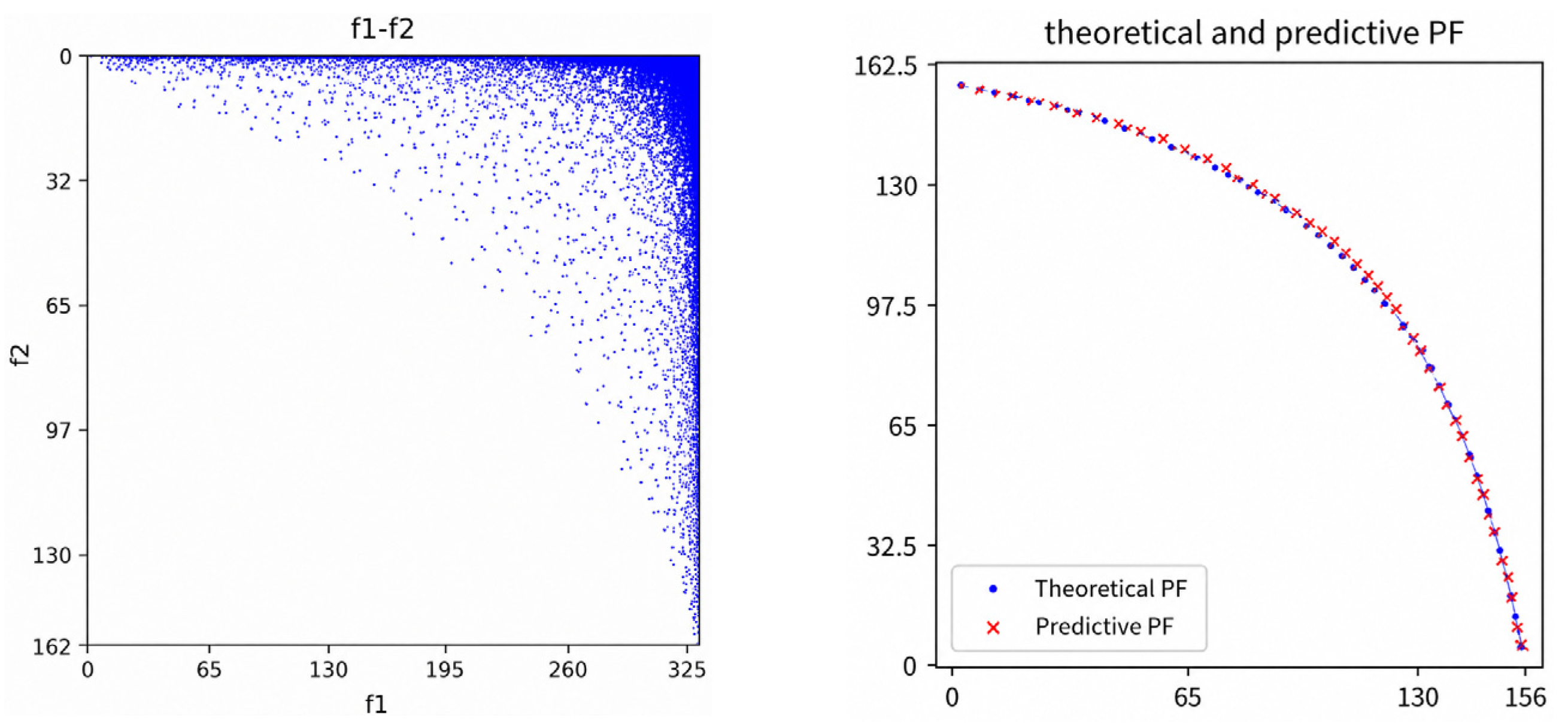
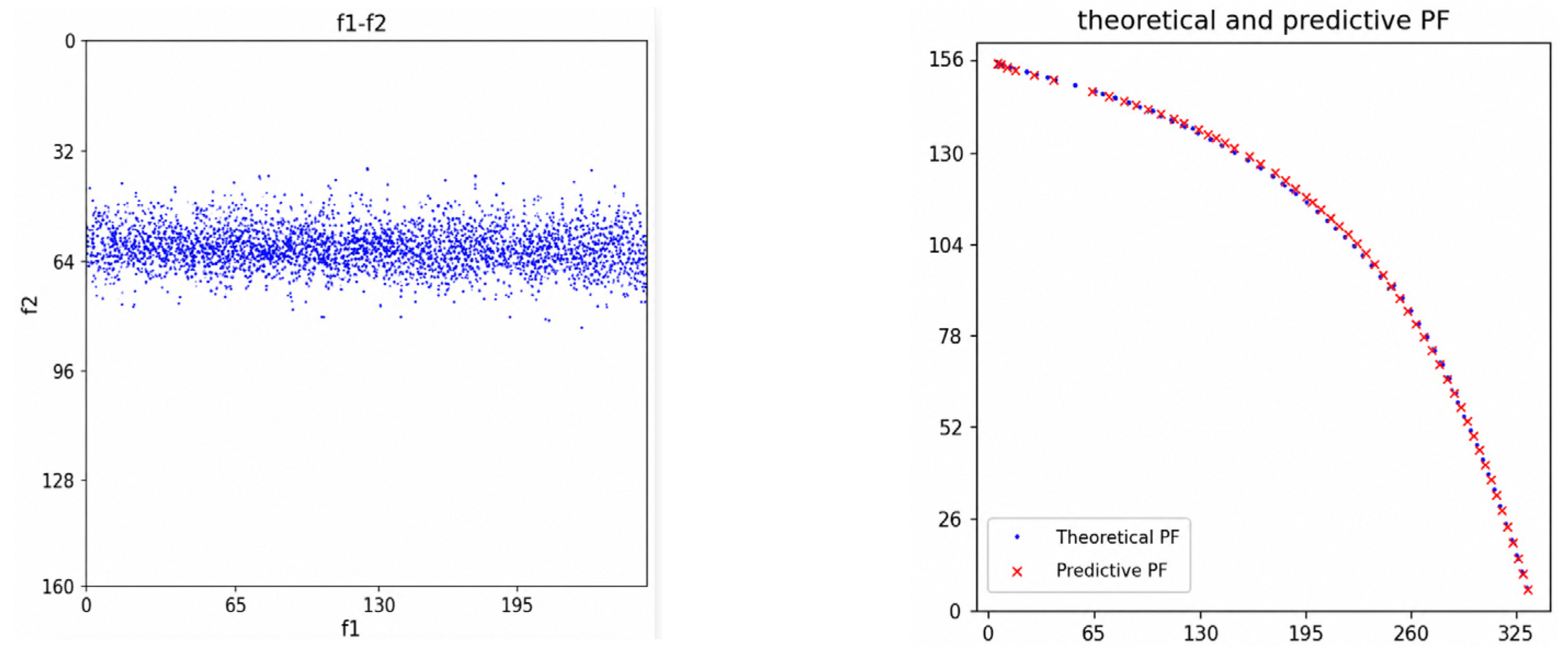
The supervised CNN output is evaluated against theoretical or high-density sampled reference fronts. Figure 1 shows SCH. The predicted boundary follows the convex reference geometry, while the archived proximity statistic Υ = 0.076343 indicates that visible shape agreement should not be interpreted as exact pointwise recovery.

For FON, POL, KUR, ZDT1, ZDT2, and ZDT4, the archived numerical behavior is summarized in

Table 12. Archived mean and variance of the proximity indicator Υ for the supervised CNN.

Algorithm/Statistic	SCH	FON	POL	KUR	ZDT1	ZDT2	ZDT3	ZDT4	ZDT6
CNN mean	0.076343	0.005515	0.001653	0.015615	0.005941	0.003648	0.007598	0.022549	0.013602
CNN variance	0.080410	1.2672 × 10−5	1.0984 × 10−5	3.5176 × 10−5	1.4636 × 10−5	2.7381 × 10−5	9.3166 × 10−5	0.000146	7.8388 × 10−5

and

Table 13. Archived distribution indicator Δ for the supervised CNN.

Algorithm	SCH	FON	POL	KUR	ZDT1	ZDT2	ZDT3	ZDT4	ZDT6
CNN	1.3542	0.2694	0.9637	0.5198	0.3572	0.4201	N/A	0.4688	0.4610

rather than repeated through additional figures. The proximity and spacing patterns remain problem-dependent because the supervised objective emphasizes occupancy reconstruction and boundary localization rather than an explicit crowding-distance or hypervolume term.

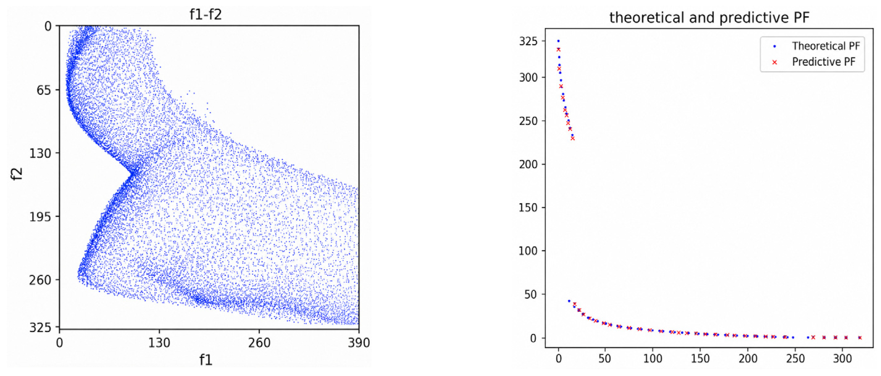
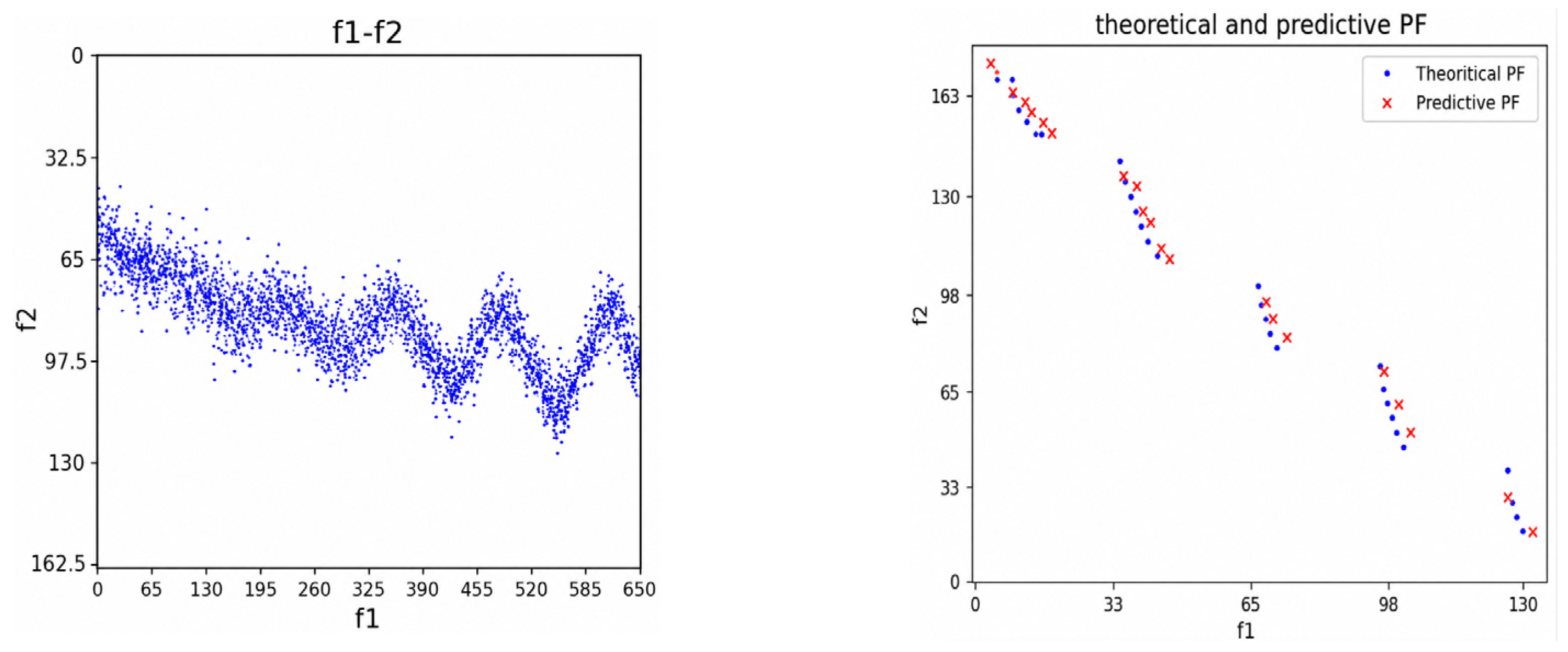
Figure 2 retains ZDT3 because its reference front is disconnected. The CNN recovers the separated segments with Υ = 0.007598. The endpoint-based Δ statistic is not interpreted for this problem because one global pair of endpoints does not represent spacing across five disconnected components.

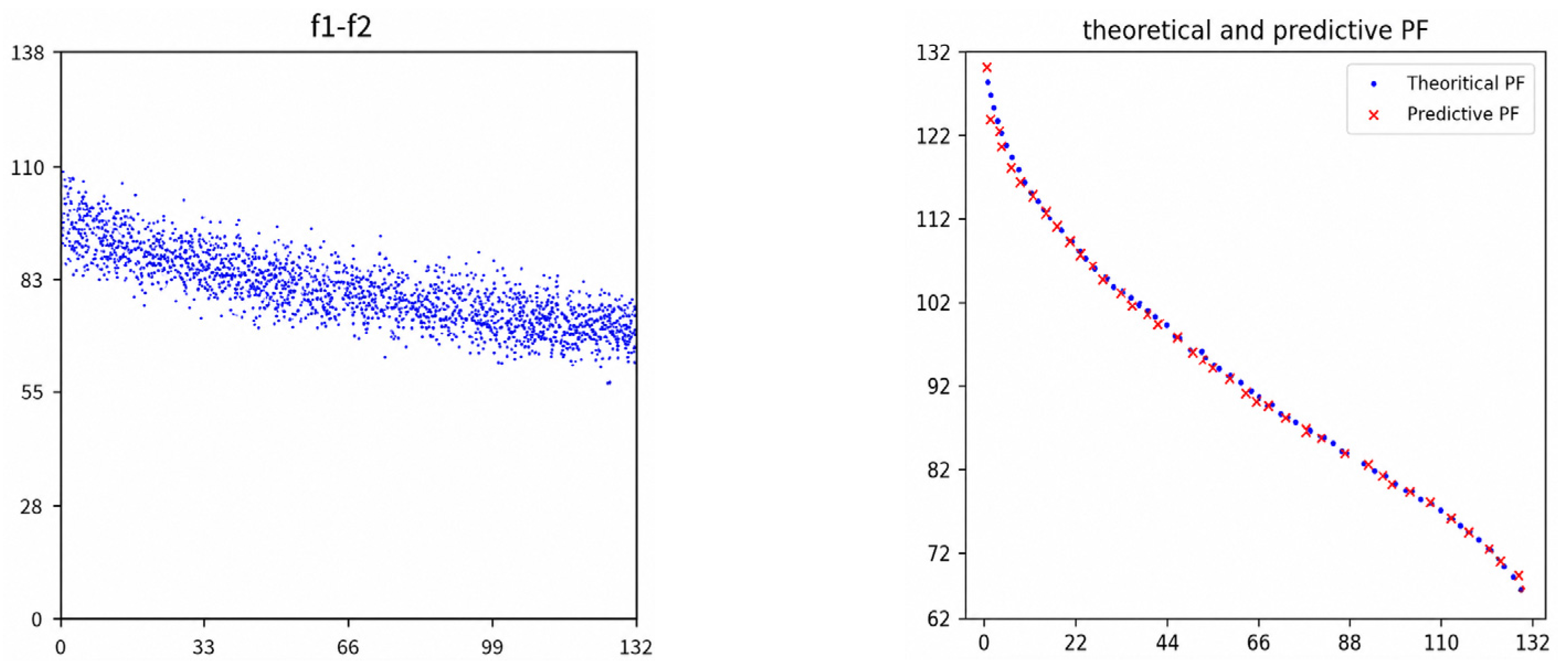
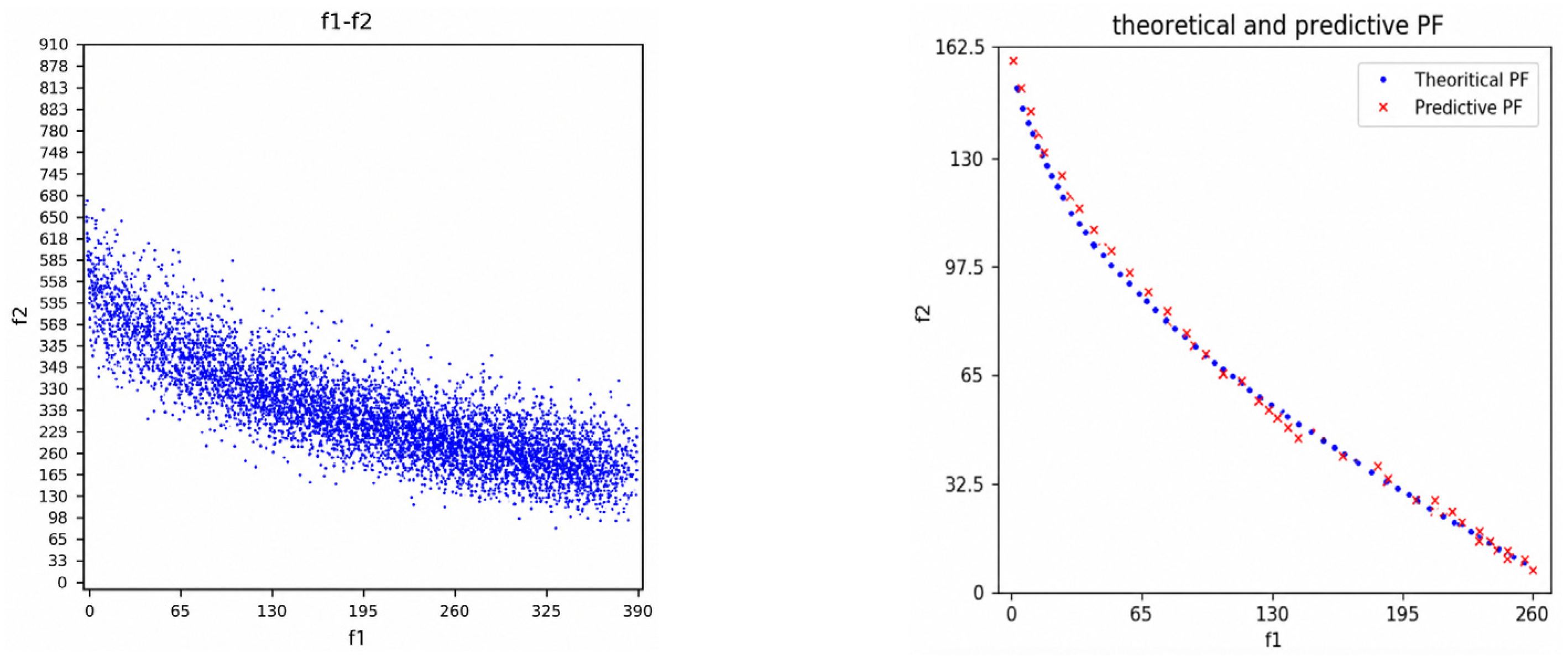
Figure 3 retains ZDT6 because its front is nonlinear and unevenly distributed. The CNN preserves the principal reference shape with Υ = 0.013602, while the archived Δ = 0.4610 describes spacing within the sampled prediction rather than establishing superiority over another optimizer.

Table 12 shows that the archived proximity behavior varies across benchmark geometries. Lower Υ values on POL, ZDT1, ZDT2, ZDT3, and ZDT6 indicate closer sampled boundaries, whereas the larger SCH value shows that visual shape agreement does not guarantee uniform pointwise accuracy. The table is interpreted as a descriptive characterization of the CNN module.

Table 13 shows that the spacing behavior is problem-dependent because no explicit crowding-distance or hypervolume term is used during CNN training. The ZDT3 entry is not interpreted because the endpoint-based definition is unsuitable for disconnected fronts. If spacing control is required, a distribution-aware training term or post-processing stage should be introduced and validated separately.

5.2. Feature Visualization and Deterministic Pareto-Front Extraction

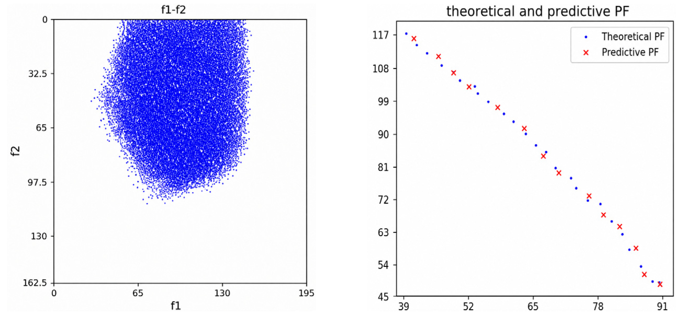
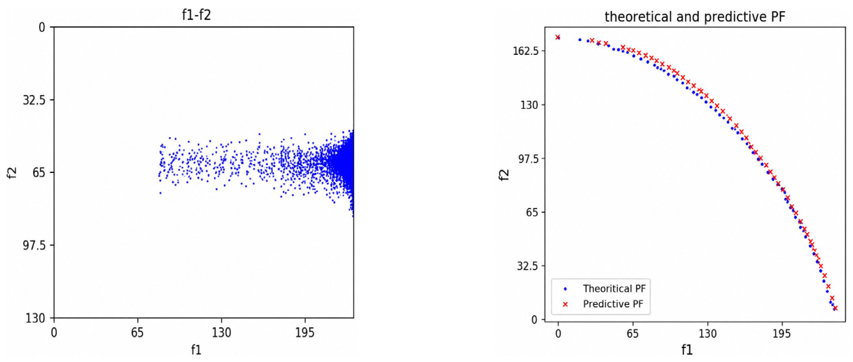
Intermediate-layer visualization is used to inspect whether the CNNs respond to local objective-space structures. Figure 4 shows that Network I preserves occupancy traces and boundary information on ZDT3, which is consistent with its reconstruction role, but does not by itself establish exact non-dominance.

Figure 5 shows a representative feature response of Network II. The activation is concentrated near boundary structures rather than over the complete occupied region, which is consistent with sampled boundary approximation.

The fixed extractor was first applied to a 127 × 127 occupancy image, equivalent to 16,129 occupied cells when the grid is full. Figure 2 makes the extracted boundary directly visible. Under the stated environment and u = 15, the archived average extraction time is 0.047 s, as shown in Figure 6.

Figure 7 shows the 1024 × 1024 case, equivalent to 1,048,576 occupied cells when the grid is full. Because the boundary occupies a small portion of the image, correctness is established by the direct verification procedure in Section 4.4 rather than by visual inspection alone. The archived average extraction time is 2.726 s.

Figure 8 shows the 2048 × 2048 case, equivalent to 4,194,304 occupied cells when the grid is full. The archived average extraction time is 19.956 s. This result documents the runtime trend of the fixed grid operation on the reported hardware; it is not used to infer superiority over specialized two-objective sorting.

5.3. Exploratory Reinforcement-Learning Feasibility on SCH

The SCH reinforcement-learning study is reported as an exploratory feasibility analysis of state, action, and dominance-reward definitions. The benchmark has one decision variable and a known convex front, so the evidence is limited to whether each formulation can generate a recoverable candidate set.

MOP-DQN produces candidates that follow the expected simple-front trend, but one-state-at-a-time updating and a sparse binary reward restrict the interpretation to proof-of-concept candidate generation.

MOP-AC produces a denser archived candidate set in the reported SCH case. This observation is confined to that case and is not presented as a general stability or performance ranking.

MOP-AC-sample broadens exploration by drawing several candidates from each distribution state. The accumulated occupancy image is then processed by the fixed extractor and cell archive. This branch demonstrates a concrete module connection, while broader nonlinear, disconnected, multimodal, constrained, and higher-dimensional cases remain outside the present evidence.

5.4. Methodological Interpretation and Contribution Boundary

The architecture is modular rather than a mandatory serial solver. The supervised route maps sparse sampled objective vectors to a reconstructed occupancy image and then to a sampled boundary approximation. The rule-based route accepts candidate vectors from any sampler, evolutionary procedure, or reinforcement-learning agent and applies the fixed extractor directly. MOP-DQN and MOP-AC maintain non-dominated sets internally and do not require a CNN connection, whereas MOP-AC-sample accumulates an occupancy image and invokes the fixed extractor at termination. During rasterization, each objective vector y = f(x) is assigned to a cell (i, j). The occupancy bit is set to one, while the tuple containing the sample index, x, and y is appended to the corresponding cell archive A_ij. The CNN branches read only the occupancy image. The deterministic branch uses the occupancy map for fixed cross-correlation and then retrieves A_ij from retained cells for exact vector-level dominance refinement. Table 9 summarizes the complete data flow, archive construction, and admissible invocation relationships.

5.5. Limitations and Engineering Implications

Quantization error is controlled by the cell widths h₁ and h₂. If a cell center represents all vectors assigned to that cell, Equation (A2) gives the coordinate-wise and Euclidean positional bounds. Lower resolution increases this bound and collision probability, whereas higher resolution increases grid memory and convolution work. Table 12 reports the archived mean and variance of Υ for the supervised CNN. Because the available evidence is aggregate, the discussion is descriptive and does not use confidence intervals, significance tests, hypervolume, IGD, or GD+ to support inferential claims.

The reinforcement-learning evidence remains confined to SCH. Accordingly, Section 5.3 reports only feasibility observations, while broader MORL and Actor-Critic comparisons are specified as subsequent validation rather than inferred from the present case.

The computational boundary is made explicit by C_total = N_evalC_f + C_raster + C_extract in Equation (A5), where C_f is the cost of one objective evaluation. The reported extractor timings begin after objective values are available. If C_f is large, as in simulation-based engineering design, N_evalC_f will dominate and the grid extractor cannot remove that bottleneck; a surrogate, Bayesian strategy, or adaptive sampling method would still be required. The extractor is most applicable to inexpensive objectives, previously generated candidate archives, repeated post-processing, or workflows in which many candidate vectors must be filtered on parallel hardware.

6. Conclusions

6.1. Main Conclusions

This study develops a benchmark-based method for strictly two-objective objective-space approximation and non-dominated extraction. Sampled vectors are represented as occupancy images, the supervised CNNs approximate occupancy and boundary patterns, and the fixed extractor applies an explainable dominance rule followed by cell-archive refinement. The methodological motivation includes future option-pricing model selection and calibration in financial mathematics and quantitative economic analysis, but the present conclusions concern SCH, FON, POL, KUR, and ZDT synthetic benchmarks.

The principal algorithmic contribution is the deterministic cross-correlation construction rather than the elementary central inversion on which its quadrant interpretation is based. Under the declared coordinate convention, repeated passes cover the relevant dominance region at the cell level. Exact vector-level reporting additionally requires the cell archive because binary occupancy alone cannot resolve raster collisions. The reported 127 × 127 to 2048 × 2048 cases document feasibility and regular parallel structure, not a universal asymptotic or empirical advantage over specialized sorting.

MOP-DQN, MOP-AC, and MOP-AC-sample are secondary exploratory modules. Their SCH results illustrate alternative state representations and dominance-based rewards, while broader benchmark, baseline, ablation, and repeated-run validation are required before general reinforcement-learning conclusions can be drawn.

6.2. Research Directions

Future research should document complete training controls, conduct independent repetitions, report HV, IGD, and GD+ where appropriate, measure peak memory, and compare the fixed extractor with specialized two-objective sorting on identical hardware. The reinforcement-learning branch should be evaluated against fully specified MORL and modern actor-critic baselines on nonlinear, disconnected, multimodal, constrained, and higher-dimensional problems. The next application step is to replace the synthetic objective mapping with a market-calibrated option-pricing formulation in which parametric pricing coefficients and a nonparametric residual module are optimized under paired objectives such as pricing error and hedging stability.

References

1. Miettinen, K. Nonlinear Multiobjective Optimization; Kluwer Academic Publishers: Boston, MA, USA, 1999. [Google Scholar]
2. Ehrgott, M. Multicriteria Optimization, 2nd ed.; Springer: Berlin/Heidelberg, Germany, 2005. [Google Scholar]
3. Deb, K.; Pratap, A.; Agarwal, S.; Meyarivan, T. A fast and elitist multiobjective genetic algorithm: NSGA-II. IEEE Trans. Evol. Comput. 2002, 6, 182–197. [Google Scholar] [CrossRef] [Scilit]
4. Zitzler, E.; Laumanns, M.; Thiele, L. SPEA2: Improving the Strength Pareto Evolutionary Algorithm; TIK-Report 103; ETH Zurich: Zurich, Switzerland, 2001. [Google Scholar]
5. Emmerich, M.T.M.; Deutz, A.H. A tutorial on multiobjective optimization: Fundamentals and evolutionary methods. Nat. Comput. 2018, 17, 585–609. [Google Scholar] [CrossRef] [Scilit] [PubMed]
6. Blank, J.; Deb, K. Pymoo: Multi-objective optimization in Python. IEEE Access 2020, 8, 89497–89509. [Google Scholar] [CrossRef] [Scilit]
7. Lavinas, Y.; Ladeira, M.; Ochoa, G.; Aranha, C. Component-wise analysis of automatically designed multiobjective algorithms on constrained problems. In Proceedings of the Genetic and Evolutionary Computation Conference Companion, Boston, MA, USA, 9–13 July 2022. [Google Scholar]
8. Nebro, A.J.; Durillo, J.J.; Luna, F.; Alba, E. On the automatic design of multi-objective particle swarm optimizers. Swarm Intell. 2024, 18, 105–139. [Google Scholar] [CrossRef] [Scilit]
9. Hanne, T.; Dornberger, R. A review of the evolution of multi-objective evolutionary algorithms. Comput. Mater. Contin. 2025, 85, 4203–4236. [Google Scholar] [CrossRef] [Scilit]
10. Daulton, S.; Balandat, M.; Bakshy, E. Parallel Bayesian optimization of multiple noisy objectives with expected hypervolume improvement. Adv. Neural Inf. Process. Syst. 2021, 34, 2187–2200. [Google Scholar]
11. Li, H.; Gao, P.; Tan, H.; Li, H.; Zhu, H.; Jiang, M.; Ni, Y.; He, Y.; Huang, J.; Zhu, Y.; et al. Interaction-aware dexterous robot for minimally invasive transcanal inner ear interventions. Nat. Commun. 2026, 17, 5658. [Google Scholar] [CrossRef] [Scilit] [PubMed]
12. Lai, C.-H.; Wu, T.-E.; Wang, C.-C. Enhancing Information Security in Smart Manufacturing Through Least Significant Bit Steganography in Engineering Drawings. J. Comput. Inf. Sci. Eng. 2025, 25, 091006. [Google Scholar] [CrossRef] [Scilit]
13. Fan, M.; Su, D.; Zhang, N.; Cai, G.-J.; Chen, X.-S. Coupled effects of particle multilevel morphology and intermediate principal stress ratio on the macro-and micro-mechanical behavior of granular soils: A DEM study. Transp. Geotech. 2026, 62, 102142. [Google Scholar] [CrossRef] [Scilit]
14. Yao, S.; Li, Z.; Guan, R.; Xia, M.; Hu, F.; Cao, K.; Xu, S.; Zhu, X.; Liu, R.W.; Ding, W. GIF-Calib: Geometry-Intensity Fusion for 4D Radar-Camera Calibration in Autonomous Driving Vehicles. Inf. Fusion 2026, 136, 104510. [Google Scholar] [CrossRef] [Scilit]
15. Choi, H.S.; Cheng, T. Spatial cognition and emotion simulation in urban interior environments using agent-based modelling. Int. J. Urban Sci. 2026, 30, 1–24. [Google Scholar] [CrossRef] [Scilit]
16. Shen, M.; Sun, J.; Suo, P.; Zhang, X.; Yuan, Z.; Wang, Y.; Li, C.; Xu, L. Interface-Sensitive Electrical Capacitance-Ratio Tomography for Supercavity Profile Reconstruction in Open-domain. IEEE Trans. Instrum. Meas. 2026, 75, 4502010. [Google Scholar] [CrossRef] [Scilit]
17. Yin, Y.; Liang, Y.; Zhang, X.; Qin, Z.; Han, X. A reduced-order Galerkin-projected flame transfer model for coupled dual jet diffusion flames based on mixture fraction. Combust. Flame 2026, 291, 115157. [Google Scholar] [CrossRef] [Scilit]
18. Sun, T.; Zhang, J.; Yang, H.; Yang, J.; Cheng, L. Bidirectional Mamba-Based Continuous Prediction of Human Motion Intention Using Multisource Information Fusion. IEEE Trans. Autom. Sci. Eng. 2025, 23, 212–221. [Google Scholar] [CrossRef] [Scilit]
19. Gao, M.; Zhou, S.; Gu, W.; Fan, J.; Guan, A.; Zhu, H.; Wei, L.; Hu, Z. Enhancing distribution system state estimation under limited measurements: Leveraging large language model and multimodal information. CSEE J. Power Energy Syst. 2026, 12, 622–631. [Google Scholar] [CrossRef] [Scilit]
20. Bao, Y.; Wang, X.; Hu, H.; Zuo, Y.; Tu, S.; Zhang, P.; Qi, Q.; Deng, H. Transient vibration response analysis of underwater cylindrical shells based on precise integration method. Ocean Eng. 2026, 358, 125881. [Google Scholar] [CrossRef] [Scilit]
21. Xu, B.; Lu, Q.; Gao, X.; Li, B.; Li, W.; He, J.; Gong, D.; Fan, Z. An Optimized Collaborative Routing Model for Trucks and Heterogeneous Drones in Delivery and Pickup Services. IEEE Trans. Intell. Transp. Syst. 2026, 27, 9113–9130. [Google Scholar] [CrossRef] [Scilit]
22. Hu, P.; Zhang, R.; Chen, L.; Li, L.; Tang, Q.; Hewitt, A.J. Atomization Index to Bridge the Physicochemical Properties of Polymer-Surfactant Adjuvants and Multivariate Spray Metrics: Guiding Pesticide Formulation Efficient Design. Engineering 2026. [Google Scholar] [CrossRef] [Scilit]
23. He, Y.; Liu, X.; Yang, R.; Chen, Q.; Deng, B.; Jin, M.; Wang, F. Deblur of infrared thermal images of in-service wind turbine blade based on rotational motion flow. Measurement 2026, 287, 122462. [Google Scholar] [CrossRef] [Scilit]
24. Wang, L.; Zhang, B.; Li, Y.; Liu, B.; Tong, C.; Xiong, H.; Chen, G.; Hong, Z.; Zhang, C.; Tian, Y. Uplift resistance mechanism of pipes in lightweight backfill material of ceramsite. Comput. Geotech. 2026, 192, 107927. [Google Scholar] [CrossRef] [Scilit]
25. Zhang, T.; Wang, L.; Chen, L.; Lu, W.; Hao, D.; Shao, W.; Zhang, C.; Tian, Y. Numerical analysis of post-cyclic ultimate bearing capacity of helical anchors in clay. Ocean Eng. 2026, 352, 124583. [Google Scholar] [CrossRef] [Scilit]
26. Kang, M.; Liang, Y.; Zhao, B.; Liu, J.; Wang, X.; Wu, C.; Li, Q.; Zhang, J.; Tian, W. Machine learning-based detection technology for electron beam and laser processing. Opt. Laser Technol. 2026, 201, 115292. [Google Scholar] [CrossRef] [Scilit]
27. Zhang, P.; Hou, D.; Li, M.; Zhou, Q.; Guo, G.; Sun, F.; Liu, K. Highly-reliable underwater synchronization based on optical two-way time transfer at sub-nanosecond-level. Opt. Laser Technol. 2026, 203, 115624. [Google Scholar] [CrossRef] [Scilit]
28. Liu, W.; Zhu, L.; Huo, X.-J.; Ma, X.-W.; Li, J.-H.; Cheng, X.-X. Shape-finding for a triple-tower spatial double-cable suspension bridge with upper hangers. Eng. Struct. 2026, 366, 123403. [Google Scholar] [CrossRef] [Scilit]
29. Jiang, L.; Fang, H.; Shang, X.; Zhang, Z. Hierarchical Clustering Weighted Gaussian Process Regression Low-Fidelity Model and Application in Airfoil Drag Coefficients Prediction. IEEE Trans. Aerosp. Electron. Syst. 2026, 62, 9070–9081. [Google Scholar] [CrossRef] [Scilit]
30. Luo, H.; Feng, Q.; Sun, W.; Li, W.; Li, Q.; Zhao, W.; Liu, Z. FD-Mamba With Neural Observer and Frequency-Enhanced Update for Incipient Feeder Fault Detection. IEEE Internet Things J. 2026, 13, 20761–20772. [Google Scholar] [CrossRef] [Scilit]
31. Yang, C.; Yang, S.; He, Y.; Fan, L.; Gao, X.; Tang, M.; Sun, J. Research on Defect Detection Performance of Silicon Carbide Wafer Surface Based on ESN-YOLOv8 Algorithm. Comput. Mater. Sci. 2026, 268, 114656. [Google Scholar] [CrossRef] [Scilit]
32. Fan, L.; He, Y.; Mo, Y.; Cao, Y. An Interpretable Ensemble Machine Learning Model for Predicting Carbon Dioxide Adsorption on Magnesium Oxide-Based Sorbents. Environ. Res. 2026, 297, 124126. [Google Scholar] [CrossRef] [Scilit] [PubMed]
33. Chen, L. Beyond External Constraints: The Missing Dimension of AI Governance. SSRN 2026, 6449738. [Google Scholar] [CrossRef] [Scilit]
34. Li, Q.; Luo, H.; Cheng, H.; Deng, Y.; Sun, W.; Li, W.; Liu, Z. Incipient Fault Detection in Power Distribution System: A Time–Frequency Embedded Deep-Learning-Based Approach. IEEE Trans. Instrum. Meas. 2023, 72, 2507914. [Google Scholar] [CrossRef] [Scilit]
35. Chen, D.; Xu, C.; Yu, J.; Wang, Q.; Fang, H.; Yin, S.; Lookman, T.; Chen, R. Interpretable Machine Learning Framework for Nb–Si-Based Alloy Design with Enhanced Fracture Toughness. Adv. Sci. 2026, 13, e75815. [Google Scholar] [CrossRef] [Scilit] [PubMed]
36. Wu, X.; Zou, B.; Lu, C.; Wang, L.; Zhang, Y.; Wang, H. Dynamic Security Computing Framework With Zero Trust Based on Privacy Domain Prevention and Control Theory. IEEE J. Sel. Areas Commun. 2025, 43, 2266–2278. [Google Scholar] [CrossRef] [Scilit]
37. Chen, J.; Shao, Z.; Zhu, H.; Chen, Y.; Li, Y.; Zeng, Z.; Yang, Y.; Wu, J.; Hu, B. Sustainable Interior Design: A New Approach to Intelligent Design and Automated Manufacturing Based on Grasshopper. Comput. Ind. Eng. 2023, 183, 109509. [Google Scholar] [CrossRef] [Scilit]
38. Luo, H.; Li, Q.; Zhou, H.; Sun, W.; Li, W.; Liu, Z.; Ji, Y.; Ding, L. Weak Single Phase-to-Ground Fault Time Detection With Learnable-Parameter-Driven DSP-Enhanced Transformer. IEEE Trans. Smart Grid 2026, 17, 1693–1708. [Google Scholar] [CrossRef] [Scilit]
39. Chen, J.; Yin, H.; Zhang, K.; Ren, Y.; Zeng, H. Integration of Neural Networks in Brain–Computer Interface Applications: Research Frontiers and Trend Analysis Based on Python. Eng. Appl. Artif. Intell. 2025, 151, 110654. [Google Scholar] [CrossRef] [Scilit]
40. Wu, X.; Dong, J.; Bao, W.; Zou, B.; Wang, L.; Wang, H. Augmented Intelligence of Things for Emergency Vehicle Secure Trajectory Prediction and Task Offloading. IEEE Internet Things J. 2024, 11, 36030–36043. [Google Scholar] [CrossRef] [Scilit]
41. Xu, C.; Chen, D.; Zhang, X.; Wang, Q.; Yu, J.; Wang, S.; Guo, J.; Fu, H.; Chen, R.; Lookman, T. High Temperature Nb-Si Alloys Using Data Science: Optimization of Fracture Toughness and High-Temperature Strength. Nat. Commun. 2026. [Google Scholar] [CrossRef] [Scilit] [PubMed]
42. Wu, X.; Wang, H.; Zhang, Y.; Zou, B.; Hong, H. A Tutorial-Generating Method for Autonomous Online Learning. IEEE Trans. Learn. Technol. 2024, 17, 1558–1567. [Google Scholar] [CrossRef] [Scilit]
43. Mnih, V.; Kavukcuoglu, K.; Silver, D.; Rusu, A.A.; Veness, J.; Bellemare, M.G.; Graves, A.; Riedmiller, M.; Fidjeland, A.K.; Ostrovski, G.; et al. Human-level control through deep reinforcement learning. Nature 2015, 518, 529–533. [Google Scholar] [CrossRef] [Scilit] [PubMed]
44. Schulman, J.; Wolski, F.; Dhariwal, P.; Radford, A.; Klimov, O. Proximal policy optimization algorithms. arXiv 2017, arXiv:1707.06347. [Google Scholar]
45. Hayes, C.F.; Radulescu, R.; Bargiacchi, E.; Kallstrom, J.; Macfarlane, M.; Reymond, M.; Verstraeten, T.; Zintgraf, L.M.; Dazeley, R.; Heintz, F.; et al. A practical guide to multi-objective reinforcement learning and planning. Auton. Agents Multi-Agent Syst. 2022, 36, 26. [Google Scholar] [CrossRef] [Scilit]
46. Alegre, L.N.; Felten, F.; Talbi, E.G.; Danoy, G.; Nowe, A.; Bazzan, A.L.C.; da Silva, B.C. MO-Gym: A library of multi-objective reinforcement learning environments. In Proceedings of the 34th Benelux Conference on Artificial Intelligence and Machine Learning, Mechelen, Belgium, 7–9 November 2022. [Google Scholar]
47. Felten, F.; Alegre, L.N.; Nowe, A.; Bazzan, A.L.C.; Talbi, E.G.; Danoy, G.; da Silva, B.C. A toolkit for reliable benchmarking and research in multi-objective reinforcement learning. Adv. Neural Inf. Process. Syst. 2023, 36, 23671–23700. [Google Scholar] [CrossRef] [Scilit]
48. Felten, F.; Talbi, E.G.; Danoy, G. Multi-objective reinforcement learning based on decomposition: A taxonomy and framework. J. Artif. Intell. Res. 2024, 79, 679–723. [Google Scholar] [CrossRef] [Scilit]
49. Seurin, P.; Shirvan, K. Multi-objective reinforcement learning-based approach for pressurized water reactor optimization. arXiv 2023, arXiv:2312.10194. [Google Scholar]
50. Zhang, C.; Wu, F.; Huang, M.; Ma, J.; Ma, H.; Liu, Y. Generative AI for planar substrate integrated waveguide microwave filters: Autonomous circuit synthesis with coupling-controlled topology generation. IEEE Trans. Microw. Theory Tech. 2026, 74, 1740–1755. [Google Scholar] [CrossRef] [Scilit]
51. Guo, Z.; Sha, X.; Sang, X.; Zhang, J.; Wang, S.; Zhao, Y. CTPEM: A cross-temporal progressive enhancement model tackling object-level building damage detection and vanishing small features. IEEE Trans. Geosci. Remote Sens. 2025, 63, 5643012. [Google Scholar] [CrossRef] [Scilit]
52. Yuan, J.; Zhou, L.; He, M.; Luo, C.; Zhang, J. A lightweight dual path Kolmogorov-Arnold convolution network for medical optical image segmentation. Neurocomputing 2026, 659, 131776. [Google Scholar] [CrossRef] [Scilit]
53. Wang, Z.; Zhang, X.; Li, W.; Feng, Z. Real-time UUV obstacle avoidance through flexible steering technology based on improved Soft Actor-Critic framework. IEEE Trans. Instrum. Meas. 2025, 74, 3003514. [Google Scholar] [CrossRef] [Scilit]
54. Harrison, K.R.; Asilian Bidgoli, A.; Rahnamayan, S.; Deb, K. Image-based benchmarking and visualization for large-scale global optimization. Appl. Intell. 2022, 52, 4161–4191. [Google Scholar] [CrossRef] [Scilit]
55. Singh, G.; Gupta, S.; Lease, M.; Dawson, C. A hybrid two-stage neural optimization for Pareto-front extraction. arXiv 2021, arXiv:2101.11684. [Google Scholar]
Figure 1. SCH objective-space reconstruction and sampled Pareto-front approximation. Left: rasterized occupancy in the f1–f2 objective plane. Right: theoretical reference front (blue points) and CNN-predicted front (red crosses); both axes represent dimensionless benchmark objective values.
Symmetry 18 01344 g001
Figure 2. ZDT3 objective-space reconstruction and sampled disconnected Pareto-front approximation. Left: rasterized occupancy in the f1–f2 objective plane. Right: theoretical reference segments (blue points) and CNN prediction (red crosses); objective values are dimensionless.
Symmetry 18 01344 g002
Figure 3. ZDT6 objective-space reconstruction and sampled Pareto-front approximation. Left: rasterized occupancy in the f1–f2 objective plane. Right: theoretical reference front (blue points) and CNN prediction (red crosses); objective values are dimensionless.
Symmetry 18 01344 g003
Figure 4. Intermediate-layer visualization of Network I on ZDT3. Left: representative reconstructed occupancy response in raster coordinates. Right: the corresponding theoretical reference front and CNN-predicted front in dimensionless objective-value coordinates.
Symmetry 18 01344 g004
Figure 5. Representative feature response of Network II. Left: intermediate boundary-sensitive activation in raster coordinates. Right: theoretical reference front and CNN-predicted boundary in dimensionless objective-value coordinates.
Symmetry 18 01344 g005
Figure 6. Fixed-kernel extraction on a 127 × 127 occupancy image. Left: sampled objective-space occupancy; right: theoretical reference cells and extracted boundary cells. The axes are raster coordinates and therefore have no physical unit.
Symmetry 18 01344 g006
Figure 7. Fixed-kernel extraction on a 1024 × 1024 occupancy image. Left: sampled objective-space distribution; right: comparison between the theoretical Pareto front and the predicted Pareto front. The axes represent the original objective values.
Symmetry 18 01344 g007
Figure 8. Fixed-kernel extraction on a 2048 × 2048 occupancy image. Left: sampled objective-space occupancy; right: theoretical Pareto front and predictive Pareto front. The axes represent the original objective values.
Symmetry 18 01344 g008