Communication-Efficient Affine Formation Maneuver Control for Unmanned Surface Vehicles via Hybrid Event-Driven Interaction

Abstract

With the rapid development of Internet of Things (IoT) technology, the formation control of unmanned surface vehicles (USVs) has attracted increasing attention in marine applications. However, in practical marine missions, the implementation of affine formation maneuver control (AFMC) still faces challenges caused by limited communication resources and restricted interaction frequency of onboard communication devices. To address these issues, this paper proposes a hybrid event-driven interaction mechanism (HEIM) for AFMC of USVs. In this mechanism, a clock variable is first introduced to regulate the interaction process, such that excessively frequent information exchanges can be avoided and the interaction interval can satisfy the minimum communication interval (MCI) required by onboard hardware. However, when the clock variable reaches its lower bound, an interaction may be compulsorily triggered, which introduces a maximum interaction interval constraint. To remove this restriction, an additional threshold is further incorporated as a secondary interaction judgment condition. In this way, the proposed mechanism not only preserves an adjustable MCI but also avoids unnecessary interactions caused solely by the clock variable, thereby further improving communication efficiency. Theoretical analysis and simulation results demonstrate the effectiveness of the proposed method.

1. Introduction

Driven by the rapid advancement of Internet of Things (IoT) technology, the cooperative operation of multiple unmanned surface vehicles (USVs) has become an important research topic due to its broad applications in maritime missions, including environmental monitoring, emergency search and rescue, and ocean resource development [1,2,3,4,5]. Due to the inherent limitations of a single USV in terms of sensing range, endurance, and task execution capability, coordinated multi-USV operation has emerged as a prevalent paradigm for extensive maritime missions [6,7,8]. To support such missions, cooperative formation control has emerged as one of the core technologies in this field [9,10]. In recent years, considerable efforts have been devoted to the formation control of multi-agent systems [11,12]. These studies have led to a variety of representative approaches, including relative-position-based [13], distance-based [14], bearing-based [15], similarity-based [16], and affine-formation-based methods [17]. Among these approaches, affine formation maneuver control (AFMC) has emerged as a promising framework because of its capability to realize flexible formation transformations [18]. AFMC can generate rich maneuvering behaviors, including translation, rotation, scaling, and shearing. This feature makes it particularly suitable for formation reconfiguration in complex marine environments and further broadens the operational scope of coordinated multi-vehicle systems [19,20,21]. To realize AFMC, USV nodes need to exchange information in real time to ensure the reliable execution of formation tasks [22]. Given the limited onboard space and payload capacity of USVs, their available energy during missions is usually constrained. Therefore, high-frequency information exchange may shorten operational endurance. Meanwhile, onboard communication devices have finite interaction capability. Once the interaction interval is shorter than the hardware-allowable MCI, communication congestion and data accumulation may occur, leading to degraded interaction reliability.

In response to the issue of limited onboard energy, event-driven mechanisms (EIMs) have garnered increasing attention in recent years. Among them, static and dynamic EIMs are widely studied [23,24,25,26,27,28]. The static EIM activates information exchange when the measurement error exceeds a predefined threshold, thereby suppressing redundant interactions [23]. Compared with this fixed-threshold design, the dynamic EIM introduces an auxiliary dynamic variable into the interaction condition, which enhances the adaptability of the interaction mechanism [28]. This design can further reduce communication consumption and extend the operational endurance of USVs in long-duration missions. Although static and dynamic EIMs can theoretically preclude Zeno behavior, they generally cannot provide an explicit MCI. The guaranteed inter-event interval is only positive and may approach zero when the measurement error becomes large. Therefore, Zeno behavior is avoided in a mathematical sense, but frequent interactions may still be triggered in practical implementations. This may cause the communication frequency to exceed the hardware capability of onboard devices, leading to data accumulation and communication congestion. To overcome this limitation, MCI-based EIMs have been developed in [29,30,31]. By introducing a resettable variable into the interaction condition, these methods ensure that the decay time from the reset value to the triggering boundary has a positive lower bound, thereby explicitly guaranteeing a computable MCI. Benefiting from this advantage, such MCI-based designs have been extended to AFMC of USVs to reduce interaction frequency while guaranteeing an explicit MCI [32]. Nevertheless, two limitations remain in existing MCI-based methods. On the one hand, the guaranteed MCIs are usually not actively tunable, but are passively determined by system-related parameters, such as adaptive variables and stress-matrix-dependent terms. Consequently, the interaction interval cannot be readily adjusted to accommodate different onboard communication capabilities. Moreover, the use of a clock variable may impose a maximum interaction interval (MII). Specifically, the clock variable enforces an interaction once it reaches the prescribed threshold. Moreover, since its decreasing rate is lower bounded by a positive constant, the time required to reach this threshold is upper bounded. As a result, a maximum interaction interval (MII) constraint is introduced, which may cause forced information exchange and unnecessary energy consumption. These issues motivate the development of a more flexible interaction strategy that can actively adjust the MCI while eliminating the MII constraint.

Based on the above analysis, this paper proposes a hybrid event-driven interaction mechanism (HEIM) for affine formation maneuver control of USVs. The core advantages of the proposed mechanism are mainly reflected in the following two aspects:

(1)

A HEIM is developed to systematically regulate information interactions. By introducing clock variables, the MCI can be explicitly prescribed through tunable parameters, thereby ensuring compatibility with onboard communication hardware. Unlike existing MCI-based methods with passively determined MCIs [29,30,31,32], the MCI of HEIM is determined only by the designed parameters, thereby providing a flexible and hardware-compatible interaction design.

(2)

To remove the MII constraint caused by the clock variable, an additional threshold is introduced as a secondary interaction condition. With this dual judgment structure, the proposed HEIM not only satisfies the communication capability of practical hardware but also removes the MII constraint inherent in conventional MCI-based mechanisms [29,30,31,32].

Notations. Let ${\mathbb{R}}^n$ and ${\mathbb{R}}^{m\times n}$ denote the n-dimensional Euclidean space and the set of $m\times n$ real matrices, respectively. For a vector, $\parallel ·\parallel$ denotes the Euclidean norm, and for a scalar, $|·|$ denotes its absolute value. $I_n$ represents the n-dimensional identity matrix, and ${\mathbf{1}}_n$ denotes the n-dimensional column vector with all entries equal to one. For a symmetric matrix, ${\lambda }_{\min }(·)$ and ${\lambda }_{\max }(·)$ denote its minimum and maximum eigenvalues, respectively. The symbol ⊗ denotes the Kronecker product.

2. Problem Formulation

2.1. Graph Theory

This paper uses an undirected graph to describe the communication topology among USVs. Let $\mathcal{G}=(\mathcal{V},\mathcal{E})$, where $\mathcal{V}=\{1,2,\dots ,n\}$ denotes the set of vehicles and $\mathcal{E}\subseteq \mathcal{V}\times \mathcal{V}$ denotes the set of bidirectional communication links. If $(j,i)\in \mathcal{E}$, vehicle i can obtain information from vehicle j. In the two-dimensional space ${\mathbb{R}}^d$ with $d=2$, consider a leader–follower formation consisting of n USVs, where $n\ge d+2$. The leader and follower sets are denoted by ${\mathcal{V}}_l$ and ${\mathcal{V}}_f$, with cardinalities $n_l$ and $n_f=n-n_l$, respectively. The position vector of all vehicles is defined as $p={[p_1^T,p_2^T,\dots ,p_n^T]}^T\in {\mathbb{R}}^{dn}$. Correspondingly, the leader and follower position vectors are given by $p_l={[p_1^T,\dots ,p_{n_l}^T]}^T$ and $p_f={[p_{n_l+1}^T,\dots ,p_n^T]}^T$, such that $p={[p_l^T,p_f^T]}^T$. Therefore, the formation is represented by the pair $(\mathcal{G},p)$.

2.2. Affine Formation

Definition 1

(Affine Image). Let $r\in {\mathbb{R}}^{2n}$ denote the nominal configuration of N USVs in ${\mathbb{R}}^2$. Then, the affine image of a nominal configuration refers to the collection of configurations generated from it through affine transformations:

$$\mathsf{\Gamma }\left(r\right)=\{p\in {\mathbb{R}}^{dn}\mid p=(I_n\otimes A)r+1_n\otimes b\}$$

(1)

where $A\in {\mathbb{R}}^{d\times d}$ denotes the affine transformation matrix and $b\in {\mathbb{R}}^d$ represents the translation vector.

Definition 2

(Target Formation). The desired formation $p^{*}\left(t\right)$ is generated by applying a time-varying affine transformation to the nominal configuration, and can be expressed as:

$$p^{*}\left(t\right)=[I_n\otimes A\left(t\right)]r+{\mathbf{1}}_n\otimes b\left(t\right)$$

(2)

where $A\left(t\right)\in {\mathbb{R}}^{d\times d}$ and $b\left(t\right)\in {\mathbb{R}}^d$ are continuously time-varying matrices and vectors used to describe the dynamic affine deformation of the formation during motion.

Lemma 1.

Under the nominal formation framework, the following three propositions are equivalent [33]:

(1) 

The nominal configuration r is affinely localizable by the leaders in ${\mathbb{R}}^d$.

(2) 

One can find a positive semidefinite equilibrium stress matrix Ω such that $\mathrm{rank}\left(\mathsf{\Omega }\right)=n-d-1$ and $\mathrm{Ker}(\mathsf{\Omega }\otimes I_2)=\mathsf{\Gamma }\left(Q\right)$, with its elements defined as follows:

$$[\mathsf{\Omega }{]}_{ij}=\left\{\begin{array}{cc}0,\hfill & i\ne j,(i,j)\notin \mathcal{E}\hfill \\ -{\omega }_{ij},\hfill & i\ne j,(i,j)\in \mathcal{E}\hfill \\ {\displaystyle {\sum }_{j=1}^n}{\omega }_{ij},\hfill & i=j\hfill \end{array}\right.$$

(3)

where ${\omega }_{ij}$ is the stress value corresponding to the edge $(i,j)$. As an equilibrium stress, ${\sum }_{i=1}^n{\omega }_{ij}(p_i-p_j)=0$ holds.

(3) 

For the stress matrix Ω, let $\overline{\mathsf{\Omega }}=\mathsf{\Omega }\otimes I_d$, which can be expressed in block form as:

$$\overline{\mathsf{\Omega }}=\left[\begin{array}{cc}{\mathsf{\Omega }}_{ll}& {\mathsf{\Omega }}_{lf}\\ {\mathsf{\Omega }}_{fl}& {\mathsf{\Omega }}_{ff}\end{array}\right]\otimes I_d=\left[\begin{array}{cc}{\overline{\mathsf{\Omega }}}_{ll}& {\overline{\mathsf{\Omega }}}_{lf}\\ {\overline{\mathsf{\Omega }}}_{fl}& {\overline{\mathsf{\Omega }}}_{ff}\end{array}\right]$$

(4)

where the follower sub-block ${\mathsf{\Omega }}_{ff}\in {\mathbb{R}}^{(n-n_l)\times (n-n_l)}$ is positive definite.

According to the above results, the desired position of the followers satisfies

$$({\mathsf{\Omega }}_{ff}\otimes I_2)p_f^{*}\left(t\right)+({\mathsf{\Omega }}_{fl}\otimes I_2)p_l^{*}\left(t\right)=0.$$

(5)

Since ${\mathsf{\Omega }}_{ff}$ is positive definite, the desired follower position can be obtained as

$$p_f^{*}\left(t\right)=-\left({\mathsf{\Omega }}_{ff}^{-1}{\mathsf{\Omega }}_{fl}\otimes I_2\right)p_l^{*}\left(t\right).$$

(6)

Moreover, as established in [33], the desired heading angles satisfy

$${\psi }_f^{*}\left(t\right)=-{\mathsf{\Omega }}_{ff}^{-1}{\mathsf{\Omega }}_{fl}{\psi }_l^{*}\left(t\right).$$

(7)

Define ${\eta }_i^{*}\left(t\right)=\left[\begin{array}{c}{p}_i^{*}\left(t\right)\\ {\psi }_i^{*}\left(t\right)\end{array}\right],{\eta }_l^{*}\left(t\right)={\mathrm{col}}_{i\in {\mathcal{V}}_l}\left\{{\eta }_i^{*}\left(t\right)\right\},{\eta }_f^{*}\left(t\right)={\mathrm{col}}_{i\in {\mathcal{V}}_f}\left\{{\eta }_i^{*}\left(t\right)\right\}$. Then, the desired position and heading of the followers can be compactly written as

$${\eta }_f^{*}\left(t\right)=-\left({\mathsf{\Omega }}_{ff}^{-1}{\mathsf{\Omega }}_{fl}\otimes I_3\right){\eta }_l^{*}\left(t\right).$$

(8)

2.3. System Model

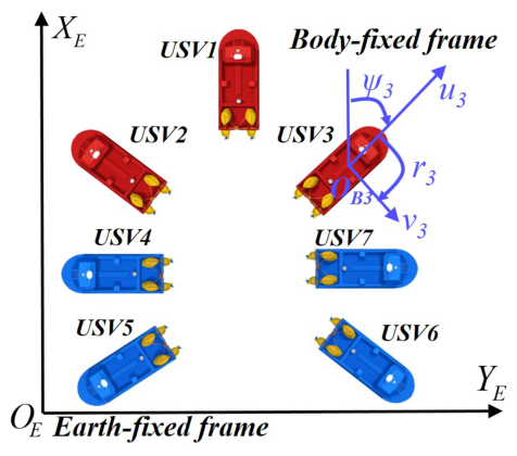
To express the motion of the ith USV, we introduce two distinct reference coordinates, as shown in Figure 1. The USV’s kinematic and dynamic models are given as follows [34]:

$$\left\{\begin{array}{c}{\dot{\eta }}_i=R_i\left({\psi }_i\right){\vartheta }_i\hfill \\ M_i{\dot{\vartheta }}_i+C_i\left({\vartheta }_i\right){\vartheta }_i+D_i\left({\vartheta }_i\right){\vartheta }_i={\tau }_i+d_{wi}\hfill \end{array}\right.$$

(9)

where ${\eta }_i={[x_i,y_i,{\psi }_i]}^T$ denotes the pose of the ith USV in the earth-fixed frame, with $x_i$ and $y_i$ being the position coordinates and ${\psi }_i$ being the yaw angle. The vector ${\vartheta }_i={[u_i,v_i,r_i]}^T$ denotes the body-fixed velocity, including the surge velocity, sway velocity, and yaw rate. The rotation matrix is given by $R_i\left({\psi }_i\right)=\mathrm{diag}\{{\mathcal{J}}_i\left({\psi }_i\right),1\}$, where ${\mathcal{J}}_i\left({\psi }_i\right)=\left[\begin{array}{cc}\cos {\psi }_i& -\sin {\psi }_i\\ \sin {\psi }_i& \cos {\psi }_i\end{array}\right]$. The control input is denoted by ${\tau }_i={[{\tau }_{ui},{\tau }_{vi},{\tau }_{ri}]}^T$. Moreover, $M_i$, $C_i\left({\vartheta }_i\right)$, and $D_i\left({\vartheta }_i\right)\in {\mathbb{R}}^{3\times 3}$ are the inertia matrix, Coriolis-centripetal matrix, and damping matrix, respectively. The vector $d_{wi}\in {\mathbb{R}}^3$ denotes the unknown environmental disturbance.

Then, (9) can be transformed into the following form:

$$\left\{\begin{array}{c}{\dot{\eta }}_i={\overline{v}}_i\hfill \\ {\dot{\overline{v}}}_i=R_i\left({\psi }_i\right)M_i^{-1}{\tau }_i+F_i\hfill \end{array}\right.$$

(10)

where ${\overline{v}}_i=R\left({\psi }_i\right){\vartheta }_i$ represents the velocity in the earth-fixed frame. The term $F_i=\dot{R}\left({\psi }_i\right){\vartheta }_i+f_i$ incorporates the Coriolis-centripetal forces, damping effects, and external disturbances, with $f_i=R_i{M}_i^{-1}{d}_{wi}-R_i{M}_i^{-1}\left(C_i\left({\vartheta }_i\right){\vartheta }_i+D_i\left({\vartheta }_i\right){\vartheta }_i\right)$.

Remark 1.

It should be noted that (10) is an equivalent reformulation of the original USV model in (9). By introducing the earth-fixed velocity ${\overline{v}}_i=R_i\left({\psi }_i\right){\vartheta }_i$, the system dynamics can be expressed in a compact second-order form. Meanwhile, the Coriolis-centripetal forces, damping effects, and environmental disturbances are incorporated into the lumped term $F_i$. Therefore, the model structure is simplified without changing the physical dynamics, which provides a convenient basis for the following observer and controller design.

Assumption 1.

The leaders are modeled as virtual agents whose trajectories are predefined as ${\eta }_l^{*}\left(t\right)$. Thus, their actual states are assumed to satisfy ${\eta }_l\left(t\right)={\eta }_l^{*}\left(t\right)$ and ${\dot{\eta }}_l\left(t\right)={\dot{\eta }}_l^{*}\left(t\right)$. In addition, ${\dot{\eta }}_l$ and ${\ddot{\eta }}_l$ are bounded.

Assumption 2.

For each vehicle, the ${\overline{v}}_i$ and ${\dot{\overline{v}}}_i$ are bounded by a constant.

Assumption 3.

For each vehicle, the derivative of the unknown disturbance $F_i$ is bounded.

Remark 2.

For Assumption 1, virtual leaders are adopted so that no physical leader is required. Their trajectories can be planned in advance according to mission requirements and can also be modified remotely in real time, which facilitates flexible task execution [20,21]. For Assumption 2, the velocity and acceleration of each USV are restricted by actuator capability, propulsion power, and safety requirements. Therefore, ${\overline{v}}_i$ and ${\dot{\overline{v}}}_i$ are bounded in practical implementations, which also facilitates the subsequent stability analysis. For Assumption 3, the nonlinear disturbance term depends on the vehicle velocity and acceleration. Since these variables are physically bounded, the derivative of the nonlinear disturbance term can also be reasonably assumed to be bounded. Therefore, Assumption 3 is consistent with practical USV operating conditions and facilitates the subsequent convergence analysis of the disturbance observer [22,35].

2.4. Design Objective

This paper develops an HEIM-based control strategy for the affine formation maneuver control of USVs. The main design objectives are summarized as follows:

1.

AFMC objective: Develop an AFMC strategy such that the followers can track the desired affine formation generated by the virtual leaders. For a given leader trajectory ${\eta }_l^{*}\left(t\right)$, the control objective is formulated as

$$\underset{t\to \infty }{\lim }∥{\eta }_f\left(t\right)+({\mathsf{\Omega }}_{ff}^{-1}{\mathsf{\Omega }}_{fl}\otimes I_3){\eta }_l^{*}\left(t\right)∥\le \mathsf{\Delta },$$

(11)

where $\mathsf{\Delta }$ is a small positive constant.

2.

HEIM objective: Design a HEIM to guarantee an adjustable MCI. Moreover, the MII of the proposed HEIM is not restricted by any inherent upper bound.

3. Main Results

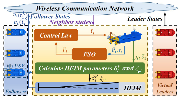
To achieve the stated objectives, this section develops an HEIM-based affine formation control framework (Figure 2). The control law is first constructed to drive the followers toward their desired states. Then, the proposed HEIM is integrated to lower communication energy consumption, ensure a hardware-compatible MCI, and avoid the MII restriction.

3.1. Controller Design

To achieve AFMC, the control law ${\tau }_i$ is constructed as follows:

$$\left\{\begin{array}{cc}\hfill {\tau }_i=& M_i{R}_i^{-1}\left({\psi }_i\right){\tau }_{i0}\hfill \\ \hfill {\tau }_{i0}=& -k_{\eta }\left(\sum _{j\in {\mathcal{V}}_l}{\omega }_{ij}({\eta }_i-{\eta }_j)+\sum _{j\in {\mathcal{V}}_f}{\omega }_{ij}({\eta }_i-{\eta }_j\left(t_{j,k}\right))\right)\hfill \\ \hfill & -k_{\overline{v}}\left(\sum _{j\in {\mathcal{V}}_l}{\omega }_{ij}({\overline{v}}_i-{\overline{v}}_j)+\sum _{j\in {\mathcal{V}}_f}{\omega }_{ij}({\overline{v}}_i-{\overline{v}}_j\left(t_{j,k}\right))\right)-{\widehat{F}}_i,\hfill \end{array}\right.$$

(12)

where $k_{\eta }$ and $k_{\overline{v}}$ are positive control gains, and ${\widehat{F}}_i$ denotes the estimated value of the lumped disturbance $F_i$. The extended state observer (ESO) is designed as follows:

$$\left\{\begin{array}{cc}\hfill & {\dot{\widehat{\overline{v}}}}_i={\widehat{F}}_i+R_i\left({\psi }_i\right)M_i^{-1}{\tau }_i-K_a({\widehat{\overline{v}}}_i-{\overline{v}}_i)\hfill \\ \hfill & {\dot{\widehat{F}}}_i=-K_b({\widehat{\overline{v}}}_i-{\overline{v}}_i)\hfill \end{array}\right.$$

(13)

where $K_a$ and $K_b$ are both diagonal matrices.

3.2. HEIM Design

This section designs a HEIM to reduce interaction energy consumption. Before constructing this mechanism, we first introduce a clock variable for $p\in \{\eta ,\overline{v}\}$:

$$\left\{\begin{array}{c}{\dot{\delta }}_i^p\left(t\right)=\left\{\begin{array}{cc}\min \left\{{\varpi }_i^p\left(t\right),0\right\}-k_0,\hfill & {\delta }_i^p\left(t\right)>0,\parallel {\xi }_{pi}\left(t\right)\parallel \ne 0\hfill \\ -k_0,\hfill & {\delta }_i^p\left(t\right)>0,\parallel {\xi }_{pi}\left(t\right)\parallel =0\hfill \\ 0,\hfill & {\delta }_i^p\left(t\right)=0,\parallel {\xi }_{pi}\left(t\right)\parallel \le {\alpha }_p\hfill \end{array}\right.\hfill \\ t\in (t_i^k,t_i^{k+1})\hfill \\ {\overline{\delta }}_i^p\left(t_i^{k+}\right)={\delta }_0,t=t_i^k\hfill \end{array}\right.$$

(14)

where ${\delta }_0$, $k_0$ and ${\alpha }_p$ are some constants to be designed, ${\xi }_{pi}=p_i-p_i\left(t_i^k\right)$ with $p=\{\eta ,\overline{v}\}$. $t_i^k$ denotes the interaction instant. ${\varpi }_i^p\left(t\right)$ is designed as

$${\varpi }_i^p\left(t\right)={\displaystyle \frac{1}{\parallel {\xi }_{pi}{\left(t\right)\parallel }^2}}-{\left({\delta }_i^p\left(t\right)\right)}^2-1$$

(15)

To determine $t_i^k$, the HEIM is designed as follows:

$$t_i^{k+1}=\inf \left\{\begin{array}{c}t\ge t_i^k|({\delta }_i^{\eta }\left(t\right)\le 0\mathrm{or}{\delta }_i^{\overline{v}}\left(t\right)\le 0)\wedge (\parallel {\xi }_{\eta i}\left(t\right)\parallel \ge {\alpha }_{\eta }\mathrm{or}\parallel {\xi }_{\overline{v}i}\left(t\right)\parallel \ge {\alpha }_{\overline{v}})\hfill \end{array}\right\}$$

(16)

Theorem 1.

Under the proposed HEIM in (16), the interval between two consecutive interactions of each USV is lower bounded by $T_{\min }$, namely,

$$t_i^{k+1}-t_i^k\ge T_{\min }={\displaystyle \frac{\arctan \left({\delta }_0\right./\sqrt{1+k_0})}{\sqrt{1+k_0}}}.$$

(17)

Therefore, Zeno behavior is also naturally excluded.

Proof. 

See Appendix A. □

Remark 3.

The proposed HEIM combines the clock-variable condition with the error-threshold condition. An interaction is triggered only when at least one clock variable ${\delta }_i^p\left(t\right)$ reaches zero and at least one measurement error exceeds its prescribed threshold ${\alpha }_p$, where $p\in \{\eta ,\overline{v}\}$. Since each clock variable requires a strictly positive time to decrease from the reset value ${\delta }_0$ to zero, the clock-variable condition guarantees a positive MCI and excludes Zeno behavior (see Appendix A). In addition, when a clock variable reaches zero, the additional error-threshold condition prevents an interaction from being compulsorily triggered if the measurement errors remain small. This avoids unnecessary interactions triggered solely when the clock variable reaches zero and removes the MII constraint imposed by the clock variable in [23,24,25,26,27,28]. Moreover, compared with MCI-based EIMs [29,30,31,32], the MCI of the proposed HEIM can be actively and flexibly adjusted through the design parameters $k_0$ and ${\delta }_0$, rather than being passively determined by system-related parameters.

Remark 4.

It should be noted that the intermittent updates of neighboring information under the proposed HEIM may cause relatively large variations in the control inputs, thereby increasing actuator activity and mechanical wear. This phenomenon is inherent in event-triggered interaction mechanisms and has also been observed in existing studies [27,31]. For the proposed HEIM, the triggering thresholds ${\delta }_0$ and ${\alpha }_p$ can be appropriately reduced to prevent excessive control variations caused by long inter-event intervals. Alternatively, a low-pass filter or a control-rate constraint can be introduced in future work to smooth the control inputs at triggering instants. These strategies provide a practical trade-off between communication efficiency and control smoothness.

3.3. Stability Analysis

Theorem 2.

Under the proposed controller (12), the tracking error between ${\eta }_f\left(t\right)$ and ${\eta }_f^{*}\left(t\right)$ is uniformly ultimately bounded. Therefore, the follower states ${\eta }_f\left(t\right)$ ultimately converge to a small neighborhood of ${\eta }_f^{*}\left(t\right)$, and the AFMC objective in (11) is achieved.

Proof. 

See Appendix B. □

4. Simulations

4.1. Effectiveness Validation

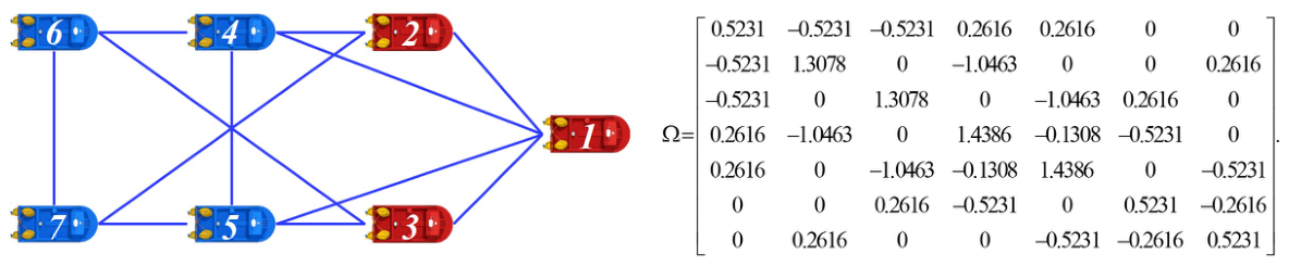
In this section, the effectiveness of the proposed control strategy is verified. The USV cluster shown in Figure 3 is considered, where USVs 1–3 act as leaders and USVs 4–7 act as followers. The values on the edges connecting two nodes represent the corresponding values of the stress matrix. The USV model is from [34]. The initial poses of the USVs are randomly selected as ${\eta }_1\left(0\right)={[16,0,0]}^T$, ${\eta }_2\left(0\right)={[8,8,0]}^T$, ${\eta }_3\left(0\right)={[8,-8,0]}^T$, ${\eta }_4\left(0\right)={[-2,10,0]}^T$, ${\eta }_5\left(0\right)={[-5,-13,0]}^T$, ${\eta }_6\left(0\right)={[-13,15,0]}^T$, and ${\eta }_7\left(0\right)={[-17,-17,0]}^T$. The units are $[\mathrm{m},\mathrm{m},\mathrm{rad}]$. The initial body-fixed velocities are set as ${\vartheta }_i\left(0\right)={[0,0,0]}^T$, $i=1,2,\dots ,7$, with units $[\mathrm{m}/\mathrm{s},\mathrm{m}/\mathrm{s},\mathrm{rad}/\mathrm{s}]$. Moreover, the inertia matrix $M_i$ can be measured in advance, whereas the hydrodynamic matrices $C_i\left({\vartheta }_i\right)$ and $D_i\left({\vartheta }_i\right)$ are assumed to be unknown. The external disturbance acting on the dynamics of the ith USV is selected as $d_{wi}\left(t\right)=0.1\sin \left(0.1t\right)M_i{\mathbf{1}}_3,$ where ${\mathbf{1}}_3={[1,1,1]}^T$. The controller gains are chosen as $k_{\eta }=2$ and $k_{\overline{v}}=4$. The disturbance estimation gains are set as $K_a=\mathrm{diag}(20,20,20)$ and $K_b=\mathrm{diag}(100,100,100)$. The minimum allowable interaction interval (MAII) of the communication hardware is assumed to be $0.04 \mathrm{s}$. For the proposed HEIM, the reset value is selected as ${\overline{\delta }}_i^p\left(t_i^{k+}\right)={\delta }_0=0.1$, with $k_0=1$ and ${\alpha }_p=0.08$. Under these parameters, the guaranteed MCI satisfies $T_{\min }=0.05\mathrm{s}>0.04\mathrm{s}$, which is compatible with the hardware communication capability. If the error-dependent condition $\parallel {\xi }_{\eta i}\left(t\right)\parallel \ge {\alpha }_{\eta }$ and $\parallel {\xi }_{\overline{v}i}\left(t\right)\parallel \ge {\alpha }_{\overline{v}}$ is not incorporated, the communication process is governed only by the reset variable. In this case, the MII is given by $T_{\max }={\delta }_0/k_0=0.1\mathrm{s}$. The simulation time step is set to 0.02 $\mathrm{s}$.

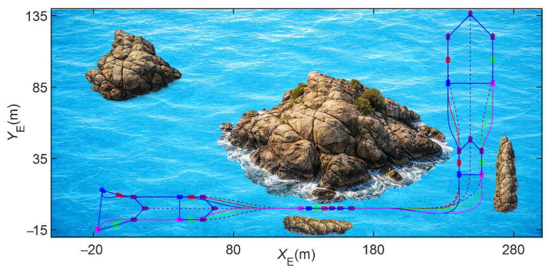
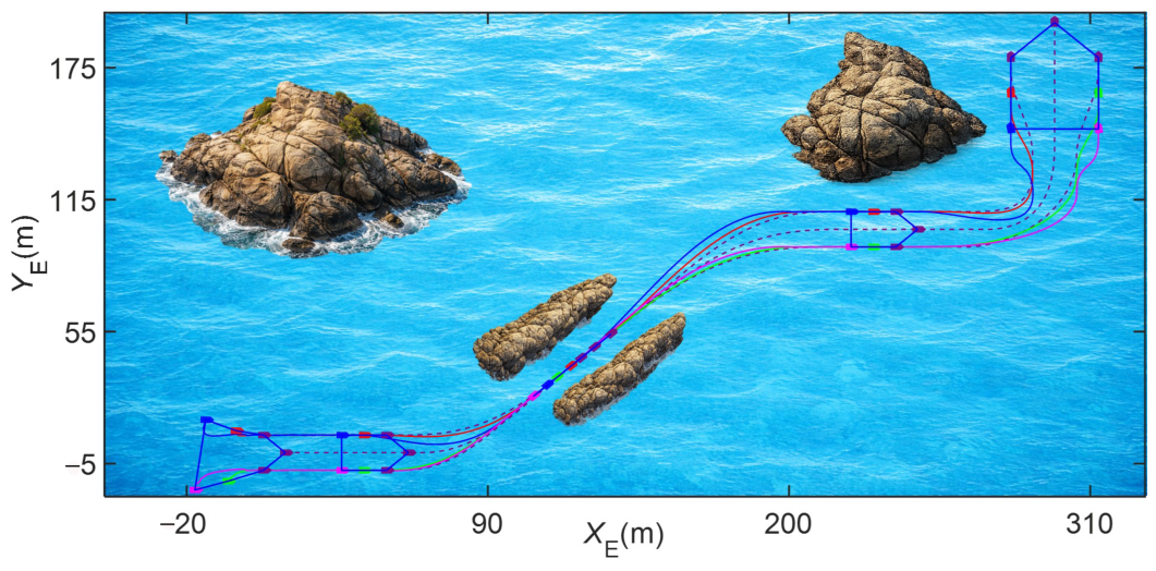
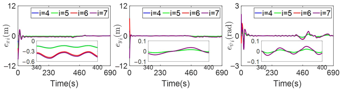
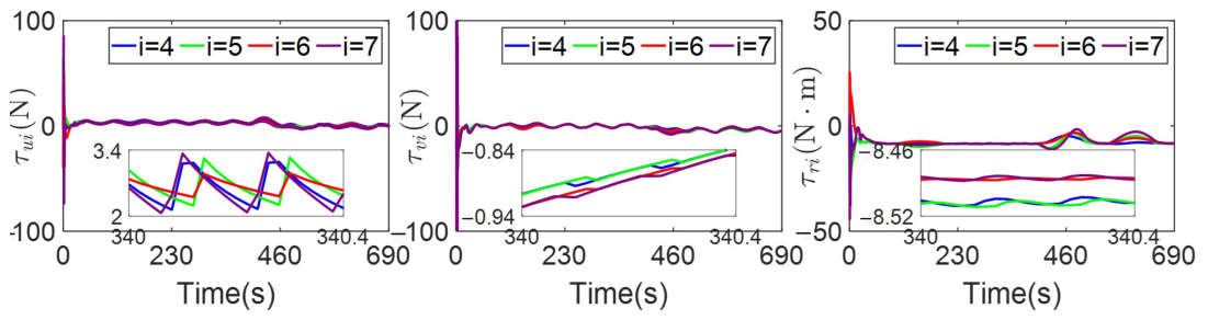
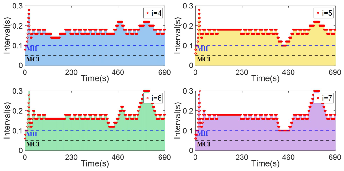
Figure 4, Figure 5, Figure 6, Figure 7 and Figure 8 present the detailed simulation results. Figure 4 and Figure 5 show the motion trajectories of multiple USVs. It can be observed that the USVs gradually form the desired formation and realize coordinated translation, scaling, and rotation. These results demonstrate that the proposed algorithm can achieve affine formation maneuvering rather than only formation keeping. Considering the space limitation, Scenario 1 is taken as an example for further analysis. Figure 6 depicts the position errors and yaw angle errors. It can be observed that these errors finally converge to a small neighborhood of zero, which further validates the effectiveness of the proposed algorithm. Figure 7 illustrates the time evolution of the control inputs. In the initial stage, the control inputs fluctuate significantly due to the large position and velocity errors. As the desired formation is gradually achieved, the control inputs become relatively stable. Figure 8 illustrates the evolution of the interaction intervals over time, where the blue dashed line denotes the maximum interaction interval $T_{\max }$ and the black dashed line denotes the minimum communication interval $T_{\min }$. It can be observed that the interaction instants of USVs 4–7 are non-continuous, which effectively reduces the communication energy consumption. In the initial stage, the large formation errors and drastic formation adjustments lead to frequent interactions and relatively small interaction intervals. Nevertheless, all interaction intervals are always no less than $T_{\min }=0.05\mathrm{s}$, which excludes Zeno behavior and shows that the proposed mechanism is compatible with the hardware communication capacity. Moreover, most interaction intervals can exceed $T_{\max }$. This indicates that the proposed mechanism eliminates unnecessary forced interactions caused by the MII restriction.

4.2. Comparison Results with Existing Strategy

In this section, comparative results are presented to demonstrate the advantages of the proposed HEIM. The EIM proposed in [28] is adopted as the baseline method. For convenience of presentation, it is denoted as EIM0. For a fair comparison, EIM0 is redesigned under the same formation control framework as follows.

$$t_i^{k+1}=\inf \left\{\begin{array}{c}t\ge t_i^k\left|\right(\parallel {\xi }_{\eta i}\left(t\right)\parallel \ge 0.08+0.04\mathrm{acot}\left(0.1t\right)\mathrm{or}\parallel {\xi }_{\overline{v}i}\left(t\right)\parallel \ge 0.08+0.04\mathrm{acot}\left(0.1t\right))\hfill \end{array}\right\}$$

(18)

In addition, the formation error norm is defined as

$$e_{\eta }=\sum _{i\in {\mathcal{V}}_f}\parallel e_{\eta i}\parallel .$$

(19)

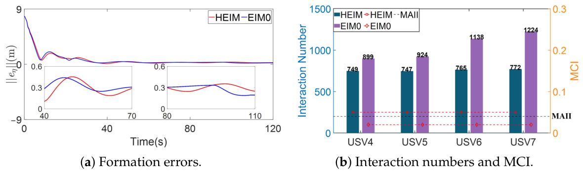
Figure 9 compares the formation error and interaction cost obtained by HEIM and EIM0. It can be observed from Figure 9a that HEIM and EIM0 achieve similar formation maneuvering performance. However, Figure 9b shows that HEIM requires a much lower interaction cost than EIM0. This improvement mainly comes from two aspects. On the one hand, the introduced MCI avoids excessively frequent interactions when the formation errors are large, thereby reducing the risk of communication congestion. On the other hand, benefiting from the MCI-guaranteed interaction design, unnecessary frequent interactions can also be avoided, which further reduces the communication energy consumption. For example, the number of interactions of USV 7 is reduced from 1224 under EIM0 to 772 under HEIM, corresponding to a reduction of 452 interactions, namely about 36.93%. In addition, together with the effectiveness validation results, it can be further observed that HEIM removes the MII constraint. Therefore, the proposed HEIM not only reduces the interaction cost but also avoids MII restriction, which further confirms its advantages.

5. Conclusions

This paper proposes a HEIM with an adjustable MCI for AFMC of USVs. By introducing a clock variable, the proposed HEIM guarantees a hardware-compatible MCI and prevents excessively frequent interactions. Moreover, an additional threshold is incorporated into the interaction condition to avoid forced interactions caused solely by the clock variable, thereby removing the MII and improving communication efficiency. Theoretical analysis proved that the AFMC objective can be achieved and that Zeno behavior is excluded. Simulation results further verified the effectiveness of the proposed method. However, communication delays are not considered in the current framework, which may degrade the control performance. In addition, only undirected communication topologies are considered. Future work will extend the proposed method to delay-affected marine communication networks with directed topologies.

References

1. Wang, Z.; Jiang, S.; Xue, Y.; Mu, X.; Wang, C. Fixed-Time Event-Triggered Fault-Tolerant Formation Control for Autonomous Underwater Vehicle Swarms. J. Mar. Sci. Eng. 2025, 13, 2249. [Google Scholar] [CrossRef]
2. Wang, H.; Wang, H.; Guo, X. Distributed Adaptive Fault-Tolerant Formation Control for Heterogeneous USV-AUV Swarms Based on Dynamic Event Triggering. J. Mar. Sci. Eng. 2025, 13, 2116. [Google Scholar] [CrossRef]
3. Peng, Z.; Wang, C.; Yin, Y.; Wang, J. Safety-Certified Constrained Control of Maritime Autonomous Surface Ships for Automatic Berthing. IEEE Trans. Veh. Technol. 2023, 72, 8541–8552. [Google Scholar] [CrossRef]
4. Lin, Y.; Jia, Z.; Guo, D.; Zhang, W. Dynamic Performance-Guaranteed Adaptive Event-Triggered Trajectory Tracking Control for Underactuated Surface Vehicles. Ocean Eng. 2024, 312, 119114. [Google Scholar] [CrossRef]
5. Yao, M.; Guo, K.; Lu, Y.; Zhang, W.; Qiao, L. Distributed Adaptive Integral Sliding Mode Affine Formation Maneuver Control for Multiple AUVs With Event-Triggered Chattering-Reduction Mechanism. IEEE Trans. Veh. Technol. 2024, 73, 16341–16350. [Google Scholar] [CrossRef]
6. He, S.; Dai, S.-L.; Zhao, Z.; Zou, T.; Ma, Y. UDE-Based Distributed Formation Control for MSVs With Collision Avoidance and Connectivity Preservation. IEEE Trans. Ind. Inform. 2024, 20, 1476–1487. [Google Scholar] [CrossRef]
7. Zhu, C.; Song, Y.; Huang, B. Edge Weighted-Based Formation Control for Unmanned Surface Vehicles: Stochastic Collision Avoidance with Parameterized Convergence Time. IEEE/CAA J. Autom. Sin. 2026; in press. [CrossRef]
8. Huang, B.; Peng, H.; Ahn, C.K. Noncooperative Game-Based Probability Assignment Formation Control for Networked Unmanned Surface Vehicles under Stochastic Packet Losses. IEEE Trans. Autom. Sci. Eng. 2026; in press. [CrossRef]
9. Zhu, W.; Xia, G.; Jiang, X. A Design of Leaderless Formation Controller for Multi-ASVs with Sampled Data and Communication Delay. J. Mar. Sci. Eng. 2025, 13, 1259. [Google Scholar] [CrossRef]
10. Jia, Z.; Lu, H.; Chen, H.; Zhang, W. Robust Distributed Cooperative Rendezvous Control for Heterogeneous Marine Vehicles Using Model Predictive Control. IEEE Trans. Veh. Technol. 2024, 73, 11002–11013. [Google Scholar] [CrossRef]
11. Wang, X.; Pang, N.; Xu, Y.; Huang, T.; Kurths, J. On State-Constrained Containment Control for Nonlinear Multiagent Systems Using Event-Triggered Input. IEEE Trans. Syst. Man Cybern. Syst. 2024, 54, 2530–2538. [Google Scholar] [CrossRef]
12. Wang, X.; Guang, W.; Huang, T.; Kurths, J. Optimized Adaptive Finite-Time Consensus Control for Stochastic Nonlinear Multiagent Systems With Non-Affine Nonlinear Faults. IEEE Trans. Autom. Sci. Eng. 2024, 21, 5012–5023. [Google Scholar] [CrossRef]
13. Aranda, M.; López-Nicolás, G.; Sagüés, C.; Mezouar, Y. Coordinate-Free Formation Stabilization Based on Relative Position Measurements. Automatica 2015, 57, 11–20. [Google Scholar] [CrossRef]
14. De Marina, H.G.; Jayawardhana, B.; Cao, M. Distributed Rotational and Translational Maneuvering of Rigid Formations and Their Applications. IEEE Trans. Robot. 2016, 32, 684–697. [Google Scholar] [CrossRef]
15. Lu, Y.; Wen, C.; Shen, T.; Zhang, W. Bearing-Based Adaptive Neural Formation Scaling Control for Autonomous Surface Vehicles with Uncertainties and Input Saturation. IEEE Trans. Neural Netw. Learn. Syst. 2021, 32, 4653–4664. [Google Scholar] [CrossRef] [PubMed]
16. Fan, Z.; Xu, Y.; Fu, M.; Liu, Y.; Dong, L.; Yang, J. Similar Formation Maneuver Control of Multi-ASV Systems via Complex Laplacian and Global Orientation Estimation. IEEE Trans. Veh. Technol. 2026. early access. [Google Scholar] [CrossRef]
17. Xu, Y.; Luo, D.; Li, D.; You, Y.; Duan, H. Affine Formation Control for Heterogeneous Multi-Agent Systems with Directed Interaction Networks. Neurocomputing 2019, 330, 104–115. [Google Scholar] [CrossRef]
18. Huang, B.; Zhu, C.; Xu, Y.; Zhu, G.; Su, Y. Energy Tradeoff-Oriented Quasi-Optimal Distributed Affine Formation Maneuver Control for Electric Marine Surface Vehicles. IEEE Trans. Transp. Electrif. 2025, 11, 2019–2034. [Google Scholar] [CrossRef]
19. Fan, Z.; Xu, Y.; Fu, M.; Zhang, W.; Zhang, G.; Wang, J. Two-Layer Affine Formation Maneuvering Control of Multi-Hovercraft with Connectivity Maintenance and Collision Avoidance. Ocean Eng. 2025, 320, 120232. [Google Scholar] [CrossRef]
20. Huang, B.; Zhou, X.; Zhang, C.; Ahn, C.K. Event-Triggered L2 Performance Control for Affine Formation of Networked Unmanned Surface Vehicles with Intermittent Communication. IEEE Trans. Intell. Transp. Syst. 2025, 26, 962–973. [Google Scholar] [CrossRef]
21. Tang, C.; Zhang, H.-T.; Cao, H.; Wang, J. Time-Varying Formation Control of Autonomous Surface Vehicles Based on Affine Observer. IEEE Trans. Ind. Electron. 2024, 71, 11604–11615. [Google Scholar] [CrossRef]
22. Zhang, Y.; Miao, J.; Huang, B.; Lin, J. Reliability-Enhanced Affine Formation Maneuver Control for Underactuated Unmanned Marine Vehicles Under Random Packet Losses. IEEE Internet Things J. 2026, 13, 13720–13733. [Google Scholar] [CrossRef]
23. Lv, M.; Peng, Z.; Wang, D.; Han, Q.-L. Event-Triggered Cooperative Path Following of Autonomous Surface Vehicles over Wireless Network with Experiment Results. IEEE Trans. Ind. Electron. 2022, 69, 11479–11489. [Google Scholar] [CrossRef]
24. Wang, Z.; Zhang, A.; Qin, H.; Jiang, S. Fixed-Time Average Consensus of a Dynamic Event-Triggered Mechanism in a System of Multiple Underactuated Autonomous Underwater Vehicles Based on a Body Frame Spherical Coordinate System. J. Mar. Sci. Eng. 2023, 11, 385. [Google Scholar] [CrossRef]
25. Zhang, G.; Liu, S.; Zhang, X.; Zhang, W.-D. Event-Triggered Cooperative Formation Control for Autonomous Surface Vehicles under the Maritime Search Operation. IEEE Trans. Intell. Transp. Syst. 2022, 23, 21392–21404. [Google Scholar] [CrossRef]
26. Jiang, X.; Xia, G. Event-Triggered Practical Formation Control of Leaderless Unmanned Surface Vehicles with Environmental Disturbances. IEEE Trans. Circuits Syst. II Express Briefs 2024, 71, 1326–1330. [Google Scholar] [CrossRef]
27. Zhu, C.; Huang, B.; Lu, Y.; Li, X.; Su, Y. Distributed Affine Formation Maneuver Control of Autonomous Surface Vehicles with Event-Triggered Data Transmission Mechanism. IEEE Trans. Control Syst. Technol. 2023, 31, 2045–2058. [Google Scholar] [CrossRef]
28. Zhang, Y.; Miao, J.; Huang, B. Dual-Layer Dynamic Event-Triggered Formation Maneuver Control for Underactuated Autonomous Underwater Vehicles via Edge Vector-Based Method. Ocean Eng. 2025, 330, 121200. [Google Scholar] [CrossRef]
29. Qian, Y.-Y.; Wan, Y. Design of Distributed Adaptive Event-Triggered Consensus Control Strategies with Positive Minimum Inter-Event Times. Automatica 2021, 133, 109837. [Google Scholar] [CrossRef]
30. Long, J.; Wang, W.; Guo, Y.; Liu, Z. Chattering Free Distributed Event-Triggered Adaptive Attitude Synchronization of Multiple Spacecraft With Positive Minimum Interevent Times. IEEE Trans. Control Netw. Syst. 2025, 12, 374–386. [Google Scholar] [CrossRef]
31. Cui, H.; Zhao, G.; Liu, S.; Li, Z. A Novel Adaptive Event-Triggered Consensus Control Approach to Multi-Agent Systems With Guaranteed Positive MIET. IEEE Trans. Netw. Sci. Eng. 2024, 11, 270–283. [Google Scholar] [CrossRef]
32. Zhou, B.; Huang, B.; Mao, L.; Zhu, C.; Su, Y. Distributed Observer Based Event-Triggered Affine Formation Maneuver Control for Underactuated Surface Vessels with Positive Minimum Inter-Event Times. Int. J. Robust Nonlinear Control 2022, 32, 7712–7732. [Google Scholar] [CrossRef]
33. Huang, B.; Ren, X.; Zhou, B.; Zhang, Z.; Zhou, X.; Miao, J. An Intermittent Anti-Competition Communication Mechanism-Based Formation Maneuvers for Internet of Unmanned Surface Vehicles. IEEE Internet Things J. 2025, 12, 3234–3247. [Google Scholar] [CrossRef]
34. Zhang, Y.; Wang, S.; Wang, X.; Tian, X. Bearing-Based Formation Control for Multiple Underactuated Autonomous Surface Vehicles with Flexible Size Scaling. Ocean Eng. 2023, 267, 113242. [Google Scholar] [CrossRef]
35. Zhang, Y.; Miao, J.; Lin, J.; Huang, B. Affine Formation Maneuver Control for NUMVs Under Unreliable Networks: A Reliability-Enhanced Interaction Strategy. IEEE Trans. Autom. Sci. Eng. 2026, 23, 9845–9857. [Google Scholar] [CrossRef]
Figure 1. Coordinates and motions of USVs.
Symmetry 18 01277 g001
Figure 2. The proposed HEIM-based formation control strategy for USVs.
Symmetry 18 01277 g002
Figure 3. Nominal formation and stress matrix of the USV system.
Symmetry 18 01277 g003
Figure 4. Time-varying trajectories of USVs under the proposed strategy in Scenario 1.
Symmetry 18 01277 g004
Figure 5. Time-varying trajectories of USVs under the proposed strategy in Scenario 2.
Symmetry 18 01277 g005
Figure 6. Formation errors in different directions under the proposed strategy.
Symmetry 18 01277 g006
Figure 7. Control inputs of USVs under the proposed strategy.
Symmetry 18 01277 g007
Figure 8. Interaction intervals of USVs under the proposed strategy.
Symmetry 18 01277 g008
Figure 9. Formation error and interaction cost of the USVs under two EIMs: (a) formation errors; (b) interaction numbers and MCI.
Symmetry 18 01277 g009
Disclaimer/Publisher’s Note: The statements, opinions and data contained in all publications are solely those of the individual author(s) and contributor(s) and not of MDPI and/or the editor(s). MDPI and/or the editor(s) disclaim responsibility for any injury to people or property resulting from any ideas, methods, instructions or products referred to in the content.