Enhanced Computational Efficiency in Solving Delay Fractional Partial Differential Equations Through the Yang Decomposition Method

Abstract

This study presents the Yang Transform Adomian Decomposition Method (YTADM), a semi-analytical framework for solving one-dimensional linear and nonlinear delay fractional partial differential equations involving the Caputo fractional derivative. The proposed method combines the Yang transform with the Adomian decomposition method to construct recursive solution series while efficiently handling delayed nonlinear terms. The applicability of the proposed framework is demonstrated through several examples, including proportional-delay Burgers-type equations, and its convergence properties are analyzed. The obtained results show that YTADM yields rapidly convergent semi-analytical approximations and provides an effective framework for solving one-dimensional delay fractional partial differential equations.

1. Introduction

Fractional partial differential equations (FPDEs) have been studied extensively, since fractional-order models better describe a wide variety of complex physical phenomena than traditional integer-order PDE models. Fractional derivative theory is being used to model diverse scientific and technical applications [1,2,3].

In addition, delay fractional differential equations represent an additional subclass of models. Since many systems respond to their past states rather than current condition alone, delay terms provide an accurate representation of this behavior. Examples of such delays include maturations, feedback lags, memory responses, and propagation times in biological systems, mechanical systems, control systems, and mass transport systems [4,5,6,7]. Combining fractional derivatives with delay terms provides a mathematical framework capable of modeling both distributed memory and explicit retardation.

Several researchers have contributed to the theoretical and computational analysis of fractional delay PDEs. For example, Ouyang [8] proved the existence and uniqueness of solutions for nonlinear fractional-order PDE’s with delay. Rihan [9] developed computational methods for delay parabolic and time-fractional PDE’s. Prakash et al. [10] derived an exact solution for nonlinear time-fractional reaction–diffusion PDE’s with delay. Benchmark results to compare against exact solutions were provided. Additionally, the author of [11] demonstrated the application of fractional delay differential equations with non-singular kernels to model hand-foot-and-mouth disease. Therefore, they have proven useful in epidemiological studies.

A variety of analytical and numerical methods have been developed in order to solve fractional differential equations, including Laplace transform-based decomposition to solve linear Volterra integro-fractional differential equations with delay and symbolic Laplace transform techniques to solve delay differential equations [12,13]. Other authors have found exact solutions using the Laplace transform [14,15] and developed Laplace transform-based homotopy-type methods.

Additionally, several authors have used other transforms to develop novel methods for finding solutions to fractional PDEs. Nurudeen et al. [16] used the Aboodh transform combined with the Adomian Decomposition Method to derive analytical solutions for time-fractional heat diffusion equations. Merdan et al. [17] applied the Aboodh–Adomian decomposition method to Caputo–Fabrizio fractional differential equations. Al-Aati and Al-Sharai [18] proposed a double Aboodh–Shehu decomposition method for solving linear and nonlinear coupled partial differential equations. Noor et al. [19] introduced the Aboodh residual power series method and Aboodh transform iteration method for fractional-order PDEs. Ali and Merdan [20,21] employed the Yang Transform Adomian Decomposition Method to derive approximate analytical solutions for nonlinear time-fractional coupled Burgers and Swift–Hohenberg.

Other transform-based methods have also been explored. Natural transform-based methods have been combined with decomposition techniques to solve fractional PDEs with delay in [22,23,24]. Alsulami et al. [25] proposed an effective iterative procedure using the Sumudu decomposition method for delay fractional partial differential equations. In [26,27,28], the authors proposed numerical schemes for fractional delay differential equations. Moreover, spectral and advanced numerical schemes have been developed in recent years in [29,30,31], which significantly improved the computational speed and accuracy. Liaqat et al. [32] proposed a new numerical method for solving fractional ordinary differential equations with proportional delay. Meanwhile, Sabermahani et al. [33] developed a Fibonacci-hybrid function approach for solving fractional delay differential equations.

Recently, hybrid transform–decomposition methods have emerged as efficient and practical methods for solving various types of FDEs. For example, Ganie et al. [34,35] utilized Elzaki–Yang transforms and ADM-Homotopy Perturbation Methods for solving fractional dispersive and reaction–diffusion PDEs. Abdali et al. [36] presented a combination of ADM and Yasser–Jassim Transform. Ramadan et al. [37] proposed an accelerated version of the Laplace–ADM technique for solving time-fractional nonlinear PDEs. Şahin et al. [38] developed a hybrid approach using q-HAM and Shehu’s transformations to approximate solutions to the Newell–Whitehead–Segel equation. Al-Griffi and Al-Saif [39] applied Yang transform based Homotopy Perturbation Methods to Non-Newtonian viscoelastic fluid flow problems. Locally Fractional Decomposition Methods were also developed by Merdan and Oral [40].

Homotopy Perturbation and Variational Iteration Methods have also been employed to solve FDPDEs. Singh and Kumar [41,42,43], employed Homotopy Perturbation and Variational Iteration Methods to solve fractional delay partial differential equations.

The paper presents the Yang Transform Adomian Decomposition Method (YTADM) for solving fractional delay partial differential equations (FDPDEs) involving Caputo fractional derivatives. Both linear and nonlinear FDPDEs are considered, including models with constant-delay, proportional-delay, and Burgers-type nonlinearities. The main objective of this study is to develop a systematic YTADM-based framework for constructing rapidly convergent semi-analytical solutions for one-dimensional delay fractional partial differential equations. Although transform-based decomposition methods have been successfully employed to solve various fractional differential equations, a unified analytical framework capable of treating both constant-delay and proportional-delay fractional partial differential equations within a single formulation has not been systematically addressed in the literature. The proposed YTADM exploits the operational properties of the Yang transform for Caputo fractional derivatives to derive a simple recursive algorithm that naturally incorporates the prescribed initial conditions while accommodating delayed linear and nonlinear terms without additional interpolation. Furthermore, the benchmark problems considered in this work are newly constructed with nonhomogeneous source terms chosen to admit exact closed-form solutions, enabling rigorous verification of the proposed method through direct comparison with exact solutions. The effectiveness of the proposed framework is demonstrated through several examples together with theoretical convergence analysis.

The rest of the paper is structured as follows: Section 2 describes some fundamental characteristics of the Yang transform and Caputo fractional derivatives. The methodology of YTADM is described in Section 3. In Section 4, convergence analysis is performed. Applications are shown in Section 5. The results and discussion are presented in Section 6. Lastly, conclusions are presented in Section 7.

2. Preliminary Concepts

In this section, we present the basic properties and definitions of the Yang transform and the Caputo fractional derivative that will be employed in this study.

Definition 1

([44,45]). The Yang transform (YT) is defined as

$$\mathsf{Y}\left[\Theta \left(\xi \right)\right]\left(\chi \right)={\int }_0^{\infty }{e}^{-{\displaystyle \frac{\xi }{\chi }}}\Theta \left(\xi \right)d\xi =\mathcal{R}\left(\chi \right),\chi >0,$$

(1)

while the inverse Yang transform is given by ${\mathsf{Y}}^{-1}\left[\mathcal{R}\left(\chi \right)\right]=\Theta \left(\xi \right)$.

Theorem 1

(Existence conditions [46]). Let $\Theta \left(\xi \right)$ be a piecewise continuous function on the interval $[0,\infty )$ and of exponential order q; that is,

$$\left|\Theta \left(\xi \right)\right|\le M{e}^{q\xi },$$

where $M>0$ and $q>0$ are constants. Then, the Yang transform

$$\mathsf{Y}\left[\Theta \left(\xi \right)\right]={\int }_0^{\infty }{e}^{-\xi /\chi }\Theta \left(\xi \right)d\xi \mathit{exists}\mathit{for}{\displaystyle \frac{1}{\chi }}>q.$$

Proof. 

Using the Definition 1, we obtain

$$\begin{array}{cc}\hfill \left|\mathsf{Y}\right[\Theta \left(\xi \right)\left]\right|& =\left|{\int }_0^{\infty }{e}^{-\xi /\chi }\Theta \left(\xi \right)d\xi \right|\le {\int }_0^{\infty }{e}^{-\xi /\chi }\left|\Theta \left(\xi \right)\right|d\xi \hfill \\ \hfill & \le M{\int }_0^{\infty }{e}^{-\xi /\chi }{e}^{q\xi }d\xi =M{\int }_0^{\infty }{e}^{-\left({\displaystyle \frac{1}{\chi }}-q\right)\xi }d\xi ={\displaystyle \frac{M}{\frac{1}{\chi }-q}};\hfill \end{array}$$

(2)

therefore, the Yang transform exists for ${\displaystyle \frac{1}{\chi }}>q$. □

Remark 1.

The following defines the Yang transformation of a few useful functions

$$\begin{array}{c}\hfill \mathsf{Y}\left[1\right]=\chi ,\mathsf{Y}\left[\xi \right]={\chi }^2,\mathsf{Y}\left[{\xi }^{\eta }\right]=\Gamma (\eta +1){\chi }^{\eta +1},\eta \ge 0.\end{array}$$

Definition 2

([44,45]). Let $\Theta (\mu ,\xi )$ be sufficiently smooth with respect to ξ. The Caputo fractional derivative of η is defined as

$${}^{C}D_{\xi }^{\eta }\Theta (\mu ,\xi )=\left\{\begin{array}{cc}{\displaystyle {\displaystyle \frac{1}{\Gamma (k-\eta )}}{\int }_0^{\xi }{(\xi -\sigma )}^{k-\eta -1}{\Theta }^{\left(k\right)}(\mu ,\sigma )d\sigma ,}\hfill & k-1<\eta \le k,\hfill \\ {\displaystyle \frac{{\partial }^n}{\partial {\xi }^n}}\Theta (\mu ,\xi )\hfill & \eta =n\in \mathbb{N}.\hfill \end{array}\right.$$

(3)

Proposition 1

([44,45]). The Yang transform of the $n^{th}$ derivative is defined as

$$\mathsf{Y}\left[{\Theta }^{\left(n\right)}\left(\xi \right)\right]={\displaystyle \frac{\mathcal{R}\left(\chi \right)}{{\chi }^n}}-{\displaystyle \sum _{r=0}^{n-1}}{\displaystyle \frac{{\Theta }^{\left(r\right)}\left(0\right)}{{\chi }^{n-(r+1)}}}.$$

(4)

Proposition 2

([44,45]). The Yang transform of the Caputo fractional derivative is defined as

$$\mathsf{Y}\left[{}^{C}D_{\xi }^{\eta }\Theta (\mu ,\xi )\right]={\displaystyle \frac{\mathcal{R}(\mu ,\chi )}{{\chi }^{\eta }}}-{\displaystyle \sum _{r=0}^{n-1}}{\displaystyle \frac{{\Theta }^{\left(r\right)}(\mu ,0)}{{\chi }^{\eta -(r+1)}}},n-1<\eta \le n,n\in \mathbb{N}.$$

(5)

Remark 2.

Under the hypotheses of Theorem 1, $\Theta \left(\xi \right)$ is piecewise continuous on $[0,\infty )$ and of exponential order, and the Yang transform exists. So, whenever $\mathcal{R}\left(\chi \right)=\mathsf{Y}\left[\Theta \right(\xi \left)\right]$, the inverse Yang transform ${\mathsf{Y}}^{-1}\left[\mathcal{R}\left(\chi \right)\right]$ is well defined.

3. Methodology

This section presents the application of the Yang Transform Adomian Decomposition Method (YTADM) to a general form of non-homogeneous nonlinear fractional partial differential equations (FPDEs).

$${}^{C}D_{\xi }^{\eta }\Theta (\mu ,\xi )+\mathbf{T}\Theta (\mu ,\xi )+\mathbf{S}\Theta (\mu ,\xi )={{\rm Y}}_1(\mu ,\xi ),$$

(6)

with the initial condition

$$\Theta (\mu ,0)={{\rm Y}}_2\left(\mu \right).$$

(7)

where ${}^{C}D_{\xi }^{\eta }\Theta$ denotes the Caputo fractional derivative of order $\eta$, with $0<\eta \le 1$, and $\eta$ represents the fractional order throughout this paper. The operators $\mathbf{T}$ and $\mathbf{S}$ are linear and nonlinear operators, respectively, ${{\rm Y}}_1(\mu ,\xi )$ is the nonhomogeneous source function, and $\mu$ and $\xi$ are the variables representing space and time, respectively. Applying the Yang transform to Equation (6) yields

$$\mathsf{Y}[{}^{C}D_{\xi }^{\eta }\Theta (\mu ,\xi )+\mathbf{T}\Theta (\mu ,\xi )+\mathbf{S}\Theta (\mu ,\xi )]=\mathsf{Y}\left[{{\rm Y}}_1(\mu ,\xi )\right],$$

$${\displaystyle \frac{\mathcal{R}(\mu ,\xi )}{{\chi }^{\eta }}}-{\displaystyle \frac{\Theta (\mu ,0)}{{\chi }^{\eta -1}}}+\mathsf{Y}[\mathbf{T}\Theta (\mu ,\xi )+\mathbf{S}\Theta (\mu ,\xi )]=\mathsf{Y}\left[{{\rm Y}}_1(\mu ,\xi )\right],$$

$$\mathcal{R}(\mu ,\xi )=\chi \Theta (\mu ,0)+{\chi }^{\eta }\mathsf{Y}[{{\rm Y}}_1(\mu ,\xi )-\mathbf{T}\Theta (\mu ,\xi )-\mathbf{S}\Theta (\mu ,\xi )].$$

(8)

Applying the inverse Yang transform to Equation (8), we have

$$\Theta (\mu ,\xi )=\Theta (\mu ,0)+{\mathsf{Y}}^{-1}\left[{\chi }^{\eta }\mathsf{Y}\right[{{\rm Y}}_1(\mu ,\xi )-\mathbf{T}\Theta (\mu ,\xi )-\mathbf{S}\Theta (\mu ,\xi )\left]\right].$$

(9)

Assume that

$$\Theta (\mu ,\xi )={\displaystyle \sum _{n=0}^{\infty }}{\Theta }_n(\mu ,\xi ),\mathbf{S}\Theta (\mu ,\xi )={\displaystyle \sum _{n=0}^{\infty }}{\mathcal{U}}_n,$$

(10)

where ${\mathcal{U}}_n$ is ADM, defined by

$${\mathcal{U}}_n={\displaystyle \frac{1}{n!}}{\left.{\displaystyle \frac{{\partial }^n}{\partial {\lambda }^n}}\mathbf{S}\left({\displaystyle \sum _{k=0}^{\infty }}{\lambda }^k{\Theta }_k\right)\right|}_{\lambda =0},n\ge 0.$$

(11)

Substituting Equation (10) into Equation (9) results in

$${\displaystyle \sum _{n=0}^{\infty }}{\Theta }_n(\mu ,\xi )=\Theta (\mu ,0)+{\mathsf{Y}}^{-1}\left[{\chi }^{\eta }\mathsf{Y}\right[{{\rm Y}}_1(\mu ,\xi )\left]\right]-{\mathsf{Y}}^{-1}\left[{\chi }^{\eta }\mathsf{Y}\right[\mathbf{T}\left({\displaystyle \sum _{n=0}^{\infty }}{\Theta }_n(\mu ,\xi )\right)+{\displaystyle \sum _{n=0}^{\infty }}{\mathcal{U}}_n\left]\right].$$

(12)

Equating both sides of Equation (12), we have the following:

$$\left\{\begin{array}{c}{\Theta }_0(\mu ,\xi )=\Theta (\mu ,0)+{\mathsf{Y}}^{-1}\left[{\chi }^{\eta }\mathsf{Y}\right[{{\rm Y}}_1(\mu ,\xi )\left]\right],\hfill \\ {\Theta }_1(\mu ,\xi )=-{\mathsf{Y}}^{-1}\left[{\chi }^{\eta }\mathsf{Y}\right[\mathbf{T}\left({\Theta }_0(\mu ,\xi )\right)+{\mathcal{U}}_0\left]\right],\hfill \\ ⋮\hfill \\ {\Theta }_{n+1}(\mu ,\xi )=-{\mathsf{Y}}^{-1}\left[{\chi }^{\eta }\mathsf{Y}\right[\mathbf{T}\left({\Theta }_n(\mu ,\xi )\right)+{\mathcal{U}}_n\left]\right],n\ge 1.\hfill \end{array}\right.$$

(13)

Therefore, the YTADM solution is given by

$$\Theta (\mu ,\xi )={\displaystyle \sum _{n=0}^{\infty }}{\Theta }_n={\Theta }_0(\mu ,\xi )+{\Theta }_1(\mu ,\xi )+{\Theta }_2(\mu ,\xi )+\cdots$$

(14)

4. Convergence Analysis

In this part, we prove the existence and the convergence theorems for the series solutions found by the Yang Transform Adomian Decomposition Method (YTADM) for the nonlinear FDEs. Let us define the Banach space $C[0,T]$ as the space of all continuous functions on $[0,T]$ and equip it with the sup-norm. We consider the function $\Theta (\mu ,\xi )$ and ${\Theta }_n(\mu ,\xi )\in C[0,T]$.

Theorem 2

(Theorem of Uniqueness [47,48]). The unique solution to the nonlinear FPDEs of Equation (6) found by YTADM is valid for $0<\delta <1$.

Proof. 

The recursive YTADM formulation for the nonlinear FPDEs of Equation (6) is given by

$$\left\{\begin{array}{cc}\hfill & {\Theta }_0(\mu ,\xi )=\Theta (\mu ,0)={{\rm Y}}_2\left(\mu \right),n=0,\hfill \\ \hfill & {\displaystyle {\Theta }_{n+1}(\mu ,\xi )={\mathsf{Y}}^{-1}\left[{\chi }^{\eta }\mathsf{Y}\left[{{\rm Y}}_1(\mu ,\xi )\right]\right]-{\mathsf{Y}}^{-1}\left\{{\chi }^{\eta }\mathsf{Y}\left[\mathbf{T}\left({\displaystyle \sum _{n=0}^{\infty }}{\Theta }_n(\mu ,\xi )\right)+{\displaystyle \sum _{n=0}^{\infty }}{\mathcal{U}}_n\right]\right\},n\ge 0.}\hfill \end{array}\right.$$

(15)

Consider the two distinct solutions of YTADM for the nonlinear FDE (6). The solutions are denoted by $\Theta (\mu ,\xi )$ and $\Phi (\mu ,\xi )$, and both satisfy the inequality $\left|\Theta \right|\le \sigma$ and $|\Phi |\le \sigma$. Then, we can derive

$$\left|\Theta (\mu ,\xi )-\Phi (\mu ,\xi )\right|=\left|{\mathsf{Y}}^{-1}\left({\chi }^{\eta }\mathsf{Y}\left[\mathbf{T}(\Theta -\Phi )+\mathbf{S}(\Theta -\Phi )\right]\right)\right|.$$

(16)

Applying Yang transform’s convolution property implies that

$$\begin{array}{cc}\hfill \left|\Theta (\mu ,\xi )-\Phi (\mu ,\xi )\right|& \le {\int }_0^{\xi }\left|\left(\mathbf{T}\Theta -\mathbf{T}\Phi \right)+\left(\mathbf{S}\Theta -\mathbf{S}\Phi \right)\right|{\displaystyle \frac{{(\xi -\mu )}^{\eta }}{\Gamma (\eta +1)}}d\mu \hfill \\ \hfill & \le {\int }_0^{\xi }\left(\left|\mathbf{T}\left(\Theta \right)-\mathbf{T}(\Phi )\right|+\left|\mathbf{S}\left(\Theta \right)-\mathbf{S}(\Phi )\right|\right){\displaystyle \frac{{(\xi -\mu )}^{\eta }}{\Gamma (\eta +1)}}d\mu ,\hfill \end{array}$$

(17)

where $\mathbf{T}$ is bounded, i.e., $\left|\mathbf{T}\right(\Theta )-\mathbf{T}(\Phi \left)\right|\le \vartheta |\Theta -\Phi |$, and the nonlinear operator $\mathbf{S}$ satisfies the Lipschitz condition with $\kappa >0$ such that $\left|\mathbf{S}\right(\Theta )-\mathbf{S}(\Phi \left)\right|\le \kappa |\Theta -\Phi |$

$$|\Theta -\Phi |\le {\int }_0^{\xi }(\vartheta +\kappa )\left|\right|\Theta -\Phi \left|\right|{\displaystyle \frac{{(\xi -\mu )}^{\eta }}{\Gamma (\eta +1)}}d\mu .$$

(18)

From the integral mean value theorem, it follows that

$$|\Theta -\Phi |\le \left((\vartheta +\kappa )\left|\right|\Theta -\Phi \left|\right|\right)MT,$$

(19)

where ${\displaystyle M=\underset{\xi \in I}{max}\frac{{(\xi -\mu )}^{\eta }}{\Gamma (\eta +1)}}$, and $\xi \in (0,T)$. Hence, $|\Theta -\Phi |\le \delta |\Theta -\Phi |$, where $\delta =(\vartheta +\kappa )MT$. So, $(1-\delta )|\Theta -\Phi |\le 0$, which implies that $\Theta =\Phi$, whenever $\delta \in (0,1)$. Consequently, the solution is unique. □

Theorem 3

(Convergence Theorem [48,49]). Let N be a Banach space and $U:N\to N$ be a nonlinear mapping. Then, the following inequality holds:

$$\parallel U\left(\Theta \right)-U(\Phi )\parallel \le \delta \parallel \Theta -\Phi \parallel ,\forall \Theta ,\Phi \in N.$$

(20)

By Banach’s fixed point theorem, U has a unique fixed point [17] if it exists. Furthermore, the $\left\{{\Theta }_n\right\}$ sequence generated by YTADM converges to this fixed point for the arbitrary initial choices ${\Theta }_0,{\Theta }_1\in N$. In particular,

$$\parallel {\Theta }_m-{\Theta }_n\parallel \le {\displaystyle \frac{{\delta }^n}{1-\delta }}\parallel {\Theta }_1-{\Theta }_0\parallel .$$

(21)

Proof. 

Assume that a Banach space $\left(C\right[I],\parallel ·\parallel )$ contains all continuous functions on $I=[0,T]$, and the norm is defined as ${\displaystyle \parallel p\parallel =\underset{\xi \in I}{max}\left|p\left(\sigma \right)\right|}$. Now, we demonstrate that the sequence ${\Theta }_n$ is a Cauchy sequence in the Banach space:

$$\begin{array}{cc}\hfill \parallel {\Theta }_m-{\Theta }_n\parallel & {\displaystyle =\underset{\xi \in I}{max}|{\Theta }_m-{\Theta }_n|}\hfill \\ \hfill & =\underset{\xi \in I}{max}\left|{\mathsf{Y}}^{-1}\right[{\chi }^{\eta }\mathsf{Y}\left(\mathbf{T}({\Theta }_{m-1}-{\Theta }_{n-1})+\mathbf{S}({\Theta }_{m-1}-{\Theta }_{n-1})\right)\left]\right|\hfill \\ \hfill & \le \underset{\xi \in I}{max}\left[{\mathsf{Y}}^{-1}\right[{\chi }^{\eta }\mathsf{Y}\left(|\mathbf{T}({\Theta }_{m-1}-{\Theta }_{n-1})|+|\mathbf{S}({\Theta }_{m-1}-{\Theta }_{n-1})|\right)\left]\right]\hfill \end{array}$$

(22)

$$\begin{array}{cc}\hfill \parallel {\Theta }_m-{\Theta }_n\parallel & {\displaystyle \le \underset{\xi \in I}{max}\left[{\int }_0^{\xi }\right.\left.\left(|\mathbf{T}({\Theta }_{m-1}-{\Theta }_{n-1})|+|\mathbf{S}({\Theta }_{m-1}-{\Theta }_{n-1})|\right)\frac{{(\xi -\mu )}^{\eta }}{\Gamma (\eta +1)}d\mu \right]}\hfill \\ \hfill & {\displaystyle \le \underset{\xi \in I}{max}\left[{\int }_0^{\xi }\right.\left.\left(\vartheta |{\Theta }_{m-1}-{\Theta }_{n-1}|+\kappa |{\Theta }_{m-1}-{\Theta }_{n-1}|\right)\frac{{(\xi -\mu )}^{\eta }}{\Gamma (\eta +1)}d\mu \right],}\hfill \end{array}$$

(23)

by the application of the integral mean value theorem [49], which yields

$$\begin{array}{cc}\hfill \parallel {\Theta }_m-{\Theta }_n\parallel & {\displaystyle \le \underset{\xi \in I}{max}\left[\left(\vartheta |{\Theta }_{m-1}-{\Theta }_{n-1}|+\kappa |{\Theta }_{m-1}-{\Theta }_{n-1}|\right)T\right]}\hfill \\ \hfill & \le \delta \parallel {\Theta }_{m-1}-{\Theta }_{n-1}\parallel .\hfill \end{array}$$

(24)

Let $m=n+1$, and we have

$$\begin{array}{cc}\hfill \parallel {\Theta }_{n+1}-{\Theta }_n\parallel & \le \delta \parallel {\Theta }_n-{\Theta }_{n-1}\parallel \hfill \\ \hfill & \le {\delta }^2\parallel {\Theta }_{n-1}-{\Theta }_{n-2}\parallel \hfill \\ \hfill & ⋮\hfill \\ \hfill & \le {\delta }^n\parallel {\Theta }_1-{\Theta }_0\parallel .\hfill \end{array}$$

(25)

Using the triangle inequality, it follows that

$$\begin{array}{cc}\hfill \parallel {\Theta }_m-{\Theta }_n\parallel & \le \parallel {\Theta }_{n+1}-{\Theta }_n\parallel +\parallel {\Theta }_{n+2}-{\Theta }_{n+1}\parallel +\cdots +\parallel {\Theta }_m-{\Theta }_{m-1}\parallel \hfill \\ \hfill & \le \left({\delta }^n+{\delta }^{n+1}+\cdots +{\delta }^{m-1}\right)\parallel {\Theta }_1-{\Theta }_0\parallel \hfill \\ \hfill & \le {\delta }^n(1+\delta +{\delta }^2+\cdots +{\delta }^{m-1-n})\parallel {\Theta }_1-{\Theta }_0\parallel \hfill \\ \hfill & \le {\delta }^n{\displaystyle \frac{1-{\delta }^{m-1-n}}{1-\delta }}\parallel {\Theta }_1-{\Theta }_0\parallel .\hfill \end{array}$$

(26)

Since $\delta \in (0,1)$, we have $1-{\delta }^{m-1-n}<1$; hence,

$$\parallel {\Theta }_m-{\Theta }_n\parallel \le {\displaystyle \frac{{\delta }^n}{1-\delta }}\parallel {\Theta }_1-{\Theta }_0\parallel .$$

(27)

where $\parallel {\Theta }_1-{\Theta }_0\parallel <\infty$, as $m\to \infty$, $\parallel {\Theta }_m-{\Theta }_n\parallel \to 0$. Thus, $\left\{{\Theta }_n\right\}$ is a Cauchy sequence in $C\left[I\right]$ and, therefore, is convergent. □

5. Applications

This section illustrates the application of YTADM to several examples including linear systems of equations, nonlinear systems that have proportionally delayed terms, and Burgers-type fractional-order partial differential equation.

Example 1.

Consider the linear time DFPDE as follows:

$$\begin{array}{cc}\hfill {}^{C}D_{\xi }^{\eta }\Theta (\mu ,\xi )& ={\displaystyle \frac{{\partial }^2\Theta (\mu ,\xi )}{\partial {\mu }^2}}-\Theta (\mu ,\xi -1)+{\displaystyle \frac{2\Gamma \left(4\right)}{\Gamma (4-\eta )}}\left({\mu }^3-\mu \right){\xi }^{3-\eta }-12\mu {\xi }^3\hfill \\ & +2{\left(\xi -1\right)}^3\left({\mu }^3-\mu \right),\hfill \end{array}$$

(28)

with the initial condition

$$\Theta (\mu ,0)=0,\Theta (0,\xi )=\Theta (1,\xi )=0,$$

(29)

and the exact solution

$$\Theta (\mu ,\xi )=2{\xi }^3\left({\mu }^3-\mu \right).$$

(30)

Solution 1.

Applying the Yang transform to both sides of Equation (28), we obtain

$$\begin{array}{cc}\hfill \mathsf{Y}\left[{}^{C}D_{\xi }^{\eta }\Theta (\mu ,\xi )\right]& =\mathsf{Y}[{\displaystyle \frac{{\partial }^2\Theta (\mu ,\xi )}{\partial {\mu }^2}}-\Theta (\mu ,\xi -1)+{\displaystyle \frac{2\Gamma \left(4\right)}{\Gamma (4-\eta )}}\left({\mu }^3-\mu \right){\xi }^{3-\eta }-12\mu {\xi }^3\hfill \\ & +2{\left(\xi -1\right)}^3\left({\mu }^3-\mu \right)],\hfill \\ \hfill {\displaystyle \frac{\mathcal{R}(\mu ,\xi )}{{\chi }^{\eta }}}-{\displaystyle \frac{\Theta (\mu ,0)}{{\chi }^{\eta -1}}}& =\mathsf{Y}[{\displaystyle \frac{{\partial }^2\Theta (\mu ,\xi )}{\partial {\mu }^2}}-\Theta (\mu ,\xi -1)+{\displaystyle \frac{2\Gamma \left(4\right)}{\Gamma (4-\eta )}}\left({\mu }^3-\mu \right){\xi }^{3-\eta }-12\mu {\xi }^3\hfill \\ & +2{\left(\xi -1\right)}^3\left({\mu }^3-\mu \right)],\hfill \\ \hfill \mathcal{R}(\mu ,\xi )=\chi \Theta (\mu ,0)& +{\chi }^{\eta }\mathsf{Y}[{\displaystyle \frac{{\partial }^2\Theta (\mu ,\xi )}{\partial {\mu }^2}}-\Theta (\mu ,\xi -1)+{\displaystyle \frac{2\Gamma \left(4\right)}{\Gamma (4-\eta )}}\left({\mu }^3-\mu \right){\xi }^{3-\eta }-12\mu {\xi }^3\hfill \\ & +2{\left(\xi -1\right)}^3\left({\mu }^3-\mu \right)].\hfill \end{array}$$

(31)

Applying the inverse Yang transform of Equation (31) gives

$$\begin{array}{cc}\hfill \Theta (\mu ,\xi )& =\Theta (\mu ,0)+{\mathsf{Y}}^{-1}\left[{\chi }^{\eta }\mathsf{Y}\right[{\displaystyle \frac{{\partial }^2\Theta (\mu ,\xi )}{\partial {\mu }^2}}-\Theta (\mu ,\xi -1)+{\displaystyle \frac{2\Gamma \left(4\right)}{\Gamma (4-\eta )}}\left({\mu }^3-\mu \right){\xi }^{3-\eta }-12\mu {\xi }^3\hfill \\ & +2{\left(\xi -1\right)}^3\left({\mu }^3-\mu \right)\left]\right].\hfill \end{array}$$

(32)

Consider that

$$\Theta (\mu ,\xi )={\displaystyle \sum _{n=0}^{\infty }}{\Theta }_n(\mu ,\xi ).$$

(33)

Substituting Equation (33) into Equation (32) results in

$$\begin{array}{cc}\hfill {\displaystyle \sum _{n=0}^{\infty }}{\Theta }_n(\mu ,\xi )& =\Theta (\mu ,0)+{\mathsf{Y}}^{-1}\left[{\chi }^{\eta }\mathsf{Y}\right[{\displaystyle \sum _{n=0}^{\infty }}{\displaystyle \frac{{\partial }^2{\Theta }_n(\mu ,\xi )}{\partial {\mu }^2}}-{\displaystyle \sum _{n=0}^{\infty }}{\Theta }_n(\mu ,\xi -1)+{\displaystyle \frac{2\Gamma \left(4\right)}{\Gamma (4-\eta )}}\left({\mu }^3-\mu \right){\xi }^{3-\eta }\hfill \\ & -12\mu {\xi }^3+2{\left(\xi -1\right)}^3\left({\mu }^3-\mu \right)\left]\right].\hfill \end{array}$$

(34)

Equating both sides of Equation (34), we have the following:

$$\left\{\begin{array}{c}{\Theta }_0(\mu ,\xi )={\mathsf{Y}}^{-1}\left[{\chi }^{\eta }\mathsf{Y}\right[{\displaystyle \frac{2\Gamma \left(4\right)}{\Gamma (4-\eta )}}\left({\mu }^3-\mu \right){\xi }^{3-\eta }\left]\right],\hfill \\ {\Theta }_1(\mu ,\xi )={\mathsf{Y}}^{-1}\left[{\chi }^{\eta }\mathsf{Y}\right[{\displaystyle \frac{{\partial }^2{\Theta }_0(\mu ,\xi )}{\partial {\mu }^2}}-{\Theta }_0(\mu ,\xi -1)-12\mu {\xi }^3+2{\left(\xi -1\right)}^3\left({\mu }^3-\mu \right)\left]\right],\hfill \\ ⋮\hfill \\ {\Theta }_{n+1}(\mu ,\xi )={\mathsf{Y}}^{-1}\left[{\chi }^{\eta }\mathsf{Y}\left({\displaystyle \frac{{\partial }^2{\Theta }_n(\mu ,\xi )}{\partial {\mu }^2}}-{\Theta }_n(\mu ,\xi -1)-12\mu {\xi }^3+2{\left(\xi -1\right)}^3\left({\mu }^3-\mu \right)\right)\right],n\ge 1.\hfill \end{array}\right.$$

(35)

$$\begin{array}{cc}\hfill {\Theta }_0(\mu ,\xi )& ={\mathsf{Y}}^{-1}\left[{\chi }^{\eta }\mathsf{Y}\right[{\displaystyle \frac{2\Gamma \left(4\right)}{\Gamma (4-\eta )}}\left({\mu }^3-\mu \right){\xi }^{3-\eta }\left]\right]={\displaystyle \frac{2\Gamma \left(4\right)}{\Gamma (4-\eta )}}\left({\mu }^3-\mu \right){\mathsf{Y}}^{-1}\left[{\chi }^{\eta }\mathsf{Y}\right[{\xi }^{3-\eta }\left]\right]\hfill \\ & =2{\xi }^3\left({\mu }^3-\mu \right).\hfill \end{array}$$

(36)

$$\begin{array}{cc}\hfill {\Theta }_1(\mu ,\xi )& ={\mathsf{Y}}^{-1}\left[{\chi }^{\eta }\mathsf{Y}\right[{\displaystyle \frac{{\partial }^2{\Theta }_0(\mu ,\xi )}{\partial {\mu }^2}}-{\Theta }_0(\mu ,\xi -1)-12\mu {\xi }^3+2{\left(\xi -1\right)}^3\left({\mu }^3-\mu \right)\left]\right]\hfill \\ \hfill & ={\mathsf{Y}}^{-1}\left[{\chi }^{\eta }\mathsf{Y}\right[12\mu {\xi }^3-2{\left(\xi -1\right)}^3\left({\mu }^3-\mu \right)-12\mu {\xi }^3+2{\left(\xi -1\right)}^3\left({\mu }^3-\mu \right)\left]\right]\hfill \\ & =0.\hfill \end{array}$$

(37)

Therefore, the remaining terms of the series ${\Theta }_2={\Theta }_3,\cdots {\Theta }_n=0$. The YTADM solution is as follows:

$$\begin{array}{c}\hfill \Theta (\mu ,\xi )=2{\xi }^3\left({\mu }^3-\mu \right).\end{array}$$

(38)

For $\xi =0.2$, the obtained numerical results illustrate the performance of the proposed YTADM. The detailed comparison with the exact solution and the corresponding absolute errors is presented in

Table 1. Comparison between YTADM, exact solutions, and absolute errors, for $\xi =0.2$ of Example 1.

$\mathit{\xi }$	$\mathit{\mu }$	YTADM	Exact Sol	YTADM Error
	0.1	−1.1547360000	−1.1547360000	0
	0.2	−2.2394880000	−2.2394880000	0
	0.3	−3.1842720000	−3.1842720000	0
	0.4	−3.9191040000	−3.9191040000	0
0.2	0.5	−4.3740000000	−4.3740000000	0
	0.6	−4.4789760000	−4.4789760000	0
	0.7	−4.1640480000	−4.1640480000	0
	0.8	−3.3592320000	−3.3592320000	0
	0.9	−1.9945440000	−1.9945440000	0
	1.0	0.0000000000	0.0000000000	0

.

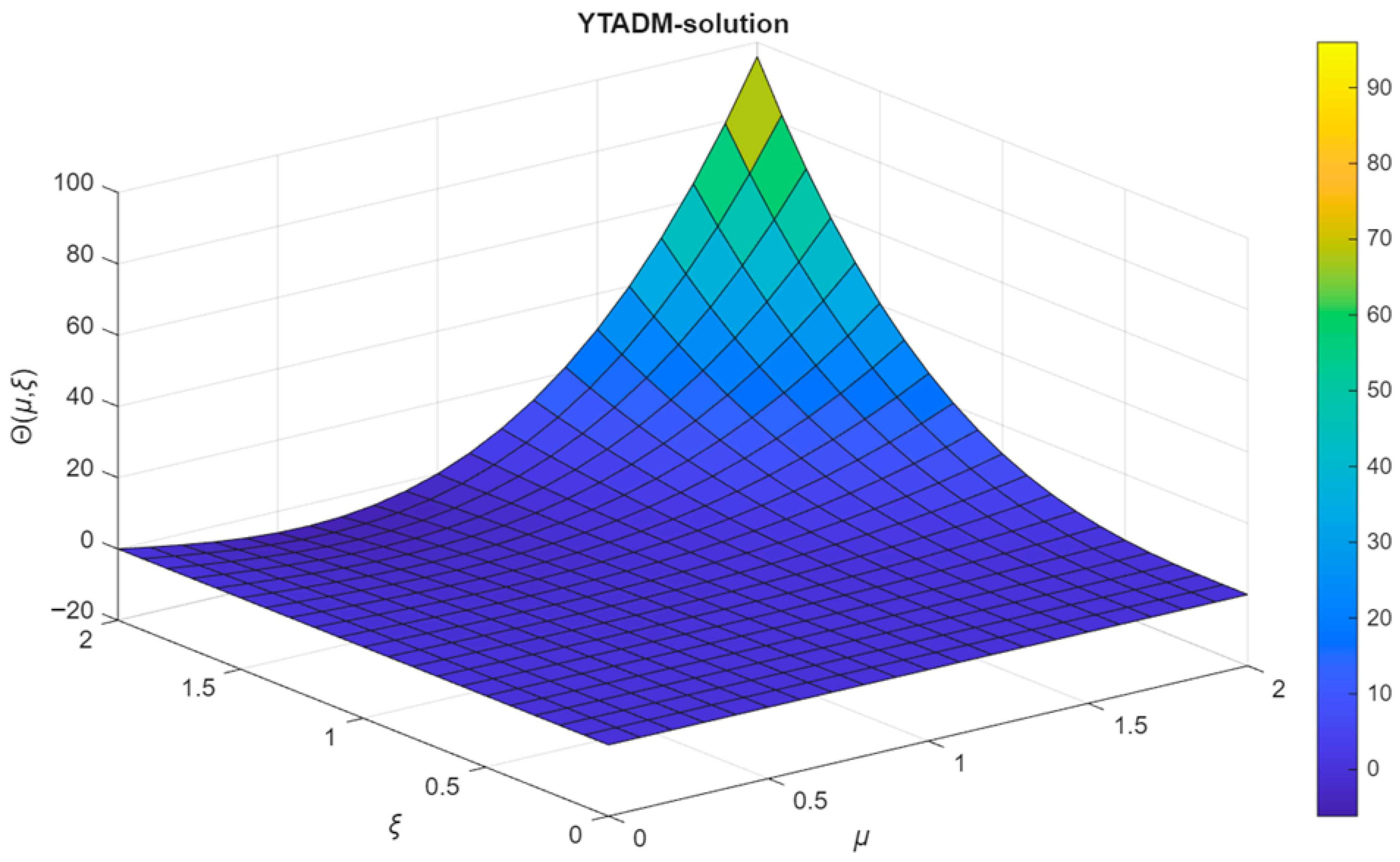
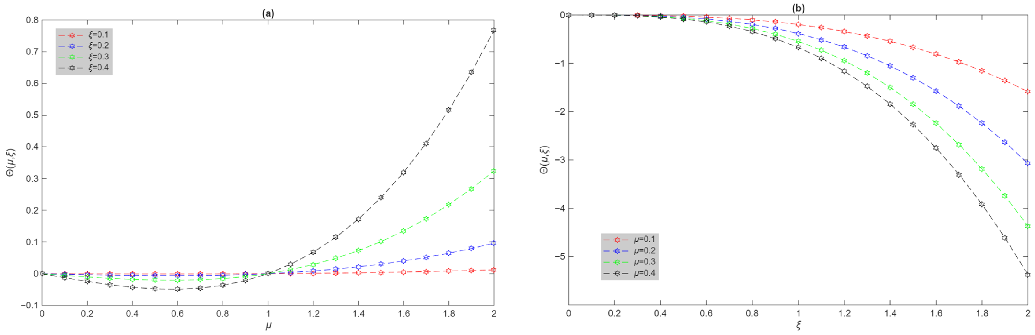
The behavior of the YTADM solution for Example 1 is illustrated in Figure 1 and Figure 2. Figure 1 presents the three-dimensional surface plot for $\eta =1$, whereas Figure 2 displays the solution profiles for different values of $\xi$ and $\mu$.

Example 2.

Consider the linear DFPDE as follows:

$$\begin{array}{cc}\hfill {}^{C}D_{\xi }^{\eta }\Theta (\mu ,\xi )& ={\displaystyle \frac{{\partial }^2\Theta (\mu ,\xi )}{\partial {\mu }^2}}+\Theta (\mu ,\xi -1)+{\mu }^3({\displaystyle \frac{\Gamma \left(\frac{11}{4}\right){\xi }^{\frac{7}{4}-\eta }}{\Gamma (\frac{11}{4}-\eta )}}-{\displaystyle \frac{\Gamma \left(\frac{9}{4}\right){\xi }^{\frac{5}{4}-\eta }}{\Gamma (\frac{9}{4}-\eta )}})-6\mu ({\xi }^{{\displaystyle \frac{7}{4}}}-{\xi }^{{\displaystyle \frac{5}{4}}})\hfill \\ & -{\mu }^2({(\xi -1)}^{{\displaystyle \frac{7}{4}}}-{(\xi -1)}^{{\displaystyle \frac{5}{4}}}),\hfill \end{array}$$

(39)

with the initial condition

$$\Theta (\mu ,0)=0,\Theta (0,\xi )=0,\Theta (1,\xi )={\xi }^{{\displaystyle \frac{7}{4}}}-{\xi }^{{\displaystyle \frac{5}{4}}},$$

(40)

and the exact solution

$$\Theta (\mu ,\xi )={\mu }^3({\xi }^{{\displaystyle \frac{7}{4}}}-{\xi }^{{\displaystyle \frac{5}{4}}}).$$

(41)

Solution 2.

Applying the Yang transform to both sides of Equation (39) gives

$$\begin{array}{cc}\hfill \mathcal{R}(\mu ,\xi )& =\chi \Theta (\mu ,0)+{\chi }^{\eta }\mathsf{Y}[{\displaystyle \frac{{\partial }^2\Theta (\mu ,\xi )}{\partial {\mu }^2}}+\Theta (\mu ,\xi -1)+{\mu }^3({\displaystyle \frac{\Gamma \left(\frac{11}{4}\right){\xi }^{\frac{7}{4}-\eta }}{\Gamma (\frac{11}{4}-\eta )}}-{\displaystyle \frac{\Gamma \left(\frac{9}{4}\right){\xi }^{\frac{5}{4}-\eta }}{\Gamma (\frac{9}{4}-\eta )}})\hfill \\ & -6\mu ({\xi }^{{\displaystyle \frac{7}{4}}}-{\xi }^{{\displaystyle \frac{5}{4}}})-{\mu }^2({(\xi -1)}^{{\displaystyle \frac{7}{4}}}-{(\xi -1)}^{{\displaystyle \frac{5}{4}}})].\hfill \end{array}$$

(42)

Applying the inverse Yang transform of Equation (42) gives

$$\begin{array}{cc}\hfill \Theta (\mu ,\xi )& =\Theta (\mu ,0)+{\mathsf{Y}}^{-1}\left[{\chi }^{\eta }\mathsf{Y}\right[{\displaystyle \frac{{\partial }^2\Theta (\mu ,\xi )}{\partial {\mu }^2}}+\Theta (\mu ,\xi -1)+{\mu }^3({\displaystyle \frac{\Gamma \left(\frac{11}{4}\right){\xi }^{\frac{7}{4}-\eta }}{\Gamma (\frac{11}{4}-\eta )}}-{\displaystyle \frac{\Gamma \left(\frac{9}{4}\right){\xi }^{\frac{5}{4}-\eta }}{\Gamma (\frac{9}{4}-\eta )}})\hfill \\ & -6\mu ({\xi }^{{\displaystyle \frac{7}{4}}}-{\xi }^{{\displaystyle \frac{5}{4}}})-{\mu }^2({(\xi -1)}^{{\displaystyle \frac{7}{4}}}-{(\xi -1)}^{{\displaystyle \frac{5}{4}}})\left]\right].\hfill \end{array}$$

(43)

Assume that

$$\Theta (\mu ,\xi )={\displaystyle \sum _{n=0}^{\infty }}{\Theta }_n.$$

(44)

Substituting Equation (44) into Equation (43), we have

$$\begin{array}{cc}\hfill {\displaystyle \sum _{n=0}^{\infty }}{\Theta }_n(\mu ,\xi )& =\Theta (\mu ,0)+{\mathsf{Y}}^{-1}\left[{\chi }^{\eta }\mathsf{Y}\right[{\displaystyle \sum _{n=0}^{\infty }}{\displaystyle \frac{{\partial }^2{\Theta }_n(\mu ,\xi )}{\partial {\mu }^2}}+{\displaystyle \sum _{n=0}^{\infty }}{\Theta }_n(\mu ,\xi -1)+{\mu }^3({\displaystyle \frac{\Gamma \left(\frac{11}{4}\right){\xi }^{\frac{7}{4}-\eta }}{\Gamma (\frac{11}{4}-\eta )}}-{\displaystyle \frac{\Gamma \left(\frac{9}{4}\right){\xi }^{\frac{5}{4}-\eta }}{\Gamma (\frac{9}{4}-\eta )}})\hfill \\ & -6\mu ({\xi }^{{\displaystyle \frac{7}{4}}}-{\xi }^{{\displaystyle \frac{5}{4}}})-{\mu }^2({(\xi -1)}^{{\displaystyle \frac{7}{4}}}-{(\xi -1)}^{{\displaystyle \frac{5}{4}}})\left]\right].\hfill \end{array}$$

(45)

Equating both sides of Equation (45), we have the following:

$$\left\{\begin{array}{c}{\Theta }_0(\mu ,\xi )={\mathsf{Y}}^{-1}\left[{\chi }^{\eta }\mathsf{Y}\right[{\mu }^3({\displaystyle \frac{\Gamma \left(\frac{11}{4}\right){\xi }^{\frac{7}{4}-\eta }}{\Gamma (\frac{11}{4}-\eta )}}-{\displaystyle \frac{\Gamma \left(\frac{9}{4}\right){\xi }^{\frac{5}{4}-\eta }}{\Gamma (\frac{9}{4}-\eta )}})\left]\right],\hfill \\ {\Theta }_1(\mu ,\xi )={\mathsf{Y}}^{-1}\left[{\chi }^{\eta }\mathsf{Y}\right[{\displaystyle \frac{{\partial }^2{\Theta }_0(\mu ,\xi )}{\partial {\mu }^2}}+{\Theta }_0(\mu ,\xi -1)-6\mu ({\xi }^{{\displaystyle \frac{7}{4}}}-{\xi }^{{\displaystyle \frac{5}{4}}})-{\mu }^2({(\xi -1)}^{{\displaystyle \frac{7}{4}}}-{(\xi -1)}^{{\displaystyle \frac{5}{4}}})\left]\right],\hfill \\ ⋮\hfill \\ {\Theta }_{n+1}(\mu ,\xi )={\mathsf{Y}}^{-1}\left[{\chi }^{\eta }\mathsf{Y}\right[{\displaystyle \frac{{\partial }^2{\Theta }_n(\mu ,\xi )}{\partial {\mu }^2}}+{\Theta }_n(\mu ,\xi -1)-6\mu ({\xi }^{{\displaystyle \frac{7}{4}}}-{\xi }^{{\displaystyle \frac{5}{4}}})-{\mu }^2({(\xi -1)}^{{\displaystyle \frac{7}{4}}}-{(\xi -1)}^{{\displaystyle \frac{5}{4}}})\left]\right],n\ge 1.\hfill \end{array}\right.$$

(46)

$$\begin{array}{cc}\hfill {\Theta }_0(\mu ,\xi )& ={\mathsf{Y}}^{-1}\left[{\chi }^{\eta }\mathsf{Y}\left[{\mu }^3({\displaystyle \frac{\Gamma \left(\frac{11}{4}\right){\xi }^{\frac{7}{4}-\eta }}{\Gamma (\frac{11}{4}-\eta )}}-{\displaystyle \frac{\Gamma \left(\frac{9}{4}\right){\xi }^{\frac{5}{4}-\eta }}{\Gamma (\frac{9}{4}-\eta )}})\right]\right]\hfill \\ \hfill & ={\mu }^3({\displaystyle \frac{\Gamma \left(\frac{11}{4}\right)}{\Gamma (\frac{11}{4}-\eta )}}-{\displaystyle \frac{\Gamma \left(\frac{9}{4}\right)}{\Gamma (\frac{9}{4}-\eta )}}){\mathsf{Y}}^{-1}\left[{\chi }^{\eta }\mathsf{Y}\left[{\xi }^{{\displaystyle \frac{7}{4}}-\eta }-{\xi }^{{\displaystyle \frac{5}{4}}-\eta }\right]\right]\hfill \\ \hfill & ={\mu }^3({\xi }^{{\displaystyle \frac{7}{4}}}-{\xi }^{{\displaystyle \frac{5}{4}}}).\hfill \end{array}$$

(47)

$$\begin{array}{cc}\hfill {\Theta }_1(\mu ,\xi )& ={\mathsf{Y}}^{-1}\left[{\chi }^{\eta }\mathsf{Y}\left[{\displaystyle \frac{{\partial }^2{\Theta }_0(\mu ,\xi )}{\partial {\mu }^2}}+{\Theta }_0(\mu ,\xi -1)-6\mu ({\xi }^{{\displaystyle \frac{7}{4}}}-{\xi }^{{\displaystyle \frac{5}{4}}})-{\mu }^2({(\xi -1)}^{{\displaystyle \frac{7}{4}}}-{(\xi -1)}^{{\displaystyle \frac{5}{4}}})\right]\right]\hfill \\ \hfill & ={\mathsf{Y}}^{-1}\left[{\chi }^{\eta }\mathsf{Y}\right[6\mu ({\xi }^{{\displaystyle \frac{7}{4}}}-{\xi }^{{\displaystyle \frac{5}{4}}})+{\mu }^2({(\xi -1)}^{{\displaystyle \frac{7}{4}}}-{(\xi -1)}^{{\displaystyle \frac{5}{4}}})-6\mu ({\xi }^{{\displaystyle \frac{7}{4}}}-{\xi }^{{\displaystyle \frac{5}{4}}})\hfill \\ & -{\mu }^2({(\xi -1)}^{{\displaystyle \frac{7}{4}}}-{(\xi -1)}^{{\displaystyle \frac{5}{4}}})\left]\right]\hfill \\ \hfill & =0.\hfill \end{array}$$

(48)

Therefore, the remaining terms of the series ${\Theta }_2={\Theta }_3,\cdots {\Theta }_n=0$. The YTADM solution is given by

$$\begin{array}{c}\hfill \Theta (\mu ,\xi )={\mu }^3({\xi }^{{\displaystyle \frac{7}{4}}}-{\xi }^{{\displaystyle \frac{5}{4}}}).\end{array}$$

(49)

For $\xi =0.2$, the obtained numerical results illustrate the performance of the proposed YTADM. The detailed comparison with the exact solution and the corresponding absolute errors is presented in

Table 2. Comparison between YTADM, exact solutions, and absolute errors, for $\xi =0.2$ of Example 2.

$\mathit{\xi }$	$\mathit{\mu }$	YTADM	Exact Sol	YTADM Error
	0.1	−0.0000739341	−0.0000739341	0
	0.2	−0.0005914729	−0.0005914729	0
	0.3	−0.0019962210	−0.0019962210	0
	0.4	−0.0047317830	−0.0047317830	0
0.2	0.5	−0.0092417637	−0.0092417637	0
	0.6	−0.0159697677	−0.0159697677	0
	0.7	−0.0253593996	−0.0253593996	0
	0.8	−0.0378542642	−0.0378542642	0
	0.9	−0.0538979660	−0.0538979660	0
	1.0	−0.0739341097	−0.0739341097	0

.

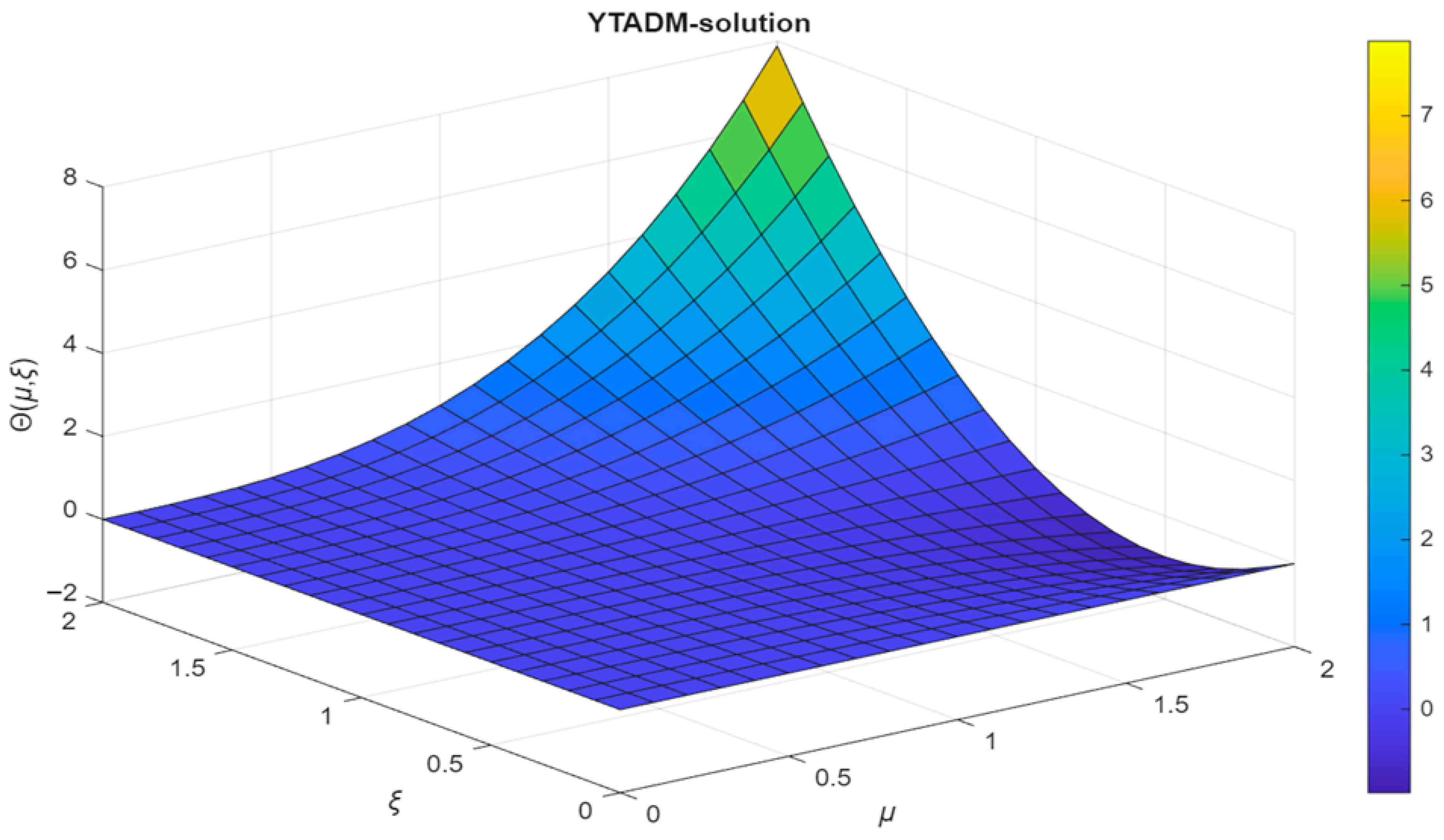
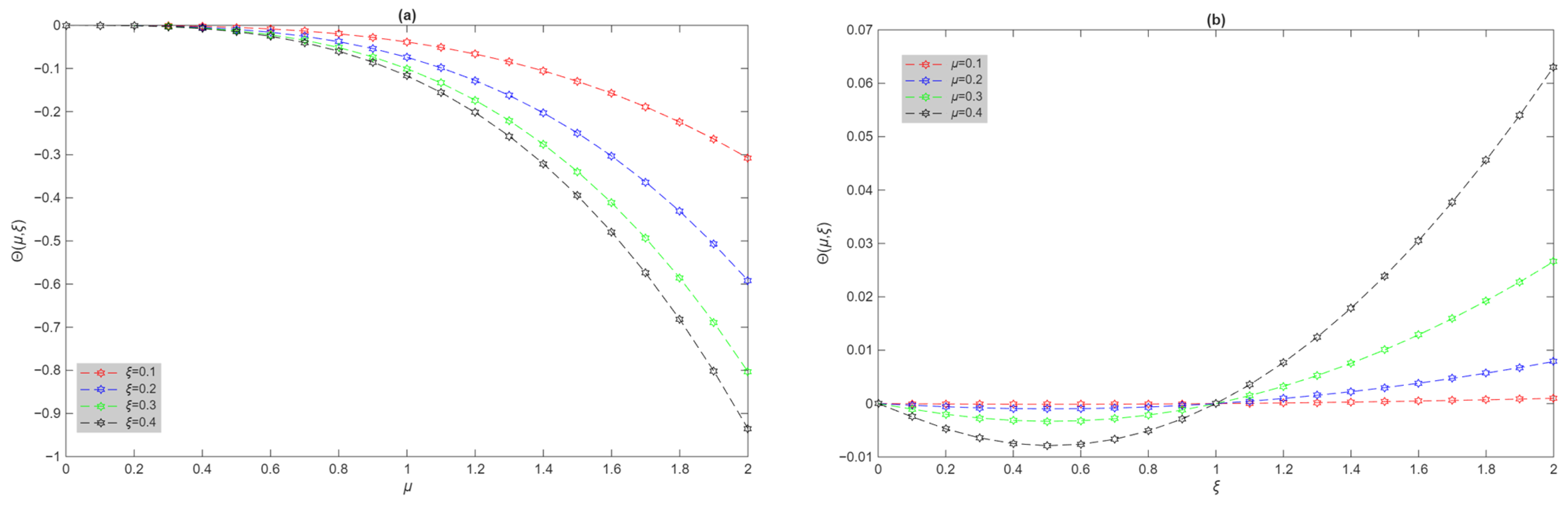
The behavior of the YTADM solution for Example 2 is illustrated in Figure 3 and Figure 4. Figure 3 presents the three-dimensional surface plot for $\eta =1$, whereas Figure 4 displays the solution profiles for different values of $\xi$ and $\mu$.

Example 3.

Consider the nonlinear proportional DFPDE for the generalized Burgers equation as follows:

$$\begin{array}{cc}\hfill {}^{C}D_{\xi }^{\eta }\Theta (\mu ,\xi )& ={\displaystyle \frac{{\partial }^2\Theta (\mu ,\xi )}{\partial {\mu }^2}}+\Theta \left({\displaystyle \frac{\mu }{2}},{\displaystyle \frac{\xi }{2}}\right){\displaystyle \frac{\partial }{\partial \mu }}\Theta \left(\mu ,{\displaystyle \frac{\xi }{2}}\right)-{\displaystyle \frac{5}{2}}\Theta (\mu ,\xi ),\hfill \end{array}$$

(50)

with the initial condition

$$\Theta (\mu ,0)=\mu ,$$

(51)

and the exact solution

$$\Theta (\mu ,\xi )=\mu e^{-2\xi }.$$

(52)

Solution 3.

Applying the Yang transform to both sides of Equation (50) gives

$$\begin{array}{c}\hfill \mathcal{R}(\mu ,\xi )=\chi \Theta (\mu ,0)+{\chi }^{\eta }\mathsf{Y}\left[{\displaystyle \frac{{\partial }^2\Theta (\mu ,\xi )}{\partial {\mu }^2}}+\Theta \left({\displaystyle \frac{\mu }{2}},{\displaystyle \frac{\xi }{2}}\right){\displaystyle \frac{\partial }{\partial \mu }}\Theta \left(\mu ,{\displaystyle \frac{\xi }{2}}\right)-{\displaystyle \frac{5}{2}}\Theta (\mu ,\xi )\right].\end{array}$$

(53)

Applying the inverse Yang transform to Equation (53) gives

$$\begin{array}{cc}\hfill \Theta (\mu ,\xi )& =\Theta (\mu ,0)+{\mathsf{Y}}^{-1}\left[{\chi }^{\eta }\mathsf{Y}\left[{\displaystyle \frac{{\partial }^2\Theta (\mu ,\xi )}{\partial {\mu }^2}}+\Theta \left({\displaystyle \frac{\mu }{2}},{\displaystyle \frac{\xi }{2}}\right){\displaystyle \frac{\partial }{\partial \mu }}\Theta \left(\mu ,{\displaystyle \frac{\xi }{2}}\right)-{\displaystyle \frac{5}{2}}\Theta (\mu ,\xi )\right]\right].\hfill \end{array}$$

(54)

Assume that

$$\Theta (\mu ,\xi )={\displaystyle \sum _{n=0}^{\infty }}{\Theta }_n,\Theta \left({\displaystyle \frac{\mu }{2}},{\displaystyle \frac{\xi }{2}}\right){\displaystyle \frac{\partial }{\partial \mu }}\Theta \left(\mu ,{\displaystyle \frac{\xi }{2}}\right)={\displaystyle \sum _{n=0}^{\infty }}{\mathcal{A}}_n,$$

(55)

where ${\mathcal{A}}_n$ is defined by

$$\begin{array}{cc}\hfill {\mathcal{A}}_0& ={\Theta }_0\left({\displaystyle \frac{\mu }{2}},{\displaystyle \frac{\xi }{2}}\right){\displaystyle \frac{\partial }{\partial \mu }}{\Theta }_0\left(\mu ,{\displaystyle \frac{\xi }{2}}\right)\hfill \\ \hfill {\mathcal{A}}_1& ={\Theta }_0\left({\displaystyle \frac{\mu }{2}},{\displaystyle \frac{\xi }{2}}\right){\displaystyle \frac{\partial }{\partial \mu }}{\Theta }_1\left(\mu ,{\displaystyle \frac{\xi }{2}}\right)+{\Theta }_1\left({\displaystyle \frac{\mu }{2}},{\displaystyle \frac{\xi }{2}}\right){\displaystyle \frac{\partial }{\partial \mu }}{\Theta }_0\left(\mu ,{\displaystyle \frac{\xi }{2}}\right)\hfill \\ \hfill {\mathcal{A}}_2& ={\Theta }_0\left({\displaystyle \frac{\mu }{2}},{\displaystyle \frac{\xi }{2}}\right){\displaystyle \frac{\partial }{\partial \mu }}{\Theta }_2\left(\mu ,{\displaystyle \frac{\xi }{2}}\right)+{\Theta }_1\left({\displaystyle \frac{\mu }{2}},{\displaystyle \frac{\xi }{2}}\right){\displaystyle \frac{\partial }{\partial \mu }}{\Theta }_1\left(\mu ,{\displaystyle \frac{\xi }{2}}\right)+{\Theta }_2\left({\displaystyle \frac{\mu }{2}},{\displaystyle \frac{\xi }{2}}\right){\displaystyle \frac{\partial }{\partial \mu }}{\Theta }_0\left(\mu ,{\displaystyle \frac{\xi }{2}}\right).\hfill \\ \hfill ⋮& \hfill \end{array}$$

Substituting Equation (55) into (54), we obtain

$$\begin{array}{cc}\hfill {\displaystyle \sum _{n=0}^{\infty }}{\Theta }_n(\mu ,\xi )& =\Theta (\mu ,0)+{\mathsf{Y}}^{-1}\left[{\chi }^{\eta }\mathsf{Y}\left[{\displaystyle \sum _{n=0}^{\infty }}{\displaystyle \frac{{\partial }^2{\Theta }_n(\mu ,\xi )}{\partial {\mu }^2}}+{\displaystyle \sum _{n=0}^{\infty }}{\mathcal{A}}_n-{\displaystyle \frac{5}{2}}{\displaystyle \sum _{n=0}^{\infty }}{\Theta }_n\right]\right].\hfill \end{array}$$

(56)

Equating both sides of Equation (56), we have the following:

$$\left\{\begin{array}{c}{\Theta }_0(\mu ,\xi )=\mu ,\hfill \\ {\Theta }_1(\mu ,\xi )={\mathsf{Y}}^{-1}\left[{\chi }^{\eta }\mathsf{Y}\left[{\displaystyle \frac{{\partial }^2{\Theta }_0(\mu ,\xi )}{\partial {\mu }^2}}+{\mathcal{A}}_0-{\displaystyle \frac{5}{2}}{\Theta }_0(\mu ,\xi )\right]\right],\hfill \\ ⋮\hfill \\ {\Theta }_{n+1}(\mu ,\xi )={\mathsf{Y}}^{-1}\left[{\chi }^{\eta }\mathsf{Y}\left[{\displaystyle \frac{{\partial }^2{\Theta }_n(\mu ,\xi )}{\partial {\mu }^2}}+{\mathcal{A}}_n-{\displaystyle \frac{5}{2}}{\Theta }_n(\mu ,\xi )\right]\right],n\ge 1.\hfill \end{array}\right.$$

$$\begin{array}{cc}\hfill {\Theta }_1(\mu ,\xi )& ={\mathsf{Y}}^{-1}\left[{\chi }^{\eta }\mathsf{Y}\left[{\displaystyle \frac{{\partial }^2{\Theta }_0(\mu ,\xi )}{\partial {\mu }^2}}+{\mathcal{A}}_0-{\displaystyle \frac{5}{2}}{\Theta }_0(\mu ,\xi )\right]\right]\hfill \\ \hfill & ={\mathsf{Y}}^{-1}\left[{\chi }^{\eta }\mathsf{Y}\left[{\displaystyle \frac{\mu }{2}}-{\displaystyle \frac{5\mu }{2}}\right]\right]=-{\displaystyle \frac{2\mu {\xi }^{\eta }}{\Gamma (\eta +1)}}.\hfill \end{array}$$

(57)

$$\begin{array}{cc}\hfill {\Theta }_2(\mu ,\xi )& ={\mathsf{Y}}^{-1}\left[{\chi }^{\eta }\mathsf{Y}\left[{\displaystyle \frac{{\partial }^2{\Theta }_1(\mu ,\xi )}{\partial {\mu }^2}}+{\mathcal{A}}_1-{\displaystyle \frac{5}{2}}{\Theta }_1(\mu ,\xi )\right]\right]\hfill \\ \hfill & ={\mathsf{Y}}^{-1}\left[{\chi }^{\eta }\mathsf{Y}\left[-{\displaystyle \frac{2\mu {\xi }^{\eta }}{2^{\eta }\Gamma (\eta +1)}}+{\displaystyle \frac{5\mu {\xi }^{\eta }}{\Gamma (\eta +1)}}\right]\right]=-{\displaystyle \frac{2\mu {\xi }^{2\eta }}{2^{\eta }\Gamma (2\eta +1)}}+{\displaystyle \frac{5\mu {\xi }^{2\eta }}{\Gamma (2\eta +1)}}\hfill \\ \hfill & ={\displaystyle \frac{\mu {\xi }^{2\eta }}{\Gamma (2\eta +1)}}\left(5-{\displaystyle \frac{2}{2^{\eta }}}\right).\hfill \end{array}$$

(58)

$$\begin{array}{cc}\hfill {\Theta }_3(\mu ,\xi )& ={\mathsf{Y}}^{-1}\left[{\chi }^{\eta }\mathsf{Y}\left[{\displaystyle \frac{{\partial }^2{\Theta }_2(\mu ,\xi )}{\partial {\mu }^2}}+{\mathcal{A}}_2-{\displaystyle \frac{5}{2}}{\Theta }_2(\mu ,\xi )\right]\right]\hfill \\ \hfill & ={\mathsf{Y}}^{-1}\left[{\chi }^{\eta }\mathsf{Y}\left[{\displaystyle \frac{\mu {\xi }^{2\eta }}{2^{2\eta }\Gamma (2\eta +1)}}\left(5-{\displaystyle \frac{2}{2^{\eta }}}\right)+{\displaystyle \frac{2\mu {\xi }^{2\eta }}{2^{2\eta }\Gamma {(\eta +1)}^2}}-{\displaystyle \frac{5}{2}}\left[{\displaystyle \frac{\mu {\xi }^{2\eta }}{\Gamma (2\eta +1)}}\left(5-{\displaystyle \frac{2}{2^{\eta }}}\right)\right]\right]\right]\hfill \\ \hfill & ={\mathsf{Y}}^{-1}\left[{\chi }^{\eta }\mathsf{Y}\left({\displaystyle \frac{\mu {\xi }^{2\eta }}{\Gamma (2\eta +1)}}\left[\left(5-{\displaystyle \frac{2}{2^{\eta }}}\right)\left({\displaystyle \frac{1}{2^{2\eta }}}-{\displaystyle \frac{5}{2}}\right)\right]+{\displaystyle \frac{2\mu {\xi }^{2\eta }}{2^{2\eta }\Gamma {(\eta +1)}^2}}\right)\right]\hfill \\ \hfill & =\left(5-{\displaystyle \frac{2}{2^{\eta }}}\right)\left({\displaystyle \frac{1}{2^{2\eta }}}-{\displaystyle \frac{5}{2}}\right){\displaystyle \frac{\mu {\xi }^{3\eta }}{\Gamma (3\eta +1)}}+{\displaystyle \frac{2\Gamma (2\eta +1)\mu {\xi }^{3\eta }}{2^{2\eta }\Gamma {(\eta +1)}^2\Gamma (3\eta +1)}}.\hfill \end{array}$$

(59)

Therefore, the YTADM solution is given by

$$\begin{array}{cc}\hfill \Theta (\mu ,\xi )& =\mu -{\displaystyle \frac{2\mu {\xi }^{\eta }}{\Gamma (\eta +1)}}+{\displaystyle \frac{\mu {\xi }^{2\eta }}{\Gamma (2\eta +1)}}\left(5-{\displaystyle \frac{2}{2^{\eta }}}\right)+\left(5-{\displaystyle \frac{2}{2^{\eta }}}\right)\left({\displaystyle \frac{1}{2^{2\eta }}}-{\displaystyle \frac{5}{2}}\right){\displaystyle \frac{\mu {\xi }^{3\eta }}{\Gamma (3\eta +1)}}\hfill \\ \hfill & +{\displaystyle \frac{2\Gamma (2\eta +1)\mu {\xi }^{3\eta }}{2^{2\eta }\Gamma {(\eta +1)}^2\Gamma (3\eta +1)}}+\cdots \hfill \end{array}$$

(60)

and when $\eta =1$, the YTADM solution is reduced to

$$\begin{array}{c}\hfill \Theta (\mu ,\xi )=\mu \left(1-2\xi +2{\xi }^2-{\displaystyle \frac{4}{3}}{\xi }^3+\dots \right)=\mu e^{-2\xi }.\end{array}$$

(61)

For the convergence analysis, we consider the case $\mu =0.3$, $\xi =0.3$ and $\eta =1$.

$$\begin{array}{cc}\hfill r_0& ={\displaystyle \frac{\parallel {\Theta }_1\parallel }{\parallel {\Theta }_0\parallel }}={\displaystyle \frac{\parallel -0.180000\parallel }{\parallel 0.300000\parallel }}=0.600000<1,\hfill \\ \hfill r_1& ={\displaystyle \frac{\parallel {\Theta }_2\parallel }{\parallel {\Theta }_1\parallel }}={\displaystyle \frac{\parallel 0.054000\parallel }{\parallel -0.180000\parallel }}=0.300000<1,\hfill \\ \hfill r_2& ={\displaystyle \frac{\parallel {\Theta }_3\parallel }{\parallel {\Theta }_2\parallel }}={\displaystyle \frac{\parallel -0.010800\parallel }{\parallel 0.054000\parallel }}=0.200000<1.\hfill \\ \hfill ⋮& \end{array}$$

Remark 3.

The above ratios are computed for the representative values $\mu =0.3$, $\xi =0.3$, and $\eta =1$. For $\eta =1$, the condition $r_n<1$ is satisfied for $0<\xi <0.5$, indicating that the numerical ratio test depends on the selected parameter values.

For $\mu =0.2$, the YTADM solutions are computed for different values of the fractional order $\eta$. The corresponding numerical results are presented in

Table 3. YTADM solutions, exact solutions, and absolute errors for $\mu =0.2$ of Example 3.

$\mathit{\mu }$	$\mathit{\xi }$	$\mathit{\eta }=0.7$	$\mathit{\eta }=0.8$	$\mathit{\eta }=0.9$	$\mathit{\eta }=1$
	0.1	0.13136804	0.14352571	0.15433618	0.16373333
	0.2	0.09982342	0.11226749	0.12340060	0.13386667
	0.3	0.07317899	0.08745026	0.09870813	0.10880000
	0.4	0.04538520	0.06393709	0.07682338	0.08693333
	0.5	0.01346044	0.03865543	0.05523431	0.06666667
0.2	0.6	$-0.02443712$	0.00939415	0.03185180	0.04640000
	0.7	$-0.06958699$	$-0.02559005$	0.00483483	0.02453333
	0.8	$-0.12294506$	$-0.06774779$	$-0.02749158$	$-0.00053333$
	0.9	$-0.18526175$	$-0.11832938$	$-0.06668193$	$-0.03040000$
	1.0	$-0.25714776$	$-0.17843937$	$-0.11419826$	$-0.06666667$

, while the comparison with the exact solutions and the corresponding absolute errors is given in

Table 4. Comparison between exact solutions and absolute errors of Example 3.

$\mathit{\mu }$	$\mathit{\xi }$	Exact Sol	Absolute Error	CPU Time
	0.1	0.16374615	$1.28173\times {10}^{-5}$	0.00016771
	0.2	0.13406401	$1.97343\times {10}^{-4}$	0.00008225
	0.3	0.10976233	$9.62327\times {10}^{-4}$	0.00007867
	0.4	0.08986579	$2.93246\times {10}^{-3}$	0.00007783
0.2	0.5	0.07357589	$6.90922\times {10}^{-3}$	0.00007721
	0.6	0.06023884	$1.38388\times {10}^{-2}$	0.00007750
	0.7	0.04931939	$2.47861\times {10}^{-2}$	0.00007737
	0.8	0.04037930	$4.09126\times {10}^{-2}$	0.00007713
	0.9	0.03305978	$6.34598\times {10}^{-2}$	0.00007696
	1.0	0.02701490	$9.36816\times {10}^{-2}$	0.00007717

.

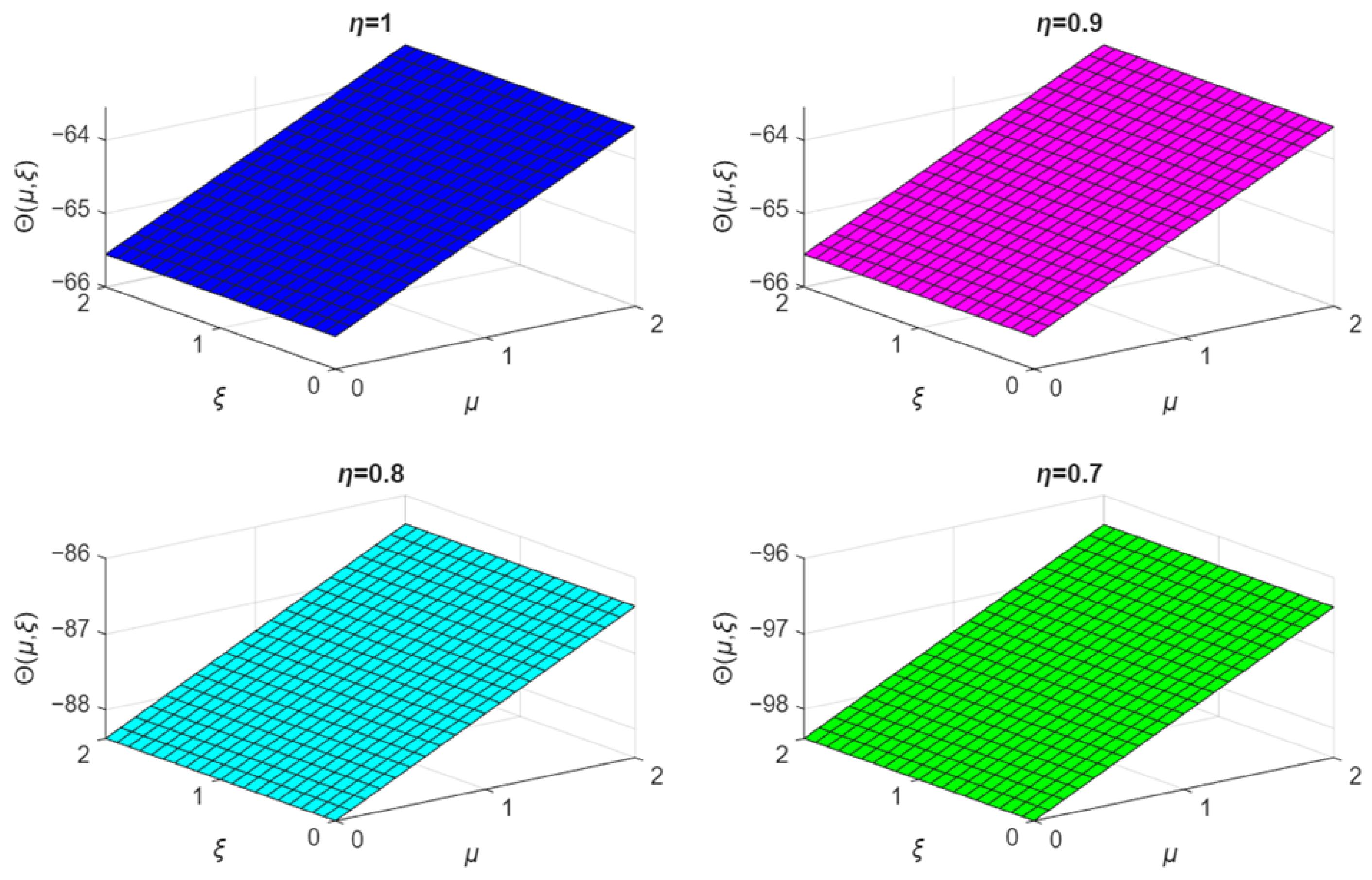
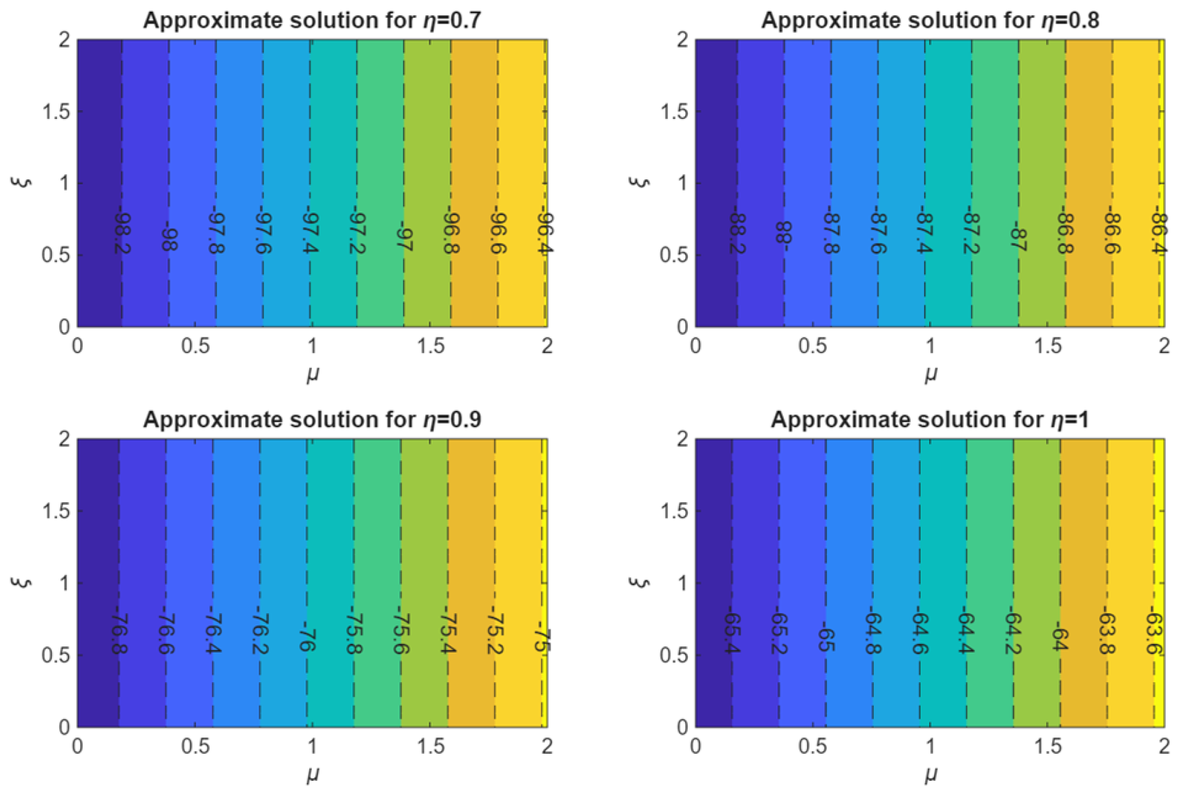
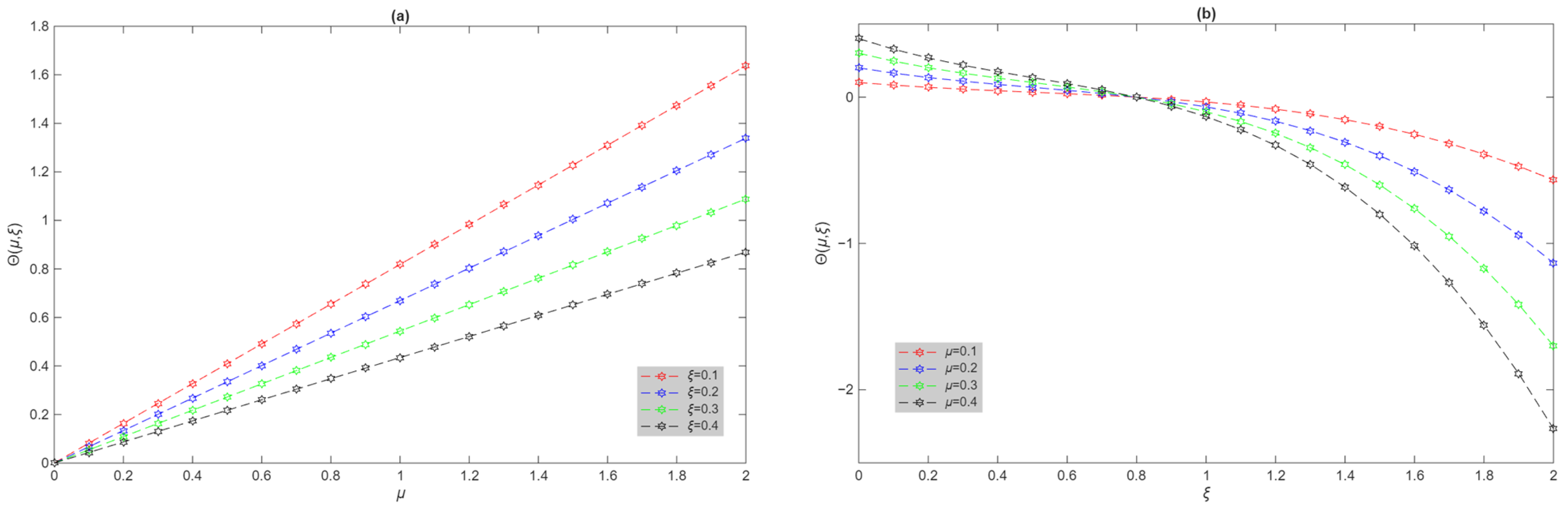
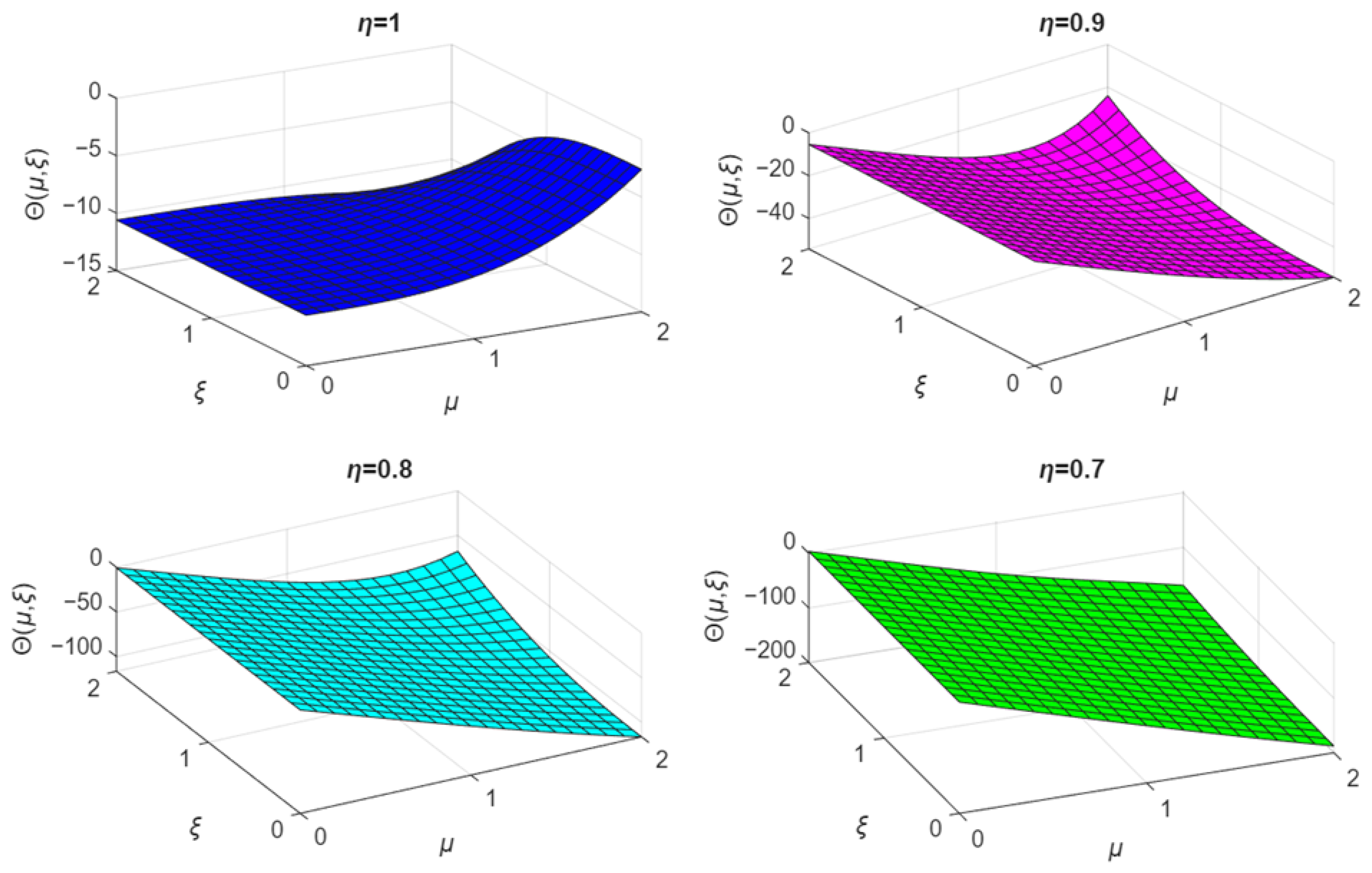
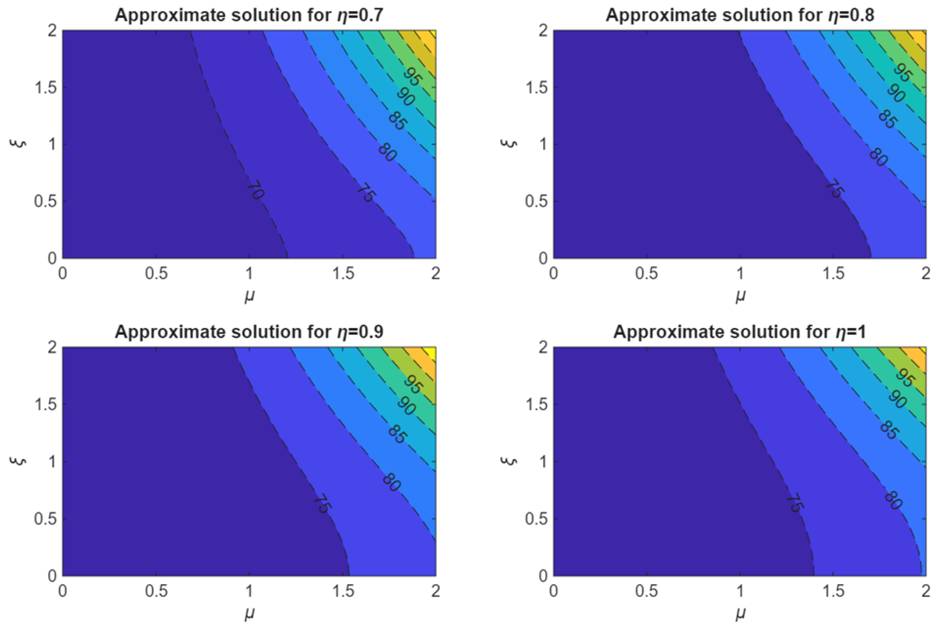
The graphical results for Example 3 are presented in Figure 5, Figure 6 and Figure 7. Figure 5 presents the three-dimensional surface plots of the YTADM solution for different fractional orders $\eta$, Figure 6 shows the corresponding contour plots, whereas Figure 7 illustrates the variation of the solution with respect to different values of $\xi$ and $\mu$.

Example 4.

Consider the nonlinear proportional DFPDE for the generalized Burgers equation as follows:

$$\begin{array}{cc}\hfill {}^{C}D_{\xi }^{\eta }\Theta (\mu ,\xi )& =\Theta \left(\mu ,{\displaystyle \frac{\xi }{2}}\right){\displaystyle \frac{{\partial }^2}{\partial {\mu }^2}}\Theta \left(\mu ,{\displaystyle \frac{\xi }{2}}\right)-(6\mu +1)\Theta (\mu ,\xi ),\hfill \end{array}$$

(62)

with the initial condition

$$\begin{array}{c}\hfill \Theta (\mu ,0)={\mu }^3,\end{array}$$

(63)

and the exact solution

$$\begin{array}{c}\hfill \Theta (\mu ,\xi )={\mu }^3{e}^{-\xi }.\end{array}$$

(64)

Solution 4.

Applying the Yang transform to both sides of Equation (62) gives

$$\begin{array}{cc}\hfill \mathcal{R}(\mu ,\xi )& =\chi \Theta (\mu ,0)+{\chi }^{\eta }\mathsf{Y}\left[\Theta \left(\mu ,{\displaystyle \frac{\xi }{2}}\right){\displaystyle \frac{{\partial }^2}{\partial {\mu }^2}}\Theta \left(\mu ,{\displaystyle \frac{\xi }{2}}\right)-(6\mu +1)\Theta (\mu ,\xi )\right].\hfill \end{array}$$

(65)

Applying the inverse Yang transform of Equation (65) gives

$$\begin{array}{cc}\hfill \Theta (\mu ,\xi )& =\Theta (\mu ,0)+{\mathsf{Y}}^{-1}\left[{\chi }^{\eta }\mathsf{Y}\left[\Theta \left(\mu ,{\displaystyle \frac{\xi }{2}}\right){\displaystyle \frac{{\partial }^2}{\partial {\mu }^2}}\Theta \left(\mu ,{\displaystyle \frac{\xi }{2}}\right)-(6\mu +1)\Theta (\mu ,\xi )\right]\right].\hfill \end{array}$$

(66)

Assume that

$$\Theta (\mu ,\xi )={\displaystyle \sum _{n=0}^{\infty }}{\Theta }_n,\Theta \left(\mu ,{\displaystyle \frac{\xi }{2}}\right){\displaystyle \frac{{\partial }^2}{\partial {\mu }^2}}\Theta \left(\mu ,{\displaystyle \frac{\xi }{2}}\right)={\displaystyle \sum _{n=0}^{\infty }}{\mathcal{B}}_n,$$

(67)

where ${\mathcal{B}}_n$ is defined by

$$\begin{array}{cc}\hfill {\mathcal{B}}_0& ={\Theta }_0\left(\mu ,{\displaystyle \frac{\xi }{2}}\right){\displaystyle \frac{{\partial }^2}{\partial {\mu }^2}}{\Theta }_0\left(\mu ,{\displaystyle \frac{\xi }{2}}\right)\hfill \\ \hfill {\mathcal{B}}_1& ={\Theta }_0\left(\mu ,{\displaystyle \frac{\xi }{2}}\right){\displaystyle \frac{{\partial }^2}{\partial {\mu }^2}}{\Theta }_1\left(\mu ,{\displaystyle \frac{\xi }{2}}\right)+{\Theta }_1\left(\mu ,{\displaystyle \frac{\xi }{2}}\right){\displaystyle \frac{{\partial }^2}{\partial {\mu }^2}}{\Theta }_0\left(\mu ,{\displaystyle \frac{\xi }{2}}\right)\hfill \\ \hfill {\mathcal{B}}_2& ={\Theta }_0\left(\mu ,{\displaystyle \frac{\xi }{2}}\right){\displaystyle \frac{{\partial }^2}{\partial {\mu }^2}}{\Theta }_2\left(\mu ,{\displaystyle \frac{\xi }{2}}\right)+{\Theta }_1\left(\mu ,{\displaystyle \frac{\xi }{2}}\right){\displaystyle \frac{{\partial }^2}{\partial {\mu }^2}}{\Theta }_1\left(\mu ,{\displaystyle \frac{\xi }{2}}\right)+{\Theta }_2\left(\mu ,{\displaystyle \frac{\xi }{2}}\right){\displaystyle \frac{{\partial }^2}{\partial {\mu }^2}}{\Theta }_0\left(\mu ,{\displaystyle \frac{\xi }{2}}\right).\hfill \\ \hfill ⋮& \hfill \end{array}$$

Substituting Equation (67) into Equation (66), we obtain

$$\begin{array}{cc}\hfill {\displaystyle \sum _{n=0}^{\infty }}{\Theta }_n(\mu ,\xi )& =\Theta (\mu ,0)+{\mathsf{Y}}^{-1}\left[{\chi }^{\eta }\mathsf{Y}\left[{\displaystyle \sum _{n=0}^{\infty }}{\mathcal{B}}_n-(6\mu +1){\displaystyle \sum _{n=0}^{\infty }}{\Theta }_n\right]\right].\hfill \end{array}$$

(68)

Equating both sides of Equation (68), we have the following:

$$\left\{\begin{array}{c}{\Theta }_0(\mu ,\xi )={\mu }^3,\hfill \\ {\Theta }_1(\mu ,\xi )={\mathsf{Y}}^{-1}\left[{\chi }^{\eta }\mathsf{Y}\left[{\mathcal{B}}_0-(6\mu +1){\Theta }_0(\mu ,\xi )\right]\right],\hfill \\ ⋮\hfill \\ {\Theta }_{n+1}(\mu ,\xi )={\mathsf{Y}}^{-1}\left[{\chi }^{\eta }\mathsf{Y}\left[{\mathcal{B}}_n-(6\mu +1){\Theta }_n(\mu ,\xi )\right]\right],n\ge 1.\hfill \end{array}\right.$$

(69)

$$\begin{array}{cc}\hfill {\Theta }_1(\mu ,\xi )& ={\mathsf{Y}}^{-1}\left[{\chi }^{\eta }\mathsf{Y}\left[{\mathcal{B}}_0-(6\mu +1){\Theta }_0(\mu ,\xi )\right]\right]\hfill \\ \hfill & ={\mathsf{Y}}^{-1}\left[{\chi }^{\eta }\mathsf{Y}\left(6{\mu }^4-(6\mu +1){\mu }^3\right)\right]\hfill \\ & =-{\displaystyle \frac{{\mu }^3{\xi }^{\eta }}{\Gamma (\eta +1)}}.\hfill \end{array}$$

(70)

$$\begin{array}{cc}\hfill {\Theta }_2(\mu ,\xi )& ={\mathsf{Y}}^{-1}\left[{\chi }^{\eta }\mathsf{Y}\left[{\mathcal{B}}_1-(6\mu +1){\Theta }_1(\mu ,\xi )\right]\right]\hfill \\ \hfill & ={\mathsf{Y}}^{-1}\left[{\chi }^{\eta }\mathsf{Y}\left[{\displaystyle \frac{-12{\mu }^4{\xi }^{\eta }}{2^{\eta }\Gamma (\eta +1)}}+(6\mu +1){\displaystyle \frac{{\mu }^3{\xi }^{\eta }}{\Gamma (\eta +1)}}\right]\right]\hfill \\ \hfill & ={\mathsf{Y}}^{-1}\left[{\chi }^{\eta }\mathsf{Y}\left[{\displaystyle \frac{{\mu }^3{\xi }^{\eta }}{\Gamma (\eta +1)}}\left[6\mu \left(1-{\displaystyle \frac{2}{2^{\eta }}}\right)+1\right]\right]\right]\hfill \\ \hfill & ={\displaystyle \frac{{\mu }^3{\xi }^{2\eta }}{\Gamma (2\eta +1)}}\left[6\mu \left(1-{\displaystyle \frac{2}{2^{\eta }}}\right)+1\right].\hfill \end{array}$$

(71)

$$\begin{array}{cc}\hfill {\Theta }_3(\mu ,\xi )& ={\mathsf{Y}}^{-1}\left[{\chi }^{\eta }\mathsf{Y}\left[{\mathcal{B}}_2-(6\mu +1){\Theta }_2(\mu ,\xi )\right]\right]\hfill \\ \hfill & ={\mathsf{Y}}^{-1}\left[{\chi }^{\eta }\mathsf{Y}\right[{\displaystyle \frac{108{\mu }^5\left(1-\frac{2}{2^{\eta }}\right)+12{\mu }^4}{2^{2\eta }\Gamma (2\eta +1)}}{\xi }^{2\eta }+{\displaystyle \frac{6{\mu }^4}{2^{2\eta }\Gamma {(\eta +1)}^2}}{\xi }^{2\eta }\hfill \\ & -{\displaystyle \frac{{\xi }^{2\eta }}{\Gamma (2\eta +1)}}\left[36{\mu }^5\left(1-{\displaystyle \frac{2}{2^{\eta }}}\right)+6{\mu }^4\left(2-{\displaystyle \frac{2}{2^{\eta }}}\right)+{\mu }^3\right]\left]\right]\hfill \\ & ={\displaystyle \frac{108{\mu }^5\left(1-\frac{2}{2^{\eta }}\right)+12{\mu }^4}{2^{2\eta }\Gamma (3\eta +1)}}{\xi }^{3\eta }+{\displaystyle \frac{6{\mu }^4\Gamma (2\eta +1)}{2^{2\eta }\Gamma {(\eta +1)}^2\Gamma (3\eta +1)}}{\xi }^{3\eta }\hfill \\ & -{\displaystyle \frac{{\xi }^{3\eta }}{\Gamma (3\eta +1)}}\left[36{\mu }^5\left(1-{\displaystyle \frac{2}{2^{\eta }}}\right)+6{\mu }^4\left(2-{\displaystyle \frac{2}{2^{\eta }}}\right)+{\mu }^3\right].\hfill \end{array}$$

(72)

Therefore, the YTADM solution is given by

$$\begin{array}{cc}\hfill \Theta (\mu ,\xi )& ={\mu }^3-{\displaystyle \frac{{\mu }^3{\xi }^{\eta }}{\Gamma (\eta +1)}}+{\displaystyle \frac{{\mu }^3{\xi }^{2\eta }}{\Gamma (2\eta +1)}}\left[6\mu \left(1-{\displaystyle \frac{2}{2^{\eta }}}\right)+1\right]\hfill \\ \hfill & +{\displaystyle \frac{108{\mu }^5\left(1-\frac{2}{2^{\eta }}\right)+12{\mu }^4}{2^{2\eta }\Gamma (3\eta +1)}}{\xi }^{3\eta }+{\displaystyle \frac{6{\mu }^4\Gamma (2\eta +1)}{2^{2\eta }\Gamma {(\eta +1)}^2\Gamma (3\eta +1)}}{\xi }^{3\eta }\hfill \\ & -{\displaystyle \frac{{\xi }^{3\eta }}{\Gamma (3\eta +1)}}\left[36{\mu }^5\left(1-{\displaystyle \frac{2}{2^{\eta }}}\right)+6{\mu }^4\left(2-{\displaystyle \frac{2}{2^{\eta }}}\right)+{\mu }^3\right]+\cdots \hfill \end{array}$$

(73)

and when $\eta =1$, the YTADM solution is reduced to

$$\begin{array}{c}\hfill \Theta (\mu ,\xi )={\mu }^3\left(1-\xi +{\displaystyle \frac{{\xi }^2}{2!}}-{\displaystyle \frac{{\xi }^3}{3!}}+\dots \right)={\mu }^3{e}^{-\xi }.\end{array}$$

(74)

For the convergence analysis, we consider the case $\mu =0.3$, $\xi =0.3$ and $\eta =1$.

$$\begin{array}{cc}\hfill r_0& ={\displaystyle \frac{\parallel {\Theta }_1\parallel }{\parallel {\Theta }_0\parallel }}={\displaystyle \frac{\parallel -0.008100\parallel }{\parallel 0.027000\parallel }}=0.300000<1,\hfill \\ \hfill r_1& ={\displaystyle \frac{\parallel {\Theta }_2\parallel }{\parallel {\Theta }_1\parallel }}={\displaystyle \frac{\parallel 0.001215\parallel }{\parallel -0.008100\parallel }}=0.150000<1,\hfill \\ \hfill r_2& ={\displaystyle \frac{\parallel {\Theta }_3\parallel }{\parallel {\Theta }_2\parallel }}={\displaystyle \frac{\parallel -0.000122\parallel }{\parallel 0.001215\parallel }}=0.100000<1.\hfill \\ \hfill ⋮& \end{array}$$

Remark 4.

The above ratios are computed for the values $\mu =0.3$, $\xi =0.3$, and $\eta =1$. For $\eta =1$, the condition $r_n<1$ is satisfied for $0<\xi \le 0.8$.

For $\mu =0.2$, the YTADM solutions are computed for different values of the fractional order $\eta$. The corresponding numerical results are presented in

Table 5. YTADM solutions for various values $\eta =0.7, 0.8, 0.9, 1$ of Example 4.

$\mathit{\mu }$	$\mathit{\xi }$	$\mathit{\eta }=0.7$	$\mathit{\eta }=0.8$	$\mathit{\eta }=0.9$	$\mathit{\eta }=1$
	0.1	0.00641774	0.00674801	0.00701893	0.00723867
	0.2	0.00558874	0.00594743	0.00626703	0.00654933
	0.3	0.00496337	0.00530553	0.00562625	0.00592400
	0.4	0.00445530	0.00476326	0.00506461	0.00535467
0.2	0.5	0.00402571	0.00429079	0.00456286	0.00483333
	0.6	0.00365236	0.00386925	0.00410692	0.00435200
	0.7	0.00332074	0.00348518	0.00368542	0.00390267
	0.8	0.00302062	0.00312830	0.00328863	0.00347733
	0.9	0.00274433	0.00279030	0.00290797	0.00306800
	1.0	0.00248594	0.00246429	0.00253563	0.00266667

, while the comparison with the exact solutions and the corresponding absolute errors is given in

Table 6. Comparison between exact solutions and absolute errors of Example 4.

$\mathit{\mu }$	$\mathit{\xi }$	Exact Sol	Absolute Error	CPU Time
	0.1	0.00723870	$3.26776\times {10}^{-8}$	0.00029058
	0.2	0.00654985	$5.12691\times {10}^{-7}$	0.00011267
	0.3	0.00592655	$2.54577\times {10}^{-6}$	0.00008917
	0.4	0.00536256	$7.89370\times {10}^{-6}$	0.00008646
0.2	0.5	0.00485225	$1.89119\times {10}^{-5}$	0.00018087
	0.6	0.00439049	$3.84931\times {10}^{-5}$	0.00009292
	0.7	0.00397268	$7.00158\times {10}^{-5}$	0.00008671
	0.8	0.00359463	$1.17298\times {10}^{-4}$	0.00008567
	0.9	0.00325256	$1.84557\times {10}^{-4}$	0.00008433
	1.0	0.00294304	$2.76369\times {10}^{-4}$	0.00008458

.

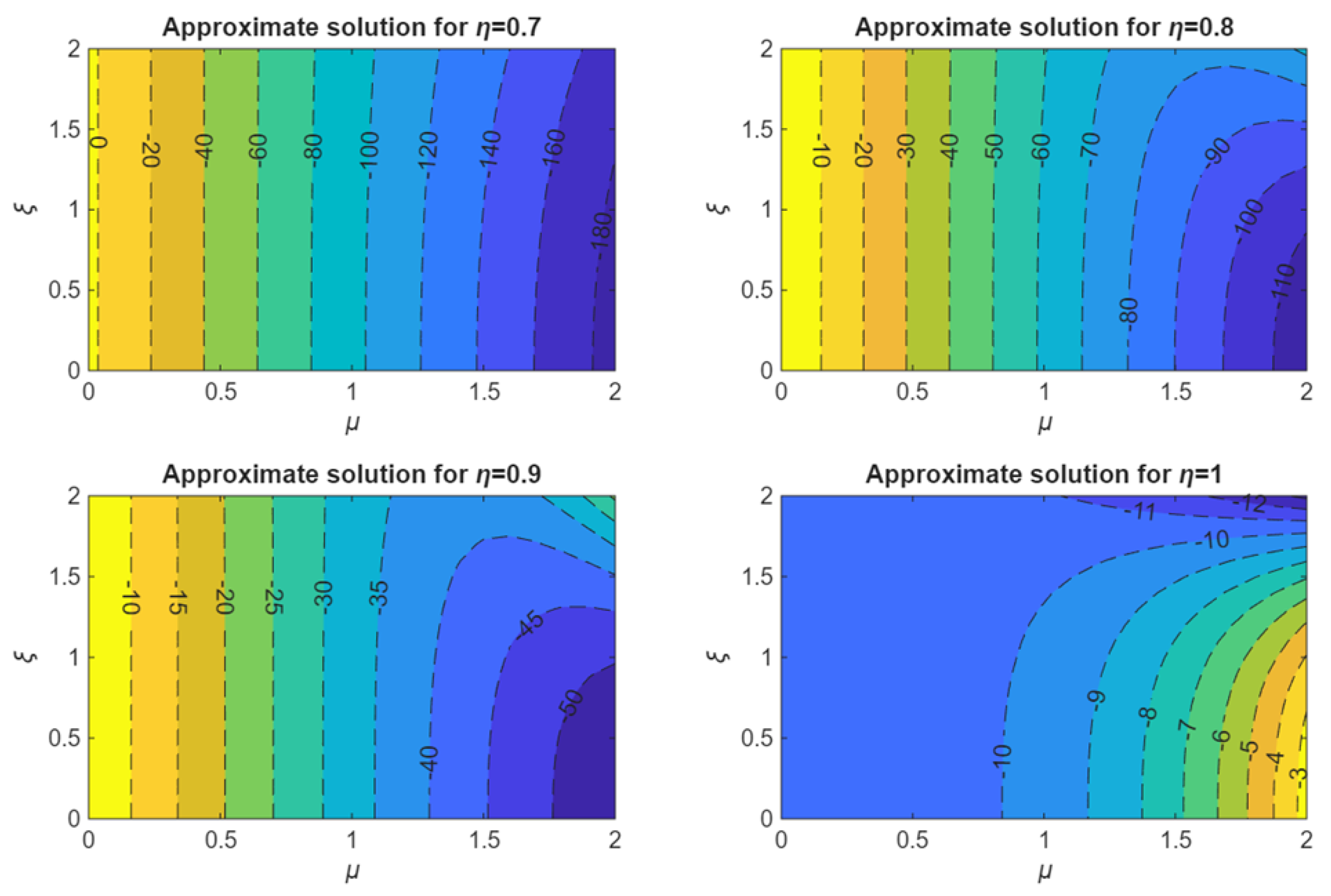
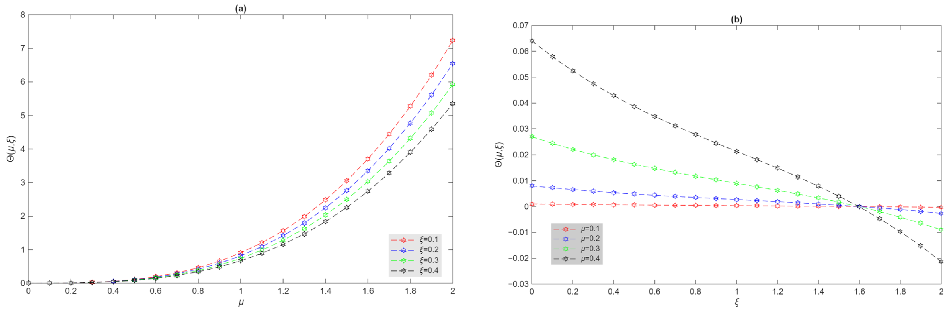
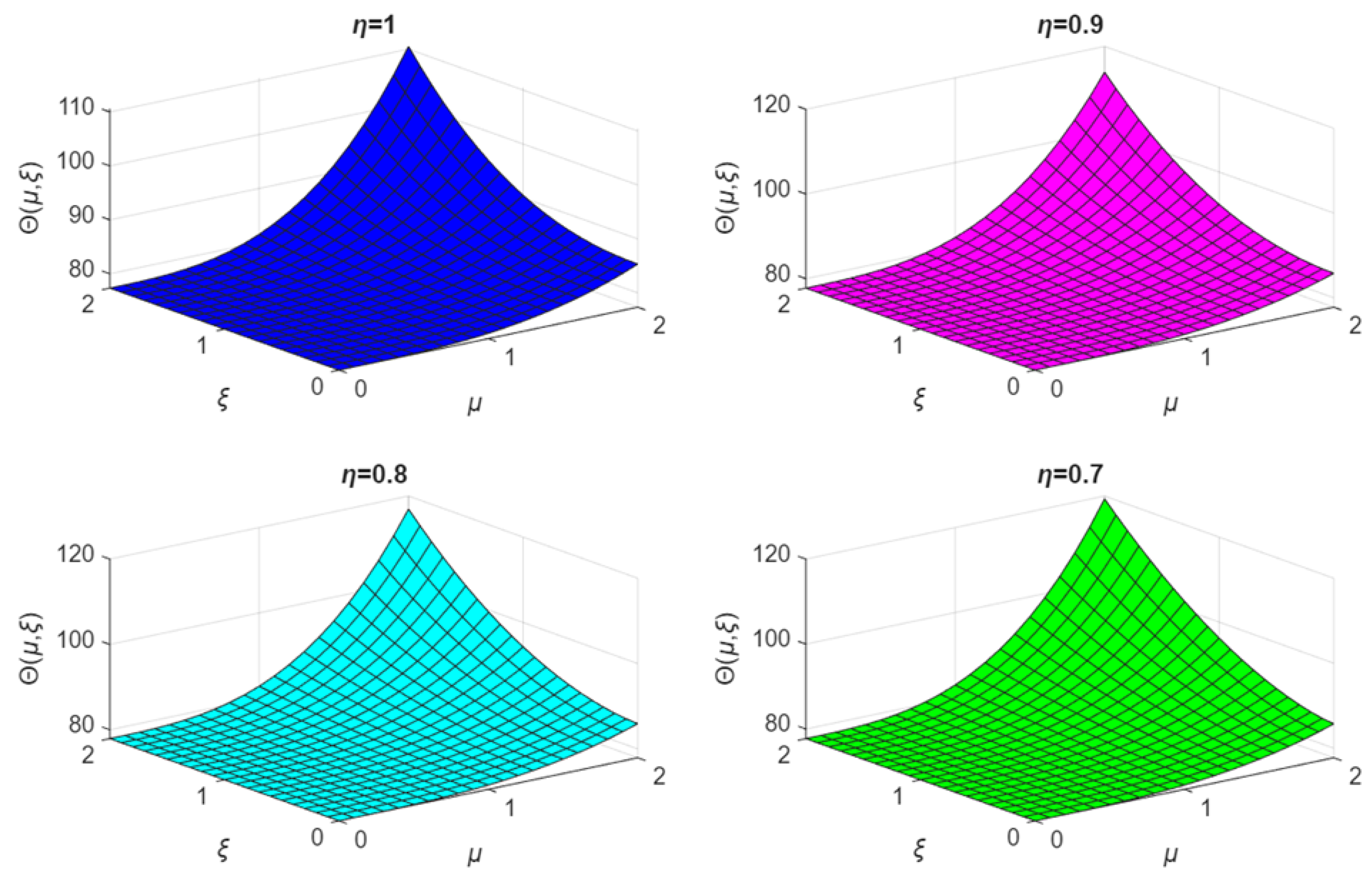
The graphical results for Example 4 are presented in Figure 8, Figure 9 and Figure 10. Figure 8 presents the three-dimensional surface plots of the YTADM solution for different fractional orders $\eta$, Figure 9 shows the corresponding contour plots, whereas Figure 10 illustrates the variation of the solution with respect to different values of $\xi$ and $\mu$.

Example 5.

Consider the nonlinear proportional DFPDE as follows:

$$\begin{array}{cc}\hfill {}^{C}D_{\xi }^{\eta }\Theta (\mu ,\xi )& ={\displaystyle \frac{{\partial }^2}{\partial {\mu }^2}}\Theta \left({\displaystyle \frac{\mu }{2}},{\displaystyle \frac{\xi }{2}}\right){\displaystyle \frac{\partial }{\partial \mu }}\Theta \left({\displaystyle \frac{\mu }{2}},{\displaystyle \frac{\xi }{2}}\right)+{\displaystyle \frac{23}{32}}\Theta (\mu ,\xi ),\hfill \end{array}$$

(75)

with the initial condition

$$\begin{array}{c}\hfill \Theta (\mu ,0)={\mu }^3,\end{array}$$

(76)

and the exact solution

$$\begin{array}{c}\hfill \Theta (\mu ,\xi )={\mu }^3{e}^{\xi }.\end{array}$$

(77)

Solution 5.

Applying the Yang transform to both sides of Equation (75) gives

$$\begin{array}{cc}\hfill \mathcal{R}(\mu ,\xi )& =\chi \Theta (\mu ,0)+{\chi }^{\eta }\mathsf{Y}\left[{\displaystyle \frac{{\partial }^2}{\partial {\mu }^2}}\Theta \left({\displaystyle \frac{\mu }{2}},{\displaystyle \frac{\xi }{2}}\right){\displaystyle \frac{\partial }{\partial \mu }}\Theta \left({\displaystyle \frac{\mu }{2}},{\displaystyle \frac{\xi }{2}}\right)+{\displaystyle \frac{23}{32}}\Theta (\mu ,\xi )\right].\hfill \end{array}$$

(78)

Applying the inverse Yang transform to Equation (78) gives

$$\begin{array}{cc}\hfill \Theta (\mu ,\xi )& =\Theta (\mu ,0)+{\mathsf{Y}}^{-1}\left[{\chi }^{\eta }\mathsf{Y}\left[{\displaystyle \frac{{\partial }^2}{\partial {\mu }^2}}\Theta \left({\displaystyle \frac{\mu }{2}},{\displaystyle \frac{\xi }{2}}\right){\displaystyle \frac{\partial }{\partial \mu }}\Theta \left({\displaystyle \frac{\mu }{2}},{\displaystyle \frac{\xi }{2}}\right)+{\displaystyle \frac{23}{32}}\Theta (\mu ,\xi )\right]\right].\hfill \end{array}$$

(79)

Assume that

$$\Theta (\mu ,\xi )={\displaystyle \sum _{n=0}^{\infty }}{\Theta }_n,{\displaystyle \frac{{\partial }^2}{\partial {\mu }^2}}\Theta \left({\displaystyle \frac{\mu }{2}},{\displaystyle \frac{\xi }{2}}\right){\displaystyle \frac{\partial }{\partial \mu }}\Theta \left({\displaystyle \frac{\mu }{2}},{\displaystyle \frac{\xi }{2}}\right)={\displaystyle \sum _{n=0}^{\infty }}{\mathcal{C}}_n,$$

(80)

where ${\mathcal{C}}_n$ is defined by

$$\begin{array}{cc}\hfill {\mathcal{C}}_0& ={\displaystyle \frac{{\partial }^2}{\partial {\mu }^2}}{\Theta }_0\left({\displaystyle \frac{\mu }{2}},{\displaystyle \frac{\xi }{2}}\right){\displaystyle \frac{\partial }{\partial \mu }}{\Theta }_0\left({\displaystyle \frac{\mu }{2}},{\displaystyle \frac{\xi }{2}}\right)\hfill \\ \hfill {\mathcal{C}}_1& ={\displaystyle \frac{{\partial }^2}{\partial {\mu }^2}}{\Theta }_0\left({\displaystyle \frac{\mu }{2}},{\displaystyle \frac{\xi }{2}}\right){\displaystyle \frac{\partial }{\partial \mu }}{\Theta }_1\left({\displaystyle \frac{\mu }{2}},{\displaystyle \frac{\xi }{2}}\right)+{\displaystyle \frac{{\partial }^2}{\partial {\mu }^2}}{\Theta }_1\left({\displaystyle \frac{\mu }{2}},{\displaystyle \frac{\xi }{2}}\right){\displaystyle \frac{\partial }{\partial \mu }}{\Theta }_0\left({\displaystyle \frac{\mu }{2}},{\displaystyle \frac{\xi }{2}}\right)\hfill \\ \hfill {\mathcal{C}}_2& ={\displaystyle \frac{{\partial }^2}{\partial {\mu }^2}}{\Theta }_0\left({\displaystyle \frac{\mu }{2}},{\displaystyle \frac{\xi }{2}}\right){\displaystyle \frac{\partial }{\partial \mu }}{\Theta }_2\left({\displaystyle \frac{\mu }{2}},{\displaystyle \frac{\xi }{2}}\right)+{\displaystyle \frac{{\partial }^2}{\partial {\mu }^2}}{\Theta }_1\left({\displaystyle \frac{\mu }{2}},{\displaystyle \frac{\xi }{2}}\right){\displaystyle \frac{\partial }{\partial \mu }}{\Theta }_1\left({\displaystyle \frac{\mu }{2}},{\displaystyle \frac{\xi }{2}}\right)+{\displaystyle \frac{{\partial }^2}{\partial {\mu }^2}}{\Theta }_2\left({\displaystyle \frac{\mu }{2}},{\displaystyle \frac{\xi }{2}}\right){\displaystyle \frac{\partial }{\partial \mu }}{\Theta }_0\left({\displaystyle \frac{\mu }{2}},{\displaystyle \frac{\xi }{2}}\right).\hfill \\ \hfill ⋮& \hfill \end{array}$$

Substituting Equation (80) into Equation (79), we obtain

$$\begin{array}{cc}\hfill {\displaystyle \sum _{n=0}^{\infty }}{\Theta }_n(\mu ,\xi )& =\Theta (\mu ,0)+{\mathsf{Y}}^{-1}\left[{\chi }^{\eta }\mathsf{Y}\left[{\displaystyle \sum _{n=0}^{\infty }}{\mathcal{C}}_n+{\displaystyle \frac{23}{32}}{\displaystyle \sum _{n=0}^{\infty }}{\Theta }_n\right]\right].\hfill \end{array}$$

(81)

Equating both sides of Equation (81), we have the following:

$$\left\{\begin{array}{c}{\Theta }_0(\mu ,\xi )={\mu }^3,\hfill \\ {\Theta }_1(\mu ,\xi )={\mathsf{Y}}^{-1}\left[{\chi }^{\eta }\mathsf{Y}\left[{\mathcal{C}}_0+{\displaystyle \frac{23}{32}}{\Theta }_0(\mu ,\xi )\right]\right],\hfill \\ ⋮\hfill \\ {\Theta }_{n+1}(\mu ,\xi )={\mathsf{Y}}^{-1}\left[{\chi }^{\eta }\mathsf{Y}\left[{\mathcal{C}}_n+{\displaystyle \frac{23}{32}}{\Theta }_n(\mu ,\xi )\right]\right],n\ge 1.\hfill \end{array}\right.$$

(82)

$$\begin{array}{cc}\hfill {\Theta }_1(\mu ,\xi )& ={\mathsf{Y}}^{-1}\left[{\chi }^{\eta }\mathsf{Y}\left[{\mathcal{C}}_0+{\displaystyle \frac{23}{32}}{\Theta }_0(\mu ,\xi )\right]\right]={\mathsf{Y}}^{-1}\left[{\chi }^{\eta }\mathsf{Y}\left[{\displaystyle \frac{9{\mu }^3}{32}}+{\displaystyle \frac{23{\mu }^3}{32}}\right]\right]\hfill \\ & ={\displaystyle \frac{{\mu }^3{\xi }^{\eta }}{\Gamma (\eta +1)}}.\hfill \end{array}$$

(83)

$$\begin{array}{cc}\hfill {\Theta }_2(\mu ,\xi )& ={\mathsf{Y}}^{-1}\left[{\chi }^{\eta }\mathsf{Y}\left[{\mathcal{C}}_1+{\displaystyle \frac{23}{32}}{\Theta }_1(\mu ,\xi )\right]\right]\hfill \\ & ={\mathsf{Y}}^{-1}\left[{\chi }^{\eta }\mathsf{Y}\left[{\displaystyle \frac{9{\mu }^3{\xi }^{\eta }}{2^{\eta +4}\Gamma (\eta +1)}}+{\displaystyle \frac{23{\mu }^3{\xi }^{\eta }}{32\Gamma (\eta +1)}}\right]\right]\hfill \\ & ={\displaystyle \frac{9{\mu }^3{\xi }^{2\eta }}{2^{\eta +4}\Gamma (2\eta +1)}}+{\displaystyle \frac{23{\mu }^3{\xi }^{2\eta }}{32\Gamma (2\eta +1)}}.\hfill \end{array}$$

(84)

$$\begin{array}{cc}\hfill {\Theta }_3(\mu ,\xi )& ={\mathsf{Y}}^{-1}\left[{\chi }^{\eta }\mathsf{Y}\left[{\mathcal{C}}_2+{\displaystyle \frac{23}{32}}{\Theta }_2(\mu ,\xi )\right]\right]\hfill \\ \hfill & ={\mathsf{Y}}^{-1}\left[{\chi }^{\eta }\mathsf{Y}\right[{\displaystyle \frac{81{\mu }^3{\xi }^{2\eta }}{2^{3\eta +8}\Gamma (2\eta +1)}}+{\displaystyle \frac{207{\mu }^3{\xi }^{2\eta }}{2^{2\eta +9}\Gamma (2\eta +1)}}+{\displaystyle \frac{9{\mu }^3{\xi }^{2\eta }}{2^{2\eta +5}\Gamma {(\eta +1)}^2}}\hfill \\ & +{\displaystyle \frac{207{\mu }^3{\xi }^{2\eta }}{2^{\eta +9}\Gamma (2\eta +1)}}+{\displaystyle \frac{529{\mu }^3{\xi }^{2\eta }}{1024\Gamma (2\eta +1)}}\left]\right]\hfill \\ \hfill & ={\displaystyle \frac{81{\mu }^3{\xi }^{3\eta }}{2^{3\eta +8}\Gamma (3\eta +1)}}+{\displaystyle \frac{207{\mu }^3{\xi }^{3\eta }}{2^{2\eta +9}\Gamma (3\eta +1)}}+{\displaystyle \frac{9{\mu }^3\Gamma (2\eta +1){\xi }^{3\eta }}{2^{2\eta +5}\Gamma {(\eta +1)}^2\Gamma (3\eta +1)}}\hfill \\ & +{\displaystyle \frac{207{\mu }^3{\xi }^{3\eta }}{2^{\eta +9}\Gamma (3\eta +1)}}+{\displaystyle \frac{529{\mu }^3{\xi }^{3\eta }}{1024\Gamma (3\eta +1)}}.\hfill \end{array}$$

(85)

Therefore, the YTADM solution is given by

$$\begin{array}{cc}\hfill \Theta (\mu ,\xi )& ={\mu }^3+{\displaystyle \frac{{\mu }^3{\xi }^{\eta }}{\Gamma (\eta +1)}}+{\displaystyle \frac{9{\mu }^3{\xi }^{2\eta }}{2^{\eta +4}\Gamma (2\eta +1)}}+{\displaystyle \frac{23{\mu }^3{\xi }^{2\eta }}{32\Gamma (2\eta +1)}}\hfill \\ \hfill & +{\displaystyle \frac{81{\mu }^3{\xi }^{3\eta }}{2^{3\eta +8}\Gamma (3\eta +1)}}+{\displaystyle \frac{207{\mu }^3{\xi }^{3\eta }}{2^{2\eta +9}\Gamma (3\eta +1)}}+{\displaystyle \frac{9{\mu }^3\Gamma (2\eta +1){\xi }^{3\eta }}{2^{2\eta +5}\Gamma {(\eta +1)}^2\Gamma (3\eta +1)}}\hfill \\ & +{\displaystyle \frac{207{\mu }^3{\xi }^{3\eta }}{2^{\eta +9}\Gamma (3\eta +1)}}+{\displaystyle \frac{529{\mu }^3{\xi }^{3\eta }}{1024\Gamma (3\eta +1)}}+\cdots \hfill \end{array}$$

(86)

and when $\eta =1$, the YTADM solution is reduced to

$$\begin{array}{c}\hfill \Theta (\mu ,\xi )={\mu }^3\left(1+\xi +{\displaystyle \frac{{\xi }^2}{2!}}+{\displaystyle \frac{{\xi }^3}{3!}}+\dots \right)={\mu }^3{e}^{\xi }.\end{array}$$

(87)

For the convergence analysis, we consider the case $\mu =0.3$, $\xi =0.3$ and $\eta =1$.

$$\begin{array}{cc}\hfill r_0& ={\displaystyle \frac{\parallel {\Theta }_1\parallel }{\parallel {\Theta }_0\parallel }}={\displaystyle \frac{\parallel 0.008100\parallel }{\parallel 0.027000\parallel }}=0.300000<1,\hfill \\ \hfill r_1& ={\displaystyle \frac{\parallel {\Theta }_2\parallel }{\parallel {\Theta }_1\parallel }}={\displaystyle \frac{\parallel 0.001215\parallel }{\parallel 0.008100\parallel }}=0.150000<1,\hfill \\ \hfill r_2& ={\displaystyle \frac{\parallel {\Theta }_3\parallel }{\parallel {\Theta }_2\parallel }}={\displaystyle \frac{\parallel 0.000121\parallel }{\parallel 0.001215\parallel }}=0.100000<1.\hfill \\ \hfill ⋮& \end{array}$$

Remark 5.

The above ratios are computed for the values $\mu =0.3$, $\xi =0.3$, and $\eta =1$. For $\eta =1$, the condition $r_n<1$ is satisfied for $0<\xi \le 0.8$.

For $\mu =0.2$, the YTADM solutions are computed for different values of the fractional order $\eta$. The corresponding numerical results are presented in

Table 7. YTADM solutions for various values $\eta =0.7, 0.8, 0.9, 1$ of Example 5.

$\mathit{\mu }$	$\mathit{\xi }$	$\mathit{\eta }=0.7$	$\mathit{\eta }=0.8$	$\mathit{\eta }=0.9$	$\mathit{\eta }=1$
	0.1	0.01006310	0.00951946	0.00912833	0.00884133
	0.2	0.01171730	0.01087587	0.01024875	0.00977067
	0.3	0.01339649	0.01229105	0.01144973	0.01079600
	0.4	0.01515036	0.01379838	0.01275084	0.01192533
0.2	0.5	0.01699771	0.01541319	0.01416386	0.01316667
	0.6	0.01894791	0.01714489	0.01569786	0.01452800
	0.7	0.02100633	0.01900026	0.01736062	0.01601733
	0.8	0.02317640	0.02098463	0.01915919	0.01764267
	0.9	0.02546041	0.02310249	0.02110013	0.01941200
	1.0	0.02786003	0.02535775	0.02318964	0.02133333

, while the comparison with the exact solutions and the corresponding absolute errors is given in

Table 8. Comparison between exact solutions and absolute errors of Example 5.

$\mathit{\mu }$	$\mathit{\xi }$	Exact Sol	Absolute Error	CPU Time
	0.1	0.00884137	$3.40113\times {10}^{-8}$	0.00035887
	0.2	0.00977122	$5.55399\times {10}^{-7}$	0.00012737
	0.3	0.01079887	$2.87046\times {10}^{-6}$	0.00011396
	0.4	0.01193460	$9.26425\times {10}^{-6}$	0.00011283
0.2	0.5	0.01318977	$2.31035\times {10}^{-5}$	0.00011246
	0.6	0.01457695	$4.89504\times {10}^{-5}$	0.00011450
	0.7	0.01611002	$9.26883\times {10}^{-5}$	0.00011213
	0.8	0.01780433	$1.61661\times {10}^{-4}$	0.00011237
	0.9	0.01967682	$2.64825\times {10}^{-4}$	0.00011196
	1.0	0.02174625	$4.12921\times {10}^{-4}$	0.00011171

.

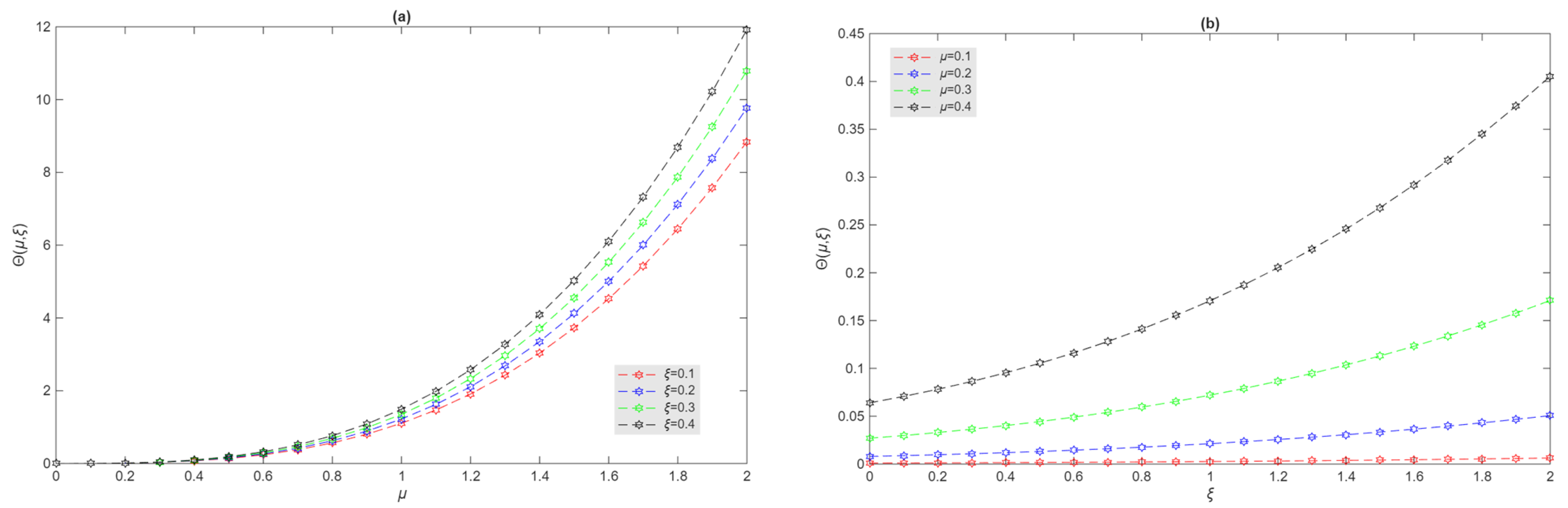
The graphical results for Example 4 are presented in Figure 11, Figure 12 and Figure 13. Figure 11 presents the three-dimensional surface plots of the YTADM solution for different fractional orders $\eta$, Figure 12 shows the corresponding contour plots, whereas Figure 13 illustrates the variation of the solution with respect to different values of $\xi$ and $\mu$.

6. Results and Discussion

The results indicate that the YTADM has been utilized with great success in various linear and nonlinear delay fractional partial differential equations (DFPDE) with the Caputo fractional derivative. In Examples 1 and 2, the iterative process gave the exact solution, whereas Table 1 and Table 2 demonstrate an absolute error of zero for all the selected values of $\mu$ and $\xi$. Correspondingly, two-dimensional and three dimensional plots illustrate the smoothness, stability and consistency of the solution obtained by the YTADM, indicating its ability to solve linear DFPDEs containing time delay terms as well as fractional power functions.

In Examples 3–5, nonlinear generalized Burgers-type DFPDEs were used, which contain time-proportional delay terms. The rapidly converging series solutions obtained by the YTADM closely represent the exact solutions. When $\eta =1$, the solution obtained from the YTADM represents the classical exact solutions to Equations (61), (74) and (87). The numerical solution produced using the YTADM remains very close to the exact solution for different fractional orders ($\eta =0.7, 0.8, 0.9, 1$), with very little absolute error throughout the entire computational range. While the approximation errors are generally small, Table 4 indicates that the error increases for larger parameter values, particularly near $\mu =0.2, \xi =1$ and $\eta =1$, owing to the truncation of the decomposition series to a finite number of terms.

Convergence analysis for Examples 3–5 illustrates that $r_n<1$, therefore establishing the convergence of the series provided by the YTADM. Three-dimensional graphics illustrate how the fractional-order parameter $\eta$ influences the behavior of the solution, demonstrating that there exist smooth surface solutions across the entire computational region. Contour plots provide additional evidence regarding the continuous nature and stability of the obtained solution for varying fractional-orders. Two-dimensional plots illustrate how the solution varies with respect to both $\mu$ and $\xi$, and overall, all the graphical results compare favorably with their respective exact solutions, thus providing strong evidence supporting the accuracy and dependability of the YTADM.

7. Conclusions

The obtained results demonstrate that the Yang Transform Adomian Decomposition Method (YTADM) provides a simple and computationally efficient framework for solving linear and nonlinear delay fractional partial differential equations. For the linear benchmark examples, the method reproduced the exact solutions within a few iterations, while for the nonlinear Burgers-type equations, it produced rapidly convergent and accurate approximate solutions. As expected for truncated decomposition methods, the approximation error may increase when only a finite number of series terms is retained. Moreover, the convergence analysis confirmed the convergence of the proposed method, and the graphical results illustrated the influence of the fractional-order parameter $\eta$ on the solution behavior.

In conclusion, the proposed YTADM is an effective semi-analytical tool for solving a broad class of one-dimensional linear and nonlinear delay fractional partial differential equations with constant-delay and proportional-delay terms. The proposed framework may also be extended to multidimensional and coupled delay fractional partial differential equations, which will be considered in future work.

References

1. Kumar, D.; Seadawy, A.R.; Joardar, A.K. Modified Kudryashov method via new exact solutions for some conformable fractional differential equations arising in mathematical biology. Chin. J. Phys. 2018, 56, 75–85. [Google Scholar] [CrossRef]
2. Bonfanti, A.; Kaplan, J.L.; Charras, G.; Kabla, A. Fractional viscoelastic models for power-law materials. Soft Matter 2020, 16, 6002–6020. [Google Scholar] [CrossRef] [PubMed]
3. Prakasha, D.G.; Veeresha, P.; Baskonus, H.M. Residual power series method for fractional Swift–Hohenberg equation. Fractal Fract. 2019, 3, 9. [Google Scholar] [CrossRef]
4. Wang, X.; Wang, H. Contemporary delay differential equation models and analysis in mathematical biology. In Contemporary Research in Mathematical Biology–Modeling, Computation and Analysis; World Scientific: Singapore, 2022. [Google Scholar]
5. Zhmud, V.; Dimitrov, L. Using the fractional differential equation for the control of objects with delay. Symmetry 2022, 14, 635. [Google Scholar] [CrossRef]
6. Chai, L.; Fei, S. Memory state-feedback stabilization for a class of time-delay systems with a type of adaptive strategy. J. Appl. Math. 2013, 2013, 319415. [Google Scholar] [CrossRef]
7. Xie, X.; Zhang, H.; Liu, T. On designing memory state feedback controller for linear systems with interval time-varying delay. J. Control Theory Appl. 2010, 8, 479–484. [Google Scholar] [CrossRef]
8. Ouyang, Z. Existence and uniqueness of the solutions for a class of nonlinear fractional-order partial differential equations with delay. Comput. Math. Appl. 2011, 61, 860–870. [Google Scholar] [CrossRef]
9. Rihan, F.A. Computational methods for delay parabolic and time-fractional partial differential equations. Numer. Methods Partial Differ. Equ. 2010, 26, 1556–1571. [Google Scholar] [CrossRef]
10. Prakash, P.; Choudhary, S.; Daftardar-Gejji, V. Exact solutions of generalized nonlinear time-fractional reaction–diffusion equations with time delay. Eur. Phys. J. Plus 2020, 135, 490. [Google Scholar] [CrossRef]
11. Ghanbari, B. A fractional system of delay differential equations with nonsingular kernels in modeling hand-foot-mouth disease. Adv. Differ. Equ. 2020, 2020, 536. [Google Scholar] [CrossRef] [PubMed]
12. Ahmed, S.S.; Amin, M.B.M.; Hamasalih, S.A. Laplace Adomian decomposition and modified Laplace Adomian decomposition methods for solving linear Volterra integro-fractional differential equations with constant multi-time retarded delay. J. Univ. Babylon Pure Appl. Sci. 2019, 27, 35–53. [Google Scholar]
13. Sherman, M.; Kerr, G.; González-Parra, G. Comparison of symbolic computations for solving linear delay differential equations using the Laplace transform method. Math. Comput. Appl. 2022, 27, 81. [Google Scholar] [CrossRef]
14. Kaplan, A.G.; Ablay, M.V. Exact solution of the Bagley–Torvik equation using Laplace transform method. Southeast Asian Bull. Math. 2022, 46, 729–736. [Google Scholar]
15. Morales-Delgado, V.F.; Gómez-Aguilar, J.F.; Yépez-Martínez, H.; Baleanu, D.; Escobar-Jimenez, R.F.; Olivares-Peregrino, V.H. Laplace homotopy analysis method for solving linear partial differential equations using a fractional derivative with and without kernel singular. Adv. Differ. Equ. 2016, 2016, 164. [Google Scholar] [CrossRef]
16. Nuruddeen, R.I. Analytical solution for time-fractional diffusion equation by Aboodh decomposition method. J. King Saud Univ. Sci. 2017, 29, 52–57. [Google Scholar]
17. Merdan, M.; Şahin, Y.; Açıkgöz, P. The novel numerical solutions for the Caputo–Fabrizio fractional Newell–Whitehead–Segel equation by using Aboodh–ADM. Preprint 2024. [Google Scholar] [CrossRef] [PubMed]
18. Al-Aati, A.; Al-Sharai, W.M. Exact solution of linear and nonlinear system of partial differential equations by double Aboodh–Shehu and Adomian decomposition method. Albaydha Univ. J. 2023, 5, 332–346. [Google Scholar] [CrossRef]
19. Noor, S.; Albalawi, W.; Shah, R.; Shafee, A.; Ismaeel, S.M.E.; El-Tantawy, S.A. A comparative analytical investigation for some linear and nonlinear time-fractional partial differential equations in the framework of the Aboodh transformation. Front. Phys. 2024, 12, 1374049. [Google Scholar] [CrossRef]
20. Ali, M.A.; Merdan, M. Solution of time-fractional coupled Burgers equations by the Yang transform Adomian decomposition method. J. Appl. Math. 2026, 2026 1, 1388808. [Google Scholar] [CrossRef]
21. Ali, M.A.; Merdan, M. Approximate analytical solutions of the time-fractional Swift–Hohenberg equation via Yang transform Adomian decomposition method. J. Appl. Math. 2026, 2026 1, 5815304. [Google Scholar] [CrossRef]
22. Shah, R.; Khan, H.; Kumam, P.; Arif, M.; Baleanu, D. Natural transform decomposition method for solving fractional-order partial differential equations with proportional delay. Mathematics 2019, 7, 532. [Google Scholar] [CrossRef]
23. Bekela, A.S.; Belachew, M.T.; Wole, G.A. A numerical method using Laplace-like transform and variational theory for solving time-fractional nonlinear partial differential equations with proportional delay. Adv. Differ. Equ. 2020, 2020, 586. [Google Scholar] [CrossRef]
24. Bekela, A.S.; Woldaregay, M.M. Natural transform method with modified ADM for nonlinear time-fractional PDEs with proportional delay. Preprint 2025. [Google Scholar] [CrossRef] [PubMed]
25. Alsulami, M.; Al-Mazmumy, M.; Al-Yazidi, N.S. Effective iterative procedure for delay fractional partial differential equations using Sumudu decomposition method. Symmetry 2026, 18, 407. [Google Scholar] [CrossRef]
26. Hosseinpour, S.; Nazemi, A.; Tohidi, E. A new approach for solving a class of delay fractional partial differential equations. Mediterr. J. Math. 2018, 15, 218. [Google Scholar] [CrossRef]
27. Nouri, K.; Nazari, M.; Torkzadeh, L. Numerical approximation of the system of fractional differential equations with delay and its applications. Eur. Phys. J. Plus 2020, 135, 341. [Google Scholar] [CrossRef]
28. Choudhary, R.; Singh, S.; Kumar, D. A second-order numerical scheme for the time-fractional partial differential equations with a time delay. Comput. Appl. Math. 2022, 41, 114. [Google Scholar] [CrossRef]
29. Alsuyuti, M.M.; Doha, E.H.; Bayoumi, B.I.; Ezz-Eldien, S.S. Robust spectral treatment for time-fractional delay partial differential equations. Comput. Appl. Math. 2023, 42, 159. [Google Scholar] [CrossRef]
30. Kamran; Athar, K.; Khan, Z.A.; Haque, S.; Mlaiki, N. Analysis of time-fractional delay partial differential equations using a local radial basis function method. Fractal Fract. 2024, 8, 683. [Google Scholar] [CrossRef]
31. Ala’yed, O. Modified two-dimensional differential transform method for solving proportional delay partial differential equations. Results Control Optim. 2024, 17, 100499. [Google Scholar] [CrossRef]
32. Liaqat, M.I.; Khan, A.; Akgül, A.; Ali, M.S. A novel numerical technique for fractional ordinary differential equations with proportional delay. J. Funct. Spaces 2022, 2022, 6333084. [Google Scholar] [CrossRef]
33. Sabermahani, S.; Ordokhani, Y.; Yousefi, S.-A. Fractional-order Fibonacci-hybrid functions approach for solving fractional delay differential equations. Eng. Comput. 2020, 36, 795–806. [Google Scholar] [CrossRef]
34. Ganie, A.H.; AlBaidani, M.M.; Khan, A. A comparative study of the fractional partial differential equations via novel transform. Symmetry 2023, 15, 1101. [Google Scholar] [CrossRef]
35. Ganie, A.H.; Mofarreh, F.; Khan, A. A novel analysis of the time-fractional nonlinear dispersive K(m, n, 1) equations using the homotopy perturbation transform method and Yang transform decomposition method. AIMS Math. 2024, 9, 1877–1898. [Google Scholar]
36. Abdali, M.H. An iterative approach for solving fractional differential equations using YJ Adomian decomposition method. Int. J. Appl. Math. 2025, 38, 1244–1256. [Google Scholar] [CrossRef]
37. Ramadan, M.A.; Abd El-Latif, M.A.A.; Alqarni, M.Z. An integrated Laplace transform and accelerated Adomian decomposition approach for solving time-fractional nonlinear partial differential equations. Electron. Res. Arch. 2025, 33, 4398–4434. [Google Scholar] [CrossRef]
38. Şahin, Y.; Merdan, M.; Açıkgöz, P. Development of a hybrid technique for solving the Newell–Whitehead–Segel equation using the Caputo–Fabrizio derivative. Eng. Comput. 2025, 43, 1470–1495. [Google Scholar] [CrossRef]
39. Al-Griffi, T.A.J.; Al-Saif, A.-S.J. Yang transform–homotopy perturbation method for solving a non-Newtonian viscoelastic fluid flow on the turbine disk. Z. Angew. Math. Mech. 2022, 102, e202100116. [Google Scholar] [CrossRef]
40. Merdan, M.; Oral, P. On the solutions of nonlinear fractional Klein–Gordon equation by means of local fractional derivative operators. Turk. J. Math. Comput. Sci. 2016, 5, 19–31. [Google Scholar]
41. Singh, B.K.; Kumar, P. Homotopy perturbation transform method for solving fractional partial differential equations with proportional delay. SeMA J. 2018, 75, 111–125. [Google Scholar] [CrossRef]
42. Dogan, D.D.; Konuralp, A. Fractional variational iteration method for time-fractional nonlinear functional partial differential equation having proportional delays. Therm. Sci. 2018, 22, S33–S46. [Google Scholar] [CrossRef]
43. Farhood, A.K.; Mohammed, O.H. Homotopy perturbation method for solving time-fractional nonlinear variable-order delay partial differential equations. Partial Differ. Equ. Appl. Math. 2023, 7, 100513. [Google Scholar] [CrossRef]
44. Naeem, M.; Yasmin, H.; Shah, R.; Shah, N.A.; Chung, J.D. A comparative study of fractional partial differential equations with the help of Yang transform. Symmetry 2023, 15, 146. [Google Scholar] [CrossRef]
45. Ganie, A.H.; Khan, A.; Alharthi, N.S.; Tolasa, F.T.; Jeelani, M.B. Comparative analysis of time-fractional coupled system of shallow-water equations including Caputo’s fractional derivative. J. Math. 2024, 2024, 2440359. [Google Scholar] [CrossRef]
46. Sedeeg, A.K.; Mahamoud, Z.I.; Saadeh, R. Using double integral transform (Laplace-ARA transform) in solving partial differential equations. Symmetry 2022, 14, 2418. [Google Scholar] [CrossRef]
47. Veeresha, P.; Prakasha, D.G.; Baskonus, H.M. Solving smoking epidemic model of fractional order using a modified homotopy analysis transform method. Math. Sci. 2019, 13, 115–128. [Google Scholar] [CrossRef]
48. Kumar, D.; Singh, J.; Baleanu, D. A new analysis for fractional model of regularized long-wave equation arising in ion acoustic plasma waves. Math. Methods Appl. Sci. 2017, 40 15, 5642–5653. [Google Scholar] [CrossRef]
49. Magreñán, A.A. A new tool to study real dynamics: The convergence plane. Appl. Math. Comput. 2014, 248, 215–224. [Google Scholar] [CrossRef]
Figure 1. 3-D surface plots of the YTADM solution Θ ( μ , ξ ) of Example 1 for η = 1 .
Symmetry 18 01242 g001
Figure 2. (a) Variation of Θ ( μ , ξ ) at ξ = 0.1 ,   0.2 ,   0.3 ,   0.4 of Example 1. (b) Variation of Θ ( μ , ξ ) at μ = 0.1 ,   0.2 ,   0.3 ,   0.4 of Example 1.
Symmetry 18 01242 g002
Figure 3. 3-D surface plots of the YTADM solution Θ ( μ , ξ ) of Example 2 for η = 1 .
Symmetry 18 01242 g003
Figure 4. (a) Variation of Θ ( μ , ξ ) at ξ = 0.1 ,   0.2 ,   0.3 ,   0.4 of Example 2. (b) Variation of Θ ( μ , ξ ) at μ = 0.1 ,   0.2 ,   0.3 ,   0.4 of Example 2.
Symmetry 18 01242 g004
Figure 5. 3-D surface plots of the approximate YTADM solutions of Example 3 for various fractional orders η = 0.7 ,   0.8 ,   0.9 ,   1 , illustrating the influence of the fractional-order parameter on the solution behavior.
Symmetry 18 01242 g005
Figure 6. Contour plots of the solutions Θ ( μ , ξ ) for fractional orders η = 0.7 ,   0.8 ,   0.9 ,   1 of Example 3.
Symmetry 18 01242 g006
Figure 7. (a) Variation of Θ ( μ , ξ ) at ξ = 0.1 ,   0.2 ,   0.3 ,   0.4 of Example 3. (b) Variation of Θ ( μ , ξ ) at μ = 0.1 ,   0.2 ,   0.3 ,   0.4 of Example 3.
Symmetry 18 01242 g007
Figure 8. 3-D surface plots of the approximate YTADM solutions of Example 4 for various fractional orders η = 0.7 ,   0.8 ,   0.9 ,   1 , illustrating the influence of the fractional-order parameter on the solution behavior.
Symmetry 18 01242 g008
Figure 9. Contour plots of the solutions Θ ( μ , ξ ) for fractional orders η = 0.7 ,   0.8 ,   0.9 ,   1 of Example 4.
Symmetry 18 01242 g009
Figure 10. (a) Variation of Θ ( μ , ξ ) at ξ = 0.1 ,   0.2 ,   0.3 and 0.4 of Example 4. (b) Variation of Θ ( μ , ξ ) at μ = 0.1 ,   0.2 ,   0.3 and 0.4 of Example 4.
Symmetry 18 01242 g010
Figure 11. 3-D surface plots of the approximate YTADM solutions of Example 5 for various fractional orders η = 0.7 ,   0.8 ,   0.9 ,   1 , illustrating the influence of the fractional-order parameter on the solution behavior.
Symmetry 18 01242 g011
Figure 12. Contour plots of the solutions Θ ( μ , ξ ) for fractional orders η = 0.7 ,   0.8 ,   0.9 ,   1 of Example 5.
Symmetry 18 01242 g012
Figure 13. (a) Variation of Θ ( μ , ξ ) at ξ = 0.1 ,   0.2 ,   0.3 and 0.4 of Example 5. (b) Variation of Θ ( μ , ξ ) at μ = 0.1 ,   0.2 ,   0.3 and 0.4 of Example 5.
Symmetry 18 01242 g013