Symmetry-Driven Enhanced Auxiliary Classifier GAN for Data-Efficient Breast Tumor Classification

Abstract

The intricate nature of multi-class histopathological images, combined with pronounced class imbalances, complicates automated breast cancer diagnosis and demands AI models capable of generalizing well beyond often limited training data. To address these challenges, this paper explores the generative modeling capability of a symmetry-driven enhanced auxiliary classifier GAN (LSWACGAN) as an all-in-one, data-efficient framework for breast cancer histopathological image classification. LSWACGAN incorporates the Wasserstein loss with gradient penalty to promote greater training stability by mitigating overfitting and preventing vanishing gradients. Assigning smooth category labels to generated samples further helps alleviate the mode collapse problem. The proposed framework brings together three types of symmetry to improve its reliability: the inherent metric symmetry of the Wasserstein distance, the structural symmetry within the auxiliary classifier GAN, and the architectural symmetry between the generator and discriminator networks. Extensive experiments conducted on the well-known BreakHis dataset, supplemented by a thorough ablation study, demonstrate the framework’s competitive edge in a lower-data regime. For binary classification, LSWACGAN closely matches or slightly outperforms leading benchmarks on most selected evaluation metrics. Conversely, in the multi-class scenario, it emerges as a clear forerunner, consistently producing superior results and maintaining robust performance across varying magnification levels.

1. Introduction

Breast cancer remains a major global health concern, ranking as the second leading malignancy worldwide. It accounts for approximately 11.5% of all new cancer cases reported annually [1]. In Europe alone, the year 2030 is projected to see around 406,825 new instances of breast cancer among women, alongside an estimated 4942 new breast cancer diagnoses in men [2]. Notably, breast cancer constitutes nearly a quarter (23.8%) of all new cancer in women, making it the most ubiquitous cancer type amongst this population globally. With its incidence continuously rising, the importance of timely detection cannot be overstated, as it has an essential role in enhancing survival rates and mitigating the morbidity linked to breast cancer. This is particularly significant given the heterogeneous nature of the disease—which comprises various subtypes, each characterized by unique biochemical, histological, and clinical features—presenting many challenges in its diagnosis, treatment and prognosis.

Screening programs are indispensable for breast cancer detection in its preclinical stages, enabling less invasive yet effective treatment options that significantly enhance patients’ outcomes in terms of both survival and quality of life. These programs primarily rely on various radiological methods—from X-rays to modern modalities like mammography, ultrasound, positron emission tomography (PET), computed tomography (CT) and magnetic resonance imaging (MRI)—to uncover early indicators of neoplasms, including microcalcifications, architectural distortions, and solid masses [3,4,5]. However, these non-invasive techniques have limitations, which may lead to unnecessary or inappropriate handling and potentially serious ramifications. In cases of uncertainty, a definitive diagnosis is obtained through biopsy. This procedure entails collecting tissue samples, preparing them on glass slides, staining them, and subsequently examining the samples under a microscope by pathologists to identify cancerous cells. Though this method offers a high level of confidence, it is time-consuming and strongly dependent on pathologists’ expertise. Medical specialists are required to have exceptional focus and consistent performance, but being human, they are susceptible to factors such as fatigue, bias and potential distractions. In this context, well-trained AI algorithms can serve either as fail-check mechanisms or as real-time assistants to enhance the sensitivity and specificity of human operators’ interpretations.

Recent advances in machine learning, especially deep learning, have sparked groundbreaking progress across a range of complex tasks, particularly in the realm of speech and image processing. These advances stem from a data-centric approach that focuses on hierarchical feature learning, in contrast to traditional methods that rely on fixed, hardwired feature representations.

Table A1. Summary of recent studies on breast cancer histopathological image classification using deep learning techniques (2025–2026).

Study	Dataset	Methodology	Training Details	Data Regime	Acuracy	Limitation
Alzoubi et al. (2026) [62]	BreakHis	The combination of pretrained ResNet-50 for deep feature extraction and Salp Swarm Algorithm (SSA) for dimensionality reduction	Image preprocessing to normalize the dataset due to the imbalance; a smaller number of poor-quality images compared to high-quality ones was introduced to guarantee that the model evaluates both categories equally	Not enough information	$96.45\%$	Limited to binary classification
Aneesha and Zoheir (2026) [63]	IDC	An optimized lightweight CNN derived from the reference BCDNet architecture, with progressive regularization and Global Average Pooling (GAP)	IDC(+)/No Cancer patch-based classification; data augmentation; L2 regularization and class weighting to handle class imbalance	High	$91.38\%$	Domain-specific; not built for whole-slide image analysis
Zeng et al. (2026) [64]	BreakHis BACH BCI UCSB	A novel framework that combines a pathology-informed augmentation pipeline (HistoAugment) to counter class imbalance, a Center-Border Partition Module (CBPM) for spatially differentiated feature extraction, and a dynamically fused dual-branch network (DFD-Net)	No specific details provided	BreakHis: Low BACH: Low BCI: Low UCSB: Low	BreakHis: $92.10\%$ BACH: $82.50\%$ BCI: $93.76\%$ UCSB: −	Limited to binary classification; lacks interpretability
Bohra et al. (2026) [65]	BreakHis	A multi-scale framework combining the Lifting Wavelet Transform (LWT) and multi-path CNN	Data augmentation; various magnification levels combined using Haar wavelet filter	Moderate	$99.34\%$	Limited to binary classification; computationally heavy
Desai and Mahto (2025) [66]	BreakHis	An automated deep learning-based framework for multi-class classification of breast cancer subtypes, leveraging various ResNet architectures (ResNet-18, ResNet-34, and ResNet-50)	Data augmentation; random shuffling to handle class imbalance	Not enough information	$92.42\%$	Limited interpretability
Wakili et al. (2025) [67]	BreakHis BACH	DenseNet-FPA: A hybrid framework that integrates pretrained DenseNet-201 for hierarchical feature extraction with Flower Poliniation Algorithm (FPA) for optimized feature selection	Data augmentation; images from various magnification levels mixed together	BreakHis: Moderate BACH: Low	BreakHis: $99.32\%$ BACH: $96.00\%$	Limited to binary classification
Alshehri (2025) [68]	BreakHis IDC	BreNet: An ensemble combining three pretrained CNN bakbones (DenseNet-201, ResNet-50, and EfficientNet-B0) with channel and spatial attention mechanisms	Adaptive Synthetic (ADASYN) oversampling to counter class imbalance; five-fold patient-wise cross-validation	BreakHis: Moderate IDC: High	BreakHis: $99.96\%$ IDC: $88.26\%$	Limited to binary classification
Arshad et al. (2025) [69]	IDC	HistoDX: A customized CNN based on EfficientV2-B3 architecture	IDC(+)/No Cancer patch-based classification; oversampling and weighted loss used to balance training set; minimal augmentation	High	$97.00\%$	Limited to $40\times$ magnification; not built for whole-slide image analysis
Zhao et al. (2025) [70]	BreakHis BACH	HoRFNet: An innovative receptive field network integrating multi-branch convolutions and dilated convolutional layers with high-order statistical modeling streams	Data augmentation	BreakHis: Not enough information BACH: Low	BreakHis: $99.50\%$ BACH: $88.75\%$	Limited to binary classification
Jia et al. (2025) [71]	BreakHis BACH	DenLSNet-C: A novel hybrid deep learning model that integrates an improved DenseNet-201—featuring Squeeze-and-Excitation (SE) and iterative Convolutional Feature Fusion (iCFF) blocks—for spatial feature extraction, with a Long Short-Term Memory (LSTM) network for sequence-based context	Data augmentation	BreakHis: Not enough information BACH: Low	BreakHis: $96.28\%$ BACH: $96.88\%$	Limited interpretability
Chikkala et al. (2025) [72]	BreakHis	An innovative method utilizing Bidirectional Recurrent Neural Networks (BRNN), made up of four unique elements: pretrained ResNet-50 for transfer learning, the Gated Recurrent Unit (GRU), the residual collaborative branch, and the feature fusion module based on Adagard optimization algorithm	Data augmentation	Not enough information	$97.25\%$	Limited interpretability, computationally heavy due to multiple branches and feature fusion strategy

in Appendix A showcases a curated selection of the most prominent achievements, attained using state-of-the-art deep learning models (e.g., ResNet, DenseNet, EfficientNet). The table synthesizes key insights from relevant open-access studies, published within the last 18 months, outlining their methodologies, training protocols, data regimes, results, and potential limitations.

As highlighted in Table A1, the triumphs of supervised deep learning algorithms come with a price of high computational demands, prolonged training times, and a hunger for vast amounts of annotated data to train large networks with billions of parameters. A notable impediment to the use of supervised deep learning in medical imaging analysis [6] is the scarcity of extensive, well-annotated datasets, exacerbated by the unstructured nature of healthcare data, which requires meticulous acquisition and curation supervised by highly trained medical specialists, who are often stretched thin due to patient care responsibilities. Additionally, privacy and ethical concerns hinder the sharing of medical images within the open-source domain. On top of this, supervised deep neural networks are notoriously sensitive to any dataset imbalances, leading to issues like overfitting when trained on limited data. Different strategies—including data augmentation, multi-task learning, transfer learning, and few-shot learning—have been adopted to mitigate these challenges to a certain degree.

Despite deep neural networks having achieved remarkable feats, often surpassing human performance on numerous tasks, human ability to learn concepts, entities, or phenomena from only one or a few instances, even when the context gets significantly altered, remains largely unattainable. This uncanny skill—typically linked to the unique capacity of the human brain, which is able to not only memorize but also reconstruct new scenarios from partial, noisy, and uncertain information—can be effectively imparted into neural networks through the use of unsupervised generative modeling approaches that have shown great promise in a variety of applications.

Unlike traditional models that attempt to predict class labels, generative models aim to represent the underlying data distribution and, by doing so, they can capture the causal factors behind the data-generation process. Generative models can synthesize new information based on the learned causal attributes, allowing them to identify novel instances of known occurrences. Consequently, knowledge gleaned from a limited set of training examples can be repurposed to regenerate subtle anatomical and pathological structures that may have been missed in lower-quality medical images, while simultaneously filtering out extraneous noise that lacks relevance to the original image signature. This not only enhances data efficiency but also bolsters the generalization capabilities of the network.

Diffusion models [7], variational autoencoders (VAEs) [8], and generative adversarial networks (GANs) [9] are the three most prominent generative frameworks, applied in diverse domains ranging from image, audio and video synthesis to natural language processing. Diffusion models are characterized by a fixed forward diffusion process paired with a learnable reverse diffusion process. Unlike VAEs and GANs, which generate samples at once, diffusion models create samples through a step-by-step approach. The model first creates a rough image structure, subsequently refining it by adding detailed features on top. This layered method allows diffusion models to produce high-fidelity outputs, but the process is computationally heavy, requiring multiple iterations to gradually generate samples, which makes them much slower compared to GANs and VAEs. Alternatively, VAEs are relatively straightforward to implement and train. However, they rely on an assumption regarding the posterior distribution to adeptly approximate the true data distribution, resulting in inferior-quality reconstructions. GANs operate on a contrasting principle to diffusion models and VAEs as they do not utilize an inference network. Instead, they rely on a unique adversarial training process akin to a two-player game involving a generator and a discriminator, which not only enhances the discriminator’s proficiency in differentiating between genuine samples and their synthetic counterparts but also empowers the generator to produce high-quality outputs that closely mimic the true data distribution. Although GANs are tricky to train, by carefully selecting network parameters, loss functions, and optimization algorithms, their training stability and modeling ability can be significantly improved, all the while alleviating the risks associated with mode collapse.

While standard GANs and their variants are nowadays extensively employed for data augmentation, conditional synthesis, super-resolution, and style transfer, to the best of our knowledge, there is little reported research exploring end-to-end GAN-based supervised classification specifically in terms of breast cancer histopathological subtype recognition. The auxiliary classifier GAN stands out due to its inherent classification capacity, thanks to its architecture that includes an auxiliary classifier branch. By providing disentangled latent codes in the form of one-hot-encoded class labels alongside a noise vector, the auxiliary classifier GAN effectively models the data distribution. This approach facilitates the learning of representations that are distinct across various target classes, positioning the network as particularly suited for classification tasks.

In this paper, we utilize the auxiliary classifier branch of a symmetry-driven enhanced auxiliary classifier GAN—termed LSWACGAN—to perform both binary and eight-class breast tumor subtype classification based on histopathological images. The generator and discriminator within LSWACGAN are trained in an adversarial manner, by taking advantage of unsupervised representation learning. To prevent the model from becoming overly confident, generated samples are assigned smooth rather than hard labels during training, which not only improves the stability of the learning process but also allows these samples to serve as a form of regularization. Furthermore, the cross-entropy (CE) loss is amplified by integrating it with the Wasserstein loss, which includes a gradient penalty term, to enhance the classification of generated images. Contrary to conventional CE loss, the Wasserstein loss encourages the generator to produce samples that are “close” to the real data by increasing the gap between scores for real and generated data, leading to a smoother training process and preventing the generator from getting stuck producing repetitive samples. Once training is complete, the discriminator component is decoupled from LSWACGAN and configured to function as a standalone classifier.

The systematic symmetry concepts in the LSWACGAN are mainly reflected in threefold: the metric symmetry of the Wasserstein distance, the equal treatment in the auxiliary classifier GAN, and the mirrored designs of the generator and discriminator networks. At the core of the framework lies the Kantorovich–Rubinstein duality [10], which formulates distance calculation as a symmetric metric space over 1-Lipschitz continuous functions. This symmetric metric space enables continuous, non-saturating gradients even when the real and fake data manifolds are disjoint, thereby greatly reducing pitfalls like mode collapse. The Wasserstein distance adheres to the symmetry axiom, ensuring that the discriminator evaluates the discrepancy between the two distributions identically, regardless of which is designated as real or generated. The auxiliary classification branch introduces another distinct form of symmetry by treating real and fake data with equal scrutiny. The discriminator acts simultaneously as both a critic and a classifier, compelling the generator to not only mimic the underlying data manifold but also align with categorical boundaries. Symmetrical gradient updates reinforce class-conditional fidelity. This dual-objective setup maintains class symmetry, which is crucial for balanced generation across categories and prevents the model from disproportionately favoring any particular class. Furthermore, the LSWACGAN employs twin-like network structures, which promote spatial and feature symmetry by coordinating down-sampling and up-sampling processes between the generator and discriminator.

To summarize, the key contributions of this paper are laid out as follows:

(a)

Designing and implementing an auxiliary classifier GAN-based model for breast cancer diagnosis, focusing on classifying benign and malignant cases with high accuracy using histopathological images.

(b)

Integrating a Wasserstein loss into the auxiliary classifier GAN to provide more informative gradients to the generator network, thus enabling it to learn complex distributions in high-dimensional spaces.

(c)

Conducting a thorough evaluation of the model’s performance, benchmarking it against two cutting-edge pretrained, fine-tuned, deep neural network architectures—namely, DenseNet-121 and EfficientNet-B0—to showcase its efficacy on a small-scale dataset across multiple scenarios, ranging from binary to multi-class.

The remainder of this paper is organized as follows. Section 2 provides a succinct overview of the relevant literature, while Section 3 describes the proposed models and delineates the methodology employed. The experimental setup, along with the dataset utilized for this research, is thoroughly elaborated in Section 4. The results are presented and discussed in Section 5. Finally, Section 6 provides a paper summary and highlights potential avenues for future research.

2. Related Work

GANs have shown remarkable versatility in various applications—including denoising, image reconstruction, and cancer image analysis—providing a remedy for multiple obstacles in cancer research through medical data synthesis. In radiology, GANs have yielded auspicious results in expediting image acquisition and enhancing image quality through post-processing, thus reducing radiation exposure and cancer risk associated with CT scans [11]. Moreover, deep learning techniques harnessing GANs have improved MRI processes by minimizing scan times. Crucially, this is achieved without compromising on image quality or diagnostic information by facilitating high-resolution image reconstruction from compressed or downsampled k-space data [12,13,14]. In addition, GANs have proven effective at transforming low-magnetic-field MR images into high-magnetic-field MR images, demonstrating their broad applicability in advancing radiological practices [15].

Cancer imaging datasets often require extensive curation to ensure their usability. GAN approaches have been successfully utilized for various curation tasks, including denoising of low-dose CT images [16,17] and removing artifacts [18,19] caused by factors like patient movement, metallic objects, and equipment issues, which run the risk of confusing AI models. As relevant to the context of data quality curation, super-resolution GANs (SRGANs) have shown great potential in generating high-resolution images from low-resolution inputs, e.g., for lung node detection [20] and breast histopathology [21]. These sophisticated models are adept at advancing sharpness and detail, resulting in an image resolution upscale of up to four times.

Intermodality synthesis, which involves integrating diverse acquisition modalities and learning unified representations, has been widely studied as a method of optimizing imaging processes. Conditional GANs (CGANs) are instrumental for this undertaking, reducing the necessity to perform potentially more harmful screenings that expose patients to radiation or require the use of invasive contrast agents. Multiple GAN domain-adaptation solutions have been proposed to generate CT from MRI [22], PET from MRI [23], PET from CT images [24], and vice versa [25]. On top of that, incorporating non-imaging data, such as genomic and clinical information, can further refine GAN outputs by aligning imaging phenotypes with genotypes [26], albeit the research in this area is rather limited. It should be noted though that CGANs can inadvertently hallucinate non-existing artifacts into patients’ images [27]. This phenomenon is more likely to occur in cross-modal data augmentation, particularly but not exclusively if the underlying dataset is imbalanced.

GANs are proving vital for advancing medical imaging and analysis, primarily through data augmentation. Their ability to enhance classification and anomaly identification performance in a range of applications is noteworthy [28,29,30]. They excel in detecting abnormal lesions in medical images by learning the distribution of normal imaging data, utilizing unsupervised or semi-supervised learning techniques [31,32,33,34]. Moreover, GANs have shown significant promise in the domain of image registration, producing more precise results [35]. They are also capable of generating robust segmentation masks, with the generator serving as a segmentor, while the discriminator scrutinizes the masks against input images [36]. The inclusion of adversarial loss represents a valuable global assessment tool for segmentation models, particularly beneficial for heterogeneous, limited datasets, such as those encountered in cancer imaging [37]. Future research into GAN-based segmentation could improve their ability to capture subtle nuances, addressing complex challenges in cancer diagnostics, like differentiating neoplasms from tissue responses to injury in the regions surrounding tumorous post-treatment.

Certain real-world data (e.g., images) can be transformed back into a latent space of a pretrained GAN model. The image can then be faithfully reconstructed from the inverted code by the generator. By varying the latent code through this process—known as GAN inverse mapping or GAN inversion—corresponding attributes of the generated image can be manipulated with and edited as needed. As GAN inversion plays a crucial role in bridging the gap between the real and synthetic image domain, recent years have seen rapid advancements within this area [38]. In the medical field, GAN inversion has been employed to generate tumor-like structures, with specific shapes, sizes and realistic textures, in mammograms in a controlled fashion [39]. Likewise, it can be utilized to control the presence and severity of disease through latent space adjustment [40]. These findings establish GAN inversion not only as a versatile image-editing framework but also as a means to address vital deep learning issues in medical imaging and to help develop other deep neural networks by providing images that reflect various disease severities. Adversely, it is worth pointing out that tampering with medical images, by introducing anatomical and appearance variations, presents a potential threat to patient safety, as it highlights the risk of undetected alterations being made by malicious actors, with a goal of deceiving both radiologists and AI-driven diagnostic systems [41].

Stringent regulations like the General Data Protection Regulation (GDPR) have placed significant restrictions on the sharing of sensitive patient data. GANs show the potential for robust medical image de-identification, e.g., via image inpainting. They can be trained to effectively obscure identifying features, such as facial characteristics, that could reveal the patient’s identity [42]. However, they have yet to be confirmed as a tool of choice for feature de-identification on medical imaging modalities against established standards. An early proof-of-concept study, which worked with 3D cranial MRI, indicates that while GANs can generate de-identified MRI scans, there are challenges in ensuring original brain features are preserved [43]. Future research directions include enhancing GANs to focus on specific slices containing sensitive features while maintaining the integrity of medically relevant data, thereby facilitating privacy-preserving data sharing and enabling safe medical analyses. Correspondingly, GANs have been successfully applied to promote model fairness and combat health disparities [44], which are often exacerbated by biases present in real-world data, prompted by factors like age, sex, race, and socioeconomic status.

In oncology, cancer treatment pathways are complex, as numerous malignancies and tumor stages present a variety of potential treatment options, without almost any robust head-to-head evidence to compare them against each other, leaving oncologists to rely on their personal experience and insights for therapy selection. Despite standardized protocols, there are significant discrepancies in both inter- and intra-observer assessments among health professionals regarding the choice and selection of target lesions. Moreover, predicting treatment responses, especially in immunotherapy, faces challenges like integrating multi-modal data and monitoring therapy responses noninvasively. The complexity of inter- and intra-tumor heterogeneity further complicates the prediction and interpretation of individual treatment outcomes. GAN-based methods, such as the GANITE framework, have proven to be powerful tools for predicting individual treatment effects (ITEs) by using the generator to impute unobserved counterfactuals and the discriminator to ensure realistic data distribution, thereby creating a complete dataset for ITE analysis [45]. GANITE’s advantages include confidence intervals along with the predictions and scalability to any number of treatments, but it overlooks time, dosage, and other treatment parameters. Other GAN-based approaches like GANCQR estimate prediction intervals for ITE [46], while methods like GAD handle continuous treatments [47]. Additionally, it has been suggested that comparing GAN-generated post-treatment images against real ones could provide insights into tumor evaluation [48]. Future work is encouraged to explore the use of varying treatment parameters and pre-treatment tumor images as conditional inputs to assist in optimizing treatment selection by simulating a range of treatment scenarios before making decisions about treatment allocation.

3. Materials and Methods

3.1. Generative Adversarial Network

A generative adversarial network is an implicit generative machine learning model that operates on the principles of game theory. In a GAN, two deep neural networks, i.e., the generator and the discriminator, compete against each other in the form of a zero-sum game, where one player’s win is another player’s loss. During training, the generator learns a distribution $p_G$ that represents a mapping from prior distribution $p_z$ over latent vector $\mathbf{z}$ to a data space $G\left(\mathbf{z};{\theta }_g\right)$, where ${\theta }_g$ is a set of learnable parameters defining the generator’s strategy in the game. The prior $p_z$ is typically a relatively unstructured distribution; therefore, samples drawn from this distribution $\mathbf{z}\sim p_z$ can be considered as just a noise. The goal of the generator in a nutshell is to learn the function $G\left(\mathbf{z}\right)$ that transforms such unstructured noise $\mathbf{z}$ into realistically looking samples.

The other player in the game, the discriminator—parametrized by ${\theta }_d$—is trained much like any other binary classifier. It evaluates the given sample $\mathbf{x}$ and produces the probability estimate $D\left(\mathbf{x};{\theta }_d\right)$, suggesting whether the sample is real (i.e., originated from the training dataset) rather than fake (i.e., drawn from $p_G$ via the generator). Each player incurs its own cost; putting it simply, the discriminator’s cost encourages it to accurately distinguish between real and fake data, while the generator’s cost encourages it to produce the samples that can “fool” the discriminator into thinking they are not synthesized. In light of this, the training optimization objective of a GAN, characterized by a value function $V\left(D,G\right)$, can be expressed as follows:

$$\underset{D}{max}\underset{G}{min}V\left(D,G\right)={\mathbb{E}}_{\mathbf{x}\sim p_{\mathrm{data}}}[log\left(D\left(\mathbf{x}\right)\right)]+{\mathbb{E}}_{\tilde{\mathbf{x}}\sim p_G}[1-log\left(D\left(\tilde{\mathbf{x}}\right)\right)]$$

(1)

where $\mathbb{E}$ is the mathematical expectation, $p_{\mathrm{data}}$ is the training data probability distribution and $p_G$ is the generator model probability distribution defined by $\tilde{\mathbf{x}}=G\left(\mathbf{z}\right)$. For the generator to be successful in its task, $D\left(\tilde{\mathbf{x}}\right)$ needs to be as large as possible, and $V\left(D,G\right)$ as small as possible. On the other hand, from the discriminator’s point of view, the bigger $D\left(\mathbf{x}\right)$ and the smaller $D\left(\tilde{\mathbf{x}}\right)$ is the better, so that $V\left(D,G\right)$ is as large as possible. The training is over when the two reach Nash equilibrium [49], meaning that the discriminator is no longer able to distinguish between the original training samples and the fake samples. At this point, $p_G=p_{\mathrm{data}}$ and $D\left(\mathbf{x}\right)=D\left(\tilde{\mathbf{x}}\right)=0.5,\forall \mathbf{x}$.

3.2. Wasserstein Loss with Gradient Penalty

Minimizing the GAN value function is equal to minimizing the Jensen–Shannon divergence [50], indicating that two probability distributions are fundamentally distinct when evaluated across varying regions. However, such stark differences can hinder the discriminator’s ability to effectively learn within the GAN framework. To address this challenge, the Wasserstein (W) distance [51] is employed, as it offers greater flexibility and emphasizes convergence, thereby enhancing the GAN training process.

Wasserstein distance, also known as the earth-mover’s (EM) distance, is the quantity that reflects the minimum cost—defined as the product of the amount of “dirt” moved and the distance it is moved—to reshape one pile of sand to look exactly like the other. Unlike other metrics—such as total variance, Kullback–Leibler divergence [52] and Jensen–Shannon divergence—this metric’s main advantage is that it is continuous and differentiable almost everywhere. Generally, the Wasserstein distance between two random probability distributions, $p_A$ and $p_B$, is defined as:

$$W\left(p_A,p_B\right)=\underset{\gamma \in \prod \left(p_A,p_B\right)}{inf}{\mathbb{E}}_{\left(a,b\right)\sim \gamma }\left[∥a-b∥\right]$$

(2)

where $\prod \left(p_A,p_B\right)$ denotes the set of all joint distributions $\gamma \left(a,b\right)$ whose marginals are respectively $p_A$ and $p_B$. Intuitively, $\gamma \left(a,b\right)$ indicates how much “mass” must be transported from a to b in order to transform the distribution $p_A$ into the distribution $p_B$.

The infinum in (2) is highly intractable, but using Kantorovich–Rubinstein duality it can be alternatively rewritten as:

$$W\left(p_A,p_B\right)=\underset{{∥f∥}_L\le 1}{sup}{\mathbb{E}}_{a\sim p_A}\left[f\left(a\right)\right]-{\mathbb{E}}_{b\sim p_B}\left[f\left(b\right)\right]$$

(3)

where the supremum is over all so-called 1-Lipschitz functions. We say function f is 1-Lipschitz if $|f\left(a\right)-f\left(b\right)|\le ∥a-b∥$. In practice, there are many ways to enforce or approximately enforce the 1-Lipschitz constraint. According to [53], there is an 1-Lipschitz function $f^{*}$ which maximizes ${\mathbb{E}}_{a\sim p_A}\left[f\left(a\right)\right]-{\mathbb{E}}_{b\sim p_B}\left[f\left(b\right)\right]$. This $f^{*}$ has gradient norm equal to 1 almost everywhere under $p_A$ and $p_B$. So we aim to search for an f whose gradient norm is close to 1 in order to minimize the Wasserstein distance.

From (3), the value function of a GAN with Wasserstein loss is as follows:

$$\underset{{∥D∥}_L\le 1}{max}\underset{G}{min}V\left(D,G\right)={\mathbb{E}}_{\mathbf{x}\sim p_{\mathrm{data}}}\left[D\left(\mathbf{x}\right)\right]-{\mathbb{E}}_{\tilde{\mathbf{x}}\sim p_G}\left[D\left(\tilde{\mathbf{x}}\right)\right]$$

(4)

where the maximum is over all 1-Lipschitz functions D. Formally, the discriminator plays the role of f in (3) and it is trained to approximate $f^{*}$. Since the goal is for the synthesized samples to be as good as the original ones, the generator aims to minimize $W\left(p_{\mathrm{data}},p_G\right)$ with a given f.

As mentioned above, the Lipschitz constraint can be enforced by searching for the 1-Lipschitz function $f^{*}$ which has the end-to-end gradient norm equal to unity. Considering the number of training iterations, it is not necessary to compute and enforce this gradient norm everywhere. Instead, a gradient penalty (GP) term, which penalizes the discriminator gradient norm with respect to random samples drawn from real and fake distributions from diverging from 1, is introduced. Adopting this GP term and rearranging (4), the following differentiable and computationally efficient training objective that approximately minimize the Wasserstein-1 distance defined in (2) is derived:

$$\begin{array}{cc}\hfill \underset{D}{max}\underset{G}{min}V\left(D,G\right)& ={\mathbb{E}}_{\mathbf{x}\sim p_{\mathrm{data}}}\left[D\left(\mathbf{x}\right)\right]-{\mathbb{E}}_{\tilde{\mathbf{x}}\sim p_G}\left[D\left(\tilde{\mathbf{x}}\right)\right]\hfill \\ \hfill & -\lambda \mathbb{E}\left[{\left({∥\nabla D\left(\widehat{\mathbf{x}}\right)∥}_2-1\right)}^2\right]\hfill \end{array}$$

(5)

where $\lambda$ is the penalty coefficient, ∇ denotes the gradient, and ${∥·∥}_2$ represents the $\mathsf{\ell }2$-norm. The sample $\widehat{\mathbf{x}}$ is all $\mathbf{x}$ and $\tilde{\mathbf{x}}=G\left(\mathbf{z}\right)$ and their random mixing part in a training, $\widehat{\mathbf{x}}=ϵ\mathbf{x}+\left(1-ϵ\right)\tilde{\mathbf{x}}$ with $0\le ϵ\le 1$.

The gradient penalty term limits the gradient weight to the range $[-t,t]$, where t is the threshold. Applying a gradient penalty term to a GAN can prevent gradient vanishing and exploding problem. It should be pointed out that the gradient penalty term is omitted from the generator’s objective function, as the penalty is only used to constrain the discriminator’s function space.

3.3. Auxiliary Classifier Adversarial Training

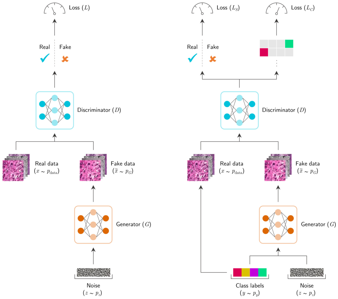
Traditional GAN struggles to generate high-resolution samples from highly variable data sets. This can be remedied by feeding the model with side information and forcing it to perform additional tasks. An auxiliary classifier GAN [54] builds upon the network structure of the standard GAN and adds data label information to both the generator and discriminator to improve the quality of the generated data and stabilize the training. Figure 1 showcases the key differences in design between the standard GAN and ACGAN.

In the ACGAN, every generated sample has a corresponding class label, $y\sim p_y$, in addition to the noise $\mathbf{z}$. The generator utilizes both to generate fake images. The discriminator receives a data sample as input and then outputs the probability distribution over sources, indicating the sample’s authenticity, as well as the probability distribution over the class labels. The objective function has two parts: the log-likelihood of the correct source, $L_S$, and the log-likelihood of the correct class, $L_C$.

$$L_S={\mathbb{E}}_{\mathbf{x}\sim p_{\mathrm{data}}}[log\left(D\left(\mathbf{x}\right)\right)]+{\mathbb{E}}_{\tilde{\mathbf{x}}\sim p_G}[1-log\left(D\left(\tilde{\mathbf{x}}\right)\right)]$$

(6)

$$L_C={\mathbb{E}}_{\mathbf{x}\sim p_{\mathrm{data}}}[logp\left(y|\mathbf{x}\right)]+{\mathbb{E}}_{\tilde{\mathbf{x}}\sim p_G}[logp\left(y_{\mathrm{fake}}|\tilde{\mathbf{x}}\right)]$$

(7)

where $y_{\mathrm{fake}}$ and $\tilde{\mathbf{x}}=G\left(\mathbf{z}|y_{\mathrm{fake}}\right)$ represent the category label of the generated sample and the generated sample, respectively, while $p\left(y|\mathbf{x}\right)$ and $p\left(y_{\mathrm{fake}}|\tilde{\mathbf{x}}\right)$ denote the correct classification probability for real and generated samples, respectively.

The total objective function combines the source adversarial loss and the auxiliary classification loss and is typically written as:

$$\underset{D}{max}\underset{G}{min}V\left(D,G\right)=[L_S\pm L_C]$$

(8)

The discriminator is trained to maximize both its ability to distinguish real samples from generated ones and its ability to accurately classify the images, which is achieved by optimizing the sum of both losses: ${max}_D\left(L_S+L_C\right)$. Conversely, the generator is trained to minimize the discriminator’s accuracy by encouraging it to accept generated samples as real and to classify them correctly. Because of this opposing goal, it minimizes the losses: ${min}_G\left(L_S-L_C\right)$. Hence, the joint optimization objective of an ACGAN, complemented with Wasserstein loss, can be summarized as:

$$\begin{array}{cc}\hfill \underset{D}{max}\underset{G}{min}V\left(D,G\right)& ={\mathbb{E}}_{\mathbf{x}\sim p_{\mathrm{data}}}\left[D\left(\mathbf{x}\right)\right]-{\mathbb{E}}_{\tilde{\mathbf{x}}\sim p_G}\left[D\left(\tilde{\mathbf{x}}\right)\right]\hfill \\ \hfill & \pm \left({\mathbb{E}}_{\mathbf{x}\sim p_{\mathrm{data}}}[logp\left(y|\mathbf{x}\right)]+{\mathbb{E}}_{\tilde{\mathbf{x}}\sim p_G}[logp\left(y_{\mathrm{fake}}|\tilde{\mathbf{x}}\right)]\right)\hfill \\ \hfill & -\lambda \mathbb{E}\left[{\left({∥\nabla D\left(\widehat{\mathbf{x}}\right)∥}_2-1\right)}^2\right]\hfill \end{array}$$

(9)

The ACGAN objective was constructed to encourage the generator to produce more class-discriminable samples while learning a representation for $\mathbf{z}$ that is independent of the class label.

4. Experimental Setup

4.1. Dataset Description

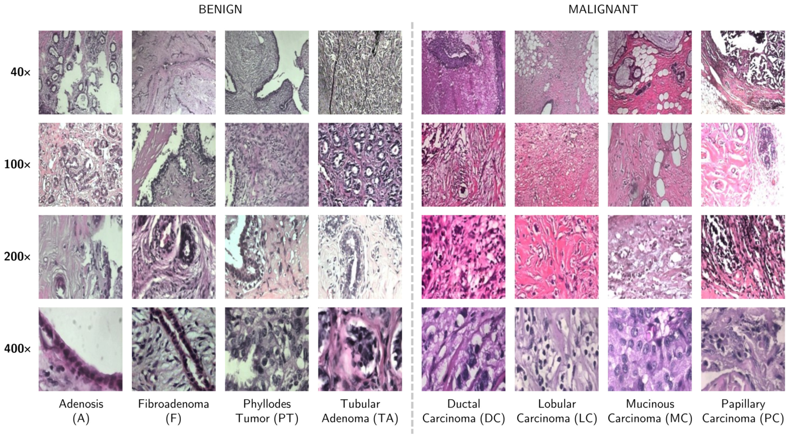
The Breast Cancer Histopathological Database (BreakHis) [55], used in this study, is an important resource for researchers focused on breast cancer classification. This publicly available dataset—collaboratively established with the P&D Laboratory of Pathological Anatomy and Cytopathology in Parana, Brazil—comprises 7909 microscopic images of breast tumor tissue, which are categorized into two primary classes: benign and malignant. The benign category encompasses a total of 2440 samples, while the malignant category contains 5429 samples in total. The samples have been obtained from a cohort of 82 patients, at different magnification levels of $40\times$, $100\times$, $200\times$, and $400\times$. The images are stored in .PNG format, with a resolution of $700\times 460$ pixels, and utilize a three-channel RGB color scheme. Notably, several example images are illustrated in Figure 2.

The BreakHis dataset comprehensively covers a spectrum of breast tumor subtypes, meticulously captured and annotated by expert pathologists. The benign tumor subtypes include: adenosis (A), fibroadenoma (F), phyllodes tumor (PT), and tubular adenoma (TA). The four featured malignant subtypes are ductal carcinoma (DC), lobular carcinoma (LC), mucinous carcinoma (MC), and papillary carcinoma (PC). Overall statistics regarding the dataset can be found in

Table 1. BreakHis data distribution.

Category	Subtype	Number of Patients	Magnification Level				Total
			$\mathbf{40}\times$	$\mathbf{100}\times$	$\mathbf{200}\times$	$\mathbf{400}\times$
Benign	A	4	114	113	111	106	444
	F	10	253	260	264	237	1014
	TA	3	109	121	108	115	453
	PT	7	149	150	140	130	569
Malignant	DC	38	864	903	896	788	3451
	LC	5	156	170	163	137	626
	MC	9	205	222	196	169	792
	PC	6	145	142	135	138	560
Total		82	1995	2081	2013	1820	7909

. This dataset serves as a strong foundation for training machine learning models, providing a diverse array of clinically relevant images that accurately represent the diagnostic challenges encountered in real-world scenarios.

4.2. Data Preparation

The images in the BreakHis dataset underwent a series of preprocessing steps, prior to feeding them to the ACGAN model, in an effort to facilitate model’s comprehension. The transformations included zero padding, median filtering, applying a contrast-limited adaptive histogram equalization (CLAHE) [56], and normalizing image pixels. By adding extra rows and columns filled with zeros around the image, thus extending it beyond its original boundaries, we attempted to ensure that edge pixels were handled effectively and that no critical information was lost at the image borders. To minimize additive noise and preserve the structural integrity of the tissue, a median filter was exerted. This non-linear filtering technique substitutes each pixel’s value with the median of its surrounding pixel values and, by doing so, eliminates the noise while keeping sharp edges. Given the uneven staining in histopathological images, CLAHE was used to increase local contrast and improve weak boundary detection. Dividing the image into small tiles, applying histogram equalization to each, and limiting the contrast to a specific threshold highlights critical features within the images, without over-amplifying noise or creating saturation. Subsequently, image pixels were normalized from $\left[0,255\right]$ to $\left[0,1\right]$, to advance model convergence during training. This standardization secures consistency in the input data distribution, which is paramount for optimizing the performance of deep learning models. Finally, the images were resized to a standard size, specifically $224\times 224$ pixels, to meet the compatibility requirements of the chosen pretrained models and ensure consistency.

During evaluation, 5-fold cross-validation is utilized to produce robust and reliable performance estimates and reduce the impact of data variability. This process involves partitioning the dataset randomly into five folds and then sequentially training and evaluating the model across multiple cycles. Each fold serves as the test set in turn, whereas the remaining four folds are combined to create a training set, ensuring the entire dataset is thoroughly engaged for both training and validation. The dataset is split in such a manner that in each iteration, 80% of the data is allocated for training and the residual 20% for testing. Stratified sampling is employed to preserve the original class distributions. To make sure the model generalizes well to new, previously unseen patients, we guarantee that the patient samples comprising a training set never overlap with those selected for testing. For binary classification, benign subtypes are grouped as the negative class, whilst in situ and invasive carcinomas are categorized as the positive class.

4.3. LSWACGAN Architecture

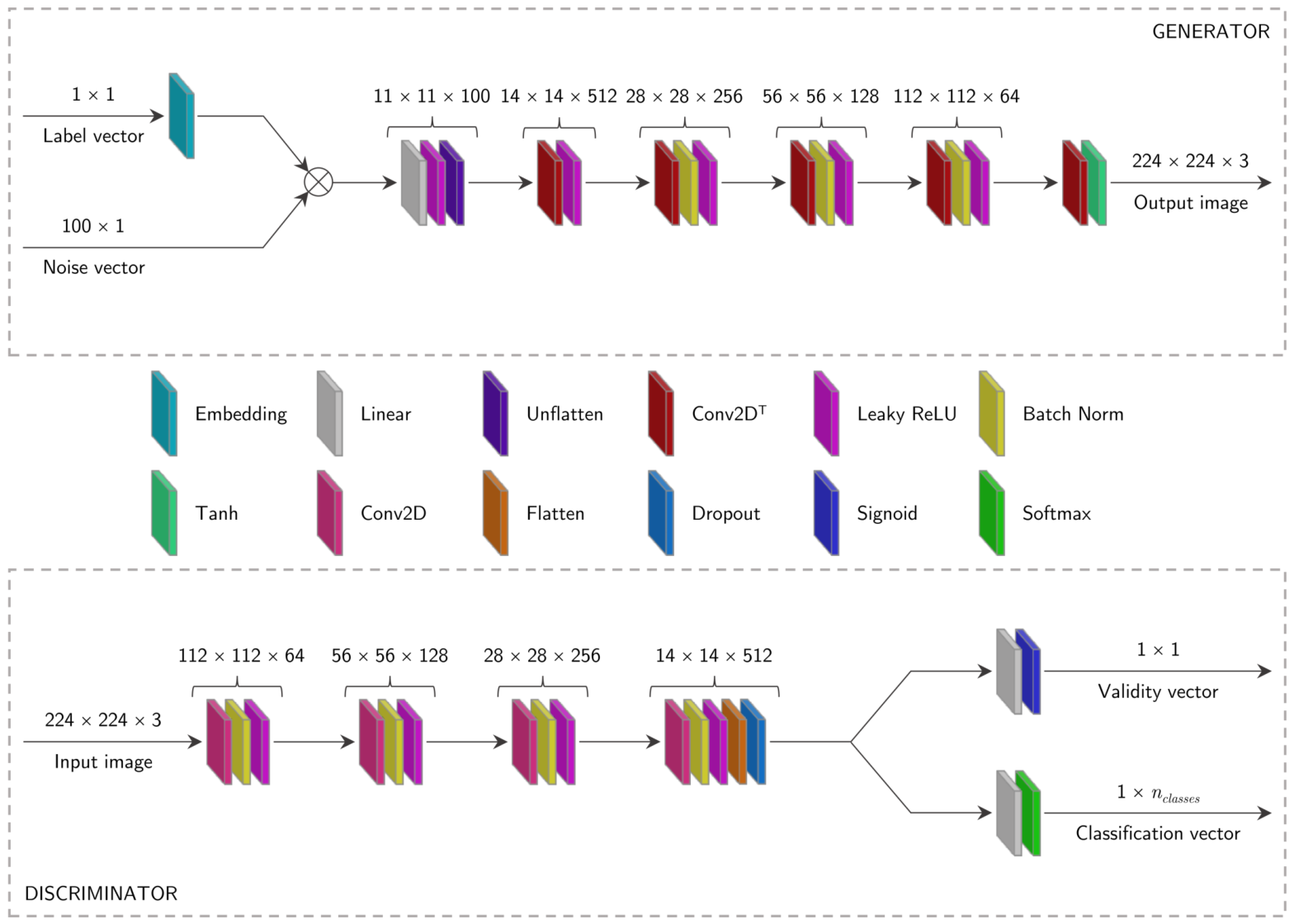
The generator receives a latent noise vector—sampled from a random normal distribution with a standard deviation of $0.2$—alongside a class label, and returns a single $224\times 224\times 3$ image. It boasts five transposed 2-d convolutional layers (${\mathrm{Conv}2\mathrm{D}}^{\mathrm{T}}$), containing $\{512,256,128,64,3\}$ filters, with a kernel of size $\left(4,4\right)$ and $\{1,2,2,2,2\}$ strides, respectively. The latent space dimension is fixed at 100. Initially, the class label is processed by an embedding layer—which converts it into an equivalent, continuous vector representation—and merged with the noise vector, indicating the point in latent space, through element-wise multiplication. Thus, the category information is fully integrated in the noise vector. Prior to running the sequence of ${\mathrm{Conv}2\mathrm{D}}^{\mathrm{T}}$ operations, the noise vector is passed through a fully-connected layer, comprising 12,100 nodes, to obtain activations that can be reshaped into a $\left(14,14,512\right)$ tensor. This transformation creates multiple low-resolution versions of the output image. All transpose convolutional layers in turn are followed by a batch normalization layer, ensuring that each input batch is normalized to have a zero mean and unit variance, and a Rectified Linear Unit (ReLU) activation layer—except the final one, which uses a hyperbolic tangent (tanh) activation function. In total, the generator encompasses approximately 4,798,580 trainable parameters.

The discriminator is a convolutional neural network architecture that takes in a single $224\times 224\times 3$ image and determines whether it is authentic or not, in addition to predicting its class label. The architecture comprises four blocks—each representing a 2-d convolutional layer (Conv2D), succeeded by a batch normalization layer and an activation layer—which include $\{64,128,256,512\}$ filters and a stride of $\left(2,2\right)$, respectively, in each layer. The activation function utilized in these blocks is Leaky ReLU [57], with a slope of $0.2$. Like the generator, the discriminator features $4\times 4$ filter kernels to expand the receptive field and enhance the expressive capability of the convolution. The output of the final block is flattened and forwarded through a dropout layer with a probability of $0.5$. After this, the network splits into two branches: one with sigmoid activation to distinguish real from fake images, and the other with softmax activation to produce the target class label. Both branches have a fully connected layer preceding their respective activations. The total number of trainable parameters for the discriminator is 3,660,681. The layered architecture of the proposed LSWACGAN is shown in Figure 3, while the more detailed description of the data flow and the dynamic interplay between the generator and the discriminator will be provided in the following subsections.

4.4. Label Smoothing and Label Flipping for Discriminator Training

To prevent the discriminator’s convergence speed from decreasing too rapidly, we implement several training tricks, including label smoothing and random label flipping. These techniques improve ACGAN stability and performance by reducing overfitting, particularly when training data are insufficient. Label smoothing involves replacing the “hard” labels of 1 for the correct class and 0 for all others—as in one-hot encoding—with softer targets, which can be represented as

$$y_i=\left\{\begin{array}{cc}1-\delta & i=\mathrm{correct}\\ {\displaystyle \frac{\delta }{N-1}}& i=\mathrm{others}\end{array}\right.$$

(10)

where $\delta$ is a hyperparameter and N represents the total number of classes. By smoothing the labels, the generator is discouraged from producing fake images with absolute confidence, while the discriminator avoids becoming overly certain in its predictions, leading to improved generalization and robustness.

Another way to criple the discriminator is to introduce label noise by randomly flipping a portion of labels assigned to both real and fake images during training. In doing so, the discriminator is deliberately misled to believe that some real images are actually synthesized by the generator; thus making its classification task more difficult. This added element of randomness enhances the discriminator’s resilience to imperfections during inference, resulting in better performance on unseen data.

4.5. Training Strategy

During training, the generator and discriminator networks are updated alternatively, in an adversarial manner. The generator adapts its weights to better replicate the distribution of the target data. Meanwhile, the discriminator also continuously adjusts its weights, thereby enhancing its own ability to accurately classify images and effectively determine whether they are real or synthetic. The training process encompasses several key steps: (i) generating pseudo-images, (ii) optimizing the discriminator, and (iii) optimizing the generator via the discriminator. Initially, m random n-dimensional tensors—where m denotes the batch size—along with their randomly spruced labels, are fed into the generator network. Upon processing them, the generator outputs data, matching the shape and size of the real images, that represent pseudo-images. These pseudo-images, combined with the equally sized batch of real images, are then input into the discriminator network. The discriminator aims to determine whether each input is a real or a pseudo-image and to classify it correctly. The discriminator network parameters are optimized using the corresponding validation loss, classification loss, and the gradient penalty term. After optimizing its parameters, a new batch of generated pseudo-images is again passed through a discriminator, which verifies their authenticity. With the discriminator network parameters held constant, the generator network parameters are subsequently optimized based on the classification loss and validation loss. A detailed training strategy is presented in Algorithm 1.

Algorithm 1 Training procedure of the proposed LSWACGAN model

Initialize discriminator D and generator G Define parameters: number of epochs $n\_epochs$, number of batches $n\_batch$, batch size m, Adam hyperparameter $\alpha$, ${\beta }_1$, ${\beta }_2$, gradient penalty coefficient $\lambda$, random number $ϵ$ from uniform distribution $[0,1]$ for each epoch in $\left(1,\dots ,n\_epochs\right)$ do       for each batch in $\left(1,\dots ,n\_batch\right)$ do             Sample m random vectors $\mathbf{z}$ with labels y             Generate a batch of fake images: $\tilde{\mathbf{X}}\leftarrow \left\{G\left({\mathbf{z}}^{\left(1\right)},y^{\left(1\right)}\right),\dots ,G\left({\mathbf{z}}^{\left(m\right)},y^{\left(m\right)}\right)\right\}$             Sample a batch of m real images: $\mathbf{X}\leftarrow \left\{{\mathbf{x}}^{\left(1\right)},\dots ,{\mathbf{x}}^{\left(m\right)}\right\}$             Perform one-sided smoothing of real data labels             Input real images $\left(\mathbf{X}\right)$ into the discriminator             Input fake images $\left(\tilde{\mathbf{X}}\right)$ into the discriminator             Compute validation loss ${\mathcal{L}}_S^{\left(i\right)}\leftarrow {\displaystyle \frac{1}{m}}\sum D\left(\tilde{\mathbf{X}}\right)-{\displaystyle \frac{1}{m}}\sum D\left(\mathbf{X}\right)$             Compute classification loss ${\mathcal{L}}_C^{\left(i\right)}$ according to the CE loss function definition             Randomly mix real and fake images: $\widehat{\mathbf{X}}\leftarrow ϵ\mathbf{X}+\left(1-ϵ\right)\tilde{\mathbf{X}}$             Calculate total discriminator loss ${\mathcal{L}}_D^{\left(i\right)}\leftarrow {\mathcal{L}}_S^{\left(i\right)}-{\mathcal{L}}_C^{\left(i\right)}+{\displaystyle \frac{1}{m}}\sum \lambda {\left({∥{\nabla }_{\widehat{\mathbf{X}}}D\left(\widehat{\mathbf{X}}\right)∥}_2-1\right)}^2$             Update discriminator weights using backpropagation with Adam             Sample another m random vectors $\mathbf{z}$ with labels y             Generate new batch of fake images: $\tilde{\mathbf{X}}\leftarrow \left\{G\left({\mathbf{z}}^{\left(1\right)},y^{\left(1\right)}\right),\dots ,G\left({\mathbf{z}}^{\left(m\right)},y^{\left(m\right)}\right)\right\}$             Input fake images $\left(\tilde{\mathbf{X}}\right)$ into the discriminator             Compute validation loss ${\mathcal{L}}_S^{\left(i\right)}\leftarrow -{\displaystyle \frac{1}{m}}\sum D\left(\tilde{\mathbf{X}}\right)$             Compute classification loss ${\mathcal{L}}_C^{\left(i\right)}$ according to the CE loss function definition             Calculate total generator loss ${\mathcal{L}}_G^{\left(i\right)}\leftarrow {\mathcal{L}}_S^{\left(i\right)}-{\mathcal{L}}_C^{\left(i\right)}$             Update generator weights using backpropagation with Adam       end for end for

The parametric updates ${\theta }_d$ and ${\theta }_g$ are carried out by training the proposed ACGAN architecture for 2000 epochs, utilizing a batch size $m=64$. In each epoch, the images are first randomly shuffled, then input into the model batch by batch. A random undersampling technique is applied to effectively neutralize class imbalance, ensuring that all classes are adequately represented during training. Adam—with a learning rate of $2\times {10}^{-4}$ and the momentum $\beta$ set to $0.5$—is employed as the optimizer of choice due to its efficacy in handling of sparse gradients, minimal memory requirements, and strong computational performance. The structure of the networks, hyperparameter values, and the optimization algorithm have been carefully tuned through several iterations of the model selection process to ensure network stability, smooth convergence, and to avoid mode collapse.

All code was implemented utilizing PyTorch version 2.10.0 with CUDA 12.8. Experiments were executed in a cloud-based Google Colab environment, which offers complimentary access to computing resources, including GPUs and TPUs. The current setup includes an NVIDIA Tesla T4 GPU, equipped with 40 streaming multiprocessors, 6 MB L2 cache shared across the system, and 16 GB of high-bandwidth GDDR6 RAM. Pre-installed Python 3.x packages further support efficient computations.

5. Results and Discussion

The proposed LSWACGAN’s efficacy for data-efficient breast tumor classification was evaluated by turning its discriminator into a classifier after training and assessing its performance across several key metrics: accuracy, precision, recall (also known as sensitivity), specificity, and F1-score. Precision shows how well the classifier avoids falsely labelling negative samples as positive. Recall measures how well it identifies all individuals affected by the disease, reflecting the true-positive rate. The F1-score blends precision and recall into a single measure by taking their weighted average. Specificity highlights the classifier’s ability to correctly spot those individuals free from the disease, representing the true-negative rate. These metrics together provide a comprehensive appraisal of the classifier’s strengths in distinguishing between positive and negative cases.

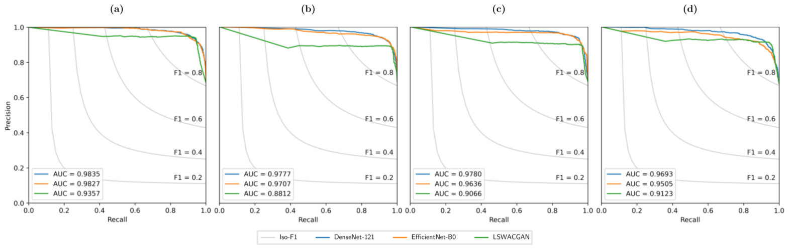
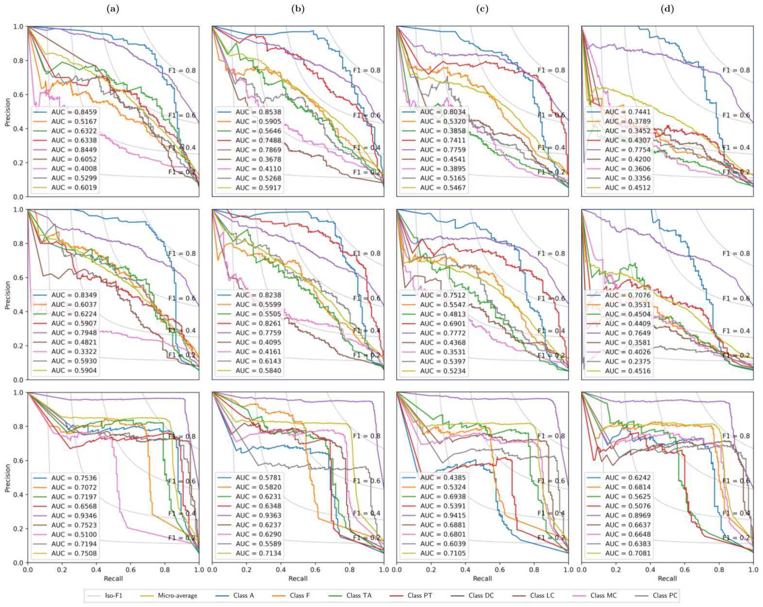
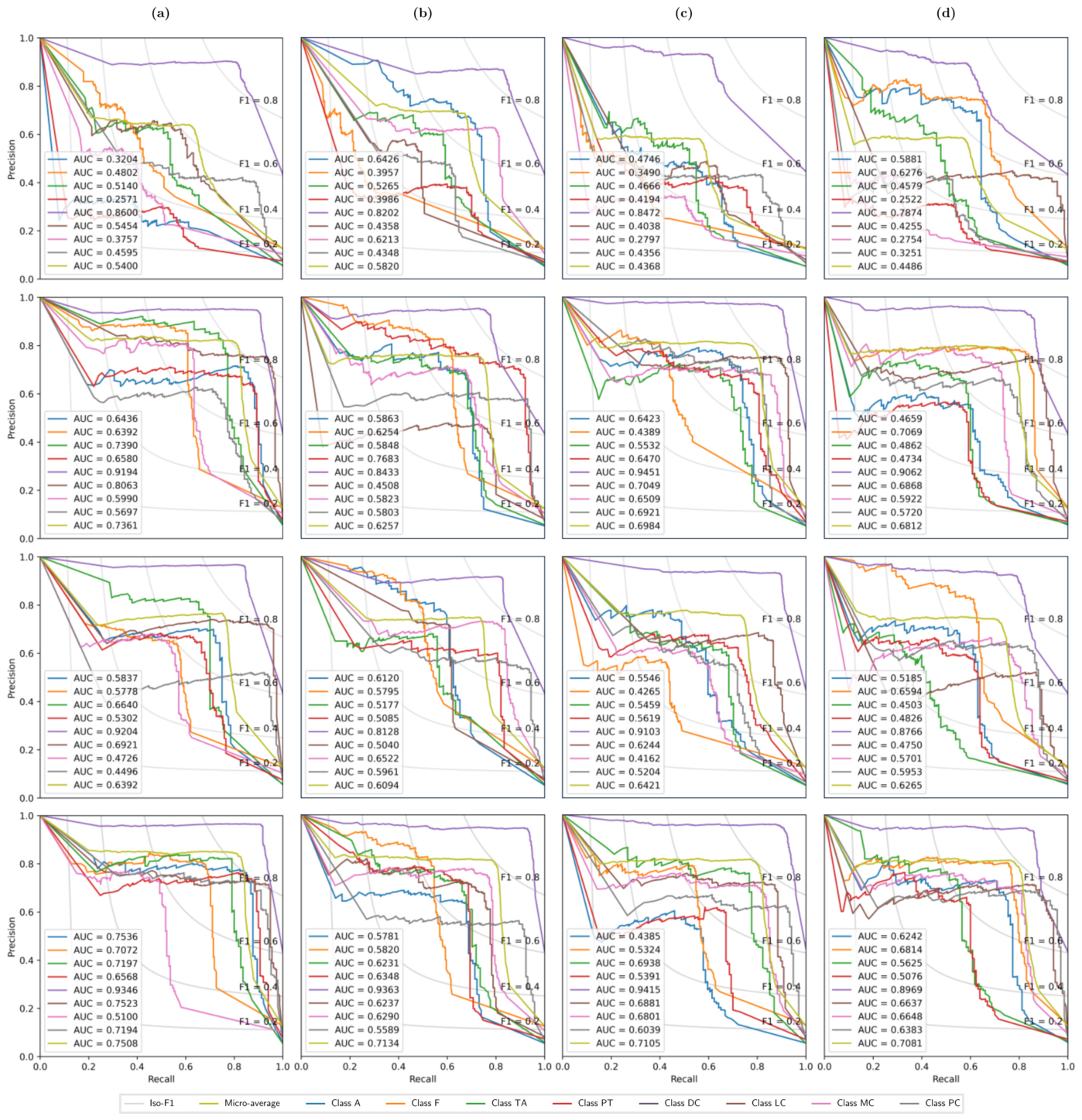
Due to the noticeable class imbalance in the experimental data, we opted to use precision–recall (P-R) curves rather than Receiver Operating Characteristic (ROC) curves, as the former tend to provide more valuable insights than the latter in such imbalanced scenarios [58]. A P-R curve is constructed by plotting precision and recall at various probability thresholds. Furthermore, Iso-F1 curves—which represent points with equal F1 scores—are overlaid on the P-R curves to facilitate performance evaluation. A quantitative performance metric, the Area Under the Curve (AUC), is also calculated for each target class and displayed alongside the average AUC on all the plots. Unlike single-threshold-based metrics, PR-AUC measures how the model performs across all possible thresholds. It captures the overall relationship between true positives and false positives; in other words, it shows how well the model separates “good” from “bad” cases, no matter where you draw the line. The higher the PR-AUC score, the better the classifier. Compared to ROC-AUC, PR-AUC focuses on the precision–recall trade-off and is thus not prone to overly optimistic evaluations when one class is dominant, providing a more honest and rigorous evaluation of the classifier’s skill.

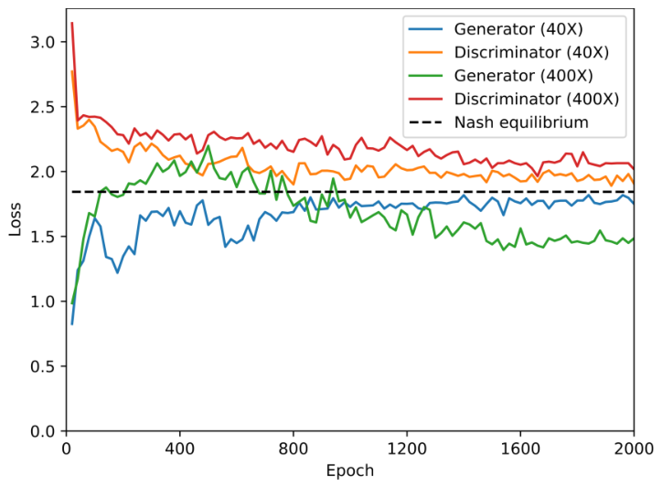
Furthermore, the proposed LSWACGAN training loss in a multi-class scenario has been thoroughly analyzed to uncover how the network converges. Figure 4 shows source losses—representing real and fake samples—for both the generator and discriminator at the lowest $(40\times )$ and the highest $(400\times )$ magnification levels. For clarity purposes, loss values were recorded every 20 epochs. From the figure, it is evident that the network reaches a value close to the Nash equilibrium after approximately 1500 epochs. Training at $40\times$ magnification demonstrates a relatively smooth trajectory towards the equilibrium. In contrast, the highest magnification results in a slightly deviated convergence from the equilibrium value. These findings suggest that the network effectively captures the underlying factors driving variation across classes in the training distribution, which helps it generalize better to new data. Consistent convergence within the designated number of epochs is also observed when the network is trained on images acquired at the other two standard magnification levels.

5.1. Model Comparison

To experimentally verify that the proposed LSWACGAN is advantageous, we benchmark it against two cutting-edge convolutional neural network architectures: DenseNet-121 [59] and EfficientNet-B0 [60]. DenseNet and EfficientNet currently mark the state of the art in computer vision because they effectively address the trade-off between accuracy and computational efficiency. They achieve superior performance—specifically, high accuracy on datasets like ImageNet—while using significantly fewer parameters and lower computational cost (FLOPs) than traditional architectures like VGG or ResNet.

Due to the limited quantity and characteristics of our training data, transfer learning is employed to maximize the potential of DenseNet-121 and EfficientNet-B0 by using pretrained weights from ImageNet. This widely adopted approach leverages the existing features and model parameters to boost performance on a new task, reducing training time and improving classification accuracy. Fine-tuning is further applied to adapt the pretrained models to the specific application of identifying breast tumor manifestations in histopathological images, through a two-stage process. First, both pretrained models had their final layers beyond the last activation layer swapped for custom-designed heads tailored to each architecture. For EfficientNet-B0, the new head comprises a dropout layer with a $0.2$ dropout rate, followed by a single fully connected layer, providing regularization directly before the output. DenseNet-121’s new head is a bit more complex, featuring a fully connected layer, a ReLU activation layer, a dropout layer with a probability of $0.5$ for stronger regularization, and a second fully connected layer prior to the output. In both cases, a softmax activation is added at the end to support binary or multi-class classification. Subsequently, all model parameters were unfrozen and retrained from scratch for 10 epochs, utilizing the same learning rate and Adam optimizer as in our proposed LSWACGAN to ensure a fair comparison.

Table 2. Performance measures for binary model comparison.

		Accuracy		Precision		Recall
Magnification	Model	Mean	95% CI	Mean	95% CI	Mean	95% CI
$40\times$	DenseNet-121	0.9043	0.8646, 0.9439	0.9377	0.8818, 0.9936	0.9248	0.8745, 0.9751
	EfficientNet-B0	0.8922	0.8543, 0.9301	0.9396	0.8946, 0.9846	0.9022	0.8698, 0.9346
	LSWACGAN	0.9218	0.8806, 0.9630	0.9456	0.9061, 0.9851	0.9409	0.9088, 0.9730
		Specificity		F1-score		PR-AUC
	Model	Mean	95% CI	Mean	95% CI	Mean	95% CI
	DenseNet-121	0.8592	0.7150, 1.000	0.9300	0.9023, 0.9577	0.9835	0.9673, 0.9997
	EfficientNet-B0	0.8704	0.7688, 0.9720	0.9201	0.8925, 0.9477	0.9827	0.9670, 0.9985
	LSWACGAN	0.8800	0.7909, 0.9691	0.9430	0.9133, 0.9727	0.9357	0.8562, 1.0000
		Accuracy		Precision		Recall
Magnification	Model	Mean	95% CI	Mean	95% CI	Mean	95% CI
$100\times$	DenseNet-121	0.9025	0.8613, 0.9436	0.9193	0.8607, 0.9780	0.9444	0.9138, 0.9749
	EfficientNet-B0	0.9020	0.8460, 0.9579	0.9243	0.8587, 0.9900	0.9374	0.9116, 0.9632
	LSWACGAN	0.8948	0.8505, 0.9390	0.8934	0.8350, 0.9519	0.9659	0.9269, 1.0000
		Specificity		F1-score		PR-AUC
	Model	Mean	95% CI	Mean	95% CI	Mean	95% CI
	DenseNet-121	0.8088	0.6555, 0.9621	0.9308	0.9035, 0.9581	0.9777	0.9605, 0.9949
	EfficientNet-B0	0.8227	0.6579, 0.9875	0.9302	0.8924, 0.9679	0.9707	0.9413, 1.0000
	LSWACGAN	0.7362	0.5694, 0.9030	0.9272	0.8985, 0.9559	0.8812	0.8033, 0.9591
		Accuracy		Precision		Recall
Magnification	Model	Mean	95% CI	Mean	95% CI	Mean	95% CI
$200\times$	DenseNet-121	0.9140	0.8511, 0.9769	0.9417	0.8901, 0.9933	0.9345	0.8720, 0.9971
	EfficientNet-B0	0.9016	0.8403, 0.9629	0.9408	0.8688, 1.0000	0.9194	0.8506, 0.9883
	LSWACGAN	0.9002	0.8606, 0.9398	0.8987	0.8627, 0.9346	0.9647	0.9435, 0.9860
		Specificity		F1-score		PR-AUC
	Model	Mean	95% CI	Mean	95% CI	Mean	95% CI
	DenseNet-121	0.8681	0.7457, 0.9905	0.9374	0.8917, 0.9830	0.9780	0.9465, 1.0000
	EfficientNet-B0	0.8615	0.6806, 1.0000	0.9281	0.8840, 0.9723	0.9636	0.8955, 1.0000
	LSWACGAN	0.7561	0.6640, 0.8481	0.9304	0.9034, 0.9574	0.9066	0.8533, 0.9600
		Accuracy		Precision		Recall
Magnification	Model	Mean	95% CI	Mean	95% CI	Mean	95% CI
$400\times$	DenseNet-121	0.8742	0.7955, 0.9529	0.9336	0.8723, 0.9950	0.8790	0.7710, 0.9871
	EfficientNet-B0	0.8593	0.7746, 0.9440	0.9015	0.8326, 0.9703	0.8936	0.7786, 1.0000
	LSWACGAN	0.9104	0.8806, 0.9402	0.9137	0.9003, 0.9270	0.9585	0.9044, 1.0000
		Specificity		F1-score		PR-AUC
	Model	Mean	95% CI	Mean	95% CI	Mean	95% CI
	DenseNet-121	0.8636	0.7256, 1.0000	0.9031	0.8374, 0.9687	0.9693	0.9403, 0.9982
	EfficientNet-B0	0.7869	0.6131, 0.9608	0.8945	0.8261, 0.9629	0.9505	0.9005, 1.0000
	LSWACGAN	0.8094	0.7701, 0.8488	0.9351	0.9111, 0.9590	0.9123	0.8799, 0.9448

Boldface indicates the highest value for each metric across all models. Underlining denotes the best metric scores for each model.

and

Table 3. Performance measures for multi-class model comparison.

		Accuracy		Precision		Recall
Magnification	Model	Mean	95% CI	Mean	95% CI	Mean	95% CI
$40\times$	DenseNet-121	0.5840	0.5120, 0.6560	0.5648	0.4880, 0.6416	0.6110	0.4825, 0.7396
	EfficientNet-B0	0.5649	0.4944, 0.6354	0.5489	0.4908, 0.6069	0.5912	0.4786, 0.7039
	LSWACGAN	0.8401	0.7699, 0.9103	0.7845	0.6816, 0.8874	0.8213	0.7586, 0.8841
		Specificity		F1-score		PR-AUC
	Model	Mean	95% CI	Mean	95% CI	Mean	95% CI
	DenseNet-121	0.9391	0.9299, 0.9483	0.5523	0.4554, 0.6492	0.6019	0.5136, 0.6903
	EfficientNet-B0	0.9351	0.9252, 0.9450	0.5385	0.4557, 0.6214	0.5904	0.4656, 0.7153
	LSWACGAN	0.9769	0.9668, 0.9871	0.7778	0.6733, 0.8823	0.7508	0.6410, 0.8607
		Accuracy		Precision		Recall
Magnification	Model	Mean	95% CI	Mean	95% CI	Mean	95% CI
$100\times$	DenseNet-121	0.5695	0.5159, 0.6231	0.5571	0.4788, 0.6355	0.5651	0.4637, 0.6666
	EfficientNet-B0	0.5574	0.4974, 0.6175	0.5535	0.4319, 0.6751	0.6009	0.4691, 0.7327
	LSWACGAN	0.8121	0.7211, 0.9031	0.7668	0.6450, 0.8885	0.7526	0.6151, 0.8901
		Specificity		F1-score		PR-AUC
	Model	Mean	95% CI	Mean	95% CI	Mean	95% CI
	DenseNet-121	0.9339	0.9274, 0.9405	0.5353	0.4485, 0.6221	0.5917	0.5099, 0.6736
	EfficientNet-B0	0.9338	0.9265, 0.9411	0.5501	0.4298, 0.6703	0.5840	0.4797, 0.6884
	LSWACGAN	0.9723	0.9600, 0.9846	0.7204	0.5685, 0.8722	0.7134	0.5759, 0.8510
		Accuracy		Precision		Recall
Magnification	Model	Mean	95% CI	Mean	95% CI	Mean	95% CI
$200\times$	DenseNet-121	0.5714	0.4805, 0.6623	0.5369	0.4575, 0.6164	0.5778	0.4875, 0.6682
	EfficientNet-B0	0.5495	0.4679, 0.6311	0.5294	0.4552, 0.6035	0.5739	0.4718, 0.6759
	LSWACGAN	0.8182	0.7745, 0.8619	0.7197	0.6651, 0.7743	0.7695	0.7113, 0.8278
		Specificity		F1-score		PR-AUC
	Model	Mean	95% CI	Mean	95% CI	Mean	95% CI
	DenseNet-121	0.9358	0.9222, 0.9494	0.5208	0.4454, 0.5961	0.5467	0.3874, 0.7060
	EfficientNet-B0	0.9334	0.9207, 0.9462	0.5182	0.4363, 0.6001	0.5234	0.3839, 0.6630
	LSWACGAN	0.9737	0.9672, 0.9802	0.7260	0.6738, 0.7783	0.7105	0.6658, 0.7552
		Accuracy		Precision		Recall
Magnification	Model	Mean	95% CI	Mean	95% CI	Mean	95% CI
$400\times$	DenseNet-121	0.4786	0.3670, 0.5901	0.4398	0.3223, 0.5574	0.4819	0.4139, 0.5500
	EfficientNet-B0	0.4758	0.3735, 0.5782	0.4435	0.3646, 0.5225	0.4671	0.4016, 0.5326
	LSWACGAN	0.8115	0.7310, 0.8921	0.7646	0.6662, 0.8630	0.7791	0.7055, 0.8527
		Specificity		F1-score		PR-AUC
	Model	Mean	95% CI	Mean	95% CI	Mean	95% CI
	DenseNet-121	0.9247	0.9082, 0.9412	0.4114	0.3599, 0.4629	0.4512	0.3011, 0.6014
	EfficientNet-B0	0.9223	0.9068, 0.9377	0.4181	0.3662, 0.4701	0.4516	0.3346, 0.5686
	LSWACGAN	0.9723	0.9627, 0.9818	0.7415	0.6483, 0.8348	0.7081	0.5765, 0.8396

Boldface indicates the highest value for each metric across all models. Underlining denotes the best metric scores for each model.

summarize the performance of the proposed LSWACGAN classifier, alongside two selected supervised baseline models, covering both binary and multi-class scenarios. The results showcase all specified evaluation metrics across various magnification levels. For each metric, the highest value within each model is underlined, while the overall top values across all models are displayed in bold, to emphasize the key points of comparison.

The experimental results indicate that in both scenarios, the best overall performance is achieved on the $40\times$ dataset compared with other magnifications. One possible reason is that the $40\times$ magnification reveals more distinct cancerous patterns that may not be visible at higher magnification, thus enabling a broader, more comprehensive overview of tissue architecture. In the binary classification scenario, LSWACGAN closely matches or slightly exceeds its rivals across most metrics. This advantage is most noticeable in recall rates, where LSWACGAN surpasses DenseNet-121 by $1.61\%$, $2.15\%$, $3.07\%$, and $7.95\%$ and outperforms EfficientNet-B0 by $3.87\%$, $2.85\%$, $4.53\%$, and $6.49\%$, respectively, on the corresponding datasets. Maximizing recall (or sensitivity) is prioritized in medical diagnosis—even if it means settling for lower precision as a trade-off—since the cost of missing a critical diagnosis is far greater than that of a mistaken one, which can be eventually cleared by follow-up tests.

In the multi-class scenario, LSWACGAN emerges as the clear favorite, delivering superior results across all evaluation metrics and magnification levels, whilst DenseNet-121 and EfficientNet-B0—despite their strengths—struggle and lag behind performance-wise. Although the binary scenario reaches a peak classification accuracy of $92.18\%$, the multi-class scenario yields the largest differences in evaluation metrics, compared to baseline models. This further substantiates LSWACGAN’s commendable data efficiency and ability to produce competitive results with minuscule training data, comprising fewer than 1000 samples per class. The most significant improvements with LSWACGAN between the two scenarios occur in specificity. This stems from the fact that multi-class classifiers focus on maximizing the margin between all classes simultaneously, which in turn leads to more robust, tighter, and less “false-positive-prone” boundaries for each class. Moreover, it is worth noting that LSWACGAN maintains fairly consistent performance at varying magnification levels, whereas its state-of-the-art competitors experience severe performance degradation as magnification increases. This can be attributed to modifications implemented in the ACGAN architecture and learning strategy, which boost mathematical stability during training, enabling LSWACGAN to more effectively bridge the gap between lower- and higher-resolution data.

Although the proposed LSWACGAN classifier yields acceptable success rates, even at higher magnification levels, its predictive reliability should also be examined. Therefore, $95\%$ confidence intervals are calculated for each metric and are presented in Table 2 and Table 3. In a k-fold validation setup, the confidence interval is defined as:

$$CI=\overline{x}\pm t^{*}·\left({\displaystyle \frac{s}{k}}\right)$$

(11)

where $\overline{x}$ represents the sample mean, s is the standard deviation, and $t^{*}$ is the critical value from the standard t-distribution. A $95\%$ confidence interval does not guarantee that the true value will fall within the calculated interval for any single sample. Instead, it means that if the sampling process was repeated many times, about $95\%$ of those intervals would contain the true value. Rather than relying on a single point estimate, confidence intervals provide a likely range for the true value, offering a clearer picture of fidelity and uncertainty. The tables show that the confidence intervals for the LSWACGAN classifier are generally narrower than those of the baseline—particularly, in the multi-class scenario—indicating reduced variability in confidence across metrics and making it a reliable candidate for high-stakes, decision-critical applications.

To gain a more nuanced perspective on the classifier performance, the corresponding P-R curves for the binary and multi-class scenarios are plotted in Figure 5 and Figure 6. Along with notable differences in accuracy across magnification levels in both binary and multi-class scenarios, the P-R curves for the same exhibit equivalent trends. In addition, the P-R performance in the binary scenario is remarkably better than that in the multi-class scenario for all magnification levels, which is in harmony with other results provided in Table 2 and Table 3. It is quite interesting to point out that in the binary scenario, the proposed LSWACGAN yields lower PR-AUC values than the baseline models, though its classification accuracy and recall match or even slightly surpass theirs for most magnification levels. This occurs because PR-AUC evaluates the performance across all possible classification thresholds, whereas other metrics report values at a single default threshold of $0.5$. Minor threshold shifts, leading to lower precision, can degrade the PR-AUC score, even if performance at the main operating point is strong. In the multi-class scenario, the LSWACGAN’s performance, shown in the bottom panel, well exceeds that of its competitors for most classes, with this gap widening as magnification increases. The drop in performance at lower magnification levels is mainly due to classes (subtypes) A, F, MC, and PC, while classes (subtypes) TA and PF have a more exuberant effect at higher magnifications.

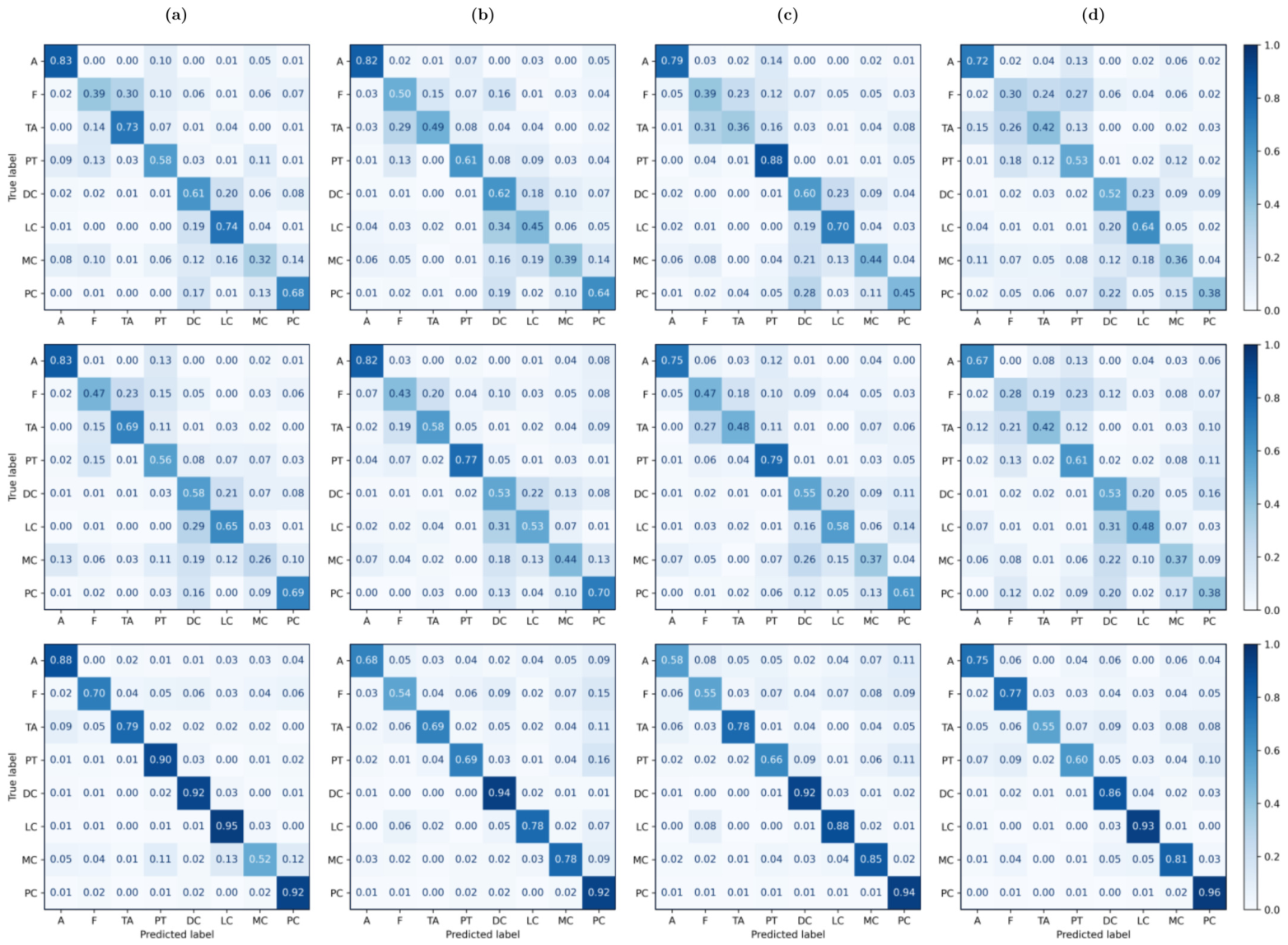
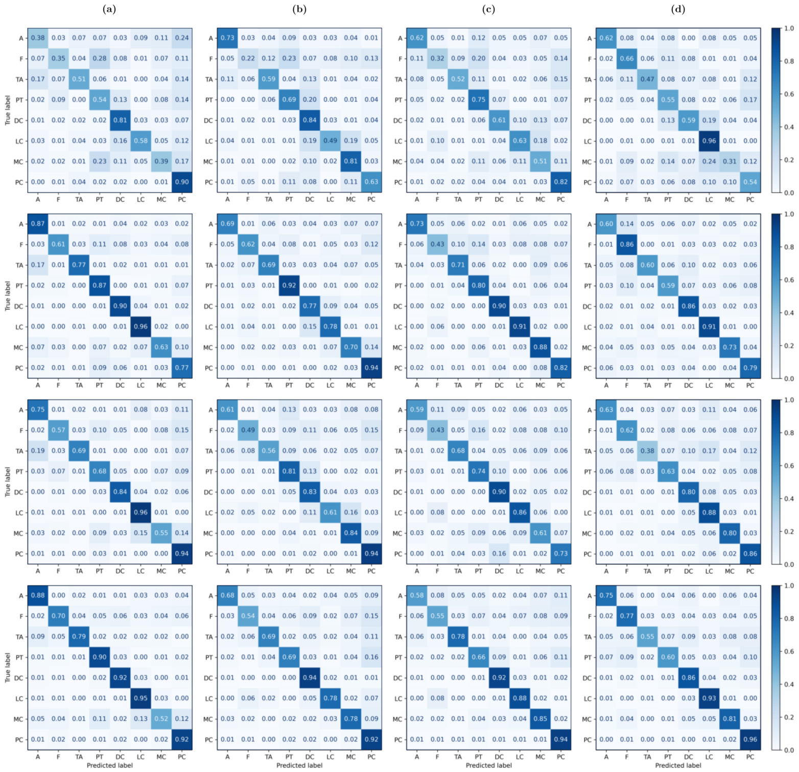
With the aim of deepening our grasp of classifier uncertainty across different classes, Figure 7 illustrates confusion matrices for the proposed LSWACGAN, along with those for the two selected baseline models, in the multi-class scenario. Vis-à-vis the baselines, the proposed LSWACGAN exhibits a significantly reduced degree of uncertainty. All models, as anticipated, struggle more when transitioning from lower to higher magnification levels. Notably, for both baselines, confusion for class (subtype) A is always among the lowest of all classes (subtypes), despite it being the least-represented class (subtype) in the experimental data. This rather surprising phenomenon arises because convolutional neural networks tend to latch onto a few highly specific, low-diversity features. While the majority of classes require a broader, more varied decision space, convolutional neural networks can effectively recognize minority classes using only a handful of distinct features. On the other hand, the generative model behind the proposed classifier delivers steadier results, less swayed by class imbalance in the training dataset.

5.2. Ablation Study

Ablation is a procedure with a long history in neuroscience, where controlled damage is introduced into neural tissue to investigate how injuries affect the brain’s ability to perform assigned tasks. In recent years, this technique has inspired a widely used, but broadly defined, methodology for validating and interpreting deep learning models. In this context, ablation studies systematically deactivate or eliminate model components to analyze each component’s influence on overall system functionality and identify which parts of a model contribute most to its performance (e.g., separating “weaker learners” from essential ones). For ablation to be effective, the system must exhibit slow degradation, continuing to function despite missing specific components, so that the value of each removed part can be clearly measured by comparison with the full model. As we are interested in understanding the reasons behind the performance improvement of the proposed semi-supervised LSWACGAN classifier—a crucial step for further boosting its transparency and efficiency in the future—we thoroughly examine the impact of ablating key components to gauge their importance. The selected combinations comprise the standard ACGAN, the Wasserstein ACGAN (WACGAN), and the label-smoothed ACGAN (LSACGAN). To guarantee a fair and bias-free comparison, all variants were trained and evaluated under identical experimental conditions, including the same preprocessing pipeline, dataset splits, and training strategy.

Table 4. Performance measures for binary ablation study.

		Accuracy		Precision		Recall
Magnification	Model	Mean	95% CI	Mean	95% CI	Mean	95% CI
$40\times$	ACGAN	0.8371	0.7960, 0.8782	0.8726	0.7966, 0.9485	0.9015	0.8200, 0.9830
	WACGAN	0.9208	0.8709, 0.9707	0.9403	0.8840, 0.9966	0.9467	0.9025, 0.9909
	LSACGAN	0.8932	0.8330, 0.9534	0.9108	0.8222, 0.9995	0.9431	0.8965, 0.9897
	LSWACGAN	0.9218	0.8806, 0.9630	0.9456	0.9061, 0.9851	0.9409	0.9088, 0.9730
		Specificity		F1-score		PR-AUC
	Model	Mean	95% CI	Mean	95% CI	Mean	95% CI
	ACGAN	0.6960	0.4810, 0.9110	0.8837	0.8556, 0.9118	0.9012	0.8391, 0.9633
	WACGAN	0.8640	0.7295, 0.9985	0.9428	0.9072, 0.9784	0.9363	0.8619, 1.0000
	LSACGAN	0.7840	0.5623, 1.0000	0.9247	0.8849, 0.9645	0.9128	0.8288, 0.9967
	LSWACGAN	0.8800	0.7909, 0.9691	0.9430	0.9133, 0.9727	0.9357	0.8562, 1.0000
		Accuracy		Precision		Recall
Magnification	Model	Mean	95% CI	Mean	95% CI	Mean	95% CI
$100\times$	ACGAN	0.8630	0.7878, 0.9382	0.8871	0.8159, 0.9584	0.9227	0.8328, 1.000
	WACGAN	0.9116	0.8753, 0.9478	0.9306	0.8611, 1.0000	0.9471	0.8972, 0.9970
	LSACGAN	0.8708	0.8317, 0.9098	0.8977	0.7980, 0.9974	0.9326	0.8089, 1.0000
	LSWACGAN	0.8948	0.8505, 0.9390	0.8934	0.8350, 0.9519	0.9659	0.9269, 1.0000
		Specificity		F1-score		PR-AUC
	Model	Mean	95% CI	Mean	95% CI	Mean	95% CI
	ACGAN	0.7298	0.5387, 0.9208	0.9026	0.8463, 0.9588	0.9166	0.8435, 0.9898
	WACGAN	0.8323	0.6555, 1.0000	0.9370	0.9136, 0.9604	0.9287	0.8612, 0.9963
	LSACGAN	0.7327	0.4614, 1.0000	0.9080	0.8747, 0.9412	0.8666	0.7440, 0.9893
	LSWACGAN	0.7362	0.5694, 0.9030	0.9272	0.8985, 0.9559	0.8812	0.8033, 0.9591
		Accuracy		Precision		Recall
Magnification	Model	Mean	95% CI	Mean	95% CI	Mean	95% CI
$200\times$	ACGAN	0.8490	0.7789, 0.9191	0.9065	0.8171, 0.9958	0.8842	0.7282, 1.000
	WACGAN	0.9121	0.8631, 0.9610	0.9156	0.8745, 0.9566	0.9626	0.9028, 1.0000
	LSACGAN	0.8912	0.8593, 0.9230	0.9023	0.8414, 0.9632	0.9496	0.8832, 1.0000
	LSWACGAN	0.9002	0.8606, 0.9398	0.8987	0.8627, 0.9346	0.9647	0.9435, 0.9860
		Specificity		F1-score		PR-AUC
	Model	Mean	95% CI	Mean	95% CI	Mean	95% CI
	ACGAN	0.7699	0.5330, 1.0000	0.8869	0.8207, 0.9531	0.8981	0.7789, 1.0000
	WACGAN	0.7991	0.6894, 0.9088	0.9377	0.9018, 0.9737	0.9147	0.8275, 1.0000
	LSACGAN	0.7604	0.5931, 0.9278	0.9234	0.9013, 0.9455	0.9167	0.8274, 1.0000
	LSWACGAN	0.7561	0.664, 0.8481	0.9304	0.9034, 0.9574	0.9066	0.8533, 0.9600
		Accuracy		Precision		Recall
Magnification	Model	Mean	95% CI	Mean	95% CI	Mean	95% CI
$400\times$	ACGAN	0.8280	0.7079, 0.9482	0.8913	0.8519, 0.9307	0.8508	0.6532, 1.0000
	WACGAN	0.8879	0.8502, 0.9256	0.9245	0.8707, 0.9783	0.9139	0.8076, 1.0000
	LSACGAN	0.8835	0.8640, 0.9030	0.8791	0.8617, 0.8966	0.9602	0.9311, 0.9893
	LSWACGAN	0.9104	0.8806, 0.9402	0.9137	0.9003, 0.9270	0.9585	0.9044, 1.0000
		Specificity		F1-score		PR-AUC
	Model	Mean	95% CI	Mean	95% CI	Mean	95% CI
	ACGAN	0.7806	0.6701, 0.8911	0.8636	0.7455, 0.9816	0.9047	0.8363, 0.9730
	WACGAN	0.8332	0.7008, 0.9657	0.9156	0.8793, 0.9518	0.9188	0.8663, 0.9714
	LSACGAN	0.7228	0.6746, 0.7710	0.9177	0.9033, 0.9321	0.9017	0.8675, 0.9359
	LSWACGAN	0.8094	0.7701, 0.8488	0.9351	0.9111, 0.9590	0.9123	0.8799, 0.9448

Boldface indicates the highest value for each metric across all models. Underlining denotes the best metric scores for each model.

and

Table 5. Performance measures for multi-class ablation study.

		Accuracy		Precision		Recall
Magnification	Model	Mean	95% CI	Mean	95% CI	Mean	95% CI
$40\times$	ACGAN	0.6376	0.5652, 0.7100	0.5531	0.5269, 0.5793	0.5579	0.4525, 0.6634
	WACGAN	0.8211	0.7556, 0.8865	0.7844	0.7168, 0.8519	0.7978	0.7174, 0.8782
	LSACGAN	0.7664	0.6518, 0.8811	0.7209	0.5925, 0.8493	0.7465	0.7090, 0.7840
	LSWACGAN	0.8401	0.7699, 0.9103	0.7845	0.6816, 0.8874	0.8213	0.7586, 0.8841
		Specificity		F1-score		PR-AUC
	Model	Mean	95% CI	Mean	95% CI	Mean	95% CI
	ACGAN	0.9469	0.9356, 0.9582	0.5051	0.4298, 0.5804	0.5400	0.4483, 0.6317
	WACGAN	0.9741	0.9642, 0.9839	0.7590	0.6762, 0.8417	0.7361	0.6319, 0.8404
	LSACGAN	0.9670	0.9514, 0.9827	0.6880	0.6252, 0.7507	0.6392	0.4728, 0.8055
	LSWACGAN	0.9769	0.9668, 0.9871	0.7778	0.6733, 0.8823	0.7508	0.6410, 0.8607
		Accuracy		Precision		Recall
Magnification	Model	Mean	95% CI	Mean	95% CI	Mean	95% CI
$100\times$	ACGAN	0.6828	0.5594, 0.8063	0.6107	0.4147, 0.8067	0.6234	0.4816, 0.7652
	WACGAN	0.7593	0.6706, 0.8480	0.7204	0.6426, 0.7983	0.7627	0.6579, 0.8675
	LSACGAN	0.7483	0.6467, 0.8498	0.7469	0.6364, 0.8575	0.7114	0.5589, 0.8638
	LSWACGAN	0.8121	0.7211, 0.9031	0.7668	0.645, 0.8885	0.7526	0.6151, 0.8901
		Specificity		F1-score		PR-AUC
	Model	Mean	95% CI	Mean	95% CI	Mean	95% CI
	ACGAN	0.9515	0.9311, 0.9718	0.5679	0.4265, 0.7092	0.5820	0.3982, 0.7658
	WACGAN	0.9656	0.9533, 0.9779	0.7008	0.6010, 0.8005	0.6257	0.4685, 0.7828
	LSACGAN	0.9623	0.9495, 0.9751	0.6533	0.5268, 0.7799	0.6094	0.4538, 0.7650
	LSWACGAN	0.9723	0.9600, 0.9846	0.7204	0.5685, 0.8722	0.7134	0.5759, 0.8510
		Accuracy		Precision		Recall
Magnification	Model	Mean	95% CI	Mean	95% CI	Mean	95% CI
$200\times$	ACGAN	0.5828	0.5059, 0.6597	0.5264	0.4666, 0.5862	0.5973	0.4876, 0.7069
	WACGAN	0.8068	0.7484, 0.8652	0.7510	0.6817, 0.8204	0.7740	0.7171, 0.8308
	LSACGAN	0.7526	0.7243, 0.7809	0.6556	0.5852, 0.7259	0.6910	0.6511, 0.7309
	LSWACGAN	0.8182	0.7745, 0.8619	0.7197	0.6651, 0.7743	0.7695	0.7113, 0.8278
		Specificity		F1-score		PR-AUC
	Model	Mean	95% CI	Mean	95% CI	Mean	95% CI
	ACGAN	0.9411	0.9325, 0.9496	0.4956	0.4247, 0.5665	0.4368	0.3440, 0.5297
	WACGAN	0.9725	0.9637, 0.9813	0.7292	0.6758, 0.7826	0.6984	0.6270, 0.7698
	LSACGAN	0.9637	0.9612, 0.9662	0.6370	0.6119, 0.6620	0.6421	0.6017, 0.6826
	LSWACGAN	0.9737	0.9672, 0.9802	0.7260	0.6738, 0.7783	0.7105	0.6658, 0.7552
		Accuracy		Precision		Recall
Magnification	Model	Mean	95% CI	Mean	95% CI	Mean	95% CI
$400\times$	ACGAN	0.5879	0.4865, 0.6893	0.5775	0.4920, 0.6629	0.5862	0.5411, 0.6313
	WACGAN	0.7940	0.7088, 0.8792	0.7083	0.5697, 0.8469	0.7414	0.6246, 0.8582
	LSACGAN	0.7390	0.6477, 0.8303	0.6839	0.5783, 0.7895	0.7014	0.5997, 0.8031
	LSWACGAN	0.8115	0.7310, 0.8921	0.7646	0.6662, 0.8630	0.7791	0.7055, 0.8527
		Specificity		F1-score		PR-AUC
	Model	Mean	95% CI	Mean	95% CI	Mean	95% CI
	ACGAN	0.9410	0.9305, 0.9515	0.5279	0.4731, 0.5826	0.4486	0.3165, 0.5807
	WACGAN	0.9696	0.9593, 0.9800	0.7029	0.5843, 0.8214	0.6812	0.5604, 0.8020
	LSACGAN	0.9621	0.9497, 0.9744	0.6449	0.5447, 0.7451	0.6265	0.4695, 0.7835
	LSWACGAN	0.9723	0.9627, 0.9818	0.7415	0.6483, 0.8348	0.7081	0.5765, 0.8396

Boldface indicates the highest value for each metric across all models. Underlining denotes the best metric scores for each model.

present the results of an ablation study, assessing the contributions of each LSWACGAN design component in both binary and multi-class scenarios. The data indicate that overall, LSWACGAN achieves the highest performance metrics, outperforming all other alternatives in both scenarios. Although standard ACGAN holds up reasonably well in the binary scenario, it suffers a record performance drop—$23.54\%$ in classification accuracy—among the group in the multi-class scenario. WACGAN delivers the second-highest overall results, demonstrating a profound impact on both precision and recall, and even excelling in classification accuracy at lower magnification levels. This underscores the Wasserstein distance’s critical role in better matching the visual quality of generated images than traditional GAN loss functions. LSACGAN maintains solid performance, showing a gradual decrease in recall, while its classification accuracy remains fairly stable across all magnification levels.

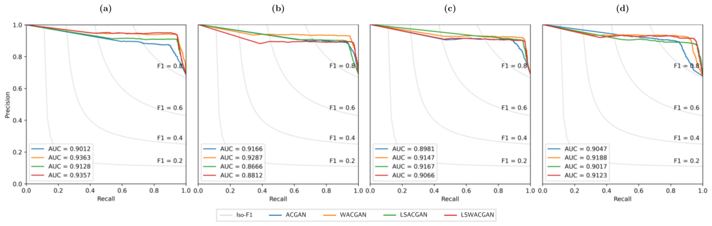
The P-R curves in Figure 8 and Figure 9 reveal the impact of ablation on the precision–recall balance across all possible thresholds in both examined scenarios. In the multi-class scenario, a striking gap in PR-AUC scores between LSWACGAN and its ablated counterparts is observed. This gap widens with increasing magnification, showing a clear trend of progressive improvement. Conversely, the binary scenario sees the ablated variants catching up at higher magnification levels. WACGAN is found to yield better precision and recall than ACGAN and LSACGAN over the full range of magnification levels, which once again echoes the other performance results presented in Table 4 and Table 5. Even with limited training data, LSWACGAN attains PR-AUC scores exceeding $0.5$ for all classes (subtypes) in the more complex multi-class scenario. This confirms that mixing all components together produces a strong, reliable model, capable of performing well on each class individually, regardless of their prevalence. Confusion matrices for LSWACGAN and ablated variants in the multi-class scenario are similarly displayed in Figure 10. Here too, there is a discernible boost in performance—particularly at the lowest magnification level—for the proposed LSWACGAN classifier, although WACGAN and LSACGAN appear to show more uniform confusion among classes as the magnification grows. Nonetheless, their overall uncertainty is still greater compared to the LSWACGAN, as tables in (b)–(d) demonstrate. At higher magnification levels, almost all the classes remain clearly distinguishable by the proposed LSWACGAN classifier, whereas a high degree of uncertainty creeps in for class (subtype) F in the case of WACGAN, and classes (subtypes) F and TA for LSACGAN. The standard ACGAN consistently records the lowest confidence among the studied variants.

To verify the findings laid out beforehand, a Tukey’s test (or Tukey’s Honestly Significant Difference, HSD) is used as a post hoc analysis to compare all pairwise means while controlling for type I error rates. Analysis of variance (ANOVA) helps the researchers identify the presence of a statistically significant effect; however, when making multiple comparisons, it is essential to carefully evaluate the family error rate because the chances of making a type I error—a.k.a, falsely rejecting the experimental hypothesis—are greater for a series of comparisons than for any single comparison. Tukey’s HSD is probably the most common and popular statistical tool utilized to determine if the relationships between three or more groups of observations are statistically significant—that is, whether the perceived differences in group mean values are unlikely to have occurred by random chance. It should be noted, though, that this method indicates association, but does not establish causality. To mitigate the risk of inflated error rates, Tukey’s method calculates and adjusts the confidence level for each individual comparison to maintain the family error rate, thereby ensuring that the overall simultaneous confidence level equals the intended nominal value.

Tables

Table 6. Adjusted p-values from Tukey’s Honestly Significant Difference test for binary ablation study.

Pair	Magnification	${\mathit{P}}_{\mathit{adj}}$
		Accuracy	Precision	Recall	Specificity	F1-Score	PR-AUC
ACGAN vs. WACGAN	$40\times$	0.0275	0.3267	0.4976	0.3598	0.0237	0.8877
	$100\times$	0.3740	0.7950	0.9763	0.8609	0.4068	0.9987
	$200\times$	0.1422	0.9982	0.4608	0.9962	0.1643	0.9960
	$400\times$	0.4088	0.3799	0.8214	0.7904	0.5108	0.9781
ACGAN vs. LSACGAN	$40\times$	0.2077	0.7996	0.5747	0.8553	0.1674	0.9980
	$100\times$	0.9981	0.9987	0.9993	1.0000	0.9985	0.7969
	$200\times$	0.4801	0.9999	0.6246	1.0000	0.4473	0.9939
	$400\times$	0.4810	0.9578	0.3830	0.7304	0.4732	1.0000
ACGAN vs. LSWACGAN	$40\times$	0.0254	0.2608	0.6218	0.2782	0.0230	0.8943
	$100\times$	0.7412	0.9998	0.8402	1.0000	0.7011	0.9298
	$200\times$	0.3007	0.9990	0.4350	0.9998	0.2843	0.9997
	$400\times$	0.1466	0.7242	0.3973	0.9701	0.2231	0.9979
WACGAN vs. LSACGAN	$40\times$	0.7986	0.9096	0.9999	0.8922	0.8263	0.9710
	$100\times$	0.5371	0.9120	0.9966	0.8727	0.5660	0.6459
	$200\times$	0.9193	0.9921	0.9985	0.9891	0.9580	1.0000
	$400\times$	0.9999	0.1319	0.9323	0.1757	1.0000	0.9572
WACGAN vs. LSWACGAN	$40\times$	1.0000	0.9999	0.9995	0.9997	1.0000	1.0000
	$100\times$	0.9650	0.8705	0.9910	0.8862	0.9851	0.8238
	$200\times$	0.9891	0.9807	1.0000	0.9838	0.9966	0.9998
	$400\times$	0.9589	0.9725	0.9401	0.9852	0.9723	0.9989
LSACGAN vs. LSWACGAN	$40\times$	0.7777	0.8483	1.0000	0.8132	0.8196	0.9738
	$100\times$	0.8843	1.0000	0.9296	1.0000	0.8482	0.9974
	$200\times$	0.9963	1.0000	0.9972	1.0000	0.9970	0.9994
	$400\times$	0.9245	0.3418	1.0000	0.3784	0.9818	0.9926

Boldface denotes statistically significant results (i.e., $p<0.05$).

and

Table 7. Adjusted p-values from Tukey’s Honestly Significant Difference test for multi-class ablation study.

Pair	Magnification	${\mathit{P}}_{\mathit{adj}}$
		Accuracy	Precision	Recall	Specificity	F1-Score	PR-AUC
ACGAN vs. WACGAN	$40\times$	0.0040	0.0010	0.0001	0.0032	0.0002	0.0408
	$100\times$	0.5945	0.5119	0.3005	0.3701	0.3156	0.9819
	$200\times$	0.0000	0.0000	0.0014	0.0000	0.0000	0.0000
	$400\times$	0.0029	0.1767	0.0242	0.0007	0.0165	0.0283
ACGAN vs. LSACGAN	$40\times$	0.0519	0.0155	0.0013	0.0320	0.0040	0.5167
	$100\times$	0.7189	0.3098	0.7089	0.6128	0.7079	0.9969
	$200\times$	0.0001	0.0084	0.1204	0.0001	0.0007	0.0001
	$400\times$	0.0318	0.3463	0.1278	0.0105	0.1578	0.1243
ACGAN vs. LSWACGAN	$40\times$	0.0016	0.0010	0.0000	0.0013	0.0001	0.0257
	$100\times$	0.1432	0.1982	0.3688	0.0883	0.2021	0.5073
	$200\times$	0.0000	0.0002	0.0017	0.0000	0.0000	0.0000
	$400\times$	0.0014	0.0272	0.0046	0.0003	0.0033	0.0131
WACGAN vs. LSACGAN	$40\times$	0.7001	0.6446	0.6778	0.7791	0.4696	0.5371
	$100\times$	0.9995	0.9947	0.9425	0.9920	0.9514	0.9996
	$200\times$	0.3377	0.0638	0.1987	0.1554	0.0252	0.4744
	$400\times$	0.7519	0.9914	0.8982	0.6464	0.7502	0.9299
WACGAN vs. LSWACGAN	$40\times$	0.9907	1.0000	0.9711	0.9889	0.9909	0.9992
	$100\times$	0.8445	0.9579	0.9999	0.8977	0.9982	0.8136
	$200\times$	0.9935	0.8671	0.9999	0.9972	1.0000	0.9960
	$400\times$	0.9949	0.8444	0.9156	0.9884	0.9260	0.9947
LSACGAN vs. LSWACGAN	$40\times$	0.4384	0.6434	0.3365	0.5062	0.2543	0.4044
	$100\times$	0.7361	0.9983	0.9733	0.6839	0.8509	0.7056
	$200\times$	0.1808	0.3228	0.2412	0.0869	0.0317	0.2932
	$400\times$	0.5282	0.6027	0.4496	0.3758	0.3074	0.7636

Boldface denotes statistically significant results (i.e., $p<0.05$).

outline the results of Tukey’s HSD test for binary and multi-class scenarios. Using a confidence level of $95\%$, the null hypothesis of no significant difference in performance means between contrasting models is rejected for all tests with an adjusted p-value smaller than $0.05$, indicated by the boldface typed values. In the binary scenario, the introduction of the Wasserstein loss with a gradient penalty yields marginally better results on a limited subset of performance metrics, observable only at the lowest magnification level, compared to the standard ACGAN. Alternatively, all three enhanced variants demonstrate superior performance (i.e., $p<0.05$) to that of the standard ACGAN over all selected evaluation metrics in a multi-class scenario. Nevertheless, the mean differences among the three of them are, for the most part, statistically insignificant, indicating that there is insufficient evidence to support the claim that any one of them performs differently than the others. This suggests that the variants’ performance is inconsistent across different tests and data subsets, leading to a high standard deviation that masks the mean difference. In the context of an ablation study, this might be grounds to conclude that one or the other proposed enhancement is nonessential, as their removal does not produce a statistically measurable change in performance. Having acknowledged that, we should remember that the absence of evidence is not evidence of absence and that results that do not reach statistical significance may still hold clinical relevance, particularly when considering effect sizes, confidence intervals, and patient outcomes. Moreover, p-values and tests of statistical significance do not reveal anything about the effect size or its practical importance. In a large sample, a difference that is statistically significant might be trivial; in a small sample, substantively important differences might not reach statistical significance [61]. Therefore, it would be wrong to hastily assume that all three enhanced variants are truly equivalent. A non-significant result simply means that no evidence of a difference was found at this time and that further investigation or follow-up studies are warranted to confirm that the previously described, noticeable trend of improvement with the full model is real.

6. Conclusions

This work focuses on developing a novel framework for classifying breast cancer histopathological images that can yield strong success rates while simultaneously grappling with important challenges, like class imbalance and complex class structures. The proposed system uses an enhanced ACGAN as a “one-stop-shop” solution, leveraging its auxiliary branch for classification purposes. By combining and jointly optimizing the data generation and classification modules, the proposed model can both produce new samples to improve the generalization and accurately categorize samples into their respective classes. Incorporating label smoothing and gradient-penalty Wasserstein loss enables the model to learn more distinguishable features across different classes. The LSWACGAN model holds its ground and performs comparably to two state-of-the-art supervised baseline classifiers in the binary classification scenario. Its true strength, however, shines in the multi-class scenario, where it consistently demonstrates superior performance over its competitors at all magnification levels, even with a limited training repertoire. Better PR-AUC scores across most tumor classes, reduced class confusion, and higher classifier confidence are a further testament to the model’s effectiveness for multi-class breast tumor subtype classification. While these results are encouraging, the current study has several limitations that must be acknowledged. First, it is noteworthy that the results may have been afflicted, to some extent, by restricting image analysis to a resolution of $224\times 224$ pixels to match the input requirements of the baseline models. Moreover, the LSWACGAN was trained and evaluated primarily on a single dataset, potentially limiting its generalizability to other histopathological data. Although BreakHis is widely recognized as a benchmark dataset for breast cancer histopathology image analysis, it may not reflect the full diversity of real-world clinical data. Consequently, the model’s performance should be validated with a broader set of datasets from different geographic regions and populations to ensure consistency across demographics and make it more practical and applicable to various scenarios.

Looking ahead, future work will attempt to address the identified limitations and will also include fine-tuning the generator and discriminator architectures, applying more advanced training techniques—such as adaptive discriminator augmentation or progressive growing—and experimenting with alternative generative frameworks to further boost generalization performance.

References

1. Ferlay, J.; Ervik, M.; Lam, F.; Laversanne, M.; Colombet, M.; Mery, L.; Piñeros, M.; Znaor, A.; Soerjomataram, I.; Bray, F. Global Cancer Observatory: Cancer Today. 2024. Available online: https://gco.iarc.who.int/today (accessed on 20 April 2026).
2. European Commision. ECIS: European Cancer Information System. Available online: https://ecis.jrc.ec.europa.eu/ (accessed on 20 April 2025).
3. Yassin, N.I.; Omran, S.; Houby, E.M.; Allam, H. Machine learning techniques for breast cancer computer aided diagnosis using different image modalities: A systematic review. Comput. Methods Programs Biomed. 2018, 156, 25–45. [Google Scholar] [CrossRef] [Scilit] [PubMed]
4. Bhatt, C.; Kumar, I.; Vijayakumar, V.; Singh, K.U.; Kumar, A. The state of the art of deep learning models in medical science and their challenges. Multimed. Syst. 2020, 27, 599–613. [Google Scholar] [CrossRef] [Scilit]
5. Abhisheka, B.; Biswas, S.K.; Purkayastha, B.; Das, D.; Escargueil, A. Recent trend in medical imaging modalities and their applications in disease diagnosis: A review. Multim. Tools Appl. 2023, 83, 43035–43070. [Google Scholar] [CrossRef] [Scilit]
6. Dhar, T.; Dey, N.; Borra, S.; Sherratt, R.S. Challenges of deep learning in medical image analysis—Improving explainability and trust. IEEE Trans. Technol. Soc. 2023, 4, 68–75. [Google Scholar] [CrossRef] [Scilit]
7. Yang, L.; Zhang, Z.; Song, Y.; Hong, S.; Xu, R.; Zhao, Y.; Zhang, W.; Cui, B.; Yang, M.-H. Diffusion models: A comprehensive survey of methods and applications. ACM Comput. Surv. 2024, 56, 105. [Google Scholar] [CrossRef] [Scilit]
8. Kingma, D.; Welling, M. Auto-encoding variational Bayes. In Proceedings of the 2nd International Conference on Learning Representations (ICLR), Banff, AB, Canada, 14–16 April 2014; pp. 1–14. [Google Scholar]
9. Goodfellow, I.; Pouget-Abadie, J.; Mirza, M.; Xu, B.; Warde-Farley, D.; Ozair, S.; Courville, A.; Bengio, Y. Generative adversarial nets. Adv. Neural Inf. Process. Syst. 2014, 2, 2672–2680. [Google Scholar] [CrossRef] [Scilit]
10. Kantorovich, L.V.; Rubinstein, G.S. On a space of totally additive functions. Vestn. Leningr. Univ. 1958, 13, 52–59. [Google Scholar]
11. Clement David-Olawade, A.; Olawade, D.B.; Vanderbloemen, L.; Rotifa, O.B.; Fidelis, S.C.; Egbon, E.; Akpan, A.O.; Adeleke, S.; Ghose, A.; Boussios, S. AI-driven advances in low-dose imaging and enhancement—A review. Diagnostics 2025, 15, 689. [Google Scholar] [CrossRef] [Scilit] [PubMed]
12. Yang, G.; Yu, S.; Dong, H.; Slabaugh, G.; Dragotti, P.L.; Ye, X.; Liu, F.; Arridge, S.; Keegan, J.; Guo, Y.; et al. DAGAN: Deep de-aliasing generative adversarial networks for fast compressed sensing MRI reconstruction. IEEE Trans. Med. Imaging 2018, 37, 1310–1321. [Google Scholar] [CrossRef] [Scilit] [PubMed]
13. Kim, K.H.; Do, W.-J.; Park, S.-H. Improving resolution of MR images with an adversarial network incorporating images with different contrast. Med. Phys. 2018, 45, 3120–3131. [Google Scholar] [CrossRef] [Scilit] [PubMed]
14. Hou, B.; Du, H. MCA-GAN: A lightweight multi-scale context-aware generative adversarial network for MRI reconstruction. Magn. Reson. Imaging 2025, 124, 110465. [Google Scholar] [CrossRef] [Scilit] [PubMed]
15. Nie, D.; Trullo, R.; Lian, J.; Wang, L.; Petitjean, C.; Ruan, S.; Wang, X.; Shen, D. Medical image synthesis with deep convolutional adversarial networks. IEEE Trans. Biomed. Eng. 2018, 65, 2720–2730. [Google Scholar] [CrossRef] [Scilit] [PubMed]
16. Yang, Q.; Yan, P.; Zhang, Y.; Yu, H.; Shi, Y.; Mou, X.; Kalra, M.K.; Zhang, Y.; Sun, L.; Wang, G. Low-dose CT image denoising using a generative adversarial network with Wasserstein distance and perceptual loss. IEEE Trans. Med. Imaging 2018, 37, 1348–1357. [Google Scholar] [CrossRef] [Scilit] [PubMed]
17. Di Feola, F.; Tronchin, L.; Guarrasi, V.; Soda, P. Multi-scale texture loss for CT denoising with GANs. arXiv 2024, arXiv:2403.16640. [Google Scholar]
18. Wang, J.; Zhao, Y.; Noble, J.H.; Dawant, B.M. Conditional generative adversarial networks for metal artifact reduction in CT images of the ear. In Proceedings of the 21st International Conference on Medical Image Computing and Computer-Assisted Intervention (MICCAI), Granada, Spain, 16–20 September 2018; pp. 3–11. [Google Scholar] [CrossRef] [Scilit] [PubMed]
19. Pande, P.; Misba, M.; Gupta, D.; Rani, V.K.; Ahmed, H.S.; Balakumar, A. Adversarial artifact removal: A GAN-based framework for enhanced image quality and reliability. In Proceedings of the 5th International Conference on Advances in Electrical, Computing, Communication and Sustainable Technologies (ICAECT), Bhilai, India, 9–10 January 2025; pp. 1–6. [Google Scholar] [CrossRef] [Scilit]
20. Gu, Y.; Zeng, Z.; Chen, H.; Wei, J.; Zhang, Y.; Chen, B.; Li, Y.; Qin, Y.; Xie, Q.; Jiang, Z.; et al. MedSRGAN: Medical images super-resolution using generative adversarial networks. Multimed. Tools Appl. 2020, 79, 21815–21840. [Google Scholar] [CrossRef] [Scilit]
21. Shahidi, F. Breast cancer histopathology image super-resolution using wide-attention GAN with improved Wasserstein gradient penalty and perceptual loss. IEEE Access 2021, 9, 32795–32809. [Google Scholar] [CrossRef] [Scilit]
22. Jha, A.; Iima, H. CT to MRI image translation using CycleGAN: A deep learning approach for cross-modality medical imaging. In Proceedings of the 16th International Conference on Agents and Artificial Intelligence (ICAART), Rome, Italy, 23–25 February 2024; pp. 951–957. [Google Scholar] [CrossRef] [Scilit]
23. Sun, H.; Jiang, Y.; Yuan, J.; Wang, H.; Liang, D.; Fan, W.; Hu, Z.; Zhang, N. High-quality PET image synthesis from ultra-low-dose PET/MRI using bi-task deep learning. Quant. Imaging Med. Surg. 2022, 12, 5326–5342. [Google Scholar] [CrossRef] [Scilit] [PubMed]
24. Salehjahromi, M.; Karpinets, T.V.; Sujit, S.J.; Qayati, M.; Chen, P.; Aminu, M.; Saad, M.B.; Bandyopadhyay, R.; Hong, L.; Sheshadri, A.; et al. Synthetic PET from CT improves diagnosis and prognosis for lung cancer: Proof of concept. Cell Rep. Med. 2024, 5, 101463. [Google Scholar] [CrossRef] [Scilit] [PubMed]
25. Armanious, K.; Jiang, C.; Fischer, M.; Kustner, T.; Hepp, T.; Nikolaou, K.; Gatidis, S.; Yang, B. MedGAN: Medical image translation using GANs. Comput. Med. Imaging Graph. 2020, 79, 101684. [Google Scholar] [CrossRef] [Scilit] [PubMed]
26. Xu, Z.; Wang, X.; Shin, H.-C.; Yang, D.; Roth, H.; Milletari, F.; Zhang, L.; Xu, D. Correlation via synthesis: End-to-end image generation and radiogenomic learning based on generative adversarial network. Proc. Mach. Learn. Res. 2020, 121, 857–866. [Google Scholar] [CrossRef] [Scilit]
27. Cohen, J.P.; Luck, M.; Honari, S. Distribution matching losses can hallucinate features in medic image translation. In Proceedings of the International Conference on Medical Image Computing and Computer-Assisted Intervention (MICCAI), Granada, Spain, 16–20 September 2018; pp. 529–536. [Google Scholar] [CrossRef] [Scilit]
28. Wu, E.; Wu, K.; Cox, D.; Lotter, W. Conditional infilling GANs for data augmentation in mammogram classification. In Image Analysis for Moving Organ, Breast, and Thoracic Images; Springer: Berlin/Heidelberg, Germany, 2018; pp. 98–106. [Google Scholar]
29. Jendele, L.; Skopek, O.; Becker, A.S.; Konukoglu, E. Adversarial augmentation for enhancing classification of mammography images. arXiv 2019, arXiv:1902.07762. [Google Scholar]
30. Jiménez-Gaona, Y.; Carrión-Figueroa, D.; Lakshminarayanan, V.; Rodríguez-Álvarez, M.J. GAN-based data augmentation to improve breast ultrasound and mammography mass classification. Biomed. Signal Process. Control 2024, 94, 106255. [Google Scholar] [CrossRef] [Scilit]
31. Schlegl, T.; Seebock, P.; Waldstein, S.M.; Langs, G.; Schmidt-Erfurth, U. f-AnoGAN: Fast unsupervised anomaly detection with generative adversarial networks. Med. Image Anal. 2019, 54, 30–44. [Google Scholar] [CrossRef] [Scilit] [PubMed]
32. Kuang, Y.; Lan, T.; Peng, X.; Selasi, G.E.; Liu, Q.; Zhang, J. Unsupervised multi-discriminator generative adversarial network for lung nodule malignancy classification. IEEE Access 2020, 8, 77725–77734. [Google Scholar] [CrossRef] [Scilit]
33. Nakao, T.; Hanaoka, S.; Nomura, Y.; Murata, M.; Takenaga, T.; Miki, S.; Watadani, T.; Yoshikawa, T.; Hayashi, N.; Abe, O. Unsupervised deep anomaly detection in chest radiographs. J. Digit. Imaging 2021, 34, 418–427. [Google Scholar] [CrossRef] [Scilit] [PubMed]
34. Lee, S.; Jeong, B.; Kim, M.; Jang, R.; Paik, W.; Kang, J.; Chung, W.J.; Hong, G.-S.; Kim, N. Emergency triage of brain computed tomography via anomaly detection with a deep generative model. Nat. Commun. 2022, 13, 4251. [Google Scholar] [CrossRef] [Scilit] [PubMed]
35. Li, H.; Xie, J.; Ke, J.; Yuan, Y.; Pan, X.; Xin, H.; Shen, H. GAN-DIRNet: A novel deformable image registration approach for multimodal histological images. Comput. Mater. Contin. 2024, 80, 487–506. [Google Scholar] [CrossRef] [Scilit]
36. Cirillo, M.D.; Abramian, D.; Eklund, A. Vox2Vox:3D-GAN for brain tumour segmentation. arXiv 2020, arXiv:2003.13653. [Google Scholar]
37. Shi, Z.; Hu, Q.; Yue, Y.; Wang, Z.; Alothmani, O.M.S.; Li, H. Automatic nodule segmentation method for CT images using aggregation-UNet generative adversarial aetworks. Sens. Imaging 2020, 21, 39. [Google Scholar] [CrossRef] [Scilit]
38. Xia, W.; Zhang, Y.; Yang, Y.; Xue, J.H.; Zhou, B.; Yang, M.H. GAN inversion: A survey. IEEE Trans. Pattern Anal. Mach. Intell. 2022, 45, 3121–3138. [Google Scholar] [CrossRef] [PubMed]
39. Ren, Z.; Yu, S.X.; Whitney, D. Controllable medical image generation via GAN. J. Percept. Imaging 2022, 5, 000502. [Google Scholar] [CrossRef] [Scilit] [PubMed]
40. Golhar, M.; Bobrow, T.; Ngamruengphong, S.; Durr, N. GAN inversion for data augmentation to improve colonoscopy lesion classification. IEEE J. Biomed. Health Inform. 2025, 29, 3864–3873. [Google Scholar] [CrossRef] [Scilit] [PubMed]
41. Mirsky, Y.; Mahler, T.; Shelef, I.; Elovici, Y. CT-GAN: Malicious tampering of 3d medical imagery using deep learning. In Proceedings of the 28th USENIX Security Symposium, Santa Clara, CA, USA, 14–16 August 2019; pp. 461–478. [Google Scholar] [CrossRef] [Scilit]
42. Schwarz, C.G.; Kremers, W.K.; Therneau, T.M.; Sharp, R.R.; Gunter, J.L.; Vemuri, P.; Arani, A.; Spychalla, A.J.; Kantarci, K.; Knopman, D.S.; et al. Identification of anonymous mri research participants with face-recognition software. N. Engl. J. Med. 2019, 381, 1684–1686. [Google Scholar] [CrossRef] [Scilit] [PubMed]
43. Van der Goten, L.A.; Hepp, T.; Akata, Z.; Smith, K. Conditional de-identification of 3D magnetic resonance images. arXiv 2021, arXiv:2110.09927. [Google Scholar]
44. Marchesi, R.; Micheletti, N.; I-Hsien Kuo, N.; Barbieri, S.; Jurman, G.; Osmani, V. Generative AI mitigates representation bias and improves model fairness through synthetic health data. PLoS Comput. Biol. 2025, 21, e1013080. [Google Scholar] [CrossRef] [Scilit] [PubMed]
45. Yoon, J.; Jordon, J.; Schaar, M. GANITE: Estimation of individualized treatment effects using generative adversarial nets. In Proceedings of the 6th International Conference on Learning Represenations (ICLR), Vancouver, BC, Canada, 30 April–3 May 2018; pp. 2196–2218. [Google Scholar]
46. Wang, J.; Wan, H.; Chen, X. GANCQR: Estimating prediction intervals for individual treatment effects with GANs. In Proceedings of the 2024 Winter Simulation Conference (WSC), Orlando, FL, USA, 15–18 December 2024; pp. 2571–2582. [Google Scholar] [CrossRef] [Scilit]
47. Kuang, K.; Li, Y.; Li, B.; Cui, P.; Yang, H.; Tao, J.; Wu, F. Continuous treatment effect estimation via generative adversarial de-confounding. Data Min. Knowl. Discov. 2021, 35, 2467–2497. [Google Scholar] [CrossRef] [Scilit]
48. Wang, R.; Bashyam, V.; Yang, Z.; Yu, F.; Tassopoulou, V.; Chintapalli, S.S.; Skampardoni, I.; Sreepada, L.P.; Sahoo, D.; Nikita, K.; et al. Applications of generative adversarial networks in neuroimaging and clinical neuroscience. NeuroImage 2024, 269, 119898. [Google Scholar] [CrossRef] [Scilit] [PubMed]
49. Mescheder, L.; Nowozin, S.; Geiger, A. The numerics of GANs. In Proceedings of the 31st International Conference on Neural Information Processing Systems (NIPS), Long Beach, CA, USA, 4–6 December 2017; pp. 1823–1833. [Google Scholar]
50. Lin, J. Divergence measures based on the Shannon entropy. IEEE Trans. Inf. Theory 1991, 37, 145–151. [Google Scholar] [CrossRef] [Scilit]
51. Villani, C. The Wasserstein distances. In Optimal Transport: Old and New; Springer: Berlin/Heidelberg, Germany, 2008; pp. 93–111. [Google Scholar]
52. Kullback, S.; Leibler, R.A. On information and sufficiency. Ann. Math. Stat. 1951, 22, 79–86. [Google Scholar] [CrossRef] [Scilit]
53. Gulrajani, I.; Ahmed, F.; Arjovsky, M.; Dumoulin, V.; Courville, A.C. Improved training of Wasserstein GANs. In Proceedings of the 31st International Conference on Neural Information Processing Systems (NIPS), Long Beach, CA, USA, 4–6 December 2017; pp. 5769–5779. [Google Scholar]
54. Odena, A.; Olah, C.; Shlens, J. Conditional image synthesis with auxiliary classifier GANs. In Proceedings of the 34th International Conference on Machine Learning (ICML), Sydney, Australia, 6–11 August 2017; pp. 2642–2651. [Google Scholar]
55. Spanhol, F.A.; Oliveira, L.S.; Petitjean, C.; Heutte, L. A dataset for breast cancer histopathological image classification. IEEE Trans. Biomed. Eng. 2016, 63, 1455–1462. [Google Scholar] [CrossRef] [Scilit] [PubMed]
56. Pizer, S.M.; Amburn, E.P.; Austin, J.D.; Cromartie, R.; Geselowitz, A.; Greer, T.; Romeny, B.M.; Zimmerman, J.B.; Zuiderveld, K. Adaptive histogram equalization and its variations. Comput. Vis. Graph. Image Process. 1987, 39, 355–368. [Google Scholar] [CrossRef] [Scilit]
57. Maas, A.L.; Hannun, A.Y.; Ng, A.Y. Rectifier Nonlinearities Improve Neural Network Acoustic Models. In Proceedings of the 30th International Conference on Machine Learning (ICML), Atlanta, GA, USA, 16–21 June 2013; pp. 1–6. [Google Scholar]
58. Saito, T.; Rehmsmeier, M. The Precision-Recall Plot Is More Informative than the ROC Plot When Evaluating Binary Classifiers on Imbalanced Dataset. PLoS ONE 2015, 4, e0118432. [Google Scholar] [CrossRef] [Scilit] [PubMed]
59. Huang, G.; Liu, Z.; van der Maaten, L.; Weinberger, K.Q. Densely Connected Convolutional Networks. In Proceedings of the 2017 IEEE Conference on Computer Vision and Pattern Recognition (CVPR), Honolulu, HI, USA, 21–26 July 2017; pp. 4700–4708. [Google Scholar] [CrossRef] [Scilit]
60. Tan, M.; Le, Q.V. EfficientNet: Rethinking Model Scaling for Convolutional Neural Networks. In Proceedings of the 36th International Conference on Machine Learning (ICML), Long Beach, CA, USA, 9–15 June 2019; pp. 6105–6114. [Google Scholar] [CrossRef] [Scilit]
61. Yaddanapudi, L.N. The American Statistical Association Statement on P-Values Explained. J. Anaesthesiol. Clin. Pharmacol. 2016, 32, 421–423. [Google Scholar] [CrossRef] [Scilit] [PubMed]
62. Alzoubi, H.; Madain, R.; Amin, M.; Madae’en, S.; Aljehani, A.M.; Serhan, H.A.; Alhatamleh, S.; Alomani, A. Enhancing Breast Cancer Diagnosis with ResNet50 and Salp Swarm-Based Feature Reduction on BreakHis Dataset. Biomed. Signal Process. Control 2026, 114, 109319. [Google Scholar] [CrossRef] [Scilit]
63. Aneesha, J.; Zoheir, E. Breast Cancer Detection Using BCDNet Convolutional Neural Network. Array 2026, 29, 100711. [Google Scholar] [CrossRef] [Scilit]
64. Zeng, L.; Qin, M.; Hu, J.; Cai, S.; Wang, S. A Center-Border Dual-Branch Network With Dynamic Weighted Fusion for Breast Cancer Histopathology Image Classification. Int. J. Imaging Syst. Technol. 2026, 36, e70341. [Google Scholar] [CrossRef] [Scilit]
65. Bohra, M.; Singh, K.U.; Kumar, I.; Shah, M.A. Wavelet-CNN Feature Fusion Architecture for Robust Breast Cancer Classification in Histopathological Imaging. Int. J. Comput. Intell. Syst. 2026, 19, 136. [Google Scholar] [CrossRef] [Scilit]
66. Desai, A.; Mahto, R. Multi-Class Classification of Breast Cancer Subtypes Using ResNet Architectures on Histopathological Images. J. Imaging 2025, 11, 284. [Google Scholar] [CrossRef] [Scilit] [PubMed]
67. Wakili, M.A.; Shehu, H.A.; Abdollahi, M.; Ya’u, B.I.; Sharif, H.; Kusetogullari, H. DenseNet-FPA: Integrating DenseNet and Flower Pollination Algorithm for Breast Cancer Histopathology Image Classification. IEEE Access 2025, 13, 145828–145848. [Google Scholar] [CrossRef] [Scilit]
68. Alshehri, H. BreNet: Attention-Enhanced Multi-Scale CNN Framework for Breast Cancer Classification in Histopathological Images. IEEE Access 2025, 13, 143377–143391. [Google Scholar] [CrossRef] [Scilit]
69. Arshad, W.; Masood, T.; Shahzad, H.M.; Ahmed, H.; Ahmed, S.H.; Tayyab Khushi, H.M. HistoDX: Revolutionizing Breast Cancer Diagnosis Through Advanced Imaging Techniques. IEEE Access 2025, 13, 94416–94436. [Google Scholar] [CrossRef] [Scilit]
70. Zhao, M.; Hou, C.; Cao, L.; Zhang, J. Breast Cancer Histopathological Image Classification Based on High-Order Modeling and Multi-Branch Receptive Fields. Appl. Sci. 2025, 15, 6085. [Google Scholar] [CrossRef] [Scilit]
71. Jia, Y.; Hao, S.; Liu, J.; Liu, C.; Ji, Z.; Ganchev, I. DenLsNet-C: A Novel Model for Breast Cancer Classification in Pathology Images Based on DenseNet and LSTM. J. Supercomput. 2025, 81, 934. [Google Scholar] [CrossRef] [Scilit]
72. Chikkala, R.B.; Anuradha, C.; Chandra Murty, P.; Rajeswari, S.; Rajeswaran, N.; Murugappan, M.; Chowdhury, M. Enhancing Breast Cancer Diagnosis With Bidirectional Recurrent Neural Networks: A Novel Approach for Histopathological Image Multi-Classification. IEEE Access 2025, 13, 41682–41707. [Google Scholar] [CrossRef] [Scilit]
Figure 1. Standard GAN (left side) and ACGAN (right side) flowchart. Standard GAN blindly generates data from random noise, whereas ACGAN uses class labels to condition the generation process. While a standard GAN’s discriminator only evaluates if an image is real or fake, the ACGAN discriminator includes an additional classification layer that predicts the specific category of both real and generated images.
Symmetry 18 01235 g001
Figure 2. Sample images from BreakHis dataset.
Symmetry 18 01235 g002
Figure 3. Enhanced ACGAN multi-tiered architecture with generator and discriminator.
Symmetry 18 01235 g003
Figure 4. Training loss of the LSWACGAN generator and discriminator for a multi-class scenario at 40 × and 400 × magnification levels.
Symmetry 18 01235 g004
Figure 5. P-R curves for binary model comparisons. Curves at 40 × , 100 × , 200 × , and 400 × magnification levels are displayed progressively in columns (ad).
Symmetry 18 01235 g005
Figure 6. P-R curves for multi-class model comparisons: DenseNet-121, EfficientNet-B0, and LSWACGAN are shown in the top, middle and bottom rows, respectively. Curves at 40 × , 100 × , 200 × , and 400 × magnification levels are displayed progressively in columns (ad).
Symmetry 18 01235 g006
Figure 7. Confusion matrices for multi-class model comparisons at 40 × , 100 × , 200 × , and 400 × magnification levels, displayed progressively in columns (ad). The successive rows from top to bottom showcase tables for DenseNet121, EfficientNetB0, and LSWACGAN, respectively.
Symmetry 18 01235 g007
Figure 8. P-R curves for binary ablation study. Curves at 40 × , 100 × , 200 × , and 400 × magnification levels are displayed progressively in columns (ad).
Symmetry 18 01235 g008
Figure 9. P-R curves for multi-class ablation study: ACGAN, WACGAN, LSACGAN, and LSWACGAN are shown in the top, upper-middle, lower-middle and bottom rows, respectively. Curves at 40 × , 100 × , 200 × , and 400 × magnification levels are displayed progressively in columns (ad).
Symmetry 18 01235 g009
Figure 10. Confusion matrices for multi-class ablation study at 40 × , 100 × , 200 × , and 400 × magnification levels, displayed progressively in columns (ad). The successive rows from top to bottom showcase tables for ACGAN, WACGAN, LSACGAN, and LSWACGAN, respectively.
Symmetry 18 01235 g010