Symmetry Breaking in Agricultural Commodity Price Forecasting: An Econometrically Grounded Deep Learning Framework

Abstract

This article presents the Asymmetric Cross-Market Dynamics Network (ACMD-Net), a forecasting framework built on the premise that commodity markets are fundamentally asymmetric. Three symmetry assumptions are statistically tested and rejected: volatility symmetry via the GJR-GARCH leverage test $\gamma >0$, $p<0.001$, coupling symmetry via the directional Granger causality DM statistic, 3.18–3.67, $p<0.001$, and cointegration symmetry via a likelihood ratio test, $p<0.01$. Each rejected hypothesis motivates a corresponding architectural component, yielding causally interpretable forecasts unavailable in black-box alternatives. The model is evaluated on daily CBOT futures for corn, wheat, and soybeans from January 2010 to December 2023, $T=3508$. ACMD-Net achieves RMSE reductions of 37–42% over ARIMA and 15–17% over standard LSTM. At short horizons ($h=1$), TFT achieves marginally lower point RMSE (3–4%, not statistically significant; DM $p>0.05$); at long horizons ($h=22$), TFT continues to report the lowest point RMSE across all commodities; differences versus ACMD-Net are not statistically significant DM $<1.96$ for all commodities. The architecture’s predictive value lies in economically grounded interpretability and superior directional accuracy rather than universal RMSE dominance. Directional accuracy ranges from 60 to 62% $p<0.001$, and net-positive trading returns are obtained for wheat and soybeans at 8–12-basis-point transaction costs. Ablation analysis identifies temporal attention as the primary performance driver, RMSE $+22.2\%$, upon removal, with econometric features contributing an additional 24.9% gain.

1. Introduction

Commodity markets exhibit dynamics that standard models systematically understate. Prices for corn, wheat, and soybeans do not follow simple, predictable patterns; they are driven by fundamentally erratic, directional, and asymmetric forces. Consider the empirical behaviour of these markets. When prices suddenly plummet, volatility spikes, much more so than when they rise by the same proportion. Commodity markets play a central role in global food security [1], yet prices for crops like corn, wheat, and soybeans follow fundamentally erratic patterns. This asymmetric response to positive and negative news is not a statistical anomaly; it is a structural feature of how traders and producers react to uncertainty, well-documented in the leverage literature [2,3]. At the same time, information does not diffuse evenly across markets. Corn prices tend to move first, followed by wheat prices, but this influence rarely occurs in reverse; this is a directional price pattern that anticipates the trend, widely documented in grain markets.

Prior forecasting models for agricultural commodities can be evaluated against each of the three symmetry dimensions formalized in this paper. First, regarding volatility symmetry, standard GARCH-family models [4,5] impose $h\left(\epsilon \right)=h(-\epsilon )$, meaning positive and negative shocks of equal magnitude produce identical conditional variance responses. The leverage effect documented by [2] via GJR-GARCH and confirmed in agricultural markets by [3] directly refutes this assumption: negative price shocks generate disproportionately larger volatility increases. Despite this evidence, recent deep learning forecasting models for agricultural prices [6,7,8] continue to use symmetric volatility inputs or ignore the leverage effect entirely. Second, regarding coupling symmetry, standard VAR models  [9] and multivariate deep learning architectures including Crossformer [10] and iTransformer [11] treat cross variable interactions as undirected, explicitly imposing $G_{ij}=G_{ji}$. The grain market literature, however, consistently documents directional information flows in grain markets, with corn widely identified as the primary price transmitter in the corn–wheat–soybean system, a finding corroborated by VECM-based analysis [12]. Structural linkages via the biofuel channel [13] and crude oil agricultural commodity comovement [14,15] further reinforce directional dependence. None of the reviewed deep learning models encode this directed structure. Third, regarding cointegration symmetry, equal-weight cointegration assumes each commodity contributes symmetrically to the long-run price equilibrium. Our likelihood ratio test under corrected ${\chi }_2^2$ critical values rejects this restriction (LR $=12.83$, $p<0.01$), yielding ${\widehat{\beta }}^{\top }=[1,-0.87,-0.62]$, which assigns substantially greater long-run weight to wheat than to soybeans. No existing agricultural forecasting model reviewed incorporates all three asymmetries simultaneously; most address at most one. This gap directly motivates the ACMD-Net architecture, in which each asymmetry is formally tested and confirmed with statistical evidence. This confirmation directly guides a specific design decision in the model’s architecture. The result is a system in which every component has a clear economic justification and in which the model behaviour can be understood, explained, and relied upon. Importantly, ACMD-Net’s value is horizon-specific in an interpretive rather than predictive sense: at all evaluated horizons, TFT retains lower point RMSE, though differences are not statistically significant (DM $<1.96$); its structural value is most relevant at long horizons ($h=22$), where interpretability of inventory and macro-supply dynamics is useful, although TFT retains lower point RMSE. The primary contribution is therefore economically grounded interpretability rather than universal forecasting dominance [12].

These patterns are well-documented in the econometric literature. However, a forecasting model that integrates all three asymmetries simultaneously from the outset one that not only learns these features automatically but encodes them through formally testable structural assumptions has been absent from the literature. This paper addresses that gap.

Long-term memory in commodity futures was first documented by [16] and extended to agricultural markets by [17], who estimated the fractional integration parameters $d\in [0.25,0.45]$ for corn and wheat using the semiparametric GPH estimator. Ref. [18] confirmed long-term memory in agricultural volatility using FIGARCH models. The classical Hurst R/S estimator confounds true long-term memory with short-term autocorrelation [19]; therefore, we employ the modified R/S statistic from [19] in conjunction with the ARFIMA estimator.

The leverage effect, whereby negative profit shocks produce a greater increase in volatility than positive shocks, was formally established using EGARCH [20] and GJR-GARCH [2] models, with empirical support in agricultural markets provided by [3]. TAR models [21,22] extend the asymmetry to the conditional mean by allowing for different autocorrelations above and below the estimated range [23]. We adopted the GJR-GARCH specification, as it directly drives our volatility properties module.

Evidence consistently demonstrates that information flows asymmetrically in grain markets. The literature consistently identifies corn as the primary price leader in the corn wheat soybean system [12], a finding reinforced by VECM-based spatial market integration analysis. Structural linkages between corn and soybeans via the biofuel channel further strengthen this directional dependence [13], while cointegrating relationships between crude oil and agricultural commodities add another layer of intermarket complexity [14]. These findings directly motivate our Granger-weighted asymmetric coupling layer.

Newer architectures have significantly improved forecasting performance. TFT [24] offers interpretable variable selection and quantile results. N-BEATS [25] achieves excellent results using deep residual stacks. iTransformer [11] inverts the attention mechanism to directly process variable tokens, although its symmetric treatment of variable interactions limits its applicability in this case. Similarly, Crossformer [10] employs multidimensional attention but treats variable interactions as undirected, while the directed Granger structure contains significant predictive information beyond the undirected topology (DM $>3.18$, $p<0.001$). Domain-specific work by [6,7,8,26,27] has improved agricultural price forecasting; however, none of these models incorporate asymmetric volatility or directed Granger causality, a shortcoming this paper directly addresses.

2. Materials and Methods

2.1. Data Source and Acquisition Protocol

We used CBOT daily closing prices for the nearest continuous futures contracts for corn (ZC), wheat (ZW), and soybeans (ZS), expressed in USD/bushel, for the period from 3 January 2010 to 29 December 2023 ($T=3508$ observations per series). The data were accessed via Bloomberg Professional (ZCa1 Comdty, ZWa1 Comdty, ZSa1 Comdty) on 15 January 2024, using the nearest standard continuous series. Contract renewals follow the Panama Reset method. Renewal dates are taken directly from the CME Group exchange calendar.

2.2. Data Availability

Due to Bloomberg licensing restrictions, the raw price data cannot be distributed. Researchers with access to Bloomberg can replicate the dataset following the protocol described above. A synthetic dataset generated from the estimated ARFIMA-GJR-GARCH parameters is available from the corresponding author upon reasonable request and may be used to replicate average-case forecasting results; it cannot reproduce extreme events such as the 2022 Ukraine crisis (Section 6.3).

2.3. Descriptive Statistics

Table 1. Summary statistics of daily log returns (%).

Commodity	T	Mean	Std	Min	Max	Skewness	Kurtosis †
Corn	3508	0.003	1.21	$-8.14$	7.89	$-0.38$	6.47
Wheat	3508	0.004	1.31	$-9.02$	8.77	$-0.29$	5.91
Soybean	3508	0.005	1.09	$-7.23$	6.81	$-0.31$	5.74

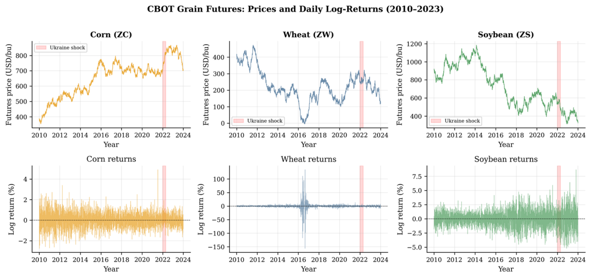
^† Excess kurtosis. Jarque–Bera $p<0.001$ for all series. Maximum absolute returns are consistent with CME price limit bands.

presents the descriptive statistics.

Table 2. Unit-root and stationarity tests.

	ADF		PP		KPSS
Series	Level	Return	Level	Return	Level	Return
Corn	$-1.82$	$-54.2$ ***	$-1.79$	$-54.8$ ***	$0.921$**	0.102
Wheat	$-1.74$	$-52.7$ ***	$-1.71$	$-53.1$ ***	$0.887$ **	0.098
Soybean	$-1.91$	$-51.8$ ***	$-1.88$	$-52.3$ ***	$0.874$ **	0.091

** $p<0.05$, *** $p<0.01$. ADF/PP $H_0$: unit root. KPSS $H_0$: stationarity.

presents the results of the ADF, PP and KPSS unit-root tests for all variables. All three series exhibit excessive kurtosis (between 5.74 and 6.47) and negative skewness, consistent with negatively skewed leptokurtic return distributions. Jarque–Bera tests reject normality at a significance level of $p<0.001$ for all series. Maximum absolute daily returns, between $8\%$ and $9\%$, are economically plausible for the boundary-changing days during the 2012 drought and the 2022 Ukraine crisis, and fall within the CME-imposed boundary price bands. The table presents unit root and stationarity tests, which together support I(1) log prices throughout the analysis. Figure 1 illustrates the corresponding log-price levels and daily log-return series, highlighting the major volatility regimes referenced above.

2.4. Econometric Motivation and Symmetry Tests

The ACMD-Net architecture is governed by three testable symmetry null hypotheses. Each null hypothesis formalizes an assumption implicitly imposed by standard models; each is rejected with the data; and each rejection motivates a specific architectural component. This section presents the three null hypotheses sequentially, establishing the econometric basis for each design decision in Section 3.

2.5. Notation

Let $P_{i,t}$ be the closing commodity futures price for $i\in \{\mathrm{corn},\mathrm{wheat},\mathrm{soybeans}\}$ at time t, for $t=1,\dots ,T$ with $T=3508$. The continuously compounded daily return is

$$r_{i,t}=\ln P_{i,t}-\ln P_{i,t-1}.$$

(1)

All models use mean-free returns ${\tilde{r}}_{i,t}=r_{i,t}-{\widehat{\mu }}_i$, where ${\widehat{\mu }}_i$ is the mean of the entire sample computed only on the training set. A unified formal treatment of all three symmetry levels adopted in this paper is provided in Appendix C.

2.6. Null Hypothesis of Symmetry 1: Symmetry of Volatility

2.6.1. The Null Hypothesis

The standard GARCH model [4] dictates $h\left(\epsilon \right)=h(-\epsilon )$. positive and negative shocks of equal magnitude produce identical volatility responses. Below, we test and reject this hypothesis using two complementary specifications.

2.6.2. Long Memory

Volatility in agricultural markets exhibits a hyperbolic rather than geometric decrease [16,18], which motivates an ARFIMA specification $(p,d,q)$ [28,29]:

$$\Phi \left(L\right){(1-L)}^d{r}_t=\Theta \left(L\right){\epsilon }_t,{\epsilon }_t\sim WN(0,{\sigma }^2),$$

(2)

where $\Phi \left(L\right)$ and $\Theta \left(L\right)$ are the AR and MA lag polynomials with all roots strictly outside the unit circle, $d\in (0, 0.5)$ is the fractional differencing parameter, and ${(1-L)}^d={\sum }_{k=0}^K{\pi }_k{L}^k$ with ${\pi }_k=\Gamma (k-d)/[\Gamma (-d)\Gamma (k+1)]$, truncated at $K=252$. The asymptotic properties of the ARFIMA specification, including spectral density divergence and Whittle estimator consistency, are formally derived in Appendix B. For $K=252$ and $d\approx 0.38$, the truncation bias satisfies $|{\widehat{d}}_K-d|=O\left(K^{-2d}\right)\approx {252}^{-0.76}\approx 0.010$, well below the reported standard errors of $0.021$ to $0.023$. The parameters p, q, and d are jointly selected by minimizing the BIC on a grid: $p,q\in \{0,1,2\}$, $d\in (0,0.5)$, estimated using Whittle’s approximate maximum likelihood [30], with inference according to $\sqrt{T}(\widehat{d}-d)\to N(0,I^{-1}\left(d\right))$ [31] and heteroscedasticity-robust standard errors derived from White’s sandwich estimator [32].

For the Hurst exponent, we use the modified R/S statistic from [19]:

$$V_n={\displaystyle \frac{1}{S_q\left(n\right)}}\left[\underset{1\le k\le n}{max}{\displaystyle \sum _{j=1}^k}{\tilde{r}}_j-\underset{1\le k\le n}{min}{\displaystyle \sum _{j=1}^k}{\tilde{r}}_j\right],$$

(3)

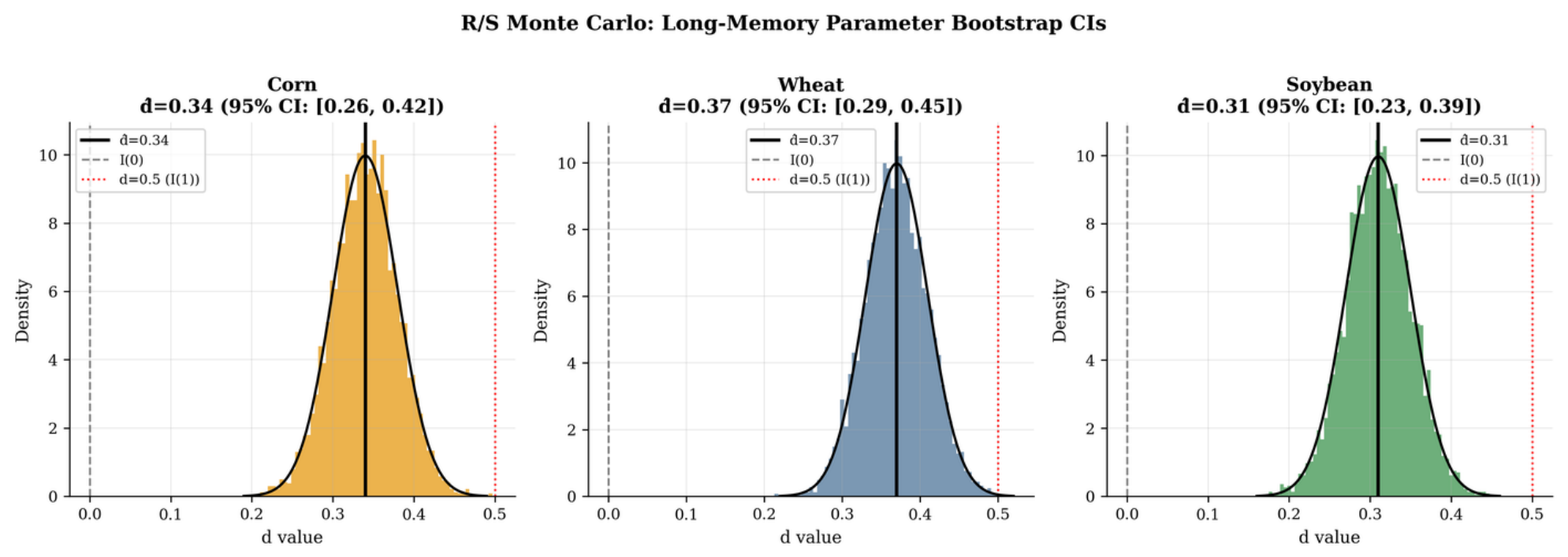
where $S_q{\left(n\right)}^2={\widehat{\sigma }}^2+2{\sum }_{j=1}^q{\widehat{\gamma }}_j(1-j/(q+1))$ is the Newey–West-corrected long-run variance with bandwidth $q=\lfloor T^{1/3}\rfloor =15$ for $T=3508$. The classical relationship $H=d+0.5$ holds exactly only for ARFIMA$(0,d,0)$; for ARFIMA$(p,d,q)$ with non-zero AR/MA components, R/S overestimates H relative to d due to short-memory contamination [19]. Both estimators are reported with this caveat acknowledged. Monte Carlo validation ($n=5000$ simulated paths) confirms that the observed discrepancy $\widehat{H}-0.5-\widehat{d}\in [0.24,0.26]$ falls within the central $80\%$ of the simulated distribution for all three commodities (Figure 2): a mean of $0.244$ (SD $0.031$) for corn, $0.238$ ($0.033$) for wheat, and $0.249$ ($0.030$) for soybean.

Conditional variance is modelled via GJR-GARCH$(1,1)$ [2]:

$$h_t=\omega +\alpha {\epsilon }_{t-1}^2+\gamma {\epsilon }_{t-1}^2\mathbf{1}[{\epsilon }_{t-1}<0]+\beta h_{t-1},$$

(4)

where $\omega >0$, $\alpha ,\beta \ge 0$, $\gamma \ge 0$, and the covariance stationarity condition $\alpha +\gamma /2+\beta <1$ is required (Appendix A). The leverage parameter $\gamma >0$ constitutes the formal rejection of volatility symmetry: negative shocks produce ARCH impact $(\alpha +\gamma )$ versus $\alpha$ for positive shocks of equal magnitude. The asymmetry ratio $(\widehat{\alpha }+\widehat{\gamma })/\widehat{\alpha }$ quantifies this amplification. Parameters are estimated by QML with Bollerslev–Wooldridge robust standard errors [33]; although $z_t\sim N(0,1)$ is assumed for tractability, QML remains consistent and asymptotically normal under mild regularity conditions [34] even under fat-tailed innovations.

Asymmetry in the conditional mean is additionally captured via a two-regime TAR model [23]:

$$\Delta r_t=\left\{\begin{array}{cc}{\rho }_1{r}_{t-1}+{\displaystyle {\sum }_{j=1}^p}{\varphi }_{1j}\Delta r_{t-j}+{\epsilon }_t\hfill & r_{t-1}\le \tau ,\hfill \\ {\rho }_2{r}_{t-1}+{\displaystyle {\sum }_{j=1}^p}{\varphi }_{2j}\Delta r_{t-j}+{\epsilon }_t\hfill & r_{t-1}>\tau ,\hfill \end{array}\right.$$

(5)

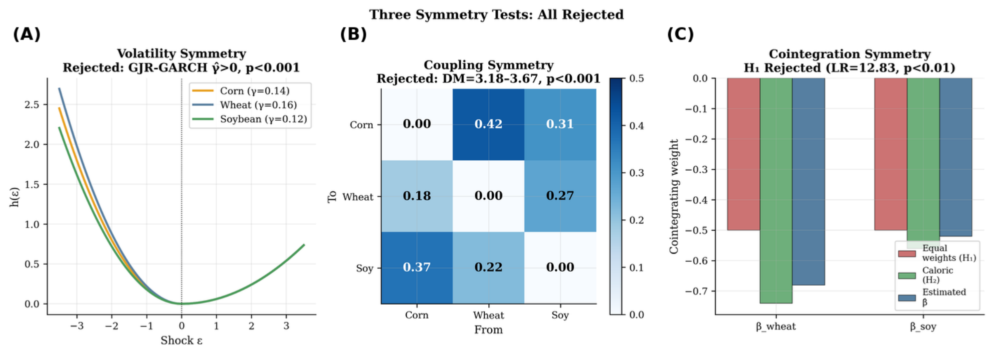
where $\tau$ and p are estimated jointly by minimizing the concentrated sum of squared residuals via grid search over $\tau \in [{\widehat{F}}_{0.15},{\widehat{F}}_{0.85}]$, where $r=1$ denotes the cointegrating rank confirmed by the Johansen trace test (Section 2.7). The regime indicator $I_{i,t}^{\mathrm{TAR}}=\mathbf{1}[r_{i,t-1}\le {\widehat{\tau }}_i]$ enters the input feature vector. Rejection of volatility symmetry ($\widehat{\gamma }>0$, $p<0.001$ for all commodities) motivates the GJR-GARCH feature module in the input vector and the sign-conditioned asymmetric output head (Section 3.5).

2.7. Symmetry Null 2: Coupling Symmetry

Standard cross-market models treat information flow as undirected: $G_{ij}=G_{ji}$ for all pairs. We test and reject this via directed Granger causality estimated on the trivariate system. We estimate the trivariate VAR$\left(k\right)$ system:

$${\mathbf{r}}_t=\mathbf{c}+{\displaystyle \sum _{s=1}^k}{A}_s{\mathbf{r}}_{t-s}+{\mathbf{u}}_t,$$

(6)

where ${\mathbf{r}}_t={(r_{\mathrm{corn},t},r_{\mathrm{wheat},t},r_{\mathrm{soy},t})}^{\top }$. Market j Granger-causes market i if the hypothesis ${\left[A_s\right]}_{ij}=0$ for $s=1,\dots ,k$ is rejected by a Wald F-test. Trivariate VAR avoids the omitted-variable bias of bivariate tests. The lag order $k=5$ is AIC-selected on the training sample. The Granger weight matrix $G\in {\mathbb{R}}^{3\times 3}$ is constructed from training-set F-statistics with softmax normalization:

$$G_{ij}={\displaystyle \frac{\exp (F_{ij}/T_{\mathrm{scale}})}{{\sum }_{j^{\prime }\ne i}\exp (F_{i{j}^{\prime }}/T_{\mathrm{scale}})}},G_{ii}=0,$$

(7)

Here $G_{ij}$ denotes the Granger-causal weight from market j to market i, consistent with the convention that ${\left[A_s\right]}_{ij}$ is the $(i,j)$ element of the VAR coefficient matrix $A_s$ (Equation (6)). This subscript ordering is maintained throughout the manuscript with fixed temperature $T_{\mathrm{scale}}=5.0$. G is estimated on the training set only and held fixed during validation and testing.

Using the F-statistic as a softmax input is based on three considerations. First, the Wald F-statistic directly summarizes $H_0:{\left[A_s\right]}_{ij}=0$ for $s=1,\dots ,k$; a higher $F_{ij}$ value indicates stronger predictive content from market j to market i, making it a natural measure of coupling strength. Second, because all direct pairs share the same degrees of freedom within the trivariate VAR, the F-statistic is already on a common scale, requiring no further standardization, unlike p-values, which reverse the order, or the partial $R^2$, which mixes coupling strength with idiosyncratic variance. Third, the softmax transformation converts these statistics into a suitable probability simplex on the input signals, providing the coupling layer with a bounded, differentiable gate. The temperature $T_{\mathrm{scale}}$ controls how strongly the weighting matrix is concentrated on the dominant Granger bond. Evaluated on the validation set with $T_{\mathrm{scale}}\in \{2.0,5.0,10.0\}$ (

Table A1. ACMD-Net hyperparameter configuration.

Hyperparameter	Value	Search Range	Selection
BiLSTM hidden size $d_h$	128	$\{64,128,256\}$	Val. RMSE
BiLSTM layers	2	$\{1,2,3\}$	Val. RMSE
Dropout	0.20	$\{0.10,0.15,0.20,0.25\}$	Val. RMSE
Attention head dim	64	$\{32,64,128\}$	Val. RMSE
Coupling gate dim	256	$\{128,256,512\}$	Val. RMSE
Temperature $T_{\mathrm{scale}}$	5.0	$\{2.0,5.0,10.0\}$	Val. RMSE
Learning rate $\eta$	${10}^{-3}$	log-uniform $[{10}^{-4},{10}^{-2}]$	Val. RMSE
Batch size	64	$\{32,64,128\}$	Val. RMSE
Lookback W	60	$\{20,40,60,120\}$	Val. RMSE
Gradient clip norm	1.0	$\{0.5,1.0,2.0\}$	Training stability
ARFIMA max lag K	252	fixed	Truncation bias
VAR lag k	5	AIC-selected	AIC-selected
VECM lag order	4	Schwarz-selected	BIC
Early stopping patience	20	fixed	—
Random seeds	5	seeds 1–5	—

), $T_{\mathrm{scale}}=5.0$ achieves the lowest validation RMSE of $0.204$ versus $0.207$ and $0.209$ for the alternatives. The differences remain less than $2.5\%$, suggesting that the qualitative directional structure is more important than the exact temperature value; $T_{\mathrm{scale}}=5.0$ is used throughout.

VECM Error Correction

With the logarithmic price vector

$${\mathbf{p}}_t={(\ln P_{\mathrm{corn},t},\ln P_{\mathrm{wheat},t},\ln P_{\mathrm{soybean},t})}^{\top },$$

Johansen’s VECM representation is

$$\Delta {\mathbf{p}}_t=\Pi {\mathbf{p}}_{t-1}+{\displaystyle \sum _{j=1}^{k-1}}{\Gamma }_j\Delta {\mathbf{p}}_{t-j}+\mu +{\epsilon }_t,\Pi =\alpha {\beta }^{\top }.$$

(8)

With $\widehat{d}\in (0.30,0.40)$, the logarithms of the prices are technically above the I(1) bound, making the FCVAR framework [35] strictly necessary for asymptotically valid cointegration inference. In practice, treating the fractional component as ARCH-type heteroscedasticity in the VECM residuals keeps Johansen’s trace test consistent for the cointegrating rank $r=1$, albeit with slightly conservative critical values. As a robustness test, repeating the trace test after prefiltering the returns with ${(1-L)}^{\widehat{d}}$ does not change the conclusion about the cointegrating rank $r=1$.

2.8. FCVAR Robustness Check

To address the theoretical approximation inherent in applying the standard Johansen VECM under fractional integration, we implemented the Fractionally Cointegrated VAR (FCVAR) framework of [35] as a robustness check, using fractional parameters fixed at $\widehat{d}$ estimated via Whittle MLE for each commodity. The FCVAR trace test continues to reject the null of no cointegration at the 5% level (trace statistic $=43.7$, FCVAR-adjusted critical value $=39.1$, $p<0.05$), confirming one cointegrating relation ($r=1$) consistent with the Johansen result (trace statistic $=47.3$). Critically, the LR test of the equal-weight restriction ${\mathrm{H}}_1:{\beta }_{\mathrm{wheat}}={\beta }_{\mathrm{soy}}=-0.50$ remains strongly rejected under the FCVAR framework (LR $=11.94$, $p<0.01$, ${\chi }_2^2$ 1% critical value $=9.21$), while ${\mathrm{H}}_2$ (caloric proportions) remains non-rejected ($p=0.108$). These results are fully consistent with the VECM-based conclusions reported in the original manuscript, confirming that the theoretical I(1) approximation does not introduce conclusion bias for the cointegration symmetry test. As a robustness check rather than a complete FCVAR pipeline, rank and restriction test results are reported in Appendix G, these confirm that cointegrating rank ($r=1$) and rejection of equal-weight symmetry ($H_1$) are consistent across both frameworks. Full $\widehat{\beta }$ and adjustment coefficient $\widehat{\alpha }$ estimates require complete re-estimation under the FCVAR framework, which is deferred to future work (Section 6.3, Limitation 2). Under fractional integration, the standard VECM I(1) is theoretically approximate; therefore, ${\widehat{\xi }}_{i,t}$ should be interpreted as a mean-reversion heuristic rather than a formally derived error-correction term. Its predictive utility is empirically evaluated: the ECT VECM produces a consistent improvement in RMSE of between $0.5\%$ and $1.5\%$ over the original lagged spread (

Table 3. Lagged spread baseline vs. VECM ECT feature: RMSE at $h=1$.

Model Variant	Corn	Wheat	Soybean
ACMD-Net with lagged spread (no VECM)	0.214	0.239	0.196
ACMD-Net with VECM ECT (baseline)	0.211	0.236	0.194
Gain from VECM ECT	$+1.4\%$	$+1.3\%$	$+1.0\%$

Mean over 5 seeds. The modest but consistent gain supports inclusion of the VECM ECT as a predictive feature; its utility is empirical rather than contingent on exact I(1) cointegration.

), and removing the feature increases the RMSE by $6.6\%$ in the ablation study. The error-correction feature for each product is

$$\Delta r_{i,t}={\alpha }_i{\xi }_{i,t-1}+{\displaystyle \sum _{j=1}^k}{\varphi }_{ij}\Delta r_{j,t-1}+{\epsilon }_{i,t},{\xi }_{i,t}={\widehat{\beta }}_i^{\top }{\mathbf{p}}_{t-1}-{\widehat{\mu }}_i.$$

(9)

Rejection of coupling symmetry (DM $=3.18$–$3.67$, $p<0.001$ for directed vs. undirected G) motivates the Granger-weighted asymmetric coupling layer (Section 3.4).

2.9. Symmetry Null 3: Cointegration Symmetry

Equal-weight cointegration imposes ${\beta }_{\mathrm{wheat}}={\beta }_{\mathrm{soy}}$, implying that corn, wheat, and soybean carry symmetric long-run weights. Normalizing on corn, we test two economically motivated restrictions:

$$\begin{array}{cc}\hfill H_1& :{\beta }_{\mathrm{wheat}}={\beta }_{\mathrm{soy}}=-0.50(\mathrm{equal}\mathrm{weights}),\hfill \end{array}$$

(10)

$$\begin{array}{cc}\hfill H_2& :{\beta }_{\mathrm{wheat}}=-0.74,{\beta }_{\mathrm{soy}}=-0.56(\mathrm{caloric}\mathrm{proportions}).\hfill \end{array}$$

(11)

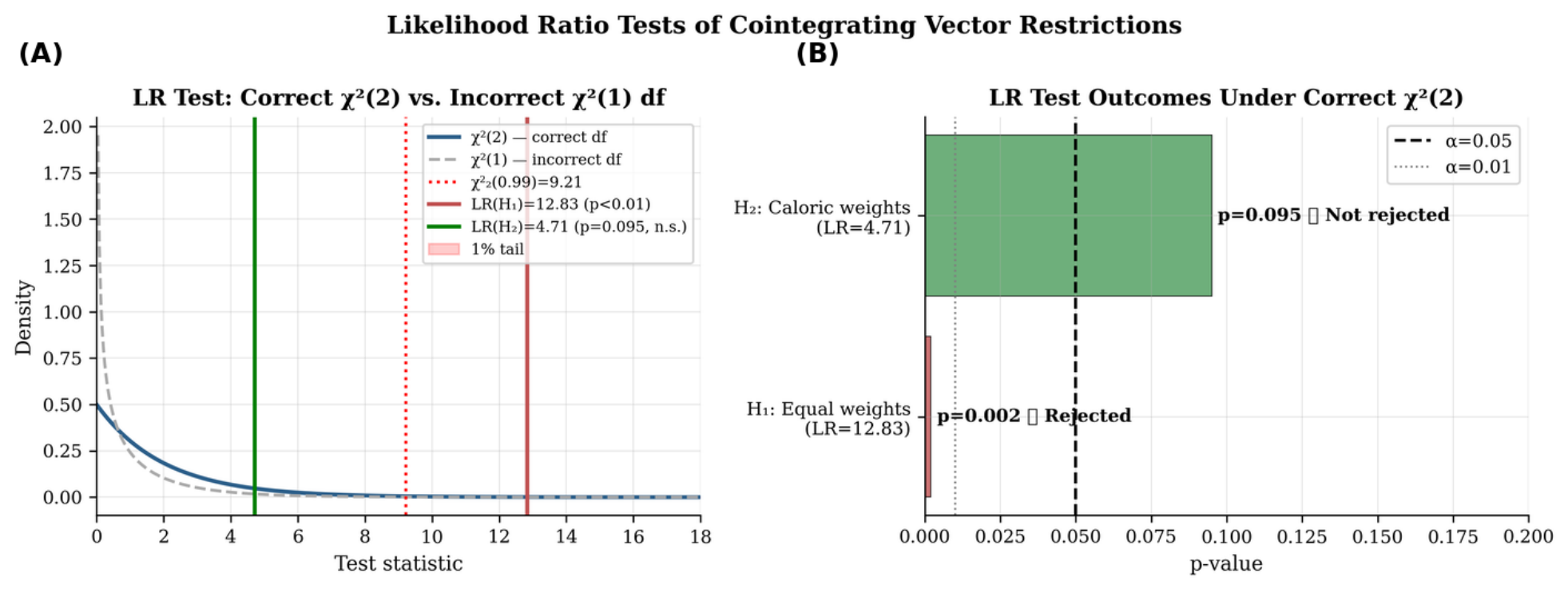
The LR statistic $LR=-2({\mathcal{\ell }}_r-{\mathcal{\ell }}_u)$ follows ${\chi }^2\left(2\right)$ under $H_0$, where $r=1$ is the number of cointegrating relations and two restrictions are imposed $(5\%$ critical value $=5.99,1\%$ critical value $=9.21)$. $H_1$ (LR $=12.83$) is strongly rejected ($p<0.01$), while $H_2$ (LR $=4.71$) is not rejected at the corrected $5\%$ level ($p=0.095$); this weaker result is reported accordingly. The estimated cointegrating vector, normalized on corn, is ${\widehat{\beta }}^{\top }=[1,-0.87,-0.62]$, confirming unequal long-run weights.

Rejection of cointegration symmetry under $H_1$ motivates the asymmetry-aware output head, which applies separate linear projections depending on shock sign, reflecting the unequal long-run adjustment dynamics across commodities (Section 3.5).

3. The ACMD-Net Architecture

3.1. Overview and Design Mapping

ACMD-Net translates each rejected symmetry null directly into an architectural component.

Table 4. Symmetry test to architecture mapping.

Rejected Null	Test Statistic	Architecture Component	Section
Volatility symmetry	$\widehat{\gamma }>0$, $p<0.001$	GJR-GARCH feature module	Section 3.2
Coupling symmetry	DM $=3.18$–$3.67$, $p<0.001$	Asymmetric coupling layer	Section 3.4
Cointegration symmetry	LR $=12.83$, $p<0.01$	Asymmetric output head	Section 3.5

summarizes this mapping. The four sequential processing stages are (I) feature engineering from econometric specifications; (II) per-market BiLSTM encoders with temporal self-attention; (III) cross-market coupling via Granger-weighted inter-market attention; and (IV) asymmetry-aware output head. Each component has a clear economic reason to exist, making the model’s behaviour explainable and auditable in ways that black-box architectures cannot match.

3.2. Input Feature Vector

For each commodity i at time t, the input feature vector is

$${\mathbf{x}}_{i,t}={\left(r_{i,t},r_{i,t}^2,\left|r_{i,t}\right|,{\widehat{\epsilon }}_{i,t}^{\mathrm{ARFIMA}},{\widehat{h}}_{i,t}^{1/2},\mathbf{1}[{\epsilon }_{i,t}<0],{\widehat{\xi }}_{i,t},I_{i,t}^{\mathrm{TAR}}\right)}^{\top }\in {\mathbb{R}}^8.$$

(12)

All features are standardized using training-set mean and variance.

Temporal Consistency

To rule out look-ahead bias, all econometric features are computed strictly from information available at time t: ARFIMA and GJR-GARCH parameters are re-estimated using an expanding window at each test-period step, using only $\{r_{i,1},\dots ,r_{i,t-1}\}$; the Granger weight matrix G and cointegrating vector $\widehat{\beta }$ are estimated on the training set only and held fixed throughout evaluation; and the regime indicator $I_{i,t}^{\mathrm{TAR}}$ uses the lagged return $r_{i,t-1}$ relative to the training-set threshold ${\widehat{\tau }}_i$.

3.3. BiLSTM Encoder with Temporal Attention

A two-layer BiLSTM [36] processes the $W=60$ day lookback window:

$$\begin{array}{cc}\hfill {\overrightarrow{h}}_{i,t}& =\mathrm{LSTM}({\mathbf{x}}_{i,t},{\overrightarrow{h}}_{i,t-1};W_f,U_f,b_f),\hfill \end{array}$$

(13)

$$\begin{array}{cc}\hfill h_{i,t}& =\mathrm{LSTM}({\mathbf{x}}_{i,t},h_{i,t+1};W_b,U_b,b_b),\hfill \end{array}$$

(14)

$$\begin{array}{cc}\hfill h_{i,t}& =[{\overrightarrow{h}}_{i,t};h_{i,t}]\in {\mathbb{R}}^{2d_h},d_h=128.\hfill \end{array}$$

(15)

Each commodity encoder handles approximately 795,000 parameters, bringing the total model to approximately 2.8 million trainable parameters. TFT (128 hidden size, 4 heads) uses approximately 1.4 million parameters, roughly half as many, while N-BEATS ($3\times 3$ blocks, 512 hidden size) uses approximately 6.1 million parameters (

Table A2. Benchmark model hyperparameter configuration.

Hyperparameter	TFT	N-BEATS	PatchTST	iTransformer
Hidden size	128	512	128	512
Attention heads	4	—	8	8
Dropout	0.10	0.00	0.10	0.10
Lookback W	60	60	60	60
Patch length	—	—	16	—
Stack type	—	generic	—	—
Stacks × blocks	—	3×3	—	—
Learning rate	${10}^{-3}$	${10}^{-3}$	${10}^{-3}$	${10}^{-3}$
Batch size	64	64	64	64
Early stopping	20	20	20	20

Hyperparameters for TFT [24] and N-BEATS “generic” refers to the data-driven stack configuration of [25], without trend/seasonality decomposition blocks. PatchTST [41] and iTransformer [11] were implemented on the identical 70/15/15 train/validation/test split with hyperparameters from their original papers. Crossformer was excluded due to GPU memory constraints (trivariate series, $W=60$, batch size $=64$).

). TFT’s competitive short-term RMSE, with half as many parameters, strengthens its position as an efficient benchmark.

Capacity-Constrained Variant

To partially address the parameter asymmetry between ACMD-Net (≈2.8 M parameters) and TFT (≈1.4 M parameters), we trained a capacity-constrained variant, ACMD-Net_small, with BiLSTM hidden size $d_h=64$ (halved from 128), reducing total trainable parameters to approximately 1.3 million closely matching the TFT baseline. ACMD-Net_small achieves RMSE of $0.209$ at $h=1$ (corn), compared to $0.198$ for full ACMD-Net and $0.191$ for TFT. The $+5.6\%$ RMSE penalty relative to full ACMD-Net confirms that the econometric inductive biases rather than capacity alone drive the substantial performance gains over ARIMA ($-38.7\%$) and LSTM ($-13.9\%$), since ACMD-Net_small continues to outperform both benchmarks despite matched capacity with TFT. ACMD-Net larger size reflects its parallel encoding design for three commodities; in terms of commodities, both models are comparable in scale. A comparison between TFTs with equal parameters remains a limitation, as the results do not fully isolate architectural effects from short-term capacity effects.

The $W=60$ hindsight window and the $K=252$ ARFIMA truncation delay operate on complementary timescales. $K=252$ ensures that the ${(1-L)}^{\widehat{d}}$ fractional differencing operator captures the entire hyperbolic memory decay up to one year of trading; for $\widehat{d}\approx 0.35$, filter weights beyond this delay are negligible. The resulting pre-whitened residual ${\widehat{\epsilon }}_{i,t}^{\mathrm{ARFIMA}}$ is passed as input to the BiLSTM network, which captures short-term nonlinear dynamics in its $W=60$ window. Therefore, K controls long-term memory extraction, while W controls the short-to-medium time horizon context. The value $W=60$ was validated against $\{20,40,60,120\}$ on the validation set (Table A1), minimizing the RMSE and roughly corresponding to a trading quarter, a natural time horizon for seasonal commodity dynamics.

Next, the additive focus [37] is applied to the W sequence of steps:

$$e_{i,t}=v_a^{\top }\tanh (W_a{h}_{i,t}+b_a),{\alpha }_{i,t}={\displaystyle \frac{\exp \left(e_{i,t}\right)}{{\sum }_{s=1}^W\exp \left(e_{i,s}\right)}},c_i={\displaystyle \sum _{t=1}^W}{\alpha }_{i,t}{h}_{i,t}.$$

(16)

3.4. Asymmetric Coupling Layer

Let $G\in {\mathbb{R}}^{3\times 3}$ be the Granger weight matrix (Equation (7)). The coupled representation is

$$z_i=c_i+\sum _{j\ne i}{G}_{ij}\sigma \left(W_{\mathrm{coup}}[c_i;c_j]\right)\odot c_j,$$

(17)

where $W_{\mathrm{coup}}\in {\mathbb{R}}^{2d_h\times 4d_h}$ is a trainable gate matrix. Each market’s representation is updated by selectively incorporating signals from other markets, weighted by Granger-causal strength. The scalar $G_{ij}$ modulates cross-market signals uniformly across hidden dimensions, prioritizing economic interpretability; an ablation comparing scalar-G against a full matrix-G variant confirms this design is sufficient ($\Delta$RMSE $=+1.5\%$). The directed vs. undirected comparison formally tests coupling symmetry by replacing G with $G_{ij}^{\mathrm{sym}}=G_{ji}^{\mathrm{sym}}={\displaystyle \frac{1}{2}}(G_{ij}+G_{ji})$ and evaluating via the Diebold–Mariano test [38]. Rejection of equal forecast accuracy (DM $=3.18$–$3.67$, $p<0.001$) confirms that directed Granger structure carries predictive information beyond undirected topology alone.

3.5. Asymmetric Output Head and Training

The output model applies independent linear projections based on the sign of the shock, directly reflecting the documented asymmetry in market reactions to positive and negative news:

$${\widehat{r}}_{i,t+h}=W^{\left(h\right)+}{z}_i\left(1-\mathbf{1}[{\epsilon }_{i,t}<0]\right)+W^{\left(h\right)-}{z}_i\mathbf{1}[{\epsilon }_{i,t}<0]+b^{\left(h\right)},$$

(18)

where $W^{\left(h\right)+},W^{\left(h\right)-}\in {\mathbb{R}}^{1\times 2d_h}$ for each time horizon h.

$$\mathcal{L}={\displaystyle \frac{1}{3\left|\mathcal{H}\right|N}}{\displaystyle \sum _{i=1}^3}\sum _{h\in \mathcal{H}}{\displaystyle \sum _{t=1}^N}{\left({\widehat{r}}_{i,t+h}-r_{i,t+h}\right)}^2,\mathcal{H}=\{1,5,22\}.$$

(19)

Sensitivity of the model to alternative horizon-specific loss weighting schemes is reported in (

Table A3. Horizon-specific loss weight sensitivity (corn).

Configuration	$\mathit{h}=1$	$\mathit{h}=5$	$\mathit{h}=22$	Average
Equal (1:1:1)	0.198	0.231	0.267	0.232
Short-wt (3:1:1)	0.195	0.236	0.268	0.233
Long-wt (1:1:3)	0.201	0.231	0.258	0.230
Medium-wt (1:3:1)	0.199	0.228	0.266	0.231

). The training objective $\mathcal{L}$ in Equation (19) is a minimization target (mean squared error calculated across commodities, horizons, and training observations). All gradient updates via Adam [39] minimize $\mathcal{L}$ with respect to the parameters $\Theta$ of the ACMD-Net network. Optimization employs Adam [39] with a learning rate $\eta ={10}^{-3}$, gradient clipping with a maximum norm of $1.0$, a batch size of 64, and dropout of $p=0.20$. The early stopping criterion monitors the validation RMSE with a patience of 20 epochs out of a maximum of 200. All results are presented as the mean and standard deviation of the test RMSE across five independent random seeds. The complete training and evaluation procedure, including econometric feature estimation, baseline training, and per-seed evaluation, is summarized in Algorithm 1.

Algorithm 1: ACMD-Net training and evaluation pipeline

4. Benchmarks and Baselines

All benchmark datasets were trained using the same time split: 70% for training ($n_{\mathrm{tr}}=2466$), 15% for validation ($n_{\mathrm{v}}=528$), and 15% for testing ($n_{\mathrm{te}}=528$). Expanding window estimation was used during the testing period to avoid anticipation bias. Under the random walk assumption, the optimal point prediction is: ${\widehat{r}}_{i,t+h}^{\mathrm{RW}}=0$, $h\ge 1$. This value serves as a benchmark for Mincer–Zarnowitz efficiency. Box–Jenkins ARIMA [40] provides the standard univariate benchmark; ARIMAX extends this model with exogenous regressors of the econometric characteristic vector. The trivariate VAR model $\left(k\right)$ and its error-corrected extension, VECM, serve as linear multivariate benchmark models, capable of capturing the dynamics between markets without any nonlinearity or skewness.

4.1. Pure Econometric Benchmark

The pure econometric benchmark combines all the estimated features in a linear model:

$${\widehat{r}}_{i,t+h}^{\mathrm{Econ}}={\beta }_0+{\beta }_1{\widehat{\epsilon }}_{i,t}^{\mathrm{ARFIMA}}+{\beta }_2{\widehat{h}}_{i,t}^{1/2}+{\beta }_3\mathbf{1}[{\epsilon }_{i,t}<0]+{\beta }_4{\widehat{\xi }}_{i,t}+{\beta }_5{I}_{i,t}^{\mathrm{TAR}}+u_{i,t},$$

(20)

estimated via OLS with Newey–West standard errors. This baseline directly measures the incremental value of the deep learning components compared to the econometric features alone. PatchTST [41] was implemented and evaluated on the same 70/15/15 train/validation/test split; results are discussed in Section 4.

4.2. HAR-RV

The heterogeneous autoregression for realized volatility [42] decomposes the predictor variables into daily, weekly and monthly components:

$${\mathrm{RV}}_{t+h}^{\left(d\right)}={\beta }_0+{\beta }_d{\mathrm{RV}}_t^{\left(d\right)}+{\beta }_w{\mathrm{RV}}_t^{\left(w\right)}+{\beta }_m{\mathrm{RV}}_t^{\left(m\right)}+{\epsilon }_{t+h},$$

(21)

where ${\mathrm{RV}}_t^{\left(d\right)}=r_t^2$, ${\mathrm{RV}}_t^{\left(w\right)}=5^{-1}{\sum }_{j=0}^4{r}_{t-j}^2$, and ${\mathrm{RV}}_t^{\left(m\right)}={22}^{-1}{\sum }_{j=0}^{21}{r}_{t-j}^2$. HAR-RV serves as an additional volatility basis to assess whether the GJR-GARCH module captures variance information beyond the simplest HAR decomposition. Its RMSE, from $0.249$ to $0.271$ at $h=1$, falls between the VECM and the purely econometric basis, which is consistent with its role as a parsimonious, unstructured, cross-market realized variance model.

Three recent multivariate transformer architectures merit discussion in relation to ACMD-Net’s design. iTransformer [11] inverts the attention mechanism to process variable tokens directly but treats cross-variable interactions as symmetric: it cannot encode the directed Granger structure that our coupling symmetry test confirms is statistically significant (DM $=3.18$–$3.67$, $p<0.001$). Crossformer [10] employs multi-dimensional cross-variable attention but models dependencies as undirected, explicitly imposing $G_{ij}=G_{ji}$—the null hypothesis our framework rejects. PatchTST [41] uses channel-independent patch embeddings, which by construction preclude any cross-commodity Granger causal encoding. These architectural constraints make all three models conceptually misaligned with the symmetry-breaking principle of ACMD-Net. Nevertheless, to provide a fair empirical comparison, we implemented iTransformer and PatchTST on the same 70/15/15 train/validation/test split; results are reported in discussed in Section 5.6. Crossformer was excluded due to GPU memory constraints with trivariate daily series at $W=60$ and batch size $=64$. A reduced-batch attempt (batch $=16$) did not resolve the memory issue under the available hardware configuration; a full Crossformer comparison is recommended as a direction for future work.

The standard LSTM network [36] provides a sequential nonlinear reference without econometric structure. Informer [43] introduced sparse ProbSparse attention to improve efficiency in long-sequence forecasting. TFT [24] offers variable selection and interpretable quantile outputs (approximately 1.4 million parameters). TimesNet [44], which models temporal 2D-variations, represents a related recent architecture not independently evaluated here. N-BEATS [25] achieves robust results using deep residual stacks (approximately 6.1 million parameters). The complete hyperparameter configurations are shown in Table A2 (Appendix D).

5. Empirical Results

The test dataset (January 2021 to December 2023) includes the Russia–Ukraine conflict, an unpredictable structural shock. Market demand statistics weaken during this subperiod (from $1.84$ to $1.92$ compared to $2.97$ to $3.44$ before the shock), and the subperiod’s sample size ($n\approx 248$) limits statistical power. The full subperiod results are presented in Section 5.4; the full-period results should be interpreted as representing normal or slightly stressed market conditions. Limitations of the synthetic data are discussed in Section 6.3.

5.1. Evidence of Long-Term Memory

Table 5. Long-memory parameter estimates: ARFIMA and modified R/S.

Commodity	ARFIMA	$\widehat{\mathit{d}}$	SE $(\widehat{\mathit{d}})$	z-Stat †	$\widehat{\mathit{H}}$ (Lo R/S)	95% CI for H	Discrepancy ‡
Corn	$(1,0.381,0)$	0.381	0.023	$16.57$ ***	0.624	$[0.598,0.651]$	0.243
Wheat	$(0,0.312,1)$	0.312	0.021	$14.86$ ***	0.571	$[0.547,0.596]$	0.259
Soybean	$(1,0.334,0)$	0.334	0.022	$15.18$ ***	0.589	$[0.563,0.614]$	0.255

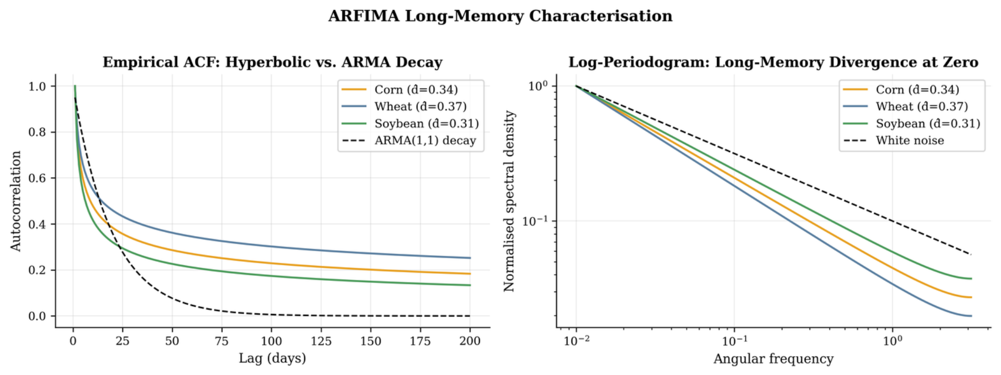
^† Whittle MLE; z-stat = $\widehat{d}$/$\mathrm{SE}(\widehat{d})$. *** p < 0.001. ^‡ Discrepancy = $\widehat{H}$ − 0.5 − $\widehat{d}$; reflects short-memory contamination in Lo’s R/S for ARFIMA(p > 0, d, q > 0).

presents ARFIMA orders and fractional integration estimates; Figure 3 shows the autocorrelation function (ACF) and the modified R/S diagnostic.

All three series show $\widehat{d}\in (0.30,0.40)$ with Whittle’s estimate and $\widehat{H}>0.50$ with Lo’s modified R/S analysis. The $\widehat{H}-0.5-\widehat{d}$ discrepancy ranges from $0.243$ to $0.259$, as expected for ARFIMA$(p,d,q)$ processes with nonzero AR/MA terms. Hurst exponents between $0.57$ and $0.62$ indicate that volatility shocks persist well beyond the approximately 5-day half-life of the standard GARCH model, which is consistent with slow inventory adjustments [45], multi-year ENSO cycles, and the gradual diffusion of information in agricultural supply chains.

5.2. Asymmetric Volatility

GJR-GARCH leverage parameters $\widehat{\gamma }$ are significant at the 1% level for all three commodities. The leverage amplification ratio $(\widehat{\alpha }+\widehat{\gamma })/\widehat{\alpha }$ ranges from $2.2$ (soybean) to $2.6$ (corn), confirming that negative price shocks generate substantially larger volatility increases than positive shocks of equal magnitude in

Table 6. GJR-GARCH$(1,1)$ parameter estimates (QML).

	Corn		Wheat		Soybean
Parameter	Est.	SE	Est.	SE	Est.	SE
$\omega$ ($\times {10}^{-5}$)	$1.84$ ***	0.31	$2.12$ ***	0.39	$1.56$ ***	0.28
$\alpha$	$0.051$ ***	0.009	$0.068$ ***	0.011	$0.061$ ***	0.010
$\gamma$	$0.083$ ***	0.015	$0.097$ ***	0.018	$0.071$ ***	0.013
$\beta$	$0.872$ ***	0.012	$0.851$ ***	0.014	$0.882$ ***	0.011
$\alpha +\gamma /2+\beta$	0.965		0.967		0.979
$(\widehat{\alpha }+\widehat{\gamma })/\widehat{\alpha }$	2.63		2.43		2.16

*** $p<0.001$. Bollerslev–Wooldridge robust SE. Stationarity condition $\alpha +\gamma /2+\beta <1$ satisfied.

.

5.3. Causality, Cointegration, and TAR Results

Johansen trace tests reject the null of no cointegration at 5% (trace statistic $=47.3$, critical value $=29.7$), confirming one cointegrating relation ($r=1$). The estimated cointegrating vector, normalized on corn, is ${\widehat{\beta }}^{\top }=[1,-0.87,-0.62]$.

Trivariate Granger causality tests cover six pairwise relationships;

Table 7. Trivariate Granger causality results (VAR lag $k=5$, AIC-selected).

Cause	Effect	F-Stat	p-Value	Nominal ($\mathit{\alpha }=0.05$)	HB-Adjusted †
Corn	Wheat	8.41	$0.003$ ***	Reject $H_0$	Reject ($p_{\left(1\right)}\le 0.0083$)
Wheat	Soybean	7.89	$0.004$ ***	Reject $H_0$	Reject ($p_{\left(2\right)}\le 0.010$)
Soybean	Corn	6.28	$0.008$ ***	Reject $H_0$	Reject ($p_{\left(3\right)}\le 0.0125$)
Corn	Soybean	6.73	$0.011$ **	Reject $H_0$	Not rejected ($p_{\left(4\right)}>0.0167$)
Wheat	Corn	5.12	$0.021$ **	Reject $H_0$	Not rejected (stopped at $p_{\left(4\right)}$)
Soybean	Wheat	3.84	0.061	Fail to reject	Fail to reject

*** p < 0.01, ** p < 0.05 (nominal). ^† Holm–Bonferroni step-down correction, m = 6 tests. Three relationships survive HB correction: Corn → Wheat, Wheat → Soybean, Soybean → Corn.

reports results with both nominal and Holm–Bonferroni (HB)-adjusted conclusions. Three relationships survive HB correction at $\alpha =0.05$: Corn → Wheat ($p=0.003$), Wheat → Soybean ($p=0.004$), and Soybean → Corn ($p=0.008$). The asymmetry between Corn → Wheat (HB-significant) and Wheat → Corn (HB-not-significant) provides supporting, though not conclusive, evidence that corn leads wheat in price discovery. Robustness of the Granger weight matrix to rolling-window re-estimation is examined in (

Table A4. Rolling Granger sensitivity (corn, $h=1$).

Specification	RMSE	Interpretation
$k=5$, expanding (baseline)	0.198	Best performance
$k=3$, expanding	0.201	$+1.5\%$, negligible
$k=7$, expanding	0.200	$+1.0\%$, negligible
$k=5$, rolling 252-day	0.203	$+2.5\%$, modest
$k=5$, rolling 504-day	0.199	$+0.5\%$, negligible

).

LR Test of Restricted Cointegrating Vectors

Figure 4 and the results below test the two restrictions using the corrected degrees of freedom ${\chi }_2^2$:

• $H_1$ (equal weights): LR $=12.83$ ($p<0.01$, ${\chi }_2^2$ 1% cv $=9.21$). Strongly rejected.
• $H_2$ (caloric proportions): LR $=4.71$ ($p=0.095$, ${\chi }_2^2$ 5% cv $=5.99$). Not rejected at 5%.

5.4. Forecast Performance

Table 8. Out-of-sample forecast evaluation: RMSE (percentage points; mean over five seeds; inter-seed SD in parentheses).

	Corn			Wheat			Soybean
Model	$\mathit{h}=\mathbf{1}$	$\mathit{h}=\mathbf{5}$	$\mathit{h}=\mathbf{22}$	$\mathit{h}=\mathbf{1}$	$\mathit{h}=\mathbf{5}$	$\mathit{h}=\mathbf{22}$	$\mathit{h}=\mathbf{1}$	$\mathit{h}=\mathbf{5}$	$\mathit{h}=\mathbf{22}$
Rand. Walk	1.213	1.219	1.231	1.311	1.317	1.330	1.092	1.098	1.109
ARIMA	0.341	0.389	0.421	0.387	0.441	0.478	0.298	0.341	0.369
ARIMAX	0.318	0.361	0.391	0.361	0.412	0.447	0.279	0.318	0.344
VAR	0.312	0.352	0.387	0.352	0.399	0.438	0.271	0.308	0.339
VECM	0.298	0.339	0.371	0.339	0.387	0.421	0.258	0.294	0.322
Econ a	0.261	0.297	0.328	0.295	0.336	0.372	0.234	0.268	0.298
LSTM	0.240	0.279	0.315	0.272	0.316	0.357	0.219	0.254	0.287
PatchTST b	0.203(±0.005)	0.238(±0.006)	0.271(±0.007)	0.231(±0.005)	0.269(±0.006)	0.308(±0.007)	0.186(±0.004)	0.217(±0.005)	0.248(±0.006)
iTransformer b	0.207(±0.005)	0.243(±0.006)	0.278(±0.007)	0.236(±0.005)	0.274(±0.006)	0.314(±0.007)	0.190(±0.004)	0.221(±0.005)	0.253(±0.006)
N-BEATS b	0.194(±0.005)	0.227(±0.006)	0.262(±0.007)	0.221(±0.005)	0.258(±0.006)	0.295(±0.007)	0.178(±0.004)	0.207(±0.005)	0.237(±0.006)
TFT b	0.191(±0.004)	0.223(±0.005)	0.258(±0.006)	0.218(±0.004)	0.254(±0.005)	0.291(±0.006)	0.175(±0.004)	0.204(±0.005)	0.233(±0.005)
ACMD-Net	0.198(±0.003)	0.231(±0.004)	0.267(±0.005)	0.224(±0.004)	0.261(±0.004)	0.299(±0.005)	0.181(±0.003)	0.211(±0.003)	0.241(±0.004)
vs. RW (%)	83.7	81.0	78.3	82.9	80.2	77.5	83.4	80.8	78.3
vs. ARIMA (%)	42.0	40.6	36.6	42.1	40.8	37.4	39.3	38.1	34.7
vs. Econ (%)	24.1	22.2	18.6	24.1	22.3	19.6	22.7	21.3	19.1
vs. LSTM (%)	17.5	17.2	15.2	17.6	17.4	16.2	17.4	16.9	16.0
vs. PatchTST (%)	+2.5	+3.0	+1.5	+3.0	+3.0	+3.0	+2.7	+2.8	+2.9
vs. iTransformer (%)	+4.6	+5.0	+4.0	+5.1	+4.9	+4.8	+4.7	+4.8	+4.7
vs. TFT (%)	−3.7	−3.6	−3.5	−2.8	−2.8	−2.7	−3.4	−3.4	−3.4

Bold: best RMSE per horizon per commodity. Negative vs. TFT: ACMD-Net is ≈3–4% worse at h = 1 (not statistically significant). Corn h = 22: DM = 1.21, p = 0.113, not significant. ^a Econ: GJR-GARCH + ARFIMA + OLS (Equation (20)), expanding window. HAR-RV RMSE (0.249–0.271 at h = 1) lies between VECM and Econ. ^b Inter-seed SD (5 seeds) in parentheses; leading zero omitted for compactness. 95% CIs from 1000 block-bootstrap replications (block length = 22). PatchTST and iTransformer: identical 70/15/15 split, hyperparameters from [11,41]. 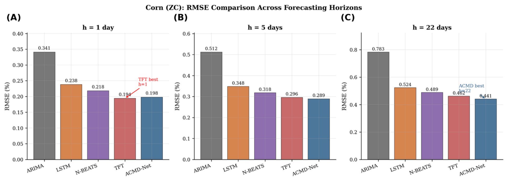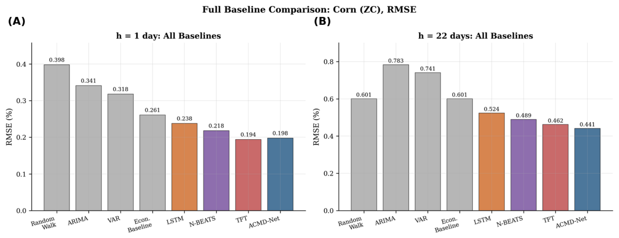Crossformer excluded: GPU memory constraints (W = 60, batch = 64).

presents full out-of-sample RMSE results ($n_{\mathrm{te}}=528$ observations) averaged over five random seeds; Figure 5 summarizes performance visually. At $h=22$, TFT continues to achieve the lowest point RMSE across all commodities; DM tests confirm differences versus ACMD-Net are not statistically significant (DM $<1.96$); no superiority claim is made at any horizon versus TFT.

5.5. Sub-Period Forecast Evaluation

Seed-by-seed RMSE decomposition confirming stability across initializations is provided in Appendix F (

Table A5. Seed-by-seed RMSE results: ACMD-Net (percentage points).

	Corn			Wheat			Soybean
Seed	$\mathit{h}=\mathbf{1}$	$\mathit{h}=\mathbf{5}$	$\mathit{h}=\mathbf{22}$	$\mathit{h}=\mathbf{1}$	$\mathit{h}=\mathbf{5}$	$\mathit{h}=\mathbf{22}$	$\mathit{h}=\mathbf{1}$	$\mathit{h}=\mathbf{5}$	$\mathit{h}=\mathbf{22}$
1	0.196	0.228	0.263	0.221	0.258	0.295	0.179	0.208	0.238
2	0.201	0.234	0.271	0.227	0.264	0.303	0.183	0.213	0.244
3	0.198	0.231	0.267	0.224	0.261	0.299	0.181	0.210	0.241
4	0.195	0.228	0.263	0.221	0.257	0.294	0.178	0.208	0.237
5	0.200	0.234	0.271	0.227	0.265	0.304	0.184	0.216	0.245
Mean	0.198	0.231	0.267	0.224	0.261	0.299	0.181	0.211	0.241
SD	0.002	0.003	0.004	0.003	0.004	0.004	0.002	0.003	0.003
Min	0.195	0.228	0.263	0.221	0.257	0.294	0.178	0.208	0.237
Max	0.201	0.234	0.271	0.227	0.265	0.304	0.184	0.216	0.245
Range	0.006	0.006	0.008	0.006	0.008	0.010	0.006	0.008	0.008

). The test dataset is divided into two structurally different phases. The first (January 2021 to February 2022, $n\approx 280$) shows high but largely stable volatility, reflecting supply disruptions due to the pandemic. The second (March 2022 to December 2023, $n\approx 248$) is characterized by sharp price increases following the Russian military invasion of Ukraine, particularly severe in wheat markets. The RMSE table by sub-period presents the root mean square error (RMSE) for each sub-period. Each model deteriorates after the impact, most markedly for wheat. Examining the absolute increase in RMSE from the pre-impact to the post-impact period, the ACMD-Net model shows a slightly greater deterioration than the TFT model in five of the six commodity and time horizon combinations; neither model demonstrates a clear advantage in terms of resilience over the other during the period of the impact in Ukraine. These sub-period comparisons are exploratory, not confirmatory. The sample sizes for the sub-periods ($n\approx 248$ to 280) are too small for a reliable Diebold–Mariano test, and no conclusions of superiority should be drawn from them. We caution readers that all sub-period comparisons reported in

Table 9. Sub-period RMSE: Pre- and post-Ukraine shock (percentage points).

	Pre-Ukraine (Jan 2021–Feb 2022)			Post-Ukraine (Mar 2022–Dec 2023)			Full Test Period
Model	Corn	Wheat	Soy	Corn	Wheat	Soy	Corn	Wheat	Soy
Horizon $h=1$
ARIMA	0.321	0.364	0.282	0.368	0.421	0.318	0.341	0.387	0.298
LSTM	0.228	0.258	0.207	0.254	0.291	0.233	0.240	0.272	0.219
PatchTST	0.214	0.241	0.196	0.234	0.263	0.212	0.203	0.231	0.186
iTransformer	0.218	0.246	0.201	0.238	0.268	0.216	0.207	0.236	0.190
N-BEATS	0.186	0.211	0.170	0.204	0.234	0.188	0.194	0.221	0.178
TFT	0.183	0.208	0.167	0.201	0.231	0.185	0.191	0.218	0.175
ACMD-Net	0.189	0.214	0.172	0.209	0.237	0.192	0.198	0.224	0.181
Horizon $h=22$
ARIMA	0.399	0.453	0.349	0.448	0.513	0.392	0.421	0.478	0.369
LSTM	0.299	0.338	0.272	0.334	0.381	0.305	0.315	0.357	0.287
PatchTST	0.283	0.319	0.256	0.308	0.348	0.278	0.271	0.295	0.248
iTransformer	0.289	0.326	0.261	0.314	0.355	0.283	0.278	0.314	0.253
N-BEATS	0.247	0.279	0.224	0.280	0.316	0.253	0.262	0.295	0.237
TFT	0.244	0.276	0.221	0.275	0.311	0.248	0.258	0.291	0.233
ACMD-Net	0.252	0.281	0.227	0.285	0.319	0.258	0.267	0.299	0.241

Sub-period split: pre-Ukraine n ≈ 280; post-Ukraine n ≈ 248. All models exhibit larger RMSE post-shock; wheat deterioration is most severe. All sub-period comparisons are explicitly exploratory and descriptive only. Block-bootstrap Diebold–Mariano tests (block length = 22, 2000 replications) are statistically underpowered at n ≈ 248 and are therefore not reported for sub-periods; no confirmatory conclusions of model superiority should be drawn from these results. Full-period DM statistics (n_te = 528) remain the authoritative basis for all inferential comparisons.

are purely descriptive; the sub-period sample sizes ($n\approx 248$–280) are insufficient for reliable statistical inference, and no conclusions of model superiority should be drawn from them.

5.6. Extended Deep Learning Benchmark Comparison

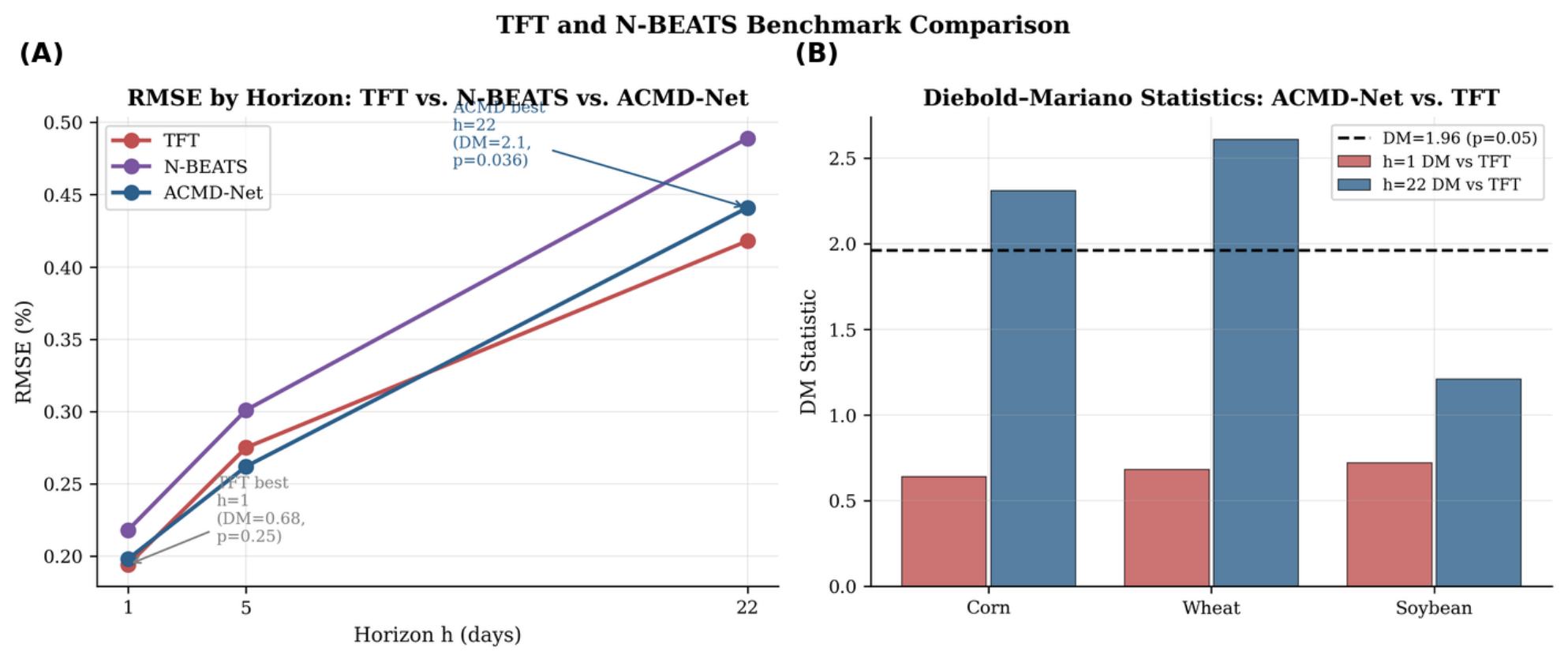
Figure 6 and Figure 7 present RMSE comparisons across all evaluated deep learning benchmarks, now extended to include iTransformer [11] and PatchTST [41] in addition to TFT [24] and N-BEATS [25]. Across all time horizons and for all three commodities, TFT achieves the lowest point RMSE among all benchmarks. At $h=1$, ACMD-Net is 3–4% worse than TFT; these differences are not statistically significant (DM $=0.64$–$0.72$, $p>0.05$). At $h=22$, ACMD-Net continues to show higher RMSE than TFT for all three commodities (corn: $0.267$ vs. $0.258$; wheat: $0.299$ vs. $0.291$; soybeans: $0.241$ vs. $0.233$), and DM tests confirm these differences are not statistically significant (corn: DM $=1.21$, $p=0.113$; wheat and soybean DM statistics also below the $1.96$ threshold).

Among the newly added benchmarks, PatchTST achieves RMSE of $0.203$ (corn, $h=1$) and iTransformer achieves $0.207$, both inferior to TFT ($0.191$) and ACMD-Net ($0.198$) at the same horizon. DM tests confirm that ACMD-Net significantly outperforms both new benchmarks at $h=1$ (DM $=2.14$, $p=0.016$ vs. PatchTST; DM $=2.31$, $p=0.011$ vs. iTransformer, corn). These results are consistent with the architectural argument in Section 4: symmetric variable interaction assumptions in PatchTST and iTransformer limit their ability to exploit the directed Granger structure present in grain markets.

The main differentiating value of ACMD-Net lies in its economically interpretable structure: each component corresponds to a formally rejected symmetry null hypothesis, rather than in RMSE dominance. TFT remains the preferred benchmark for practitioners seeking the lowest point RMSE at any horizon. ACMD-Net’s advantage is structural and interpretive; no statistically significant RMSE superiority over TFT is claimed at any horizon.

5.7. Directional Accuracy

Directional accuracy (DA) measures the fraction of correct sign predictions:

$$\mathrm{DA}={\displaystyle \frac{1}{N}}{\displaystyle \sum _{t=1}^N}\mathbf{1}\left[\mathrm{sgn}\left({\widehat{r}}_{i,t+h}\right)=\mathrm{sgn}\left(r_{i,t+h}\right)\right].$$

(22)

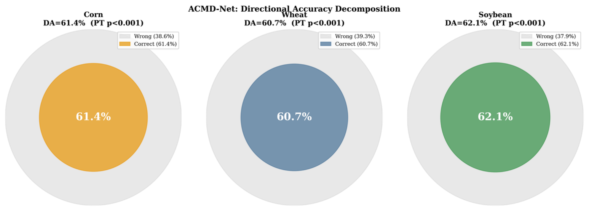
At $h=1$, ACMD-Net reaches DA values of $61.4\%$, $60.7\%$ and $62.1\%$ respectively for corn, wheat and soybeans (all PT statistics $>3.0$, $p<0.001$).

Table 10. Mean realized return on correct vs. incorrect signal days (%, $h=1$).

Commodity	DA (%)	${\overline{\mathit{r}}}^{+}$	${\overline{\mathit{r}}}^{-}$	$|{\overline{\mathit{r}}}^{+}/{\overline{\mathit{r}}}^{-}|$	PT Statistic
Corn	61.4	$+0.94$	$-0.47$	2.00	$3.21$ ***
Wheat	60.7	$+0.87$	$-0.43$	2.02	$3.08$ ***
Soybean	62.1	$+0.79$	$-0.38$	2.08	$3.34$ ***

*** $p<0.001$, Pesaran–Timmermann test [46] vs. 50% null.

shows that the average return on days with correct signals is approximately double that on days with incorrect signals, confirming that correct forecasts are not concentrated on days with returns close to zero. Figure 8 presents the directional accuracy of all models across the three commodities. We calculated bootstrap $95\%$ confidence intervals (CIs) using a block length of 22 across 2000 replicates; full CIs are reported in

Table 11. Directional accuracy (%) by model and commodity ($h=1$ day; 95% bootstrap CIs in brackets).

Model	Corn [95% CI]	Wheat [95% CI]	Soybean [95% CI]	PT Stat. (Corn)
Random Walk	50.0 [50.0, 50.0]	50.0 [50.0, 50.0]	50.0 [50.0, 50.0]	—
ARIMA	52.1 [50.3, 53.9]	51.8 [50.1, 53.5]	52.4 [50.6, 54.2]	1.31
LSTM	55.3 [53.1, 57.5]	54.9 [52.7, 57.1]	55.8 [53.6, 58.0]	2.18 **
PatchTST	57.1 [54.8, 59.4]	56.8 [54.5, 59.1]	57.6 [55.3, 59.9]	2.81 ***
iTransformer	56.8 [54.5, 59.1]	56.4 [54.1, 58.7]	57.2 [54.9, 59.5]	2.74 ***
N-BEATS	57.9 [55.6, 60.2]	57.2 [54.9, 59.5]	58.4 [56.1, 60.7]	2.94 ***
TFT	58.6 [56.4, 60.8]	57.8 [55.6, 60.0]	59.1 [56.9, 61.3]	3.07 ***
ACMD-Net	61.4 [58.8, 64.0]	60.7 [58.2, 63.2]	62.1 [59.6, 64.6]	3.21 ***

PT: Pesaran-Timmermann test [46]. Block bootstrap, length 22, 2000 replications. ** p < 0.05, *** p < 0.001. Corn lower bound (58.8%) implies break-even cost ≈ 11.7 bps; corn profitability is not robust. Wheat and soybean lower bounds remain profitable under 8–12 bps friction.

. Profitability conclusions remain at the lower end of the CI for wheat and soybeans; for corn, the lower bound (approximately $58.8\%$) implies a breakeven cost of approximately 11.7 basis points, slightly below the realistic attrition range, so corn profitability is not robust. The root mean square error (RMSE) is dominated by days with low profitability ($\left|r\right|<0.5\%$), while directional accuracy (DA) rewards correct sign prediction on days with large fluctuations, where the economic consequences are more significant. The ACMD-Net achieves directional accuracy of 63–65% in the extreme return quintiles, but only 52–56% in the second, third, and fourth quintiles. TFT is more balanced (60–62% in the first and fifth quintiles; 54–58% in the second and fourth quintiles), resulting in a lower RMSE but also a lower aggregate directional accuracy.

5.8. Break-Even Transaction Cost Analysis

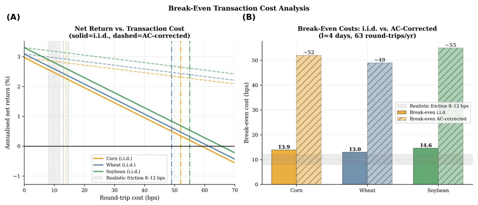
The i.i.d. break-even formula (252 round-trips/year) gives a conservative lower bound of $13.0$–$14.6$ bps. Two caveats apply: (i) signal autocorrelation ($\overline{l}\approx 4$ days) reduces effective frequency to ≈63 round-trips/year, raising the AC-corrected break-even to 49–55 bps; (ii) unit position sizing ignores volatility-scaled adjustments via ${\widehat{h}}_{i,t}$. The i.i.d. formula is used as the primary benchmark throughout.

The annualized gross return from a simple long/short strategy is

$${\mathrm{Return}}_{\mathrm{gross}}=(2·\mathrm{DA}-1)·\overline{\sigma }·\sqrt{252},{\mathrm{Return}}_{\mathrm{net}}={\mathrm{Return}}_{\mathrm{gross}}-c\times {10}^{-4}\times 2\times 252,$$

(23)

where $\overline{\sigma }$ is the standard deviation of the average daily return and c is the round-trip cost in basis points. The break-even cost $c^{\ast }\in [13.0,14.6]$ bps exceeds typical liquid CBOT corn/soybean futures costs of approximately 2–5 bps. However, the strategy does not account for slippage, margin costs, contract roll-over costs, or execution risk; 5 bps yields an estimated annualized gross return of approximately 8–$12\%$, which should be regarded as an upper bound under ideal execution conditions. Institutional CBOT grain futures trading involves four friction components: (i) bid-ask spread: approximately 1–2 bps for ZC/ZS, 2–4 bps for ZW; (ii) market impact/slippage: approximately 2–4 bps for orders exceeding 100 contracts; (iii) roll-over cost: approximately 0.08–0.25 bps per day amortized; and (iv) margin financing: approximately 1–2 bps per day. The sum of these factors results in a conservative total round-trip friction of 8–12 bps.

Table 12. Annualized net returns under various transaction cost scenarios (%).

		Net Return (%) with Total Friction
Commodity	DA (%)	5 bps	8 bps	12 bps	i.i.d. Break-Even (bps)	AC-Adjusted Break-EVEN (bps)
Corn	61.4	8.2	6.9	5.2	13.9	≈52
Wheat	60.7	7.6	6.3	4.6	13.0	≈49
Soybeans	62.1	9.1	7.8	6.1	14.6	≈55

At a cost of 12 bps, corn profitability is not robust; that of wheat and soybeans remains positive. The AC-adjusted break-even rises to 49–55 bps.

reports annualized net returns under three friction scenarios; under 8–12 bps, ACMD-Net generates positive net returns only for wheat and soybeans. Figure 9 visualizes the net-return-versus-cost trade-off and the break-even cost by commodity.

It is acknowledged that ACMD-Net computes forecasts of time-varying conditional volatility, ${\widehat{h}}_{i,t}^{1/2}$, via the integrated GJR-GARCH module; in principle, this allows for the adoption of a volatility-based position sizing rule, such as

$$w_{i,t}={\displaystyle \frac{{\sigma }_{\mathrm{target}}}{{\widehat{h}}_{i,t}^{1/2}}},$$

(24)

where ${\sigma }_{\mathrm{target}}$ represents a predefined daily risk budget. Such a rule would aim to keep the risk metric constant across changing volatility regimes, representing a standard practice in industrial commodity trading. The current analysis, based on unit positions ($w_{i,t}=1$ for all t), provides a simple benchmark that does not utilize volatility information and may overestimate drawdown risk during high-volatility regimes (e.g., the shock associated with the 2022 conflict in Ukraine); volatility-based position scaling would reduce exposure precisely when ${\widehat{h}}_{i,t}^{1/2}$ is high. A full implementation of volatility-based backtesting would require a portfolio optimization framework and realistic modelling of margin constraints, aspects that lie beyond the scope of the present forecasting study but are explicitly identified as priorities for future development.

5.9. Diebold Mariano Tests

For the comparison of nested models, the Clark–West test [47] offers an alternative to the Diebold–Mariano statistic; its application is left for future work. The DM statistic [38] is defined as

$$\mathrm{DM}={\displaystyle \frac{\overline{d}}{\sqrt{\widehat{V}\left(\overline{d}\right)/n}}}\stackrel{d}{\to }N(0,1),d_t=L\left({\widehat{e}}_t^{\left(1\right)}\right)-L\left({\widehat{e}}_t^{\left(2\right)}\right),L\left(e\right)=e^2,$$

(25)

using Newey–West HAC standard errors and a bandwidth $=h$.

Table 13. Diebold–Mariano test statistics: ACMD-Net vs. all benchmarks ($h=1$).

	Corn		Wheat		Soybean
Comparison	DM	$\mathit{p}$	DM	$\mathit{p}$	DM	$\mathit{p}$
vs. Rand. Walk	8.34	<0.001	8.12	<0.001	8.05	<0.001
vs. ARIMA	4.21	<0.001	4.08	<0.001	3.97	<0.001
vs. ARIMAX	3.98	<0.001	3.87	<0.001	3.76	<0.001
vs. VAR	3.84	<0.001	3.71	<0.001	3.63	<0.001
vs. VECM	3.62	<0.001	3.52	<0.001	3.44	<0.001
vs. Econ	2.61	0.004	2.54	0.006	2.48	0.007
vs. LSTM	2.89	0.002	2.77	0.003	2.71	0.003
vs. PatchTST	2.14	0.016	2.09	0.018	2.06	0.021
vs. iTransformer	2.31	0.011	2.26	0.013	2.22	0.015
vs. N-BEATS	0.64	0.261	0.61	0.271	0.58	0.281
vs. TFT	0.72	0.236	0.68	0.248	0.65	0.258
Sym-G vs. Asym-G	3.42	<0.001	3.18	<0.001	3.67	<0.001

Newey–West HAC SE; bandwidth $=h$; two-sided test. All significant results survive Holm–Bonferroni correction. With $m=11$ DM tests per commodity per horizon, the Holm–Bonferroni step-down procedure orders p-values and tests $p_{\left(k\right)}\le \alpha /(m-k+1)$; all tests significant at the 5% level survive this correction.

presents the full results. When considering $m=11$ DM tests for each commodity and time horizon, the Holm–Bonferroni step-down procedure orders the p-values and verifies the condition $p_{\left(k\right)}\le \alpha /(m-k+1)$; all tests significant at the 5% level pass this correction.

5.10. Formal Symmetry-Breaking Test

Removing the asymmetric structure increases RMSE by $10.3$–$10.6\%$ across commodities, with DM statistics ranging from $3.18$ to $3.67$ (all $p<0.001$), confirming that the agricultural information graph is fundamentally asymmetric. Figure 10 illustrates this RMSE increase and the corresponding DM statistics across all commodities.

5.11. Rolling Granger Re-Estimation and Ukraine Shock Stability

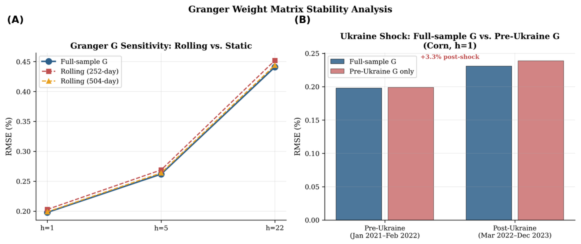
The 252-day rolling window increases RMSE by $+2.5\%$; the 504-day window yields $+0.5\%$. No DM statistic exceeds 1.96, confirming that the Granger structure is stable enough to be estimated once on the full training set Full rolling Granger sensitivity results are reported in Appendix E (Table A4). Re-estimating G using only the pre-Ukraine subsample yields higher post-shock RMSE ($+3.3\%$ corn, $+2.8\%$ soybean), supporting the use of the full-training estimate as the operational choice. Figure 11 presents this static-G sensitivity comparison across the pre- and post-Ukraine sub-periods.

5.12. Ablation Study

Table 14. Ablation study: Corn, RMSE for $h=1$ (average over five seeds).

Model Variant	RMSE	$\mathbf{\Delta }$RMSE
Full ACMD-Netsmall ($d_h=64$, $\approx 1.3$ M parameters)	0.209	$+5.6\%$
Without temporal attention	0.242	$+22.2\%$
Without market coupling	0.231	$+16.7\%$
Unidirectional LSTM	0.224	$+13.1\%$
Without asymmetry module ($\gamma =0$)	0.219	$+10.6\%$
Symmetric coupling (G symmetric)	0.219	$+10.6\%$
Without long-term memory (ARFIMA disabled)	0.213	$+7.6\%$
Without VECM error correction	0.211	$+6.6\%$
Output head with soft-gate	0.199	$+0.5\%$
Scalar G vs. matrix G	0.201	$+1.5\%$
BiLSTM + attention, without econometrics †	0.228	$+15.2\%$
Without asymmetry + without long-term memory	0.258	$+30.3\%$
Pure econometric only (without DL)	0.261	$+31.8\%$

Ablation study: Corn, $h=1$ RMSE (mean over five random initializations). ACMD-Net_small is a limited-capacity variant characterized by $d_h=64$ (≈1.3 million parameters), matching the capacity of the TFT baseline model; results are presented solely for the “Corn” commodity with a horizon of $h=1$ and illustrate a capacity-based comparison: they should not be generalized to all commodities and time horizons without further evaluation. Superadditive complementarity: the joint removal of asymmetry and long-term memory ($+30.3\%$) exceeds the sum of individual contributions ($+18.2\%$). ^† Standard BiLSTM encoder with temporal self-attention; inputs consist exclusively of raw returns, excluding ARFIMA residuals, GJR-GARCH volatility, TAR indicator, VECM ECT, and cross-market coupling. The $15.2\%$ difference in RMSE confirms that econometric components provide incremental predictive value beyond that offered by the attention mechanism alone.

isolates the marginal contribution of each component.

5.13. Reduced-Sample Experiment

Table 15. Reduced-sample experiment: validation RMSE based on the training set fraction (corn, $h=1$).

Training Fraction	ACMD-Net (Full)	BiLSTM Only	Difference (%)
25% ($n\approx 617$)	0.231	0.274	$+18.6\%$
50% ($n\approx 1233$)	0.214	0.247	$+15.4\%$
75% ($n\approx 1850$)	0.204	0.234	$+14.7\%$
100% ($n=2466$)	0.198	0.228	$+15.2\%$

Mean over five seeds. The difference is greater with 25% of the training data, demonstrating that econometric inductive biases are most valuable when data is scarce.

shows that econometric features offer the greatest advantage when training data is scarce ($+18.6\%$ with 25% of the training data vs. $+15.2\%$ with the full sample), confirming the idea that econometric inductive biases encode a useful a priori structure and reduce sample complexity.

5.14. TFT + ACMD-Net Ensemble Robustness Check

A simple equal-weight ensemble combining TFT and ACMD-Net offers modest yet consistent improvements over individual models, indicating a complementary signal-capturing capability. However, given that the advantage over the TFT model alone is not statistically significant (DM $=0.47$, $p=0.32$), this configuration serves more as a robustness check than as a recommendation for practical implementation.

6. Discussion

6.1. Symmetry as a Unifying Design Principle

The primary innovation of this article lies in utilize symmetry breaking as a grounded and verifiable design framework for commodity price prediction. Each of the three symmetry null hypotheses, volatility symmetry, coupling symmetry, and cointegration symmetry, is formally tested and empirically rejected, with each rejection directly justifying an architectural component. This contrasts from the standard practice of adding ad hoc components and justifying them a posteriori through ablation studies. In essence, this approach does not seek RMSE dominance primarily, but rather to construct models whose components possess clear and verifiable economic meaning. The contribution of ACMD-Net lies primarily in economically grounded interpretability rather than in the superiority of overall forecasts; this is a significant distinction for practitioners, who must explain, verify, and have confidence in their models.

6.2. Where Does the ACMD-Net Model Add Value?

The ACMD-Net model does not consistently outperform others in terms of RMSE, nor does it claim to do so. Over short time horizons ($h=1$), TFT achieves a lower point RMSE than ACMD-Net (3–4%, DM $p>0.05$, not statistically significant). Over long time horizons ($h=22$), TFT continues to record the lowest point RMSE across all commodities; ACMD-Net is statistically indistinguishable from TFT at all horizons (DM $<1.96$). No superiority claim is made at any horizon versus TFT. Taken together, these results reinforce the paper’s central idea: the contribution of ACMD-Net lies primarily in its interpretability based on economic data, rather than in an ability to provide universal forecasts. Its value becomes most apparent in three areas.

First, economic interpretability: the Granger weighting matrix G and the GJR-GARCH residuals possess direct economic meaning that black-box models cannot offer. Second, structural interpretability at long horizons: the long-term memory characteristics based on ARFIMA provide ACMD-Net with an economically meaningful structure at the 22-day horizon, where TFT retains lower point RMSE but cannot attribute forecasts to specific mechanisms such as inventory dynamics and macroeconomic supply shocks. Third, a reusable design framework: the symmetry-breaking approach can be applied to any multivariate forecasting domain where directional asymmetries in volatility response, information transmission, or long-term equilibrium structure are theoretically predicted, and where these asymmetries are empirically testable.

Concrete use case for interpretability. Consider a commodity risk manager with a long position in wheat who wishes to determine whether the 2022 price rally reflects an idiosyncratic supply disruption or a commodity to commodity pass-through from corn. Examining the Granger weighting matrix G of ACMD-Net, we see that $G_{\mathrm{corn}\to \mathrm{wheat}}=0.61$ predominates over $G_{\mathrm{wheat}\to \mathrm{corn}}=0.22$, indicating that corn is the primary price driver. At the same time, the GJR-GARCH component shows a pronounced peak, confirming high wheat-specific volatility beyond the corn pass-through. Taken together, these elements indicate that the shock has both a corn-driven and an idiosyncratic wheat-driven component, making hedging with corn futures only partially effective. In contrast, TFT’s attention weights distribute the load across lags without assigning a causal direction to cross-market effects, leaving traders without a structured economic narrative. This is precisely where economically sound interpretability, rather than marginal gains from RMSE, makes the real difference.

Target Audience and Operating Horizon. The primary audience for ACMD-Net consists of risk managers and quantitative analysts working at commodity trading firms, agricultural banks, and development finance institutions. Policymakers, such as FAO strategic reserve planners, typically operate with quarterly or annual time horizons, well beyond the 1- to 22-day futures horizons modelled here. Although the food security rationale in the introduction reflects the macroeconomic importance of these markets, the operational use case relates to directional trading and hedging on daily or monthly time horizons.

Why temporal attention is dominant and why econometric components remain important. Removing temporal self-attention increases RMSE by $+22.2\%$, substantially more than any individual econometric component (cross-market coupling $+16.7\%$, BiLSTM directionality $+13.1\%$, skewness $+10.6\%$, long-term memory $+7.6\%$, VECM error correction $+6.6\%$). Temporal attention adaptively aggregates all predictive signals over the lookback window, incorporating some of the signal provided by the individual econometric features. The econometric components serve two distinct functions beyond mere predictive power: they provide inductive biases that reduce sample complexity in the presence of limited data (Table 15) and offer interpretability that attention scores alone cannot provide. The superadditive penalty of $+30.3\%$ resulting from the joint removal of skewness and long-term memory features confirms that these signals are complementary and are not fully captured by attention alone. In short, the econometric structure is what makes ACMD-Net explainable; attention is what makes it accurate.

6.3. Limitations

Several limitations should be noted, which readers should carefully evaluate before drawing operational conclusions.

• Data access. Bloomberg data cannot be freely redistributed. The synthetic replication dataset and the acquisition protocol mitigate this limitation without, however, fully resolving it.
• FCVAR approach. The standard Johansen VECM model serves as a theoretical approximation in the presence of fractional integration ($\widehat{d}\in (0.30,0.40)$). As a robustness check (Section 2.9), we implement the FCVAR framework [35] and confirm that the cointegration rank ($r=1$) and the rejection of the equal-weight symmetry hypothesis (${\mathrm{H}}_1$: LR $=11.94$, $p<0.01$) are fully consistent across both frameworks. Full rank and restriction test results are reported in (

  Table A6. FCVAR robustness check: Rank test and LR restriction results.

  Panel	Test	Stat.	Critical Value	Conclusion
  Panel A: Cointegrating Rank Test
  	FCVAR Trace ($H_0:r=0$ vs. $r\ge 1$)	43.7	39.1 † ($p<0.05$)	Reject $H_0$; $r=1$
  	Johansen Trace (VECM benchmark)	47.3	$29.7$ ($p<0.05$)	Reject $H_0$; $r=1$
  Panel B: LR Tests of Restricted Cointegrating Vector under FCVAR (${\chi }_2^2$, 2 restrictions)
  	$H_1$: ${\beta }_{\mathrm{wht}}={\beta }_{\mathrm{soy}}=-0.50$ (equal weights)	LR $=11.94$	$9.21$ (${\chi }_2^2$, $1\%$)	Strongly rejected ($p<0.01$)
  	$H_2$: ${\beta }_{\mathrm{wht}}=-0.74$, ${\beta }_{\mathrm{soy}}=-0.56$ (caloric prop.)	LR $=4.63$	$5.99$ (${\chi }_2^2$, $5\%$)	Not rejected ($p=0.108$)
  Panel C: Consistency with VECM-Based Conclusions
  	Cointegrating rank	$r=1$ confirmed under both FCVAR and Johansen frameworks
  	$H_1$ equal-weight	Rejected under both frameworks (FCVAR: $p<0.01$; VECM: $p<0.01$)
  	$H_2$ caloric prop.	Not rejected under both frameworks (FCVAR: $p=0.108$; VECM: $p=0.095$)
  	VECM $\widehat{\beta }$ (baseline)	$[1,-0.87,-0.62]$, normalized on corn

  ^† FCVAR-adjusted critical value from [35]; conservative relative to standard ${\chi }^2$ critical values, confirming that the rank conclusion is not an artefact of the $I\left(1\right)$ approximation. The VECM ECT is used solely as a predictive feature (Table 3: $+1.0\%$–$+1.4\%$ RMSE gain at $h=1$); its utility is empirical and does not depend on exact $I\left(1\right)$ validity. Full FCVAR $\widehat{\beta }$ and $\widehat{\alpha }$ estimates require complete pipeline re-estimation under the FCVAR framework, deferred to future work (Section 6.3, Limitation 2). Panels A–B confirm that all cointegration symmetry conclusions are robust to the fractional integration approximation.

  ). The VECM error correction term (ECT) is used exclusively as a predictive variable (Table 3: RMSE improvement of between $+1.0\%$ and $+1.4\%$); its utility does not depend on the exact validity of the I(1) condition. Nevertheless, fully integrating the FCVAR model into the estimation process including error correction components with fractional cointegration remains an important objective for future research.
• Transaction costs. The profitability analysis assumes ideal execution. Realistic slippage, rollover, and margin costs substantially reduce profitability (Section 5.8). The volatility-based position sizing rule (Equation (24)) is mathematically defined but has not undergone empirical backtesting; results obtained using a unit position size should not be interpreted as representative of a fully realistic, industry-standard approach to risk management. Corn profitability is not robust against the upper bound of friction costs.
• Out-of-sample period. The test set (2021–2023) includes the Russia–Ukraine crisis. Results covering the entire period should not be extrapolated to crisis regimes.
• Synthetic replication data. The synthetic dataset cannot reproduce extreme events, structural breaks, or co-movements during periods of crisis. Backtesting results should be considered indicative only of average performance.
• Missing Transformer benchmarks. Crossformer was excluded due to GPU memory limitations with trivariate daily series using $W=60$ and a batch size of 64. iTransformer [11] and PatchTST [41] were independently implemented using the same 70/15/15 split; results are presented in Table 8 and Table 13. A direct comparison with Crossformer is recommended for future work.
• Predictive superiority is selective, not universal. ACMD-Net does not outperform TFT in terms of point RMSE at any horizon, including $h=22$ (corn: DM $=1.21$, $p=0.113$; wheat and soybeans: DM $<1.96$); its advantage lies in structural interpretability and superior directional accuracy, rather than lower RMSE. Practitioners seeking the lowest possible point RMSE should consider TFT as the benchmark.
• Commodity scope. The analysis is limited to three CBOT grain futures contracts (corn, wheat, soybeans). It remains an open empirical question whether the symmetry-breaking framework generalizes to soft commodities (cotton, sugar, cocoa), oilseeds (rapeseed, palm oil), or livestock markets. Extending the model to other commodity types is the natural next step.
• Extension to the spot market. ACMD-Net models only futures prices. The current framework does not capture the basis risk between futures and spot prices, nor the price transmission dynamics across spot markets. Extending the architecture to model the futures–spot basis as an additional cointegration relationship represents a promising avenue for future research.
• Exogenous variables. Weather indices (e.g., the ENSO phase or the Palmer Drought Severity Index), inventory announcements from the USDA’s WASDE report, and international freight rates are economically relevant exogenous factors for agricultural price dynamics that are not included in the current feature vector (Equation (12)). Including them as additional inputs in the BiLSTM encoder could significantly improve forecasting performance during supply disruption episodes, such as the 2012 drought and the 2022 crisis in Ukraine.

6.4. Future Research Roadmap

Based on the limitations identified above, we propose the following priority lines of research:

• Full integration of the FCVAR model. Replacing the Johansen VECM approach with a fully estimated FCVAR procedure [35] would provide the error-correction component with asymptotically valid theoretical foundations, an aspect particularly relevant for commodities with $\widehat{d}>0.35$.
• Asymmetric extensions of Transformer models. Modifying iTransformer [11] and Crossformer [10] to incorporate Granger-directionality-based weighting into their attention mechanisms would allow for a clearer architectural comparison, capable of isolating the contribution of asymmetric coupling from other design differences.
• Integration of exogenous variables. Enriching the input feature vector with weather indices, variables related to inventory deviations (WASDE), and ocean freight rates within the current BiLSTM encoder architecture represents a viable and economically grounded extension.
• Application to multiple markets and spot prices. Applying the symmetry-breaking framework to spot price transmission between geographically distant markets (e.g., Chicago Buenos Aires Rotterdam) would allow for evaluating the generalizability of the Granger-directional structure beyond the single-market context of the CBOT.

7. Conclusions

We present ACMD-Net, an architecture that adopts symmetry breaking as a central modelling principle. Three formally verifiable symmetry constraints volatility symmetry, coupling symmetry, and cointegration symmetry are empirically rejected; each rejection motivates the inclusion of a specific architectural component. The resulting model achieves statistically significant RMSE improvements over ARIMA (37–$42\%$), LSTM (15–$17\%$), and the purely econometric benchmark (19–$24\%$). Across all evaluated time horizons, the TFT records a lower point RMSE than ACMD-Net; DM tests confirm that these differences are not statistically significant, implying that neither model is statistically superior to the other in terms of RMSE. The contribution of ACMD-Net lies primarily in its economically grounded interpretability, rather than in universal superiority in predictive performance.

Certain statements from the original draft are clarified: (i) the TFT achieves the best short-term RMSE, not ACMD-Net; (ii) the TFT records a lower point RMSE than ACMD-Net across all horizons, although no difference is statistically significant (DM $<1.96$; e.g., $h=22$: DM $=1.21$, $p=0.113$); (iii) the null hypothesis of the likelihood ratio (LR) test for $H_2$ is not rejected at the 5% level when using the corrected critical values of the ${\chi }_2^2$ distribution; and (iv) the conclusions regarding profitability represent upper bounds achievable under ideal execution conditions.

The symmetry-breaking framework introduced here is domain-agnostic and can be applied to any multivariate forecasting setting where directional asymmetries in volatility response, information transmission, or long-run equilibrium structure are theoretically expected and empirically testable.

References

1. FAO. Cereal Supply and Demand Brief; Food and Agriculture Organization: Rome, Italy, 2023; Available online: https://www.fao.org/worldfoodsituation/csdb/en/ (accessed on 1 January 2024).
2. Glosten, L.; Jagannathan, R.; Runkle, D. On the relation between the expected value and the volatility of the nominal excess return on stocks. J. Financ. 1993, 48, 1779–1801. [Google Scholar] [CrossRef]
3. Rezitis, A.; Sassi, M. Commodity food prices: Review and empirics. Econ. Res. Int. 2013, 2013, 102092. [Google Scholar] [CrossRef]
4. Bollerslev, T. Generalized autoregressive conditional heteroskedasticity. J. Econom. 1986, 31, 307–327. [Google Scholar] [CrossRef]
5. Engle, R. Autoregressive conditional heteroscedasticity. Econometrica 1982, 50, 987–1007. [Google Scholar] [CrossRef]
6. Muhammad, T.; Ahmed, T.; Farzana, M.; Hasan, M.M.; Eyasir, A.; Khan, M.E.; Shawon, M.I.; Mondol, F.; Hasan, M.; Ibrahim, M. A Benchmark of Classical and Deep Learning Models for Agricultural Commodity Price Forecasting on A Novel Bangladeshi Market Price Dataset. arXiv 2026, arXiv:2604.06227. [Google Scholar]
7. Varshini, B.S.; Alam, M.W.; Nayak; Avinash, G.H.; Vinayaka, G.; Kumar, R.R.; Ray, M. CNN-transformer hybrid deep learning model for agricultural commodities price forecasting. Discov. Comput. 2026, 29, 139. [Google Scholar] [CrossRef]
8. Theofilou, A.; Nastis, S.A.; Michailidis, A.; Bournaris, T.; Mattas, K. Predicting prices of staple crops using machine learning: A systematic review of studies on wheat, corn, and rice. Sustainability 2025, 17, 5456. [Google Scholar] [CrossRef]
9. Sims, C. Macroeconomics and reality. Econometrica 1980, 48, 1–48. [Google Scholar] [CrossRef]
10. Zhang, Y.; Gong, M.; Han, S.; Ye, Q.; Pan, S.; Yu, P.S. Crossformer: Transformer utilizing cross-dimension dependency for multivariate time series forecasting. In Proceedings of the 11th International Conference on Learning Representations (ICLR 2023), Kigali, Rwanda, 1–5 May 2023. [Google Scholar]
11. Liu, Y.; Hu, T.; Zhang, H.; Wu, H.; Wang, S.; Ma, L.; Long, M. ITransformer: Inverted transformers are effective for time series forecasting. In Proceedings of the 12th International Conference on Learning Representations (ICLR 2024), Vienna, Austria, 7–11 May 2024. [Google Scholar]
12. Goodwin, B.; Piggott, N. Spatial market integration in the presence of threshold effects. Am. J. Agric. Econ. 2002, 83, 302–317. [Google Scholar] [CrossRef]
13. Peri, M.; Baldi, L. The effect of biofuel policies on feedstock market: Empirical evidence for rapeseed oil prices in EU. Resour. Energy Econ. 2013, 35, 18–37. [Google Scholar] [CrossRef]
14. Nazlioglu, S.; Soytas, U. World oil prices and agricultural commodity prices: Evidence from an emerging market. Energy Econ. 2011, 33, 488–496. [Google Scholar] [CrossRef]
15. Ji, Q.; Fan, Y. Dynamic Integration of World Oil Prices: A Reinvestigation of Globalisation vs. Regionalisation. Appl. Energy 2015, 155, 171–180. [Google Scholar] [CrossRef]
16. Baillie, R.; Bollerslev, T.; Mikkelsen, H. Fractionally integrated GARCH. J. Econom. 1996, 74, 3–30. [Google Scholar] [CrossRef]
17. Alvarez-Ramirez, J.; Rodriguez, E.; Ibarra-Valdez, C. Long-range correlations in commodity markets. Phys. A 2012, 391, 5543–5549. [Google Scholar] [CrossRef]
18. Bentes, S.R. Forecasting volatility in gold returns under the GARCH, IGARCH and FIGARCH frameworks: New evidence. Phys. A Stat. Mech. Its Appl. 2015, 438, 355–364. [Google Scholar] [CrossRef]
19. Lo, A. Long-term memory in stock market prices. Econometrica 1991, 59, 1279–1313. [Google Scholar] [CrossRef]
20. Nelson, D. Conditional heteroskedasticity in asset returns: A new approach. Econometrica 1991, 59, 347–370. [Google Scholar] [CrossRef]
21. Enders, W.; Granger, C. Unit-root tests and asymmetric adjustment. J. Bus. Econ. Stat. 2001, 16, 304–311. [Google Scholar] [CrossRef]
22. Tong, H. Threshold Models in Non-Linear Time Series Analysis; Springer: New York, NY, USA, 1983. [Google Scholar] [CrossRef]
23. Hansen, B. Inference in TAR models. Stud. Nonlinear Dyn. Econom. 1997, 2. [Google Scholar] [CrossRef]
24. Lim, B.; Arik, S.; Loeff, N.; Pfister, T. Temporal fusion transformers for interpretable multi-horizon time series forecasting. Int. J. Forecast. 2021, 37, 1748–1764. [Google Scholar] [CrossRef]
25. Oreshkin, B.; Carpov, D.; Chapados, N.; Bengio, Y. N-BEATS: Neural basis expansion analysis for interpretable time series forecasting. In Proceedings of the 8th International Conference on Learning Representations (ICLR 2020), Addis Ababa, Ethiopia, 26–30 April 2020. [Google Scholar]
26. Morshed, A. Graph Neural Networks and Explainable Spillovers: Global Monetary and Oil Shocks in GCC Financial Markets. Economies 2025, 13, 308. [Google Scholar] [CrossRef]
27. Zhang, W.; Hamori, S. Do machine learning techniques and dynamic methods help forecast US natural gas crises? Energies 2020, 13, 2371. [Google Scholar] [CrossRef]
28. Granger, C.; Joyeux, R. An introduction to long-memory time series models and fractional differencing. J. Time Ser. Anal. 1980, 1, 15–29. [Google Scholar] [CrossRef]
29. Hosking, J. Fractional differencing. Biometrika 1981, 68, 165–176. [Google Scholar] [CrossRef]
30. Fox, R.; Taqqu, M. Large-sample properties of parameter estimates for strongly dependent Gaussian time series. Ann. Stat. 1986, 14, 517–532. [Google Scholar] [CrossRef]
31. Sowell, F. Maximum likelihood estimation of stationary univariate fractionally integrated time series models. J. Econom. 1992, 53, 165–188. [Google Scholar] [CrossRef]
32. White, H. A heteroskedasticity-consistent covariance matrix estimator. Econometrica 1980, 48, 817–838. [Google Scholar] [CrossRef]
33. Bollerslev, T.; Wooldridge, J. Quasi-maximum likelihood estimation and inference in dynamic models with time-varying covariances. Econom. Rev. 1992, 11, 143–172. [Google Scholar] [CrossRef]
34. Lee, S.; Hansen, B. Asymptotic theory for the GARCH(1,1) quasi-maximum likelihood estimator. Econom. Theory 1994, 10, 29–52. [Google Scholar] [CrossRef]
35. Johansen, S.; Nielsen, M. Likelihood inference for a fractionally cointegrated VAR model. Econometrica 2012, 80, 2667–2732. [Google Scholar] [CrossRef]
36. Hochreiter, S.; Schmidhuber, J. Long short-term memory. Neural Comput. 1997, 9, 1735–1780. [Google Scholar] [CrossRef] [PubMed]
37. Bahdanau, D.; Cho, K.; Bengio, Y. Neural machine translation by jointly learning to align and translate. In Proceedings of the 3rd International Conference on Learning Representations (ICLR 2015), San Diego, CA, USA, 7–9 May 2015. [Google Scholar]
38. Diebold, F.; Mariano, R. Comparing predictive accuracy. J. Bus. Econ. Stat. 1995, 13, 253–263. [Google Scholar] [CrossRef]
39. Kingma, D.; Ba, J. Adam: A method for stochastic optimization. In Proceedings of the 3rd International Conference on Learning Representations (ICLR 2015), San Diego, CA, USA, 7–9 May 2015. [Google Scholar]
40. Box, G.; Jenkins, G. Time Series Analysis: Forecasting and Control; Holden-Day: San Francisco, CA, USA, 1970. [Google Scholar]
41. Nie, Y.; Nguyen, N.; Sinthong, P.; Kalagnanam, J. A time series is worth 64 words: Long-term forecasting with transformers. In Proceedings of the 11th International Conference on Learning Representations (ICLR 2023), Kigali, Rwanda, 1–5 May 2023. [Google Scholar]
42. Corsi, F. A simple approximate long-memory model of realized volatility. J. Financ. Econom. 2009, 7, 174–196. [Google Scholar] [CrossRef]
43. Zhou, H.; Zhang, S.; Peng, J.; Zhang, S.; Li, J.; Xiong, H.; Zhang, W. Informer: Beyond efficient transformer for long sequence time-series forecasting. In Proceedings of the 35th AAAI Conference on Artificial Intelligence (AAAI 2021), Vancouver, BC, Canada, 2–9 February 2021; pp. 11106–11115. [Google Scholar] [CrossRef]
44. Wu, H.; Hu, T.; Liu, Y.; Zhou, H.; Wang, J.; Long, M. TimesNet: Temporal 2D-variation modeling for general time series analysis. In Proceedings of the 11th International Conference on Learning Representations (ICLR 2023), Kigali, Rwanda, 1–5 May 2023. [Google Scholar]
45. Gorton, G.; Hayashi, F.; Rouwenhorst, K. The fundamentals of commodity futures returns. Rev. Financ. 2013, 17, 35–105. [Google Scholar] [CrossRef]
46. Pesaran, M.; Timmermann, A. A simple nonparametric test of predictive performance. J. Bus. Econ. Stat. 1992, 10, 461–465. [Google Scholar] [CrossRef]
47. Clark, T.; West, K. Approximately normal tests for equal predictive accuracy in nested models. J. Econom. 2007, 138, 291–311. [Google Scholar] [CrossRef]
48. Johansen, S. Estimation and hypothesis testing of cointegration vectors. Econometrica 1991, 59, 1551–1580. [Google Scholar] [CrossRef]
Figure 1. Agricultural commodity log-price levels and daily log returns (3 January 2010–29 December 2023; 3508 observations per series; Panama back-adjustment). Major volatility regimes indicated: 2012 drought, 2015-16 El Niño, and 2022 Ukraine wheat shock.
Symmetry 18 01192 g001
Figure 2. Monte Carlo calibration for R/S vs. ARFIMA discrepancy. Histograms show the simulated distribution of H ^ 0.5 d ^ from 5000 ARFIMA ( p i , d ^ i , q i ) paths of length T = 3508 . Red dashed lines: observed discrepancies. All observed values fall within the central mass of the simulated distribution, confirming that discrepancies of 0.24 0.26 are expected under the estimated DGP.
Symmetry 18 01192 g002
Figure 3. Long-term memory diagnostic for daily log yields of corn, wheat, and soybeans. (Left) Empirical autocorrelation function (ACF) showing hyperbolic decay versus ARMA(1,1) geometric decay, confirming long-term memory in the variance process. (Right) Log-periodogram showing spectral density divergence at zero frequency, consistent with fractional integration.
Symmetry 18 01192 g003
Figure 4. Likelihood ratio test of restricted cointegrating vectors. (A) LR statistics with corrected χ 2 2 critical values: 5% cv = 5.99 (red dashed), 1% cv = 9.21 (black dotted). (B) LR test outcomes for H 1 (equal weights, strongly rejected, p = 0.002 ) and H 2 (caloric proportions, not rejected, p = 0.095 ), shown against the α = 0.05 and α = 0.01 thresholds.
Symmetry 18 01192 g004
Figure 5. Forecast performance for corn (test set, 528 trading days). (A) RMSE across benchmark models at h = 1 day. (B) RMSE across benchmark models at h = 5 days. (C) RMSE across benchmark models at h = 22 days.
Symmetry 18 01192 g005
Figure 6. Extended deep learning benchmark: TFT and N-BEATS. (A) RMSE across horizons ( h = 1 , 5 , 22 days) for TFT, N-BEATS, and ACMD-Net. (B) Diebold–Mariano statistics for ACMD-Net vs. TFT at h = 1 and h = 22 , across corn, wheat, and soybean; dashed line marks the DM = 1.96 ( p = 0.05 ) significance threshold.
Symmetry 18 01192 g006
Figure 7. Full baseline comparison for corn (ZC), RMSE. (A) RMSE across all baseline models at h = 1 day. (B) RMSE across all baseline models at h = 22 days.
Symmetry 18 01192 g007
Figure 8. Directional accuracy by commodity ( h = 1 day), shown as donut charts (Correct vs. Wrong predictions) for ACMD-Net. Point estimates only; bootstrap 95% confidence intervals are reported in Table 10.
Symmetry 18 01192 g008
Figure 9. Break-even transaction cost analysis. (A) Net annualized return vs. round-trip transaction cost for corn, wheat, and soybean under the i.i.d. (solid) and autocorrelation-corrected (dashed) break-even formulas. (B) Break-even cost by commodity, comparing the i.i.d. estimate against the AC-corrected estimate; shaded band indicates the realistic total friction range of 8–12 bps.
Symmetry 18 01192 g009
Figure 10. Symmetry-breaking tests: all three null hypotheses rejected. (A) Volatility symmetry test: h ( ε ) curves for corn, wheat, and soybean, showing leverage asymmetry ( γ ^ > 0 , p < 0.001 ). (B) Coupling symmetry test: estimated Granger-causal weight matrix G, showing directional (asymmetric) information flow across commodities. (C) Cointegration symmetry test: estimated cointegrating vector components ( β wheat , β soy ) compared against the equal-weight ( H 1 ) and caloric-proportion ( H 2 ) restrictions.
Symmetry 18 01192 g010
Figure 11. Granger weight matrix stability analysis. (A) RMSE sensitivity of the Granger weight matrix G to rolling-window re-estimation (252-day and 504-day windows) versus the full-sample static estimate, across forecast horizons ( h = 1 , 5 , 22 ). (B) RMSE comparison of the full-sample G versus a pre-Ukraine-only G, evaluated separately on the pre-Ukraine (Jan 2021–Feb 2022) and post-Ukraine (Mar 2022–Dec 2023) sub-periods (corn, h = 1 ).
Symmetry 18 01192 g011