Article

Distribution Network Hosting Capacity Assessment Method of Electric Vehicle Charging Stations Based on Multi-Zone Load Profiling
Jiangsu Electric Power Test Research Institute Co., Ltd., Nanjing 211100, China
*
Author to whom correspondence should be addressed.
Symmetry 2026, 18(6), 990; https://doi.org/10.3390/sym18060990
Submission received: 17 May 2026 / Revised: 3 June 2026 / Accepted: 5 June 2026 / Published: 9 June 2026
(This article belongs to the Special Issue Symmetry with Power Systems: Control and Optimization)

Abstract

Fast growth in electric vehicle (EV) charging stations is changing the way regional distribution networks are loaded. The difficulty is not only the size of the added demand, but also the fact that charging appears at different places, at different times, and under different voltage constraints. This paper considers the common planning situation in which station-level charging records are incomplete and only transformer-side aggregate measurements are available. A data-driven hosting capacity (HC) assessment method is developed for this setting. The method first constructs zone-specific daily load profiles and then separates EV charging components from mixed transformer curves through an improved ISODATA clustering method and an improved genetic algorithm (IGA). For planned electric vehicle charging stations (EVCSs) without historical measurements, Ordinary Kriging (OK) is used to infer charging profiles from nearby observed stations in the same functional zone. The calculated HC is then checked successively at the 10 kV, 35 kV, and 110 kV levels. When an upstream constraint is violated, an improved Entropy-weight TOPSIS (EW-TOPSIS) model reallocates the available capacity according to both network constraints and zone priority. The case study indicates that the method can identify upstream bottlenecks that are hidden in local assessments, preserve residential charging demand, and provide zone-specific guidance for EVCS expansion.

1. Introduction

Transport electrification is now a major route for meeting carbon peaking and carbon neutrality targets. For distribution utilities, however, the pressure created by EV adoption is not a simple increase in annual energy consumption. Charging load enters the network with strong temporal and spatial uncertainty, and it is often connected to feeders whose monitoring and regulation capabilities were designed for more regular demand. Recent studies on charging-station infrastructure show that the practical challenge also involves equipment standards, policy coordination, and the connection of charging facilities to existing distribution assets [1]. EV charging demand has been shown to vary sharply across both space and time [2]. Without coordination, it can worsen voltage regulation, increase peak-valley imbalance, and disturb active distribution-network operation [3]. In weakly monitored residential areas, concentrated charging may further accelerate transformer aging, increase losses and harmonics, and raise the probability of equipment failure at edge transformers [4].
Hosting capacity (HC) is therefore a useful planning index, because it translates those operational concerns into the amount of new charging demand that a network can accept. In [5], HC is described as the maximum level of distributed resources, including EV charging demand or photovoltaic generation, that can be accommodated without violating operating limits or requiring major reinforcement. For EVCS planning, this index supports site screening, investment timing, and secure operation. The review in [6] also shows a clear shift in HC studies: early index-based calculations have been supplemented by methods that represent load behavior, evaluate dynamic capacity, and coordinate enhancement measures.
The symmetry issue considered in this paper appears when EVCS integration is compared with the ideal case of complete and evenly distributed information. If charging demand, metering data, and spare capacity were all available at the same resolution, HC could be assessed in a nearly uniform manner across nodes and voltage levels. Actual distribution networks rarely have that property. Residential, commercial, office, and mixed-use zones produce different charging patterns; user-side charging records and transformer-side aggregate curves are collected with different granularity; and the spare margins of 10 kV, 35 kV, and 110 kV assets are uneven. A useful HC method should therefore quantify these asymmetries instead of treating the system as a set of homogeneous loads with identical capacity margins.
The framework proposed in this paper links non-intrusive load decomposition, spatial interpolation, and hierarchical HC calculation under limited data availability. Existing EV load-modeling research can be grouped roughly into statistical simulation and data-driven approaches. In early planning studies, EV charging curves were often produced from probability distributions. For instance, ref. [7] estimated distributions for daily mileage and charging start time from household travel survey data and then generated charging curves through random sampling. Such approaches are convenient for scenario analysis, but [8] notes that they rely heavily on assumed distributions and may not capture the diversity of individual charging behavior.
AMI deployment has made data-driven EV modeling more feasible [9], but the available data are still uneven in many distribution systems. Regression-based models can map historical explanatory variables to charging demand or HC when paired training samples are complete. Their limitation in this study is different: the EV charging component is mixed into the transformer aggregate curve, and the final HC must also respect the constraints of the 10 kV, 35 kV, and 110 kV layers. For that reason, this paper first reconstructs EV charging profiles by combining multi-zone profiling with non-intrusive decomposition, and then verifies HC through a time-series and hierarchical process. The choice is driven by a practical data barrier: marketing-side charging records and distribution-side measurements are often stored separately, while low-voltage transformers are usually observed only through master-meter readings. Under these sparse-measurement conditions, sub-loads cannot be read directly. Similar problems have been reported in unbalanced active distribution networks [10]. Operators therefore need a way to recover EVCS charging curves from mixed-load measurements. Accurate reconstructed curves are also needed for aggregation, market participation, and ramping analysis [11]. Without such curves, HC assessment becomes dependent on idealized sub-metering assumptions rather than on the data actually available to network operators.
Once load composition is known, the assessment method itself becomes the next concern. Current HC studies usually rely on static, dynamic time-series, or probabilistic assessment. Static methods examine the network under a limited number of severe operating points, such as the evening peak. For example, ref. [12] increases EV penetration step by step until a constraint is reached. This procedure is easy to implement, but it can miss the temporal complementarity between background load and EV charging, which may lead to conservative capacity estimates [13]. Dynamic and probabilistic methods reduce this weakness by representing uncertainty and time variation. Reference [14] uses a cumulant-based probabilistic model to account for uncertainty in demand and renewable generation; [15] introduces an interval undervoltage probability index; and [16] formulates a chargeable-region optimization model for EV accommodation. These studies improve accuracy, but they do not by themselves solve the question of whether capacity accepted at the low-voltage level remains feasible after aggregation to superior voltage levels.
A second limitation is that many HC methods still focus on one voltage layer. Although [17] includes both medium- and low-voltage networks, a large part of the literature evaluates the distribution system as though it were separated from the upstream grid. Recent data-driven work has improved voltage-security assessment in active distribution networks, but its focus is usually the security boundary itself rather than bottom-up HC consistency across voltage levels [18]. When EV penetration increases, the interaction between transmission and distribution cannot be ignored [19]. A feeder may satisfy its own local constraints while the summed charging demand still overloads an upstream substation. This is the reason hierarchical verification is treated here as part of the HC calculation rather than as a later screening step.
When the calculated HC is insufficient, capacity enhancement or demand adjustment is required. Reinforcing lines and transformers is reliable, but it is costly and slow to deploy. Many studies therefore examine soft-control measures, including smart charging, demand-side management, vehicle-to-grid operation, and coordinated charging dispatch [20]. Time-of-use pricing and direct charging control can reduce peak demand and increase effective HC [21,22]. Other studies use local voltage measurements [23], operational HC indicators for low-voltage networks [24], or distributed demand-response controllers [25]. These methods help relieve congestion, but the curtailment rule is often driven mainly by technical sensitivity or proportional reduction. In real EVCS planning, the service role of a zone also matters: basic residential charging demand may need stronger protection than more flexible commercial charging demand.
From the symmetry/asymmetry viewpoint used in this paper, three gaps remain. First, many data-driven models, including [26,27], assume balanced observability or complete sub-metering, while actual distribution networks often contain only transformer-level aggregate measurements and incomplete user-side charging records. EV load extraction is then a mixed-load separation problem rather than a direct prediction task. Second, spatial heterogeneity in charging demand has been discussed in urban parking and charging studies [28], but those models do not usually include distribution-network capacity limits. Third, several HC studies, such as [29], treat stations or voltage layers as broadly comparable units, which hides the differences among functional zones and the unequal spare margins of 10 kV, 35 kV, and 110 kV equipment. Existing reallocation methods [30,31] also tend to be uniform or purely technical, with limited attention to priority among zones. These gaps motivate an assessment framework that links load profiling, hierarchical verification, and differentiated capacity adjustment.
This paper therefore proposes a data-driven HC assessment framework in which asymmetric load behavior, asymmetric measurement availability, and asymmetric capacity margins are handled together. The contributions are threefold. (1) A non-intrusive load-decomposition method is designed for cases where EV charging is embedded in aggregate transformer measurements. Improved ISODATA clustering and IGA are combined to separate EV charging signals without requiring complete sub-metering. (2) A multi-zone profiling and spatial interpolation procedure is used to estimate charging curves for planned EVCSs. OK interpolation transfers profile weights from observed stations to unobserved sites within the same functional zone. (3) A hierarchical HC verification and reallocation mechanism is built for 10 kV, 35 kV, and 110 kV networks. The improved EW-TOPSIS model then distributes the required adjustment according to technical constraints and functional-zone priority. A comparison between the proposed framework and representative EV HC assessment methods is summarized in Table 1.

2. Materials and Methods

2.1. Framework Overview

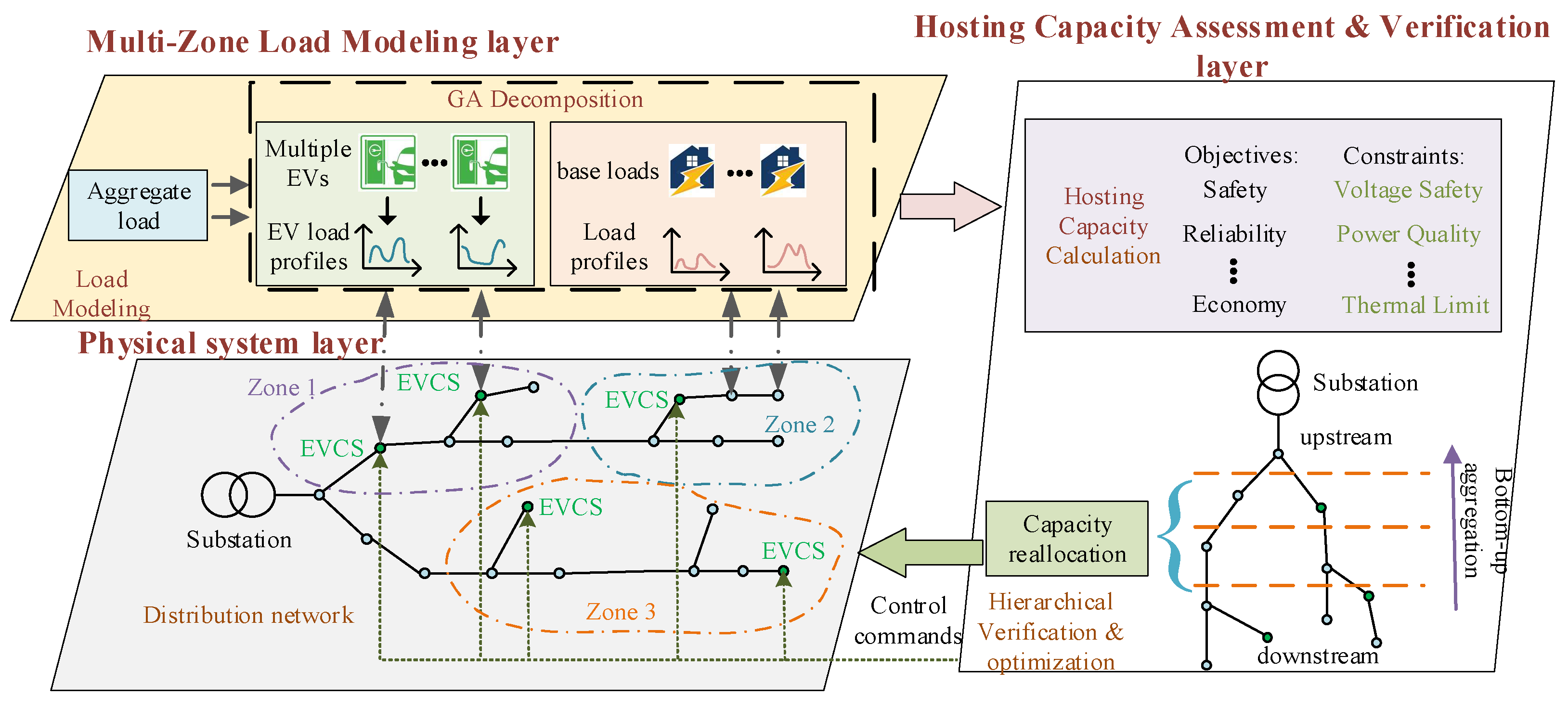
A data-driven HC assessment framework for EVCSs is constructed around multi-zone load profiling. The framework is intended for three data and planning difficulties that frequently appear together: the load components at existing transformer nodes are mixed, planned stations have no local history, and local capacity decisions may be invalid after the demand is aggregated to higher voltage levels. Figure 1 organizes the method into four stages:
The first stage classifies distribution nodes into residential, commercial, and public-service zones according to land-use characteristics. Historical aggregate load curves are processed by the improved ISODATA method to obtain representative base-load and EV-load profiles for each zone. These profiles form the library used in the later decomposition. For transformer nodes with historical measurements, the IGA-based decomposition model expresses the measured nodal curve as a weighted combination of typical base-load and EV-load profiles, so that the EV component can be extracted from the mixed measurement. For planned stations with no historical record, OK interpolation estimates profile weights from nearby observed stations in the same functional zone. The result is a time-varying EV charging curve for each new station, which supplies the missing input needed for HC assessment.
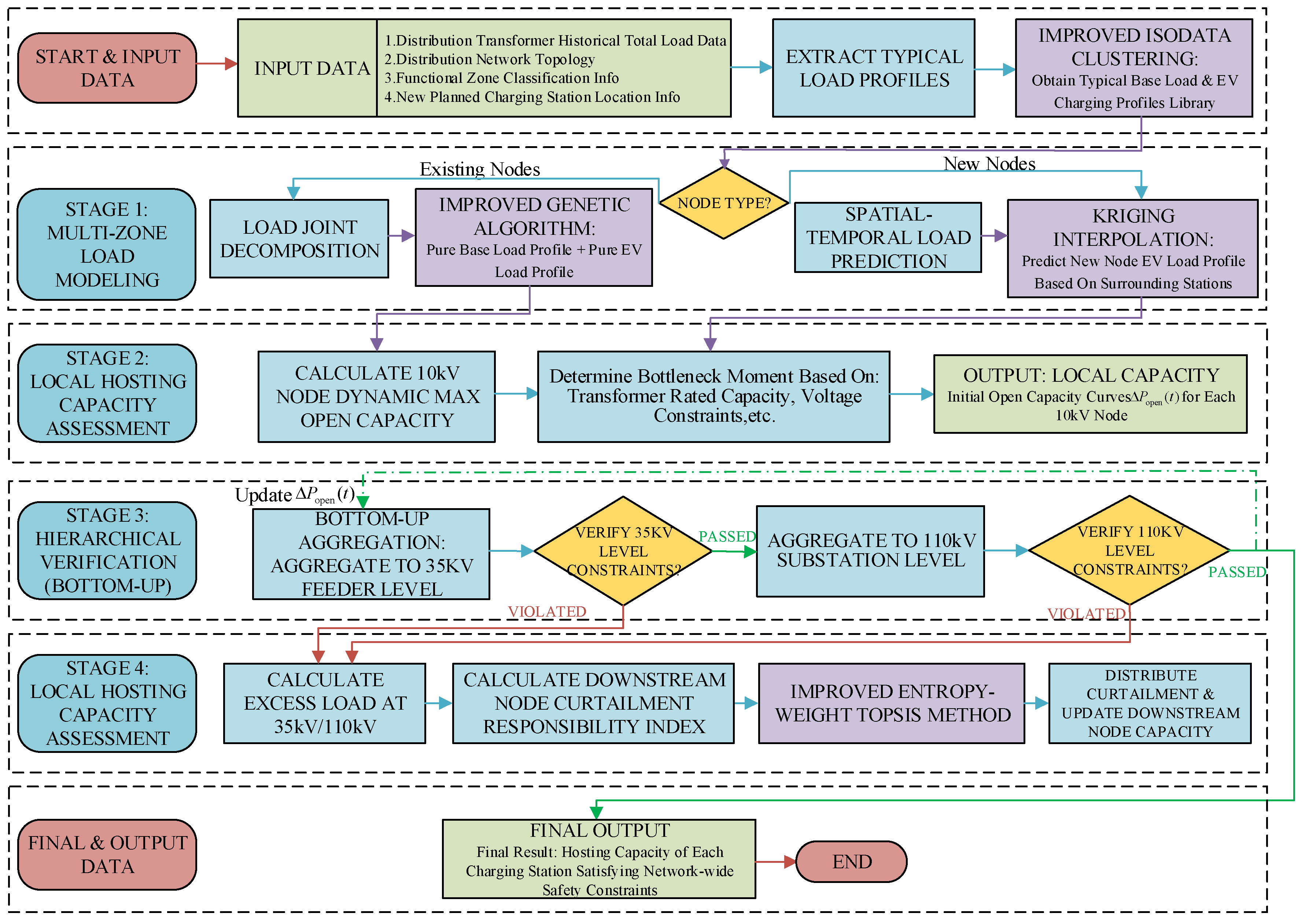
The final stage evaluates capacity along the Transformer-Feeder-Substation hierarchy. Open HC is first calculated for each 10 kV node. The corresponding load effects are then accumulated to the 35 kV and 110 kV levels. If an upstream constraint is exceeded, the improved EW-TOPSIS model assigns the required curtailment among downstream nodes according to zone attributes, load volatility, and regional operating pressure. Thus the reported HC is not only locally feasible; it also satisfies the upstream constraints that would be seen by the operating utility. Figure 2 shows the complete procedure from data input to capacity output.

2.2. Multi-Zone Load Profiling and Joint Decomposition

2.2.1. Improved ISODATA-Based Typical Load Profile Clustering

Clustering is used to build a compact library of daily load shapes for residential, commercial, and public-service zones. In the conventional ISODATA process, candidate cluster centers are set first. Each daily curve is then assigned to the closest center, usually measured by Euclidean distance, and the assignment is updated iteratively.
D x , z j = x z j 2
where x represents an individual daily load curve vector (e.g., 96 points for 15 min intervals), and z j the centroid vector of the j -th cluster.
After each assignment, the center of a cluster is recalculated from the samples allocated to it. The dispersion of the samples is checked at the same time. When the largest component of the deviation vector is greater than the splitting threshold, the cluster is considered to contain more than one operating pattern and is divided so that those patterns can be represented separately.
z j = 1 N j x S j x z j ± = z j ± 0.5 · σ j , m a x
where N j denotes the number of samples currently assigned to cluster j , and S j is the set of all such samples.
The reverse step is also necessary. Distances between cluster centers are checked to remove redundant scenarios. If two centers are closer than the merging threshold, they are merged into one center, with the sample counts of the original clusters used as weights.
z n e w = N i z i + N j z j N i + N j
Euclidean distance by itself is not a good fit for daily load curves. Two curves can have similar magnitudes but still differ in peak timing or short-term fluctuations. The improved ISODATA method therefore changes the standard procedure in two ways. It uses a more reliable initialization scheme for the cluster centers and replaces the original distance measure with a kernel-induced metric.
For initialization, the Max-Min distance rule is used to keep the initial centers separated in the sample space. This reduces the influence of random starting points and usually shortens convergence. Because load curves have nonlinear shape features, a kernel mapping is then introduced so that similarities in profile shape can be measured in a transformed feature space rather than only in the original coordinate space.
K x , z = λ k α x , z + c d + 1 λ k e x p x z σ k
where x represents the load sample vector and z represents the cluster centroid; x , z denotes the inner product; d is the degree of the polynomial kernel, controlling the extraction of global shape features; λ k [ 0,1 ] is a weighting coefficient that balances the contribution of the polynomial kernel and the exponential kernel.
Accordingly, the distance D ( x , z ) between a sample x and a centroid z in the high-dimensional feature space is defined as
D x , z = K x , x 2 K x , z + K z , z
Using the kernel-induced distance in the assignment and splitting operations makes the clustering more sensitive to curve shape. This is important for EV and base-load profiles, where the time of the peak and short local variations can be more informative than the daily amplitude alone.
In this study, the improved ISODATA process is implemented as follows. Each daily curve is normalized before clustering, so the comparison emphasizes the shape of the 24 h profile. The Max-Min rule chooses the starting centers, samples are allocated by the kernel-induced distance, and each center is recalculated from the samples assigned to it.
Very small clusters are removed because they usually reflect accidental or noisy operating days rather than stable scenarios. A cluster is split when its internal spread is too large, and two clusters are merged when their centers become nearly identical. The merged center is weighted by the number of samples in the two original clusters.
The parameters define how detailed and stable the profile library will be. The expected cluster number controls the target size of the library. The minimum sample size filters isolated abnormal curves. The splitting and merging thresholds decide whether a pattern should be separated or combined. The merge limit prevents excessive structural changes during one iteration. The iteration ends when the cluster structure no longer changes materially or when the maximum number of iterations is reached. The output is a set of representative profiles for residential, commercial, and public-service loads, which are then used in decomposition and HC assessment.

2.2.2. Improved GA-Based Load Decomposition Model

User-side charging records are not directly linked with distribution-station measurements in the studied system. As a result, the EV charging component has to be inferred from the aggregate transformer curve. The decomposition model treats the measured total load as a weighted combination of typical EV profiles and typical base-load profiles at each time step.
P e v t , X = w e v · P c h a r t P o t h t , X = w o t h · P o t h t
where P c h a r t and P o t h t denote the typical load profiles for EV charging and base loads at time t , respectively, while w e v and w o t h are their corresponding weight coefficients to be optimized.
The search begins with a standard genetic algorithm. Each individual in the population represents one feasible set of EV and base-load profile weights within [0, 1]. The objective is to make the reconstructed curve as close as possible to the measured transformer curve. The fitness value is therefore derived from the inverse of the reconstruction error.
f i t n e s s X = 1 1 + S S E X S S E X = t = 1 T P t o t a l t P e v t , X + P o t h t , X 2
where SSE(X) is the squared-error total between the measured transformer load P t o t a l t and the load reconstructed from the selected profile weights; it is used to define the fitness indicator f i t n e s s X . A larger fitness value therefore means that the decomposed EV and base-load profiles reproduce the measured curve more closely.
A standard GA may converge to a local solution when several profile-weight combinations give similar errors. To reduce this risk, the IGA adds a Levy-flight perturbation after the ordinary mutation operation. Levy flight has a heavy-tailed step-length distribution, so most steps remain local while occasional larger jumps help the population leave a narrow search region.
X n e w = X o l d + α L L e v y β
The perturbation is generated with the Mantegna scheme. Gaussian random variables are used to construct the step length, allowing the search to alternate between local refinement and less frequent long-range exploration.
u N 0 , σ u 2 , v N 0 , σ v 2 σ v = 1 , σ u = Γ 1 + β s i n π β / 2 Γ 1 + β 2 β 2 β 1 / 2 1 / β s = u v 1 / β
where σ v = 1 indicates that v follows a standard normal distribution, β is the shape parameter of the Levy distribution with a value range of β ( 1,2 ] , Γ ( · ) denotes the Gamma function which is mainly used to describe the probability density characteristics of random variables, and s represents the step length of Levy flight.
The decomposition procedure can be read directly from the chromosome structure. A chromosome stores one candidate vector of profile weights. For that vector, the transformer load is reconstructed by summing the weighted EV and base-load profiles, and the SSE between the reconstructed and measured curves is used as the objective value.
During iteration, individuals with smaller reconstruction errors are more likely to survive into the next generation. Crossover and mutation generate new feasible weight combinations, while elite retention ensures that the current best solution is not lost. After mutation, Levy-flight perturbation is applied to part of the offspring so that the population does not become trapped in a narrow region of the search space when different weight combinations produce similar aggregate curves.
The IGA settings include population size, the maximum number of iterations, crossover probability, mutation probability, the elite-retention ratio, the Levy step coefficient, and the convergence tolerance. Population size and iteration number mainly affect search depth and computational cost. The elite ratio determines how much protection is given to strong solutions, the Levy coefficient sets the strength of long-range exploration, and the convergence tolerance stops the search when the SSE changes only marginally. After convergence, the EV component is reconstructed from the optimized EV-profile weights, while the remaining weights represent the base-load component.
This design improves the chance of escaping local attraction regions. Once the algorithm converges, the separated EV charging load is obtained as
P e v * t = w e v , o p t · P c h a r t
where w e v , o p t is the optimal weight vector obtained after convergence, and P e v * t is the final estimated EV charging load profile.
Pseudocode: Improved GA with Levy Flight
Input:   Total   load   data   P t o t a l ( t ) ,   typical   load   profiles   ( P b a s e ( t ) ,   P c h a r ( t ) ) ,   population   size   N ,   max   iterations   G m a x ,   parameters   β ,   α L ;
Output:   Optimal   EV   load   decomposition   weight   w e v , o p t ;
  • Population   Initialization :   Generate   N   EV   load   weight   individuals   X i = [ w e v , i ] ( w e v , i [ 0,1 ] );
  • Calculate fitness of each individual (based on load estimation error);
  • Record   initial   optimal   individual   X b e s t   and   corresponding   fitness   F b e s t ;
  • Iterative   Optimization :   While   ( iteration   g G m a x and not converged);
    4.1
    Selection: Generate parent population via binary tournament selection;
    4.2
    Crossover: Perform arithmetic crossover on parent individuals to generate offspring;
    4.3
    Mutation: Execute Gaussian mutation on offspring, constrain weight range;
    4.4
    Levy Flight Perturbation: Apply Levy flight perturbation to mutated individuals, update positions;
    4.5
    Elitism: Retain current optimal individual in the next-generation population;
    4.6
    Update   population   fitness   and   global   optimal   individual   X b e s t ;
    4.7
    Iteration   count   g = g + 1 ;
  • Output   optimal   weight   w e v , o p t = X b e s t .

2.2.3. Spatial-Temporal Prediction of Charging Load for New Stations

HC assessment for planned EVCSs requires a charging profile before the station has operated. The assumption used here is that stations in the same functional zone share a spatial relation in travel demand and charging behavior. Kriging interpolation is therefore used to infer the profile composition of a new station from the weights observed at nearby stations.
The procedure first selects existing stations in the target functional zone as samples. Each sample station is represented by its coordinates and by a vector of typical-profile weights. The vector shows the contribution of each profile to the station load, and the components satisfy the normalization constraint.
For a planned station, OK interpolation is performed separately for every profile-weight component. For one given profile, the known weights at existing stations form the observations used to estimate the unknown weight at the new location.
γ h = 0 h = 0 N 0 + P s 3 h 2 a 1 2 h a 3 0 < h a N 0 + P s h > a
Spatial dependence is described by a semivariogram. The model relates the variance of the weight difference to the distance between stations. A spherical semivariogram is adopted because it can represent both near-distance correlation and the range beyond which correlation becomes weak.
The Kriging weights of the known stations are obtained by solving the OK system. Under the selected semivariogram, this gives an unbiased estimate with minimum estimation variance.
j = 1 m λ j γ h i j + μ = γ h i 0 , i = 1 , , m i = 1 m λ i = 1
In the OK system, terms built from distances among existing stations describe the relation within the sample set. Terms involving the planned station describe its relation to those samples. The Lagrange multiplier is used to satisfy the unbiasedness condition.
After the system is solved, the estimated components form the profile-weight vector of the planned station. The vector is normalized so that the synthesized load curve keeps a physically interpretable profile composition.
w ^ j = w ^ j k = 1 K N w ^ k
The daily charging curve of the planned station is finally obtained by combining the typical profiles according to the estimated weights and scaling the result by the station capacity.
P n e w t = n c h a r g e r s × j = 1 K N w ^ j × P j t
where P j t is the normalized power curve of the j -th typical profile.
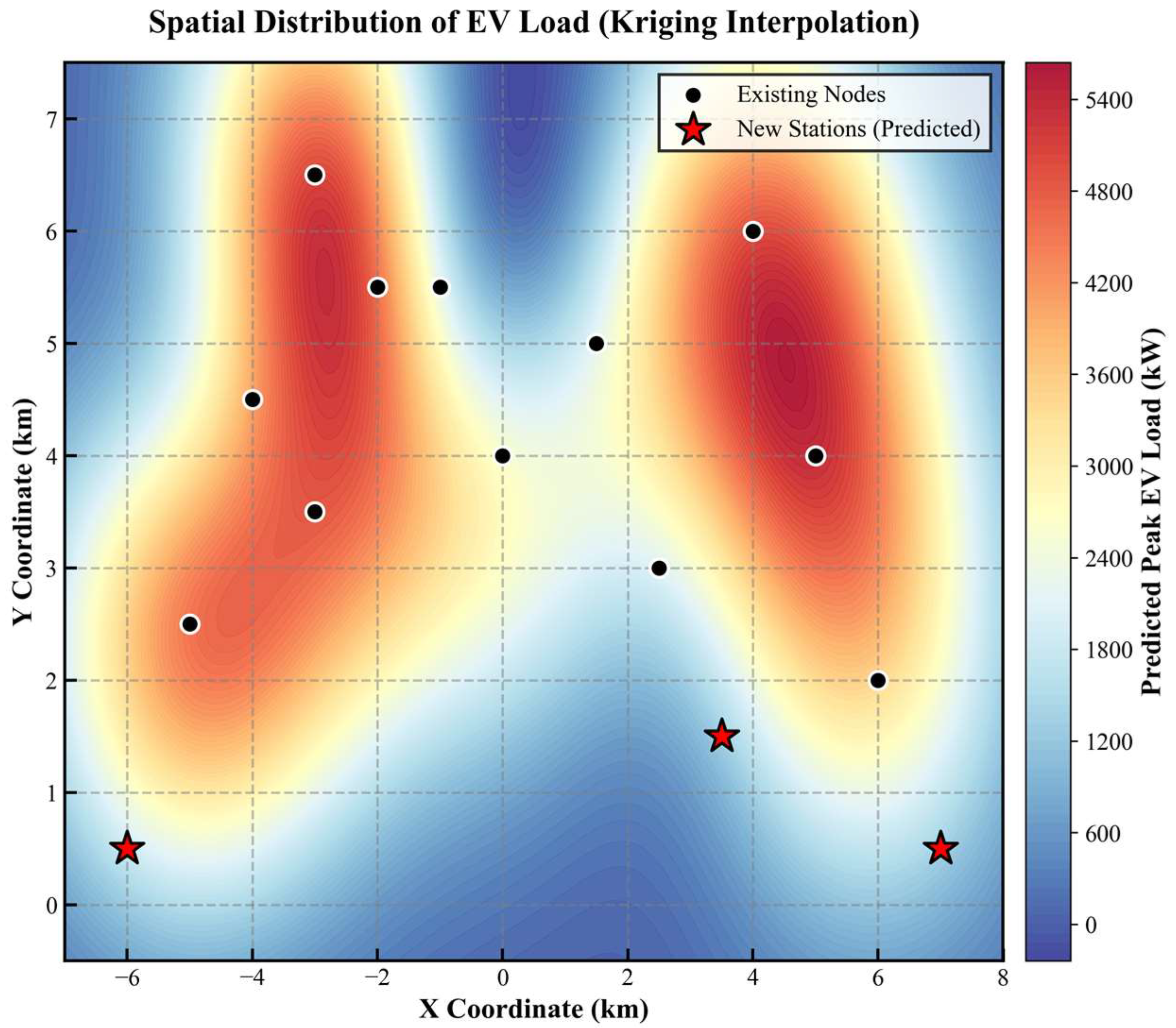
The OK prediction is illustrated for one functional zone in the test network. Figure 3 maps the predicted peak EV charging load over the study area. Warmer colors correspond to larger predicted load intensity, while cooler colors indicate lower values. Existing charging stations are marked as training samples, and the planned stations are marked separately. The predicted surface follows the spatial distribution of the observed stations: areas closer to high-load samples receive larger estimated profile weights, whereas locations farther from those samples are assigned lower peak demand. This result shows how decomposed load information from monitored stations can be transferred to unmonitored EVCS sites before field measurements are available.

2.3. Calculation Method of Distribution Network Hosting Capacity

2.3.1. Definition of Hosting Capacity and Operational Constraints

HC is defined as the largest additional EV charging load that can be connected without violating operational limits. In this paper it is treated as a time-dependent quantity, because the limiting margin changes with topology, background demand, and the daily shape of EV charging.
S t o t a l t = P b a s e t + P E V t 2 + Q b a s e t + Q E V t 2 η · S r a t e d
where S r a t e d is the rated capacity, and η is the allowable loading factor.
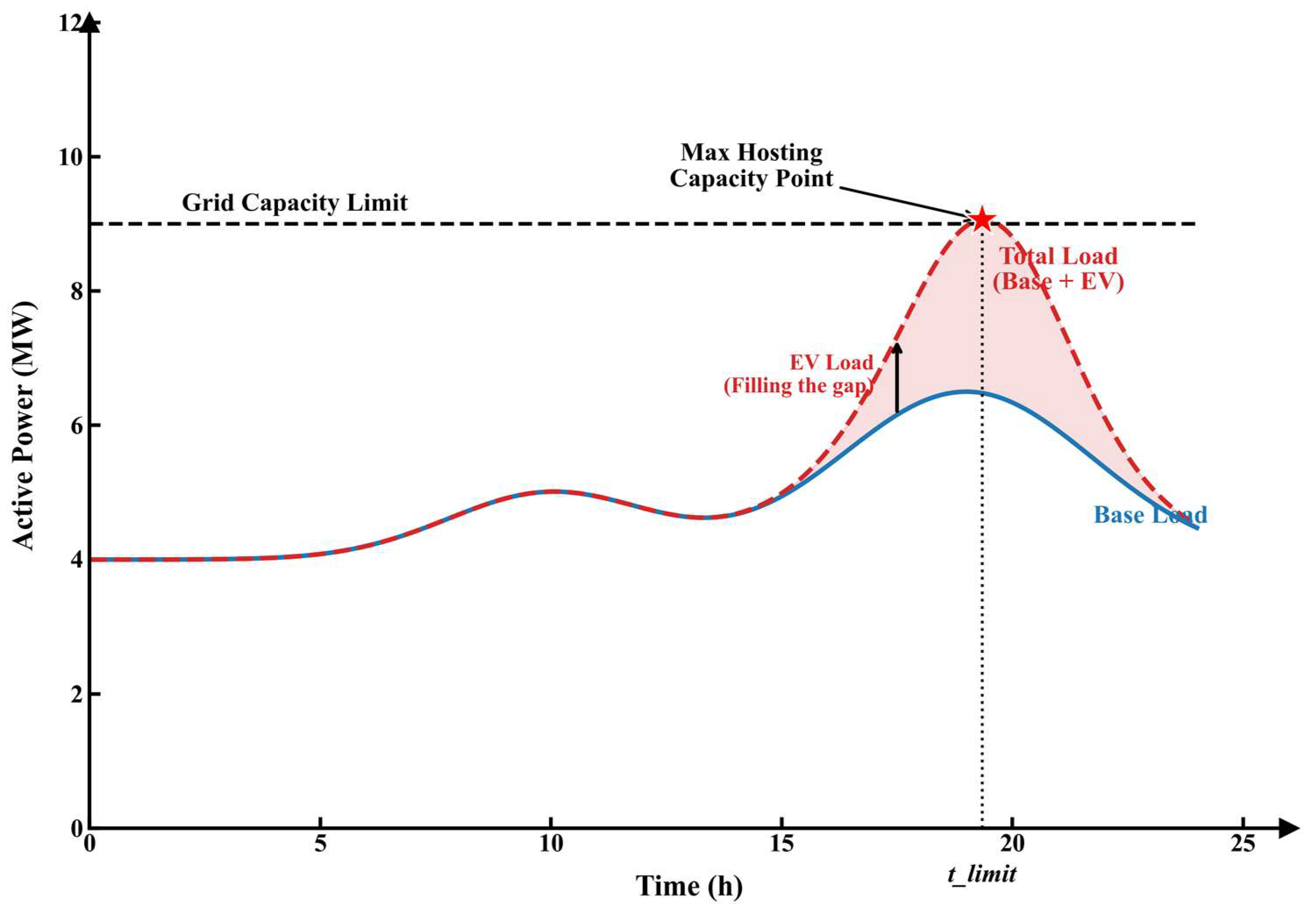
Figure 4 explains the calculation concept. The background load and the incremental EV charging profile are superimposed and compared with the active capacity boundary. As the EV demand is scaled upward, the first time point at which the total curve reaches the boundary becomes the bottleneck. The corresponding EV load level is taken as the HC, and any further increase would violate the operating constraint.

2.3.2. Calculation Algorithm of Hosting Capacity

Open HC is calculated as a time-series constrained optimization problem. The aim is to determine the largest additional EV charging load that a transformer can carry over the whole scheduling horizon. Because both background demand and EV charging vary during the day, the calculation must identify the most restrictive interval rather than only the daily peak of one curve.
At each time step, the available power margin is calculated first. This margin is the spare transformer capacity after supplying the current total load, including base demand and the EV load that already exists at the node.
P m a r g i n t = η · S r a t e d P t o t a l t , t T
where P m a r g i n t denotes the available power margin at time t , and S r a t e d is the rated transformer capacity used in the local constraint. The coefficient η reserves operating headroom, so the calculation keeps a practical safety allowance instead of using the full nameplate rating. P t o t a l t is the current nodal load curve obtained after the decomposition of the measured transformer load.
The typical EV charging profile from Section 2.2.1 is then compared with the available margin at each time step. The ratio gives the expansion factor that would be feasible at that moment.
k t = P m a r g i n t P e v t
where k t is the feasible expansion factor for the evaluated time step, and P e v t is the normalized EV charging profile selected for the corresponding functional zone.
The global expansion coefficient is the minimum of the time-varying ratios. This minimum identifies the bottleneck moment, when the network is most stressed relative to the added EV load. The final HC curve is obtained by multiplying the typical EV profile by this limiting coefficient.
K o p e n = m i n t T k t Δ P o p e n t = K o p e n · P e v t
Thus, one bottleneck interval determines the maximum additional EV load curve that can remain feasible for the entire day.
This calculation gives the maximum connectable charging capacity at the local transformer while preserving the temporal relation between background load and EV demand. Local feasibility is not enough, however, because several locally feasible stations may still create an upstream violation after aggregation.

2.4. Hierarchical Verification and Capacity Reallocation

2.4.1. Bottom-Up Aggregation Strategy

The distribution network is organized hierarchically: power is supplied from high-voltage substations to feeders and then to low-voltage transformers. The HC obtained in Section 2.3 protects each local transformer, but the simultaneous operation of several downstream EVCSs may overload a 35 kV feeder or a 110 kV substation. A bottom-up aggregation step is therefore added.
For a 35 kV feeder node k , the aggregated demand curve P d e m a n d , k t is assembled from three parts: downstream EV-node HC, base load from non-EV nodes, and any industrial load directly connected to the 35 kV bus. This form keeps the EV expansion load, ordinary demand, and direct industrial demand visible in the same feeder-level curve. The relation is expressed as
P d e m a n d , k t = i Ω E V , k Δ P o p e n , i t + j Ω p u r e , k P b a s e , j t + P i n d , k t
where the first set denotes downstream 10 kV EVCS nodes connected to the feeder, and the second set denotes downstream pure-load nodes without EV facilities. The EV-node term uses the HC curve calculated in Section 2.3, the pure-load term uses the corresponding base-load curve, and the industrial term represents the load directly connected to the 35 kV bus.
At the 110 kV level, feeder demands are accumulated in the same manner. Let m denote a 110 kV node; its aggregated demand P d e m a n d , m t is obtained by summing the demand curves of all subordinate 35 kV feeders connected to that substation k .
P d e m a n d , m t = k Ω 35 k V , m P d e m a n d , k t
where Ω 35 k V , m represents the set of 35 kV feeders connected to the 110 kV substation m .
This aggregation describes the most demanding plausible condition at each voltage level, because all downstream EVCSs are assumed to operate at their open HC at the same time. It is used to test whether local capacity decisions remain feasible when observed from the upstream grid.

2.4.2. Constraint Verification

After aggregation, each voltage level is checked against its own capacity limit. The verification moves from the lower level to the higher level so that an overload can be traced to the downstream nodes that contribute to it.
P d e m a n d , k t ρ 35 k V · C r a t e d , k , t T
If the inequality is satisfied at every time step, the feeder is secure. If demand exceeds the limit, a violation is recorded for the corresponding period. The resulting excess load Δ P e x c e s s , k t is calculated as
Δ P e x c e s s , k t = m a x 0 , P d e m a n d , k t ρ 35 k V · C r a t e d , k
If Δ P e x c e s s , k t is positive, the 35 kV feeder has a capacity bottleneck, and the open capacities of its downstream EV stations must be reduced. The 110 kV verification follows the same logic: aggregated feeder demand is compared with the substation’s rated capacity after applying the safety coefficient ρ 110 k V to identify the magnitude and timing of any remaining overload Δ P e x c e s s , m t .
The hierarchical check ensures that the final HC result satisfies the admissible constraints of each voltage layer. It also identifies the overloaded period and the location where adjustment is required, which provides the input for targeted reallocation.

2.4.3. Capacity Reallocation Strategy Based on Improved EW-TOPSIS

When an upstream node violates its capacity limit, part of the open HC assigned to downstream EVCSs must be withdrawn. This paper treats that withdrawal as a multi-criteria allocation problem and solves it with the improved EW-TOPSIS model.
For the downstream EV nodes connected to the overloaded upstream node, three indicators are used to construct the evaluation matrix:
  • Functional Zone Priority ( f 1 ) : This indicator reflects the social importance and demand rigidity of the served zone. Residential zones, which correspond more closely to basic livelihood needs and usually have lower elasticity, are assigned higher protection priority. Commercial zones, which generally have stronger regulation potential and demand-response capability, can tolerate larger curtailment ratios under capacity constraints.
  • Load Fluctuation Coefficient ( f 2 ): This indicator measures the stability of the node HC profile and is calculated as the ratio of the standard deviation to the mean of the capacity curve. Smaller fluctuation indicates a more stable and predictable load resource.
  • Regional Industrial Load Peak ( f 3 ): This indicator represents the peak industrial demand of the 35 kV region where the node is located. Nodes in regions with heavier industrial loading may receive stronger curtailment pressure to relieve regional stress.
The initial decision matrix is built from these three indicators. The matrix is normalized with the min-max method to remove dimensional inconsistency, and the indicator weights are calculated by the entropy-weight method instead of being set manually.
E j = k e i = 1 m p i j ln p i j w j = 1 E j k = 1 3 1 E k
where p i j = x i j i = 1 m x i j is the proportion of the indicator value, and k e = 1 l n ( m ) .
The normalized matrix is multiplied by the entropy-derived weight vector to obtain the weighted matrix. Positive and negative ideal solutions are defined from the best and worst column values. The distance from each node to these two solutions is then calculated, and the relative closeness coefficient is used as the comprehensive score.
D i + = j = 1 3 Z i j Z j + 2 D i = j = 1 3 Z i j Z j 2 C i = D i D i + + D i
A larger closeness coefficient means that the node should be protected more strongly, for example because it serves a higher-priority zone or has a more stable capacity profile. Capacity reduction is therefore assigned inversely to this coefficient.
The total excess load is then distributed among the downstream nodes according to these scores, and the optimized HC of each node is updated.
Δ P r e d , i = Δ P e x c e s s · C i k = 1 m C k Δ P f i n a l , i = Δ P i n i t , i Δ P r e d , i
The reallocation strategy changes curtailment from a uniform technical reduction into a decision process that considers service priority, load stability, and regional pressure at the same time. The resulting capacities remove the upstream violation while keeping the 10 kV, 35 kV, and 110 kV constraints consistent.

3. Case Studies

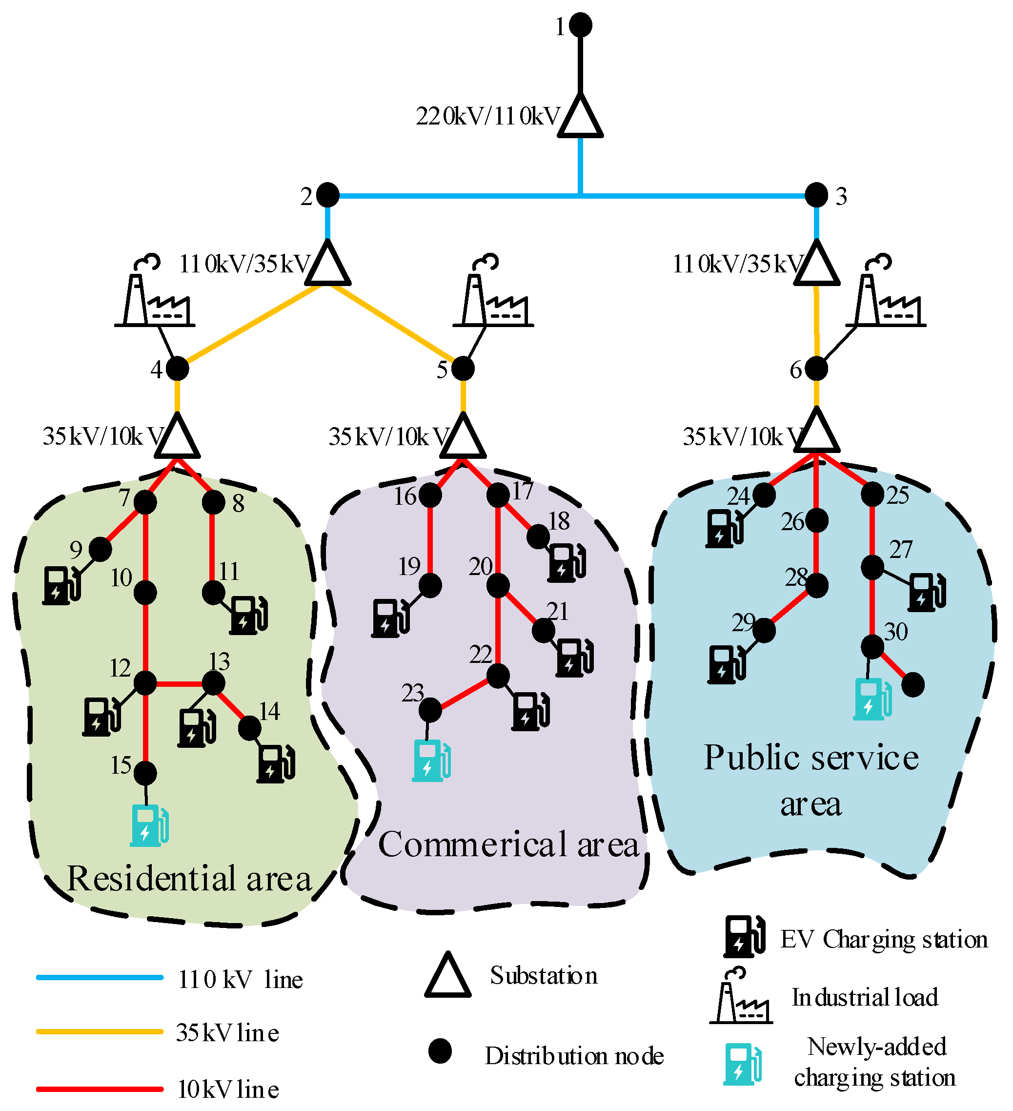
A modified regional distribution network is used to test the hierarchical HC framework. As shown in Figure 5, the system follows a 220 kV/110 kV supply, 110 kV/35 kV substations, and 35 kV/10 kV distribution transformers. Three 110 kV/35 kV substations supply residential, commercial, and public-service zones through 35 kV lines. The 35 kV/10 kV transformers at Nodes 4, 5, and 6 represent the three functional zones. Large industrial loads are connected directly to the 35 kV buses so that the influence of high-voltage industrial users on regional capacity can be examined. EVCSs are assigned to several 10 kV nodes, including both existing stations and planned expansion sites. Table 2 gives the hyperparameter settings used in the case study.
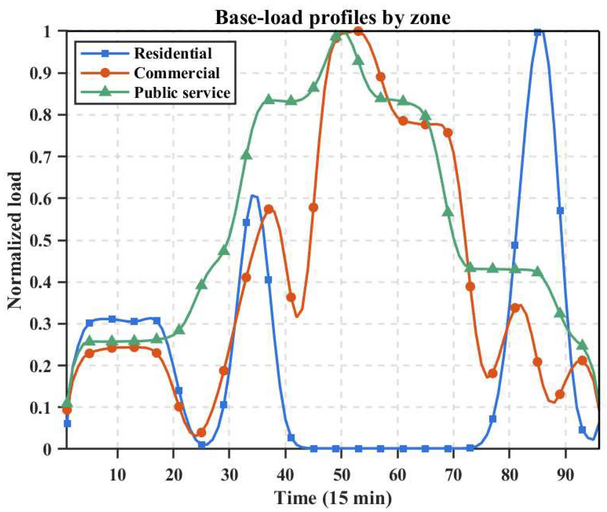
The historical load dataset was processed with the improved ISODATA method in Section 2.2.1 to obtain representative regional load patterns. Because the method splits and merges clusters during iteration, it can adjust the number of daily scenarios rather than forcing all days into a fixed number of groups. Figure 6 shows the typical base-load profiles of the three functional zones. The residential profile has a morning shoulder and a stronger evening peak. The commercial profile remains high during business hours and falls after work. The public-service profile is more stable during the daytime. These different shapes imply that each zone has a different time window in which EV integration becomes difficult.
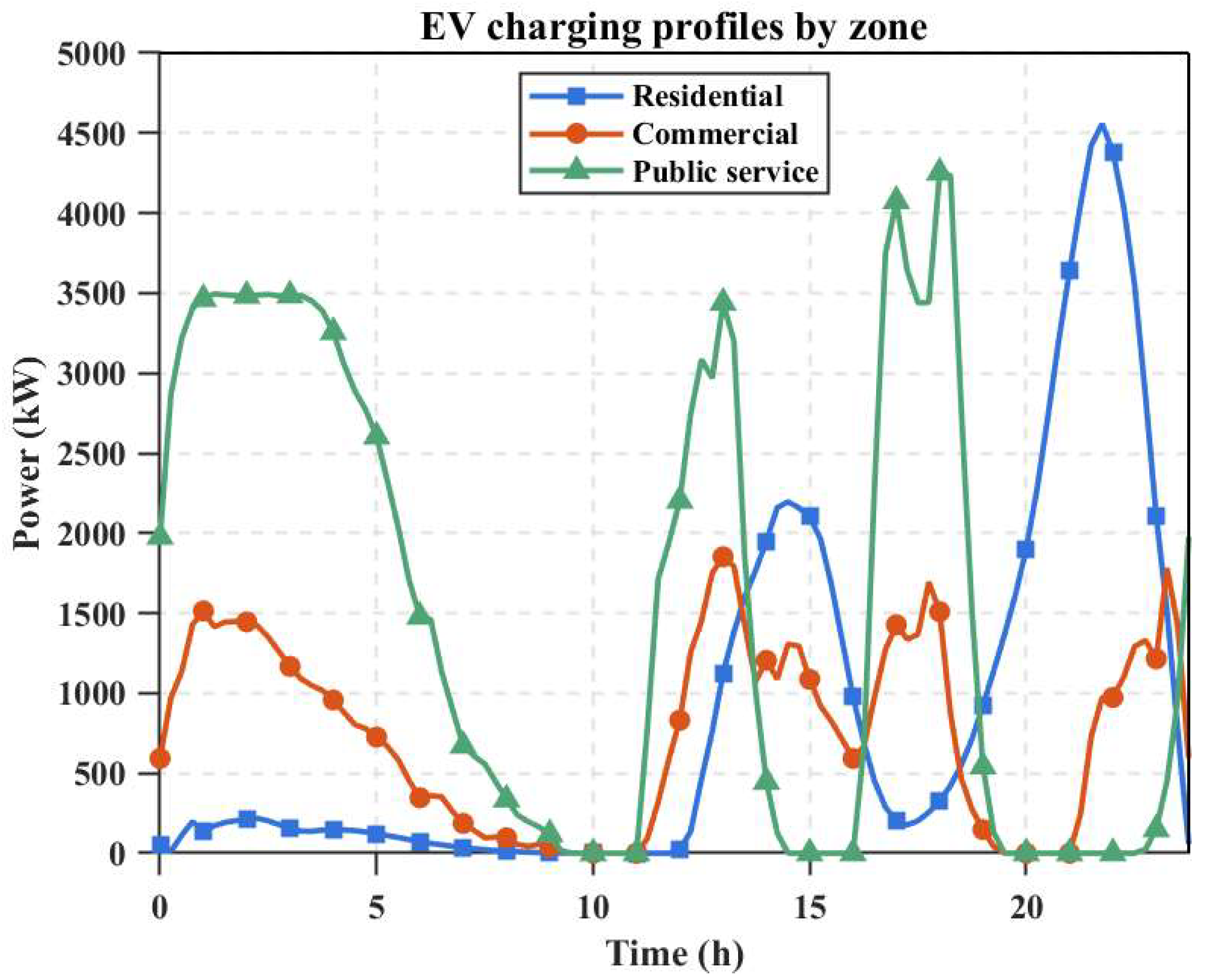
Figure 7 shows that the EV charging profiles are also zone dependent. Residential charging increases rapidly after 18:00, when users return home, and it overlaps with the residential base-load peak. Commercial charging mainly occurs during working hours and is added to an already high commercial plateau. Public-service charging has sharper daytime fluctuations and larger short-term peaks. Because the EV profile interacts differently with the base load in each zone, a dynamic time-series HC calculation is needed to locate the true bottleneck period.
In the tested distribution network, operators observe the total transformer load rather than separate EV and base-load components. Before HC is calculated, the IGA model in Section 2.2.2 is therefore applied with the ISODATA profiles as basis vectors.
The decomposition is solved as a profile-weight optimization problem. The model searches for the set of weights whose linear combination best matches the measured total load curve. Elite retention keeps the best individuals between generations, and the adaptive stopping rule ends the search if the fitness remains unchanged for 100 consecutive iterations. These settings are used to improve stability without unnecessarily increasing the calculation time.
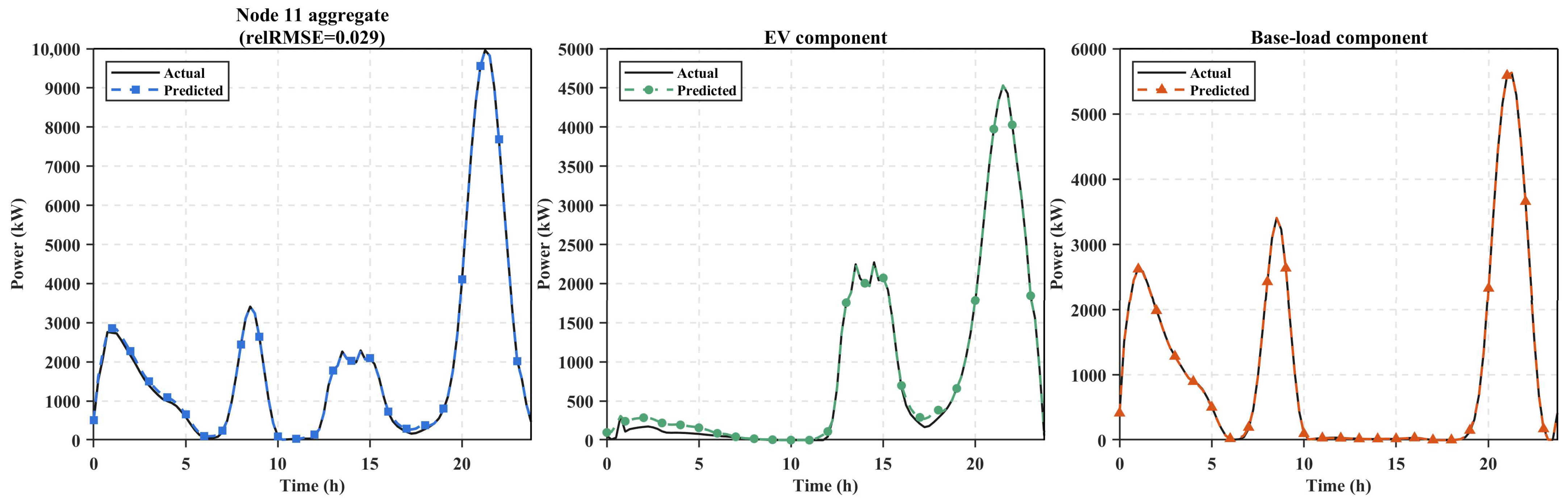
Figure 8 gives the result for Node 11, a representative residential node. The measured total load has two peaks, with the larger one around 20:00. The separated EV component is small during the daytime and rises quickly after 18:00, reaching its maximum close to the residential base-load peak. This pattern indicates that home charging is the dominant EV demand at this node. The reconstructed total load follows the measured curve closely, so the decomposition captures the evening bottleneck that controls the node capacity.
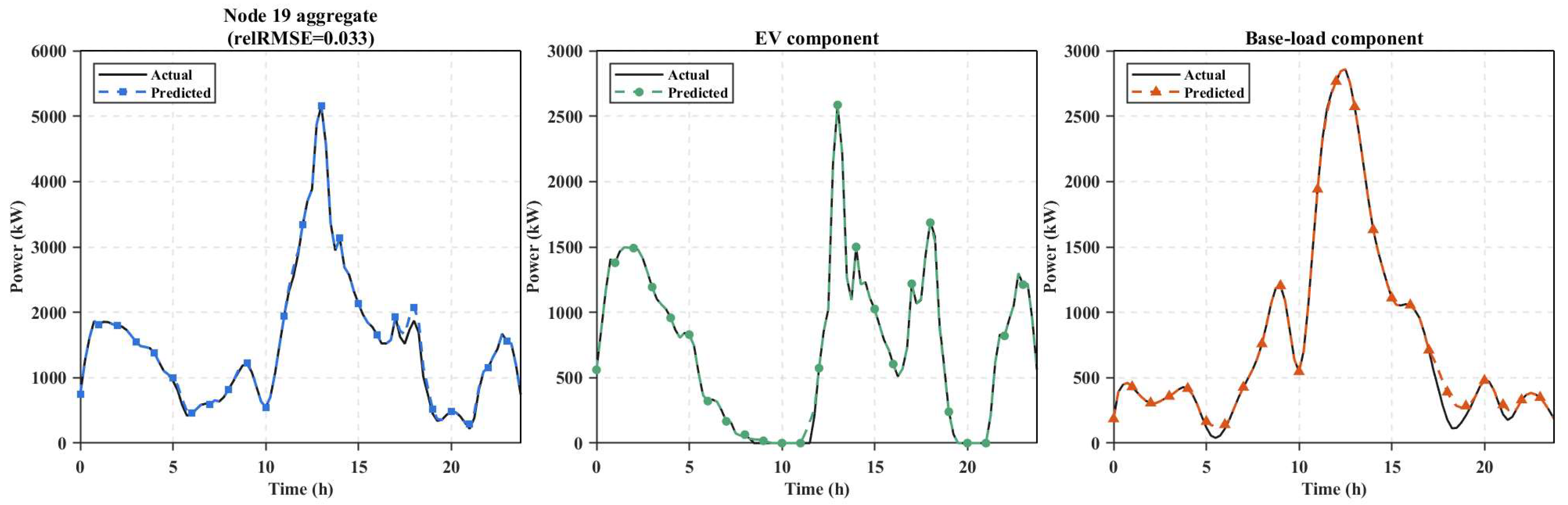
The commercial-zone case is represented by Node 19 in Figure 9. Its EV component is concentrated from about 09:00 to 18:00 and overlaps with the high commercial base-load plateau. The main capacity pressure is therefore a daytime problem rather than an evening problem. The improved GA separates the variable EV component from the steadier commercial background load, which provides the load input needed for transformer-level HC assessment.
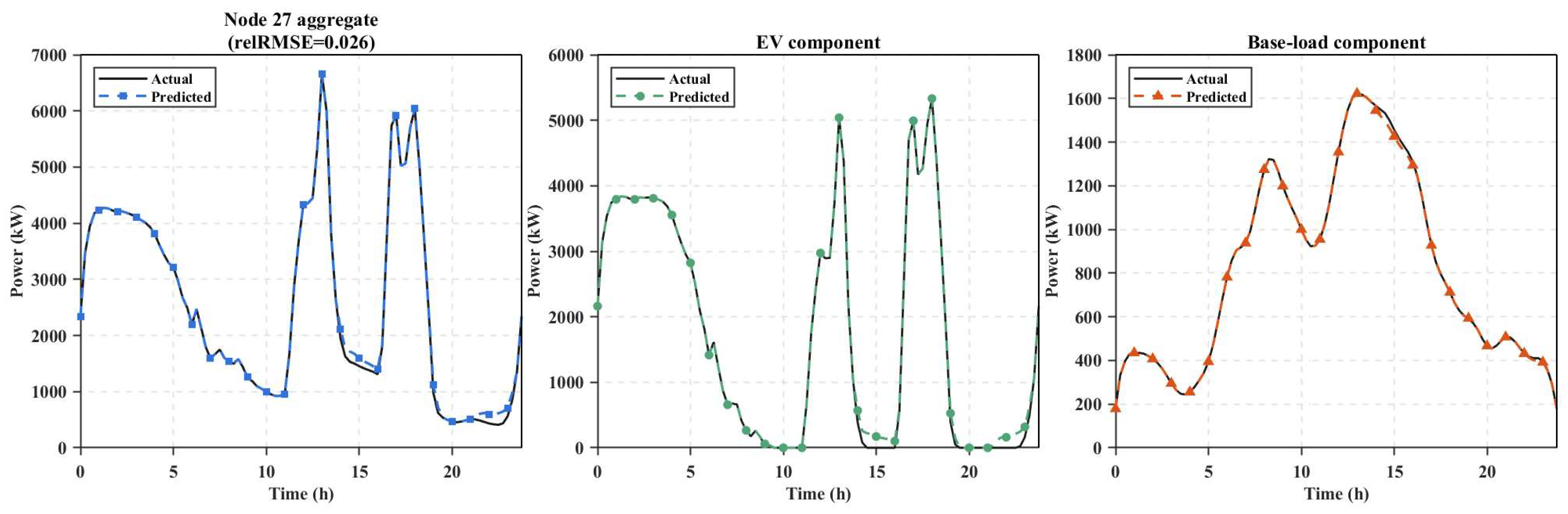
Node 27 in the public-service area is shown in Figure 10. The total load curve is irregular, and the separated EV component accounts for most of the sharp spikes. This behavior is consistent with high-power fast charging by buses, taxis, or other public-service vehicles. The base-load component remains comparatively smooth, indicating that the model can still distinguish high-frequency charging variation from background demand in the most volatile zone.
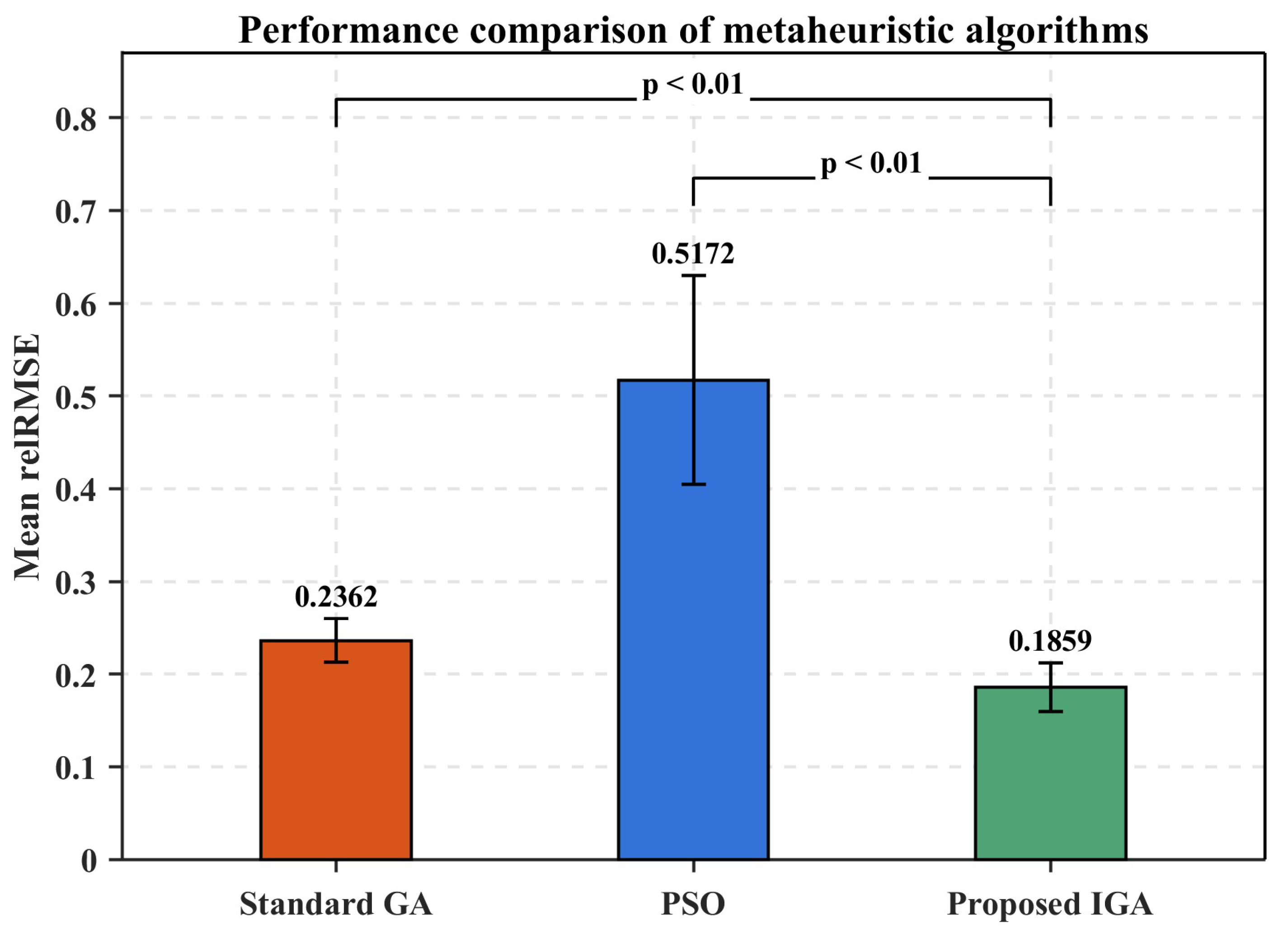
The optimization engine was evaluated separately by comparing standard GA, PSO, and the proposed IGA under the same decomposition objective. Twelve transformer nodes with nonzero EV charging components were used. Each algorithm was run 20 times with a population size of 60 and a maximum of 80 iterations.
Table 3 reports the lowest mean relative RMSE for the proposed IGA, 0.1859, compared with 0.2362 for standard GA and 0.5172 for PSO. The t-tests show significant differences from both benchmark algorithms (p < 0.01). These results support the use of IGA as the optimization engine in the load-decomposition stage.
Figure 11 compares the mean relative RMSE values of the three algorithms. The error bars show the standard error over repeated runs, and the significance brackets correspond to the t-test results. With the same objective function and parameter budget, IGA produces the lowest average error, which confirms its advantage for this decomposition task.
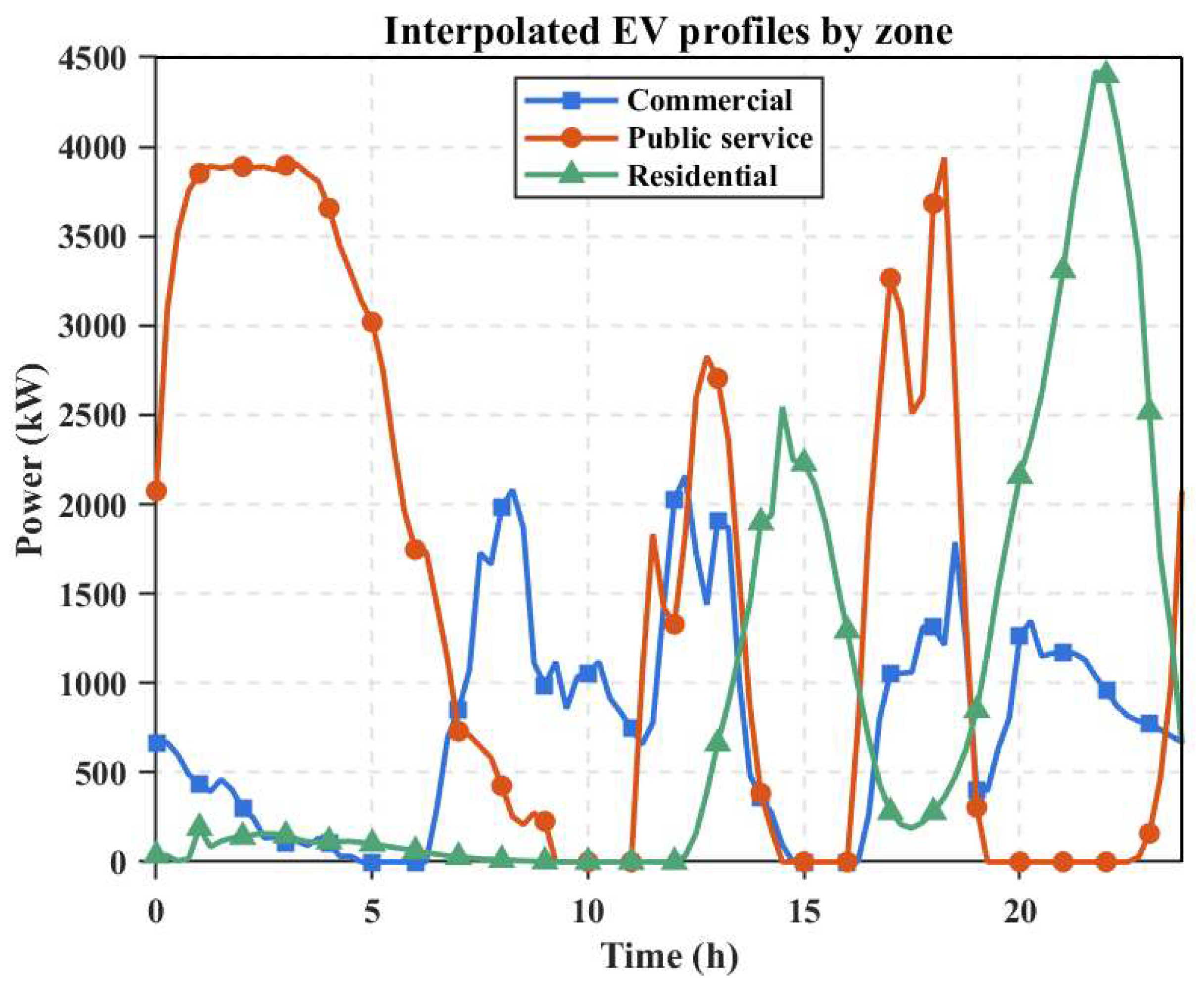
For planned EVCSs, no historical station measurements are available. The OK interpolation method is therefore used to estimate their profile weights from nearby observed stations. In this way, the EV load information separated from existing nodes is transferred to unobserved locations with similar functional-zone attributes. Figure 12 shows the predicted daily charging curves of the new stations.
The predicted curves retain the temporal characteristics of their zones. In the residential area, charging rises after 18:00 and peaks around 22:00, matching the home-charging pattern found at existing residential nodes. This indicates that the Kriging model preserves the spatial continuity of residential charging demand.
The commercial prediction remains active during business hours, with several peaks between 09:00 and 18:00. The public-service prediction has stronger daytime volatility and higher charging power, reflecting the rapid-charging behavior of public-transport-related demand. The separation among the three predicted curves provides usable input for HC calculation in the expanded network.
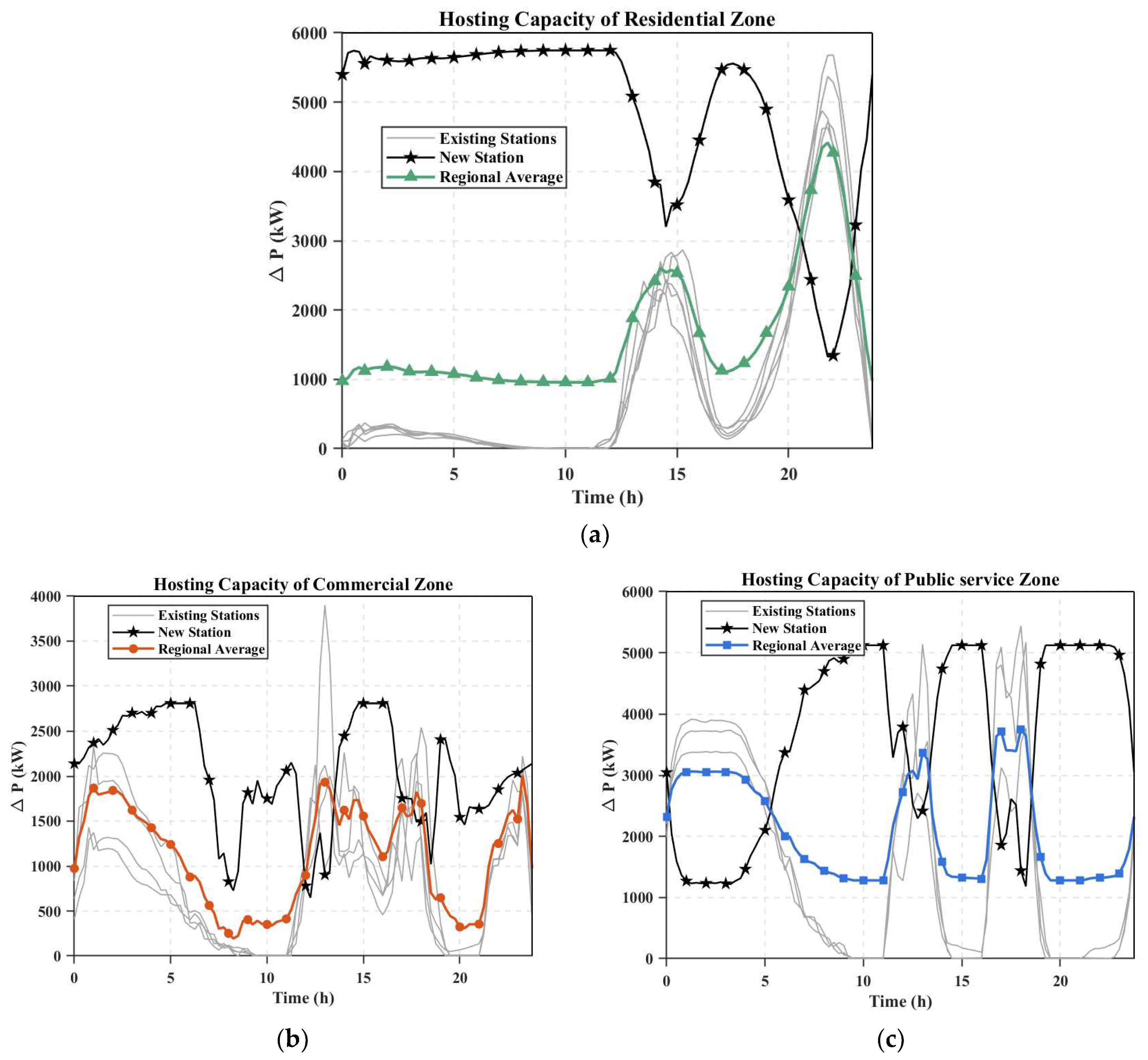
The dynamic HC of each node is calculated from the decomposed load components and the predicted profiles of new stations. The calculation follows the Shortest Stave principle: the admissible charging level is controlled by the smallest power margin over the day. Figure 13 presents the time-varying margins of individual nodes and zonal averages.
In the residential area, the available capacity is lowest during the evening peak, approximately 19:00–22:00. At this time, residential base load and home charging increase together. The result shows that evening coincidence is the main constraint on additional EV integration in residential feeders, so orderly charging or peak-shaving control should focus on this period.
The commercial area has a different constraint pattern. The capacity pressure is concentrated from about 10:00 to 16:00, and the margin remains low for a longer period because the commercial base load stays high through the workday. The bottleneck is broader than in the residential zone, even though the instantaneous pressure is not always as severe.
The public-service area has the most volatile margin. Fast-charging demand changes quickly, and the minimum margin can approach zero during the day. This behavior suggests that simultaneous high-power charging events dominate the local HC limit. Storage, buffering, or charging-order control may therefore be especially useful at public-service stations.
The capacity curves of planned stations differ from those of existing mixed-load nodes. Planned stations are modeled as dedicated EV charging facilities connected to distribution transformers, while existing nodes also carry residential, commercial, or public-service background loads. Their HC is therefore mainly determined by transformer rating and predicted EV demand, not by the residual margin of a composite load curve. This difference is another reason to verify capacity hierarchically instead of estimating new-station capacity by averaging existing node behavior.
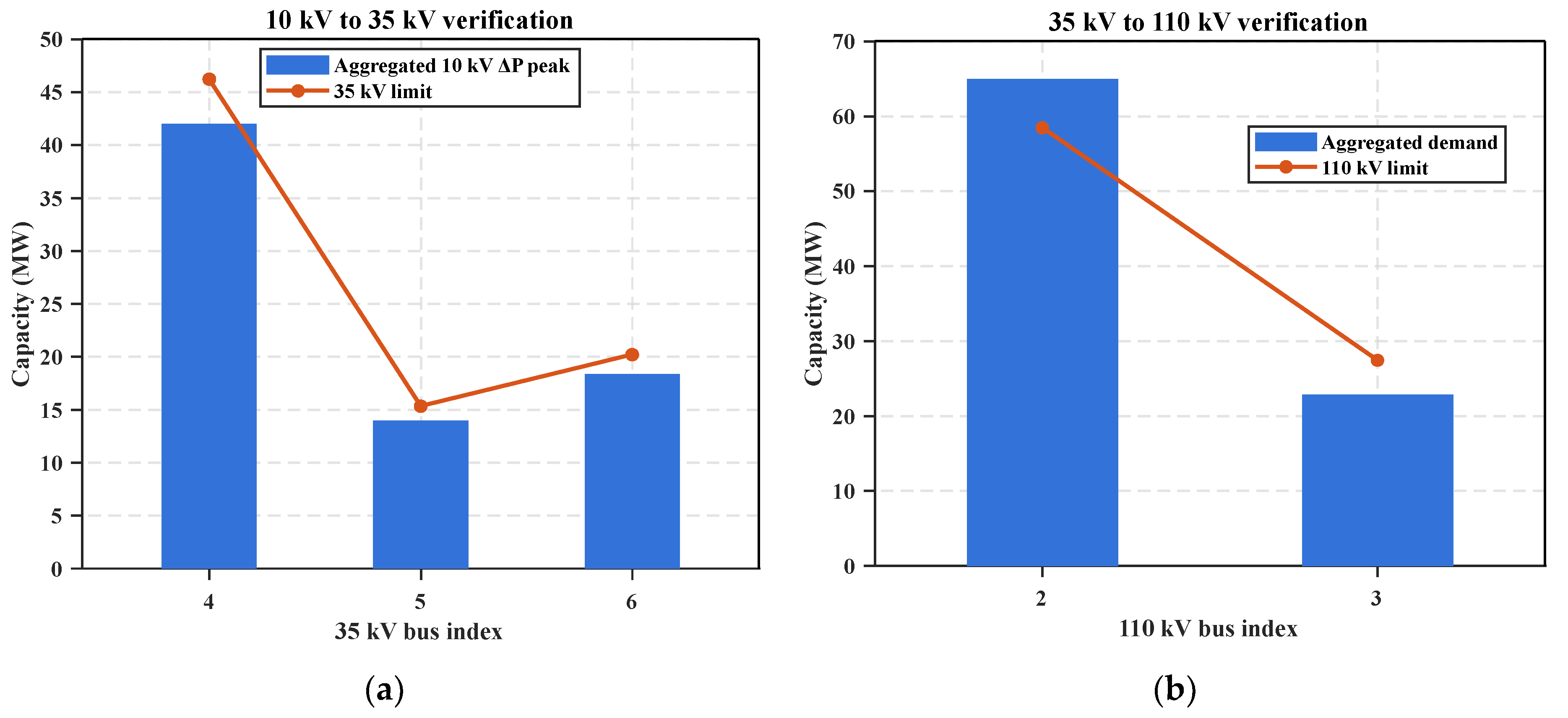
After the 10 kV node capacities are obtained, bottom-up verification is performed to check the upstream grid. Figure 14 summarizes the results at the 35 kV and 110 kV levels.
At the 35 kV level, the aggregated peak HC demands of the downstream nodes connected to Substations 4, 5, and 6 are 42.02 MW, 13.96 MW, and 18.38 MW. All three values remain below their transformer limits, so no congestion is detected at this level.
The 110 kV result is different. After the downstream loads are aggregated further, Substation 2 exceeds its limit: total demand reaches 64.98 MW, while the permissible value is 58.48 MW. Thus a set of stations that is feasible at the downstream level can still overload the superior node when residential and commercial peaks coincide. Capacity reallocation is required.
The improved EW-TOPSIS model is then activated to remove the overload at Substation 2. Each downstream node is evaluated by a Curtailment Responsibility Index that combines functional priority, load fluctuation, and regional impact. Table 4 lists representative reallocation results.
The reallocation results show a consistent pattern. Commercial nodes receive higher responsibility scores, generally between 0.83 and 0.90, because they have greater flexibility and lower livelihood priority than residential nodes. They therefore bear most of the curtailment. Node 22 has the largest reduction, 50.6%, and Nodes 18 and 21 also lose nearly half of their original capacity.
Residential nodes behave in the opposite way. Their responsibility scores remain near 0.16, so the model protects residential charging demand. Most residential reductions are about 4%, and Node 15, whose score is 0, keeps its original capacity. The allocation removes the upstream overload while preserving basic residential charging demand and assigning more adjustment to nodes with higher flexibility.

4. Conclusions

This paper proposes a hierarchical HC assessment method for EVCS planning in regional distribution networks. The method addresses three asymmetries that commonly arise in practice: charging demand varies across time and location, measurement availability is different on the user side and the transformer side, and spare capacity is uneven across voltage levels. It combines non-intrusive load decomposition, spatial interpolation, dynamic time-series verification, and differentiated reallocation to assess HC under limited observability.
The case study verifies that improved ISODATA and IGA can separate stochastic EV charging demand from aggregate transformer measurements. The separated profiles also show clear zone differences. Residential nodes are limited mainly by evening coincidence, while commercial nodes face a longer daytime constraint. OK interpolation transfers the observed spatial correlation to planned stations, reducing the dependence on local historical measurements.
The hierarchical verification results show that local HC is not sufficient as a final planning result. Even if all downstream nodes satisfy their own limits, the aggregated charging demand can still exceed the capacity of a 110 kV substation. Bottom-up verification is therefore needed to expose unequal margins across voltage levels and to keep local decisions consistent with upstream operation.
The improved EW-TOPSIS reallocation also allows the required adjustment to vary with zone priority and flexibility. Compared with uniform or proportional curtailment, it provides stronger protection for residential charging demand and places more adjustment responsibility on commercial nodes that can tolerate larger reductions. Future work will extend the method to distributed control and aggregator-based coordination so that large-scale EV charging can be managed under both symmetric and asymmetric decision settings.

Author Contributions

Conceptualization, N.G. and J.C.; methodology, J.C.; software, J.C.; validation, J.C.; formal analysis, N.G. and J.C.; investigation, X.Z. and J.L.; resources, Z.Z.; data curation, Y.C.; writing—original draft preparation, J.C.; writing—review and editing, N.G.; visualization, N.G.; supervision, N.G.; project administration, N.G.; funding acquisition, N.G. All authors have read and agreed to the published version of the manuscript.

Funding

This research was funded by the Science and Technology Project of Jiangsu Electric Power Test Research Institute Co., Ltd. (NO: DSY202509).

Data Availability Statement

Data are contained within the article.

Conflicts of Interest

The authors, Ning Guo, Jinming Chen, Xing Zhang, Ye Chen, Jian Liu, and Zhijun Zhou, were employed by Jiangsu Electric Power Test Research Institute Co., Ltd., Nanjing, China. The authors declare that this study received funding from the Science and Tech-nology Project of Jiangsu Electric Power Test Research Institute Co., Ltd. (NO: DSY202509). The funder was not involved in the study design, collection, analysis, or interpretation of data, the writing of this article, or the decision to submit it for publication.

References

  1. Mastoi, M.S.; Zhuang, S.; Munir, H.M.; Haris, M.; Hassan, M.; Usman, M.; Bukhari, S.S.H.; Ro, J.-S. An in-depth analysis of electric vehicle charging station infrastructure, policy implications, and future trends. Energy Rep. 2022, 8, 11504–11529. [Google Scholar] [CrossRef]
  2. Veldman, E.; Verzijlbergh, R.A. Distribution grid impacts of smart electric vehicle charging from different perspectives. IEEE Trans. Smart Grid 2014, 6, 333–342. [Google Scholar] [CrossRef]
  3. Imtiaz, S.; Yang, L.; Naz, M.N.; Munir, H.M.; Altaf, M.W.; Mohammed, M.S.A. Enhanced TD3 multi-agent reinforcement learning approach for distributed energy resources coordination in active distribution network. Appl. Soft Comput. 2026, 199, 115348. [Google Scholar] [CrossRef]
  4. Satarworn, S.; Hoonchareon, N. Impact of EV home charger on distribution transformer overloading in an urban area. In Proceedings of the 2017 14th International Conference on Electrical Engineering/Electronics, Computer, Telecommunications and Information Technology (ECTI-CON); IEEE: Piscataway, NJ, USA, 2017. [Google Scholar]
  5. Ismael, S.M.; Abdel Aleem, S.H.E.; Abdelaziz, A.Y.; Zobaa, A.F. State-of-the-art of hosting capacity in modern power systems with distributed generation. Renew. Energy 2019, 130, 1002–1020. [Google Scholar] [CrossRef]
  6. Zain ul Abideen, M.; Ellabban, O.; Al-Fagih, L. A review of the tools and methods for distribution networks’ hosting capacity calculation. Energies 2020, 13, 2758. [Google Scholar] [CrossRef]
  7. Shafiee, S.; Fotuhi-Firuzabad, M.; Rastegar, M. Investigating the impacts of plug-in hybrid electric vehicles on power distribution systems. IEEE Trans. Smart Grid 2013, 4, 1351–1360. [Google Scholar] [CrossRef]
  8. Crozier, C.; Morstyn, T.; McCulloch, M. Capturing diversity in electric vehicle charging behaviour for network capacity estimation. Transp. Res. Part D Transp. Environ. 2021, 93, 102762. [Google Scholar] [CrossRef]
  9. Pradhan, P.; Ahmad, I.; Habibi, D.; Kothapalli, G.; Masoum, M.A.S. Reducing the impacts of electric vehicle charging on power distribution transformers. IEEE Access 2020, 8, 210183–210193. [Google Scholar] [CrossRef]
  10. Jia, H.; Zhang, C.; He, L.; Li, J.; Zhu, L.; Zhou, Q.; Shuai, Z.; Sun, X. A novel fault location method for unbalanced active distribution networks with sparse hybrid measurements. IEEE Trans. Smart Grid 2025, 17, 1056–1068. [Google Scholar] [CrossRef]
  11. Wang, X.; Wu, H.; Diao, G.; Fang, C.; Li, C.; Gong, K.; Jiang, C.; Huang, W.; Zhang, S. Bidding method for EV aggregators in flexible ramping product trading market considering charging and swapping flexibility aggregation. J. Mod. Power Syst. Clean Energy 2026, 14, 682–694. [Google Scholar]
  12. Alturki, M.; Khodaei, A. Marginal hosting capacity calculation for electric vehicle integration in active distribution networks. In Proceedings of the 2018 IEEE/PES Transmission and Distribution Conference and Exposition (T&D); IEEE: Piscataway, NJ, USA, 2018. [Google Scholar]
  13. Wang, M.; Yang, Y.; Jiang, Q. Quantitative evaluation method on electric vehicle accommodation capability of urban distribution network. In Proceedings of the 2021 IEEE/IAS Industrial and Commercial Power System Asia (I&CPS Asia); IEEE: Piscataway, NJ, USA, 2021. [Google Scholar]
  14. Wang, S.; Li, C.; Pan, Z.; Wang, J. Probabilistic method for distribution network electric vehicle hosting capacity assessment based on combined cumulants and gram-charlier expansion. Energy Procedia 2019, 158, 5067–5072. [Google Scholar] [CrossRef]
  15. Kim, T.-H.; Kim, D.; Moon, S.-I. Evaluation of electric vehicles hosting capacity based on interval undervoltage probability in a distribution network. IEEE Access 2021, 9, 140147–140155. [Google Scholar] [CrossRef]
  16. Zhao, J.; Wang, J.; Xu, Z.; Wang, C.; Wan, C.; Chen, C. Distribution network electric vehicle hosting capacity maximization: A chargeable region optimization model. IEEE Trans. Power Syst. 2017, 32, 4119–4130. [Google Scholar] [CrossRef]
  17. Zhu, J.; Nacmanson, W.J.; Ochoa, L.F.; Hellyer, B. Assessing the ev hosting capacity of australian urban and rural mv-lv networks. Electr. Power Syst. Res. 2022, 212, 108399. [Google Scholar] [CrossRef]
  18. Yang, D.; Yuan, X.; Gao, H.; Ma, J.; Chen, Z. FFRLS-based data-driven voltage security assessment for active distribution networks. IEEE Trans. Smart Grid 2025, 16, 5685–5688. [Google Scholar] [CrossRef]
  19. Rabiee, A.; Keane, A.; Soroudi, A. Enhanced transmission and distribution network coordination to host more electric vehicles and PV. IEEE Syst. J. 2021, 16, 2705–2716. [Google Scholar] [CrossRef]
  20. Mastoi, M.S.; Zhuang, S.; Munir, H.M.; Haris, M.; Hassan, M.; Alqarni, M.; Alamri, B. A study of charging-dispatch strategies and vehicle-to-grid technologies for electric vehicles in distribution networks. Energy Rep. 2023, 9, 1777–1806. [Google Scholar] [CrossRef]
  21. Richardson, P.; Flynn, D.; Keane, A. Optimal charging of electric vehicles in low-voltage distribution systems. IEEE Trans. Power Syst. 2011, 27, 268–279. [Google Scholar] [CrossRef]
  22. De Hoog, J.; Alpcan, T.; Brazil, M.; Thomas, D.A.; Mareels, I. Optimal charging of electric vehicles taking distribution network constraints into account. IEEE Trans. Power Syst. 2014, 30, 365–375. [Google Scholar] [CrossRef]
  23. Quiros-Tortos, J.; Ochoa, L.F.; Alnaser, S.W.; Butler, T. Control of EV charging points for thermal and voltage management of LV networks. IEEE Trans. Power Syst. 2015, 31, 3028–3039. [Google Scholar] [CrossRef]
  24. Barbosa, T.; Andrade, J.; Torquato, R.; Freitas, W.; Trindade, F.C. Use of EV hosting capacity for management of low-voltage distribution systems. IET Gener. Transm. Distrib. 2020, 14, 2620–2629. [Google Scholar] [CrossRef]
  25. Faddel, S.G.; Mohammed, O.A. Automated distributed electric vehicle controller for residential demand side management. IEEE Trans. Ind. Appl. 2018, 55, 16–25. [Google Scholar] [CrossRef]
  26. Heymann, F.; Pereira, C.; Miranda, V.; Soares, F.J. Spatial load forecasting of electric vehicle charging using GIS and diffusion theory. In Proceedings of the 2017 IEEE PES Innovative Smart Grid Technologies Conference Europe (ISGT-Europe); IEEE: Piscataway, NJ, USA, 2017. [Google Scholar]
  27. Rahman, M.T.; Hasan, K.N.; Rosengarten, G.; McTaggart, P. A probabilistic framework for the estimation of EV hosting capacity of a low voltage distribution network considering spatio-temporal uncertainty. In Proceedings of the 2022 IEEE PES 14th Asia-Pacific Power and Energy Engineering Conference (APPEEC); IEEE: Piscataway, NJ, USA, 2022. [Google Scholar]
  28. Zhao, Z.; Zhang, Y.; Zhang, Y.; Ji, K.; Qi, H. Neural-network-based dynamic distribution model of parking space under sharing and non-sharing modes. Sustainability 2020, 12, 4864. [Google Scholar] [CrossRef]
  29. Avila-Rojas, A.E.; De Oliveira-De Jesus, P.M.; Alvarez, M. Distribution network electric vehicle hosting capacity enhancement using an optimal power flow formulation. Electr. Eng. 2021, 104, 1337–1348. [Google Scholar] [CrossRef]
  30. Rana, J.; Zaman, F.; Ray, T.; Sarker, R. EV hosting capacity enhancement in a community microgrid through dynamic price optimization-based demand response. IEEE Trans. Cybern. 2022, 53, 7431–7442. [Google Scholar] [CrossRef] [PubMed]
  31. Dimas, C.; Ramos, G.; Caro, L.M.; Luna, A.C. Parallel computing and multicore platform to assess electric vehicle hosting capacity. IEEE Trans. Ind. Appl. 2020, 56, 4709–4717. [Google Scholar] [CrossRef]
Figure 1. The overall framework of the proposed HC assessment method.
Symmetry 18 00990 g001
Figure 2. The algorithm flowchart of the proposed method.
Symmetry 18 00990 g002
Figure 3. Spatial distribution heatmap of predicted EV charging loads using OK interpolation.
Symmetry 18 00990 g003
Figure 4. Schematic diagram of EV hosting capacity definition and the determination of the critical bottleneck point.
Symmetry 18 00990 g004
Figure 5. Topology of the simulation test system.
Symmetry 18 00990 g005
Figure 6. Typical daily base-load profiles for different functional zones.
Symmetry 18 00990 g006
Figure 7. Typical daily EV charging load profiles for different functional zones.
Symmetry 18 00990 g007
Figure 8. Load decomposition result for a typical residential node.
Symmetry 18 00990 g008
Figure 9. Load decomposition result for a typical commercial node.
Symmetry 18 00990 g009
Figure 10. Load decomposition result for a typical public service node.
Symmetry 18 00990 g010
Figure 11. Performance comparison of standard GA, PSO, and the proposed IGA in the load-decomposition task.
Symmetry 18 00990 g011
Figure 12. Predicted EV charging load profiles for newly added stations.
Symmetry 18 00990 g012
Figure 13. Dynamic HC assessment results for different functional zones: (a) Residential area; (b) Commercial area; (c) Public service area.
Symmetry 18 00990 g013
Figure 14. Hierarchical capacity verification results: (a) 35 kV level verification showing no violations; (b) 110 kV level verification showing a violation at Substation 2.
Symmetry 18 00990 g014
Table 1. Comparison of EV hosting capacity assessment methods.
Types of the MethodsAdvantagesDisadvantages
Methods based on Local Components (e.g., [7,12,13])Simple to implement;
Requires minimal data (mostly rated parameters).
Ignores topological constraints;
Fails to capture power flow coupling between nodes;
Cannot assess system-wide impact.
Single-Voltage Level Assessment (e.g., [16,17,29])Considers network topology;
accurate for local voltage deviations.
Neglects upstream transmission constraints;
Misses bottleneck at 110 kV/35 kV substations.
Regression-based and conventional data-driven methods (e.g., [9,26,27])Can learn nonlinear relations when paired training data are available; useful for data-rich planning cases.Depend on paired labels and sufficient observability; do not directly extract EV load from transformer aggregate curves; require extra treatment for planned stations and upstream constraints.
Proposed MethodZone-level temporal granularity; non-intrusive load decomposition; hierarchical HC verification; priority-aware capacity reallocation.More modeling steps than deterministic calculations; requires historical aggregate load and station sample data.
Table 2. Hyperparameter settings for case study.
SymbolValue
c i n i 2
c m a x 4
N m i n 10
I m a x 50
T m e r g e 2.0
T s p l i t 1.5
δ 0.001
N 60
G m a x 150
P c 0.85
P m 0.02
ε 10 6
β 1.5
α L 0.05
ζ 10 8
Table 3. Comparative performance and statistical test results of metaheuristic algorithms.
AlgorithmMean relRMSEMin relRMSEMax relRMSEStd relRMSEt-Statisticp-Value
Standard GA0.23620.07950.42610.1045t = 4.9826p < 0.01
PSO0.51720.06594.50360.5036t = 9.9322p < 0.01
Proposed IGA0.18590.06450.38540.1164Reference--
Table 4. Capacity reallocation results for sub-nodes of Substation 2 based on improved EW-TOPSIS.
Node IDFunctional ZoneInitial Capacity (kW)Responsibility Index
( C i )
Reduction Amount (kW) Final Capacity (kW)Reduction Ratio (%)
9Residential5371.50.175218.35153.34.1
11Residential4874.80.158197.34677.54.0
12Residential4717.00.163203.44513.74.3
13Residential5680.30.159197.55482.83.5
14Residential4632.80.155193.24439.74.2
15Residential5746.90.0000.05746.90.0
18Commercial2335.10.8951114.71220.347.7
19Commercial3899.70.8961115.72784.028.6
21Commercial2251.40.8941112.51138.949.4
22Commercial2200.50.8941112.51088.050.6
23Commercial2808.90.8301032.81776.036.8
Disclaimer/Publisher’s Note: The statements, opinions and data contained in all publications are solely those of the individual author(s) and contributor(s) and not of MDPI and/or the editor(s). MDPI and/or the editor(s) disclaim responsibility for any injury to people or property resulting from any ideas, methods, instructions or products referred to in the content.