Article

Empirical Regression Modelling of Acoustic Emission Signatures to Infer the Geotechnical State of Sands Subjected to Symmetrical Compression

by
Gonzalo García-Ros
1,*,
Juan Francisco Sánchez-Pérez
2,*,
Enrique Castro
2,
Danny Xavier Villalva-Léon
1,
Manuel Conesa
2 and
José Jódar
2
1
Department of Mining and Civil Engineering, Universidad Politécnica de Cartagena, Paseo de Alfonso XIII 52, 30203 Cartagena, Spain
2
Department of Applied Physics, Universidad Politécnica de Cartagena, Paseo de Alfonso XIII 48, 30203 Cartagena, Spain
*
Authors to whom correspondence should be addressed.
Symmetry 2026, 18(6), 940; https://doi.org/10.3390/sym18060940
Submission received: 28 April 2026 / Revised: 25 May 2026 / Accepted: 27 May 2026 / Published: 29 May 2026
(This article belongs to the Section F: Engineering and Materials)

Abstract

This research presents a robust multivariate statistical framework for the non-destructive prediction of geomechanical state parameters in quartz-rich coastal sands through acoustic emission (AE) monitoring. Granular media under symmetrical compressive stress function as complex natural systems, where microscopic energy dissipation—arising from particle rearrangement and grain microcracking—radiates as transient elastic waves. To decode these stochastic processes, 24 confined uniaxial compression tests were conducted across diverse soil typologies and moisture contents (0–12%). A high-dimensional data matrix was constructed, integrating 13 geotechnical variables with 48 acoustic descriptors formulated through three distinct temporal aggregations: stage-specific, history average and weighted history average. The statistical results identify the logarithmic effective vertical stress ( log 10 ( σ v ) ) and the cumulative axial strain ( ε ) as the most significant geomechanical drivers, exhibiting Pearson correlation coefficients | p | ≥ 0.85 with acoustic activity. In the acoustic domain, the analysis reveals that Signal Strength ( S s ) and cumulative energy ( E ) flux are the most reliable predictors for volumetric deformation, while the amplitude ( A ), b-value ( b ), and average frequency ( F ) emerge as critical indicators for identifying the transition between spatial rearrangement and the onset of grain fragmentation. Furthermore, the inclusion of dimensionless parameters, particularly earliness ( e a r l ), enhances model stability by standardising waveform symmetry across varying stress regimes. High-order polynomial regression models (up to the third degree) were derived, demonstrating that the statistical complexity of acoustic signatures allows for the high-fidelity inference of the soil matrix’s initial and state parameters. This methodology establishes a unified mathematical architecture for the in situ characterisation of granular skeletons, balancing computational efficiency with predictive power in intricate geological domains.

1. Introduction

The mechanical behaviour of granular soils under compressive stress represents a paradigmatic example of a complex natural system [1,2,3,4]. When a soil matrix is subjected to increasing loads, its macroscopic volumetric deformation is not a continuous, homogeneous process; rather, it is an emergent behaviour arising from the intricate, non-linear, and quasi-chaotic interactions of millions of discrete particles [5,6,7,8]. As the effective stress escalates, a cascade of microscopic events occurs, including kinematic rearrangement, frictional abrasion of grain asperities, and, under elevated boundary stresses, pervasive micro-cracking and grain fragmentation [9,10,11,12]. Traditional macroscopic state variables—such as vertical effective stress and global strain—homogenise this complexity, fundamentally failing to capture the underlying statistical disorder and the time-dependent dynamic evolution of the granular skeleton [13,14,15,16].
To decode the internal dynamics of this complex system, the acoustic emission technique (AET) has emerged as a robust, non-destructive evaluation tool [17,18,19,20]. Acoustic emissions (AE) capture the transient elastic stress waves generated by the sudden release of mechanical energy during these micro-structural failures [21,22,23,24]. By treating these acoustic signals as dynamic time series, researchers can quantify the statistical complexity of the deformation process [25,26,27,28]. The extraction of discrete features from the acoustic waveforms—such as peak amplitude, signal duration, average frequency, and acoustic energy—allows for the construction of a parametric ‘fingerprint’ that maps the hidden, intricate patterns of granular interactions to macroscopic states [29,30,31]. While modern analytical frameworks like folding mutation theory [32] and coupled CFD-DEM workflows [33] offer high-fidelity insights into granular stability and fluid-particle mechanics, they remain computationally intensive. Empirical modelling of non-destructive signatures, such as acoustic emission (AE), remains, therefore, paramount to translate these complex micro-mechanical processes into field-deployable diagnostic tools.
Recent methodological advances have introduced dimensionless parameters to standardise waveform characterisation, effectively filtering measurement-dependent noise and capturing the essential order within the acoustic data [34]. Furthermore, preliminary multivariate statistical approaches have demonstrated the feasibility of correlating these acoustic indicators with macroscopic geotechnical variables for highly specific, isolated soil samples [35]. However, natural soil deposits are inherently heterogeneous. A significant epistemological gap persists regarding how the intrinsic statistical complexity of the acoustic emissions is systematically altered by varying geometric and thermodynamic constraints, such as discrete particle size distributions, hydration levels, evolving stress states, and initial structural fabric.
This paper addresses this gap by presenting an exhaustive multivariate statistical and empirical regression framework. Our primary objective is to evaluate the acoustic emissions of quartz-rich sands of coastal origin as a measure of statistical complexity under oedometric compression. By minimising unnecessary statistical noise while maximising predictive power, this research seeks to balance mathematical simplicity with the capacity to accurately model the intricate structures found in this complex natural system. To achieve this, the acoustic behaviour of the soil matrix is systematically isolated and evaluated through five comprehensive analytical blocks:
  • General Correlations: Establishing a broad statistical baseline by integrating a complete set of exclusively mechanically vibrated samples (encompassing all soil typologies and moisture contents).
  • Correlations by Soil Typology (Granulometry): Decoupling the profound influence of particle size distribution by fractionating the material into fine, medium, and coarse ranges, and contrasting them against a well-graded composite original sand mixture.
  • Correlations by Moisture Content: Quantifying the lubricating effects of interstitial fluid across a strict spectrum of moisture contents (from 0% to 12%).
  • Correlations by Stress Level: Dynamically mapping how the dominant acoustic mechanisms evolve as the soil transitions from spatial rearrangement to grain micro-cracking across low-, medium-, and high-stress regimes.
  • The Influence of Initial Fabric: Isolating the effect of structural compaction by confronting the emergent acoustic behaviours of dry, mechanically vibrated matrices against dry non-vibrated matrices.
By establishing highly accurate, empirical regression functions across these domains, this research provides a robust mathematical architecture. This framework allows for the precise inference of complex macroscopic geotechnical properties—specifically average grain size, moisture content, void ratio, dry density, effective vertical stress, deformation, compression index, and the coefficient of compressibility—directly from non-destructive acoustic measurements. Ultimately, this methodology demonstrates how understanding statistical complexity can lead to profound advancements in the in situ prediction and modelling of intricate geological domains.

2. Materials and Methods

To mathematically decode the macroscopic emergent behaviour of the granular matrix, it was imperative to enforce rigorous geometric and thermodynamic boundary conditions. The experimental programme relied on one-dimensional uniaxial compression tests, strictly adhering to the standard oedometric protocols outlined in ASTM D2435-04 [36]. By structurally confining the lateral boundaries to ensure zero horizontal strain, the applied boundary force mathematically equated to pure volumetric densification, establishing a controlled environment to capture the complex statistical noise generated by internal friction and particle cracking. In other words, an increase in vertical (compressive) stress is applied at the centre of the sample and distributed symmetrically (radially) throughout the soil sample, causing a redistribution, small abrasions, and the formation of microcracks in the soil particles. This manifests itself as settlement of the sample (reduction in volume) and, as shown below, chaotic acoustic emissions have been recorded. Finally, the distribution of the sensors for the measurements is symmetrical, comprising two low-frequency and two medium-frequency sensors.

2.1. Baseline Soil Conditions: Typology and Sample Matrix

The fundamental physical medium employed in this research consisted of natural silica sands sourced from a coastal environment (Mar Menor, S.E. Spain), characterised by a predominance of sub-rounded to rounded morphologies. To neutralise the confounding statistical effects of extreme geometric outliers and potential chemical cohesion during hydration, the raw material was rigorously filtered. An initial standard sieving protocol was applied to strictly reject fractions exceeding 2.0 mm and fines below 0.075 mm. The specific gravity of the solid particles ( G s ) was determined in accordance with the standard testing methods via a water pycnometer (ASTM D854-14) [37].
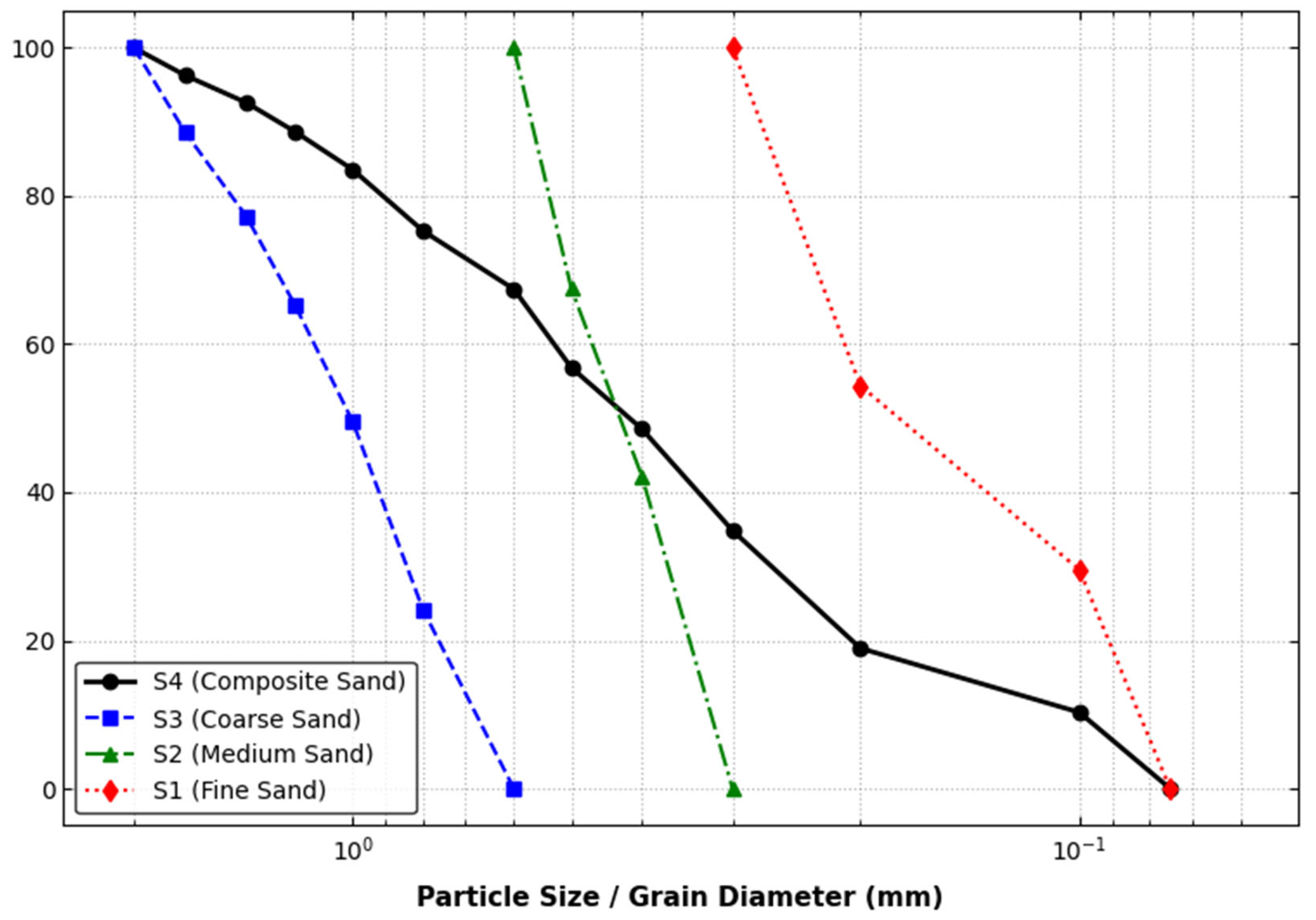
To systematically decouple the influence of the internal void architecture and particle size distribution on the emitted acoustic fingerprints, the baseline granular material was mechanically fractionated into discrete sub-bands, which were subsequently recombined to formulate four strictly defined soil typologies. Each typology was statistically defined by its characteristic diameter, D 30 , a parameter mathematically representing the effective sieve aperture dimension through which exactly 30% of the soil mass passes. It is usually taken as the characteristic diameter because this parameter is widely considered a reliable representative of the average particle diameter for these types of granular soils:
  • Fine Fraction ( S 1 ): Particle sizes spanning 0.075 to 0.3 mm (characteristic diameter, D 30 = 0.10 mm).
  • Medium Fraction ( S 2 ): Particle sizes spanning 0.3 to 0.6 mm (characteristic diameter, D 30 = 0.37 mm).
  • Coarse Fraction ( S 3 ): Particle sizes spanning 0.6 to 2.0 mm (characteristic diameter, D 30 = 0.85 mm).
  • Composite Mixture ( S 4 ): A well-graded, highly heterogeneous matrix reconstructing the original sand spectrum from 0.075 to 2.0 mm (characteristic diameter, D 30 = 0.27 mm).
Figure 1 represents the precise particle size distribution profiles of the four sand samples mentioned above.
To quantify the profound impact of interstitial fluid on the micro-mechanical friction coefficients, an exhaustive hydration matrix was designed. Each of the four soil typologies was meticulously prepared at five distinct moisture contents ( ω c ): 0% (representing the dry, high-friction state), 3%, 6%, 9%, and 12%.
A total of 24 distinct experimental samples were conceptualised and tested to feed the multivariate statistical model. To establish a stable, geometrically interlocked initial fabric and prevent unpredictable macroscopic collapse anomalies, the core 20 samples were subjected to mechanical vibration during their placement. Conversely, 4 additional non-vibrated samples (exclusively dry, ω c = 0%) were included to mathematically isolate the “initial fabric” variable. The complete characterisation of the initial statistical boundary conditions for the 24 discrete samples—including their specific gravity ( G s ), initial void ratio ( e 0 ), and initial dry density ( ρ d , 0 )—is detailed in Table 1.
Reproducibility was strictly ensured by adhering to a highly standardised dry-hydration and compaction protocol. This guaranteed that for any target boundary condition, the execution variance (human or procedural error) is minimised, ensuring that the changes in acoustic emission signatures are exclusively driven by the intended physical variables.

2.2. Stress Regimes and Macroscopic Geotechnical Monitoring

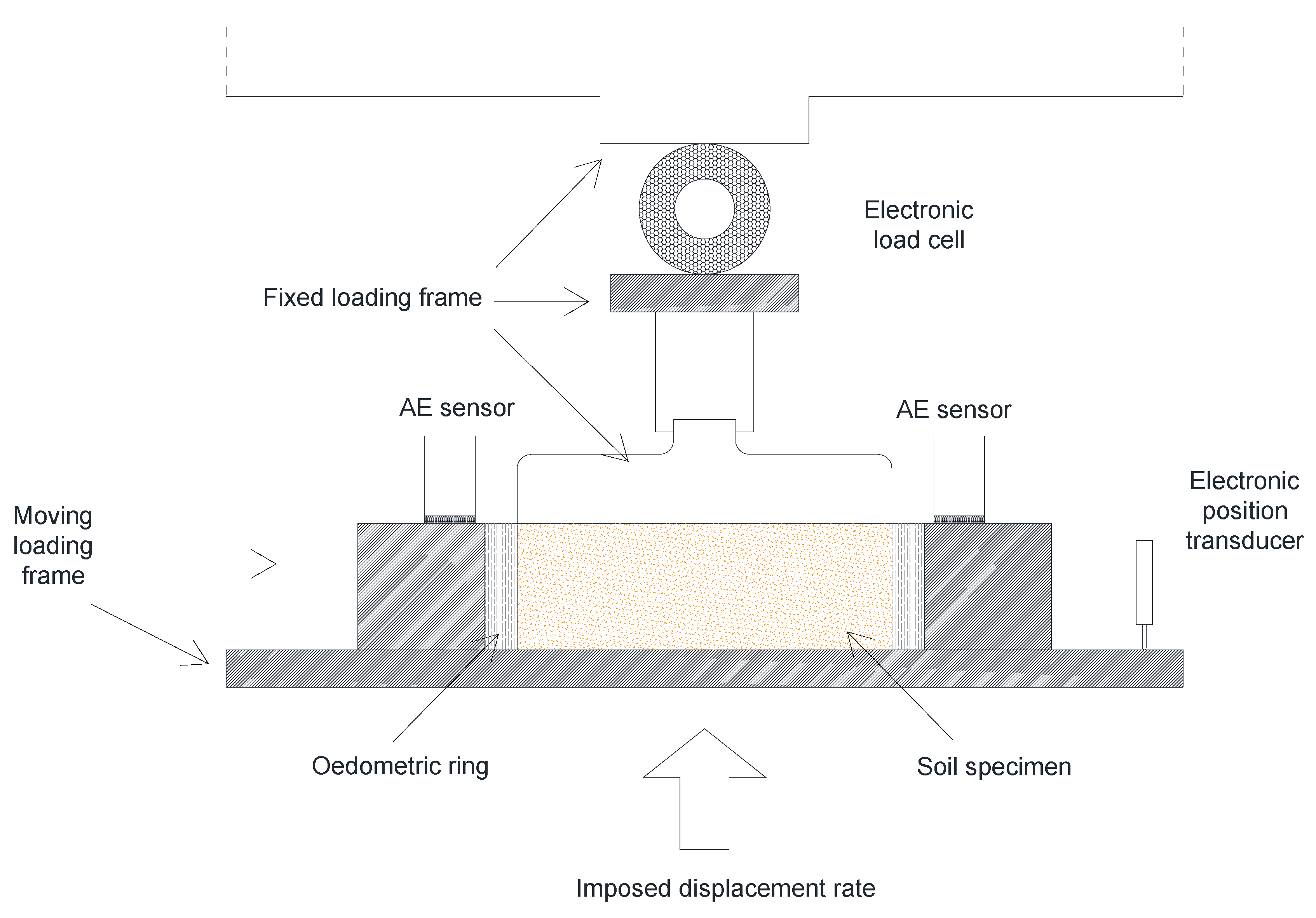
The samples were structurally confined within a highly rigid metallic oedometric cell, mathematically defining a constant volumetric perimeter of V 0 = 39.27 cm3 (internal diameter ϕ i n t = 50 mm; initial specimen height H 0 = 20 mm). The external boundary energy was applied via a high-precision, automated 50 kN electro-mechanical press. To maintain dynamic equilibrium and ensure that the statistical noise generated corresponded purely to stable soil rearrangement rather than impact shock, the uniaxial strain was driven continuously at a strictly controlled rate of 1 mm/min. Given the small sample size (initial height of 20 mm), the total duration of each test was inherently restricted to a maximum of 3–4 min. Within this brief timeframe, the sand matrix achieved high vertical strain levels (up to 20%), driving the applied stress to the upper experimental limit, which, for equipment safety, was set at 5000 kPa. Because the instrumentation is restricted to a single, rapid primary compression path, time-dependent rheological phenomena—such as secondary creep or stress relaxation—are physically negligible. Figure 2 shows the schematic setup of the experimental apparatus, illustrating the precise location of the geotechnical monitoring instrumentation along with the sensors of the acoustic emissions acquisition system.
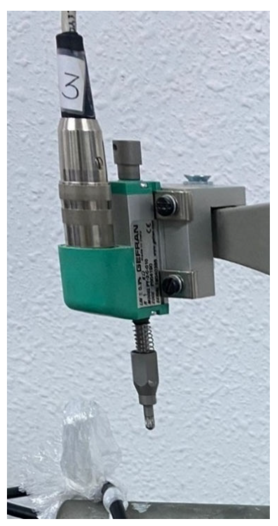
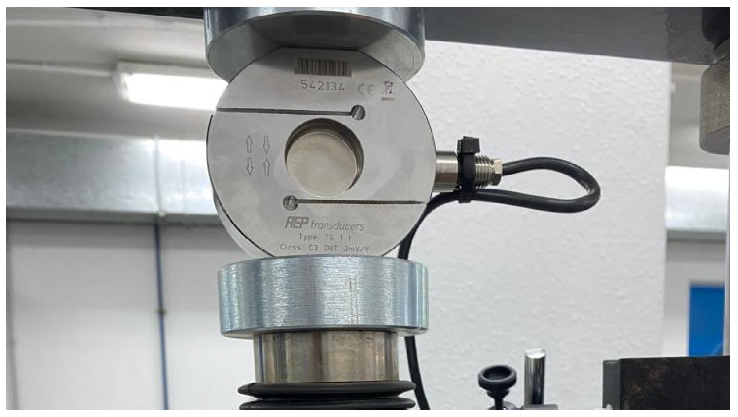
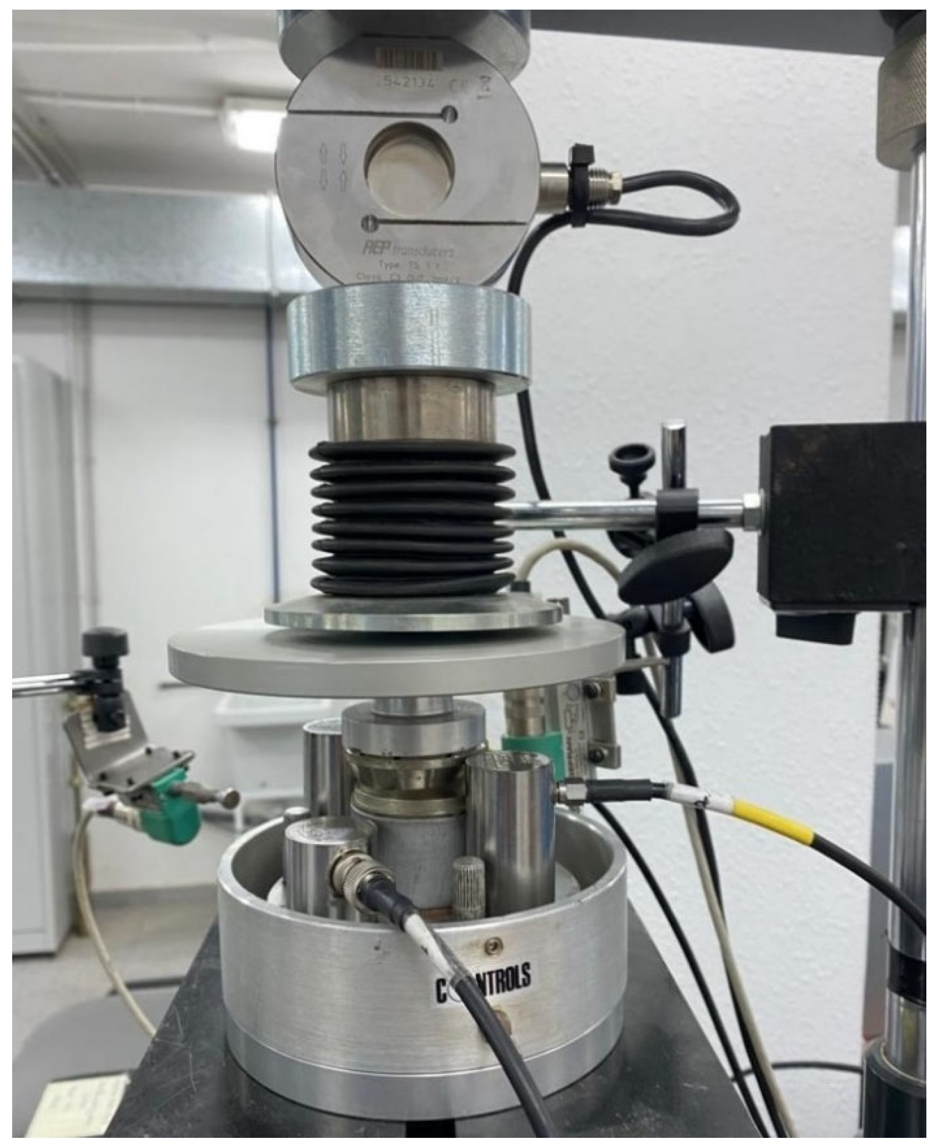
The temporal evolution of the system was captured using highly sensitive digital transducers. The absolute vertical settlement was dynamically mapped by a Gefran PY-2-C-010 electronic position transducer (1 µm resolution, Figure 3), while the resistive boundary force was quantified by an AEP Transducers TS 1t C3 electronic load cell (0.1 N resolution, Figure 4). Both digital streams were synchronised at a 1 Hz sampling frequency utilising a Matest Cyber Plus Evolution data acquisition hub.
To execute discrete statistical analysis, the continuous compression timeline was partitioned into nine specific loading stages (ls). Following a fundamental pre-load stage (12.5 kPa) designed to seat the instrumentation and eliminate initial macroscopic voids, the vertical effective stress ( σ v ) was escalated through the specific bounds detailed in Table 2.

2.3. Micro-Mechanical Acoustic Emission (AE) Acquisition Framework

In recent years, standardisation in AE terminology [38] and its deployment in diverse physical contexts—such as deep rock stability evaluation [39,40,41,42], structural wire drawing monitoring [43], damage evolution in composite beams [44], and fracture monitoring in concrete matrices [12]—have firmly established AET as a critical tool for mapping internal stress dynamics.
In this research, to bridge the macroscopic boundary conditions with the invisible micro-mechanical phenomena, a dual-layer, multi-channel acoustic array was engineered. The array was strategically coupled directly to the rigid metallic baseplate supporting the oedometric ring. Acoustic emission tracking was achieved using four passive resonant piezoelectric sensors positioned in a highly symmetric orthogonal quadrant layout (spaced at 90° intervals), Figure 5.
  • Two Vallen VS30-SIC-46 dB Sensors (spaced at 180° intervals): Operating optimally within the 25–100 kHz low-frequency band. These sensors act as the primary receptors for the prolonged, lower-energy acoustic signatures originating from spatial rearrangement and grain-boundary sliding friction.
  • Two Vallen VS900-RIC Sensors (spaced at 180° intervals): Operating as broadband receptors (100–900 kHz). These devices are specifically tuned to detect the highly transient, sharp acoustic impulses released during high-stress asperity abrasion and particle micro-cracking.
The purpose of this spatial arrangement is twofold: to provide symmetric wave-capture redundancy and to mathematically average out spatial signal attenuation inside the metallic testing cell. To eliminate boundary reflection and air-gap wave scattering, a high-viscosity, chemically stable lithium grease was applied to the active faces of the sensors and the structural connection of the metal base plate with the oedometric ring. The sensors, embedded in the support plate, maintained a critical travel distance of less than 3 cm from the compressed sand particles, effectively circumventing the severe signal attenuation and dispersion typical of wave transmission through unsaturated granular porous media.
The raw analogue signals were transmitted to a Vallen AMSY-6 data acquisition unit. Based on rigorous environmental background testing, a strict amplitude threshold of 40 dB was established. This threshold acted as the primary analogue filter, successfully isolating the genuine micro-mechanical events from the parasitic ambient noise and the mechanical hum of the actuator.

2.4. Mathematical Formulation, Data Processing, and Multivariate Statistical Architecture

The analytical core of this study relies on the precise temporal synchronisation of the macroscopic geotechnical data streams with the microscopic AE hits, establishing a rigorous mathematical framework suitable for predictive modelling. Utilising custom algorithms developed in Python 3.10.5 (leveraging pandas, numpy, and scipy libraries), millions of discrete AE hits were parsed, filtered, and aggregated per discrete loading stage.

2.4.1. Mathematical Definition of the Feature Vectors

To rigorously capture the historical evolution of the system’s statistical complexity, it was mathematically imperative to define multiple formulations for the extracted variables. Granular deformation under compression is a highly path-dependent thermodynamic process; therefore, evaluating a parameter solely at an isolated instant omits crucial information regarding cumulative damage, structural memory, and previous spatial rearrangement. To accurately model this complexity, specific macroscopic properties and microscopic AE parameters were mathematically formulated using three distinct deformation criteria, denoted by their respective subscripts:
  • Current loading stage ( P l s ): The arithmetic mean of the parameter (P) calculated exclusively for the hits detected within a specific loading stage.
  • Average up to the loading step ( P a , u , l s ): The arithmetic mean of all hits recorded from the beginning of the test up to the current stage, capturing the system’s global loading history.
  • Weighted average up to the loading step ( P w a , u , l s ): The weighted average of all hits recorded from the beginning of the test up to the current stage (capturing the system’s global loading history), taking into account the proportion of hits in each interval.
The selection of the three proposed temporal aggregation frameworks—namely stage-specific, history average, and weighted history average metrics—is explicitly governed by the micromechanical nature of acoustic emission (AE) generation. Granular media subjected to compression exhibit pronounced path dependency and structural memory (e.g., damage accumulation and the Kaiser effect). Non-parametric point-metrics, such as medians or percentiles, are structurally insensitive to the continuous accumulation of elastic energy dissipation. Therefore, although the three proposed historical aggregations exhibit mathematical cross-correlation, they are preserved within this multivariate analysis because they represent distinct physical dimensions of the soil’s stress–strain history, which is vital for maintaining the generalisability of the predictive framework.
The comprehensive set of macroscopic geotechnical state variables incorporated into the analytical model is systematically summarised in Table 3. This selection of thirteen parameters provides a high-resolution map of the soil’s mechanical evolution. To ensure consistency with established predictive frameworks, the mathematical formulation of these variables follows the methodology previously validated by García-Ros et al. [35]. This includes the derivation of critical state parameters—such as the coefficient of compressibility ( a v ) and the compression index ( c c )—which defines the material’s evolving deformability as a function of the effective vertical stress ( σ v ) and void ratio ( e ):
c c , l s = e f , l s e o , l s log 10 ( σ f , l s σ o , l s )
a v , l s = e f , l s e o , l s σ f , l s σ o , l s
where the subscripts o , l s and f , l s designate the absolute initial and final boundary points of the respective loading stage. Notably, due to the profound path-dependent nature of soil deformability, the compression index was explicitly evaluated using the three aforementioned temporal formulations ( c c , l s , c c , a , u , l s and c c , w a , u , l s ) to precisely model its evolutionary trend.
A total of 48 acoustic emission descriptors were integrated into the multivariate framework, as detailed in Table 4, following the mathematical formulation of Castro et al. and García-Ros et al. [34,35]. These descriptors are derived from the AE transient waveforms (a total of 16 acoustic variables comprising classic parametric features such as counts, energy, amplitude, duration, frequency, rise time, etc.) and their aggregations across the three proposed temporal domains: stage-specific (ls), history average (a,u,ls), and weighted history average (wa,u,ls).
The acoustic feature space incorporates fundamental metrics such as the hits number ( N H i t ), peak amplitude ( A ), true linear amplitude ( A v , l s ), duration ( D ), average frequency ( F ), counts ( C N T S ), rise time ( R T ), and energy ( E ), alongside other advanced descriptors that were included to standardise waveform characterisation: signal strength and peak signal strength ( S s ;   S s , p ), RA ( R A ), earliness, transitoriness and early transitoriness ( e a r l ; T r ; e T r ) [34], and cumulative acoustic energy and signal strength from the start of the test ( E c u m ; S s , c u m ).
Furthermore, adapting the classical macro-seismological principles of Gutenberg and Richter [45] and Benioff [46] to the micro-mechanical scale [47,48], the statistical descriptors b-value and r-value ( b ; r ) were computed to map the evolving severity of the structural damage. For this study, the Gutenberg–Richter b-value was determined by mathematically extracting the negative slope of the linear regression relating the decimal logarithm of the cumulative number of hits exceeding a specific amplitude threshold to the decimal logarithm of that amplitude.
The raw geotechnical and acoustic data corresponding to the 24 tested samples (20 vibrated and 4 non-vibrated, Table 1), utilised for the correlation and regression analyses in this study, are provided in the Supplementary Materials. This ensures full transparency and reproducibility of the statistical framework presented.

2.4.2. Statistical Correlation and Empirical Regression Modelling

Once the synchronised feature vectors were assembled, they were dynamically partitioned into the five designated analytical blocks outlined in Section 1. To rigorously quantify the strength and linear directionality between the acoustic predictors (independent variables, x) and the target macroscopic geotechnical states (dependent variables, y), Pearson’s correlation coefficient p was computed matrix-wide:
p x y = s x y s x s y
where s x y is the covariance between the variables x and y, while s x and s y are the respective standard deviations. This statistical coefficient, rigidly bounded within [−1, +1], functioned as the primary metric to identify optimal predictive relationships and enhance the resolution of the geomechanical state inference.
Following the isolation of high-correlation pairs, empirical predictive models were mathematically constructed. Leveraging the Ordinary Least Squares (OLS) algorithm, polynomial regression functions of orders 1, 2, and 3 were fitted to the datasets. The final predictive model for each variable pair was selected by mathematically maximising the coefficient of determination (R2). This multi-order approach ensures that the highly non-linear, asymptotic behaviour of the granular matrix under extreme compression is accurately captured and reliably inferred from the passive acoustic data. In this context, while the preliminary Pearson correlation coefficient ( p ) was deployed as an initial, computationally straightforward, screening filter to evaluate the strength of the dependencies, it is fundamentally restricted to first-order linear relationships and may under-represent non-monotonic trends; hence, these underlying physical non-linearities were systematically recovered and parametrically mapped through the subsequent polynomial architectures.
To ensure that the empirical regression coefficients remain structurally stable and immune to potential sample size constraints across the sand cohorts ( S 1 to S 4 ), a comparative sensitivity and parameter-stability validation was performed. Given the deterministic nature of the boundary conditions in these 24 highly controlled laboratory environments with equal sample sizes, the intrinsic variance remains minimal. The sensitivity analysis confirmed that the model topographies are numerically resilient; the predictive divergence observed between uniform fractions ( S 1 , S 2 , S 3 ) and the well-graded compound matrix ( S 4 ) represents genuine micromechanical transitions—such as localised grain contact density and spatial rearrangement—rather than mathematical artefacts or statistical bias induced by sample size allocation.

3. Results and Discussion

The experimental and statistical framework described in the previous section yielded a high-dimensional dataset that captures the emergent behaviour of granular sands under compressive stress. The following analysis is structured into five analytical blocks, each designed to isolate specific geomechanical and structural constraints to decode the underlying complexity of the acoustic signatures. First, a global baseline is established through Generalised Correlations (Section 3.1), followed by a systematic evaluation of the influence of Soil Typology (Section 3.2) and the lubricating effects of moisture c ontent (Section 3.3). Furthermore, the transition between different stress Regimes (Section 3.4) is examined to identify the shift in dominant micromechanical processes. Finally, the Influence of Initial Fabric (Section 3.5) is assessed by contrasting different compaction states. Collectively, these sections provide a robust mathematical architecture for the indirect inference of macroscopic state variables from stochastic acoustic events.

3.1. Block 1: General Statistical Baseline (Vibrated Soils)

To establish a fundamental statistical baseline, the initial analysis integrated the complete matrix of the twenty mechanically vibrated samples (encompassing all four soil typologies, S 1 through S 4 , across all five moisture contents, from ω c = 0% to 12%). The multivariate analysis of this global dataset demonstrated that every single monitored geotechnical variable exhibited at least a moderate degree of correlation ( | p | ≥ 0.43) with one or more acoustic parameters (Table 5). Furthermore, a significant majority of the regression functions yielded high correlation degrees ( | p | ≥ 0.60); Table 5.
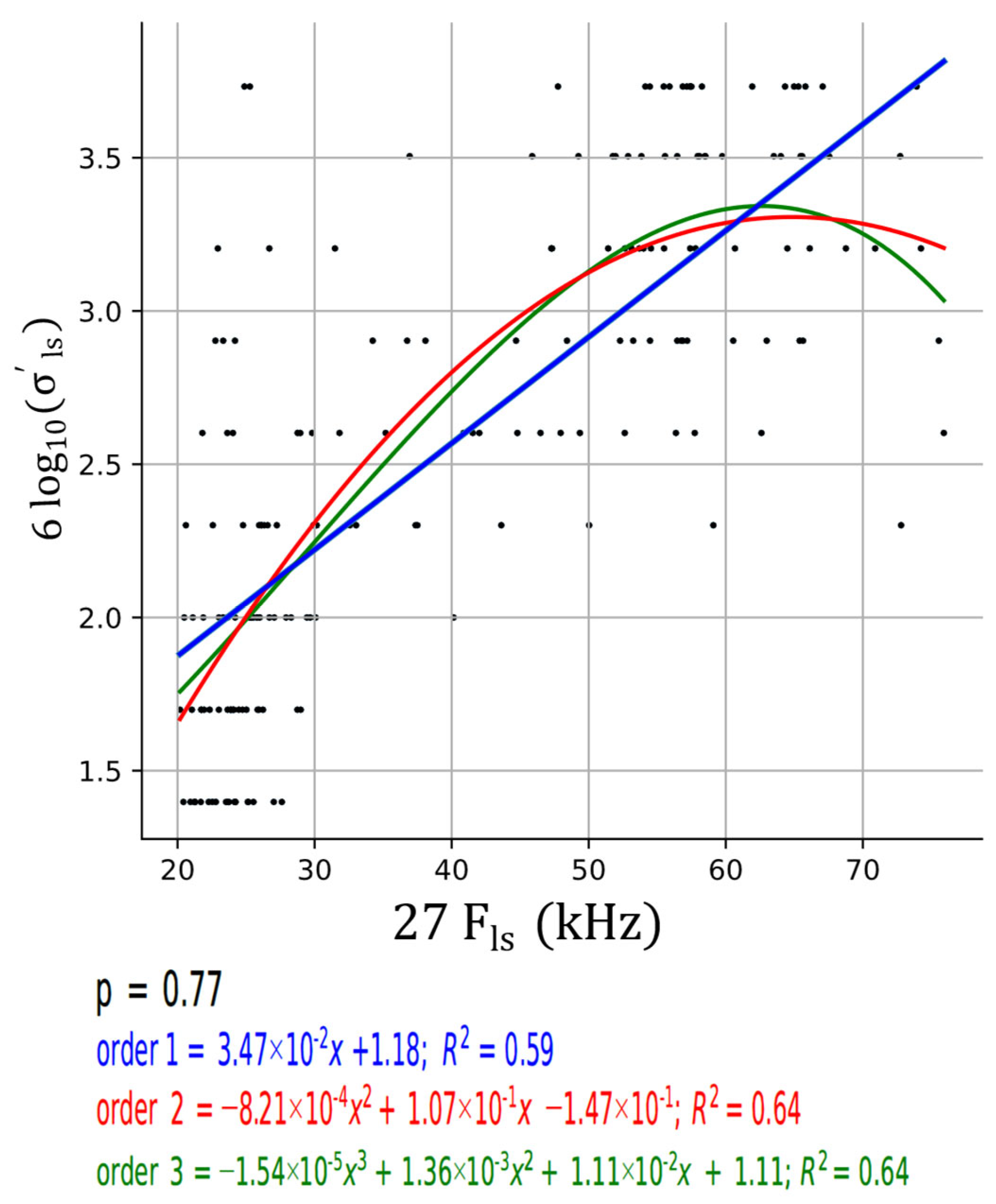
Most notably, within this general baseline, the base-10 logarithm of the effective stress ( log 10 ( σ l s ) , ID = 6) emerged as the variable with the strongest predictive potential, showing a robust correlation ( p = 0.77) with the average frequency of the loading stage ( F l s , ID = 27); Table 5 and Figure 6. These results confirmed the overarching hypothesis: it is entirely feasible to infer macroscopic geotechnical properties directly from the acoustic signatures, provided the soils are adequately compacted.
Regarding the predictive architecture, the selection of the polynomial degree is dictated by the inherent complexity of the geomechanical–acoustic coupling. First-degree polynomial regression models prove ideal for initial exploratory phases and for variables exhibiting a direct proportional relationship or strong monotonicity, such as the characteristic grain diameter ( ϕ s ), moisture content ( ω c ), base-10 logarithm of the effective stress ( log 10 ( σ v ) ), or basic acoustic metrics like the hits number ( N H i t ), amplitude ( A ), and counts ( C N T S ). Conversely, higher-order refinements are achieved through second-degree polynomials when the data manifest non-linear curvature, or third-degree polynomials to accurately model “S-shaped” transitions and specific inflexion points. This hierarchical modelling approach ensures a robust balance between capturing the intricate structures of the granular system and minimising potential stochastic noise.

3.2. Block 2: The Impact of Granulometry (Soil Typology)

To systematically evaluate the profound influence of particle size distribution on the emitted acoustic signatures, this analytical block isolates the four distinct soil typologies ( S 1 through S 4 ) and subsequently confronts them mathematically. All evaluated samples within this block were strictly limited to the twenty mechanically vibrated matrices to eliminate the confounding variables associated with a loose initial fabric.

3.2.1. Analysis of Isolated Soil Fractions

When analysed independently, all four soil typologies demonstrated a remarkable capacity to predict geotechnical variables, with every variable exhibiting at least a moderate correlation ( | p | ≥ 0.46) with the acoustic parameters.
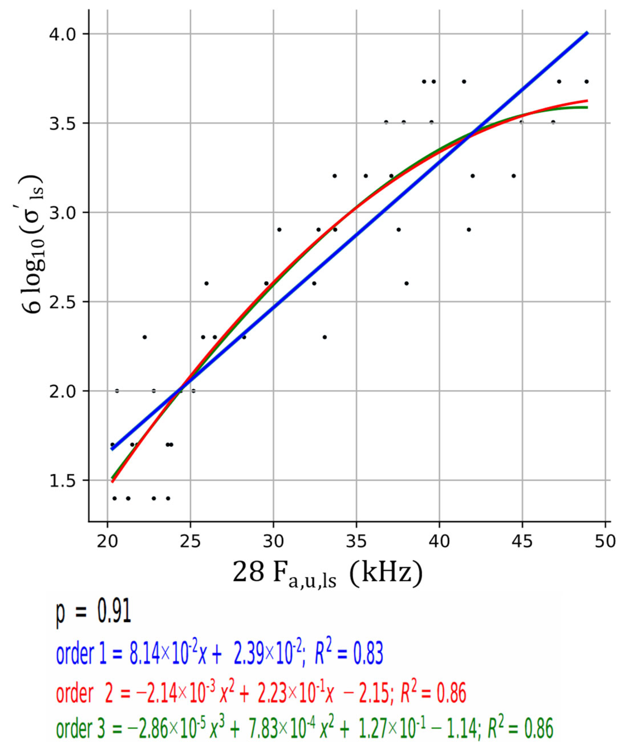
  • The Intermediate Fraction ( S 2 ): This specific gradation (0.3–0.6 mm) yielded the highest predictive accuracy across the entire experimental programme. For S 2 , every single monitored geotechnical variable achieved high ( | p | ≥ 0.65) to very high ( | p | ≥ 0.80) correlation degrees; Table 6. The strongest correlation overall was observed within this fraction, reaching an exceptional p = 0.91 between the base-10 logarithm of the effective stress ( log 10 ( σ l s ) ) and the average frequency up to the loading stage ( F a , u , l s , ID = 28); Table 6 and Figure 7.
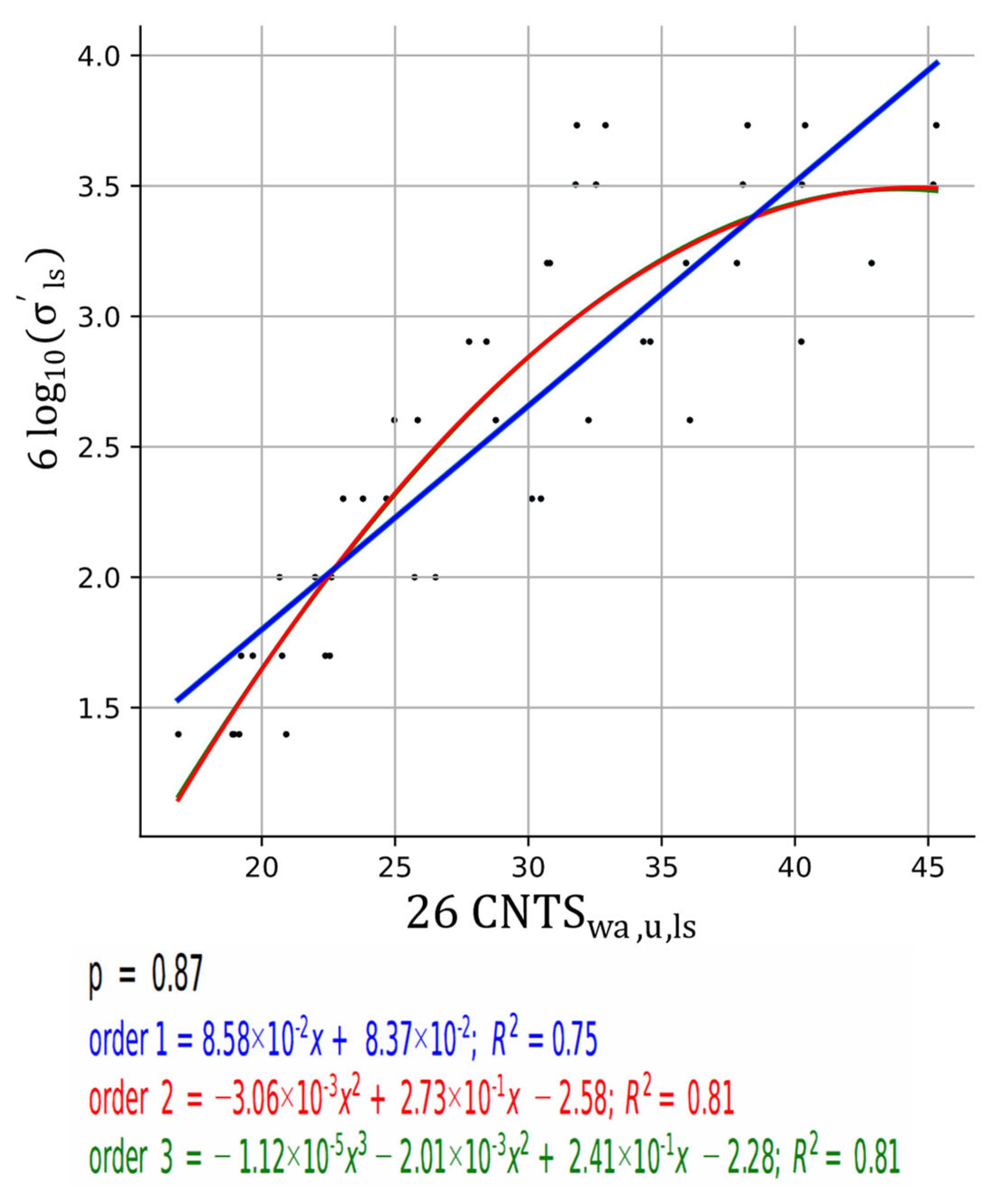
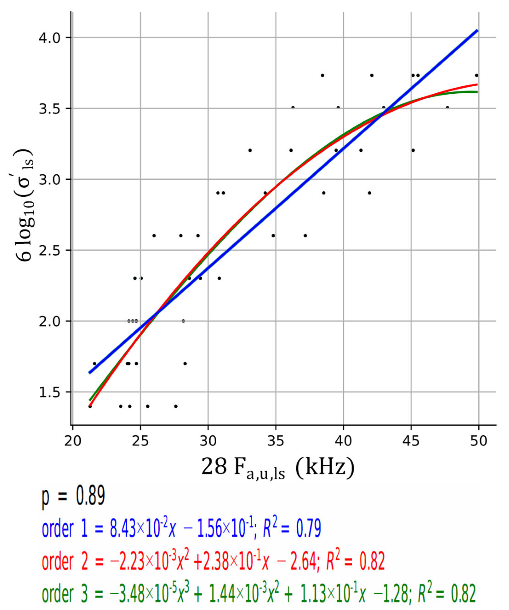
  • The Coarse Fraction ( S 3 ) and Composite Mixture ( S 4 ): Both of these typologies also exhibited outstanding predictive capabilities; Table 7 and Table 8. For these materials, the effective stress ( log 10 ( σ l s ) ) remained the most reliably inferred variable, correlating robustly with the cumulative acoustic counts ( C N T S w a , u , l s , ID = 26) in S 3 ( p = 0.87; Table 7 and Figure 8) and the average frequency ( F a , u , l s ) in S 4 ( p = 0.89; Table 8 and Figure 9). This solidifies the fundamental link between macroscopic stress increments and high-frequency, high-count acoustic phenomena driven by severe asperity abrasion.
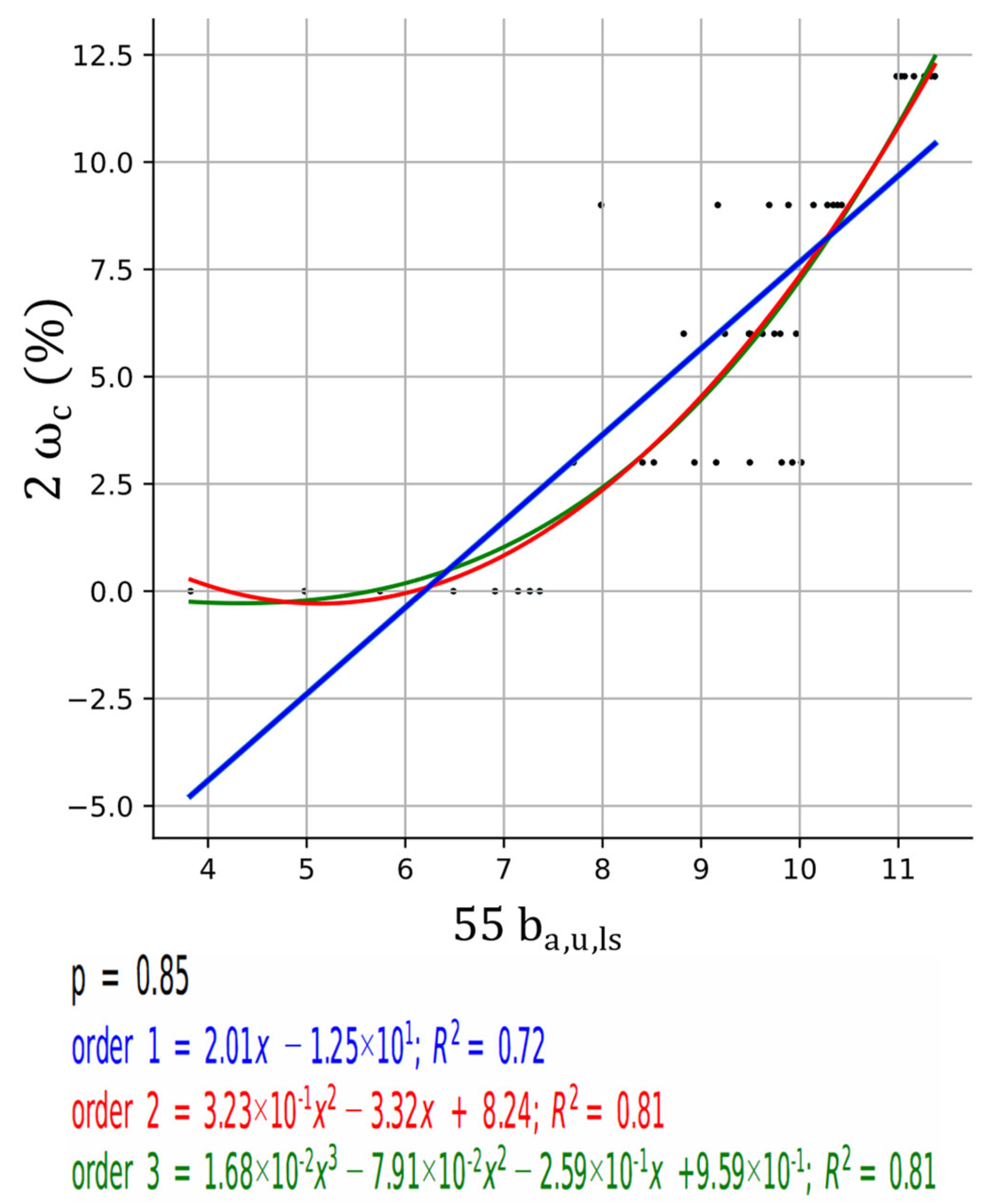
  • The Fine Fraction ( S 1 ): While S 1 (0.075–0.3 mm) presented slightly lower overall correlation degrees compared to the coarser fractions, it revealed a highly specific and physically significant acoustic behaviour. For this fine sand, the moisture content ( ω c , ID = 2) emerged as the most predictable variable, correlating remarkably well ( p = 0.85) with the average b-value up to the loading stage ( b a , u , l s , ID = 55); Table 9 and Figure 10. This statistical relationship phenomenologically corroborates the lubricating effect of water: in fine-grained matrices, which possess an exponentially higher number of contact points per unit volume, interstitial fluid facilitates smooth, low-energy grain sliding. This lubrication drastically reduces the emission of high-amplitude transient hits, thereby driving the b-value up.

3.2.2. Confrontation of Disparate Granulometries

To rigorously assess the mathematical robustness of these predictive models across heterogeneous matrices, a series of statistical “confrontations” was executed. The discrete, uniform fractions were directly contrasted against the well-graded original sand ( S 1 vs. S 4 , S 2 vs. S 4 , and S 3 vs. S 4 ), alongside a holistic confrontation of the three uniform fractions simultaneously ( S 1 , S 2 , and S 3 ).
The integration of these disparate granulometries into combined datasets successfully demonstrated that acoustic signatures can mathematically distinguish between uniform and well-graded physical states. In uniformly graded soils ( S 1 , S 2 , S 3 ), the macroscopic boundary load is distributed across similarly sized contact points, promoting highly specific, concentrated friction and fracture events. In stark contrast, the well-graded composite ( S 4 ) possesses a heterogeneous void distribution where smaller grains actively cushion the larger particles. This “cushioning” effect alters the internal stress transmission networks, fundamentally shifting the dominant acoustic frequencies and the distribution of acoustic energy.
Consequently, the confrontation models establish a critical premise for geo-acoustic monitoring: while predicting the general state of a highly heterogeneous soil deposit is entirely feasible using global parameters, the highest degree of mathematical precision and predictive accuracy requires regression functions tailored explicitly to the characteristic diameter ( ϕ s ) of the dominant soil fraction.
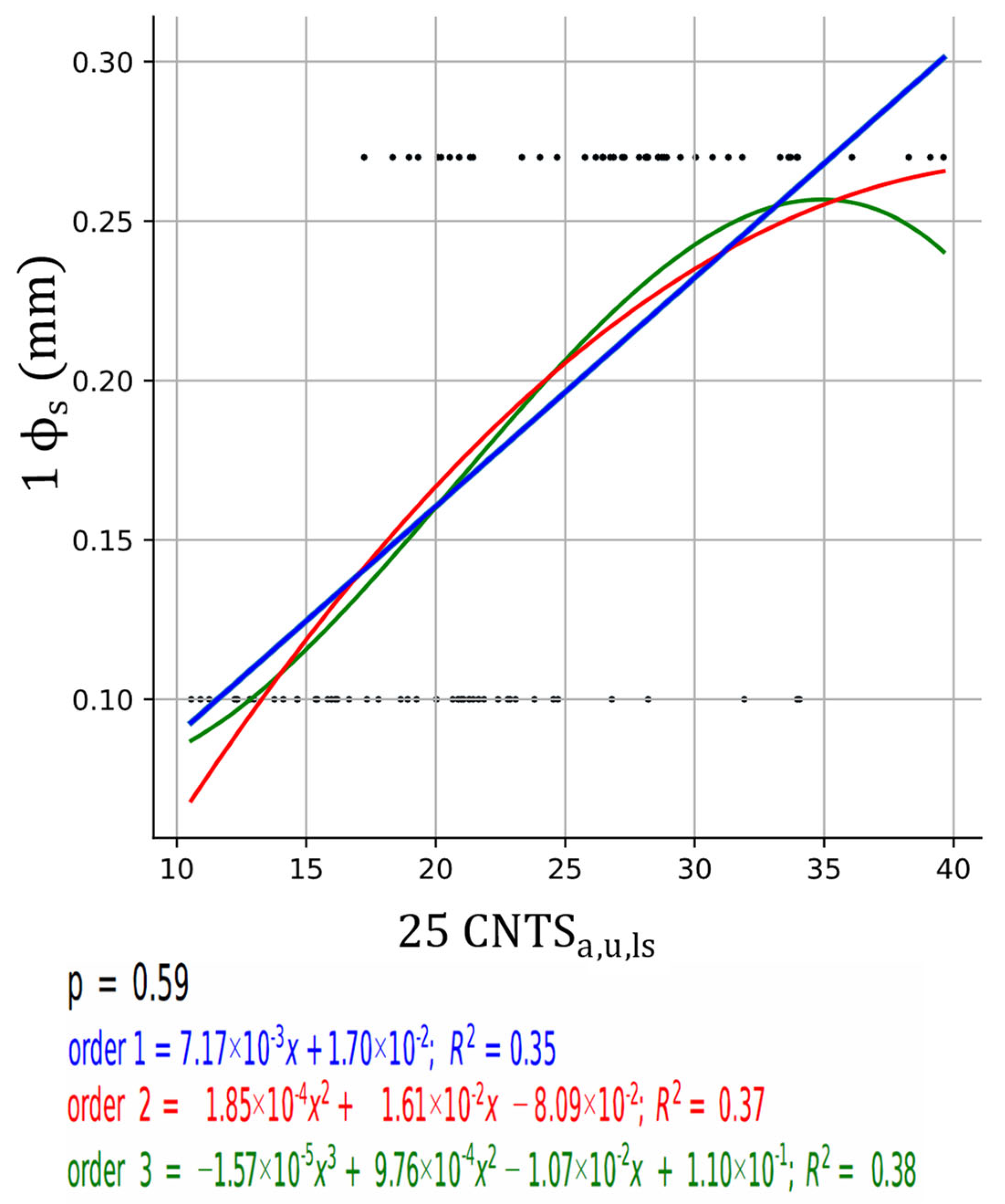
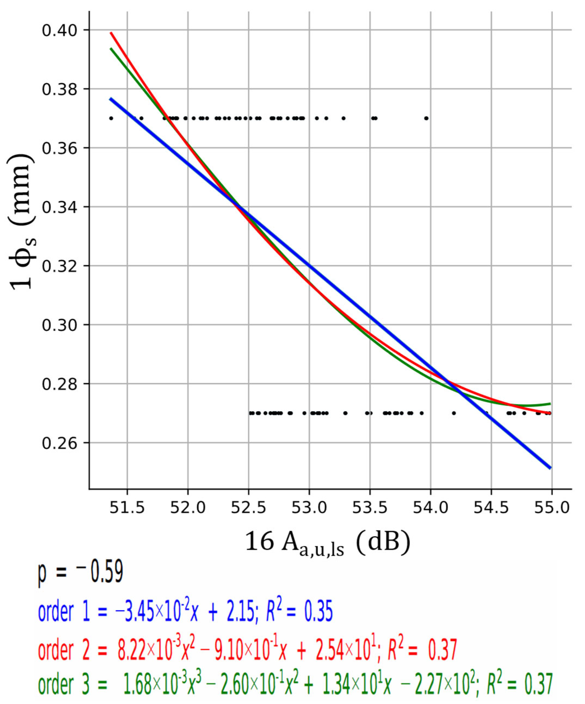
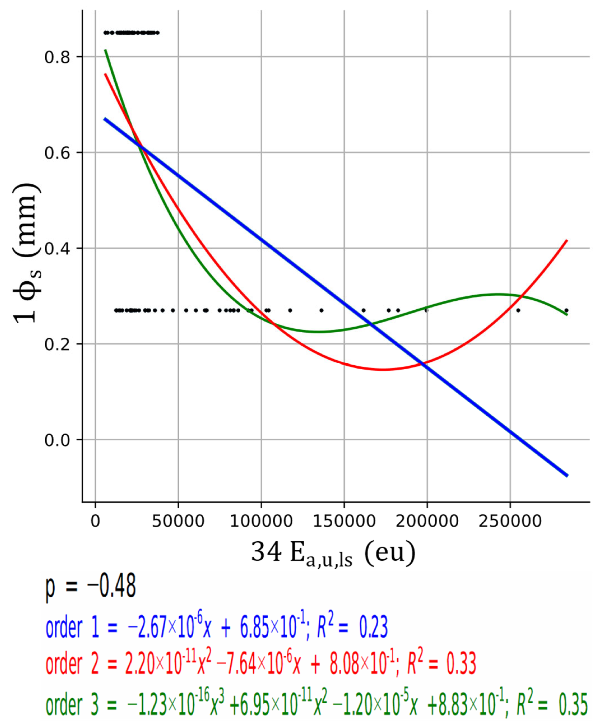
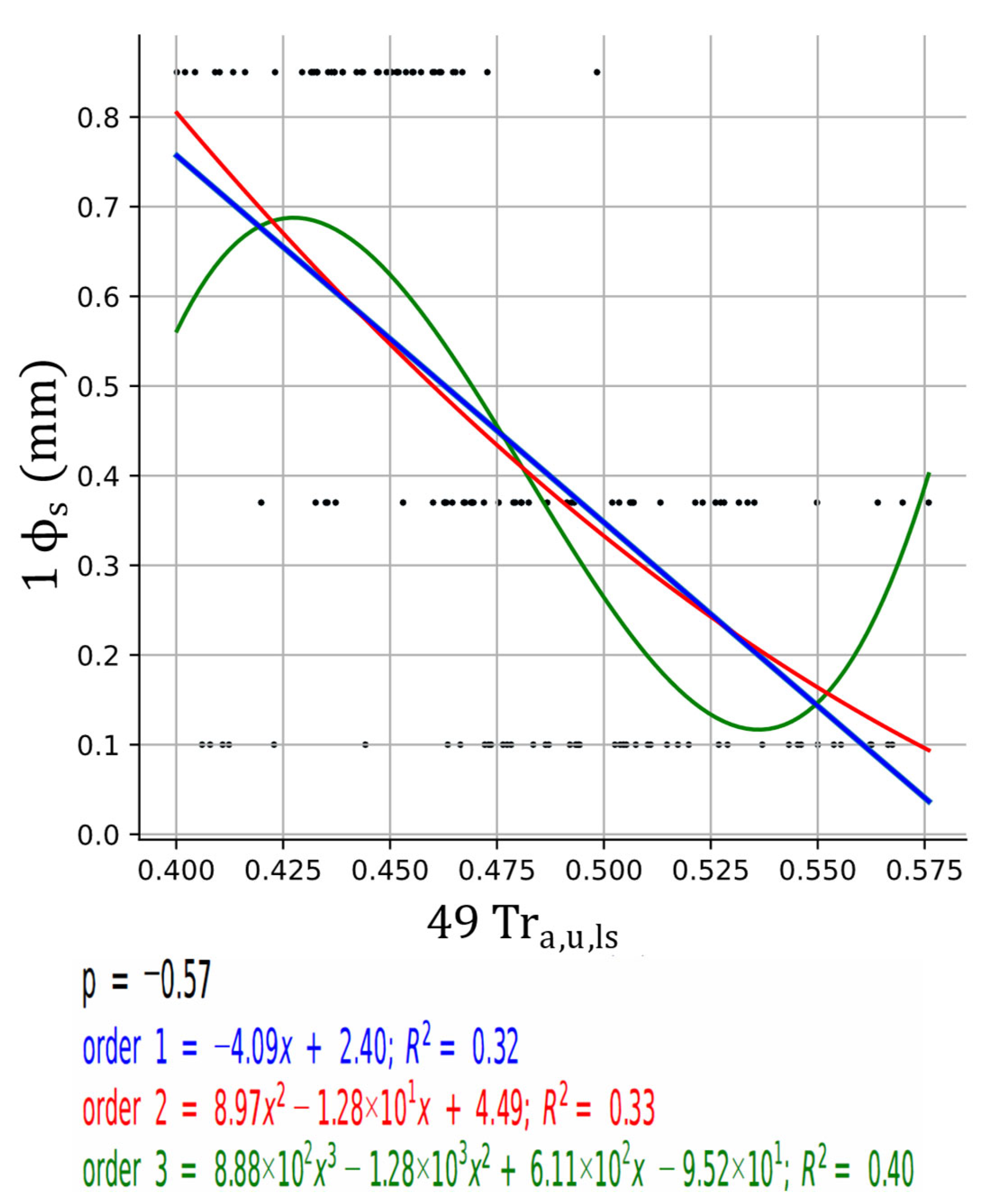
In this context, Figure 11, Figure 12, Figure 13 and Figure 14 illustrate the regression functions and trend lines for the most significant correlations identified between the characteristic grain diameter ( ϕ s ) and the diverse set of acoustic emission descriptors. These predictive frameworks are established for the complete suite of mechanically vibrated specimens across distinct granulometric combinations: soils S 1 - S 4 (Figure 11), S 2 - S 4 (Figure 12), S 3 - S 4 (Figure 13), and the triple-fraction comparison S 1 - S 2 - S 3 (Figure 14).
Within these analytical domains, Pearson’s correlation coefficients yielded moderate values, ranging between 0.5 and 0.6. Such statistical significance confirms that these correlations can be valid for discriminating between uniform granular textures and well-graded soil matrices (Figure 11, Figure 12 and Figure 13), or between uniform distributions but of different grain sizes (Figure 14).
Thus, in the comparisons of the composite mixture ( S 4 ) with each of the three uniform samples, we observe that the fine fraction S 1 presents acoustic signatures with a lower C N T S variable (Figure 11); this means that the fine fractions will present acoustic signatures of shorter duration. For its part, the intermediate fraction S 2 shows lower amplitudes, that is, lower energy, with this being the same effect observed for the coarse fraction S 3 (Figure 12 and Figure 13).
On the other hand, when we compare the three uniform granulometries (Figure 14), we observe how, as the diameter increases, the T r variable decreases, which, in the way that this variable is defined [35], translates into more transient (less stationary) acoustic waves.

3.3. Block 3: The Effects of Interstitial Fluid (Moisture Content)

To rigorously quantify the lubricating effects of interstitial fluid on the generation of acoustic emissions, this analytical block evaluates the soil matrices across a strict spectrum of predetermined moisture contents ( ω c = 0%, 3%, 6%, 9%, and 12%). To ensure a balanced and noise-free statistical analysis, the dataset was strictly restricted to mechanically vibrated samples. The evaluation was conducted across two parallel tracks: first, confronting exclusively the three uniform discrete fractions ( S 1 , S 2 , S 3 ), and second, expanding the confrontation to include the well-graded composite original mixture ( S 1 , S 2 , S 3 , S 4 ). Given the high degree of similarity observed in both the acoustic and geotechnical datasets across these two tracks—particularly regarding the three initial soil typologies—the resulting correlations proved to be remarkably consistent. Consequently, for the sake of analytical conciseness, this section will focus exclusively on the comparative results obtained from the discrete fractions ( S 1 , S 2 , S 3 ).

3.3.1. Global Predictive Capacity Across Hydration States

The multivariate analysis demonstrated that the introduction of interstitial fluid does not diminish the predictive power of the acoustic emission technique. Across all evaluated moisture contents and both confrontation tracks, every monitored geotechnical variable maintained at least a high degree of correlation ( | p | ≥ 0.61) with specific acoustic parameters. This confirms that highly accurate empirical regression functions can be established to infer the soil state, provided the algorithm accounts for the specific in situ hydration level.

3.3.2. The Extreme Moisture Phenomenon: Stress-Driven Acoustics

A critical phenomenological pattern emerged when analysing the extremes of the hydration spectrum. For strictly dry soils ( ω c = 0%) and those nearing the critical saturation limit prior to water expulsion during compression ( ω c = 9% and 12%), the geotechnical variable that exhibited the absolute highest correlation degrees was the logarithmic effective stress ( log 10 ( σ l s ) ).
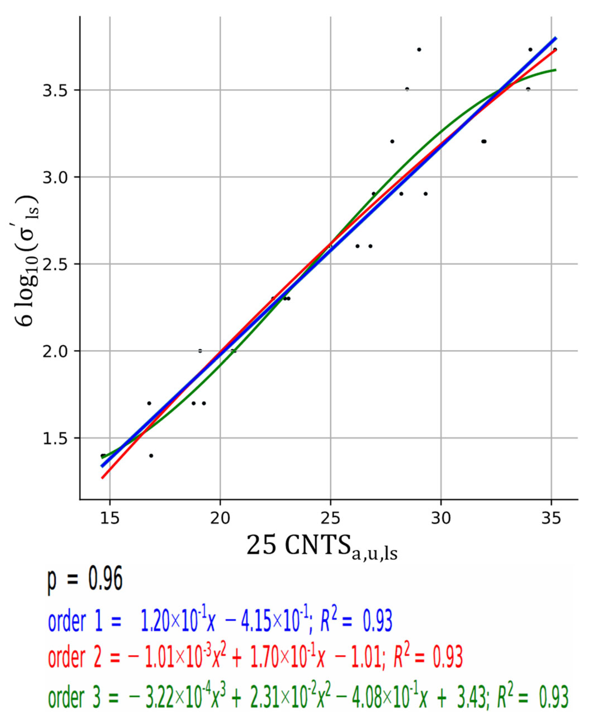
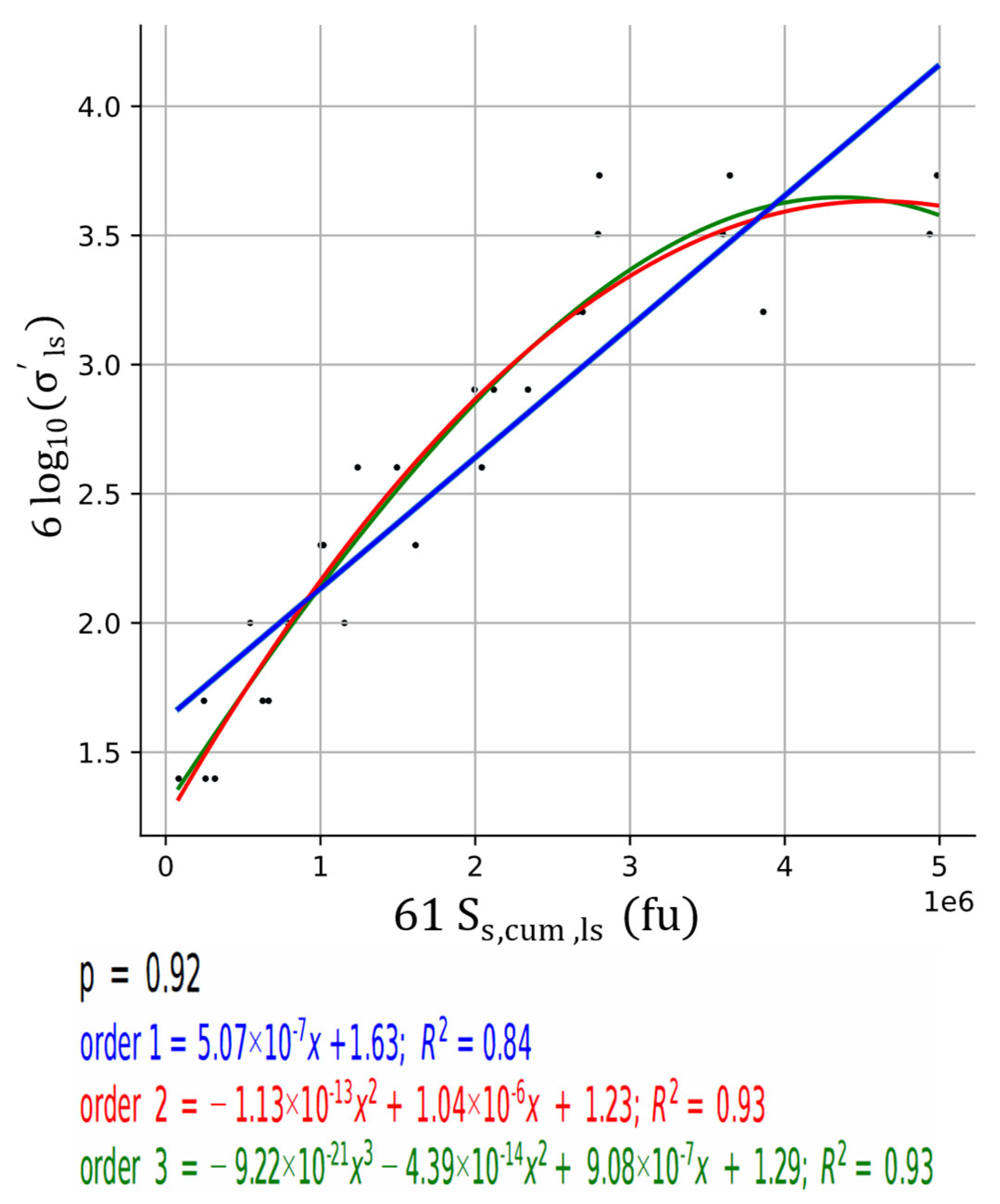
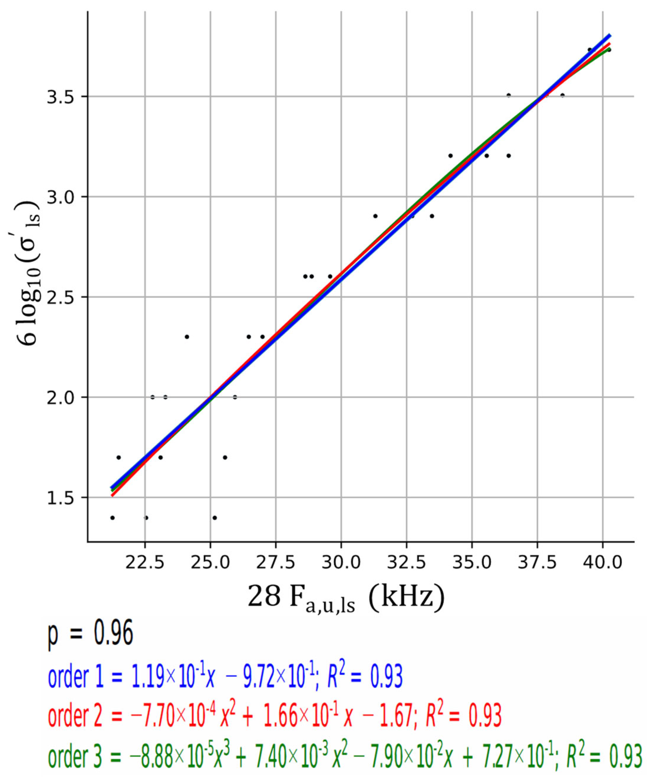
At these boundary states, the acoustic parameters that best predicted the applied stress were the cumulative counts ( C N T S a , u , l s , ID = 25), for ω c = 0%, Figure 15, the cumulative signal strength ( S s , c u m , l s , ID = 61), for ω c = 9%, Figure 16, and the average frequency ( F a , u , l s , ID = 28), for ω c = 12%, Figure 17, with values of | p | ≥ 0.92. Physically, this indicates that in the absence of moisture, or when the void spaces are nearly saturated, the acoustic energy and the spectral frequency are predominantly governed by the raw macroscopic load increments and the resulting severe inter-granular friction rather than by gradual soil yielding.

3.3.3. The Intermediate Moisture Phenomenon: Deformability and Lubrication

In stark contrast, a fundamental shift in acoustic behaviour was observed at intermediate moisture levels ( ω c = 3% and 6%). For these hydration states, the dominant, most predictable geotechnical variable shifted away from the effective stress towards the compression index ( c c ), specifically its weighted and arithmetic averages ( c c , w a , u , l s , ID = 11, and c c , a , u , l s , ID = 10).
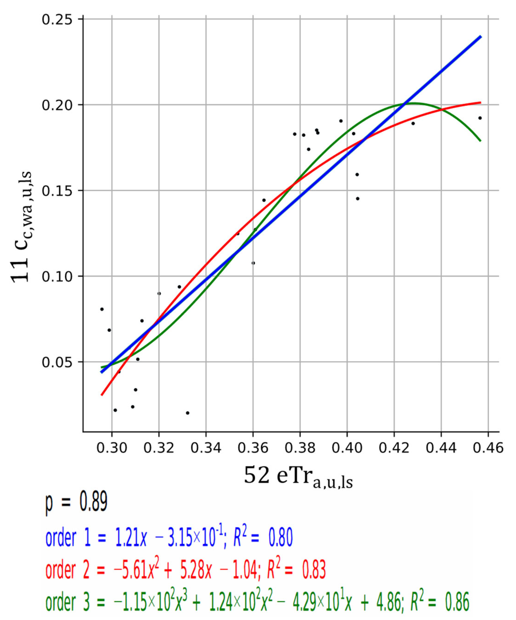
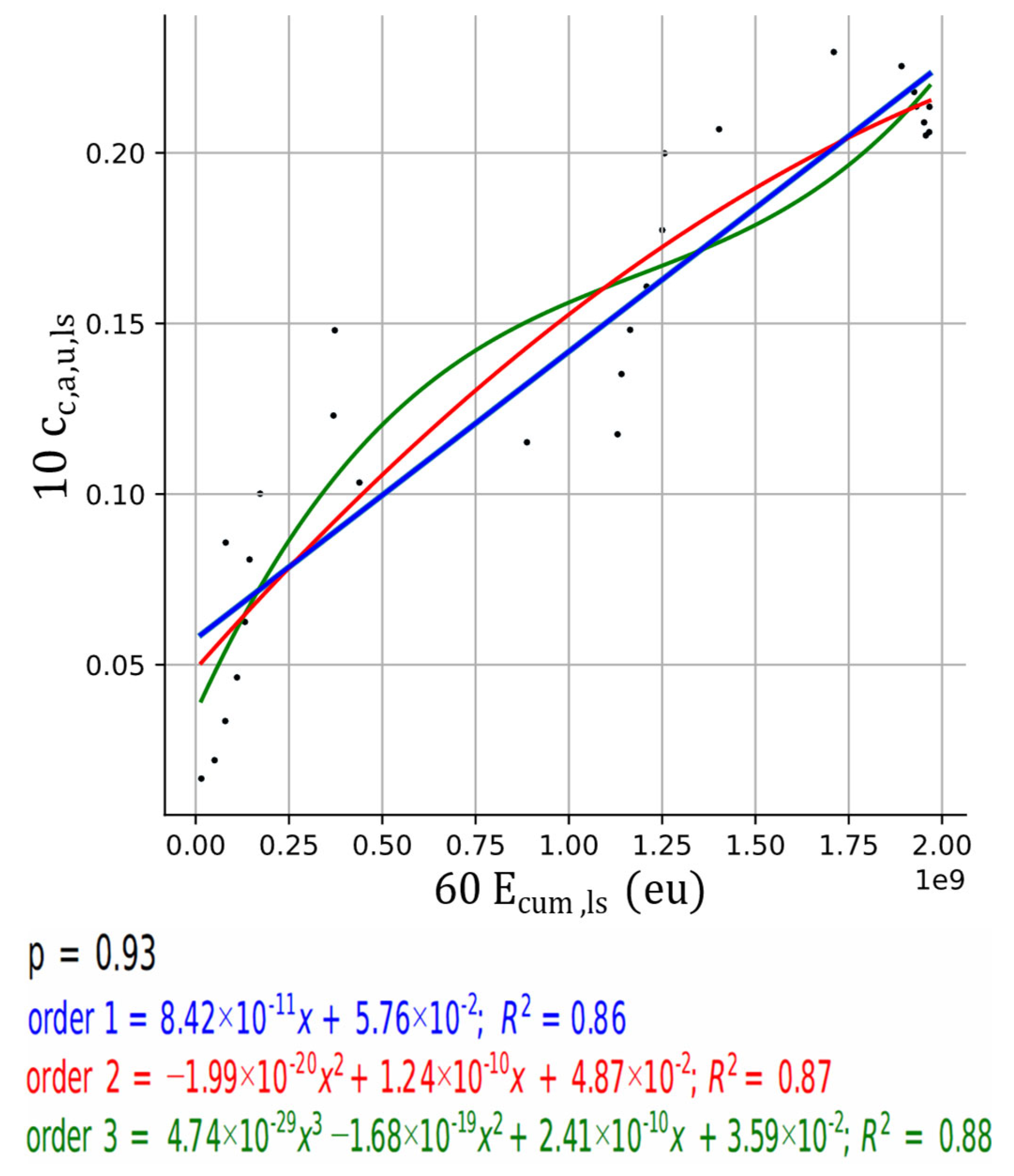
The acoustic signatures that best captured this intermediate state were the early transitoriness ( e T r a , u , l s , ID = 52), for ω c = 3%, Figure 18, and the cumulative acoustic energy ( E c u m , l s , ID = 60), for ω c = 6%, Figure 19, with values of | p | ≥ 0.89. This statistically corroborates the lubricating effect of water in soil mechanics: at intermediate moisture contents, the fluid optimally lubricates the silica grains, facilitating smoother, lower-energy sliding and rearrangement. Consequently, the acoustic emissions become highly sensitive markers of the soil’s inherent deformability and compressibility rather than just the raw stress applied.
As discussed at the beginning of this block, integrating the well-graded composite ( S 4 ) into the analysis yielded virtually identical trends, proving that this moisture-dependent shift from stress-driven to deformability-driven acoustic signatures is a universal phenomenon across both uniform and heterogeneous soil matrices.

3.4. Block 4: The Dynamics of Stress Levels

The compression of a granular matrix is a highly dynamic, non-linear thermodynamic process. The physical mechanisms responsible for generating elastic waves evolve as the state of stress escalates. To map these shifts mathematically, this analytical block partitions the dataset into three discrete regimes—low, medium, and high stress—and executes a dual analysis for each: a holistic evaluation of all vibrated samples ( S 1 through S 4 at all moistures), followed by a confrontation between dry vibrated and dry non-vibrated matrices.
The reference thresholds for each stress level—low σ v , l , medium ( σ v , m ), and high ( σ v , h )—correspond to representative effective vertical stress values derived from loading stages 2 (l), 5 (m), and 8 (h) of Table 1, respectively. In this framework, the representative value for each stage is defined as 160% of the initial stress value of the aforementioned stage. Consequently, the established reference stresses for the predictive models are σ v , l = 40 kN/m2, σ v , m = 320 kN/m2, and σ v , h = 2560 kN/m2. These discrete regimes allow for the identification of the dominant geomechanical phenomena in each phase: from the initial spatial reorganisation and grain sliding at low stresses to the progressive onset of abrasive friction and eventual grain microcracking as the stress reaches the upper limit of the high-stress domain [38,39].

3.4.1. Global Trends in Vibrated Matrices

Across all three stress domains, the multivariate analysis of the vibrated samples successfully identified robust correlations, indicating that predictive capabilities are maintained throughout the entire loading history. However, a deeper phenomenological transition was observed in the parameters providing the highest predictive accuracy:
  • Low Stress Level ( σ v , l = 40 kN/m2): In the early stages of loading, the soil skeleton undergoes primary consolidation dominated by kinematic particle rearrangement. During this phase, the compression index ( c c , l s , ID = 9) and the coefficient of compressibility ( a v , l s , ID = 13) exhibited excellent ( p = 0.76), predominantly positive correlations with the number of AE hits ( N H i t l s , ID = 14); Table 10. Physically, this demonstrates that highly compressible, initially porous soils will undergo extensive spatial reorganisation, generating a massive barrage of low-energy friction and sliding events. At this stage, counting the sheer volume of discrete acoustic emissions ( N H i t ) is the most reliable method for predicting the soil’s early deformability.
  • Medium Stress Level ( σ v , m = 320 kN/m2): As the effective stress progresses, the granular matrix becomes highly interlocked. The dominant acoustic mechanism shifts from widespread rearrangement towards intense point-to-point asperity abrasion. Here, the highest statistical correlations for the compression index ( c c , l s , ID = 9) and stage strain ( ε l s , ID = 12) shifted from the hit count to the peak amplitude ( A l s , ID = 15) and the average early transitoriness ( e T r a , u , l s , ID = 52), Table 11, with values of | p | ≥ 0.76. Additionally, the coefficient of compressibility ( a v , l s , ID = 13) presented strong negative correlations ( p = −0.80) with the peak amplitude ( A l s , ID = 15). This mathematically corroborates that as a soil densifies and becomes less compressible (lower a v ), the intense energy released from the abrasion of newly locked asperities leads to markedly higher acoustic amplitudes.
  • High Stress Level ( σ v , h = 2560 kN/m2): At extreme boundary loads, pervasive grain microcracking commences. In this regime, the coefficient of compressibility ( a v , l s ) tends asymptotically towards a residual, minimal value, severely weakening its statistical relationship with the acoustic parameters. Instead, the average compression index ( c c , a , u , l s , ID = 10) and the loading stage strain ( ε l s , ID = 12) maintain robust predictability, correlating predominantly with the average amplitude ( A a , u , l s , ID = 16) and the early transitoriness ( e T r a , u , l s , ID = 52), Table 12, with values of | p | ≥ 0.75. This validates that under massive structural loads, the raw amplitude of the transient fractures dictates the acoustic profile.

3.4.2. The Convergence of Initial Fabric at High Stresses

The second phase of this block focused strictly on dry soils ( ω c = 0%), contrasting the behaviour of structurally locked (vibrated) and meta-stable (non-vibrated) matrices at the three specific stress thresholds. The reader should note that in these specific sub-analyses, the number of samples tested—and consequently the volume of available data points—is considerably smaller than in the aggregate analyses presented thus far. This reduction in the sample size ( n ) naturally leads to a notable increase in the Pearson correlation coefficients ( p ), as the statistical variance is narrowed within a more constrained experimental population.
At the low stress level ( σ v , l = 40 kN/m2), a profound statistical disparity was evident. The non-vibrated samples, lacking initial interlocking, suffered massive macroscopic volumetric collapse upon the application of the load. This catastrophic early settlement generated highly erratic, noisy acoustic wave trains that fundamentally hindered the derivation of clean statistical models; Table 13. Conversely, the vibrated matrices, possessing a stable initial fabric, transferred the boundary load efficiently, maintaining high predictive correlations (Table 14).
However, as the evaluation moved to the medium ( σ v , m = 320 kN/m2) and ultimately the high stress level ( σ v , h = 2560 kN/m2), this statistical gap narrowed significantly and effectively vanished (Table 15, Table 16, Table 17 and Table 18). By the time the non-vibrated soils reached 2560 kN/m2, the sheer magnitude of the applied compression had forcefully destroyed their meta-stable fabric, densifying them to a state nearly identical to that of the initially vibrated samples. Consequently, under extreme pressures, the acoustic signatures of both starting states became statistically indistinguishable, governed exclusively by pervasive grain microcracking.
This finding establishes a crucial design parameter for structural health monitoring: while ensuring proper initial compaction is vital for accurately predicting soil behaviour beneath shallow foundations (low-to-medium stress), acoustic emission models deployed for extreme-pressure environments—such as deep pile tips or tectonic fault zones—are highly resilient to variations in the soil’s initial depositional fabric.

3.5. Block 5: The Influence of Initial Fabric in Dry Soils

While moisture content plays a critical role in acoustic wave attenuation, the structural organisation of the soil grains prior to loading—the initial fabric—fundamentally dictates the internal stress distribution. To meticulously isolate and quantify the effect of the initial compaction state on the generation of acoustic emissions, this final block evaluates exclusively dry soil matrices ( ω c = 0%). A direct statistical confrontation was executed between mechanically vibrated dry soils (samples S 1 / 1, S 2 /1, S 3 /1, and S 4 /1) and non-vibrated, loosely poured dry soils (samples S 1 / 6, S 2 /6, S 3 /6, and S 4 /6).
For both fabric states, the multivariate analysis revealed that each monitored geotechnical variable possessed at least a moderate correlation ( | p | ≥ 0.51) with specific acoustic parameters; Table 19 and Table 20. However, when removing the initial state variables (initial dry density, ρ d , 0 , ID = 3, and initial void ratio, e 0 , ID = 4) from the non-vibrated subset (Table 20), the minimum correlation degree rose significantly to p = 0.62, indicating that the vast majority of variables presented high ( | p | ≥ 0.60) to very high ( | p | ≥ 0.80) correlation degrees.
A direct comparison of the Pearson correlation coefficients ( p ) between the two subsets yielded critical insights into the acoustic behaviour of granular materials:
Predictive Superiority of Vibrated Matrices: The mechanically vibrated soils globally presented slightly superior correlation coefficients compared to their non-vibrated counterparts. Specifically, the vibrated soils yielded very high correlations ( | p | ≥ 0.80) for five key geotechnical variables: characteristic grain size ( ϕ s , ID = 1), logarithmic effective stress ( log 10 ( σ l s ) , ID = 6), weighted average compression index ( c c , w a , u , l s , ID = 11), stage strain ( ε l s , ID = 12), and the coefficient of compressibility ( a v , l s , ID = 13); Table 19. In contrast, the non-vibrated soils only reached this very high correlation threshold for three variables log 10 ( σ l s ) , c c , a , u , l s (ID = 10), and c c , w a , u , l s , Table 20.
The Impact of Initial Compaction: The disparity between the two states was particularly pronounced for the initial state variables ( ρ d , 0 and e 0 ). The absence of mechanical vibration prior to testing resulted in a poor, meta-stable spatial arrangement of the grains (loose fabric). This lack of structural interlocking significantly altered the acoustic results compared to the properly vibrated samples. Since properly vibrated and compacted soils generally better replicate the in situ geomechanical behaviour of natural deposits, their acoustic signatures are deemed much more reliable for establishing empirical predictive models.
Dominant Acoustic Signatures in Dry Soils: For the vibrated dry soils (Table 19), specific acoustic parameters consistently emerged as the most reliable predictors of the soil state. The cumulative signal strength ( S s , c u m , l s , ID = 61) demonstrated a highly robust correlation ( | p | ≥ 0.73) with the effective stress (both σ l s , ID = 5, and log 10 ( σ l s ) , the loading stage strain ( ε l s , ID = 12), and the compression indices ( c c , a , u , l s , c c , w a , u , l s ). Meanwhile, the initial fabric states ( ρ d , 0 , ID = 3, and e 0 , ID = 4) were best inferred from the average peak amplitude ( A a , u , l s , ID = 16). Finally, the weighted average b-value ( b w a , u , l s , ID = 56)—which tracks the proportion of high-amplitude to low-amplitude events—acted as an excellent predictor for the dynamic evolution of the soil’s coefficient of compressibility ( a v , l s , ID = 13).

4. Conclusions

The present research establishes a robust multivariate mathematical framework for the non-destructive characterisation of granular soil states through the lens of statistical complexity. By integrating 61 variables across diverse geomechanical and acoustic domains, this study demonstrates that the stochastic energy release within the granular skeleton is governed by structured, predictable patterns. The main findings are summarised below:

4.1. Generalised Findings and Global Predictive Feasibility

  • Holistic Predictability: A fundamental conclusion of this work is the confirmation that all 13 geomechanical state parameters can be inferred with high statistical significance through acoustic signatures. The multivariate architecture achieved Pearson coefficients p exceeding 0.80 for the majority of target-predictor pairs, validating the transition from qualitative monitoring to quantitative predictive modelling.
  • Recurrent Geotechnical Targets: The variables that emerged as the most consistently predictable across all analytical blocks were the vertical effective stress ( σ l s ), the initial void ratio ( e 0 ) and dry density ( ρ d , 0 ), the loading stage strain ( ε l s ) and the compression index ( c c ). Their strong correlation with acoustic activity confirms that volumetric changes and stress increments are the primary drivers of energy dissipation in the sample matrix.
  • Recurrent Acoustic Predictors: In terms of predictive power, the Signal Strength ( S s ) and Acoustic Energy ( E ), particularly in their cumulative ( S s , c u m , l s and E c u m , l s ) and weighted forms ( S s , w a , u , l s and E w a , u , l s ), as well as the signal amplitude ( A ), were the most recurrently selected predictors. The weighted average b-value ( b w a , u , l s ) effectively predicted the dynamic evolution of the soil’s coefficient of compressibility ( a v , l s ). Additionally, the dimensionless parameter earliness ( e a r l ) proved to be an essential descriptor for capturing the stationarity and symmetry of the waveforms during structural rearrangement.

4.2. Block-Specific Conclusions

  • Block 1 (Generalised Baseline): Establishing a universal baseline using mechanically vibrated samples confirms that log 10 ( σ l s ) is the supreme driver of the acoustic response.
  • Block 2 (Soil Typology): Particle size distribution ( D 30 ) dictates the “frequency fingerprint” of the soil since the coarser fractions ( S 3 ) generate higher-amplitude events linked to kinematic instability and the onset of micro-cracking, while the finer fractions ( S 1 ) tend to produce higher-frequency signatures associated with abrasive friction. In this regard, it was observed that the presence of interstitial fluid facilitates smooth, low-energy grain sliding, drastically reducing the emission of high-amplitude transient hits.
  • Block 3 (Moisture and Lubrication): The interstitial fluid acts as a critical thermodynamic regulator. Increasing moisture content from 0% to 12% results in a systematic reduction in acoustic energy release due to the lubricating effect, which “softens” inter-granular contacts and reduces the complexity of the emitted signals.
  • Block 4 (Stress-Dependent Acoustic Evolution): The analysis of the three stress regimes reveals a clear transition in the dominant geomechanical mechanisms and their corresponding acoustic signatures. At low stress levels (40 kN/m2), the soil’s early deformability is best captured by the volume of events ( N H i t l s ), reflecting massive spatial reorganisation. As the matrix densifies at medium stress (320 kN/m2), a strong negative correlation ( p = −0.80) between compressibility ( a v ) and amplitude ( A l s ) emerges, indicating that the locking of asperities shifts the energy release toward higher-intensity friction. Finally, under high stress (2560 kN/m2), the acoustic profile is dictated by the raw amplitude of transient fractures, validating that the energetic magnitude of microcracking becomes the primary descriptor of structural failure.
  • Block 4 (Influence of Initial Fabric and Structural Convergence): This study identifies a profound statistical disparity at low stress levels (40 kN/m2) based on initial soil fabric; while vibrated matrices maintain high predictive stability, non-vibrated samples undergo a catastrophic volumetric collapse that generates erratic, noisy wave trains, hindering precise modelling. However, this initial structural influence is not permanent. By the high stress regime (2560 kN/m2), the magnitude of the applied load forcefully destroys the meta-stable fabric of non-vibrated soils, densifying them to a state nearly identical to vibrated samples. Consequently, under extreme pressures, the acoustic signatures of both starting states converge and become statistically indistinguishable, governed exclusively by pervasive grain microcracking.
  • Block 5 (Initial Fabric): Structural compaction is a primary boundary condition. Mechanically vibrated matrices exhibit a more “ordered” acoustic response compared to non-vibrated matrices. The initial void ratio ( e 0 ) and initial dry density ( ρ d , 0 ) are effectively predicted via the average RA ( R A a , u , l s ) in dry non-vibrated soils and the average peak amplitude ( A a , u , l s ) in dry vibrated soils, confirming that initial packing dictates the system’s potential energy release.

4.3. Final Remarks

Ultimately, this research demonstrates that the application of high-order polynomial regressions and multi-scale temporal aggregation ( P l s , P a , u , l s , and P w a , u , l s ) provides a superior mathematical architecture for geomechanical inference. The transition from “Acoustic Emission monitoring” to “Statistical Complexity modelling” opens new avenues for the in situ characterisation of intricate geological domains, providing a non-destructive gateway into the hidden dynamics of the granular world.

Supplementary Materials

The following supporting information can be downloaded at: https://www.mdpi.com/article/10.3390/sym18060940/s1. Table S1. Geotechnical and acoustic parameters corresponding to sample S1/1. Table S2. Geotechnical and acoustic parameters corresponding to sample S1/2. Table S3. Geotechnical and acoustic parameters corresponding to sample S1/3. Table S4. Geotechnical and acoustic parameters corresponding to sample S1/4. Table S5. Geotechnical and acoustic parameters corresponding to sample S1/5. Table S6. Geotechnical and acoustic parameters corresponding to sample S1/6. Table S7. Geotechnical and acoustic parameters corresponding to sample S2/1. Table S8. Geotechnical and acoustic parameters corresponding to sample S2/2. Table S9. Geotechnical and acoustic parameters corresponding to sample S2/3. Table S10. Geotechnical and acoustic parameters corresponding to sample S2/4. Table S11. Geotechnical and acoustic parameters corresponding to sample S2/5. Table S12. Geotechnical and acoustic parameters corresponding to sample S2/6. Table S13. Geotechnical and acoustic parameters corresponding to sample S3/1. Table S14. Geotechnical and acoustic parameters corresponding to sample S3/2. Table S15. Geotechnical and acoustic parameters corresponding to sample S3/3. Table S16. Geotechnical and acoustic parameters corresponding to sample S3/4. Table S17. Geotechnical and acoustic parameters corresponding to sample S3/5. Table S18. Geotechnical and acoustic parameters corresponding to sample S3/6. Table S19. Geotechnical and acoustic parameters corresponding to sample S4/1. Table S20. Geotechnical and acoustic parameters corresponding to sample S4/2. Table S21. Geotechnical and acoustic parameters corresponding to sample S4/3. Table S22. Geotechnical and acoustic parameters corresponding to sample S4/4. Table S23. Geotechnical and acoustic parameters corresponding to sample S4/5. Table S24. Geotechnical and acoustic parameters corresponding to sample S4/6.

Author Contributions

G.G.-R.: Conceptualisation, Data curation, Formal analysis, Investigation, Methodology, Project administration, Resources, Software, Supervision, Validation, Visualisation, Writing—original draft, and Writing—review and editing; J.F.S.-P.: Conceptualisation, Data curation, Funding acquisition, Project administration, Resources, Software, Supervision, Validation, and Writing—review and editing; E.C.: Data curation, Formal analysis, Funding acquisition, Investigation, Methodology, Project administration, Resources, Software, Supervision, Validation, and Writing—review and editing; D.X.V.-L.: Conceptualisation, Data curation, Formal analysis, Investigation, Software, Validation, Visualisation, Writing—original draft, and Writing—review and editing; M.C.: Formal analysis, Methodology, Software, Validation, Writing—original draft, and Writing—review and editing; J.J.: Formal analysis, Validation, Visualisation, and Writing—review and editing. All authors have read and agreed to the published version of the manuscript.

Funding

This research received no external funding.

Data Availability Statement

The original contributions presented in this study are included in the article/Supplementary Material. Further inquiries can be directed to the corresponding authors.

Conflicts of Interest

The authors declare no conflicts of interest.

References

  1. Koerner, R.M.; Curran, J.W.; Mccabe, W.M.; Lord, A.E., Jr. Acoustic emission behavior of granular soils. J. Geotech. Eng. Div. 1976, 102, 761–773. [Google Scholar] [CrossRef]
  2. Naderi-Boldaji, M.; Bahrami, M.; Keller, T.; Or, D. Characteristics of acoustic emissions from soil subjected to confined uniaxial compression. Vadose Zone J. 2017, 16, 1–12. [Google Scholar] [CrossRef]
  3. Michlmayr, G.; Or, D. Mechanisms for acoustic emissions generation during granular shearing. Granul. Matter 2014, 16, 627–640. [Google Scholar] [CrossRef]
  4. Frid, V.; Potirakis, S.M.; Shulov, S. Study of static and dynamic properties of sand under low stress compression. Appl. Sci. 2021, 11, 3311. [Google Scholar] [CrossRef]
  5. Lin, W.; Liu, A.; Mao, W. Use of acoustic emission to evaluate the micro-mechanical behavior of sands in single particle compression tests. Ultrasonics 2019, 99, 105962. [Google Scholar] [CrossRef] [PubMed]
  6. Muñoz-Ibáñez, A.; Delgado-Martín, J.; Grande-García, E. Acoustic emission processes occurring during high-pressure sand compaction. Geophys. Prospect. 2019, 67, 761–783. [Google Scholar] [CrossRef]
  7. Mao, W.; Yang, Y.; Lin, W.; Aoyama, S.; Towhata, I. High frequency acoustic emissions observed during model pile penetration in sand and implications for particle breakage behavior. Int. J. Geomech. 2018, 18, 04018143. [Google Scholar] [CrossRef]
  8. Michlmayr, G.; Cohen, D.; Or, D. Sources and characteristics of acoustic emissions from mechanically stressed geologic granular media—A review. Earth. Sci. Rev. 2012, 112, 97–114. [Google Scholar] [CrossRef]
  9. Lockner, D. The role of acoustic emission in the study of rock fracture. Int. J. Rock Mech. Min. Sci. Geomech. Abstr. 1993, 30, 883–899. [Google Scholar] [CrossRef]
  10. Labuz, J.F.; Cattaneo, S.; Chen, L.H. Acoustic emission at failure in quasi-brittle materials. Constr. Build. Mater. 2001, 15, 225–233. [Google Scholar] [CrossRef]
  11. Tanimoto, K.; Tanaka, Y. Yielding of soil as determined by acoustic emission. Soils Found. 1986, 26, 69–80. [Google Scholar] [CrossRef]
  12. Aggelis, D.G.; Soulioti, D.V.; Sapouridis, N.; Barkoula, N.M.; Paipetis, A.S.; Matikas, T.E. Acoustic emission characterization of the fracture process in fibre reinforced concrete. Constr. Build. Mater. 2011, 25, 4126–4131. [Google Scholar] [CrossRef]
  13. Frid, V.; Potirakis, S.M.; Shulov, S. Effect of soil loading and unloading on its acoustic behavior. Proc. West. Mark. Ed. Assoc. Conf. 2020, 67, 20. [Google Scholar] [CrossRef]
  14. Carneiro, R.F.; Gerscovich, D.M.S.; Danziger, B.R. Reconstructing oedometric compression curves for selecting design parameters. Can. Geotech. J. 2019, 56, 621–635. [Google Scholar] [CrossRef]
  15. Gao, M.; Yan, H.; Duan, H.; Xiong, S. Experimental study on coal specimens subjected to uniaxial cyclic loading and unloading. Appl. Sci. 2022, 12, 11810. [Google Scholar] [CrossRef]
  16. Lord, A.E.; Koerner, R.M. In-Situ Stress Determination in Soil and Rock Using the Acoustic Emission Method; National Bureau of Standards: Philadelphia, PA, USA, 1984. [Google Scholar] [CrossRef]
  17. Ono, K. Acoustic Emission. In Springer Handbook of Acoustics; Rossing, T.D., Ed.; Springer: New York, NY, USA, 2014; pp. 1209–1229. [Google Scholar] [CrossRef]
  18. Lord, A.E., Jr. Acoustic emission. Phys. Acoust. 1975, 11, 289–353. [Google Scholar] [CrossRef]
  19. Gallego, A.; Martínez, E. Emisión Acústica. Niveles I y II (Ensayos no Destructivos-AEND); FC Editorial: Madrid, Spain, 2015. [Google Scholar]
  20. Villalva-León, D.X.; García-Ros, G.; Sánchez-Pérez, J.F.; Castro-Rodríguez, E.; Mena-Requena, M.R.; Conesa, M. An Overview of the Study of Acoustic Emissions in Soil Mechanics. In Proceedings of the 8th World Congress on Mechanical, Chemical, and Material Engineering (MCM’22), Prague, Czech Republic, 31 July–2 August 2022. [Google Scholar] [CrossRef]
  21. Ohtsu, M.; Watanabe, H. Quantitative damage estimation of concrete by acoustic emission. Constr. Build. Mater. 2001, 15, 217–224. [Google Scholar] [CrossRef]
  22. Shigeishi, M.; Colombo, S.; Broughton, K.J.; Rutledge, H.; Batchelor, A.J.; Forde, M.C. Acoustic emission to assess and monitor the integrity of bridges. Constr. Build. Mater. 2001, 15, 35–49. [Google Scholar] [CrossRef]
  23. Zhu, H.; Liu, F.; Cui, J.; Peng, W. Research on tunnel damage process based on acoustic emission technology. J. Phys. Conf. Ser. 2022, 2196, 012001. [Google Scholar] [CrossRef]
  24. Michlmayr, G.; Chalari, A.; Clarke, A.; Or, D. Fiber-optic high-resolution acoustic emission (AE) monitoring of slope failure. Landslides 2017, 14, 1139–1146. [Google Scholar] [CrossRef]
  25. Aggelis, D.G.; Shiotani, T. Parameters Based AE Analysis. In Acoustic Emission Testing; Grosse, C.U., Ohtsu, M., Aggelis, D.G., Shiotani, T., Eds.; Springer Tracts in Civil Engineering; Springer: Berlin/Heidelberg, Germany, 2022; pp. 45–71. [Google Scholar] [CrossRef]
  26. Barile, C.; Casavola, C.; Pappalettera, G.; Kannan, V.P. Application of different acoustic emission descriptors in damage assessment of fiber reinforced plastics: A comprehensive review. Eng. Fract. Mech. 2020, 235, 107083. [Google Scholar] [CrossRef]
  27. Sagar, R.V.; Prasad, B.R. A review of recent developments in parametric based acoustic emission techniques applied to concrete structures. Nondestruct. Test. Eval. 2012, 27, 47–68. [Google Scholar] [CrossRef]
  28. Schumacher, T.; Linzer, L.; Grosse, C.U. Signal-based AE analysis. In Acoustic Emission Testing: Basics for Research–Applications in Engineering; Grosse, C.U., Ohtsu, M., Aggelis, D.G., Shiotani, T., Eds.; Springer: Berlin/Heidelberg, Germany, 2022; pp. 73–116. [Google Scholar] [CrossRef]
  29. Ohtsu, M. Source kinematics of acoustic emission based on a moment tensor. NDT Int. 1989, 22, 14–20. [Google Scholar] [CrossRef]
  30. Ren, Y.; Vavryčuk, V.; Wu, S.; Gao, Y. Accurate moment tensor inversion of acoustic emissions and its application to Brazilian splitting test. Int. J. Rock Mech. Min. Sci. 2021, 141, 104707. [Google Scholar] [CrossRef]
  31. Zhang, Z.; Ma, K.; Li, H.; He, Z. Microscopic investigation of rock direct tensile failure based on statistical analysis of acoustic emission waveforms. Rock Mech. Rock Eng. 2022, 55, 2445–2458. [Google Scholar] [CrossRef]
  32. Li, G.; Zhang, H.; Li, M.; Shen, Z.; Tian, A.; Wang, L. Study on coal wall spalling mechanism of large mining height working face based on folding mutation theory. Sci. Rep. 2026, 16, 15277. [Google Scholar] [CrossRef] [PubMed]
  33. Hou, Y.; Miao, C.; Zhu, C.; Li, Z.; Du, F.; Wang, W.; Yang, X.; Cao, Z. Flow Mechanism of Grouting Slurry in Rough Fracture Based on CFD-DEM Coupling Method. Processes 2026, 14, 1307. [Google Scholar] [CrossRef]
  34. Castro, E.; García-Ros, G.; Villalva-León, D.X.; Valenzuela, J.; Sánchez-Pérez, J.F.; Conesa, M. Dimensionless Parameters for Waveform Characterization of Acoustic Emission Signals: Application to Sedimentation and Soil Compression Experiments. Symmetry 2023, 15, 2094. [Google Scholar] [CrossRef]
  35. García-Ros, G.; Villalva-León, D.X.; Castro, E.; Sánchez-Pérez, J.F.; Valenzuela, J.; Conesa, M. Multivariate Statistical and Correlation Analysis between Acoustic and Geotechnical Variables in Soil Compression Tests Monitored by the Acoustic Emission Technique. Mathematics 2023, 11, 4085. [Google Scholar] [CrossRef]
  36. ASTM D2435-04; Standard Test Methods for One-Dimensional Consolidation Properties of Soils Using Incremental Loading. ASTM: West Conshohocken, PA, USA, 2011.
  37. ASTM D854-14; Standard Test Methods for Specific Gravity of Soil Solids by Water Pycnometer. ASTM: West Conshohocken, PA, USA, 2023.
  38. UNE-EN 1330-9; Ensayos no destructivos. Terminología. Parte 9: Términos utilizados en ensayos de emisión acústica. Asociación Española de Normalización (UNE): Madrid, Spain, 2018.
  39. Manthei, G.; Eisenblätter, J. Acoustic Emission in Study of Rock Stability. In Acoustic Emission Testing: Basics for Research–Applications in Engineering; Springer: Berlin/Heidelberg, Germany, 2008; pp. 239–310. [Google Scholar] [CrossRef]
  40. Dong, L.; Zhang, L.; Liu, H.; Du, K.; Liu, X. Acoustic emission b value characteristics of granite under true triaxial stress. Mathematics 2022, 10, 451. [Google Scholar] [CrossRef]
  41. Wang, C.; Du, G.; Han, Y.; He, K.; Li, E. Evolution characteristics of acoustic emission and strain energy for deep granite under different damage stages. Geomech. Geophys. Geo-Energy Geo-Resour. 2023, 9, 14. [Google Scholar] [CrossRef]
  42. Cui, Y.; Xue, L.; Zhai, M.; Xu, C.; Bu, F.; Wan, L. Experimental investigation on the influence on mechanical properties and acoustic emission characteristics of granite after heating and water-cooling cycles. Geomech. Geophys. Geo-Energy Geo-Resour. 2023, 9, 88. [Google Scholar] [CrossRef]
  43. Caso, E.; Díez-Ibarbia, A.; García, P.; Sánchez-Espiga, J.; Fernández-del-Rincón, A. Evaluation of acoustic emission for monitoring wire drawing process. Mech. Syst. Signal Process. 2023, 200, 110598. [Google Scholar] [CrossRef]
  44. Yan, L.; Han, B.; Zhang, L.; Li, W.; Xie, H.; Gao, C.; Chen, L.; Yu, J.; Song, Z.; Zuo, B. Experimental study on fatigue damage of continuous steel–concrete composite beam by acoustic emission. Structures 2023, 57, 105185. [Google Scholar] [CrossRef]
  45. Gutenberg, B.; Richter, C. Seismicity of the Earth; Geological Society of America: Boulder, CO, USA, 1941; Volume 34. [Google Scholar]
  46. Benioff, H.; Gutenberg, B.; Press, F.; Richter, C.F. Progress Report, Seismological Laboratory of the California Institute of Technology. Eos Trans. Am. Geophys. Union 1957, 39, 721–725. [Google Scholar] [CrossRef]
  47. Hall, S.A.; de Sanctis, F.; Viggiani, G. Monitoring fracture propagation in a soft rock (Neapolitan Tuff) using acoustic emissions and digital images. Pure Appl. Geophys. 2006, 163, 2171–2204. [Google Scholar] [CrossRef]
  48. Ono, K. Current understanding of mechanisms of acoustic emission. J. Strain Anal. Eng. Des. 2005, 40, 1–15. [Google Scholar] [CrossRef]
Figure 1. Particle size distribution profiles of the four quartz-rich coastal sand samples investigated.
Symmetry 18 00940 g001
Figure 2. Schematic diagram of the experimental setup.
Symmetry 18 00940 g002
Figure 3. Electronic position transducer (Gefran PY-2-C-010) utilised to map vertical settlement.
Symmetry 18 00940 g003
Figure 4. Electronic load cell (AEP Transducers TS 1t C3) utilised to quantify the external stress applied to the sample.
Symmetry 18 00940 g004
Figure 5. Placement of the low-frequency (the larger of the two) and broadband (the shorter) piezoelectric sensors at the base of the oedometric cell.
Symmetry 18 00940 g005
Figure 6. Regression functions and trend lines for the correlation between log10(σ’ls) and F l s . All mechanically vibrated soil samples.
Symmetry 18 00940 g006
Figure 7. Regression functions and trend lines for the correlation between log10(σ’ls) and F a , u , l s . All vibrated soil samples S 2 .
Symmetry 18 00940 g007
Figure 8. Regression functions and trend lines for the correlation between log10(σ’ls) and C N T S w a , u , l s . All vibrated soil samples S 3 .
Symmetry 18 00940 g008
Figure 9. Regression functions and trend lines for the correlation between log10(σ’ls) and F a , u , l s . All vibrated soil samples S 4 .
Symmetry 18 00940 g009
Figure 10. Regression functions and trend lines for the correlation between ω c and b a , u , l s . All vibrated soil samples S 1 .
Symmetry 18 00940 g010
Figure 11. Regression functions and trend lines for the correlation between ϕ s and C N T S a , u , l s . All vibrated soil samples S 1 and S 4 .
Symmetry 18 00940 g011
Figure 12. Regression functions and trend lines for the correlation between ϕ s and A a , u , l s . All vibrated soil samples S 2 and S 4 .
Symmetry 18 00940 g012
Figure 13. Regression functions and trend lines for the correlation between ϕ s and E a , u , l s . All vibrated soil samples S 3 and S 4 .
Symmetry 18 00940 g013
Figure 14. Regression functions and trend lines for the correlation between ϕ s and T r a , u , l s . All vibrated soil samples S 1 , S 2 and S 3 .
Symmetry 18 00940 g014
Figure 15. Regression functions and trend lines for the correlation between log 10 ( σ l s ) and C N T S a , u , l s . Vibrated soil samples S 1 , S 2 , and S 3 with ω c = 0%.
Symmetry 18 00940 g015
Figure 16. Regression functions and trend lines for the correlation between log 10 ( σ l s ) and S s , c u m , l s . Vibrated soil samples S 1 , S 2 , and S 3 with ω c = 9%.
Symmetry 18 00940 g016
Figure 17. Regression functions and trend lines for the correlation between log 10 ( σ l s ) and F a , u , l s . Vibrated soil samples S 1 , S 2 , and S 3 with ω c = 12%.
Symmetry 18 00940 g017
Figure 18. Regression functions and trend lines for the correlation between c c , w a , u , l s and e T r a , u , l s . Vibrated soil samples S 1 , S 2 , and S 3 with ω c = 3%.
Symmetry 18 00940 g018
Figure 19. Regression functions and trend lines for the correlation between c c , a , u , l s and E c u m , l s . Vibrated soil samples S 1 , S 2 , and S 3 with ω c = 6%.
Symmetry 18 00940 g019
Table 1. Comprehensive summary of the initial state variables ( G s , e 0 , ρ d , 0 ) and starting conditions for the 24 discrete soil samples tested.
Soil/Test ID ω c (%)Vibrated (v) or
Non-Vibrated (nv)
G s ρ d , 0 (g/cm3) e 0
S 1 /10v2.761.910.45
S 1 /23v1.181.34
S 1 /36v1.251.21
S 1 /49v1.341.06
S 1 /512v1.550.78
S 1 /60nv1.770.56
S 2 /10v2.731.740.57
S 2 /23v1.311.08
S 2 /36v1.281.13
S 2 /49v1.370.99
S 2 /512v1.480.84
S 2 /60nv1.660.64
S 3 /10v2.811.850.52
S 3 /23v1.610.75
S 3 /36v1.560.8
S 3 /49v1.620.73
S 3 /512v1.750.61
S 3 /60nv1.820.54
S 4 /10v2.782.040.36
S 4 /23v1.460.90
S 4 /36v1.520.83
S 4 /49v1.820.53
S 4 /512v2.130.31
S 4 /60nv1.990.40
Table 2. Discrete stress thresholds defining the nine loading stages ( l s ) used for processing and further study of the data obtained in the compression tests.
Load Step Identifier (Ordinal Number)Initial and Final Effective Stress (kN/m2)
σ v , i σ v , f
Load Step Identifier (ls)
(Final Effective Stress)
preload0–12.5-
112.5–2525
225–5050
350–100100
4100–200200
5200–400400
6400–800800
7800–16001600
81600–32003200
93200–>50005000
Table 3. Macroscopic geotechnical variables monitored for the multivariate analysis [34,35].
IDSymbolUnitsDescription
1 ϕ s mmCharacteristic grain size (diameter)
2 ω c %Moisture content
3 ρ d , 0 g/cm3Initial dry density
4 e 0 (dimensionless)Initial void ratio
5 σ l s kN/m2Loading stage effective stress
6 log 10 ( σ l s ) -Logarithm of the loading stage effective stress
7 ρ d , l s g/cm3Loading stage dry density
8 e l s (dimensionless)Loading stage void ratio
9 c c , l s -Loading stage compression index
10 c c , a , u , l s -Average compression index up to the loading stage
11 c c , w a , u , l s -Weighted average compression index up to the loading stage
12 ε l s (dimensionless)Loading stage strain
13 a v , l s m2/kNLoading stage coefficient of compressibility
Table 4. Acoustic emission (AE) variables monitored for the multivariate analysis.
IDSymbolUnitsDescription
14 N H i t l s (units)Number of hits of the loading stage
15 A l s dBLoading stage peak amplitude
16 A a , u , l s dBAverage peak amplitude up to the loading stage
17 A w a , u , l s dBWeighted average peak amplitude up to the loading stage
18 A v , l s mVLoading stage true linear amplitude
19 A v , a , u , l s mVAverage true linear amplitude up to the loading stage
20 A v , w a , u , l s mVWeighted average true linear amplitude up to the loading stage
21 D l s µsLoading stage signal duration
22 D a , u , l s µsAverage signal duration up to the loading stage
23 D w a , u , l s µsWeighted average signal duration up to the loading stage
24 C N T S l s (units)Loading stage average counts number
25 C N T S a , u , l s (units)Average counts up to the loading stage
26 C N T S w a , u , l s (units)Weighted average counts up to the loading stage
27 F l s kHzLoading stage frequency
28 F a , u , l s kHzAverage frequency up to the loading stage
29 F w a , u , l s kHzWeighted average frequency up to the loading stage
30 R T l s µsLoading stage rise time
31 R T a , u , l s µsAverage rise time up to the loading stage
32 R T w a , u , l s µsWeighted average rise time up to the loading stage
33 E l s V2sLoading stage acoustic energy
34 E a , u , l s V2sAverage acoustic energy up to the loading stage
35 E w a , u , l s V2sWeighted average acoustic energy up to the loading stage
36 S s , l s VsLoading stage signal strength
37 S s , a , u , l s VsAverage signal strength up to the loading stage
38 S s , w a , u , l s VsWeighted average signal strength up to the loading stage
39 S s , p , l s VsLoading stage peak signal strength
40 S s , p , a , u , l s VsAverage peak signal strength up to the loading stage
41 S s , p , w a , u , l s VsWeighted average peak signal strength up to the loading stage
42 R A l s s/VLoading stage RA
43 R A a , u , l s s/VAverage RA up to the loading stage
44 R A w a , u , l s s/VWeighted average RA up to the loading stage
45 e a r l l s (dimensionless)Loading stage earliness
46 e a r l a , u , l s (dimensionless)Average earliness up to the loading stage
47 e a r l w a , u , l s (dimensionless)Weighted average earliness up to the loading stage
48 T r l s (dimensionless)Loading stage transitoriness
49 T r a , u , l s (dimensionless)Average transitoriness up to the loading stage
50 T r w a , u , l s (dimensionless)Weighted average transitoriness up to the loading stage
51 e T r l s (dimensionless)Loading stage early transitoriness
52 e T r a , u , l s (dimensionless)Average early transitoriness up to the loading stage
53 e T r w a , u , l s (dimensionless)Weighted average early transitoriness up to the loading stage
54 b l s -Loading stage b-value
55 b a , u , l s -Average b-value up to the loading stage
56 b w a , u , l s -Weighted average b-value up to the loading stage
57 r l s 1/(V2s)Loading stage r-value
58 r a , u , l s 1/(V2s)Average r-value up to the loading stage
59 r w a , u , l s 1/(V2s)Weighted average r-value up to the loading stage
60 E c u m , l s V2sCumulative acoustic energy up to the loading stage
61 S s , c u m , l s VsCumulative signal strength up to the loading stage
Table 5. Top three correlations for each geotechnical variable (ID from 1 to 13) across the complete set of mechanically vibrated soil samples.
All Vibrated Soil Samples
ID12345678910111213
IID49221616282744445316525245
p−0.43−0.580.71−0.700.660.77−0.550.540.67−0.680.660.750.52
IIID35231717292843435217165346
p−0.38−0.580.69−0.680.640.73−0.530.520.64−0.67−0.630.730.45
IIIID34551515272916455452175147
p−0.370.540.58−0.580.610.710.530.510.610.66−0.630.710.45
Table 6. Top three correlations for each geotechnical variable. All vibrated soil samples S 2 .
All Vibrated Soil Samples S2
ID12345678910111213
IID 461616292844445252525245
p 0.800.68−0.670.790.91−0.790.780.760.760.790.830.71
IIID 551717282743436155532827
p 0.730.60−0.590.790.91−0.770.750.760.710.760.83−0.70
IIIID 564343532942425353615328
p 0.63−0.590.570.760.88−0.670.670.750.690.750.82−0.66
Table 10. Top three correlations for each geotechnical variable. All vibrated soil samples. Low effective stress level σ v , l .
All Vibrated Soil Samples − Low Effective Stress Level σ’v,l
ID12345678910111213
IID48561715 17171414141414
p−0.620.590.69−0.67 0.66−0.640.760.720.730.710.76
IIID50551517 16151515155115
p−0.570.590.68−0.66 0.65−0.63−0.69−0.68−0.680.67−0.68
IIIID49541616 15161717484817
p−0.510.570.68−0.65 0.65−0.62−0.64−0.640.640.66−0.64
Table 11. Top three correlations for each geotechnical variable. All vibrated soil samples. Medium effective stress level σ v , m .
All Vibrated Soil Samples − Medium Effective Stress Level σ’v,m
ID12345678910111213
IID29231616 16171516165215
p0.52−0.670.75−0.74 0.65−0.65−0.80−0.78−0.770.76−0.80
IIID49561517 17165115151651
p−0.470.660.75−0.74 0.65−0.640.79−0.77−0.75−0.750.79
IIIID52221715 15154817171548
p−0.44−0.660.74−0.73 0.65−0.630.79−0.75−0.74−0.750.79
Table 12. Top three correlations for each geotechnical variable. All vibrated soil samples. High effective stress level σ v , h .
All Vibrated Soil Samples − High Effective Stress Level σ’v,h
ID12345678910111213
IID51221616 43431416161614
p−0.59−0.680.75−0.74 −0.590.630.59−0.80−0.71−0.770.59
IIID15231717 16164152175241
p0.52−0.640.69−0.68 0.57−0.57−0.570.75−0.670.77−0.57
IIIID14554915 44445517525555
p0.500.63−0.61−0.60 −0.530.570.56−0.730.640.710.56
Table 13. Top three correlations for each geotechnical variable. All non-vibrated soil samples with ω c = 0% − Low effective stress level σ v , l .
All Non-Vibrated Soil Samples with ω c = 0% − Low Effective Stress Level σ v , l
ID12345678910111213
IID51 4343 43435454545454
p−0.81 −0.570.58 −0.570.590.820.820.820.800.83
IIID46 4444 44445555555655
p0.81 −0.560.57 −0.570.580.790.780.790.760.80
IIIID48 4242 42425656565556
p−0.77 −0.550.57 −0.560.580.780.770.780.750.79
Table 14. Top three correlations for each geotechnical variable. All vibrated soil samples with ω c = 0% − Low effective stress level σ v , l .
All Vibrated Soil Samples with ω c = 0% − Low Effective Stress Level σ v , l
ID12345678910111213
IID45 2224 22221414141461
p1.00 1.00−0.99 1.00−0.99−0.98−0.99−0.99−1.00−0.98
IIID42 2422 24246161616114
p0.99 0.98−0.99 0.97−0.99−0.97−0.95−0.95−0.93−0.96
IIIID43 2326 23235154543651
p0.99 0.95−0.96 0.97−0.97−0.84−0.84−0.850.85−0.83
Table 15. Top three correlations for each geotechnical variable. All non-vibrated soil samples with ω c = 0% − Medium effective stress level σ v , m .
All Non-Vibrated Soil Samples with ω c = 0% − Medium Effective Stress Level σ v , m
ID12345678910111213
IID35 1414 14145435543554
p−0.95 0.90−0.89 0.90−0.88−1.000.91−1.000.85−1.00
IIID48 2929 29295054506050
p−0.94 −0.840.82 −0.790.760.99−0.900.990.850.99
IIIID34 2727 27275248525452
p−0.92 −0.820.79 −0.790.750.990.900.98−0.820.99
Table 16. Top three correlations for each geotechnical variable. All vibrated soil samples with ω c = 0% − Medium effective stress level σ v , m .
All Vibrated Soil Samples with ω c = 0% − Medium Effective Stress Level σ v , m
ID12345678910111213
IID24 6161 61332929313129
p−0.95 0.98−0.97 1.00−0.99−1.00−0.98−1.00−0.99−1.00
IIID58 3333 33612831535328
p0.94 0.96−0.96 0.98−0.98−1.00−0.97−0.96−0.99−0.99
IIIID44 2626 26265228284531
p0.93 0.91−0.95 0.93−0.97−0.96−0.97−0.95−0.97−0.95
Table 17. Top three correlations for each geotechnical variable. All non-vibrated soil samples with ω c = 0% − High effective stress level σ v , h .
All Non-Vibrated Soil Samples with ω c = 0% − High Effective Stress Level σ v , h
ID12345678910111213
IID41 2020 18183341544433
p0.98 0.90−0.92 0.92−0.92−1.00−1.000.95−1.00−1.00
IIID56 3838 36365956334159
p−0.97 0.89−0.91 0.92−0.920.980.99−0.93−0.910.98
IIIID35 6118 20205435174954
p0.95 0.89−0.91 0.91−0.910.94−0.98−0.930.880.93
Table 18. Top three correlations for each geotechnical variable. All vibrated soil samples with ω c = 0% − High effective stress level σ v , h .
All Vibrated Soil Samples with ω c = 0% − High Effective Stress Level σ v , h
ID12345678910111213
IID43 2525 25581642252816
p0.94 0.98−0.94 0.970.94−0.990.81−0.87−0.99−0.99
IIID34 2658 58255828583058
p−0.77 0.880.89 −0.92−0.930.99−0.760.640.950.99
IIIID19 5816 26575727262957
p−0.76 −0.88−0.84 0.920.900.97−0.73−0.60−0.950.97
Table 19. Top three correlations for each geotechnical variable. All vibrated soil samples with ω c = 0%.
All Vibrated Soil Samples with ω c = 0%
ID12345678910111213
IID43 1616612625252961616156
p0.91 0.71−0.750.730.840.79−0.790.740.770.800.86−0.81
IIID44 2219286126262826262631
p0.78 0.61−0.660.710.830.77−0.770.720.730.760.80−0.81
IIIID19 1717292522162724602526
p−0.71 0.60−0.640.710.800.76−0.760.690.650.680.74−0.78
Table 20. Top three correlations for each geotechnical variable. All non-vibrated soil samples with ω c = 0%.
All Non-Vibrated Soil Samples with ω c = 0%
ID12345678910111213
IID50 4343605661615454545456
p−0.71 −0.510.530.670.860.64−0.620.770.830.850.78−0.67
IIID46 1818285420202855565554
p0.68 0.48−0.490.660.840.61−0.580.750.820.840.77−0.66
IIIID49 2020276018185156555660
p−0.67 0.47−0.490.650.800.56−0.540.730.810.800.77−0.63
Table 7. Top three correlations for each geotechnical variable. All vibrated soil samples S 3 .
All Vibrated Soil Samples S3
ID12345678910111213
IID 493535542660602929292960
p 0.660.49−0.480.710.870.68−0.670.780.850.890.81−0.75
IIID 521919252426262528282526
p 0.64−0.420.440.690.850.53−0.530.770.840.860.80−0.74
IIIID 501818262524242825565424
p 0.60−0.420.440.690.840.53−0.530.770.810.810.79−0.74
Table 8. Top three correlations for each geotechnical variable. All vibrated soil samples S 4 .
All Vibrated Soil Samples S4
ID12345678910111213
IID 405555292844355455555845
p −0.74−0.580.560.830.89−0.620.640.770.810.800.850.57
IIID 221660282935345556562842
p −0.740.520.530.810.88−0.610.630.740.750.760.840.55
IIIID 416016272734441716165927
p −0.74−0.51−0.500.680.88−0.600.57−0.71−0.74−0.740.83−0.54
Table 9. Top three correlations for each geotechnical variable. All vibrated soil samples S 1 .
All Vibrated Soil Samples S1
ID12345678910111213
IID 554643616146465215465245
p 0.85−0.740.690.580.67−0.700.630.75−0.740.700.760.46
IIID 221746282747451546155124
p −0.830.730.660.560.61−0.670.62−0.700.73−0.700.71−0.40
IIIID 161515292845435347472827
p −0.820.73−0.650.550.59−0.660.600.690.730.690.70−0.39
Disclaimer/Publisher’s Note: The statements, opinions and data contained in all publications are solely those of the individual author(s) and contributor(s) and not of MDPI and/or the editor(s). MDPI and/or the editor(s) disclaim responsibility for any injury to people or property resulting from any ideas, methods, instructions or products referred to in the content.