Article

A Fourth-Order Decomposition-Based RLS Algorithm with Variable Forgetting Factors

by
Radu-Andrei Otopeleanu
1,2,
Cristian-Lucian Stanciu
1,2,
Constantin Paleologu
1,*,
Jacob Benesty
3,
Laura-Maria Dogariu
1 and
Ruxandra-Liana Costea
4
1
Department of Telecommunications, National University of Science and Technology POLITEHNICA Bucharest, 060042 Bucharest, Romania
2
Academy of Romanian Scientists, Ilfov 3, 050044 Bucharest, Romania
3
INRS-EMT, University of Quebec, Montreal, QC H5A 1K6, Canada
4
Department of Electrical Engineering, National University of Science and Technology POLITEHNICA Bucharest, 060042 Bucharest, Romania
*
Author to whom correspondence should be addressed.
Symmetry 2026, 18(6), 922; https://doi.org/10.3390/sym18060922
Submission received: 3 April 2026 / Revised: 10 May 2026 / Accepted: 26 May 2026 / Published: 28 May 2026

Abstract

The recursive least-squares (RLS) algorithm is an appealing choice in many adaptive filtering applications, especially due to its fast convergence rate. In the context of echo cancellation, the implementation of the conventional RLS algorithm is a challenging task, mainly due to the long length of the impulse response to be identified, which corresponds to the echo path. The computational complexity of this algorithm is proportional to the square of the filter length, which becomes prohibitive since the lengths of such impulse responses could be on the order of hundreds/thousands of coefficients. Recently, an efficient solution has been developed, which exploits a fourth-order (tensor-based) decomposition of the filter impulse response, using the nearest Kronecker product. This approach fits very well for low-rank impulse responses, like in echo cancellation. The resulting RLS-type algorithm designed in this context combines four (much shorter) adaptive filters, which work in parallel and are connected via their coefficients. Thus, the system owns an intrinsic symmetry-related structure. The overall behavior of this decomposition-based RLS algorithm is controlled by the forgetting factors associated to the four component filters. In order to achieve a proper balance between the main performance criteria (e.g., tracking versus accuracy), the current paper proposes a version of this algorithm with variable forgetting factors (VFFs). The design of these VFFs results in a practical manner, without requiring other additional control mechanisms or extra tuning parameters. Extensive simulation results obtained in the framework of echo cancellation support the performance features of the proposed decomposition-based RLS-type algorithm with VFFs.

1. Introduction

In many applications related to the acoustic environment, the adaptive filtering algorithms represent the key signal processing tools [1,2,3]. Among the most popular real-world examples, acoustic echo cancellation and noise reduction stand out as nowadays demands. In both scenarios, there is a need for modeling/estimating the acoustic impulse response associated to the inherent coupling between microphone and loudspeaker (especially in hands-free communication devices). This problem can be approached based on a system identification scheme [4,5], where an adaptive filter is used to model an unknown system impulse response, both being driven by the same input signal. In this framework, the challenge is basically twofold, i.e., (i) the long length of the acoustic impulse response and (ii) the time variability of the system to be identified. The first aspect implies using adaptive filters with hundreds/thousands of coefficients, which raises significant problems related to the computational complexity, while also affecting the main performance criteria (e.g., convergence rate and estimate accuracy). The second issue is related to the tracking capabilities of the adaptive filtering algorithm, which should cope with these inherent changes related to the acoustic environment (that can be influenced by many factors) [1]. Besides, the input signal in acoustic applications is usually speech, which is characterized by high nonstationarity and strong correlation degree; both factors can challenge the overall behavior of the adaptive filtering algorithm.
Targeting a fast convergence rate, a good accuracy of the solution, and a robust behavior to correlated inputs (like speech), the recursive least-squares (RLS) [2,3] seems to be the algorithm of choice. Nevertheless, its performance gain is usually paid in terms of computational complexity. Moreover, the tracking capability of the conventional RLS algorithm is influenced by a specific parameter, namely the forgetting factor. This should be carefully tuned in order to achieve a proper compromise between some basic performance features, e.g., accuracy versus tracking. Motivated by these challenges, the current paper focuses on a “joint” approach, which exploits a decomposition-based technique combined with a solution using variable forgetting factors.
The recently developed decomposition-based adaptive filtering algorithms exploit the low-rank features of the impulse responses using the nearest Kronecker product (NKP) [6,7,8]. As a result, a system identification problem with a large parameter space, which conventionally involves a single long-length adaptive filter, is reformulated by using a combination of shorter filters. The reduction in terms of parameter space results in a lower computational complexity, while using the combination of shorter adaptive filters improves the tracking capability of the decomposition-based algorithm. Consequently, these algorithms have been successfully applied lately, in the framework of various applications, e.g., see [9,10,11,12,13,14,15,16,17,18,19,20,21] and the references therein. Most of these works rely on a second-order decomposition, where the impulse response to be identified is reshaped as a low-rank matrix [22,23], so that the resulting algorithm combines two adaptive filters. This is the most intuitive (and facile) way to handle this decomposition. Increasing the decomposition order could improve the overall performance, but the low-rank approach should be related in this case to higher-order tensors. On the other hand, handling the rank of a tensor is more challenging (as compared to the matrix case), usually involving additional approximation techniques [24,25,26,27,28,29,30,31,32]. Alternatively, the methods proposed in [33,34,35,36] avoid this issue by controlling the tensor rank via a matrix rank. These approaches have been designed for the third-order tensor (TOT) and fourth-order tensor (FOT) decompositions, respectively.
The previous RLS-type solutions that rely on the second-order and third-order decompositions are usually referred as RLS-NKP [7] and RLS-TOT [34], respectively. They combine two, respectively three shorter adaptive filters, thus gaining in terms of the main performance criteria, as compared to the conventional RLS algorithm that involves a single (long-length) filter. Higher-order decompositions lead to shorter adaptive filters, with potential advantages in terms of both performance and complexity. On the other hand, lower-order decompositions provide simpler implementation schemes. Nevertheless, the overall performance can be improved for higher orders, as indicated in [36].
Based on this motivation, we follow the recently introduced RLS algorithm based on a FOT decomposition, referred to as RLS-FOT [36]. This algorithm combines four RLS-type adaptive filters, each one of them being controlled by an individual forgetting factor. Using constant values for these four specific parameters (which are positive and subunitary) leads to an inherent performance compromise. Larger values of the forgetting factors (i.e., closer to one) result in more accurate estimates, while paying with a slower tracking capability. Clearly, the tracking behavior can be improved by reducing the values of the forgetting factors, but sacrificing in terms of accuracy. This is an expected compromise, being valid for any exponentially-weighted RLS algorithm, which controls its overall performance using a constant forgetting factor [2,3]. In order to achieve a better balance between these performance criteria, the forgetting factors should be controlled in a time-dependent manner, targeting higher values in the steady-state (for a good accuracy) and lower values in tracking scenarios (for a fast recovery). While the problem formulation is straightforward, tuning these parameters in real-time applications could be challenging.
There are several RLS versions with variable forgetting factor (VFF), namely RLS-VFF, which are designed to address this challenge, e.g., see [37,38,39,40,41,42,43,44,45,46,47,48,49] and the references therein. They are developed following the conventional form of the RLS algorithm, without the decomposition-based approach. Nevertheless, most of them require the tuning of extra parameters and/or additional control mechanisms with decision-based thresholds, which limit their practical applicability in real-world scenarios, like those related to the acoustic environment. Among these existing versions, the RLS-VFF algorithm recently proposed in [49] stands out as one of the simplest, yet efficient, solutions. It is referred to as “nonparametric” in nature (i.e., parameter-tuning-free), which represents an appealing feature in practice.
In this paper, we propose a version of the RLS-FOT algorithm with variable forgetting factors, following the VFF-based idea from [49], which was developed for the basic RLS algorithm. The extension to the fourth-order decomposition-based version is not straightforward, due to the specific connection between the four component filters (with different lengths), which operate in parallel. In this context, it should be outlined that the RLS-FOT algorithm owns intrinsic symmetry features. Following this introduction, Section 2 presents a basic form of the RLS-FOT algorithm. This is further exploited in Section 3, for developing the proposed version with variable parameters. The experimental framework from Section 4 considers an echo cancellation scenario, and the obtained results support the performance gain of the resulting algorithm. Finally, several conclusions and perspectives are summarized in Section 5.

2. Basic RLS-FOT Algorithm

Let us consider a time-varying impulse response of length L = L 1 L 2 (with L 1 L 2 ), having its coefficients grouped into the vector r ( t ) , where t is the discrete time-index. As shown in [6], due to its low-rank properties, such an impulse response can be expressed as
r ( t ) = r = 1 R r 2 r ( t ) r 1 r ( t ) ,
with R < L 2 , where the shorter impulse responses r 2 r ( t ) and r 1 r ( t ) have the lengths L 2 and L 1 , respectively, being combined via the Kronecker product [50], denoted by ⊗. For an exact representation, the sum from (1) should have L 2 terms, instead of R. In fact, this representation is associated to the (approximated) rank of the matrix H r ( t ) , of size L 1 × L 2 , which results by reshaping the impulse response r ( t ) . In real-world applications and especially in echo cancellation scenarios [8], the matrix H r ( t ) is never full rank, so that we can use R as its (approximated) rank. Usually, in AEC scenarios, the common setup is R L 2 / 2 , while for sparser impulse responses (e.g., like in network echo cancellation), the frequent choice is R L 2 [6,7]. Furthermore, as indicated in [35,36], this nearest Kronecker product (NKP) representation can be further applied to the component impulse responses from (1), which can also be considered as low-rank systems. As a result, using the factorizations L 1 = L 11 L 12 (with L 11 L 12 ) and L 2 = L 21 L 22 (with L 21 L 22 ), the global impulse response becomes
r ( t ) = r = 1 R p = 1 P q = 1 Q r 22 r q ( t ) r 21 r q ( t ) r 12 r p ( t ) r 11 r p ( t ) ,
with P < L 12 and Q < L 22 , where the impulse responses r 22 r q ( t ) , r 21 r q ( t ) , r 12 r p ( t ) , and r 11 r p ( t ) have the lengths L 22 , L 21 , L 12 , and L 11 , respectively. In other words, for r = 1 , 2 , , R , reshaping r 1 r ( t ) as an L 11 × L 12 matrix, H r 1 r ( t ) , while r 2 r ( t ) is reshaped in the form of an L 21 × L 22 matrix, H r 2 r ( t ) , these also represent low-rank structures, with the approximated ranks P < L 12 and Q < L 22 , respectively. As shown in [35,36], the common settings for these parameters are P L 12 / 2 and Q L 22 / 2 . This fourth-order decomposition could also be interpreted as a “double-level” NKP approach.
The recently developed RLS-FOT algorithm [36] exploits this fourth-order decomposition and expresses its estimate in a similar manner, i.e.,
h ( t ) = r = 1 R p = 1 P q = 1 Q h 22 r q ( t ) h 21 r q ( t ) h 12 r p ( t ) h 11 r p ( t ) ,
where h ( t ) denotes an estimate of r ( t ) , while h 22 r q ( t ) , h 21 r q ( t ) , h 12 r p ( t ) , and h 11 r p ( t ) represent the estimates of r 22 r q ( t ) , r 21 r q ( t ) , r 12 r p ( t ) , and r 11 r p ( t ) , respectively (considering the same associated lengths). Clearly, there is a scaling ambiguity when identifying the component impulse responses, since h 22 r q h 21 r q ( t ) h 12 r p ( t ) h 11 r p ( t ) = c 1 h 22 r q ( t ) c 2 h 21 r q ( t ) c 3 h 12 r p ( t ) c 4 h 11 r p ( t ) , with c 1 , c 2 , c 3 , c 4 R and c 1 c 2 c 3 c 4 = 1 . Nevertheless, the main goal is to estimate r ( t ) via h ( t ) , which is obtained without any scaling ambiguity.
In [36], the RLS-FOT algorithm has been designed following the line of the conventional RLS filter using the matrix inversion lemma [2,3]. To the purpose of simplifying the upcoming development from Section 3, we develop here a basic version of the RLS-FOT algorithm. First, let us introduce the conventional least-squares (LS) optimization criterion [2,3], which relies on the cost function:
J h ( t ) = n = 1 t λ t n d ( n ) x ( n ) h ( t ) 2 ,
where 0 < λ < 1 is known as the forgetting factor, d ( n ) denotes the samples of the reference (or desired signal), with n = 1 , 2 , , t , while x ( n ) represents the input signal vector (of length L) for the corresponding moment of time, which groups the last L samples of the input sequence; here, the superscript stands for transposition. Since the RLS-FOT algorithm focuses on the component filters, it considers four cost functions (i.e., one for each specific group of coefficients), with individual forgetting factors, denoted in the following by λ , with 22 , 21 , 12 , 11 . In other words, following a multilinear optimization strategy [51], which considers that three of the systems are fixed (for all the previous time-indices, i.e., 1 , 2 , , t 1 ) during the optimization of the remaining fourth one (at time index t), the associated cost functions result in
J h ̲ 22 ( t ) h 21 , h 12 , h 11 = n = 1 t λ 22 t n d ( n ) x 22 ( n ) h ̲ 22 ( t ) 2 ,
J h ̲ 21 ( t ) h 22 , h 12 , h 11 = n = 1 t λ 21 t n d ( n ) x 21 ( n ) h ̲ 21 ( t ) 2 ,
J h ̲ 12 ( t ) h 22 , h 21 , h 11 = n = 1 t λ 12 t n d ( n ) x 12 ( n ) h ̲ 12 ( t ) 2 ,
J h ̲ 11 ( t ) h 22 , h 21 , h 12 = n = 1 t λ 11 t n d ( n ) x 11 ( n ) h ̲ 11 ( t ) 2 ,
where h ̲ 22 ( t ) , h ̲ 21 ( t ) , h ̲ 12 ( t ) , and h ̲ 11 ( t ) group the coefficients of h 22 r q ( t ) , h 21 r q ( t ) , h 12 r p ( t ) , and h 11 r p ( t ) , respectively, with r = 1 , 2 , , R , p = 1 , 2 , , P , and q = 1 , 2 , , Q , as indicated in Table 1. Also, the “inputs” x ( n ) , with 22 , 21 , 12 , 11 and n = 1 , 2 , , t , combine the samples of x ( n ) with the remaining sets of coefficients, as indicated in Table 2 (for the time index t). These two tables contain the specific notation related to the fourth-order decomposition and the RLS-FOT algorithm [35,36]. Basically, the properties of the Kronecker product are exploited, which allow the equivalent representations of (3), i.e.,
h ( t ) = r = 1 R p = 1 P q = 1 Q I L 22 h 21 r q ( t ) h 12 r p ( t ) h 11 r p ( t ) h 22 r q ( t ) = r = 1 R p = 1 P q = 1 Q h 22 r q ( t ) I L 21 h 12 r p ( t ) h 11 r p ( t ) h 21 r q ( t ) = r = 1 R p = 1 P q = 1 Q h 22 r q ( t ) h 21 r q ( t ) I L 12 h 11 r p ( t ) h 12 r p ( t ) = r = 1 R p = 1 P q = 1 Q h 22 r q ( t ) h 21 r q ( t ) h 12 r q ( t ) I L 11 h 11 r p ( t ) ,
with the purpose of separating and extracting the individual components; here, the general notation I L represents the identity matrix of size L × L , with 22 , 21 , 12 , 11 . In this context, the a priori error signal of the adaptive filter, which is defined as e ( t ) = d ( t ) x ( t ) h ( t 1 ) , can be equivalently expressed in four alternative ways, i.e.,
e ( t ) = d ( t ) x ( t ) h ̲ ( t 1 ) ,
with 22 , 21 , 12 , 11 , using the same notation from Table 1 and Table 2. Clearly, e ( t ) = e ( t ) ; however, for the sake of clarity of the upcoming developments and the facile association with the component filters, the notation from (10) will be used in the following.
At this point, the minimization of the cost functions from (5)–(8) with respect to the corresponding components, i.e., h ̲ ( t ) , with 22 , 21 , 12 , 11 , under the multilinear optimization framework [51], lead to the associated sets of normal equations:
R ( t ) h ̲ ( t ) = p ( t ) ,
respectively, where
R ( t ) = n = 1 t λ t n x ( n ) x ( n ) = λ R ( t 1 ) + x ( t ) x ( t ) ,
p ( t ) = n = 1 t λ t n x ( n ) d ( n ) = λ p ( t 1 ) + x ( t ) d ( t ) ,
using the general notation. While for developing the solutions of (11) the RLS-FOT algorithm from [36] exploits the matrix inversion lemma [2,3], here we present a basic form of this algorithm. To this purpose, let us consider the normal equations (11) from time index t 1 , i.e.,
R ( t 1 ) h ̲ ( t 1 ) = p ( t 1 ) ,
with 22 , 21 , 12 , 11 . Next, (14) can be multiplied by λ on both sides, while using the recursions (12) and (13), so that it results in
R ( t ) x ( t ) x ( t ) h ̲ ( t 1 ) = p ( t ) x ( t ) d ( t ) .
Developing (15) and using the a priori errors from (10), we obtain
R ( t ) h ̲ ( t 1 ) + x ( t ) e ( t ) = p ( t ) .
Finally, assuming that R ( t ) is invertible, so that h ̲ ( t ) = R 1 ( t ) p ( t ) , and multiplying (16) to the left by R 1 ( t ) , the updates of the component filters result in
h ̲ ( t ) = h ̲ ( t 1 ) + R 1 ( t ) x ( t ) e ( t ) .
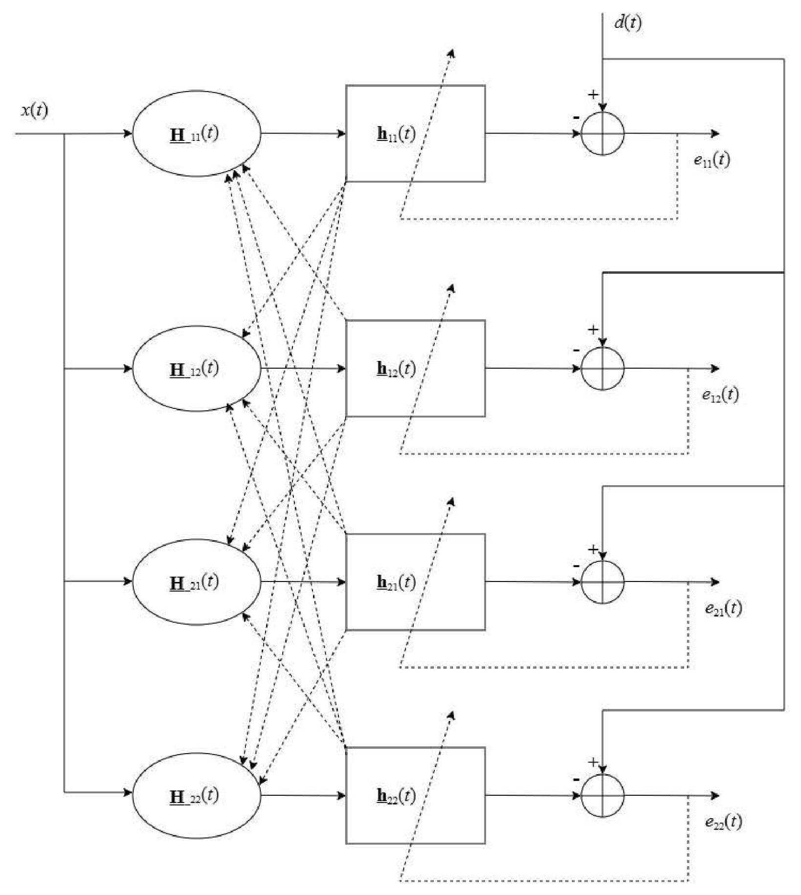
Summarizing, the basic form of the RLS-FOT algorithm is defined by the relations (10), (12), and (17), with 22 , 21 , 12 , 11 . These four component filters are interconnected (via their coefficients) and operate in parallel, as indicated in Figure 1. It can be noticed that the structure of the algorithm is characterized by intrinsic symmetry features.
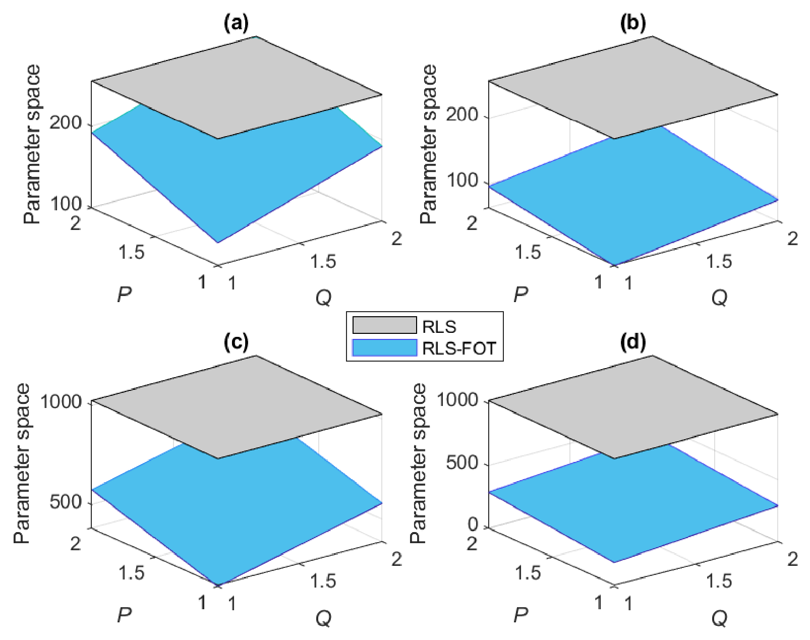
The parameter space of the conventional RLS algorithm comprises L coefficients, which could be problematic for long-length adaptive filters, like in acoustic applications. On the other hand, the RLS-FOT combines four shorter adaptive filters, with a total parameter space of R Q L 22 + R Q L 21 + R P L 12 + R P L 11 coefficients (see Table 1). For the common decomposition setup, there is a significant reduction in the case of the RLS-FOT algorithm, as compared to the conventional approach that considers a single long-length adaptive filter. This is supported in Figure 2, where two examples are examined (for different scenarios), with L = 256 and L = 1024 . In the first case, the factorization is performed using L 11 = L 12 = L 21 = L 22 = 4 , while the second scenario is handled using L 11 = 8 , L 12 = 4 , L 21 = 8 , and L 22 = 4 . As explained in the beginning of this section and also indicated in [36], the common setup for R is in the range L 21 L 22 / 2 to L 21 L 22 / 4 , while the values of P and Q are usually smaller than L 12 / 2 and L 22 / 2 , respectively. Under these circumstances, the parameter space (i.e., the number of coefficients) of the RLS-FOT algorithm is significantly lower than the conventional RLS counterpart, which is represented by the gray surface in Figure 2a–d. Since the computational complexities of these algorithms directly depend on the corresponding number of coefficients, the gain is important in the case of RLS-FOT version, as also supported in [36].

3. RLS-FOT Algorithm with Variable Forgetting Factors

The main control parameters of the RLS-FOT algorithm are the four forgetting factors, i.e., λ 22 , λ 21 , λ 12 , and λ 11 , which correspond to the component filters h ̲ 22 ( t ) , h ̲ 21 ( t ) , h ̲ 12 ( t ) , and h ̲ 11 ( t ) , respectively. The parameters have positive subunitary values, which should be tuned to achieve a proper balance between the tracking capability and the estimate accuracy. Using constant values for the forgetting factors leads to an inherent (yet expected) compromise between these performance criteria. Ideally, large values (i.e., close to one) should be used to obtain a good accuracy of the filter estimate, while smaller values of the forgetting factors improve the tracking behavior. This conflicting requirement can be addressed by using variable forgetting factors (VFFs), which should be designed as time-dependent parameters, i.e., λ 22 ( t ) , λ 21 ( t ) , λ 12 ( t ) , and λ 11 ( t ) . Nevertheless, for practical reasons, the resulting VFFs should be facile to evaluate in real-world/real-time applications, without requiring additional control mechanisms.
To this purpose, we follow the recent idea from [49], which was designed in the framework of the conventional RLS algorithm. First, let us define the a posteriori errors of the RLS-FOT algorithm, which are evaluated similar to (10), but using the updated filters’ coefficients from time index t, i.e.,
e ̲ ( t ) = d ( t ) x ( t ) h ̲ ( t ) ,
with 22 , 21 , 12 , 11 . Since the “input” sequences, x ( t ) , depend on the filters’ coefficients from the previous time index t 1 (see Table 2), the a posteriori errors from (18) are not equal anymore, contrary to the a priori errors from (10). Using the filters’ updates (17) in (18), also considering the a priori errors (10), the relations between these two types of errors result in
e ̲ ( t ) = e ( t ) 1 x ( t ) R 1 ( t ) x ( t ) .
According to (12), the matrix R ( t ) , with 22 , 21 , 12 , 11 , represents an estimate of the covariance matrix of the input sequence x ( t ) . Therefore, based on (12) and considering that t is large enough, we can use the reasonable approximation:
R ( t ) E x ( t ) x ( t ) 1 λ ( t ) ,
where E · denotes the mathematical expectation and the deterministic time-dependent forgetting factors, λ ( t ) ’s, are considered. Also, since the lengths of the corresponding filters are usually much greater than one, the variance of the input sequence x ( t ) , denoted by σ x 2 (with 22 , 21 , 12 , 11 ), can be fairly approximated as the ratio between the product x ( t ) x ( t ) and the corresponding filter length. Under these circumstances, the expressions from (19) become
e ̲ 22 ( t ) e 22 ( t ) 1 R Q L 22 σ x 22 2 1 λ 22 ( t ) E x 22 ( t ) x 22 ( t ) 1 ,
e ̲ 21 ( t ) e 21 ( t ) 1 R Q L 21 σ x 21 2 1 λ 21 ( t ) E x 21 ( t ) x 21 ( t ) 1 ,
e ̲ 12 ( t ) e 12 ( t ) 1 R P L 12 σ x 12 2 1 λ 12 ( t ) E x 12 ( t ) x 12 ( t ) 1 ,
e ̲ 11 ( t ) e 11 ( t ) 1 R P L 11 σ x 11 2 1 λ 11 ( t ) E x 11 ( t ) x 11 ( t ) 1 .
The conventional RLS algorithm results following the LS optimization criterion based on the cost function from (4) [2,3]. It operates on a single filter of length L, using the forgetting factor λ . This control parameter of the RLS filter is usually evaluated as
λ = 1 1 K L ,
with K 1 set as an integer value. The main reason is that λ is a memory-related parameter, which should be associated to the filter length [2,3]. Alternatively, for a better flexibility/control related to the dynamic range of the variables, the forgetting factor can be evaluated as λ = 1 α / L , where α = 1 / K is now limited between 0 and 1. Thus, instead of directly finding a variable forgetting factor, λ ( t ) , the main focus is redirected on designing a time-dependent parameter, α ( t ) . This was the strategy behind the development of the RLS-VFF algorithm from [49]. In the case of RLS-FOT algorithm, the time-dependent forgetting factors should be related to the corresponding filters’ lengths, such that
λ 22 ( t ) = 1 α 22 ( t ) R Q L 22 ,
λ 21 ( t ) = 1 α 21 ( t ) R Q L 21 ,
λ 12 ( t ) = 1 α 12 ( t ) R P L 12 ,
λ 11 ( t ) = 1 α 11 ( t ) R P L 11 ,
where 0 α ( t ) 1 , with 22 , 21 , 12 , 11 . Using (26)–(29) in (21)–(24), we obtain
e ̲ ( t ) e ( t ) 1 σ x 2 α ( t ) E x ( t ) x ( t ) 1 .
At this point, the most problematic terms are the covariance matrices from the right-hand side of (30). An accurate evaluation of these terms represents a difficult task, since the “input” sequences x ( t ) , with 22 , 21 , 12 , 11 , depend on the filters’ coefficients from time index t 1 , as shown in Table 2 and also indicated in Figure 1. Nevertheless, it can be considered that these covariance matrices are still dominated by their main diagonal, so that E x ( t ) x ( t ) σ x 2 I , where I denotes the identity matrix of appropriate size. Clearly, this is a strong assumption, which is especially valid when x ( t ) is white and Gaussian, while the filters’ coefficients are nearly statistically independent. The assumption on the character of the input signal could look quite restrictive, especially in audio applications. However, the motivation behind it is twofold. First, it is used only for deriving the VFFs, while the (full) matrices R ( t ) , with 22 , 21 , 12 , 11 , are still used within the filters’ updates (17). Second, it greatly facilitates the upcoming developments related to the VFFs, since the relations from (30) simplify to
e ̲ ( t ) e ( t ) 1 α ( t ) .
Based on (31), the parameters α ( t ) , with 22 , 21 , 12 , 11 can be obtained by following a natural condition in system identification problems. Let us consider that the reference/desired signal, d ( t ) , is obtained at the output of a system characterized by the impulse response r ( t ) from (1), corrupted by a zero-mean additive noise, v ( t ) , which is uncorrelated to the input signal. Therefore,
d ( t ) = x ( t ) r ( t ) + v ( t ) ,
where x ( t ) is the same input sequence that drives the adaptive filter, like in a system identification scenario [2,3]. In this framework, when the adaptive filter converges to its steady-state, so that h ( t ) r ( t ) , the noise signal should be recovered from the error signal [49,52]. Hence, in the context of RLS-FOT algorithm, the conditions to follow are
E e ̲ 2 ( t ) = σ v 2 ,
with 22 , 21 , 12 , 11 , where σ v 2 is the variance of v ( t ) . Next, squaring and taking the expectations in (31), the set of conditions from (33) leads to the equations:
σ e 2 ( t ) 1 α ( t ) 2 = σ v 2 ,
where σ e 2 ( t ) = E e 2 ( t ) . Considering that α ( t ) ’s are deterministic (with 22 , 21 , 12 , 11 ) and solving the quadratic Equation (34), the valid solutions result in
α ( t ) = 1 σ v σ e ( t ) ,
so that the VFFs from (26)–(29) become
λ 22 ( t ) = 1 1 R Q L 22 1 σ v σ e 22 ( t ) ,
λ 21 ( t ) = 1 1 R Q L 21 1 σ v σ e 21 ( t ) ,
λ 12 ( t ) = 1 1 R P L 12 1 σ v σ e 12 ( t ) ,
λ 11 ( t ) = 1 1 R P L 11 1 σ v σ e 11 ( t ) .
The variances from (36)–(39) can be recursively estimated, using different smoothing factors, i.e.,
σ e 2 ( t ) = a σ e 2 ( t 1 ) + ( 1 a ) e 2 ( t ) ,
σ v 2 ( t ) = b σ v 2 ( t 1 ) + ( 1 b ) e 2 ( t ) ,
where a = 1 1 / L and b = 1 1 / ( β L ) , with β 1 (e.g., on the order of tens). Clearly, different other methods can be used for estimating the noise power; however, the estimation from (41) represents one of the simplest solutions, since it also relies on the error signal, which is already available. As explained after (10), the four a priori errors, e ( t ) , with 22 , 21 , 12 , 11 , are equal to e ( t ) , while the distinct notation is kept for the sake of clarity and the proper association to the corresponding component filters. Thus, the parameters α ( t ) from (35) are also equal, so that the differences between the four VFFs from (36)–(39) are due to the corresponding filters’ lengths. Since the VFFs involve the estimation of σ v 2 , which is associated to the external additive noise, a challenging situation could appear when v ( t ) is nonstationary, as in the double-talk case [1]. In such a scenario, two approaches can be considered: (i) a double-talk detector to control the algorithm behavior during that period and (ii) a more rigorous estimation of σ v 2 ( t ) , which will be subject for future works. While the estimation from (41) is one of the simplest and most practical solutions, it might not cope with the double-talk scenario, where the nonstationary nature of the near-end speech could significantly bias the adaptive filter behavior. In this context, a regularized version of the algorithm could also be considered in perspective, by incorporating proper regularization terms within the cost functions from (5)–(8), aiming to improve the overall robustness against different external perturbations.
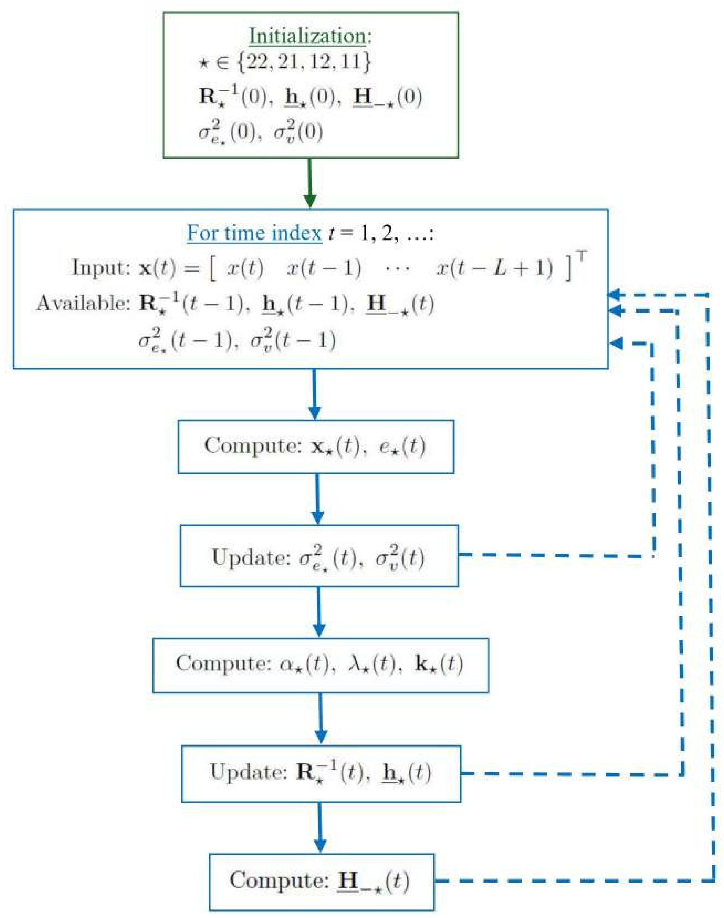
The resulting RLS-FOT algorithm with VFFs has been formulated following the basic form of the algorithm from Section 2, which facilitated the previous development. Nevertheless, the designed VFFs can be incorporated within the RLS-FOT version from [36], which uses the matrix inversion lemma to avoid the direct evaluation of R 1 ( t ) from (17). In this context, the proposed algorithm (referred as RLS-FOT-VFFs) is summarized in Table 3. Here, the notation I and 0 indicate the identity matrix and an all-zeros column vector, respectively, with the corresponding size/length indicated in subscript. In addition, a flowchart of the algorithm is depicted in Figure 3.
The initialization for R 1 ( 0 ) , with 22 , 21 , 12 , 11 , requires the positive constant γ on the main diagonal, in order to prevent potential numerical issues. This is a standard initialization of the RLS-type algorithms, which represents the simplest and most practical solution. Other more rigorous initialization procedures could be considered, as indicated in [53]. Nevertheless, due to the presence of the subunitary forgetting factors, λ ( t ) , the contribution of the initialization of R 1 ( 0 ) is quickly attenuated through the iterations and has basically no influence in the steady-state of the algorithm. Usually, the all-zeros initialization is used for the coefficients of the adaptive filter. However, due to the combination that involves the Kronecker products (see also Table 2), the all-zeros initialization would stall the RLS-FOT-VFFs algorithm. Consequently, the small positive constant ε 1 is used to prevent this issue, as shown in Table 3. Finally, a very small positive constant, ϵ 1 , is added to the denominator of α ( t ) , with 22 , 21 , 12 , 11 , in order to avoid divisions by zero.
Due to the use of the matrix inversion lemma to update the matrices R 1 ( t ) , with 22 , 21 , 12 , 11 , the notation for the Kalman gain vectors [2,3] is used in Table 3, i.e., k ( t ) . This allows a more compact expression for the update of R 1 ( t ) , but also for the coefficients’ update, h ̲ ( t ) . Clearly, the filters’ updates from (17) are equivalent to the updates of h ̲ ( t ) from Table 3, since k ( t ) = R 1 ( t ) x ( t ) .
The computational complexity of the proposed RLS-FOT-VFFs algorithm is on the same order with its RLS-FOT counterpart from [36]. The specific operations of the RLS-FOT-VFFs algorithm are related to the evaluation of its time-dependent forgetting factors, i.e., the computation of σ e 2 ( t ) , σ v 2 ( t ) , α ( t ) , and λ ( t ) , with 22 , 21 , 12 , 11 . These require only a few extra operations, with a total amount of 5 × 4 = 20 multiplications, 5 × 4 = 20 additions, 2 × 4 = 8 divisions, and 2 × 4 = 8 square-roots operations, for all the four component filters. As indicated in [36], the complexity order of the RLS-FOT algorithm is O ( R Q L 22 ) 2 + ( R Q L 21 ) 2 + ( R P L 12 ) 2 + ( R P L 11 ) 2 , so that the extra computational amount required by the VFFs’ evaluation is negligible and does not depend on the filters’ lengths.
A detailed evaluation of the computational complexities (in terms of the number of multiplications and additions per iteration) of the main comparing algorithms is included in Table 4. Here, the computational amounts that mainly involve Kronecker product operations and lead to x ( t ) (see Table 2) are denoted by O × and O + , respectively. Generally, these amounts are on the order of 4 R Q P L , even if the specific operations related to the Kronecker product can be further optimized [54,55]. As a numerical example, let us consider the length L = 1024 , which is factorized using L 11 = 8 , L 12 = 4 , L 21 = 8 , and L 22 = 4 . In this case, the conventional RLS algorithm and the RLS-VFF version from [49] require around 2.1 × 10 6 multiplications and 2.099 × 10 6 additions (per iteration). On the other hand, the decomposition-based algorithms, i.e., RLS-FOT [36] and RLS-FOT-VFFs (both using R = L 21 L 22 / 2 , P = L 12 / 2 , and Q = L 22 / 2 ) need around 0.591 × 10 6 multiplications and 0.590 × 10 6 additions (per iteration). Here, the decomposition parameters R, P, and Q have been set to their maximum recommended values (as explained in the beginning of Section 2), so that the resulting computational amount represents an upper bound. Using smaller values for these parameters (as also supported in the next section), significantly reduce the computational complexity of the decomposition-based algorithms.

4. Simulation Results

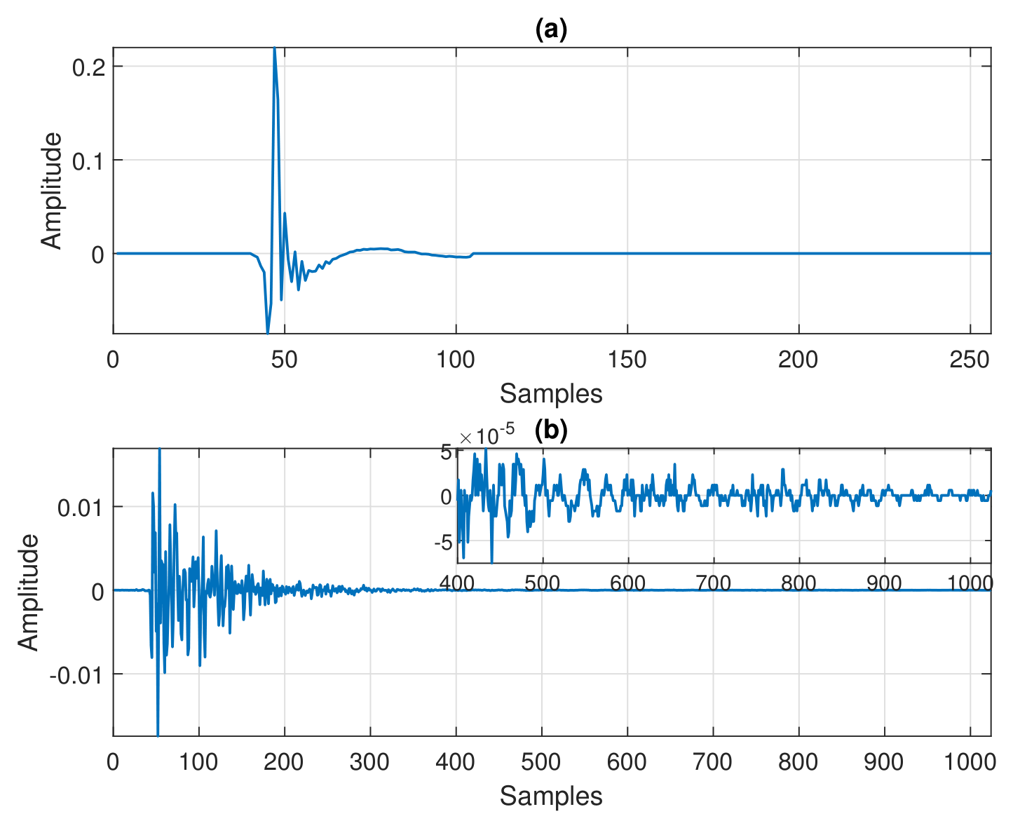
The performances of the proposed RLS-FOT-VFFs algorithm are assessed in the framework of echo cancellation [1,56]. Two impulse responses are considered in the experiments, as shown in Figure 4a,b, with the lengths L = 256 and L = 1024 , respectively; the sampling rate is 8 kHz. The first one is a network impulse response from ITU-T G168 Recommendation [56], which is obtained using the first cluster of coefficients padded with zeros up to the length L = 256 . The second one is a measured acoustic impulse response of length L = 1024 . The factorization of L = 256 is performed using L 11 = L 12 = L 21 = L 22 = 4 , while L = 1024 is factorized with L 11 = 8 , L 12 = 4 , L 21 = 8 , and L 22 = 4 , respectively. Different other factorization strategies can be used, as discussed in [36]. However, the main goal of the current experiments is to support the performance features of the VFFs-based approach. These impulse responses are selected to illustrate the behavior for both sparse and dispersive systems, which can be associated to network and acoustic echo cancellation, respectively. Their different lengths allow a twofold evaluation, i.e., (i) related to the FOT factorization and (ii) related to the influence of the length of the adaptive filter.
The input sequence is a noisy speech obtained from different recorded female voices available in the Open Speech Repository [57], which are selected among the first 10 files from the “American English” category. Nevertheless, the performances of the algorithms are very similar when using different speech sequences. The input signal represents the voice of the far-end speaker, x ( t ) , which propagates through the echo path, r ( t ) , thus resulting the echo signal. Further, the echo signal is corrupted by a background noise, v ( t ) , thus obtaining the reference/desired signal, d ( t ) , from (32). In this context, the signal-to-noise ratio (SNR) is defined as the ratio between the variance of the echo signal and σ v 2 . Its value is set to 20 dB in most of the experiments, which represents a realistic communication scenario, with moderate SNR. Also, in some simulations, a noisy environment is considered, using SNR = 10 dB. The tracking capabilities of the adaptive filter are assessed in each experiment, by abruptly changing the echo path, introducing a right-shift of its impulse response by 8 samples.
Since echo cancellation basically represents a system identification problem, where the adaptive filter, h ( t ) , is used to model/estimate the impulse response of the echo path, r ( t ) , a standard performance measure is the normalized misalignment (or system mismatch) [1]. This is defined (in dB) as 20 log 10 r ( t ) h ( t ) / r ( t ) , where · denotes the Euclidean norm. Clearly, a lower misalignment indicates a better accuracy of the algorithm. Also, a steeper misalignment curve indicates a better convergence rate and/or tracking capability of the adaptive filter.
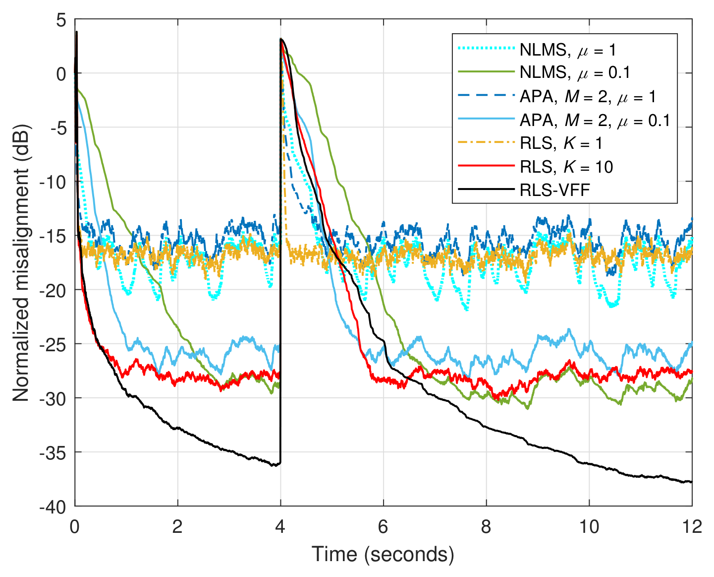
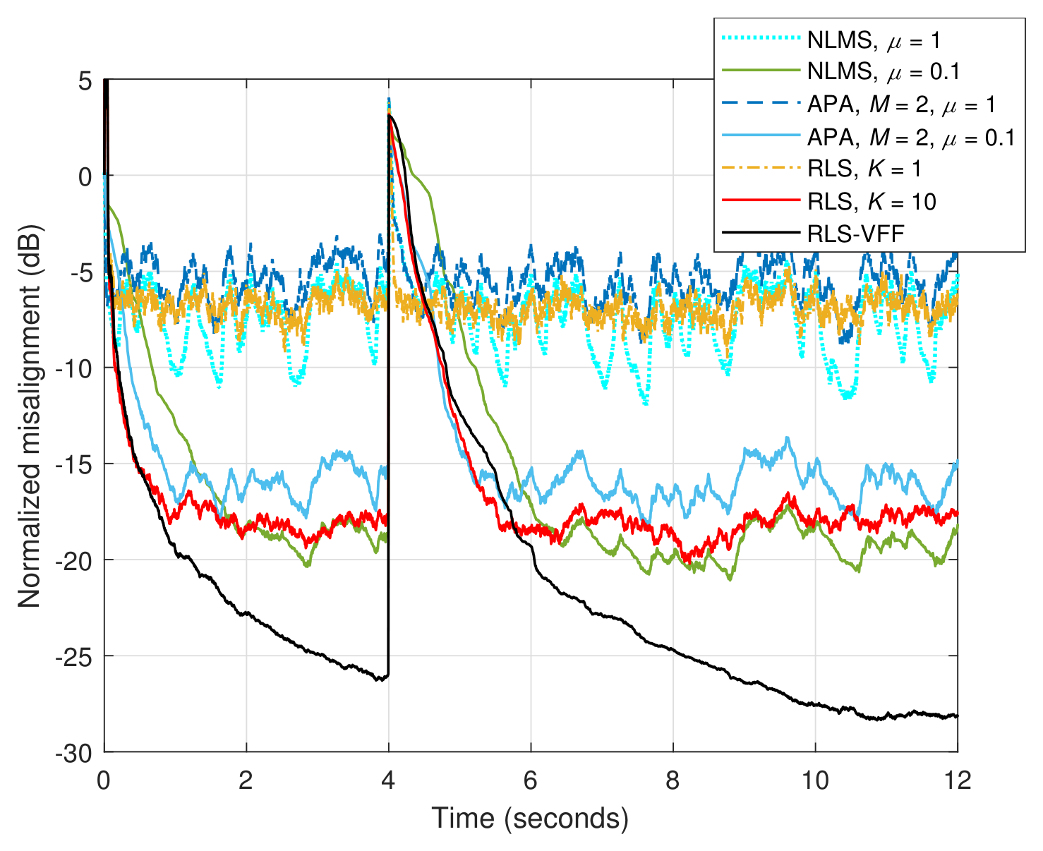
In order to establish the benchmarks used in comparisons, a preliminary set of experiments evaluates the performances of several standard algorithms, as compared to the recently developed RLS-VFF version from [49], for the identification of the impulse response from Figure 4a. In terms of computational complexity and facility of implementation, the normalized least-mean-square (NLMS) algorithm is usually considered the workhorse in adaptive filtering [2,3], with a computational complexity proportional to O ( L ) . Its main control parameter is the normalized step-size, μ , which is a positive constant smaller than 2 (for stability), with the fastest convergence mode obtained for μ = 1 . On the other hand, a fast convergence rate is paid by a reduced accuracy of the filter estimate (i.e., larger misalignment). Besides, the NLMS algorithm is sensitive to the character of the input data, especially in terms of the correlation degree. To overcome this shortcoming, the affine projection algorithm (APA) [58] represents an appealing alternative, with better convergence properties for correlated inputs and a moderate increase of the computational complexity, as compared to the NLMS algorithm. Besides the step-size parameter, the performance of APA is influenced by the projection order, M, which is a positive integer larger than or equal to one. In fact, for M = 1 , the APA is equivalent to the NLMS algorithm. When the value of M increases, the convergence rate of APA is improved, especially for correlated inputs. The computational complexity of APA is proportional to O ( M L ) , so that it is proportional to the filter length. On the other hand, the standard RLS algorithm requires a computational amount proportional to O ( L 2 ) , while owning improved convergence properties as compared to APA, even for correlated inputs. Its performance is controlled by the forgetting factor, which is usually set based on (25).
The performances of these standard algorithms are shown in Figure 5 and Figure 6, for SNR = 20 dB and 10 dB, respectively. Different values of the specific convergence parameters are set for the standard algorithms, outlining their influence on the overall behavior. As explained before, μ = 1 leads to the fastest convergence/tracking of NLMS/APA, but with a high misalignment level. On the other hand, a smaller value of μ improves the accuracy (i.e., lower misalignment), but pays with a slower convergence/tracking. The influence of the projection order of APA is also revealed in Figure 5 and Figure 6, improving the convergence rate and tracking of the NLMS algorithm, while reaching a higher misalignment level. The RLS algorithm obtains the fastest initial convergence rate, but its tracking capability is highly influenced by the value of the forgetting factor. For example, a larger value of λ (or K) leads to a better accuracy of the filter estimate (i.e., lower misalignment), while paying with a slower tracking reaction. In this context, the RLS-VFF algorithm from [49] outperforms its standard counterparts, achieving a better balance between the main performance criteria, with fast convergence/tracking and low misalignment. The same conclusions are valid for different SNR levels.
As a result, the selection of the comparing algorithms is made based on the following considerations. First, as indicated in [36], the RLS-FOT algorithm can outperform other previously developed decomposition-based counterparts [7,34], so that it is considered as a comparison benchmark. It uses the same decomposition setup as the proposed VFFs-based algorithm, while its forgetting factors are set as constant values, following the rule-of-thumb mentioned in Section 3. Hence, the settings are
λ = 1 1 K L ,
with 22 , 21 , 12 , 11 and K > 1 , while L generally denotes the length of the corresponding component filter, i.e., R Q L 22 , R Q L 21 , R P L 12 , and R P L 11 , respectively. Second, supported by the previous set of experiments, the RLS-VFF algorithm from [49] is considered in comparisons, which relies on a similar idea for developing its time-dependent forgetting factor. In this case, its VFF is evaluated as
λ ( t ) = 1 α ( t ) L ,
with α ( t ) = 1 σ v ( t ) / σ e ( t ) , where the variances are evaluated similar to (40) and (41). As indicated in [49], this algorithm outperforms the conventional RLS benchmark (see also Figure 5 and Figure 6) and other VFF-based RLS-type algorithms. Nevertheless, it involves a single (long-length) adaptive filter, with L coefficients, which inherently influences its performance features. On the other hand, the proposed RLS-FOT-VFFs algorithm combines the estimates provided by four (much) shorter adaptive filters, with expected gains in terms of tracking and accuracy.
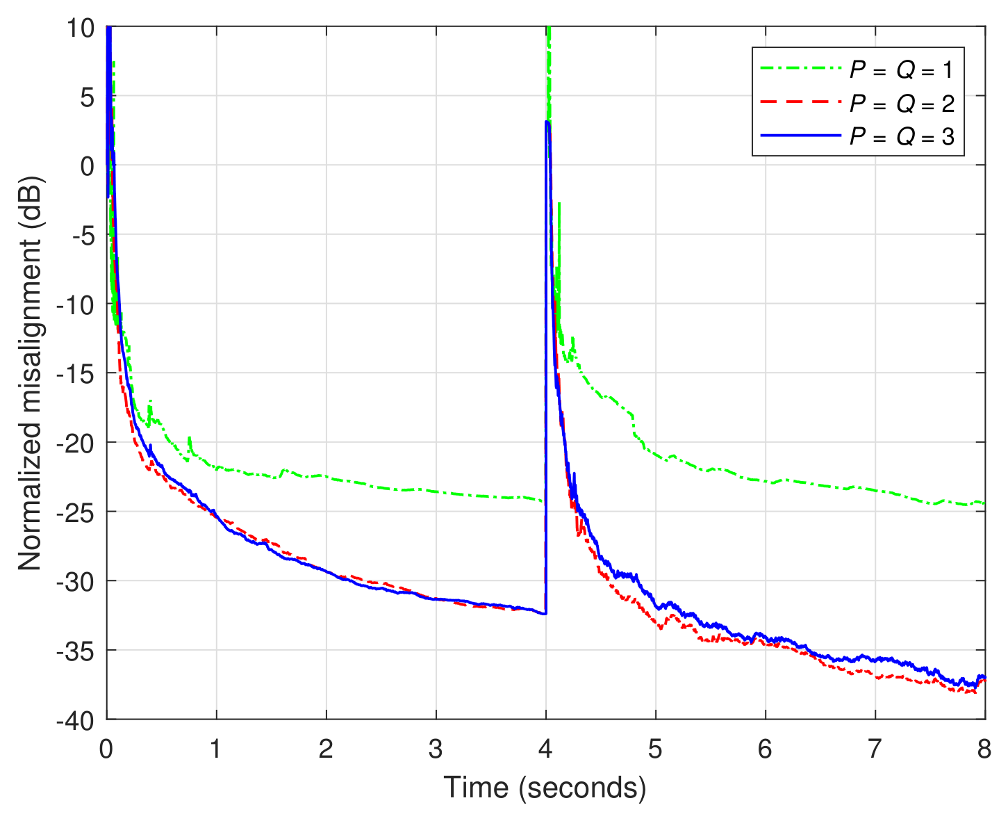
In the first set of experiments, the identification of the sparser impulse response ( L = 256 ) from Figure 4a is evaluated. Figure 7 shows the results obtained by the RLS-FOT-VFFs algorithm for different values of P = Q , using R = L 12 L 22 / 2 = 8 and β = 20 in (41). It can be noticed that even for P = Q = 1 , the proposed algorithm obtains a misalignment level around 25 dB, which represents a good balance between performance and complexity. As expected, the performance is improved for P = Q = 2 , these values being equivalent to L 12 / 2 and L 22 / 2 , respectively. Increasing the values of P and Q beyond these limits is not justified in terms of performance improvement, as also noticed in Figure 7.
Next, the influence of the decomposition parameter R is investigated in Figure 8. This parameter is related to the first “level” of the NKP decomposition, according to (1). Usually, as also indicated in previous works [36], this value does not exceed L 12 L 22 / 2 for low-rank impulse responses. In this context, the values considered in Figure 8 are R = 4 = L 12 L 22 / 4 , R = 6 L 12 L 22 / 3 , and R = 8 = L 12 L 22 / 2 . Clearly, the performance is improved (i.e., lower misalignment) for larger values of R, while there is an inherent saturation at some point. Taking into account that the computational complexity also increases with the value of R, the practical limit R = L 12 L 22 / 2 could be considered as a recommended choice.
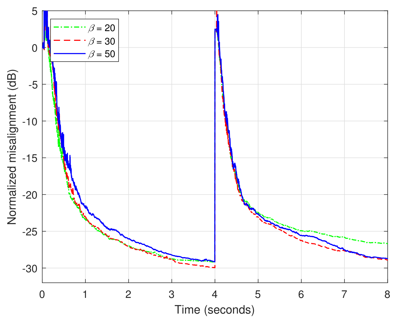
The only parameter that has to be set within the RLS-FOT-VFFs algorithm from Table 3 is related to the smoothing factor used within the estimation of σ v 2 ( t ) from (41). As indicated in Section 3, the value of β should be much larger than one, e.g., on the order of tens. In Figure 9, the influence of β on the overall performance of the RLS-FOT-VFFs algorithm is not very relevant, especially in terms of tracking. Therefore, a value in the vicinity of β = 20 or β = 30 could represent a practical setting. This is also in consistence with the results reported in [49], for the RLS-VFF counterpart.
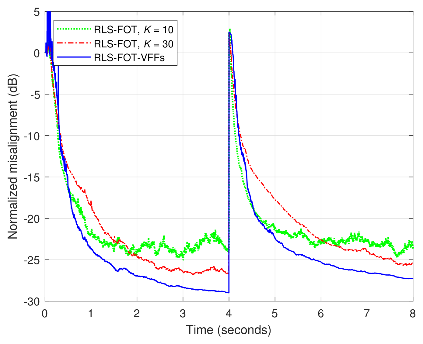
The next experiment from this first set is dedicated to the comparison with the RLS-FOT algorithm from [36] and the RLS-VFF filter from [49]. As explained before, these two algorithms represent recent benchmarks for the decomposition-based versions, respectively for the VFF-based counterparts. In Figure 10, the RLS-FOT algorithm [36] uses the same decomposition setup as the proposed RLS-FOT-VFFs (i.e., P = Q = 2 and R = L 12 L 22 / 2 ), while different values of the forgetting factors are used, by setting the parameter K in (42). Also, the RLS-VFF algorithm [49] uses the same β = 20 as the proposed RLS-FOT-VFFs, while its (single) forgetting factor is evaluated as in (43), considering a single (long-length) filter with L coefficients. Since the RLS-FOT-VFFs algorithm operates with shorter adaptive filters, its tracking capability is significantly better, as compared to the RLS-VFF benchmark. Also, the proposed version reaches a lower misalignment level (i.e., a better accuracy of the estimate), as compared to the RLS-FOT counterpart, which uses constant forgetting factors. In order to improve the accuracy of the RLS-FOT algorithm, its forgetting factors should be increased (e.g., by increasing the value of K), while paying in terms of the tracking behavior. Overall, the proposed RLS-FOT-VFFs algorithm obtains a better balance in terms of these performance criteria.
The advantages of the decomposition-based algorithm are also valid for different SNR conditions. As an example, in Figure 11, the proposed RLS-FOT-VFFs algorithm is compared to the RLS-VFF counterpart from [49], under a noisy scenario, with SNR = 10 dB. Both algorithms achieve a similar accuracy at steady-state (i.e., a similar misalignment level), while the FOT-based algorithm has a better tracking reaction, due to the combination of shorter adaptive filters.
In the second set of experiments, the longer (and less sparse) acoustic impulse response from Figure 4b is considered, with the length L = 1024 . First, the influence of the decomposition parameters P and Q is assessed in Figure 12, while using R = L 21 L 22 / 2 . Here, the RLS-VFF algorithm from [49] is considered as a comparison benchmark. Both algorithms use β = 20 for the estimation of σ v 2 ( t ) from (41). It can be noticed that the proposed RLS-FOT-VFFs algorithm has a significantly better tracking capability, as compared to the RLS-VFF counterpart, since the decomposition-based version combines shorter adaptive filters. In terms of misalignment (i.e., accuracy), the performance of the RLS-FOT-VFFs algorithm is improved for P = Q = 2 (which corresponds to L 12 / 2 = L 22 / 2 = 2 ) , as compared to the case when P = Q = 1 . Nevertheless, even when using the smallest values of P and Q (i.e., the lowest complexity), the proposed algorithm reaches a misalignment level below 20 dB, while still outperforming the RLS-VFF version [49] in terms of the tracking capability.
Related to this experiment, the time-dependent forgetting factors of the RLS-VFF and RLS-FOT-VFFs algorithms are depicted in Figure 13. In the case of RLS-VFF algorithm [49], its forgetting factor is evaluated based on (43) and it operates on a single (long-length) filter with L = 1024 coefficients. The forgetting factors of the proposed RLS-FOT-VFFs algorithm (with R = L 21 L 22 / 2 and P = Q = 2 ) are evaluated based on (36)–(39). Due to the decomposition settings from Figure 12, it results that λ 11 ( t ) = λ 21 ( t ) , which correspond to two of the component filters, with the lengths R P L 11 = R Q L 21 = 256 . Also, we have λ 12 ( t ) = λ 22 ( t ) , related to the other two component filters, having the lengths R P L 12 = R Q L 22 = 128 . The faster tracking capability of the RLS-FOT-VFFs algorithm can be assessed from Figure 13b,c, due to the evolution of its VFFs, as compared to the behavior of the RLS-VFF algorithm [49] from Figure 13a, where λ ( t ) has a slower tracking reaction.
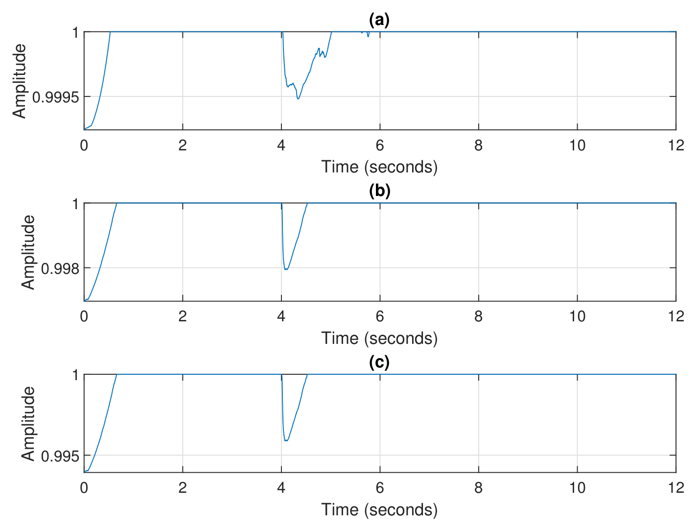
The previous experiment related to Figure 12 and Figure 13 is reconsidered under a noisy scenario, with SNR = 10 dB, and the results are shown in Figure 14 and Figure 15, respectively. As we can notice in Figure 14, the proposed RLS-FOT-VFFs algorithm (using P = Q = 2 and R = L 21 L 22 / 2 ) clearly outperforms the RLS-VFF counterpart from [49] in terms of the tracking capability, while reaching a similar misalignment level at steady-state. This behavior is also supported in Figure 15, by the evolution of the time-dependent forgetting factors corresponding to the comparing algorithms.
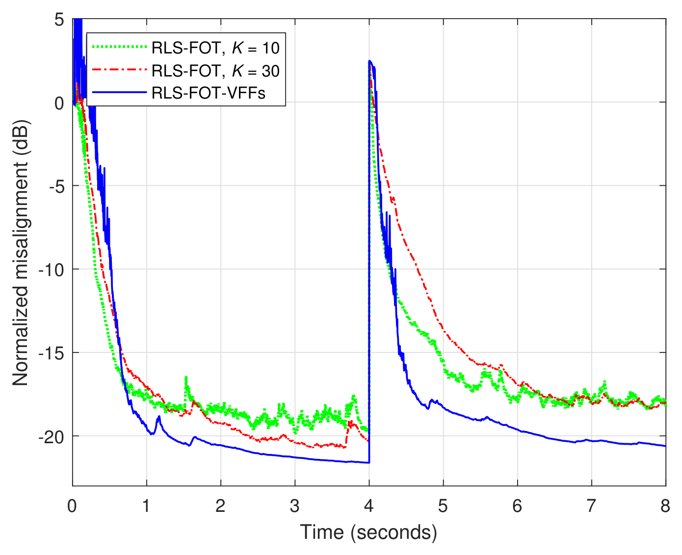
The main feature of the proposed RLS-FOT-VFFs algorithm, as compared to the recently developed RLS-FOT version from [36], consists in a better balance between the main performance criteria, i.e., accuracy versus tracking. This is supported in Figure 16, where both algorithms involve the same decomposition setup (with P = Q = 2 and R = L 21 L 22 / 2 ), while the RLS-FOT algorithm [36] uses different constant forgetting factors, by tuning the value of K in (42). As expected, larger values of the forgetting factors (i.e., a larger value of K) improve the accuracy of the RLS-FOT algorithm, with the cost of a slower tracking reaction. Reducing the value of K results in using smaller values of the forgetting factors, which improve the tracking behavior, but paying with a higher misalignment level. Overall, it can be noticed that the RLS-FOT-VFFs algorithm achieves a better compromise between these performance features.
A similar conclusion can be reached when using a smaller value of the decomposition parameter R, which corresponds to a lower computational complexity. In Figure 17, the previous experiment is repeated, but using R = L 21 L 22 / 4 . The results outline the same advantageous behavior of the proposed RLS-FOT-VFFs algorithm, in terms of its better performance balance, obtaining a good misalignment level (below 20 dB), together with a fast tracking reaction.
Finally, the influence of the smoothing factor used for the estimation of σ v 2 ( t ) from (41) is assessed. In Figure 18, different values of β (on the order of tens) are considered, while the decomposition settings of the RLS-FOT-VFFs algorithm are P = Q = 2 and R = L 21 L 22 / 2 . It can be noticed that the proposed algorithm is fairly robust to the selection of β , which is the only parameter to be set related to the VFFs’ part of the filter. This also represents a practical asset of the RLS-FOT-VFFs algorithm.


5. Conclusions and Perspectives

In the current paper, the RLS-FOT-VFFs algorithm has been proposed, by following the recently developed RLS-FOT algorithm [36] and designing time-dependent forgetting factors (i.e., VFFs) as the main control parameters. The FOT-based approach can be interpreted as a “double-level” NKP decomposition, which leads to a combination of four (shorter) adaptive filters working in parallel, with intrinsic symmetry features. This technique fits very well for the identification of low-rank long-length impulse responses (i.e., with hundreds/thousands of coefficients), like in echo cancellation. Thus, instead of using a single (long-length) RLS adaptive filter, as in the conventional approach, the RLS-FOT algorithms exploit this efficient fourth-order decomposition and gain in terms of both performance and complexity. The idea behind the VFFs of the proposed algorithm is inspired by the recent work from [49], where a practical RLS-VFF algorithm was designed. A specific characteristic of the RLS-FOT-VFFs algorithm is that it operates with four individual forgetting factors, which depend on the lengths of the corresponding component filters.
The proposed RLS-FOT-VFFs algorithm inherits the advantages of the decomposition-based technique (i.e., the combination of shorter filters), but also the convergence/tracking features related to its time-dependent control parameters, which lead to an improved balance between the main performance criteria (e.g., accuracy versus tracking). As a result, it outperforms the RLS-FOT algorithm from [36], which operates with constant values of the forgetting factors, but also the RLS-VFF version from [49], which handles a single long-length adaptive filter. Simulation results obtained in the framework of echo cancellation support these performance gains.
The basic goal of the current work was to outline the main performance features of the RLS-FOT-VFFs algorithm. In perspective, several directions for future research could be followed. First, alternative methods for solving the normal equations of the algorithm could be considered. For example, the QRD-based approach [59] represents an appealing alternative, in terms of both complexity and stability. Besides, the dichotomous coordinate descent (DCD) iterative methods [60,61,62,63,64] are recognized as popular solutions for efficient hardware implementations. Second, more elaborate methods for estimating the noise power (required within the VFFs) could be explored, targeting a robust behavior of the algorithm in different challenging scenarios, like double-talk (in echo cancellation) [1]. In this context, exploiting the VFFs-based version while using regularized-type LS cost functions could also represent a promising solution for improved robustness. Finally, more realistic experimental scenarios will be considered, including real acoustic environments, with different types of noise/interference that can be present in practical communication systems [65]. In this framework, the double-talk case also represents a challenging situation for real-world AEC systems, which has to be considered in practical implementations.

Author Contributions

Conceptualization, R.-A.O.; methodology, C.-L.S.; investigation, C.P.; validation, J.B.; software, L.-M.D.; formal analysis, R.-L.C. All authors have read and agreed to the published version of the manuscript.

Funding

This research received no external funding.

Data Availability Statement

The original contributions presented in this study are included in the article. Further inquiries can be directed to the corresponding author.

Conflicts of Interest

The authors declare no conflict of interest.

References

  1. Hänsler, E.; Schmidt, G. Acoustic Echo and Noise Control–A Practical Approach; Wiley: Hoboken, NJ, USA, 2004. [Google Scholar]
  2. Haykin, S. Adaptive Filter Theory, 5th ed.; Pearson: Upper Saddle River, NJ, USA, 2014. [Google Scholar]
  3. Diniz, P.S.R. Adaptive Filtering: Algorithms and Practical Implementation, 5th ed.; Springer Nature: Cham, Switzerland, 2020. [Google Scholar]
  4. Söderstrxoxm, T.; Stoica, P. System Identifcation; Prentice-Hall International: Hertfordshire, UK, 1989. [Google Scholar]
  5. Ljung, L. System Identification: Theory for the User, 2nd ed.; Prentice-Hall: Upper Saddle River, NJ, USA, 1999. [Google Scholar]
  6. Paleologu, C.; Benesty, J.; Ciochină, S. Linear system identification based on a Kronecker product decomposition. IEEE/ACM Trans. Audio Speech Lang. Process. 2018, 26, 1793–1808. [Google Scholar]
  7. Elisei-Iliescu, C.; Paleologu, C.; Benesty, J.; Stanciu, C.; Anghel, C.; Ciochină, S. Recursive least-squares algorithms for the identification of low-rank systems. IEEE/ACM Trans. Audio Speech Lang. Process. 2019, 27, 903–918. [Google Scholar]
  8. Dogariu, L.M.; Benesty, J.; Paleologu, C.; Ciochină, S. Identification of room acoustic impulse responses via Kronecker product decompositions. IEEE/ACM Trans. Audio Speech Lang. Process. 2022, 30, 2828–2841. [Google Scholar]
  9. Bhattacharjee, S.S.; George, N.V. Nearest Kronecker product decomposition based normalized least mean square algorithm. In Proceedings of the IEEE International Conference on Acoustics, Speech, and Signal Processing (ICASSP), Barcelona, Spain, 4–8 May 2020; pp. 476–480. [Google Scholar]
  10. Bhattacharjee, S.S.; George, N.V. Fast and efficient acoustic feedback cancellation based on low rank approximation. Signal Process. 2021, 182, 107984. [Google Scholar] [CrossRef] [Scilit]
  11. Bhattacharjee, S.S.; George, N.V. Nearest Kronecker product decomposition based linear-in-the-parameters nonlinear filters. IEEE/ACM Trans. Audio Speech Lang. Process. 2021, 29, 2111–2122. [Google Scholar]
  12. Bhattacharjee, S.S.; Patel, V.; George, N.V. Nonlinear spline adaptive filters based on a low rank approximation. Signal Process. 2022, 201, 108726. [Google Scholar] [CrossRef] [Scilit]
  13. Vadhvana, S.; Yadav, S.K.; Bhattacharjee, S.S.; George, N.V. An improved constrained LMS algorithm for fast adaptive beamforming based on a low rank approximation. IEEE Trans. Circuits Syst. II Express Briefs 2022, 69, 3605–3609. [Google Scholar]
  14. Dehghan, M.; Goulart, J.H.; de Almeida, A.L.F. Low-rank multilinear filtering. Digit. Signal Process. 2024, 153, 104646. [Google Scholar] [CrossRef] [Scilit]
  15. Ye, J.; Zhao, H. Nearest Kronecker product decomposition based subband adaptive filter: Algorithms and applications. IEEE Trans. Audio Speech Lang. Process. 2026, 34, 691–706. [Google Scholar] [CrossRef] [Scilit]
  16. Frank, J.S.A.; Cohen, I.; George, N.V. Generalized sidelobe canceller for time-domain region-of-interest beamforming. IEEE Trans. Audio Speech Lang. Process. 2026, 34, 878–894. [Google Scholar]
  17. Ghosh, S.; Meena, T.; George, N.V. Low-rank enhanced Hammerstein-spline adaptive filter for sparsity-aware nonlinear feedback cancellation in hearing aids. Signal Process. 2026, 244, 110518. [Google Scholar]
  18. Wang, X.; Yan, G. Sparse diffusion Kronecker-RLS for adaptive learning in wireless sensor networks. Circuits Syst. Signal Process. 2026. early access. [Google Scholar]
  19. Li, L.; Cui, M.; Liu, X.; Zheng, Y.; Wang, S.; Jensen, J.R.; Christensen, M.G. Two-layer Kronecker product decomposition-based robust recursive adaptive filtering for multichannel active noise control. Mech. Syst. Signal Process. 2026, 249, 114053. [Google Scholar]
  20. Ye, J.; Zhao, H.; Lv, S.; Zhou, Y. Fractional-order subband p-norm adaptive filter via transformation nearest Kronecker product decomposition for active noise control. Mech. Syst. Signal Process. 2026, 249, 114073. [Google Scholar]
  21. Vargas, D.; Avalos, J.G.; Vázquez, Á.A.; Sxaxnchez, G.; Vxaxzquez, E.; Avalos, G. A Kronecker product RSOR algorithm applied to acoustic echo cancellation. IEEE Embed. Syst. Lett. 2026. early access. [Google Scholar]
  22. Golub, G.H.; Loan, C.F.V. Matrix Computations, 3rd ed.; The John Hopkins University Press: Baltimore, MD, USA, 1996. [Google Scholar]
  23. Hansen, P.C. Rank-Deficient and Discrete Ill-Posed Problems: Numerical Aspects of Linear Inversion; SIAM: Philadelphia, PA, USA, 1998. [Google Scholar]
  24. Kolda, T.G.; Bader, B.W. Tensor decompositions and applications. SIAM Rev. 2009, 51, 455–500. [Google Scholar] [CrossRef] [Scilit]
  25. Salmi, J.; Richter, A.; Koivunen, V. Sequential unfolding SVD for tensors with applications in array signal processing. IEEE Trans. Signal Process. 2009, 57, 4719–4733. [Google Scholar] [CrossRef] [Scilit]
  26. Comon, P. Tensors: A brief introduction. IEEE Signal Process. Mag. 2014, 31, 44–53. [Google Scholar] [CrossRef] [Scilit]
  27. Vervliet, N.; Debals, O.; Sorber, L.; Lathauwer, L.D. Breaking the curse of dimensionality using decompositions of incomplete tensors: Tensor-based scientific computing in big data analysis. IEEE Signal Process. Mag. 2014, 31, 71–79. [Google Scholar] [CrossRef] [Scilit]
  28. Friedland, S.; Tammali, V. Low-rank approximation of tensors. In Numerical Algebra, Matrix Theory, Differential-Algebraic Equations and Control Theory; Benner, P., Bollhöfer, M., Kressner, D., Mehl, C., Stykel, T., Eds.; Springer: Cham, Switzerland, 2015; pp. 377–411. [Google Scholar]
  29. Cichocki, A.; Mandic, D.P.; Phan, A.; Caiafa, C.F.; Zhou, G.; Zhao, Q.; Lathauwer, L.D. Tensor decompositions for signal processing applications: From two-way to multiway component analysis. IEEE Signal Process. Mag. 2015, 32, 145–163. [Google Scholar] [CrossRef] [Scilit]
  30. Becker, H.; Albera, L.; Comon, P.; Gribonval, R.; Wendling, F.; Merlet, I. Brain-source imaging: From sparse to tensor models. IEEE Signal Process. Mag. 2015, 32, 100–112. [Google Scholar] [CrossRef] [Scilit]
  31. Bousse, M.; Debals, O.; Lathauwer, L.D. A tensor-based method for large-scale blind source separation using segmentation. IEEE Trans. Signal Process. 2017, 65, 346–358. [Google Scholar]
  32. Sidiropoulos, N.; Lathauwer, L.D.; Fu, X.; Huang, K.; Papalexakis, E.; Faloutsos, C. Tensor decomposition for signal processing and machine learning. IEEE Trans. Signal Process. 2017, 65, 3551–3582. [Google Scholar] [CrossRef] [Scilit]
  33. Benesty, J.; Paleologu, C.; Ciochină, S. Linear system identification based on a third-order tensor decomposition. IEEE Signal Process. Lett. 2023, 30, 503–507. [Google Scholar] [CrossRef] [Scilit]
  34. Paleologu, C.; Benesty, J.; Stanciu, C.L.; Jensen, J.R.; Christensen, M.G.; Ciochină, S. Recursive least-squares algorithm based on a third-order tensor decomposition for low-rank system identification. Signal Process. 2023, 213, 109216. [Google Scholar]
  35. Benesty, J.; Paleologu, C.; Dogariu, L.M. An iterative Wiener filter based on a fourth-order tensor decomposition. Symmetry 2023, 15, 1560. [Google Scholar] [CrossRef] [Scilit]
  36. Otopeleanu, R.A.; Dogariu, L.M.; Paleologu, C.; Benesty, J.; Stanciu, C.L.; Costea, R.L. Recursive least-squares algorithm based on a fourth-order tensor decomposition for acoustic echo cancellation. Mathematics 2026, 14, 812. [Google Scholar]
  37. Chan, S.-C.; Tan, H.-J.; Lin, J.-Q.; Liao, B. A new local polynomial modeling based variable forgetting factor and variable regularized PAST algorithm for subspace tracking. IEEE Trans. Aerosp. Electron. Syst. 2018, 54, 1530–1544. [Google Scholar] [CrossRef] [Scilit]
  38. Song, Q.; Mi, Y.; Lai, W. A novel variable forgetting factor recursive least square algorithm to improve the anti-interference ability of battery model parameters identification. IEEE Access 2019, 7, 61548–61557. [Google Scholar] [CrossRef] [Scilit]
  39. Tan, H.J.; Chan, S.C.; Lin, J.Q.; Sun, X. A new variable forgetting factor-based bias-compensated RLS algorithm for identification of FIR systems with input noise and its hardware implementation. IEEE Trans. Circuits Syst. I Regul. Pap. 2020, 67, 198–211. [Google Scholar]
  40. Lin, J.-Q.; Wu, H.-C.; Chan, S.-C. A new regularized recursive dynamic factor analysis with variable forgetting factor and subspace dimension for wireless sensor networks with missing data. IEEE Trans. Instrum. Meas. 2021, 70, 1–13. [Google Scholar] [CrossRef] [Scilit]
  41. Yu, Y.; Lu, L.; Zakharov, Y.; de Lamare, R.C.; Chen, B. Robust sparsity-aware RLS algorithms with jointly-optimized parameters against impulsive noise. IEEE Signal Process. Lett. 2022, 29, 1037–1041. [Google Scholar] [CrossRef] [Scilit]
  42. Nachtsheim, M.; Ernst, J.; Endisch, C.; Kennel, R. Performance of recursive least squares algorithm configurations for online parameter identification of induction machines in an automotive environment. IEEE Trans. Transp. Electrif. 2023, 9, 4236–4254. [Google Scholar]
  43. Zhu, Z.; Tong, F.; Zhou, Y. Enhanced sparsity-aware RLS algorithm for efficient estimation of time-varying sparse system. IEEE Trans. Circuits Syst. II Express Briefs 2023, 70, 4589–4593. [Google Scholar]
  44. Mao, Y.; Bao, J.; Zhang, Y.; Yang, Y. An ultrafast variable forgetting factor recursive least square method for determining the state-of-health of Li-Ion batteries. IEEE Access 2023, 11, 141152–141161. [Google Scholar]
  45. Yang, Q.; Li, Y.; Li, Y.; Zheng, M.; Song, R. An adaptive Hammerstein model for FES-induced torque prediction based on variable forgetting factor recursive least squares algorithm. IEEE Trans. Neural Syst. Rehabil. Eng. 2024, 32, 1109–1118. [Google Scholar] [CrossRef] [Scilit] [PubMed]
  46. Zhen, H.; Fengrui, Z.; Yu, Z.; Yanfeng, H.; Peng, J. Improved variable forgetting factor proportionate RLS algorithm with sparse penalty and fast implementation using DCD iterations. China Commun. 2024, 21, 1–12. [Google Scholar] [CrossRef] [Scilit]
  47. Abdelkarim, T.; Driss, R.; Eichwald, O.; Vido, L.; Kamel, N.; Abdelkrim, B. Influence of the forgetting factor in the recursive least squares RLS algorithm on the quality and precision of the identified parameters in a DC corona discharge. IEEE Trans. Plasma Sci. 2025, 53, 108–115. [Google Scholar] [CrossRef] [Scilit]
  48. Xu, S.; Yu, H.; Du, H.; Chai, Y.; Chen, H.; He, Y.; Zheng, W.X. Diagnosis of open-switch faults in grid-tied three-level NPC inverters with parameter uncertainty using variable forgetting factor bias-compensation recursive least squares. IEEE Trans. Circuits Syst. I Regul. Pap. 2025, 72, 7423–7435. [Google Scholar] [CrossRef] [Scilit]
  49. Paleologu, C.; Benesty, J.; Otopeleanu, R.A.; Ciochină, S. A nonparametric variable forgetting factor recursive least-squares algorithm. IEEE Signal Process. Lett. 2026, 33, 36–40. [Google Scholar]
  50. Loan, C.F.V. The ubiquitous Kronecker product. J. Comput. Appl. Math. 2000, 123, 85–100. [Google Scholar] [CrossRef] [Scilit]
  51. Bertsekas, D.P. Nonlinear Programming, 2nd ed.; Athena Scientific: Belmont, MA, USA, 1999. [Google Scholar]
  52. Benesty, J.; Rey, H.; Vega, L.R.; Tressens, S. A nonparametric VSS NLMS algorithm. IEEE Signal Process. Lett. 2006, 13, 581–584. [Google Scholar] [CrossRef] [Scilit]
  53. Stoica, P.; Åhgren, P. Exact initialization of the recursive least-squares algorithm. Int. J. Adapt. Control Signal Process. 2002, 16, 219–230. [Google Scholar] [CrossRef] [Scilit]
  54. Tadonki, C. Large scale Kronecker product on supercomputers. In Proceedings of the Workshop on Architecture and Multi-Core Applications (WAMCA), Washington, DC, USA, 26–27 October 2011; pp. 1–4. [Google Scholar]
  55. Azevedo, A.; Bentes, C.; Castro, M.C.; Tadonki, C. Performance analysis and optimization of the vector-Kronecker product multiplication. In Proceedings of the IEEE International Symposium on Computer Architecture and High Performance Computing (SBAC-PAD), Porto, Portugal, 8–11 September 2020; pp. 265–272. [Google Scholar]
  56. Digital Network Echo Cancellers, ITU-T Recommendation G.168. 2015. Available online: https://www.itu.int/rec/T-REC-G.168/en (accessed on 4 May 2026).
  57. Open Speech Repository. Available online: https://www.voiptroubleshooter.com/open_speech/american.html (accessed on 4 May 2026).
  58. Ozeki, K.; Umeda, T. An adaptive filtering algorithm using an orthogonal projection to an affine subspace and its properties. Electron. Commun. Jpn. 1984, 67-A, 19–27. [Google Scholar] [CrossRef] [Scilit]
  59. Apolinário, J.A., Jr. (Ed.) QRD-RLS Adaptive Filtering; Springer: New York, NY, USA, 2009. [Google Scholar]
  60. Zakharov, Y.V.; Tozer, T.C. Multiplication-free iterative algorithm for LS problem. IEE Electron. Lett. 2004, 40, 567–569. [Google Scholar] [CrossRef] [Scilit]
  61. Zakharov, Y.V.; White, G.P.; Liu, J. Low-complexity RLS algorithms using dichotomous coordinate descent iterations. IEEE Trans. Signal Process. 2008, 56, 3150–3161. [Google Scholar] [CrossRef] [Scilit]
  62. Liu, J.; Zakharov, Y.V.; Weaver, B. Architecture and FPGA design of dichotomous coordinate descent algorithms. IEEE Trans. Circuits Syst. I Regul. Pap. 2009, 56, 2425–2438. [Google Scholar]
  63. Zakharov, Y.V.; Nascimento, V.H. DCD-RLS adaptive filters with penalties for sparse identification. IEEE Trans. Signal Process. 2013, 61, 3198–3213. [Google Scholar] [CrossRef] [Scilit]
  64. Yu, Y.; Lu, L.; Zheng, Z.; Wang, W.; Zakharov, Y.; de Lamare, R.C. DCD-based recursive adaptive algorithms robust against impulsive noise. IEEE Trans. Circuits Syst. II Express Briefs 2020, 67, 1359–1363. [Google Scholar] [CrossRef] [Scilit]
  65. Ding, X.; Lu, Q.; Zhang, Y.; Li, G.; Gao, X.; Ye, N. Few-shot recognition and classification framework for jamming signal: A CGAN-based fusion CNN approach. IEEE Trans. Veh. Technol. 2026. early access. [Google Scholar] [CrossRef] [Scilit]
Figure 1. The general scheme of the RLS-FOT algorithm.
Symmetry 18 00922 g001
Figure 2. Visual representation of the parameter space of the conventional RLS algorithm (L coefficients) and RLS-FOT ( R Q L 22 + R Q L 21 + R P L 12 + R P L 11 coefficients), for (a) L = 256 , L 11 = L 12 = L 21 = L 22 = 4 , R = L 21 L 22 / 2 ; (b) L = 256 , L 11 = L 12 = L 21 = L 22 = 4 , R = L 21 L 22 / 4 ; (c) L = 1024 , L 11 = 8 , L 12 = 4 , L 21 = 8 , L 22 = 4 , R = L 21 L 22 / 2 ; and (d) L = 1024 , L 11 = 8 , L 12 = 4 , L 21 = 8 , L 22 = 4 , R = L 21 L 22 / 4 .
Symmetry 18 00922 g002
Figure 3. Flowchart of the RLS-FOT-VFFs algorithm.
Symmetry 18 00922 g003
Figure 4. Echo paths used in simulations: (a) network impulse response of length L = 256 [56] and (b) acoustic impulse response of length L = 1024 .
Symmetry 18 00922 g004
Figure 5. Normalized misalignment of the NLMS, APA, and RLS algorithms, using different values of their main parameters, as compared to the RLS-VFF algorithm [49]. The impulse response has the length L = 256 and it changes after 4 s. The input signal is a speech sequence [57] and SNR = 20 dB.
Symmetry 18 00922 g005
Figure 6. Normalized misalignment of the NLMS, APA, and RLS algorithms, using different values of their main parameters, as compared to the RLS-VFF algorithm [49]. The impulse response has the length L = 256 and it changes after 4 s. The input signal is a speech sequence [57] and SNR = 10 dB.
Symmetry 18 00922 g006
Figure 7. Normalized misalignment of the RLS-FOT-VFFs algorithm using different values of the decomposition parameters P = Q , while R = L 21 L 22 / 2 . The impulse response has the length L = 256 and it changes after 4 s. The input signal is a speech sequence [57] and SNR = 20 dB.
Symmetry 18 00922 g007
Figure 8. Normalized misalignment of the RLS-FOT-VFFs algorithm using different values of the decomposition parameter R, while P = Q = 2 . The impulse response has the length L = 256 and it changes after 4 s. The input signal is a speech sequence [57] and SNR = 20 dB.
Symmetry 18 00922 g008
Figure 9. Normalized misalignment of the RLS-FOT-VFFs algorithm using different values of the smoothing factor β used for the estimation of σ v 2 ( t ) from (41). The impulse response has the length L = 256 and it changes after 4 s. The input signal is a speech sequence [57] and SNR = 20 dB.
Symmetry 18 00922 g009
Figure 10. Normalized misalignment of the RLS-VFF [49], RLS-FOT [36] (using different forgetting factors), and RLS-FOT-VFFs algorithms. The impulse response has the length L = 256 and it changes after 4 s. The input signal is a speech sequence [57] and SNR = 20 dB.
Symmetry 18 00922 g010
Figure 11. Normalized misalignment of the RLS-VFF [49] and RLS-FOT-VFFs algorithms. The impulse response has the length L = 256 and it changes after 4 s. The input signal is a speech sequence [57] and SNR = 10 dB.
Symmetry 18 00922 g011
Figure 12. Normalized misalignment of the RLS-VFF algorithm [49] and the proposed RLS-FOT-VFFs algorithm, using different values of the decomposition parameters P = Q , while R = L 21 L 22 / 2 . The impulse response has the length L = 1024 and it changes after 4 s. The input signal is a speech sequence [57] and SNR = 20 dB.
Symmetry 18 00922 g012
Figure 13. Evolution of the variable forgetting factors for the VFF-based algorithms from Figure 12: (a) λ ( t ) of the RLS-VFF algorithm [49]; (b) λ 11 ( t ) and λ 21 ( t ) of the RLS-FOT-VFFs algorithm (with P = Q = 2 ); (c) λ 12 ( t ) and λ 22 ( t ) of the RLS-FOT-VFFs algorithm (with P = Q = 2 ). The input signal is a speech sequence [57] and SNR = 20 dB.
Symmetry 18 00922 g013
Figure 14. Normalized misalignment of the RLS-VFF algorithm [49] and the proposed RLS-FOT-VFFs algorithm (using P = Q = 2 and R = L 21 L 22 / 2 ). The impulse response has the length L = 1024 and it changes after 4 s. The input signal is a speech sequence [57] and SNR = 10 dB.
Symmetry 18 00922 g014
Figure 15. Evolution of the variable forgetting factors for the VFF-based algorithms from Figure 14: (a) λ ( t ) of the RLS-VFF algorithm [49]; (b) λ 11 ( t ) and λ 21 ( t ) of the RLS-FOT-VFFs algorithm; (c) λ 12 ( t ) and λ 22 ( t ) of the RLS-FOT-VFFs algorithm. The input signal is a speech sequence [57] and SNR = 10 dB.
Symmetry 18 00922 g015
Figure 16. Normalized misalignment of the RLS-FOT algorithm [36] (with different forgetting factors) and the proposed RLS-FOT-VFFs algorithm, both using the same decomposition setup, with P = Q = 2 and R = L 21 L 22 / 2 . The impulse response has the length L = 1024 and it changes after 4 s. The input signal is a speech sequence [57] and SNR = 20 dB.
Symmetry 18 00922 g016
Figure 17. Normalized misalignment of the RLS-FOT algorithm [36] (with different forgetting factors) and the proposed RLS-FOT-VFFs algorithm, both using the same decomposition setup with P = Q = 2 and R = L 21 L 22 / 4 . The impulse response has the length L = 1024 and it changes after 4 s. The input signal is a speech sequence [57] and SNR = 20 dB.
Symmetry 18 00922 g017
Figure 18. Normalized misalignment of the RLS-FOT-VFFs algorithm using different values of the smoothing factor β used for the estimation of σ v 2 ( t ) from (41). The impulse response has the length L = 1024 and it changes after 4 s. The input signal is a speech sequence [57] and SNR = 20 dB.
Symmetry 18 00922 g018
Table 1. The Component Filters of the RLS-FOT Algorithm.
L = L 11 L 12 L 21 L 22 , R < L 21 L 22 , P < L 12 , Q < L 22 h 22 : q ( t ) = h 22 1 q ( t ) h 22 2 q ( t ) h 22 R q ( t ) , q = 1 , 2 , , Q h ̲ 22 ( t ) = h 22 : 1 ( t ) h 22 : 2 ( t ) h 22 : Q ( t ) ( length R Q L 22 ) h 21 : q ( t ) = h 21 1 q ( t ) h 21 2 q ( t ) h 21 R q ( t ) , q = 1 , 2 , , Q h ̲ 21 ( t ) = h 21 : 1 ( t ) h 21 : 2 ( t ) h 21 : Q ( t ) ( length R Q L 21 ) h 12 : p ( t ) = h 12 1 p ( t ) h 12 2 p ( t ) h 12 R p ( t ) , p = 1 , 2 , , P h ̲ 12 ( t ) = h 12 : 1 ( t ) h 12 : 2 ( t ) h 12 : P ( t ) ( length R P L 12 ) h 11 : p ( t ) = h 11 1 p ( t ) h 11 2 p ( t ) h 11 R p ( t ) , p = 1 , 2 , , P h ̲ 11 ( t ) = h 11 : 1 ( t ) h 11 : 2 ( t ) h 11 : P ( t ) ( length R P L 11 )
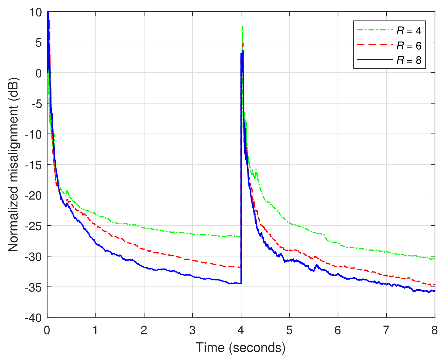
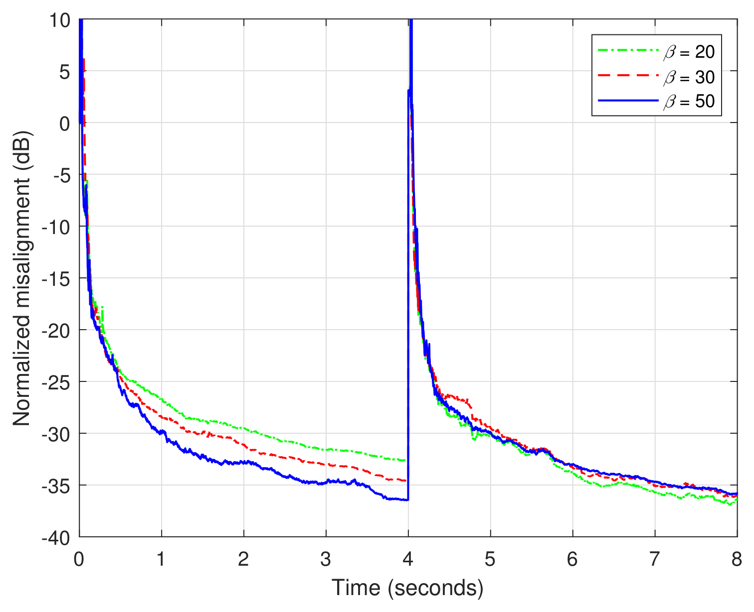
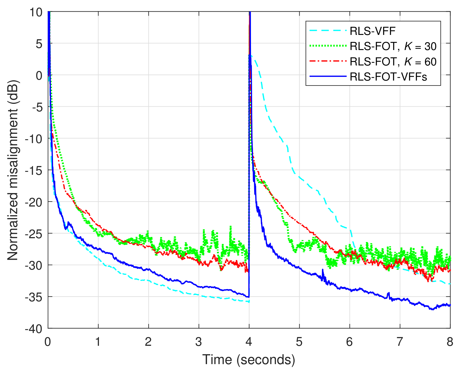
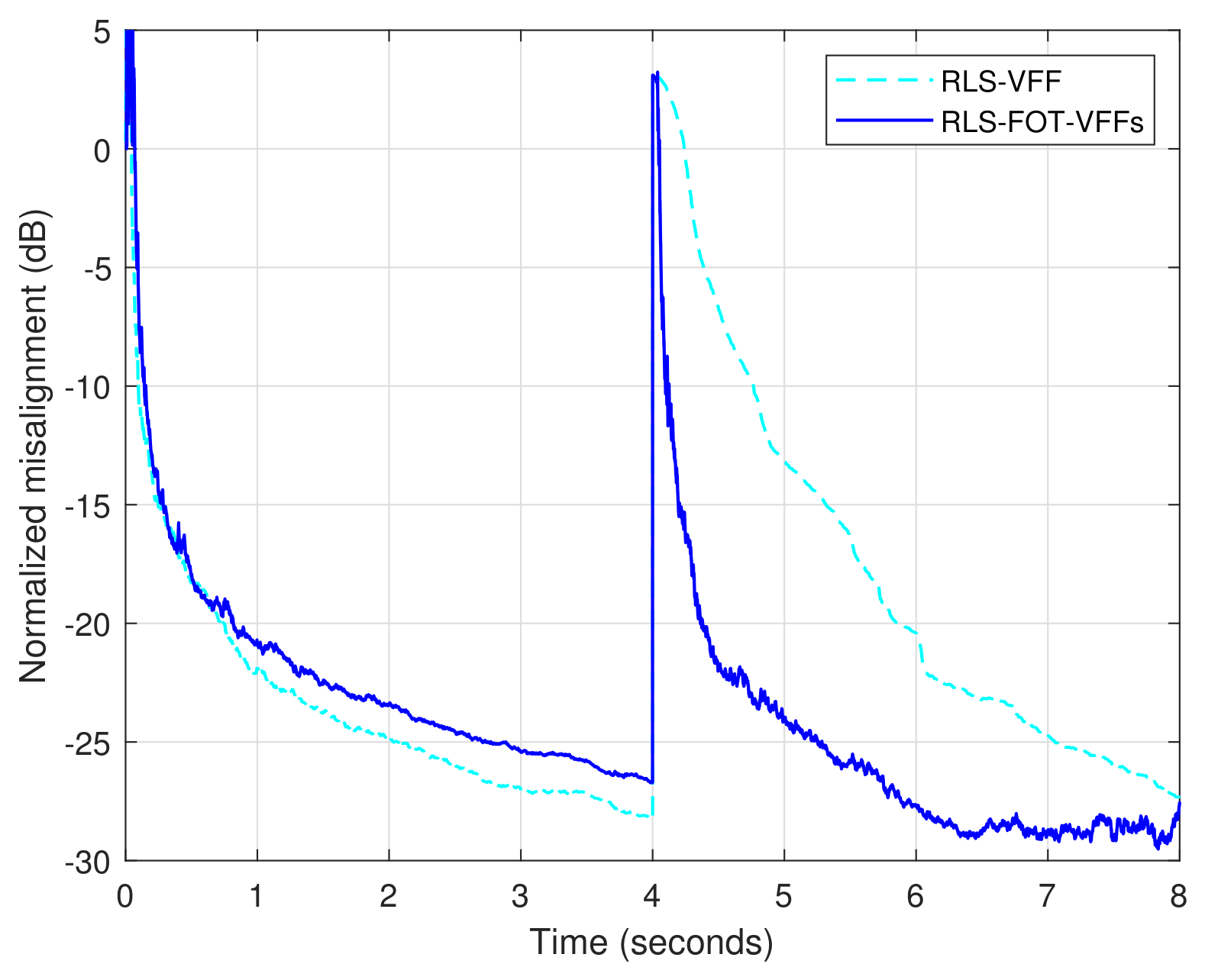
Table 2. The Input Sequences of the RLS-FOT Algorithm.
x ( t ) = x ( t ) x ( t 1 ) x ( t L + 1 ) L = L 11 L 12 L 21 L 22 , R < L 21 L 22 , P < L 12 , Q < L 22 r = 1 , 2 , , R , p = 1 , 2 , , P , q = 1 , 2 , , Q H 22 r p q ( t 1 ) = I L 22 h 21 r q ( t 1 ) h 12 r p ( t 1 ) h 11 r p ( t 1 ) H 21 r p q ( t 1 ) = h 22 r q ( t 1 ) I L 21 h 12 r p ( t 1 ) h 11 r p ( t 1 ) H 12 r p q ( t 1 ) = h 22 r q ( t 1 ) h 21 r q ( t 1 ) I L 12 h 11 r p ( t 1 ) H 11 r p q ( t 1 ) = h 22 r q ( t 1 ) h 21 r q ( t 1 ) h 12 r p ( t 1 ) I L 11 H : p q ( t 1 ) = H 1 p q ( t 1 ) H 2 p q ( t 1 ) H R p q ( t 1 ) , 22 , 21 , 12 , 11 H ̲ 22 ( t 1 ) = p = 1 P H 22 : p 1 ( t 1 ) p = 1 P H 22 : p 2 ( t 1 ) p = 1 P H 22 : p Q ( t 1 ) H ̲ 21 ( t 1 ) = p = 1 P H 21 : p 1 ( t 1 ) p = 1 P H 21 : p 2 ( t 1 ) p = 1 P H 21 : p Q ( t 1 ) H ̲ 12 ( t 1 ) = q = 1 Q H 12 : 1 q ( t 1 ) q = 1 Q H 12 : 2 q ( t 1 ) q = 1 Q H 12 : P q ( t 1 ) H ̲ 11 ( t 1 ) = q = 1 Q H 11 : 1 q ( t 1 ) q = 1 Q H 11 : 2 q ( t 1 ) q = 1 Q H 11 : P q ( t 1 ) x ( t ) = H ̲ ( t 1 ) x ( t ) , 22 , 21 , 12 , 11
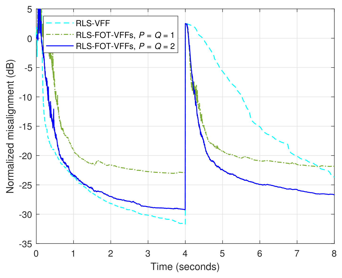
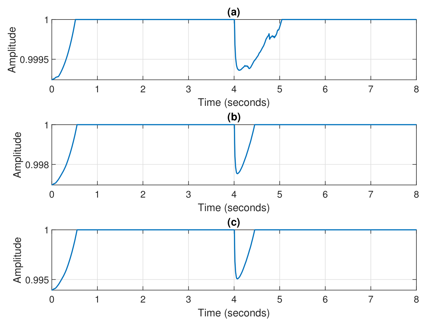
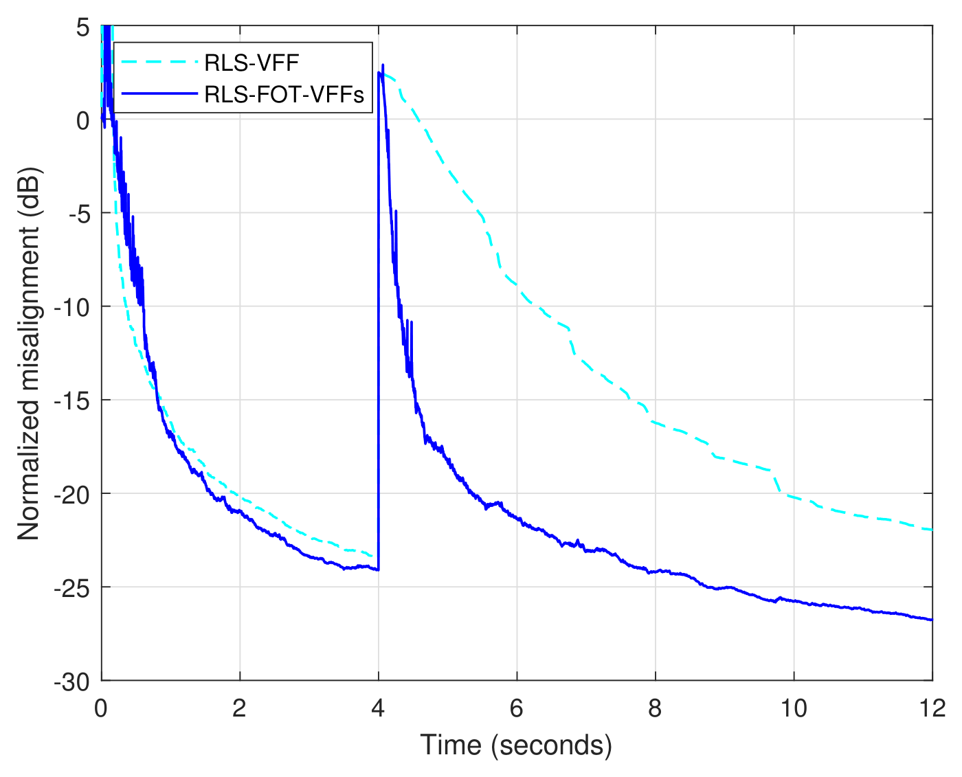
Table 3. RLS-FOT-VFFs Algorithm.
L = L 11 L 12 L 21 L 22 , R < L 21 L 22 , P < L 12 , Q < L 22 Initialization ̲ : R 22 1 ( 0 ) = γ 1 I R Q L 22 , R 21 1 ( 0 ) = γ 1 I R Q L 21 , R 12 1 ( 0 ) = γ 1 I R P L 12 , R 11 1 ( 0 ) = γ 1 I R P L 11 , γ > 0 r = 1 , 2 , , R , p = 1 , 2 , , P , q = 1 , 2 , , Q , 0 < ε 1 h 22 r q ( 0 ) = ε 0 L 22 1 , h 21 r q ( 0 ) = ε 0 L 21 1 , h 12 r p ( 0 ) = ε 0 L 12 1 , h 11 r p ( 0 ) = ε 0 L 11 1 ,
h ̲ ( 0 ) , H ̲ ( 0 ) , with 22 , 21 , 12 , 11  (see Table 1 and Table 2, respectively)
σ e 2 ( 0 ) = σ v 2 ( 0 ) = 0 , 22 , 21 , 12 , 11 , a = 1 1 L , b = 1 1 β L , β 1 ( order of tens ) , 0 < ϵ 1 Iterations ̲ : for t = 1 , 2 , x ( t ) = x ( t ) x ( t 1 ) x ( t L + 1 ) x ( t ) = H ̲ ( t 1 ) x ( t ) e ( t ) = d ( t ) x ( t ) h ̲ ( t 1 ) = e ( t ) σ e 2 ( t ) = a σ e 2 ( t 1 ) + ( 1 a ) e 2 ( t ) σ v 2 ( t ) = b σ v 2 ( t 1 ) + ( 1 b ) e 2 ( t ) α ( t ) = 1 σ v ( t ) ϵ + σ e ( t ) ( bounded   between   0   and   1 ) λ ( t ) : λ 22 ( t ) = 1 α 22 ( t ) R Q L 22 , λ 21 ( t ) = 1 α 21 ( t ) R Q L 21 , λ 12 ( t ) = 1 α 12 ( t ) R P L 12 , λ 11 ( t ) = 1 α 11 ( t ) R P L 11 k ( t ) = R 1 ( t 1 ) x ( t ) λ ( t ) + x ( t ) R 1 ( t 1 ) x ( t ) R 1 ( t ) = 1 λ ( t ) R 1 ( t 1 ) k ( t ) x ( t ) R 1 ( t 1 ) h ̲ ( t ) = h ̲ ( t 1 ) + k ( t ) e ( t )
h 22 r q ( t ) , h 21 r q ( t ) , h 12 r p ( t ) , h 11 r p ( t ) H ̲ ( t )  (see Table 2)
Table 4. Computational Complexities of the Conventional RLS, RLS-FOT [36], RLS-VFF [49], and RLS-FOT-VFFs Algorithms.
AlgorithmsNumber of MultiplicationsNumber of Additions
RLS 2 L 2 + 3 L 2 L 2 + 2 L
RLS-FOT [36] 2 ( R Q L 22 ) 2 + 2 ( R Q L 21 ) 2 + 2 ( R P L 12 ) 2 + 2 ( R P L 11 ) 2 + 2 ( R Q L 22 ) + 2 ( R Q L 21 ) + 2 ( R P L 12 ) + 2 ( R P L 11 ) + min R Q L 22 , R Q L 21 , R P L 12 , R P L 11 + O × 2 ( R Q L 22 ) 2 + 2 ( R Q L 21 ) 2 + 2 ( R P L 12 ) 2 + 2 ( R P L 11 ) 2 + R Q L 22 + R Q L 21 + R P L 12 + R P L 11 + min R Q L 22 , R Q L 21 , R P L 12 , R P L 11 + O +
RLS-VFF [49] 2 L 2 + 3 L + 5 2 L 2 + 2 L + 5
RLS-FOT-VFFs 2 ( R Q L 22 ) 2 + 2 ( R Q L 21 ) 2 + 2 ( R P L 12 ) 2 + 2 ( R P L 11 ) 2 + 2 ( R Q L 22 ) + 2 ( R Q L 21 ) + 2 ( R P L 12 ) + 2 ( R P L 11 ) + min R Q L 22 , R Q L 21 , R P L 12 , R P L 11 + O × + 20 2 ( R Q L 22 ) 2 + 2 ( R Q L 21 ) 2 + 2 ( R P L 12 ) 2 + 2 ( R P L 11 ) 2 + R Q L 22 + R Q L 21 + R P L 12 + R P L 11 + min R Q L 22 , R Q L 21 , R P L 12 , R P L 11 + O + + 20
Disclaimer/Publisher’s Note: The statements, opinions and data contained in all publications are solely those of the individual author(s) and contributor(s) and not of MDPI and/or the editor(s). MDPI and/or the editor(s) disclaim responsibility for any injury to people or property resulting from any ideas, methods, instructions or products referred to in the content.