An Adaptive Multi-Scale Heterogeneous Ensemble Framework for Interpretable Wind Power Forecasting in Sustainable Grids

Abstract
1. Introduction
1.1. Motivation and Challenges
1.2. Literature Review
2. Methodology
2.1. Data Preprocessing
2.2. SHapley Additive exPlanations (SHAP)
2.3. Multivariate Variational Mode Decomposition
- Initialization: Set the number of modes K and the penalty parameter . Initialize all modes (typically in the frequency domain), the shared center frequencies , and the Lagrangian multipliers . Set the iteration index n = 0.
- Mode Update: For each mode k and each channel c, update the mode estimate in the frequency domain using a Wiener-like filter:Here, is the bandwidth penalty parameter, regulating the compactness of the modes.
- Center frequency update: Update the shared center frequency based on the current estimated mode of all channels.This step ensures that each center frequency represents the common spectral center for that oscillatory mode across all variables.
- Lagrange multiplier update: Update the Lagrange multiplier for each channel based on the current reconstruction error to enhance convergence:where serves as the noise tolerance parameter.
- Convergence Check: Iterate steps 2 to 4 until the convergence criterion is satisfied. The criterion is often based on a threshold for the reconstruction error or the magnitude of change in modes between successive iterations:
- Output: Upon convergence, the algorithm outputs the complete set of IMFs for all channels and the final set of center frequencies .
2.4. Intelligent Optimization Algorithm
Multi-Objective Dragonfly Algorithm (MODA)
2.5. Modified Multi-Objective Dragonfly Algorithm (MMODA)
2.5.1. Elite Opposition Learning Strategy
2.5.2. Exponential Function-Based Step-Size Strategy
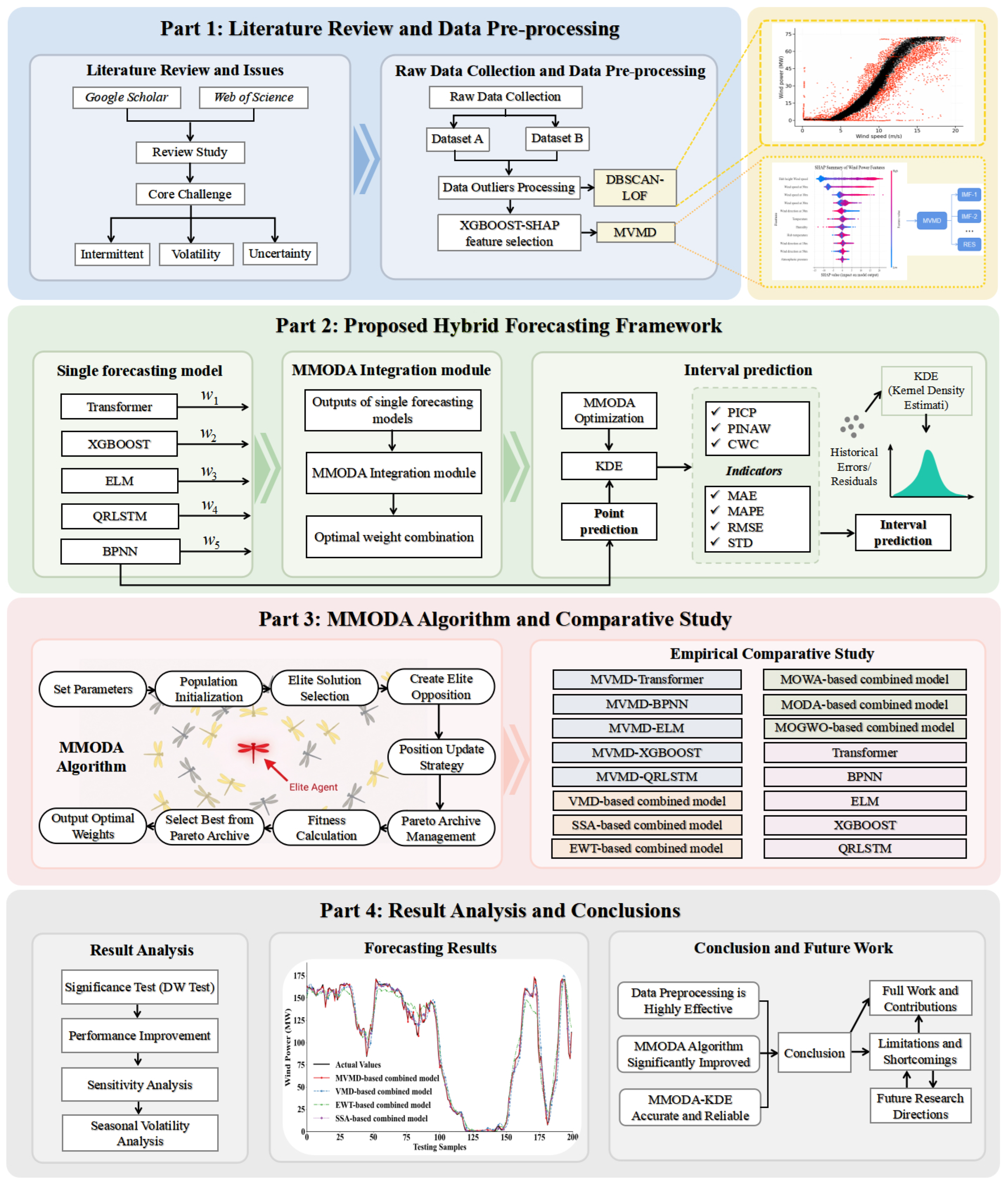
2.6. Methodology and Implementation Flow
- Procedure 1: Data Pretreatment
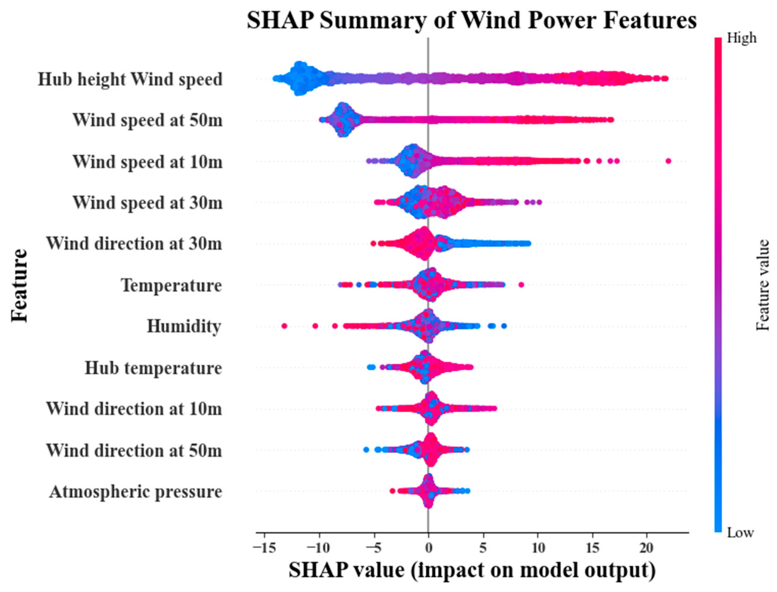
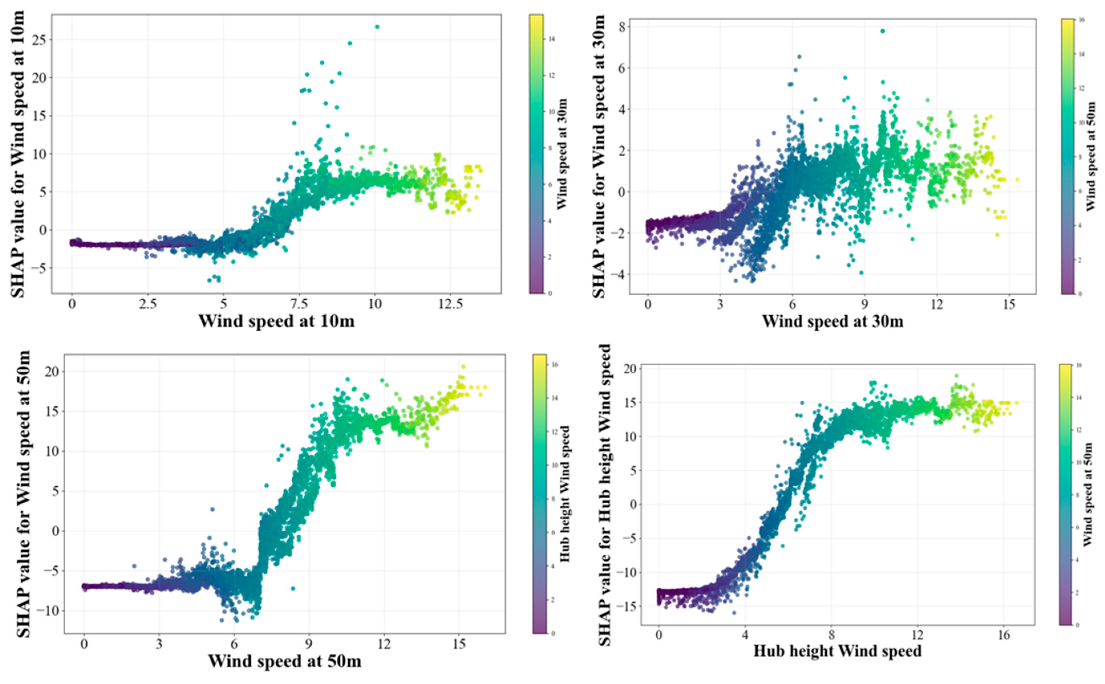
- Procedure 2: Shap-based Feature Selection
- Procedure 3: Theoretical Rationale for Heterogeneous Base Model Selection
- Procedure 4: Model Hyperparameters
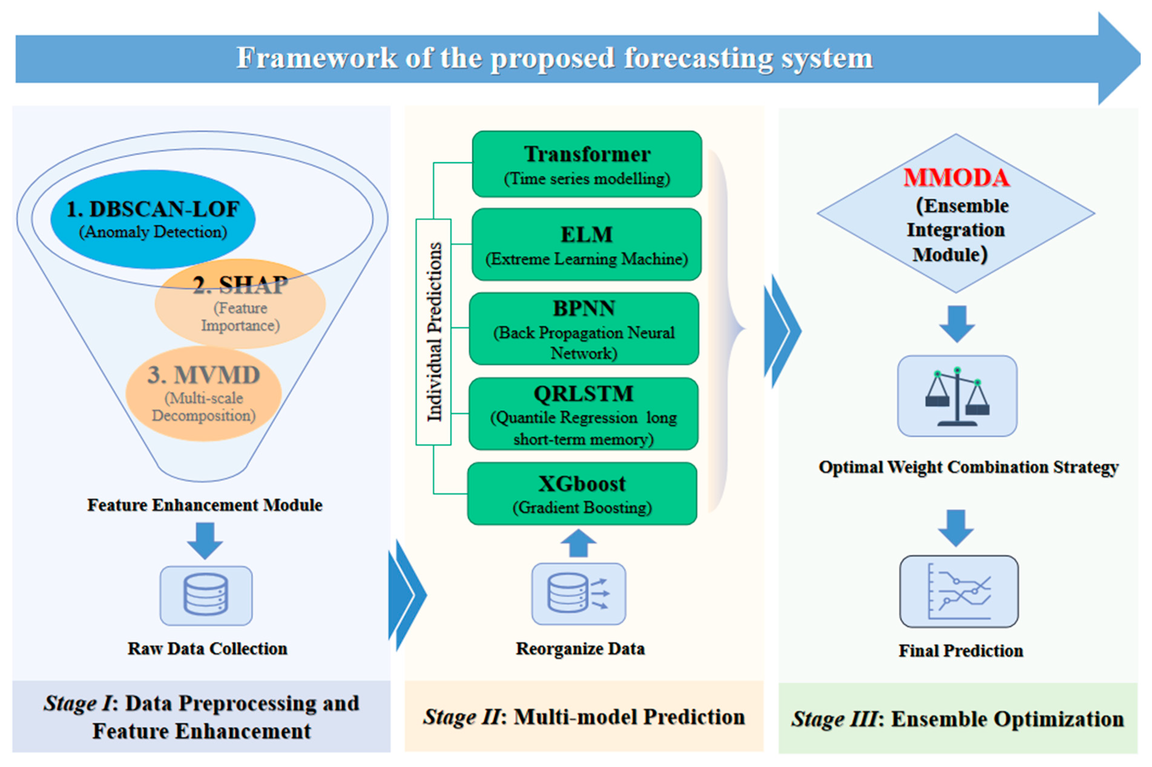
- Procedure 5: Framework of the Proposed Integrated Wind Power Forecasting System
- Procedure 6: Forecasting Performance and Validation of a Combined Model
| Algorithm 1. The Pseudo code of the proposed integrated wind power forecasting system |
| Input: Raw wind farm time-series data, (Decomposition modes), (Penalty factor), (Max iterations), Population size , Elite number , Base models . Output: Optimized weight vector , Multi-step deterministic forecasts, Probabilistic forecasting intervals. //Objective Function Formulation 1: Define Multi-objective function: 2: Accuracy Criterion 3: Stability Criterion //Phase 1: Intelligent Data Refinement 4: Detect global outliers using Adaptive DBSCAN with elbow-point epsilon detection. 5: Filter local anomalies via Local Outlier Factor (LOF) on DBSCAN inliers. 6: Apply Mutual Information (MI) and SHAP to select the most significant meteorological features. //Phase 2: Feature Decomposition & Base Prediction 7: Execute Multivariate VMD (MVMD) to extract robust sub-modes from non-stationary signals. 8: Construct recursive datasets for 1-step, 2-step, and 3-step horizons. 9: Train heterogeneous ensemble (Transformer, BPNN, ELM, XGBoost, and QRLSTM). 10: Generate prediction matrix where each column represents a base model’s output. //Phase 3: MMODA Weight Optimization 11: Initialize dragonfly population and initialize an empty Pareto Archive. 12: While do 13: if then Elite Opposition-Based Learning (EOBL) Strategy 14: Select elite solutions from Archive using Roulette Wheel Selection. 15: Compute dynamic search boundaries based on the current elite set. 16: Generate opposite solutions: . 17: Re-evaluate and update using non-dominated sorting. 18: end if 19: Update social coefficients and inertia weight using adaptive decay. 20: for each individual to SN do 21: if neighbors exist within radius R then 22: Calculate behaviors: Separation (), Alignment (), Cohesion (), Food (), Enemy (). 23: . 24: Update position: . 25: else 26: Perform Lévy flight-based stochastic search. Exploration through Random Walk 27: end if 28: Boundary handling: . 29: end for 30: Update Pareto Archive and prune dense regions using Crowding Distance. 31: . 32: end while //Phase 4: Probabilistic Synthesis & Output 33: Retrieve (Best compromise weights) from the final Pareto Archive. 34: Calculate final deterministic forecast: . 35: Estimate Forecasting Intervals (FIs) using MMODA-optimized Kernel Density Estimation (KDE). 36: , , and interval evaluation metrics (PICP, PINAW). |
3. Experimental Analysis
3.1. Data Source
3.2. Evaluation Criteria for Experimental Validation
3.3. Comparison Forecasting Experiments
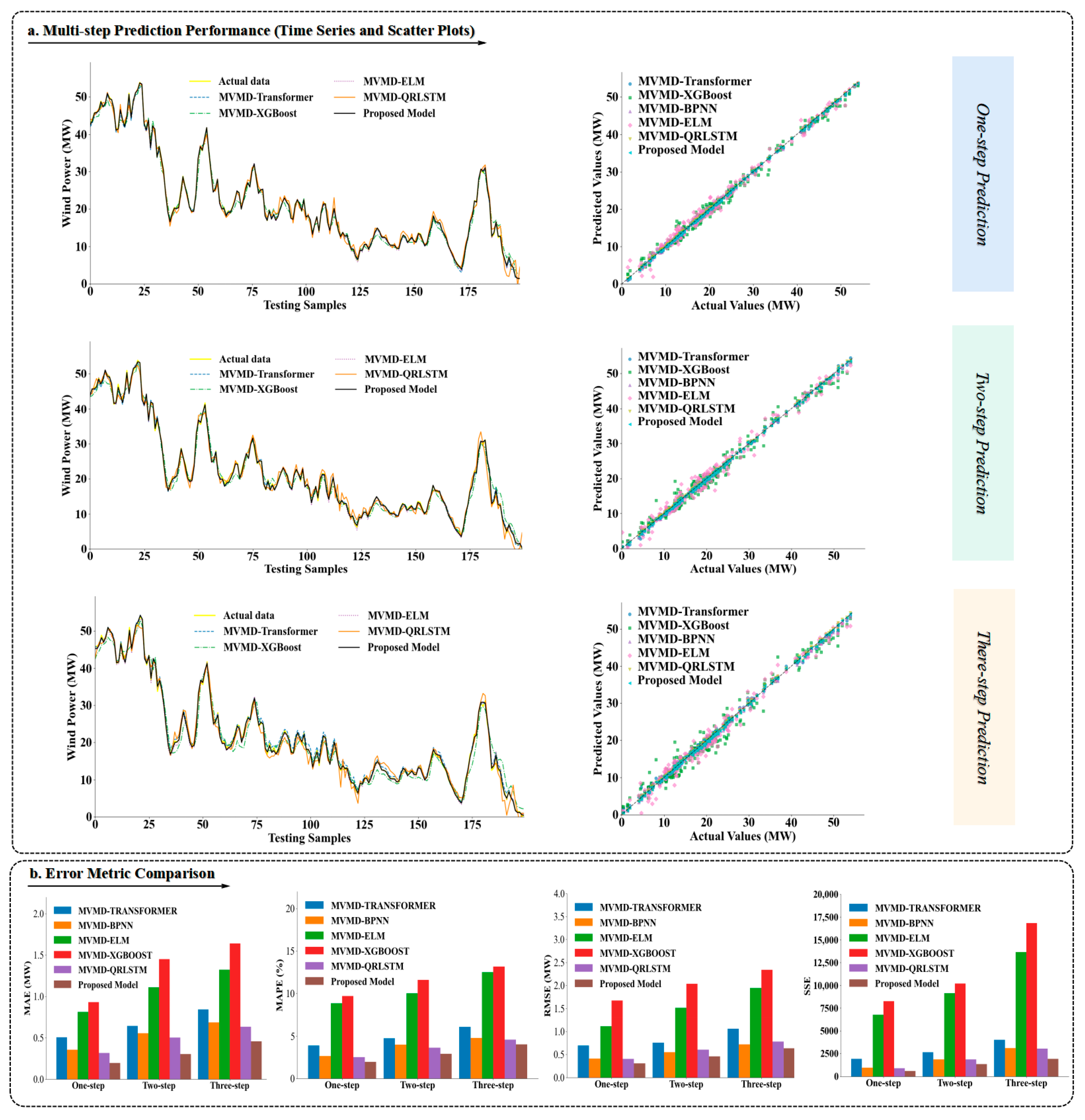
3.3.1. Experiment I: Comparison with Other MVMD-Based Models
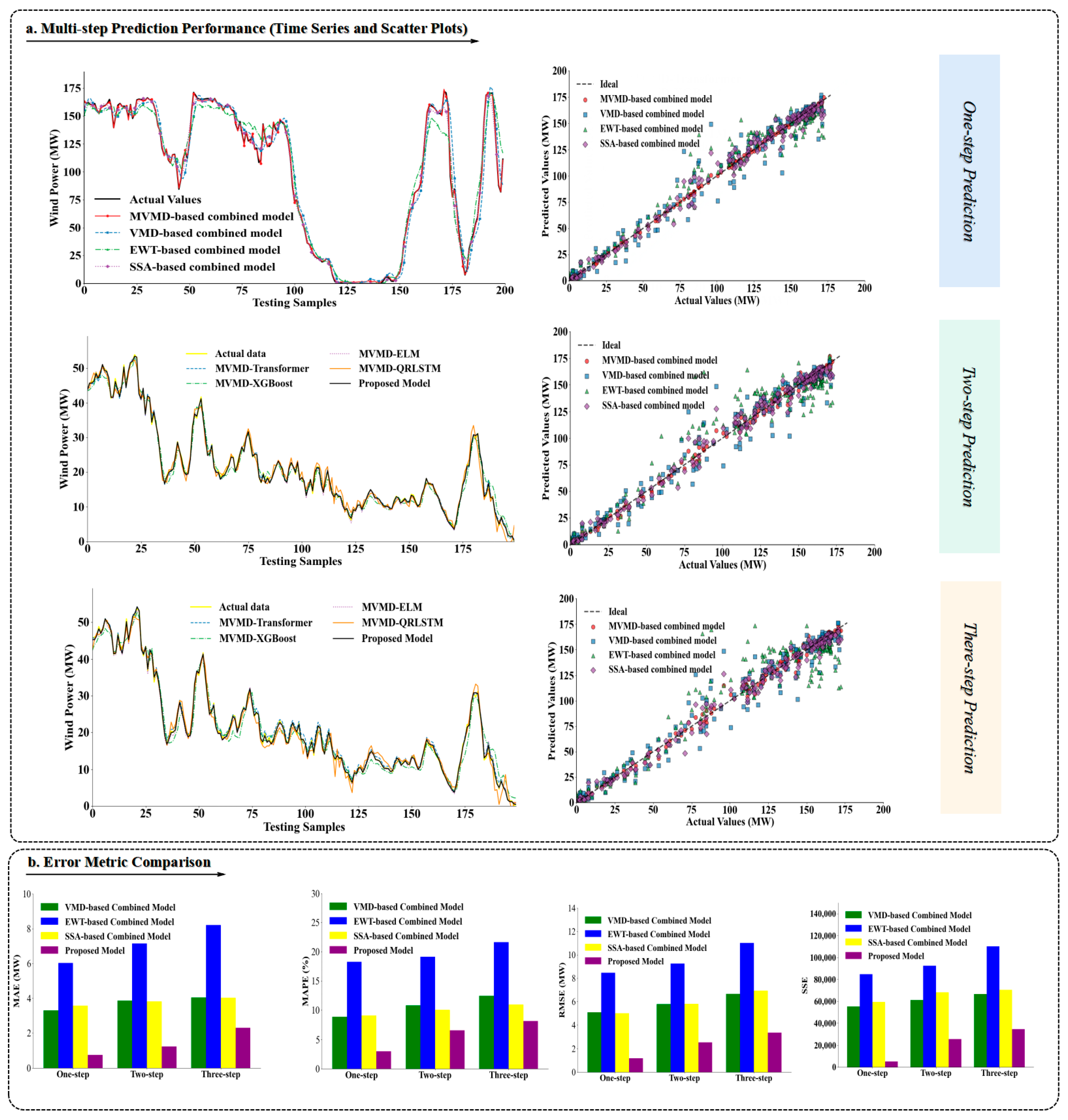
3.3.2. Experiment II: Benchmarking Against Models with Diverse Data Pretreatment
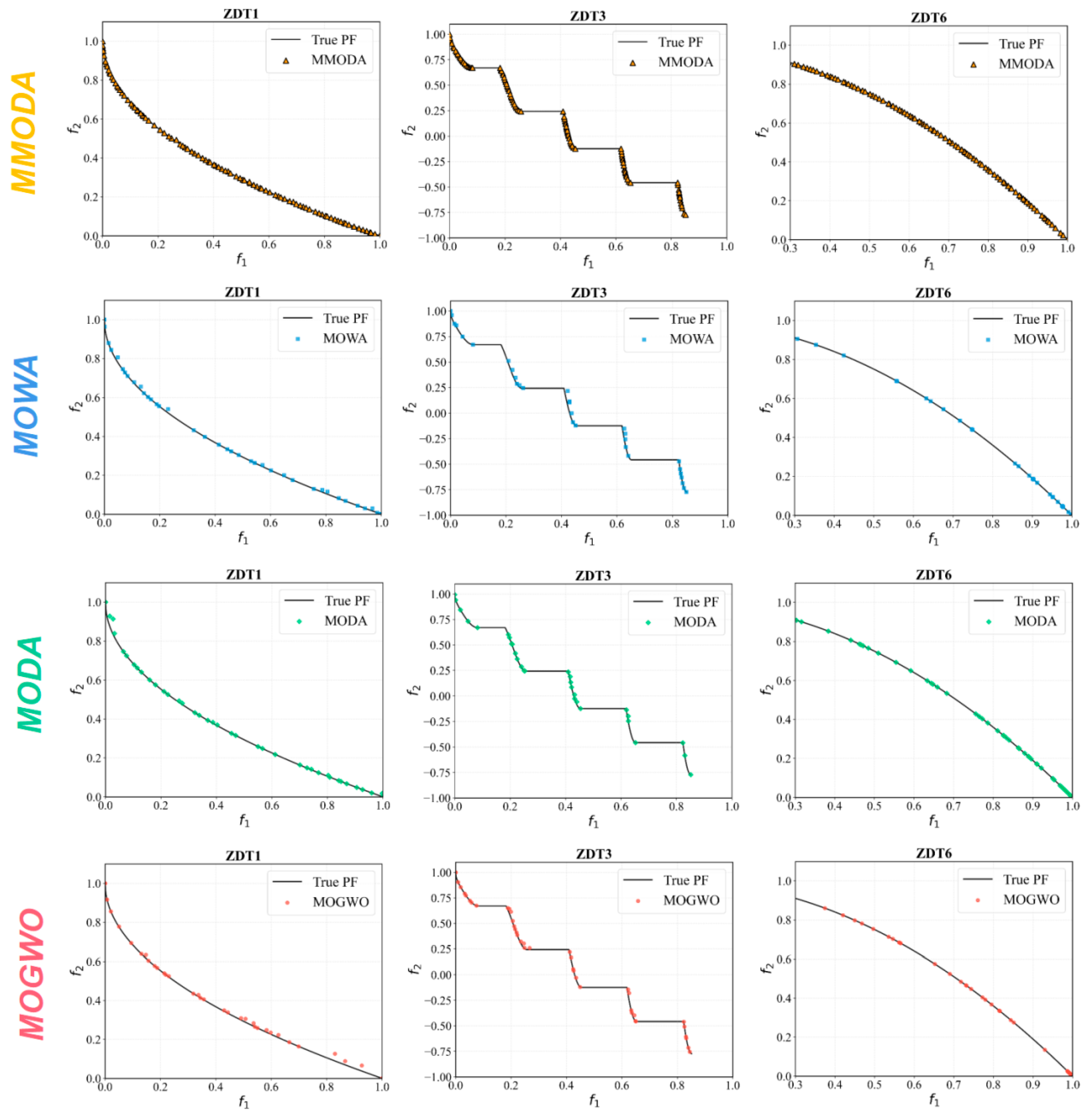
3.3.3. Experiment III: The Advancement of MMODA in Addressing Multi-Objective Optimization Problems
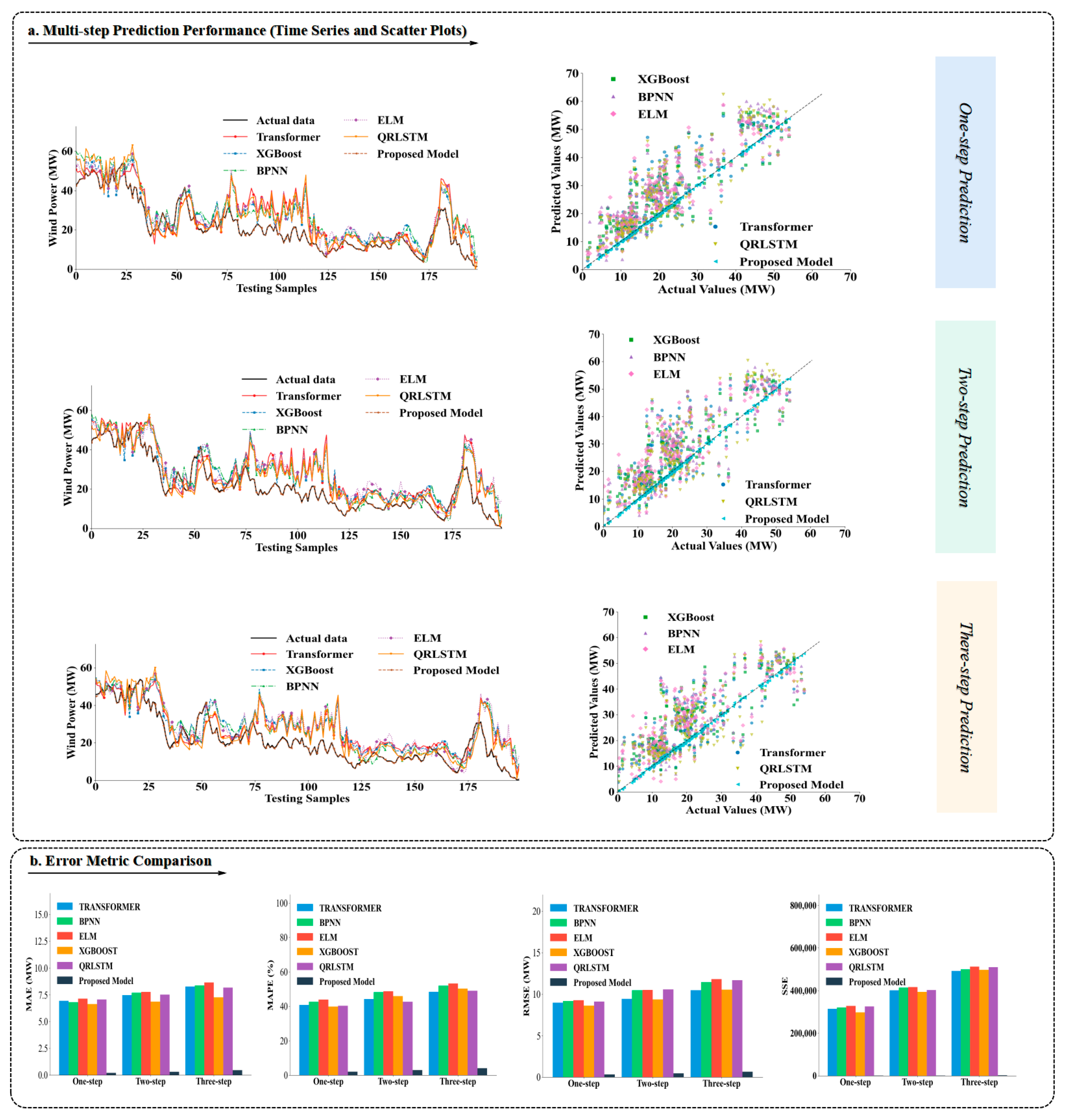
3.3.4. Experiment IV: Benchmarking Against Classic Individual Models
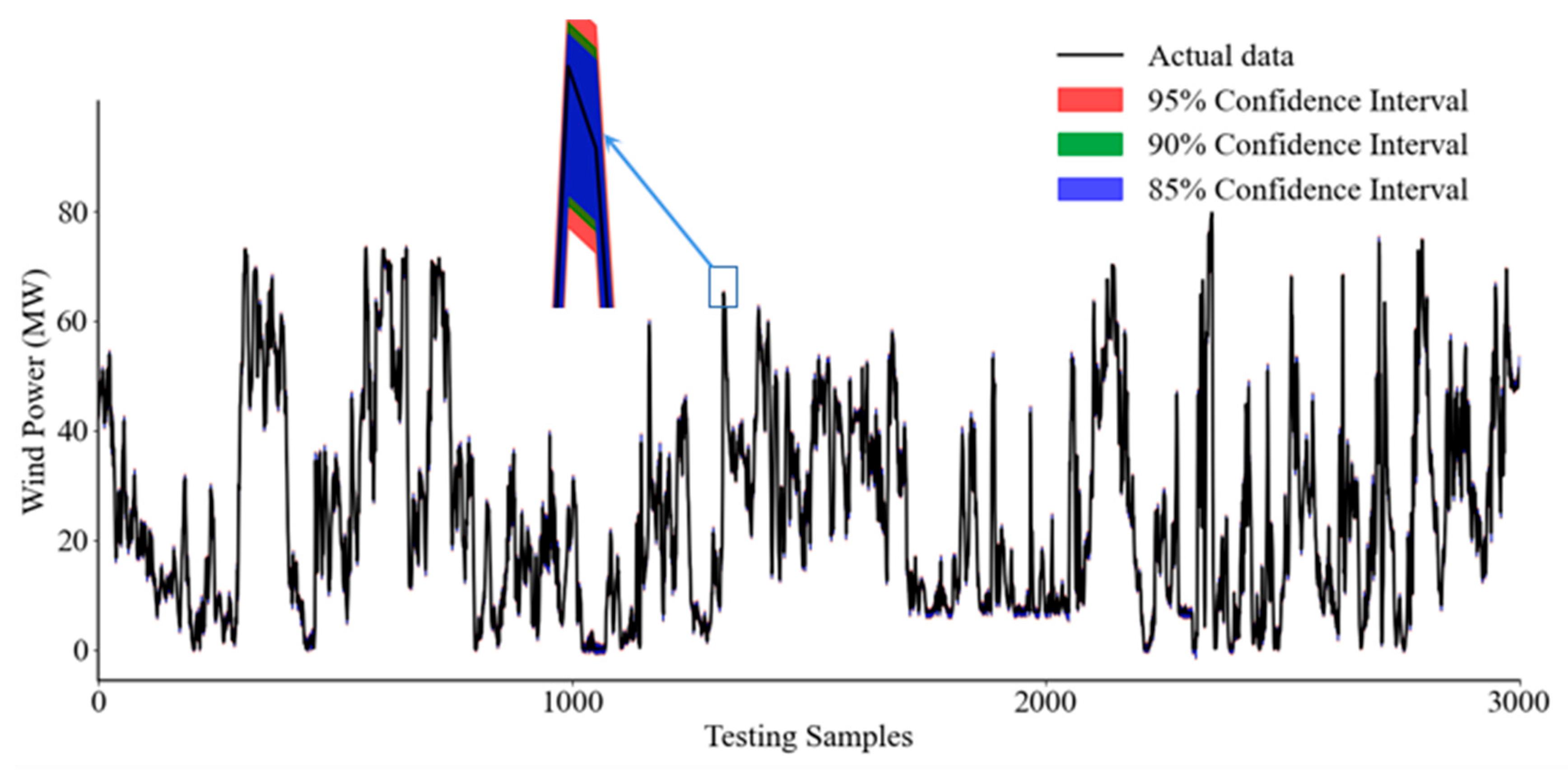
3.4. Interval Forecasting
4. Discussion
4.1. Model Significance Testing: Diebold–Mariano (DM) Test
4.2. Performance Improvements of the Proposed Model
- (a)
- In comparison to the non-optimized hybrid model, the hybrid model MVMD-XGBOOST has the most significant improvement effect. For Site 1, the improvement percentages of PMAE, PMAPE, PRMSE, and PSSE reached 76.7336%, 74.7581%, 77.3163%, and 89.2955% respectively, which shows that the proposed model is obviously superior to the traditional hybrid model in forecast ability.
- (b)
- Compared with the hybrid model integrated by different data preprocessing, the improvement effect is equally significant. For example, in Site 2, the integrated model based on EWT, SSA, and VMD achieved improvement rates of 70.0690%, 62.3612%, and 39.1098% in MAPE, MAE, and RMSE, respectively.
- (c)
- Compared with the hybrid model integrated by different optimization algorithms, the improvement effect is also consistent. Specifically, compared with MODA, the MAE improvement rate of Site 1 reached 31.111%, and the SSE improvement rate of Site 2 was 35.0400%. This indicates that our proposed method has significant advantages. The comparison with MOGWO, MOWA, and other hybrid models also shows a consistent improvement trend.
- (d)
- Compared with the traditional single model, the proposed model has the most significant improvement. In Site 1, the improvement rate of all indicators relative to the Transformer model exceeds 93%. In Station 2, the improvement rate relative to the QRLSTM model also exceeded 89%, indicating that the combined strategy adopted can maximize the forecast accuracy, and is an effective wind speed forecast method.
4.3. Sensitivity Analysis
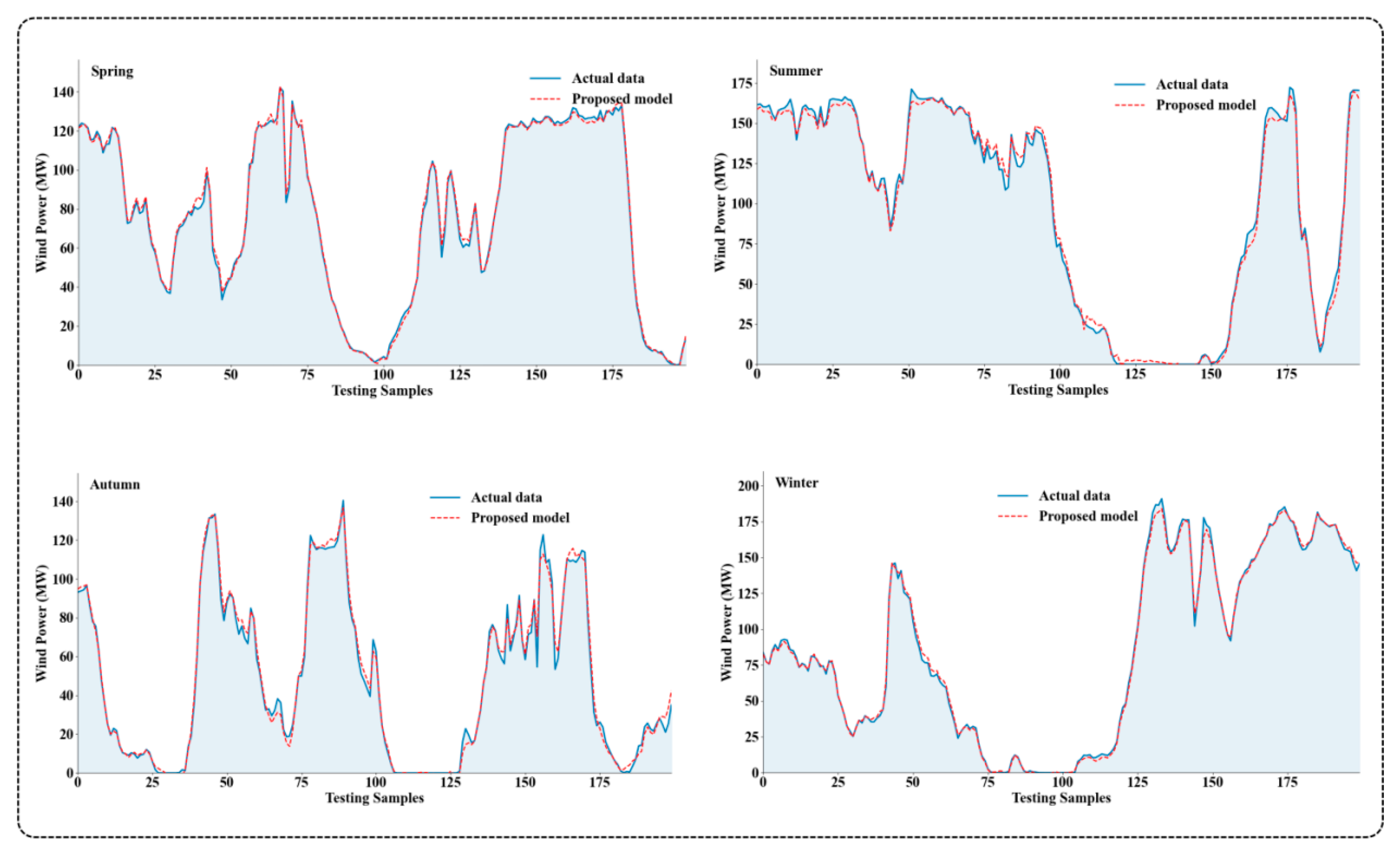
4.4. Seasonal Forecasting Performance Evaluation
4.5. Generalization Ability and Overfitting Analysis
4.6. Run Time
5. Conclusions
Author Contributions
Funding
Data Availability Statement
Conflicts of Interest
References
- Wang, Y.; Guo, C.H.; Chen, X.J.; Jia, L.Q.; Guo, X.N.; Chen, R.S.; Zhang, M.-S.; Chen, Z.-Y.; Wang, H.-D. Carbon peak and carbon neutrality in China: Goals, implementation path and prospects. China Geol. 2021, 4, 720–746. [Google Scholar] [CrossRef] [Scilit]
- Shi, C.; Zhi, J.; Yao, X.; Zhang, H.; Yu, Y.; Zeng, Q.; Li, L.; Zhang, Y. How can China achieve the 2030 carbon peak goal—A crossover analysis based on low-carbon economics and deep learning. Energy 2023, 269, 126776. [Google Scholar] [CrossRef] [Scilit]
- Shi, H.; Heng, J.; Duan, H.; Li, H.; Chen, W.; Wang, P.; Cui, L.; Wang, S. Critical mineral constraints pressure energy transition and trade toward the Paris Agreement climate goals. Nat. Commun. 2025, 16, 4496. [Google Scholar] [CrossRef] [Scilit]
- Global Wind Energy Council. Global Wind Statistics. 2024. Available online: https://www.gwec.net/reports/globalwindreport#Download (accessed on 21 May 2026).
- Wang, Y.; Zou, R.; Liu, F.; Zhang, L.; Liu, Q. A review of wind speed and wind power forecasting with deep neural networks. Appl. Energy 2021, 304, 117766. [Google Scholar] [CrossRef] [Scilit]
- Mayer, M.J.; Yang, D. Pairing ensemble numerical weather prediction with ensemble physical model chain for probabilistic photovoltaic power forecasting. Renew. Sustain. Energy Rev. 2023, 175, 113171. [Google Scholar] [CrossRef] [Scilit]
- Tang, Y.; Guo, Y.; Shen, G.; Zhang, Z. Wind Power Forecasting: A Multi-task Learning Framework Based on Hybrid Model and Knowledge Sharing. Appl. Soft Comput. 2025, 189, 114532. [Google Scholar] [CrossRef] [Scilit]
- He, B.; Ye, L.; Pei, M.; Lu, P.; Dai, B.; Li, Z.; Wang, K. A combined model for short-term wind power forecasting based on the analysis of numerical weather prediction data. Energy Rep. 2022, 8, 929–939. [Google Scholar] [CrossRef] [Scilit]
- Choi, S.; Jung, E.S. Optimizing numerical weather prediction model performance using machine learning techniques. IEEE Access 2023, 11, 86038–86055. [Google Scholar] [CrossRef] [Scilit]
- Yang, M.; Guo, Y.; Huang, Y. Wind power ultra-short-term prediction method based on NWP wind speed correction and double clustering division of transitional weather process. Energy 2023, 282, 128947. [Google Scholar] [CrossRef] [Scilit]
- Tyass, I.; Khalili, T.; Rafik, M.; Abdelouahed, B.; Raihani, A.; Mansouri, K. Wind Speed Prediction Based on Statistical and Deep Learning Models. Int. J. Renew. Energy Dev. 2023, 12, 288–299. [Google Scholar] [CrossRef] [Scilit]
- Yan, S.; Hu, M. A multi-stage planning method for distribution networks based on ARIMA with error gradient sampling for source–load prediction. Sensors 2022, 22, 8403. [Google Scholar] [CrossRef] [Scilit]
- Mandal, A.K.; Sen, R.; Goswami, S.; Chakraborty, B. Comparative study of univariate and multivariate long short-term memory for very short-term forecasting of global horizontal irradiance. Symmetry 2021, 13, 1544. [Google Scholar] [CrossRef] [Scilit]
- Huang, Y.; Dai, X.; Wang, Q.; Zhou, D. A hybrid model for carbon price forecasting using GARCH and long short-term memory network. Appl. Energy 2021, 285, 116485. [Google Scholar] [CrossRef] [Scilit]
- Pleños, M. Time series forecasting using holt-winters exponential smoothing: Application to abaca fiber data. Zesz. Nauk. SGGW W Warszawie-Probl. Rol. Swiat. 2022, 22, 17–29. [Google Scholar] [CrossRef] [Scilit]
- Zhang, W.; Lin, Z.; Liu, X. Short-term offshore wind power forecasting-A hybrid model based on Discrete Wavelet Transform (DWT), Seasonal Autoregressive Integrated Moving Average (SARIMA), and deep-learning-based Long Short-Term Memory (LSTM). Renew. Energy 2022, 185, 611–628. [Google Scholar] [CrossRef] [Scilit]
- Tyass, I.; Bellat, A.; Raihani, A.; Mansouri, K.; Khalili, T. Wind speed prediction based on seasonal ARIMA model. In E3S Web of Conferences; EDP Sciences: London, UK, 2022; Volume 336, p. 00034. [Google Scholar]
- Al-Gounmeein, R.S.; Ismail, M.T.; Al-Hasanat, B.N.; Awajan, A.M. Improving models accuracy using kalman filter and holt-winters approaches based on ARFIMA Models. IAENG Int. J. Appl. Math. 2023, 53, 98–107. [Google Scholar]
- Zhang, S.; Liu, M.; Xie, M.; Lin, S. Two-stage short-term wind power probabilistic prediction using natural gradient boosting combined with neural network. Appl. Soft Comput. 2024, 159, 111669. [Google Scholar] [CrossRef] [Scilit]
- Ay, A.; Önal, K.; Top, A.; Haydaroğlu, C.; Kılıç, H.; Yıldırım, Ö. Comparative Deep Learning Models for Short-Term Wind Power Forecasting: A Real-World Case Study from Tokat Wind Farm, Türkiye. Symmetry 2025, 18, 11. [Google Scholar] [CrossRef] [Scilit]
- Hou, X.; Li, Y.; Liu, Z. An Enhanced Polar Lights Optimization Algorithm with Symmetry Mechanisms for Global Optimization and Its Application to Wind Power Forecasting. Symmetry 2025, 18, 61. [Google Scholar] [CrossRef] [Scilit]
- Khazaei, S.; Ehsan, M.; Soleymani, S.; Mohammadnezhad-Shourkaei, H. A high-accuracy hybrid method for short-term wind power forecasting. Energy 2022, 238, 122020. [Google Scholar] [CrossRef] [Scilit]
- Qu, K.; Si, G.; Shan, Z.; Kong, X.; Yang, X. Short-term forecasting for multiple wind farms based on transformer model. Energy Rep. 2022, 8, 483–490. [Google Scholar] [CrossRef] [Scilit]
- Zheng, X.; Guan, S.; Zhou, Y. Attention-enhanced kolmogorov–arnold networks for accurate wind power prediction. Appl. Soft Comput. 2026, 190, 114637. [Google Scholar] [CrossRef] [Scilit]
- Suo, L.; Peng, T.; Song, S.; Zhang, C.; Wang, Y.; Fu, Y.; Nazir, M.S. Wind speed prediction by a swarm intelligence based deep learning model via signal decomposition and parameter optimization using improved chimp optimization algorithm. Energy 2023, 276, 127526. [Google Scholar] [CrossRef] [Scilit]
- Hu, J.; Deng, Y.; Che, J. A novel wind power interval prediction method based on neural ensemble search and dynamic conformalized quantile regression. Appl. Soft Comput. 2025, 180, 113476. [Google Scholar] [CrossRef] [Scilit]
- Zhou, D.; Jia, Y.; Liu, G.; Li, J.; Xi, K.; Wang, Z.; Wang, X. Research on an Ultra-Short-Term Wind Power Forecasting Model Based on Multi-Scale Decomposition and Fusion Framework. Symmetry 2026, 18, 253. [Google Scholar] [CrossRef] [Scilit]
- Hanifi, S.; Cammarono, A.; Zare-Behtash, H. Advanced hyperparameter optimization of deep learning models for wind power prediction. Renew. Energy 2024, 221, 119700. [Google Scholar] [CrossRef] [Scilit]
- Guo, H.; Wang, J.; Li, Z.; Jin, Y. A multivariable hybrid prediction system of wind power based on outlier test and innovative multi-objective optimization. Energy 2022, 239, 122333. [Google Scholar] [CrossRef] [Scilit]
- Wang, J.; Wu, X.; Chen, M. Dynamic ensemble point-interval wind speed prediction system for data drift: Adaptive real-time feature decoupling and multi-level information fusion quantile regression. Appl. Soft Comput. 2026, 190, 114615. [Google Scholar] [CrossRef] [Scilit]
- Kumar, B.; Yadav, N. A novel hybrid algorithm based on Empirical Fourier decomposition and deep learning for wind speed forecasting. Energy Convers. Manag. 2024, 300, 117891. [Google Scholar] [CrossRef] [Scilit]
- Xiong, Z.; Yao, J.; Huang, Y.; Yu, Z.; Liu, Y. A wind speed forecasting method based on EMD-MGM with switching QR loss function and novel subsequence superposition. Appl. Energy 2024, 353, 122248. [Google Scholar] [CrossRef] [Scilit]
- He, Y.; Wang, Y. Short-term wind power prediction based on EEMD–LASSO–QRNN model. Appl. Soft Comput. 2021, 105, 107288. [Google Scholar] [CrossRef] [Scilit]
- Lei, P.; Ma, F.; Zhu, C.; Li, T. LSTM short-term wind power prediction method based on data preprocessing and variational modal decomposition for soft sensors. Sensors 2024, 24, 2521. [Google Scholar] [CrossRef] [Scilit]
- Xie, B.; Shi, S.; Liu, W. Integrated forecasting of marine renewable power: An adaptively Bayesian-optimized MVMD-LSTM framework for wind-solar-wave energy. Sustain. Energy Technol. Assess. 2025, 84, 104753. [Google Scholar] [CrossRef] [Scilit]
- Xian, H.; Che, J. Unified whale optimization algorithm based multi-kernel SVR ensemble learning for wind speed forecasting. Appl. Soft Comput. 2022, 130, 109690. [Google Scholar] [CrossRef] [Scilit]
- Mirjalili, S. Dragonfly algorithm: A new meta-heuristic optimization technique for solving single-objective, discrete, and multi-objective problems. Neural Comput. Appl. 2016, 27, 1053–1073. [Google Scholar] [CrossRef] [Scilit]
- Wu, H.; Gao, X.Z.; Li, K.; Heng, J.N. An improved brain-motivated network for forecasting day-ahead stock prices of electricity companies. Knowl.-Based Syst. 2025, 325, 114040. [Google Scholar] [CrossRef] [Scilit]
- Shambour, Q.; Al-Zyoud, M.; Almomani, O. Quantum-inspired hybrid metaheuristic feature selection with SHAP for optimized and explainable spam detection. Symmetry 2025, 17, 1716. [Google Scholar] [CrossRef] [Scilit]
- Jiang, T.; Liu, B.; Li, X.; Mazza, A.; Li, G.; Pons, E.; Huang, T. Subsynchronous oscillation source location in power system with high penetration of wind power using multivariate variational mode decomposition. IEEE Trans. Power Syst. 2025, 40, 4971–4983. [Google Scholar] [CrossRef] [Scilit]
- Bates, J.M.; Granger, C.W. The combination of forecasts. J. Oper. Res. Soc. 1969, 20, 451–468. [Google Scholar] [CrossRef] [Scilit]
- Nascimento, E.G.S.; de Melo, T.A.; Moreira, D.M. A transformer-based deep neural network with wavelet transform for forecasting wind speed and wind energy. Energy 2023, 278, 127678. [Google Scholar] [CrossRef] [Scilit]
- Shang, Y.; Miao, L.; Shan, Y.; Gnyawali, K.R.; Zhang, J.; Kattel, G. A hybrid ultra-short-term and short-term wind speed forecasting method based on CEEMDAN and GA-BPNN. Weather Forecast. 2022, 37, 415–428. [Google Scholar] [CrossRef] [Scilit]
- Wang, J.; Niu, X.; Zhang, L.; Liu, Z.; Huang, X. A wind speed forecasting system for the construction of a smart grid with two-stage data processing based on improved ELM and deep learning strategies. Expert Syst. Appl. 2024, 241, 122487. [Google Scholar] [CrossRef] [Scilit]
- Wu, X.; Cheng, H.; Wu, B.; Jiang, N.; Huang, Y. A regional XGBoost-based predictive model for the cumulative hours of wind speed levels. Atmos. Res. 2026, 327, 108336. [Google Scholar] [CrossRef] [Scilit]
- Zhu, J.; He, Y. A Large-Scale Multiobjective Evolutionary Quantile Estimation Model for Wind Power Probabilistic Forecasting. IEEE Trans. Evol. Comput. 2024, 29, 2244–2257. [Google Scholar] [CrossRef] [Scilit]
- Liu, Z.; Jiang, P.; Zhang, L.; Niu, X. A combined forecasting model for time series: Application to short-term wind speed forecasting. Appl. Energy 2020, 259, 114137.1–114137.25. [Google Scholar] [CrossRef] [Scilit]



| Method Category | Feature | Advantage | Shortcoming |
|---|---|---|---|
| Physics-based methods (such as NWP) | Based on meteorological principles and fluid dynamics | (1) Good long-term forecast effect (2) Clear physical meaning | (1) The calculation is complex and time-consuming (2) High demand for data (3) Short-term forecast |
| Time series method (such as ARIMA, GARCH) | Linear model, parameter estimation | (1) High efficiency of short-term forecast (2) Mature mathematical theory (3) Only historical power data is needed | (1) Difficult to capture complex nonlinear relationships (2) Poor precision of long-term forecast (3) Weak handling of multiple variables |
| Intelligent algorithm (such as machine learning, deep learning) | Deep structure, automatic feature extraction | (1) Powerful nonlinear fitting ability (2) Excellent fault tolerance and generalization (3) Time-dependent capture accuracy | (1) Requires access to extensive, high-quality data (2) High risk of overfitting (3) Poor black box and interpretability |
| mixed methods | Multi-technology integration, complementing each other’s strengths and weaknesses | (1) Complementary advantages, balancing (2) Bias and variance Strong flexibility (3) Better robustness | (1) High system complexity (2) The computational cost may be higher (3) Subjective weight allocation |
| Parameter | Transformer | XGBoost | BPNN | ELM | QRLSTM |
|---|---|---|---|---|---|
| Network Architecture | 2 Attention blocks + Flatten + 2 Dense (256, 128) | Gradient boosting trees (1500 trees, max depth 7) | 3 Dense layers (256, 128) | Single hidden-layer feedforward (500 hidden neurons) | Bidirectional LSTM (192 units) + Attention + Dense (128, 64) |
| Activation Function | ReLU | - | tanh | ReLU | Swish |
| Dropout Rate | 0.3 | - | - | - | 0.2 |
| Optimizer | Adam | - | Adam | Adam | Adam |
| Learning Rate | 0.0005 | 0.015 (tree learning rate) | 0.001 | - | 0.0005 |
| Batch Size | 128 | - | 200 | - | 128 |
| Loss Function | MAE | MAE | MAE | MAE | MAE |
| Output Layer | Dense | Weighted sum of tree leaves | Dense | Linear weighted sum | Dense |
| Metric | Definition | Equation |
|---|---|---|
| MAE | Average value of absolute error between forecast value and true value | |
| MAPE | Average percentage of relative error between forecast value and true value | |
| RMSE | The square root of the mean value of the square sum of the errors between the forecast value and the true value | |
| SSE | Sum of squares of errors between forecast value and true value |
| Model | Decomposition Model | Prediction Model | Optimization Model |
|---|---|---|---|
| #1 | MVMD | Transformer, BPNN, ELM, XGBoost, QRLSTM | MMODA |
| #2 | MVMD | Transformer | |
| #3 | BPNN | ||
| #4 | ELM | ||
| #5 | XGBoost | ||
| #6 | QRLSTM | ||
| #7 | VMD | Transformer, BPNN, ELM, XGBoost, QRLSTM | MMODA |
| #8 | EWT | Transformer, BPNN, ELM, XGBoost, QRLSTM | |
| #9 | SSA | Transformer, BPNN, ELM, XGBoost, QRLSTM | |
| #10 | MVMD | Transformer, BPNN, ELM, XGBoost, QRLSTM | MOGWO |
| #11 | Transformer, BPNN, ELM, XGBoost, QRLSTM | MOWA | |
| #12 | Transformer, BPNN, ELM, XGBoost, QRLSTM | MODA | |
| #13 | Transformer | ||
| #14 | BPNN | ||
| #15 | ELM | ||
| #16 | XGBoost | ||
| #17 | QRLSTM |
| Algorithm | Parameters | Value |
|---|---|---|
| MMODA | Iteration Number | 200 |
| Archive Size | 100 | |
| Dragonfly Number | 200 | |
| MVMD | Number of Modes (K) | 6 |
| Penalty Factor (α) | 200 | |
| Convergence Tolerance (τ) | 1 × 10⁻⁷ | |
| Iteration Number | 800 |
| Dataset | Model | 1-Step | 2-Step | 3-Step | |||||||||
|---|---|---|---|---|---|---|---|---|---|---|---|---|---|
| MAE | MAPE | RMSE | SSE | MAE | MAPE | RMSE | SSE | MAE | MAPE | RMSE | SSE | ||
| Site 1 | #2 | 0.51 | 3.87 | 0.70 | 1938.86 | 0.64 | 4.74 | 0.76 | 2651.08 | 0.84 | 6.07 | 1.06 | 4034.98 |
| #3 | 0.36 | 2.64 | 0.41 | 949.71 | 0.56 | 3.97 | 0.55 | 1869.65 | 0.69 | 4.78 | 0.72 | 3106.50 | |
| #4 | 0.81 | 8.85 | 1.12 | 6768.19 | 1.11 | 10.03 | 1.51 | 9129.16 | 1.33 | 12.52 | 1.95 | 13,659.40 | |
| #5 | 0.93 | 9.71 | 1.68 | 8272.10 | 1.45 | 11.60 | 2.04 | 10,202.56 | 1.64 | 13.18 | 2.34 | 16,831.88 | |
| #6 | 0.32 | 2.51 | 0.41 | 893.30 | 0.50 | 3.63 | 0.60 | 1859.47 | 0.63 | 4.57 | 0.78 | 3058.16 | |
| #1 | 0.20 | 1.96 | 0.31 | 612.05 | 0.31 | 2.90 | 0.46 | 1349.40 | 0.46 | 4.02 | 0.63 | 1939.05 | |
| Site 2 | #2 | 1.79 | 5.94 | 2.25 | 12,211.10 | 2.15 | 6.22 | 2.78 | 19,690.33 | 2.68 | 7.17 | 3.37 | 27,806.99 |
| #3 | 1.45 | 4.07 | 1.86 | 9696.00 | 1.93 | 5.86 | 2.55 | 17,294.83 | 2.27 | 6.61 | 3.02 | 25,610.00 | |
| #4 | 2.44 | 7.80 | 3.11 | 20,123.00 | 2.82 | 9.28 | 4.35 | 32,993.84 | 3.29 | 10.86 | 5.48 | 54,264.30 | |
| #5 | 3.92 | 10.41 | 4.78 | 58,981.02 | 4.37 | 12.30 | 6.50 | 72,845.71 | 6.44 | 13.06 | 8.05 | 102,647.72 | |
| #6 | 1.39 | 3.92 | 1.98 | 9846.33 | 1.90 | 5.33 | 2.71 | 17,541.32 | 2.33 | 6.45 | 3.16 | 25,513.92 | |
| #1 | 1.03 | 3.06 | 1.45 | 7677.29 | 1.62 | 4.61 | 2.33 | 15,598.02 | 2.00 | 5.59 | 2.65 | 22,066.52 | |
| Algorithm | Parameters | Value |
|---|---|---|
| MMODA | Iteration Number | 200 |
| Archive Size | 100 | |
| Dragonfly Number | 200 | |
| MVMD | Number of Modes (K) | 6 |
| Penalty Factor (α) | 200 | |
| Convergence Tolerance (τ) | 1 × 10⁻⁷ | |
| Iteration Number | 800 | |
| VMD | Number of Modes (K) | 6 |
| Penalty Factor (α) | 2000 | |
| Convergence Tolerance (τ) | 1 × 10⁻⁷ | |
| EWT | Number of decomposed modes | 6 |
| SSA | Window Length | 24 |
| Principal Component Decomposition Number | 6 |
| Dataset | Model | 1-Step | 2-Step | 3-Step | |||||||||
|---|---|---|---|---|---|---|---|---|---|---|---|---|---|
| MAE | MAPE | RMSE | SSE | MAE | MAPE | RMSE | SSE | MAE | MAPE | RMSE | SSE | ||
| Site 1 | #7 | 1.87 | 11.55 | 2.79 | 28,527.41 | 2.03 | 12.35 | 3.03 | 31,768.26 | 2.10 | 13.17 | 3.06 | 34,091.31 |
| #8 | 4.00 | 24.19 | 5.81 | 98,205.49 | 4.49 | 28.46 | 6.49 | 126,804.46 | 5.00 | 31.54 | 7.20 | 158,426.32 | |
| #9 | 2.34 | 13.13 | 3.61 | 46,432.62 | 2.42 | 13.56 | 3.74 | 50,770.42 | 2.41 | 13.62 | 4.00 | 52,759.14 | |
| #1 | 0.20 | 1.96 | 0.31 | 612.05 | 0.31 | 2.90 | 0.46 | 1349.40 | 0.46 | 4.02 | 0.63 | 1939.05 | |
| Site 2 | #7 | 3.31 | 8.86 | 5.08 | 55,075.76 | 3.86 | 10.83 | 5.80 | 60,986.13 | 4.04 | 12.46 | 6.66 | 66,625.38 |
| #8 | 6.04 | 18.28 | 8.46 | 84,618.16 | 7.15 | 19.15 | 9.25 | 92,519.74 | 8.22 | 21.66 | 11.02 | 110,212.15 | |
| #9 | 3.57 | 9.09 | 5.02 | 59,150.76 | 3.81 | 10.064 | 5.81 | 68,135.43 | 4.03 | 10.96 | 6.95 | 70,474.49 | |
| #1 | 0.75 | 3.00 | 1.18 | 5146.20 | 1.25 | 6.54 | 2.54 | 25,524.13 | 2.29 | 8.16 | 3.34 | 34,405.89 | |
| Function | Algorithm | IGD | HV | SP |
|---|---|---|---|---|
| ZDT1 | MOGWO | 0.0298 | 0.8331 | 0.0254 |
| MOWA | 0.0176 | 0.8512 | 0.0154 | |
| MODA | 0.0160 | 0.8538 | 0.0136 | |
| MMODA | 0.0045 | 0.8910 | 0.0050 | |
| ZDT3 | MOGWO | 0.0186 | 0.7093 | 0.0216 |
| MOWA | 0.0248 | 0.8138 | 0.0304 | |
| MODA | 0.0284 | 0.8932 | 0.0673 | |
| MMODA | 0.0056 | 0.9687 | 0.0074 | |
| ZDT6 | MOGWO | 0.1605 | 0.3635 | 0.1494 |
| MOWA | 0.0342 | 0.4186 | 0.1568 | |
| MODA | 0.0525 | 0.4649 | 0.1336 | |
| MMODA | 0.0036 | 0.6239 | 0.0338 |
| Algorithm | Parameters | Value |
|---|---|---|
| MMODA | Iteration Number | 200 |
| Archive Size | 100 | |
| Dragonfly Number | 200 | |
| MODA | Iteration Number | 200 |
| Archive Size | 100 | |
| Dragonfly Number | 200 | |
| MOGWO | Iteration Number | 200 |
| Archive Size | 100 | |
| Dragonfly Number | 200 | |
| MOWA | Iteration Number | 200 |
| Archive Size | 100 | |
| Dragonfly Number | 200 | |
| MVMD | Number of Modes (K) | 6 |
| Penalty Factor (α) | 200 | |
| Convergence Tolerance (τ) | 1 × 10⁻⁷ |
| Dataset | Model | 1-Step | 2-Step | 3-Step | |||||||||
|---|---|---|---|---|---|---|---|---|---|---|---|---|---|
| MAE | MAPE | RMSE | SSE | MAE | MAPE | RMSE | SSE | MAE | MAPE | RMSE | SSE | ||
| Site 1 | #10 | 0.25 | 2.00 | 0.38 | 639.54 | 0.40 | 3.01 | 0.59 | 1502.85 | 0.52 | 4.08 | 0.71 | 2085.38 |
| #11 | 0.29 | 2.02 | 0.40 | 645.18 | 0.46 | 3.21 | 0.64 | 1576.21 | 0.55 | 4.10 | 0.76 | 2132.40 | |
| #12 | 0.31 | 2.19 | 0.43 | 671.21 | 0.49 | 3.35 | 0.67 | 1636.48 | 0.59 | 4.12 | 0.82 | 2433.19 | |
| #1 | 0.1953 | 1.96 | 0.31 | 612.05 | 0.31 | 2.90 | 0.46 | 1349.40 | 0.46 | 4.02 | 0.63 | 1939.05 | |
| Site 2 | #10 | 0.82 | 3.27 | 1.21 | 5419.10 | 1.74 | 6.90 | 3.01 | 32,934.90 | 2.42 | 8.77 | 3.76 | 42,103.85 |
| #11 | 0.86 | 3.40 | 1.22 | 5510.77 | 1.96 | 7.19 | 3.11 | 34,188.46 | 2.51 | 8.91 | 3.94 | 47,131.00 | |
| #12 | 0.90 | 3.55 | 1.31 | 6067.09 | 2.11 | 7.47 | 3.32 | 39,913.54 | 2.63 | 9.11 | 4.08 | 54,190.97 | |
| #1 | 0.75 | 3.00 | 1.18 | 5146.20 | 1.25 | 6.54 | 2.54 | 25,524.13 | 2.29 | 8.16 | 3.34 | 34,405.89 | |
| Algorithm | Parameters | Value |
|---|---|---|
| MMODA | Iteration Number | 200 |
| Archive Size | 100 | |
| Dragonfly Number | 200 | |
| MVMD | Number of Modes (K) | 6 |
| Penalty Factor (α) | 200 | |
| Convergence Tolerance (τ) | 1 × 10⁻⁷ | |
| Iteration Number | 800 |
| Dataset | Model | 1-Step | 2-Step | 3-Step | |||||||||
|---|---|---|---|---|---|---|---|---|---|---|---|---|---|
| MAE | MAPE | RMSE | SSE | MAE | MAPE | RMSE | SSE | MAE | MAPE | RMSE | SSE | ||
| Site 1 | #13 | 6.95 | 40.90 | 8.97 | 314,039.60 | 7.48 | 44.25 | 9.45 | 401,050.73 | 8.28 | 48.48 | 10.50 | 492,449.14 |
| #14 | 6.81 | 42.75 | 9.19 | 320,392.14 | 7.79 | 48.39 | 10.51 | 414,616.51 | 8.39 | 52.02 | 11.48 | 500,144.95 | |
| #15 | 7.14 | 43.93 | 9.27 | 328,114.26 | 7.79 | 48.87 | 10.53 | 416,331.02 | 8.66 | 53.40 | 11.83 | 512,383.10 | |
| #16 | 6.65 | 39.88 | 8.61 | 298,294.13 | 6.88 | 46.02 | 9.38 | 393,719.17 | 7.26 | 50.40 | 10.56 | 497,638.88 | |
| #17 | 7.06 | 40.44 | 9.12 | 325,055.42 | 7.54 | 42.75 | 10.60 | 402,526.19 | 8.18 | 49.18 | 11.69 | 509,645.05 | |
| #1 | 0.20 | 1.96 | 0.31 | 612.05 | 0.31 | 2.90 | 0.46 | 1349.40 | 0.46 | 4.02 | 0.63 | 1939.05 | |
| Site 2 | #13 | 20.77 | 60.71 | 26.53 | 2,007,934.75 | 22.88 | 69.17 | 30.52 | 2,347,069.38 | 24.77 | 76.25 | 32.91 | 2,797,115.64 |
| #14 | 30.01 | 55.22 | 34.40 | 3,056,516.70 | 31.01 | 59.39 | 39.29 | 3,703,863.33 | 33.59 | 66.96 | 41.29 | 4,150,954.83 | |
| #15 | 29.61 | 69.11 | 34.43 | 2,893,836.89 | 30.31 | 71.00 | 37.73 | 3,080,380.00 | 31.61 | 73.24 | 40.34 | 3,515,398.96 | |
| #16 | 25.27 | 52.93 | 29.10 | 2,781,294.43 | 27.27 | 57.39 | 32.22 | 2,990,227.05 | 28.76 | 65.96 | 34.94 | 3,268,052.06 | |
| #17 | 20.70 | 49.84 | 25.29 | 2,056,827.05 | 22.87 | 53.72 | 28.11 | 2,305,925.69 | 23.78 | 60.87 | 31.29 | 2,698,243.36 | |
| #1 | 0.75 | 3.00 | 1.18 | 5146.20 | 1.25 | 6.54 | 2.54 | 25,524.13 | 2.29 | 8.16 | 3.34 | 34,405.89 | |
| Dataset | Model | Confidence Level | PICP | PINAW | CWC | CRPS |
|---|---|---|---|---|---|---|
| Site 1 | MMODA-KDE | 95% | 0.9719 | 0.0199 | 0.0199 | 0.2324 |
| 90% | 0.9500 | 0.0156 | 0.0156 | 0.2215 | ||
| 85% | 0.9227 | 0.0125 | 0.0125 | 0.2134 | ||
| MORIME-KDE | 95% | 0.9465 | 0.0199 | 0.0199 | 0.2385 | |
| 90% | 0.9055 | 0.0178 | 0.0178 | 0.2279 | ||
| 85% | 0.8525 | 0.0155 | 0.0155 | 0.2177 | ||
| MOWOA-KDE | 95% | 0.9536 | 0.0254 | 0.0254 | 0.2496 | |
| 90% | 0.9090 | 0.0204 | 0.0204 | 0.2348 | ||
| 85% | 0.8536 | 0.0174 | 0.0174 | 0.2217 | ||
| Thumb KDE | 95% | 0.9588 | 0.0224 | 0.0224 | 0.2423 | |
| 90% | 0.9361 | 0.0187 | 0.0187 | 0.2326 | ||
| 85% | 0.8943 | 0.0164 | 0.0164 | 0.2195 | ||
| Site 2 | MMODA-KDE | 95% | 0.9635 | 0.0363 | 0.0363 | 0.6840 |
| 90% | 0.9279 | 0.0293 | 0.0293 | 0.6635 | ||
| 85% | 0.8988 | 0.0243 | 0.0243 | 0.6319 | ||
| MORIME-KDE | 95% | 0.9508 | 0.0404 | 0.0404 | 0.7139 | |
| 90% | 0.9112 | 0.0319 | 0.0319 | 0.6972 | ||
| 85% | 0.8524 | 0.0271 | 0.0271 | 0.6615 | ||
| MOWOA-KDE | 95% | 0.9591 | 0.0403 | 0.0403 | 0.7055 | |
| 90% | 0.9176 | 0.0326 | 0.0326 | 0.6836 | ||
| 85% | 0.8870 | 0.0277 | 0.0277 | 0.6519 | ||
| Thumb KDE | 95% | 0.9586 | 0.0411 | 0.0411 | 0.6936 | |
| 90% | 0.9198 | 0.0330 | 0.0330 | 0.6794 | ||
| 85% | 0.8923 | 0.0281 | 0.0281 | 0.6483 |
| Model | 1-Step | p-Value | 2-Step | p-Value | 3-Step | p-Value |
|---|---|---|---|---|---|---|
| #13 | 7.9816 * | <0.001 | 4.8600 * | <0.001 | 2.0191 ** | <0.001 |
| #14 | 6.5231 * | <0.001 | 3.7945 * | <0.001 | 2.0071 ** | <0.001 |
| #15 | 6.5540 * | <0.001 | 5.2375 * | <0.001 | 1.9901 ** | <0.001 |
| #16 | 5.9304 * | <0.001 | 3.2345 * | <0.001 | 1.8101 *** | <0.001 |
| #17 | 11.8434 * | <0.001 | 8.5244 * | <0.001 | 8.7250 * | <0.001 |
| #2 | 18.5871 * | <0.001 | 15.3642 * | <0.001 | 12.1811 * | <0.001 |
| #3 | 10.5961 * | <0.001 | 8.7512 * | <0.001 | 8.1906 * | <0.001 |
| #4 | 20.8580 * | <0.001 | 17.6470 * | <0.001 | 14.1079 * | <0.001 |
| #5 | 14.6819 * | <0.001 | 13.5279 * | <0.001 | 12.4746 * | <0.001 |
| #6 | 6.4978 * | <0.001 | 6.0049 * | <0.001 | 6.7112 * | <0.001 |
| #7 | 14.8275 * | <0.001 | 12.3509 * | <0.001 | 10.2415 * | <0.001 |
| #8 | 15.9509 * | <0.001 | 12.5613 * | <0.001 | 10.7608 * | <0.001 |
| #9 | 14.3171 * | <0.001 | 11.7988 * | <0.001 | 9.9118 * | <0.001 |
| #10 | 5.9151 * | <0.001 | 9.7631 * | <0.001 | 5.6462 * | <0.001 |
| #11 | 4.8856 * | <0.001 | 7.5892 * | <0.001 | 7.7838 * | <0.001 |
| #12 | 4.6665 * | <0.001 | 6.7574 * | <0.001 | 6.3387 * | <0.001 |
| Parameters | Definition | Formula |
|---|---|---|
| Improvement percentages of MAE. | ||
| Improvement percentages of MAPE. | ||
| Improvement percentages of RMSE. | ||
| Improvement percentages of SSE. |
| Model | Site 1 | Site 2 | ||||||
|---|---|---|---|---|---|---|---|---|
| #13 | 95.7912 | 93.3516 | 95.1592 | 99.6817 | 93.7246 | 91.4207 | 92.1637 | 99.0967 |
| #14 | 95.8245 | 93.7926 | 95.5046 | 99.6823 | 95.4686 | 90.2627 | 93.8646 | 99.4074 |
| #15 | 95.9437 | 93.9233 | 95.5635 | 99.6913 | 95.3155 | 91.7119 | 93.7311 | 99.3184 |
| #16 | 95.4028 | 93.4890 | 95.0927 | 99.6702 | 94.7173 | 89.9604 | 92.6723 | 99.2862 |
| #17 | 95.8077 | 93.2912 | 95.5452 | 99.6877 | 93.6213 | 89.2496 | 91.6757 | 99.0847 |
| #2 | 53.2718 | 40.6035 | 45.1847 | 56.4905 | 30.6753 | 32.1186 | 24.2289 | 26.1946 |
| #3 | 41.2437 | 22.7344 | 17.9302 | 33.6526 | 18.9154 | 20.4956 | 14.2164 | 14.8247 |
| #4 | 71.3815 | 72.2564 | 69.7971 | 87.3393 | 46.4905 | 53.1934 | 50.3785 | 57.9732 |
| #5 | 76.7336 | 74.7581 | 77.3163 | 89.2955 | 68.5071 | 63.4344 | 66.9235 | 81.3684 |
| #6 | 35.2528 | 18.0092 | 22.3722 | 31.8305 | 18.2345 | 16.2256 | 18.7393 | 15.5495 |
| #7 | 84.0491 | 76.0345 | 84.1825 | 95.8716 | 61.6712 | 44.9687 | 39.1025 | 64.3803 |
| #8 | 92.9103 | 89.4428 | 92.8138 | 98.9805 | 79.9307 | 70.0690 | 62.8969 | 76.7083 |
| #9 | 86.6527 | 77.9517 | 87.6426 | 97.4013 | 62.3617 | 41.2578 | 40.0198 | 67.0922 |
| #10 | 18.5600 | 2.2880 | 16.7930 | 7.7400 | 13.6730 | 6.5700 | 11.6000 | 19.1176 |
| #11 | 26.4259 | 4.8163 | 22.2714 | 10.4121 | 19.2930 | 9.2300 | 14.7100 | 25.0500 |
| #12 | 31.1111 | 7.9917 | 26.6549 | 17.7267 | 23.8353 | 12.0700 | 18.8980 | 35.0400 |
| Metric | Definition | Equation |
|---|---|---|
| STD value of MAE of n times forecasting. | ||
| STD value of MAPE of n times forecasting. | ||
| STD value of RMSE of n times forecasting. | ||
| STD value of SSE of n times forecasting. |
| Step | Parameter | Site 1 | Site 2 | ||||||
|---|---|---|---|---|---|---|---|---|---|
| SMAE | SMAPE | SRMSE | SSSE | SMAE | SMAPE | SRMSE | SSSE | ||
| 1-Step | K | 0.0097 | 0.1308 | 0.0179 | 3.3151 | 0.0197 | 0.2008 | 0.0239 | 4.7244 |
| alpha | 0.0048 | 0.1048 | 0.0119 | 1.7832 | 0.0108 | 0.1549 | 0.0128 | 2.9956 | |
| max_iter | 0.0079 | 0.0749 | 0.0098 | 2.1845 | 0.0279 | 0.0920 | 0.0065 | 3.3345 | |
| Dragonfly Number | 0.0018 | 0.0125 | 0.0015 | 0.7920 | 0.0059 | 0.0268 | 0.0034 | 0.8173 | |
| Iteration Number | 0.0027 | 0.0179 | 0.0032 | 0.9879 | 0.0062 | 0.0243 | 0.0071 | 1.5736 | |
| Archive Size | 0.0033 | 0.0083 | 0.0069 | 0.6290 | 0.0074 | 0.0115 | 0.0084 | 0.9582 | |
| 2-Step | K | 0.0112 | 0.1879 | 0.0513 | 4.1537 | 0.0292 | 0.2018 | 0.0452 | 5.0028 |
| alpha | 0.0092 | 0.1397 | 0.0193 | 2.4870 | 0.0172 | 0.1932 | 0.0246 | 3.7596 | |
| max_iter | 0.0132 | 0.1639 | 0.0295 | 3.2835 | 0.0312 | 0.2039 | 0.0374 | 3.0946 | |
| Dragonfly Number | 0.0045 | 0.0256 | 0.0072 | 0.9351 | 0.0103 | 0.0341 | 0.0066 | 1.0567 | |
| Iteration Number | 0.0063 | 0.0096 | 0.0071 | 1.3185 | 0.0076 | 0.0147 | 0.0047 | 1.2588 | |
| Archive Size | 0.0049 | 0.0108 | 0.0124 | 1.3376 | 0.0083 | 0.0237 | 0.0177 | 2.0984 | |
| 3-Step | K | 0.0188 | 0.2374 | 0.0996 | 5.1783 | 0.0428 | 0.3391 | 0.1033 | 6.6853 |
| alpha | 0.0138 | 0.1964 | 0.0220 | 3.0638 | 0.0238 | 0.2585 | 0.0385 | 4.0076 | |
| max_iter | 0.0178 | 0.3847 | 0.0520 | 4.4872 | 0.0378 | 0.4001 | 0.0573 | 5.8329 | |
| Dragonfly Number | 0.0073 | 0.0391 | 0.0078 | 1.8274 | 0.0173 | 0.0380 | 0.0092 | 1.7599 | |
| Iteration Number | 0.0097 | 0.0278 | 0.0095 | 2.3387 | 0.0137 | 0.0221 | 0.0122 | 3.3618 | |
| Archive Size | 0.0035 | 0.0175 | 0.0171 | 1.9646 | 0.0153 | 0.0295 | 0.0178 | 3.0262 | |
| Algorithm | Parameters | Value |
|---|---|---|
| MMODA | Iteration Number | 200 |
| Archive Size | 100 | |
| Dragonfly Number | 200 | |
| MOGWO | Iteration Number | 200 |
| Archive Size | 100 | |
| Dragonfly Number | 200 | |
| MVMD | Number of Modes (K) | 6 |
| Penalty Factor (α) | 200 | |
| Convergence Tolerance (τ) | 1 × 10⁻⁷ | |
| Iteration Number | 800 | |
| VMD | Number of Modes (K) | 6 |
| Penalty Factor (α) | 2000 | |
| Convergence Tolerance (τ) | 1 × 10⁻⁷ |
| Period | Model | 1-Step | 2-Step | 3-Step | |||||||||
|---|---|---|---|---|---|---|---|---|---|---|---|---|---|
| MAE | MAPE | RMSE | SSE | MAE | MAPE | RMSE | SSE | MAE | MAPE | RMSE | SSE | ||
| Spring | #6 | 1.43 | 4.10 | 1.83 | 2925.32 | 2.39 | 7.47 | 3.60 | 7913.18 | 3.20 | 10.02 | 4.34 | 11,914.00 |
| #7 | 3.80 | 8.90 | 4.53 | 14,311.10 | 4.01 | 10.02 | 5.34 | 17,187.97 | 4.87 | 13.13 | 6.17 | 22,130.54 | |
| #10 | 1.29 | 3.95 | 1.70 | 1896.79 | 1.92 | 7.17 | 3.27 | 6822.77 | 3.07 | 9.44 | 4.53 | 10,958.71 | |
| #17 | 21.47 | 50.05 | 26.94 | 591,453.12 | 23.89 | 55.36 | 27.71 | 757,489.65 | 25.07 | 58.37 | 29.08 | 900,471.88 | |
| #1 | 0.70 | 3.10 | 1.27 | 1756.20 | 1.25 | 6.54 | 2.54 | 6295.1265 | 2.29 | 8.26 | 3.44 | 9643.89 | |
| Summer | #6 | 2.33 | 4.60 | 2.74 | 5913.89 | 3.07 | 7.67 | 4.26 | 8867.9674 | 3.87 | 8.91 | 4.72 | 12,630.94 |
| #7 | 5.05 | 11.32 | 6.09 | 19,024.62 | 5.44 | 12.17 | 7.47 | 25,024.6246 | 6.63 | 14.99 | 8.02 | 30,585.44 | |
| #10 | 1.98 | 4.02 | 2.32 | 4085.85 | 2.84 | 7.05 | 3.80 | 7919.8749 | 3.55 | 8.63 | 4.22 | 12,116.73 | |
| #17 | 22.09 | 52.98 | 27.49 | 653,871.37 | 24.35 | 57.91 | 28.95 | 845,721.90 | 27.49 | 60.36 | 30.92 | 994,782.29 | |
| #1 | 1.41 | 3.71 | 1.81 | 3812.50 | 2.69 | 6.74 | 3.70 | 7295.64 | 3.33 | 8.47 | 4.07 | 11,643.67 | |
| Autumn | #6 | 2.74 | 8.56 | 3.19 | 6218.86 | 3.96 | 10.05 | 5.03 | 14,296.86 | 4.59 | 14.50 | 6.19 | 19,514.98 |
| #7 | 4.92 | 14.38 | 7.10 | 24,378.50 | 5.27 | 17.55 | 7.49 | 28,434.46 | 6.31 | 19.64 | 8.50 | 35,217.48 | |
| #10 | 2.40 | 6.22 | 2.98 | 5128.94 | 3.73 | 8.88 | 4.72 | 12,899.32 | 4.22 | 12.94 | 5.87 | 16,458.45 | |
| #17 | 25.64 | 55.92 | 30.71 | 723,977.22 | 29.47 | 60.74 | 30.64 | 913,672.46 | 32.75 | 63.47 | 34.81 | 1,093,749.92 | |
| #1 | 2.04 | 5.71 | 2.59 | 4812.50 | 3.63 | 8.00 | 4.17 | 11,343.43 | 4.10 | 12.46 | 5.21 | 15,666.52 | |
| Winter | #6 | 1.66 | 6.8669 | 2.11 | 3142.05 | 2.06 | 8.97 | 3.61 | 8800.14 | 3.10 | 11.91 | 4.66 | 13,183.58 |
| #7 | 3.01 | 12.75 | 4.29 | 13,547.03 | 3.67 | 14.90 | 5.13 | 16,597.64 | 4.58 | 18.90 | 5.74 | 20,633.42 | |
| #10 | 1.28 | 5.39 | 1.91 | 2397.20 | 1.56 | 7.39 | 2.96 | 7508.10 | 2.69 | 9.03 | 4.08 | 11,048.53 | |
| #17 | 22.84 | 52.36 | 27.93 | 618,392.84 | 24.63 | 56.81 | 29.19 | 801,637.48 | 26.73 | 59.84 | 30.94 | 953,829.95 | |
| #1 | 1.15 | 4.74 | 1.68 | 2028.00 | 1.48 | 6.90 | 2.69 | 6985.69 | 2.51 | 8.41 | 3.57 | 10,031.51 | |
Disclaimer/Publisher’s Note: The statements, opinions and data contained in all publications are solely those of the individual author(s) and contributor(s) and not of MDPI and/or the editor(s). MDPI and/or the editor(s) disclaim responsibility for any injury to people or property resulting from any ideas, methods, instructions or products referred to in the content. |
© 2026 by the authors. Licensee MDPI, Basel, Switzerland. This article is an open access article distributed under the terms and conditions of the Creative Commons Attribution (CC BY) license.
Share and Cite
Gao, J.; Zhang, H.; Sun, Z.; Xu, H.; Li, J.; Heng, J. An Adaptive Multi-Scale Heterogeneous Ensemble Framework for Interpretable Wind Power Forecasting in Sustainable Grids. Symmetry 2026, 18, 921. https://doi.org/10.3390/sym18060921
Gao J, Zhang H, Sun Z, Xu H, Li J, Heng J. An Adaptive Multi-Scale Heterogeneous Ensemble Framework for Interpretable Wind Power Forecasting in Sustainable Grids. Symmetry. 2026; 18(6):921. https://doi.org/10.3390/sym18060921
Chicago/Turabian StyleGao, Jiaoyang, Hui Zhang, Zhongmiao Sun, Hui Xu, Jiahe Li, and Jiani Heng. 2026. "An Adaptive Multi-Scale Heterogeneous Ensemble Framework for Interpretable Wind Power Forecasting in Sustainable Grids" Symmetry 18, no. 6: 921. https://doi.org/10.3390/sym18060921
APA StyleGao, J., Zhang, H., Sun, Z., Xu, H., Li, J., & Heng, J. (2026). An Adaptive Multi-Scale Heterogeneous Ensemble Framework for Interpretable Wind Power Forecasting in Sustainable Grids. Symmetry, 18(6), 921. https://doi.org/10.3390/sym18060921