BRB-Based Classification of Imbalanced Cybersecurity Data in the Industrial Internet

Abstract

Class distribution asymmetry (imbalanced data) is a prevalent problem in the field of Industrial Internet cybersecurity, where normal data far outnumber abnormal data. This causes traditional machine learning classifiers to be biased towards the majority class, severely degrading their attack detection capability. To address this issue while meeting the requirement for traceability of the decision-making process in industrial scenarios, this paper proposes an imbalanced data classification method based on the Belief Rule Base (BRB). First, the Cluster-Based Oversampling (CBO) algorithm is employed to restore the symmetry of class distribution at the data level. Then, the Evidential Reasoning (ER) iterative algorithm is used to perform attribute fusion, which reduces the number of antecedent attributes of BRB while maintaining the information, effectively alleviating the rule explosion problem. Finally, interpretable classification is realized based on BRB, and the Circle chaotic mapping Gray Wolf Optimizer (Circle-GWO) algorithm is introduced to complete model construction, parameter optimization and fine-tuning. Experimental results on the UNSW-NB15 and TON_IoT datasets demonstrate that the proposed method can effectively handle imbalanced data classification tasks in this field, providing a practical technical solution to improve the accuracy and efficiency of cybersecurity decision-making in the Industrial Internet.

1. Introduction

The Industrial Internet comprises the Internet and the Industrial Internet of Things (IIoT) [1]. It has a wide range of applications. However, due to the openness of the Internet, its cybersecurity faces numerous challenges. Especially in critical industrial sectors, cybersecurity vulnerabilities can lead to serious impacts and huge economic losses [2,3]. For instance, in March 2025, Nova Scotia Power in Canada was hit by a ransomware attack, which compromised the personal information and bank account details of 80,000 customers, with meter communication disruptions lasting for several months. In mid-May 2025, Nucor Corporation disclosed a cybersecurity incident that forced the company to shut down portions of its network systems, resulting in temporary production halts at multiple facilities. Reliance on post-incident remediation measures is no longer sufficient to address emerging security threats. Therefore, timely detection and response to Industrial Internet attacks are of paramount importance.

To enable timely attack detection in the Industrial Internet, cybersecurity data classification is a critical measure. Data classification enables clear identification of various cyberattacks and accurate assessment of the cybersecurity posture, thereby providing network administrators with timely and actionable recommendations and countermeasures. To date, numerous methods have been applied to solve classification problems, including typical machine learning algorithms such as SVM [4], multi-class SVM [5], KNN [6], MDF-Relief-Bayes-KNN [7], decision trees [8], and fuzzy decision trees [9], as well as typical deep learning algorithms such as CNNs [10] and RNNs [11]. Although these methods have achieved satisfactory performance in various classification tasks, their applicability in Industrial Internet cybersecurity scenarios cannot be evaluated solely based on overall classification accuracy. It is also necessary to consider their ability to handle class imbalance, the interpretability of their decision-making processes, and their computational efficiency.

In the field of Industrial Internet cybersecurity, the problem of data imbalance is particularly prominent. Driven by the massive number of sensors and devices, systems generate enormous volumes of data under normal operating conditions, while equipment failures, abnormal operations, and cyberattacks are low-probability events, resulting in an extreme scarcity of minority-class samples. The aforementioned machine learning and deep learning algorithms all aim to minimize the overall classification error. When dealing with imbalanced data, classifiers tend to be biased toward majority-class samples, which significantly degrades their detection capability for minority-class samples and makes attack leakage highly likely. In industrial scenarios, such missed detections can trigger severe consequences, including production interruptions and equipment failures, rendering these algorithms unable to meet the detection requirements for imbalanced data in the Industrial Internet.

Currently, the main methods addressing the data imbalance problem include cost-sensitive learning and data resampling techniques [12]. Cost-sensitive learning enhances the model’s focus on minority classes by assigning different costs to different misclassifications. Representative methods include cost-sensitive decision trees [13] and cost-sensitive neural networks [14]. The former can incorporate misclassification costs by adjusting thresholds, node-splitting criteria, and pruning strategies, while the latter can introduce cost-sensitive mechanisms by modifying probability estimation, output layers, learning rates, or loss functions. However, in Industrial Internet applications, the economic and operational losses caused by different attacks or system failures are difficult to quantify uniformly, which limits the practical application of cost-sensitive learning.

In contrast, data resampling methods alleviate class imbalance by adjusting the sample distribution. Representative methods include random oversampling, random undersampling, SMOTE [15], Borderline-SMOTE [16], ADASYN [17], and clustering-based sampling methods. Recent review studies have shown that data-level methods exhibit good flexibility and can be combined with different classifiers, rendering them widely adopted in imbalanced classification tasks [18]. However, random oversampling may lead to overfitting, and random undersampling may result in the loss of useful information. Traditional synthetic sampling methods (e.g., SMOTE) tend to generate low-quality samples that cross class boundaries when noisy samples are present or class boundaries overlap [19,20]. Clustering-based sampling methods can better consider the local structure of samples. For example, the Cluster-Based Oversampling (CBO) algorithm can generate more targeted, synthetic minority-class samples within different clusters [21,22].

Model interpretability is another core issue in Industrial Internet cybersecurity. Most machine learning and deep learning models are generally regarded as black-box or weakly interpretable models in practical decision-making scenarios. In the field of Industrial Internet cybersecurity, decision-makers are not only concerned with whether an event is classified as an attack but also with the basis for the judgment and the traceability of the reasoning process. However, typical machine learning and deep learning models such as SVM and CNNs fail to produce human-understandable decision rules, with opaque and untraceable reasoning processes making it difficult to meet the rigid requirements of critical industrial infrastructure for interpretable and verifiable security decisions. This is of paramount importance, as cybersecurity decisions in industrial scenarios are directly related to equipment safety, production continuity, and emergency response; moreover, certain critical infrastructure industries impose explicit mandatory requirements for the auditability of security decisions.

In contrast, belief rule-based classification systems can integrate expert knowledge and provide a traceable reasoning process. The Belief Rule Base (BRB), which is based on “IF–THEN” rules and Dempster–Shafer evidence theory, was first proposed by Yang et al. in 2006 [23] and has developed rapidly in the subsequent years. Compared with conventional classifiers, belief rule-based models have two main advantages [24]. First, based on “IF–THEN” rules, their modeling and reasoning processes are traceable, exhibiting good interpretability. Second, BRB models can handle qualitative knowledge, quantitative data, and semi-quantitative information under conditions of uncertainty and incompleteness [25]. Over the past two decades, researchers have proposed numerous BRB variants, such as hierarchical BRBs [26], extended BRBs [27], and greedy BRBs [28]. These variants have been successfully applied to various scenarios, including medical diagnosis [29] and fault diagnosis [30,31], demonstrating their potential in Industrial Internet cybersecurity applications.

Computational complexity is another factor that needs to be considered in practical applications. Some high-performance machine learning and deep learning models require high training costs, complex parameter tuning, and substantial computational resources, which may increase their deployment burden in industrial environments with high real-time requirements or limited resources. Although BRB has good interpretability and uncertainty modeling capabilities, it also faces the rule explosion problem. Rule explosion refers to the phenomenon whereby the number of belief rules grows exponentially with the increase in the number of antecedent attributes and their corresponding reference values, leading to an expansion of the size of the rule base. Specifically, the more attributes there are and the finer the division of reference values, the larger the number of BRB rules, which increases model complexity and degrades inference efficiency. For example, when there are five attributes with five reference values each, the number of BRB rules will reach $5^5=3125$. In addition, the performance of BRB models is highly dependent on parameter settings such as rule weights, attribute weights, and belief levels, which are difficult to determine accurately based solely on expert knowledge.

Therefore, it is necessary to construct a method that can not only handle imbalanced data but also maintain interpretability and reduce the modeling complexity of BRB. To address these challenges, this paper proposes a BRB-based classification model by integrating the CBO algorithm, the Evidential Reasoning (ER) algorithm, and the Circle-GWO algorithm. The CBO algorithm is used to process imbalanced data and mitigate the impact of uneven class distribution on classification performance. The BRB model provides an interpretable and traceable rule-based reasoning framework. The ER algorithm is employed to fuse correlated attributes and reduce the number of antecedent attributes, thereby alleviating the rule explosion problem of BRB and improving inference efficiency. Finally, the Circle-GWO algorithm is adopted to optimize the key parameters of BRB, such as rule weights, attribute weights, and belief levels, to improve the classification performance and robustness of the model.

The general framework of this paper is outlined as follows. Section 2 introduces the BRB model and the CBO algorithm, and Section 3 describes the main construction process of this model and the Circle-GWO algorithm. Section 4 verifies the effectiveness of the model in classifying imbalanced Industrial Internet cybersecurity data through an experimental case study. Finally, Section 5 presents the conclusions.

2. Preliminaries

A BRB model consists of a set of belief rules that are able to model the dataset ($DS$), which contains n samples and M features. $DS=\{(x_i,y_i):i=1,\dots ,n,x_i\in {\mathbb{R}}^M,$$y_i\in \mathbb{R}\}$. In the classification model of the underlying $BRB$, the kth belief rule is formulated as follows:

$$\begin{array}{cc}\hfill R_k:& \mathrm{if}{x}_i^1\mathrm{is}{A}_1^k\wedge x_i^2\mathrm{is}{A}_2^k\wedge x_i^M\mathrm{is}{A}_M^k\hfill \\ \hfill & \mathrm{Then}y\mathrm{is}\{(L_1,{\phi }_{1,k}),(L_2,{\phi }_{2,k})\dots ,(L_N,{\phi }_{N,k})\}\hfill \\ \hfill & \mathrm{with}\mathrm{rule}\mathrm{weight}{\eta }_k\mathrm{and}\mathrm{attribute}\mathrm{weight}{\xi }_1,{\xi }_2,\dots ,{\xi }_M\hfill \end{array}$$

(1)

where $R_k$ denotes the kth rule in this model, $x_i^1,x_i^2,\dots ,x_i^M$ denote the attributes in the sample, $A_1^k,A_2^k,\dots ,A_M^k$ denote the reference values of the attribute in rule k, $L_1,L_2,\dots ,L_N$ are the outcome levels, ${\phi }_{1,k},{\phi }_{2,k},\dots ,{\phi }_{N,k}$ are their corresponding belief levels, ${\eta }_k$ is the rule weight of the kth rule, and ${\xi }_1,{\xi }_2,\dots ,{\xi }_M$ are attribute weights.

The input samples are transformed into a belief distribution, and subsequently, activation weights and attribute weights are calculated:

$$a_{i,j}^k=\left\{\begin{array}{c}{\displaystyle \frac{A_{i,l+1}^k-a{t}_i}{A_{i,l+1}^k-A_{i,l}^k}},j=l(A_{i,l}^k\le a{t}_i\le A_{i,l+1}^k)\hfill \\ {\displaystyle \frac{a{t}_i-A_{i,l}^k}{A_{i,l+1}^k-A_{i,l}^k}},j=l+1(A_{i,l}^k\le a{t}_i\le A_{i,l+1}^k)\hfill \\ 0,else\hfill \end{array}\right.$$

(2)

$${\overline{\xi }}_i={\displaystyle \frac{{\xi }_i}{ma{x}_{j=1,2,\dots ,T_k}\left\{{\xi }_i\right\}}}$$

(3)

$${\varpi }_k={\displaystyle \frac{{\eta }_k{\prod }_{i=1}^{T_k}{\left(a_{i,j}^k\right)}^{{\overline{\xi }}_i}}{{\sum }_{l=1}^K[{\eta }_k{\prod }_{i=1}^{T_l}{\left(a_{i,j}^k\right)}^{{\overline{\xi }}_i}]}}$$

(4)

where $a_{i,j}^k$ denotes the ith attribute of the input sample with the jth reference value, $A_{i.l}^k$ denotes the match in the kth rule, $a{t}_i$ denotes the input value of the ith attribute, and ${\xi }_i$ represents the normalized weight of the ith attribute. The activation weight denoted by ${\varpi }_k$ in the kth rule determines whether the kth rule is active; if ${\varpi }_k$ is not equal to 0, the kth rule is activated.

The inference of activated belief rules in the $BRB$ relies on the $ER$ algorithm. The $ER$ algorithm is then used to combine the activation rules, and the belief level (${\phi }_n$) for the nth combination can be obtained using the $ER$ algorithm. The formulas are described below:

$$\left\{\begin{array}{c}H={\displaystyle {\prod }_{k=1}^K}\left({\varpi }_k{\phi }_{n,k}+1-{\varpi }_k{\displaystyle {\sum }_{j=1}^N}{\phi }_{j,k}\right)\hfill \\ F={\displaystyle {\prod }_{k=1}^K}\left(1-{\varpi }_k{\displaystyle {\sum }_{j=1}^N}{\phi }_{j,k}\right)\hfill \end{array}\right.$$

(5)

$$\mu ={\left[{\displaystyle \sum _{n=1}^N}H-(N-1)F\right]}^{-1}$$

(6)

$${\phi }_n={\displaystyle \frac{\mu [H-F]}{1-\mu \left[{\prod }_{k=1}^K(1-{\varpi }_k)\right]}}$$

(7)

$$P={\displaystyle \sum _{n=1}^N}{\mu }_n{\phi }_n$$

(8)

where ${\phi }_1,{\phi }_2,\dots ,{\phi }_n$ represent the degree of belief attributed to the consequents ($L_1,L_2,\dots ,L_n$) in the context of the kth rule and $\mu$ denotes a normalized intermediate variable. Equation (8) defines the utility function, where $u_i$ is the reference value corresponding to layer i.

The complexity of the model is directly correlated with the number and diversity of attributes and their corresponding values. Specifically, in a $BRB$ model, the total number of rules grows exponentially with the addition of each attribute and its set of reference values, which follows the formula of ${\prod }_{i=1}^M{A}_i$, where M represents the number of attributes and $A_i$ denotes the number of reference values for the ith attribute. This phenomenon, known as rule explosion, poses a significant challenge. To alleviate this issue, reducing the attribute set to approximate the original attributes offers a solution. However, this simplification comes with a trade-off: it may necessitate the sacrifice of crucial information within the dataset, potentially compromising the model’s predictive accuracy. Consequently, implementing attribute reduction prior to model construction requires a strategic approach that meticulously weighs the advantages of reduced complexity against the potential drawbacks of decreased accuracy and strives for an optimal balance that preserves both simplicity and classification capability.

2.1. ER Iterative Algorithm

BRB has long faced the problem of rule explosion, and at the same time, there is a large amount of semi-quantitative information in the Industrial Internet. The ER algorithm proposed by Wang et al. [32] is a multi-criteria decision analysis method that can not only effectively utilize semi-quantitative information and fuse multi-attribute information [33] but also mitigate the rule explosion problem of the BRB model.

Assume that a certain scenario can be evaluated by L independent pieces of evidence, i.e., $e_i(i=1,\dots ,L)$, and the identification framework ($\mathsf{\Theta }$) consists of N evaluation levels: ${\theta }_n(n=1,\dots ,N)$, that is, $\mathsf{\Theta }=\{{\theta }_1,\dots ,{\theta }_n\}$. Each piece of evidence can be expressed as a belief distribution:

$$e_i=\{({\theta }_n,{\rho }_{n,i}),n=1,\dots ,N;(\mathsf{\Theta },{\rho }_{\mathsf{\Theta },i})\}$$

(9)

where ${\rho }_{n,i}$ denotes the belief level that the scenario is evaluated as ${\theta }_n$ under evidence $e_i$ and ${\rho }_{\mathsf{\Theta },i}$ expresses global ignorance. The belief distribution satisfies the following constraints: $0\le {\rho }_{n,i}\le 1$ and ${\sum }_{n=1}^N{\rho }_{n,i}\le 1$.

Assuming that the weight of each piece of evidence is ${\varpi }_i(i=1,\dots ,L)$, where $0\le {\varpi }_i\le 1$ after normalization and ${\sum }_{i=1}^L{\varpi }_i\le 1$, the underlying probability mass for evidence $e_i$ is denoted as

$$\left\{\begin{array}{c}{m}_{n,i}={\varpi }_i{\rho }_{n,i}\hfill \\ m_{\mathsf{\Theta },i}={\varpi }_i{\rho }_{\mathsf{\Theta },i}\hfill \\ m_{P\left(\mathsf{\Theta }\right),i}=1-{\varpi }_i\hfill \end{array}\right.$$

(10)

where $m_{\mathsf{\Theta },i}$ denotes the incompleteness of single-attribute evaluation and $m_{P\left(\mathsf{\Theta }\right),i}$ denotes the contribution of other evidence to the result beyond evidence $e_i$. Then, the fusion derivation process of evidence $e_1,e_2$ is expressed as follows:

Step 1: Solve for the combined probability mass:

$$\left\{\begin{array}{c}V=m_{n,1}{m}_{n,2}\left(1+{\displaystyle \frac{m_{\mathsf{\Theta },2}+m_{P\left(\mathsf{\Theta }\right),2}}{m_{n,2}}}+{\displaystyle \frac{m_{\mathsf{\Theta },1}+m_{P\left(\mathsf{\Theta }\right),1}}{m_{n,1}}}\right)\hfill \\ C=(m_{\mathsf{\Theta },1}{m}_{\mathsf{\Theta },2}+m_{\mathsf{\Theta },1}{m}_{P\left(\mathsf{\Theta }\right),2}+m_{P\left(\mathsf{\Theta }\right),1}{m}_{\mathsf{\Theta },2})\hfill \\ m_{n,e\left(2\right)}=K_{0}V\hfill \\ m_{\mathsf{\Theta },e\left(2\right)}=K_{0}C\hfill \\ m_{P\left(\mathsf{\Theta }\right),e\left(2\right)}=K_0{m}_{P\left(\mathsf{\Theta }\right),1}{m}_{P\left(\mathsf{\Theta }\right),2}\hfill \\ K_0=\left(1-{\displaystyle {\sum }_{i=1}^N}{\displaystyle {\sum }_{j=1,i\ne j}^N}{m}_{i,1}{m}_{j,2}\right)\hfill \end{array}\right.$$

(11)

In the above description, $m_{n,e\left(2\right)}$ represents the joint probability mass assigned to the evaluation level (${\theta }_n$) after combining evidence $e_1,e_2$. $m_{\mathsf{\Theta },e\left(2\right)}$ represents the joint probability mass assigned to the identification framework after combining evidence $e_1,e_2$, $m_{P\left(\mathsf{\Theta }\right),e\left(2\right)}$ denotes the joint probability mass assigned to the power set after combining evidence $e_1,e_2$, and $K_0$ is a normalization factor used to ensure that the probability masses sum to 1.

Step 2: Representation of Combined Belief:

$$\begin{array}{cc}\hfill {\rho }_{n,e\left(2\right)}& ={\displaystyle \frac{m_{n,e\left(2\right)}}{1-m_{P\left(\mathsf{\Theta }\right),e\left(2\right)}}},n=1,\dots ,N\hfill \\ \hfill {\rho }_{\mathsf{\Theta },e\left(2\right)}& ={\displaystyle \frac{m_{\mathsf{\Theta },e\left(2\right)}}{1-m_{P\left(\mathsf{\Theta }\right),e\left(2\right)}}}\hfill \\ \hfill e\left(2\right)& =\{({\theta }_n,{\rho }_{n,e\left(2\right)}),n=1,\dots ,N;(\mathsf{\Theta },{\rho }_{\mathsf{\Theta },e\left(2\right)})\}\hfill \end{array}$$

(12)

Step 3: Calculate the final belief level:

The final belief level is derived by combining the synthesized basic probability mass with subsequent evidence, and this fusion process is applied iteratively to all remaining evidence.

$$e\left(L\right)=\{({\theta }_n,{\rho }_{n,e\left(L\right)}),n=1,\dots ,N;(\mathsf{\Theta },{\rho }_{\mathsf{\Theta },e\left(L\right)})\}$$

(13)

Step 4: Utility transformation:

Assuming that the utility of the evaluation level (${\theta }_n$) is $u\left({\theta }_n\right)$, the fusion result obtained by the utility formula is expressed as follows:

$$u={\displaystyle \sum _{n=1}^N}u\left({\theta }_n\right){\rho }_{n,e\left(L\right)}$$

(14)

The total number of rules in BRB follows the formula of $L=m^n$, where n represents the number of antecedent attributes and m is the number of reference values per attribute. ER reduces the number of antecedent attributes (n) by fusing the original high-dimensional attributes, thereby exponentially reducing the number of rules and effectively alleviating the rule explosion problem of BRB.

2.2. Cluster-Based Oversampling (CBO)

The CBO algorithm utilizes the K-means clustering technique [34]. In this process, first, K samples are randomly selected from each cluster as initial representatives. Subsequently, the average feature vector of these samples is computed, and this vector is identified as the center of that cluster. Then, for each remaining training sample, the Euclidean distance between it and each cluster center is computed, generating a distance vector. Based on these distances, each training sample is assigned to the cluster with the shortest distance. After completing the assignment of all samples, the mean of each cluster is updated, i.e., the mean of the features of all samples in that cluster is recalculated as the new cluster center. This process is repeated until the cluster centers no longer change significantly, thereby ensuring the stability and accuracy of the clustering results. The main steps are outlined as follows:

Data preparation: The original dataset is divided into minority- and majority-class samples, which are categorized according to the class labels.

Clustering: K-means clustering is performed on minority samples [35] to divide them into a number of clusters, which can be thought of as subpopulations of the data. K-means operates by first randomly selecting K training samples to represent the initial clusters, with their input vectors serving as the initial mean vectors (centroids). The remaining training samples are then processed individually by calculating the distance between each sample and the mean vectors of all K clusters, assigning each sample to the nearest cluster. The mean vector of the corresponding cluster is updated by recalculating the average of all input vectors assigned to it. This assignment and update process is repeated iteratively until convergence is reached, i.e., the assignments stabilize and no longer change significantly. This iterative approach ensures that the clusters become more distinct and accurately represent the data’s underlying structure.

Determine the number of samples to be generated: After completing clustering, the number of new samples to be generated around each cluster center needs to be determined. In general, these numbers should be consistent with the number of samples in the majority class.

Generate new samples: For each cluster center, a certain number of new samples is generated according to the calculated number. The generated samples are usually obtained by randomly adding controlled noise around the cluster center to ensure the diversity of the new samples.

The majority and minority classes of the training samples are clustered separately, as shown below (numbers indicate the number of samples per cluster in each class). Majority class: 20, 20, 20, and 48; minority class: 4, 6, and 4.

After the resampling strategy, the above distribution becomes (majority class: 48, 48, 48, and 48; minority class: 64, 64, and 64).

In the majority class, all clusters of size 20 are oversampled to 48 training samples, matching the size of the largest majority subcluster. The minority class, containing three clusters, is adjusted to ensure that the size of the majority class after resampling is 192. Therefore, each minority-class cluster is randomly sampled to contain 64 samples (192/3 = 64). After this resampling process, there is no imbalance between classes or within each class.

3. A CG-BRB-Based Approach for Industrial Internet Cybersecurity Data Classification

In Section 2.1, a new model for solving the data imbalance problem of Industrial Internet cybersecurity was proposed by utilizing CBO for the balancing process of imbalanced data. Firstly, the modeling process of the model is described, and secondly, the core idea of the main optimization algorithm, Circle-GWO, is described.

3.1. Modeling Process of CG-BRB

Modeling Steps:

Assuming that the dataset consists of M attributes and N classes, the modeling process is described as follows:

Step 1: Assess the degree of imbalance:

Assuming that the positive sample is $m_p$ and the negative sample is $m_n$, the degree of imbalance is defined as $d={\displaystyle \frac{m_p}{m_n}}$ ($m_p\ll m_n$), which represents the ratio of the minority-class sample count to the majority-class sample count.

Step 2: Calculate the number of samples to be synthesized:

G represents the total number of positive samples to be generated; then, $G=m_n-m_p$, where G is the result of the subtraction of positive and negative samples. At this time after equilibrium, $m_p=m_n$, and positive and negative samples reach equilibrium.

Step 3: Synthesize Samples:

First, the optimal number of clusters (K) for minority-class samples is determined using the elbow method. Then, K-means clustering is performed on the minority samples to form K clusters, and new samples ($N{S}_i$) are generated near each cluster center ($S_i$) according to the formula expressed as $N{S}_i=S_i+randn\times 0.05$ (where $randn$ denotes a random number). The synthesis process is repeated until the required sample size is achieved.

It should be noted that although this synthesis method is simple to implement and computationally efficient, it does not fully consider the true distribution and feature correlation structure of intra-cluster data, which may lead to the risk of generating outliers or samples with class-boundary overlap in heterogeneous data scenarios common in Industrial Internet applications. To mitigate this limitation and systematically evaluate the quality of synthetic data, this paper conducts a comprehensive quality analysis of generated data in the experimental section through visual distribution verification and multi-dimensional quantitative evaluation metrics.

Step 4: ER Fusion Attributes:

According to the ER calculation process described in Section 2.1, each relevant attribute is fused, and the fusion result is used as an input to the BRB.

Step 5: Setting the reference value for BRB outputs (${\mu }_i$):

Typically, the output of the reference values is in the form of utilities, and these utility values are computed using Equation (8). Usually, these reference values of utility are determined by expert knowledge.

Step 6: Constructing the BRB:

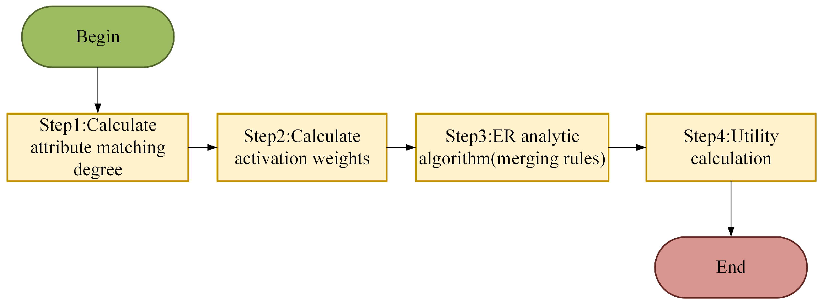
To cope with the rule explosion problem, we use the ER algorithm to fuse the relevant attributes and use the fused data as the premise attributes to construct the corresponding belief rule base. The construction process is shown in Figure 1. The detailed construction process is outlined as follows:

(1)

Determining the attribute match degree:

When premise attribute data are available, Equation (1) is utilized to calculate the match for each attribute reference value. This calculation transforms the match of the premise attribute into a value denoted as $\alpha$. If the match of all premise attributes is non-zero, each attribute has some degree of match, thereby activating the rule.

(2)

Calculate the activation weights:

If the input attribute is available, the belief rule in the classification model is triggered, and the activation weight formula is calculated according to Equation (4) in Section 2.1.

(3)

ER algorithm (merging rules):

After activating the belief rules, the rules are combined and analyzed using the ER algorithm. The ER algorithm is computed according to Equations (5)–(7) in Section 2.1.

(4)

Utility calculation

The classification utility of the Industrial Internet system is calculated using “(8)”, and the evaluation indexes are set according to expert knowledge.

Step 7: Parameter Optimization:

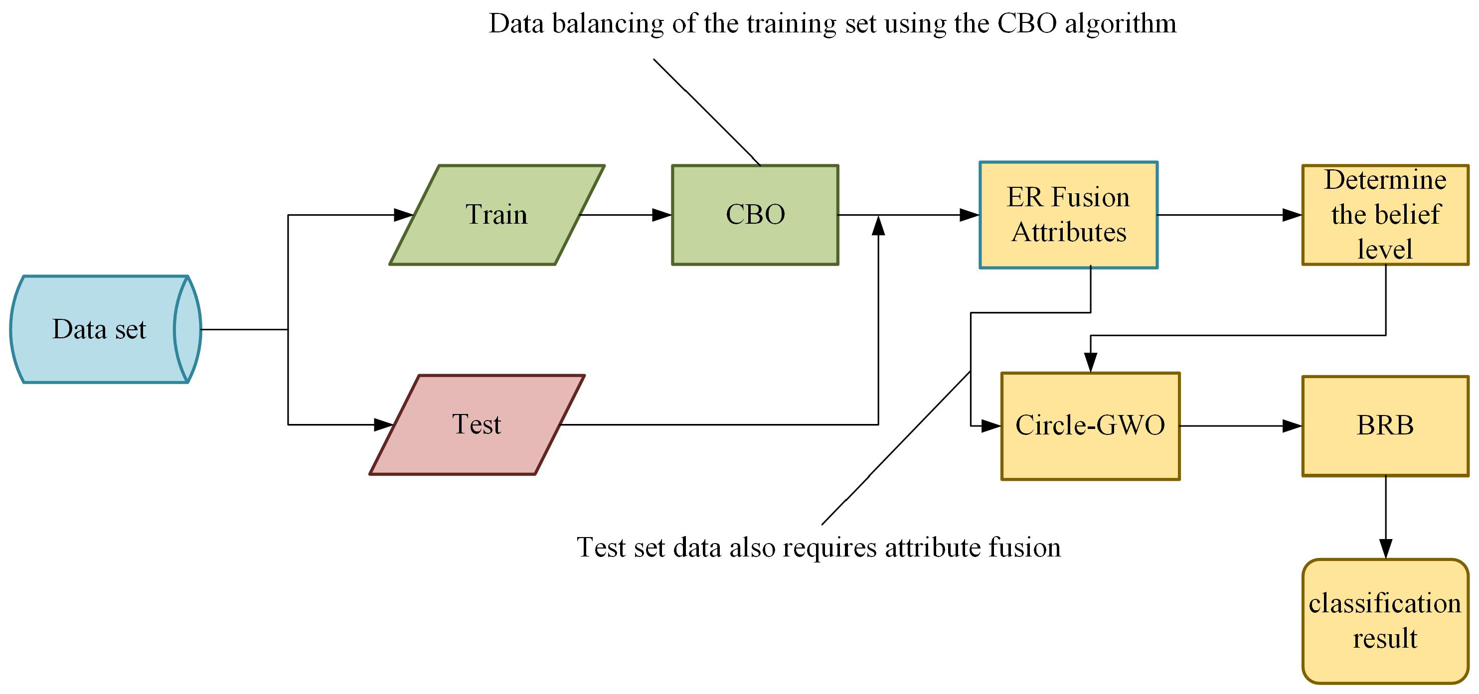
In order to deal with the uncertainty of expert knowledge, the Circle-GWO algorithm is used to optimize the parameters of the BRB model, and the specific model construction and optimization details can be found in Figure 2.

The core functional modules and collaborative logic of the CG-BRB model illustrated in the workflow in Figure 2 are described as follows:

• Data Partitioning and Imbalanced Training-Set Correction: First, the original dataset is divided into a training set and a test set. To address the class-imbalance issue of the training set, the CBO module first performs K-means clustering on the minority-class samples, then synthesizes samples directionally based on the clustering centers. This achieves quantity balance between majority- and minority-class samples, thereby mitigating the negative impact of data imbalance on the model’s classification performance.
• Attribute Fusion and Rule Explosion Mitigation: The number of rules in a BRB follows the formula of $L=m^n$, where n denotes the number of antecedent attributes and m represents the number of reference values for each attribute. The ER attribute fusion operation is performed on the features of both the training set and the test set, fusing them into a small number of comprehensive features through the evidence reasoning algorithm. This reduces the number of antecedent attributes of the BRB; avoids the “rule explosion” problem, where the number of rules grows exponentially with the increase in attributes; and ensures the reasoning efficiency of the BRB.
• Reasoning and Parameter Optimization: The comprehensive features obtained through ER fusion are mapped to the antecedent attributes of the BRB and input into the model, triggering the belief rule-based reasoning process of the BRB. Meanwhile, the Circle-GWO algorithm is adopted to optimize key parameters of the BRB, such as rule confidence degrees and antecedent attribute weights, in order to improve the classification accuracy and convergence stability of the model.

3.2. Circle-GWO Algorithm

Given the complexity of real-world Industrial Internet systems and the impact of environmental disturbances, experts may not be able to provide completely accurate information about the system, leading to uncertainty in expert knowledge. To cope with this uncertainty, the Circle-GWO algorithm is adopted to construct the optimization model. Based on the BRB method, this optimization model aims to enhance the classification accuracy of Industrial Internet cybersecurity data.

(1)

Circle chaotic mapping:

Circle chaotic mapping has some adaptive properties. In this paper, it is used to initialize the gray wolf population, enhancing the diversity of initial BRB parameters. It can be adjusted according to different parameters to adapt to different scenarios, and it can also be adjusted to control its degree of chaos to produce different dynamic behaviors, which is conducive to improving the accuracy of the Gray Wolf optimization algorithm. Its equation is expressed as follows:

$$x_{i+1}=mod\left(d_1{x}_i+d_2-\left({\displaystyle \frac{d_3}{d_1\pi }}\right)sin\left(d_1\pi x_i\right),1\right)$$

(15)

where $d_1$, $d_2$ and $d_3$ are constants and the effect of chaotic mapping can be changed by adjusting their values.

(2)

GWO:

In the GWO algorithm, there is a strict hierarchy within the gray wolf pack. Gray wolf groups are generally divided into four hierarchies—$\alpha$, $\beta$, $\delta$, and $\omega$ (in descending order of authority)—to simulate leadership. The optimization process is described as follows.

Social hierarchy: The $\alpha$ layer is the leader of the whole population, responsible for leading the whole pack to hunt prey, i.e., the optimal solution of the algorithm. The $\beta$ layer is responsible for assisting the $\alpha$ layer, i.e., the sub-optimal solution of the algorithm. The $\delta$ layer listens to the commands and decisions made by $\alpha$ and $\beta$. Poorly adapted individuals (originally $\alpha$ and $\beta$) will fall to the $\delta$ layer. The $\omega$ layer follows the position of $\alpha$, $\beta$ or $\delta$. In the context of BRB parameter optimization, the position vector of each gray wolf corresponds to a set of candidate parameters including rule weights (${\eta }_k$), attribute weights (${\xi }_i$) and belief levels (${\phi }_{n,k}$). Specifically, the $\alpha$ wolf represents the current optimal BRB parameter combination, while $\beta$ and $\delta$ represent the second and third best parameter combinations respectively.

Surrounding Prey: Gray wolf packs surround their prey by following a few equations:

The formula representing the distance between an individual and its prey:

$$\overrightarrow{G}=|\overrightarrow{S}·\overrightarrow{Y_p}\left(t\right)-\overrightarrow{Y}\left(t\right)|$$

(16)

Gray wolf location update equation:

$$\overrightarrow{Y}(t+1)=\overrightarrow{Y_p}\left(t\right)-\overrightarrow{M}\overrightarrow{G}$$

(17)

This process corresponds to the moving of a candidate BRB parameter set towards the current optimal parameters.

The coefficient vector:

$$\overrightarrow{M}=2\overrightarrow{\overline{m}}·\overrightarrow{r1}-\overrightarrow{\overline{m}}$$

(18)

$$\overrightarrow{S}=2·\overrightarrow{r2}$$

(19)

where t denotes the number of iterations of the proposed algorithm; G is the distance between the individual wolf and the prey, which is a vector; $Y_p$ is the prey position vector; and Y is the gray wolf position vector. $\overrightarrow{\overline{m}}$ is the convergence factor, which is a key parameter for balancing GWO exploration and exploitation capabilities. $r1$ and $r2$ are random vectors with elements sampled uniformly from the interval of [0, 1]. $\overrightarrow{S}$ is a search coefficient in the GWO algorithm that is a vector of random values over the interval of [0, 2], and this coefficient gives random weight to the prey so that the GWO algorithm exhibits random search characteristics in the optimization process, which helps to avoid falling into the local optimal solution. Here, “prey” refers to the global optimal parameter combination that minimizes the BRB classification loss function, and the surrounding process corresponds to the initial exploration of the high-dimensional BRB parameter space.

Hunting: Gray wolves have the ability to recognize and round up prey. The mathematical model of an individual gray wolf tracking the location of prey is expressed as follows:

$$\left\{\begin{array}{c}{\overrightarrow{G}}_{\alpha }=|{\overrightarrow{S}}_1·{\overrightarrow{Y}}_{\alpha }-\overrightarrow{Y}|\hfill \\ {\overrightarrow{G}}_{\beta }=|{\overrightarrow{S}}_2·{\overrightarrow{Y}}_{\beta }-\overrightarrow{Y}|\hfill \\ {\overrightarrow{G}}_{\delta }=|{\overrightarrow{S}}_3·{\overrightarrow{Y}}_{\delta }-\overrightarrow{Y}|\hfill \end{array}\right.$$

(20)

where $G_{\alpha }$, $G_{\beta }$, and $G_{\delta }$ denote the distances between $\alpha$, $\beta$, and $\delta$ and other individuals; $Y_{\alpha }$, $Y_{\beta }$, and $Y_{\delta }$ denote the current positions of $\alpha$, $\beta$, and $\delta$ respectively; ${\overrightarrow{S}}_1$, ${\overrightarrow{S}}_2$, and ${\overrightarrow{S}}_3$ are random vectors; and Y is the current position of the gray wolf.

The equation for updating the positions of individual gray wolves is expressed as follows:

$$\left\{\begin{array}{c}{\overrightarrow{Y}}_1={\overrightarrow{Y}}_{\alpha }-{\overrightarrow{M}}_1·\left({\overrightarrow{G}}_{\alpha }\right)\hfill \\ {\overrightarrow{Y}}_2={\overrightarrow{Y}}_{\beta }-{\overrightarrow{M}}_2·\left({\overrightarrow{G}}_{\beta }\right)\hfill \\ {\overrightarrow{Y}}_3={\overrightarrow{Y}}_{\delta }-{\overrightarrow{M}}_3·\left({\overrightarrow{G}}_{\delta }\right)\hfill \end{array}\right.$$

(21)

where $Y_1$, $Y_2$, and $Y_3$ denote the positions of $\omega$ adjusted by the influences of $\alpha$, $\beta$, and $\delta$ respectively. The final position is obtained by averaging these three adjusted positions:

$$\overrightarrow{Y}(t+1)={\displaystyle \frac{{\overrightarrow{Y}}_1+{\overrightarrow{Y}}_2+{\overrightarrow{Y}}_3}{3}}$$

(22)

By jointly utilizing the three leading wolves ($\alpha$, $\beta$, and $\delta$), the BRB parameters are searched in multiple directions, preventing premature convergence to local optima.

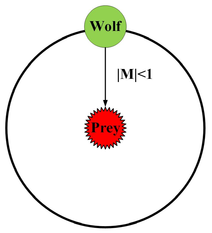
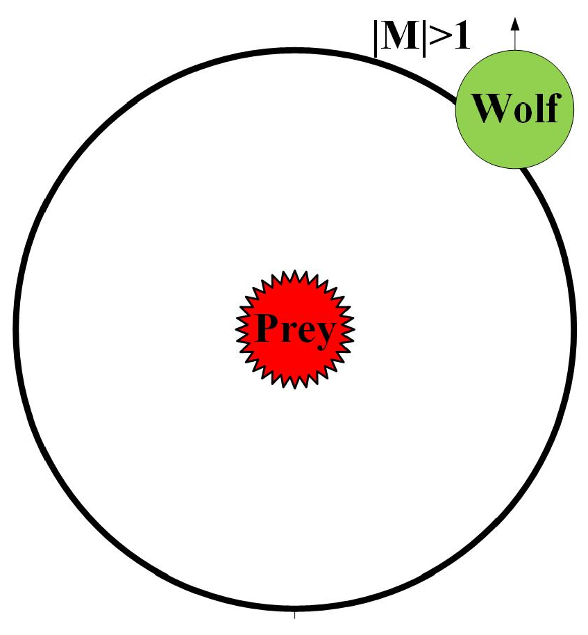
Attacking prey: In the Gray Wolf optimization algorithm, when the prey stops moving, the gray wolves will complete the hunting process by attacking. In order to simulate the process of approaching the prey, a parameter ($\overrightarrow{\overline{m}}$) is introduced, whose value will continuously shrink so that the fluctuation range of $\overrightarrow{M}$ will gradually decrease. In other words, during the iteration of the optimization, when a parameter (a) is linearly contracted from an initial value of 2 to a final value of 0, the value of the corresponding $\overrightarrow{M}$ will also change in the interval of $[-m,m]$. A smaller value of “m” means that the gray wolf is closer to the target prey and is more inclined to search locally ($\left|M\right|<1$), as shown in Figure 3. However, a large value of “m” means that the gray wolf is farther away from the target prey and is more inclined to search globally ($\left|M\right|>1$), as shown in Figure 4. This relationship is given by the following equation.

$$\overline{m}=2-{\displaystyle \frac{2t}{T}}$$

(23)

where the value of m depends on the current number of iterations (t), as well as the total number of iterations (T). For BRB parameter optimization, this means that the algorithm focuses on global search in the early iterations to cover diverse parameter combinations and shifts to local fine-tuning in the later iterations to refine the optimal parameters near the convergence point.

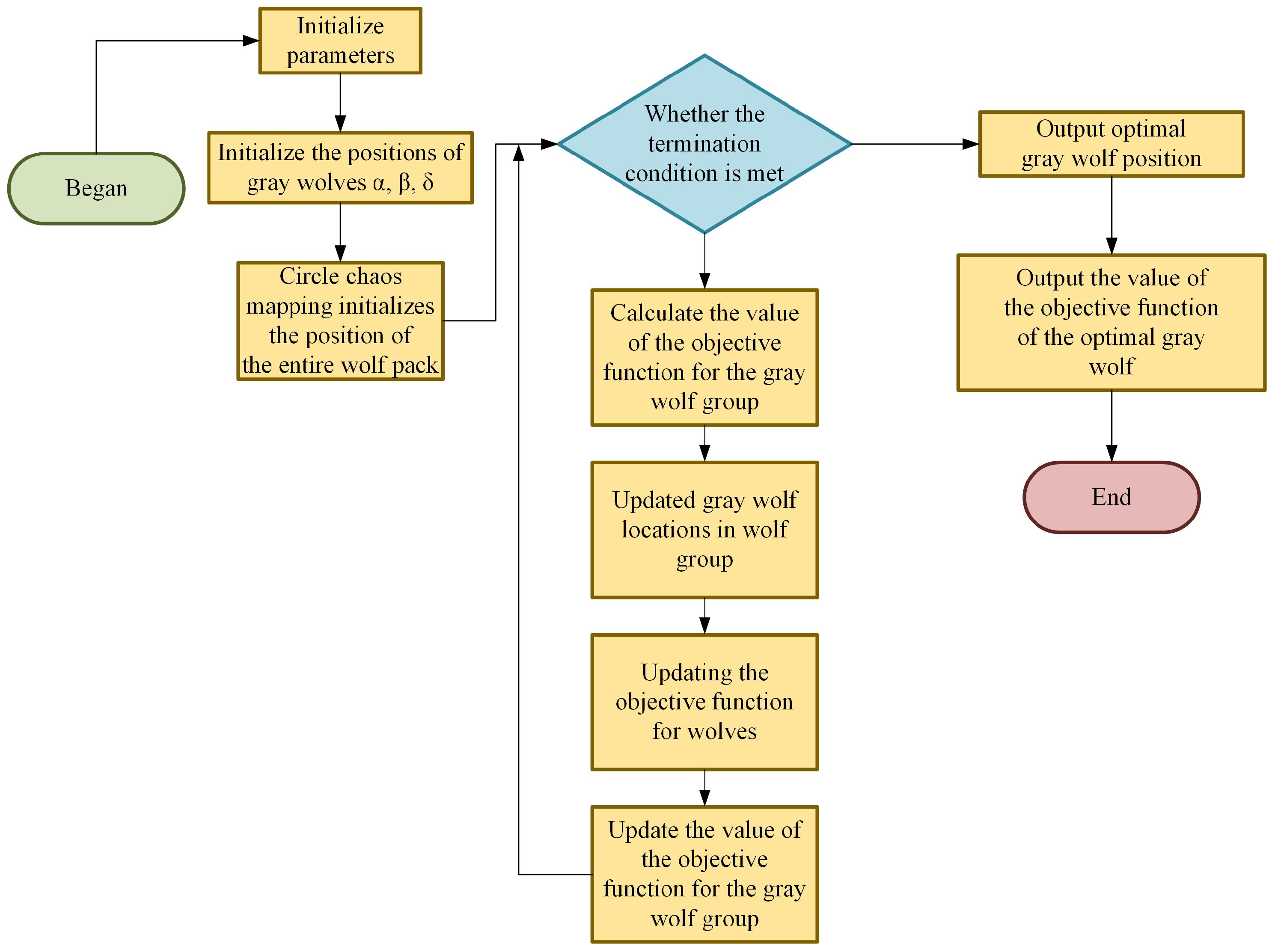
The process of the Circle-GWO algorithm is shown in Figure 5:

4. Case Study

The datasets used in the experiments of this section are derived from the core subsets of the UNSW-NB15 and TON_IoT datasets. Based on the aforementioned datasets, this paper conducts targeted modeling experiments designed to validate the performance differences and statistical significance of different models, as well as to further explore the models’ generalizability. On the UNSW-NB15 dataset, one training set and ten test sets are constructed through random sampling, and ten groups of independent experiments are carried out to ensure the reliability of the verification results. Each training set and test set contains 1100 samples with a data imbalance ratio of 10:1. This setup is used to evaluate the performance of the models in data-imbalanced scenarios. To verify the models’ generalizability, extended experiments are conducted on the TON_IoT dataset. Two data imbalance ratios (5:1 and 10:1) are set via random sampling, with specific experimental parameters as follows: when the imbalance ratio is 5:1, the training and test sets each contain 600 samples; when it is 10:1, both sets contain 1100 samples.

4.1. Optimal Feature Subset Selection

The raw network packets of the UNSW-NB15 dataset were created by the IXIA PerfectStorm tool in the Cyber Range Lab of UNSW Canberra for the generation of a hybrid of real modern normal activities and synthetic contemporary attack behaviors. There are a total of 49 features categorized into 6 major types. Among them, there are many irrelevant and redundant features. An excessive number of features will cause the rule explosion problem in the BRB and, to a certain extent, reduce the performance of the algorithm and the classifier.

Moustafa and Slay [36] used association rule-mining techniques in their study to select the best features for the UNSW-NB15 dataset. Then, in 2017, T. Janarthanan et al. [37] went further and applied a variety of feature selection methods to the UNSW-NB15 dataset, including the CfsSubsetEval method, GreedyStepwise method, InfoGainAttributeEval method and Ranker method. They evaluated the features recommended by these methods and ran machine learning algorithms such as random forests in Weka. The experimental results show that the five features shown in Figure 6 perform the best among the proposed feature subsets.

Among them, the service (e.g., fttp, ftp, dns, and other nominal features; see

Table 1. Numerical encoding mapping of service-type nominal features.

Numerical Service
style	numerical	style	numerical	style	numerical
- (no service)	0	Dhcp	1	dns	2
ftp	3	ftp–data	4	http	5
Irc	6	Pop3	7	radius	8
Smtp	9	Snmp	10	ssh	11
Ssl	12

for numerical values), sbytes (source-to-target bytes), and sttl (source-to-target survival time) features belong to the base feature class. The smean feature (the mean value of the size of the stream packets transmitted by src) belongs to the content feature class, and the ct_dst_sport_ltm feature (records with the same source IP address and source port number in one hundred records according to the last time of the record) belongs to the additional generated feature class.

The TON_IoT dataset contains heterogeneous data including telemetry, operating system logs, and network traffic, covering both normal behaviors and various attacks (e.g., DoS, DDoS, and ransomware) targeting IoT/IIoT services. It supports the training and performance evaluation of intrusion detection systems and security situation assessment models.

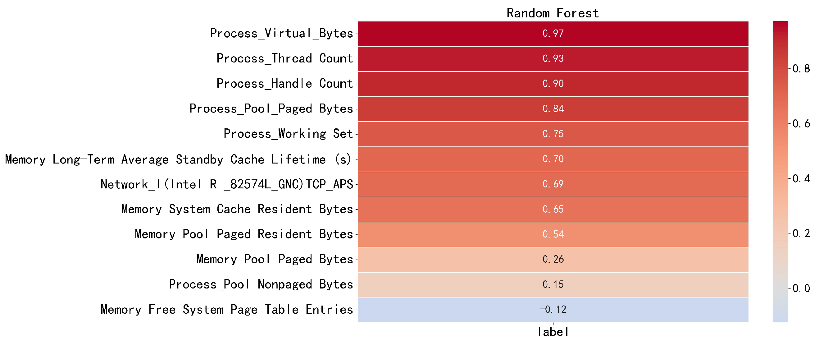
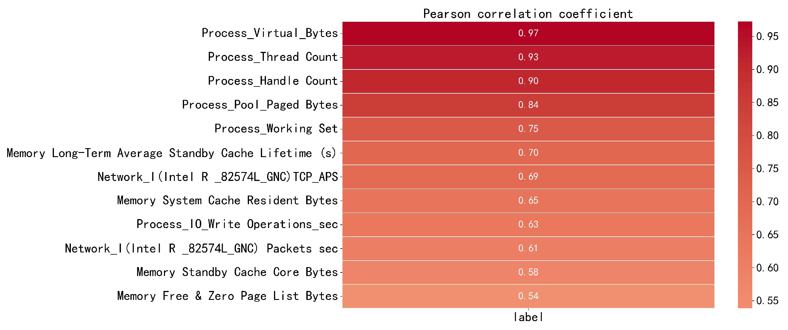
To screen out the feature subset with the highest degree of correlation with the target label, this study employs two classic feature selection methods: the Random Forest algorithm based on decision tree integration and the Pearson correlation coefficient method based on statistical correlation. The former evaluates the importance of features by calculating the splitting gain of features in the tree model, while the latter quantifies the linear correlation degree between features and the label. These two methods construct the feature evaluation system from two dimensions (model-driven and statistical correlation, respectively). By integrating the evaluation results of the two methods, it not only retains the features with statistical significance but also ensures the actual contribution of the selected features to the model prediction. Eventually, a feature subset with a high degree of correlation with the target label and a low redundancy level is constructed, which significantly improves the prediction performance and generalization ability of the model. The results of feature selection using the Random Forest algorithm and the Pearson coefficient are shown in Figure 7 and Figure 8 respectively.

Through the comprehensive analysis of the Random Forest algorithm and the Pearson correlation coefficient, we selected the following four features that have the strongest correlation with the labels:

• Process_Virtual_Bytes Peak: Represents the peak value of the virtual bytes of a process, reflecting the maximum amount of virtual memory used by the process during its operation;
• Process_Thread Count: Represents the number of threads of a process, reflecting the concurrent processing capability of the process;
• Process_Handle Count: Represents the number of handles of a process, reflecting the occupancy of system resources by the process;
• Process_Pool_Paged Bytes: Represents the number of bytes in the paged pool of the process, reflecting the usage of paged memory by the process.

4.2. Problem Description

The purpose of this case study was to demonstrate the validity of the proposed classification method, in which the experiment was conducted for the imbalance problem, in which the class with fewer samples was denoted as positive, i.e., positive samples, and the class with more samples was denoted as negative, i.e., negative samples.

(1)

Establishment of cybersecurity data classification model for Industrial Internet based on CG-BRB

Step 1: Setting the reference values for the BRB model ${\mu }_i$:

There are 10 classes in this dataset:

$\{m_1,m_2,m_3,m_4,m_5,m_6,m_7,m_8,m_9,m_{10}\}$ = {Normal, Analysis, Backdoor, Dos, Exploits, Fuzzers, Reconnaissance, Generic, Shellcode, Worms}. According to the dataset labels and cybersecurity semantics, these ten classes are mapped into two security states: normal data and attack data. Specifically, Normal is defined as normal data, while {Analysis, Backdoor, Dos, Exploits, Fuzzers, Reconnaissance, Generic, Shellcode, Worms} are defined as attack data, that is ${\mu }_i=\{0,1\}$, where ${\mu }_0=0$ is normal data and ${\mu }_1=1$ is attack data.

Step 2: Rebalancing of training-set data:

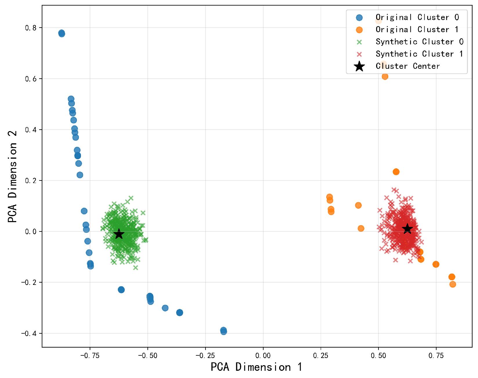
The CBO algorithm is employed to rebalance the training set. The specific implementation procedure is described as follows: First, the minority-class samples are partitioned into several clusters using K-means clustering, where the number of clusters is determined by the elbow method. Subsequently, based on the inherent class-imbalance ratio, synthetic data are generated at the centroid of each cluster to transition the dataset into a balanced state. The evaluation of synthetic data quality remains a complex challenge due to the lack of standardized, widely accepted criteria [38]. To comprehensively assess the quality of our generated synthetic data, we adopt both theoretical and experimental approaches. Theoretically, we use widely accepted metrics to evaluate the consistency between synthetic and original data. Experimentally, we conduct a controlled study using logistic regression: the majority-class samples and the test set remain unchanged, while the minority-class samples in the training set are replaced with either original or synthetic samples. The resulting classification performances are then compared to isolate the impact of synthetic data quality on model behavior. To verify the effectiveness of the CBO oversampling method in preserving the original data structure, we performed an adaptive clustering analysis (based on the elbow method) on the minority-class samples. As illustrated in Figure 9, the original 100 minority-class samples were adaptively partitioned into two clusters via the K-means algorithm, with the distribution as follows: Cluster 0 contains 47 samples (47.0%), and Cluster 1 contains 53 samples (53.0%).

Figure 9 illustrates the distribution of original minority-class samples and CBO-generated samples in the PCA dimension-reduced space. After reducing the five-dimensional features to two dimensions via principal component analysis, we visually observed the following key characteristics:

Cluster structure preservation: The distribution patterns of the original Cluster 0 and Cluster 1 are effectively retained in the synthetic samples. Synthetic samples are tightly clustered around the original clusters, with no significant structural deviation.

Intra-cluster compactness: Synthetic and original samples within each cluster exhibit high aggregation in the PCA space, indicating that the generation process preserves the compactness of the original clusters. The centroids of Cluster 0 and Cluster 1 remain relatively stable, with no substantial shifts induced by synthetic samples.

Inter-cluster separability: The two clusters maintain a distinct separation boundary in the PCA space, with no cross-cluster mixing of synthetic samples. This verifies that the CBO method can retain the discriminative features between original clusters, avoiding the blurring of class boundaries caused by oversampling.

Following the comprehensive evaluation framework for synthetic data introduced by Hernandez et al. [39], the quality of the generated synthetic data was assessed across multiple dimensions. The corresponding results are summarized in

Table 2. Evaluation metrics of CBO oversampling of synthetic data quality.

Evaluation Metric	Score
Silhouette coefficient	0.5925
Diversity	0.7055
Hellinger distance	0.1842
Pairwise correlation difference (PCD)	0.1162
AUC-ROC	0.5867

.

The silhouette coefficient ranges within $[-1, 1]$. A larger value indicates better intra-cluster compactness and inter-cluster separability of samples. Values in the range of 0.71–1.0 correspond to the excellent interval, and 0.51–0.70 is the good interval [40]. The result obtained in this paper is 0.5925, which is in the good interval. This shows that synthetic samples can reasonably preserve the clustering structure of the original data, exhibiting a stable and rational cluster distribution pattern.

Diversity is utilized to measure the discrepancy among generated samples, with a value range of $[0, 1]$. A higher score represents better sample differentiation and effectively avoids simple replication of original data. The diversity score of 0.7055 is at a relatively high level, indicating that the CBO method can effectively prevent invalid sample duplication and reduce the risk of model overfitting.

The Hellinger distance ranges within [0, 1]. A smaller value indicates a closer probability distribution between synthetic samples and original data. The result of 0.1842 in this paper confirms that the overall distribution deviation between synthetic data and original data is extremely small and that the distribution fitting effect is ideal.

The PCD index ranges within [0, 1]. A smaller value represents higher feature restoration accuracy of synthetic minority-class samples. The PCD result of this paper is 0.1162, which illustrates that the features of generated minority-class samples are consistent with real samples and that the sample generation accuracy is high.

AUC-ROC is adopted to measure the ability of classifiers to distinguish real samples from synthetic samples, with a value range of [0.5, 1]. The closer the value is to 0.5, the higher the similarity and the better the fusion effect between the two types of samples. The result of this paper is 0.5867, which proves that synthetic samples are highly similar to real samples in features and difficult to distinguish, with excellent data simulation performance and authenticity.

As shown in

Table 3. Results of Logistic regression on original and synthetic training sets.

Evaluation Metric	Original Minority	Synthetic Minority
Recall	0.8700	0.8900
F1-score	0.9255	0.8900

, compared with training on original minority-class data, training on synthetic data slightly increases recall (0.8700 → 0.8900) while marginally decreasing the F1 score (0.9255 → 0.8900). These minor fluctuations are acceptable, even with a slight gain in minority-class detection. This demonstrates that the synthetic data preserve the key characteristics of the original data and have no significantly different impact on model performance.

Step 3: Data Characterization:

Selected feature subsets are fused. Content and generated features are fused based on shared attributes. Fusion results $x_1$ and $x_2$ serve as BRB premise attributes 1 and 2, with labeled features as the model’s outputs.

Five core attributes—service, sbytes (source bytes), sttl (source time to live), smean (mean source packet size), and ct_dst_sport_ltm (long-term count of connections to the destination port)—are selected for analysis. Firstly, continuous attributes (sbytes, sttl, and smean) are standardized to eliminate dimensional discrepancies. For the discrete “service” attribute, one-hot encoding is applied for numerical transformation. Based on data distribution characteristics and domain knowledge in network security, all attributes are then mapped to belief distributions that include five preset evaluation levels and global ignorance, with each distribution strictly satisfying the non-negativity and normalization constraints of belief measures.

Subsequently, the attributes are divided into two groups according to their network security semantic features: the traffic intensity group (sbytes, smean, and sttl) and the connection anomaly group (service and ct_dst_sport_ltm). The Entropy Weight Method (EWM) is employed to determine the weight of each attribute within its respective group, thereby quantifying the attribute’s information contribution—where lower information entropy indicates stronger discriminative power and a higher corresponding weight.

Based on the calculated weights, the belief distribution of each attribute in the group is discounted to obtain the Basic Probability Assignment (BPA) of the corresponding evidence. The BPAs of all evidence within the group are then fused iteratively. During the fusion process, a normalization conflict factor specific to the Evidential Reasoning (ER) algorithm is introduced to effectively address significant conflicts between pieces of evidence, ensuring the rationality of the fusion result. Ultimately, a comprehensive belief distribution is generated for each group, accurately characterizing the network security state with respect to the dimensions of traffic intensity and connection anomaly.

This ER fusion process achieves effective dimensionality reduction by converting the five original attributes into two comprehensive security indicators. More importantly, it significantly mitigates the rule explosion problem inherent in the Belief Rule Base (BRB) by reducing the number of premise attributes. The number of rules in a BRB follows the formula of $L=m^n$, where n denotes the number of antecedent attributes and m represents the number of reference values for each attribute. Taking the experimental data as an example, if each of the five original attributes contains five reference values, the corresponding number of BRB rules is $5^5=3125$; in contrast, the two reduced-dimension comprehensive attributes (each with five reference values) correspond to only $5^2=25$ rules. This dimensionality reduction scheme substantially lowers model complexity and improves inference efficiency while preserving key security information.

Step 4: BRB Construction:

The results of ER fusion in Step 3, $x_1$,$x_2$ are utilized as prerequisite attributes to construct the BRB model.

Step 5: Parameter optimization:

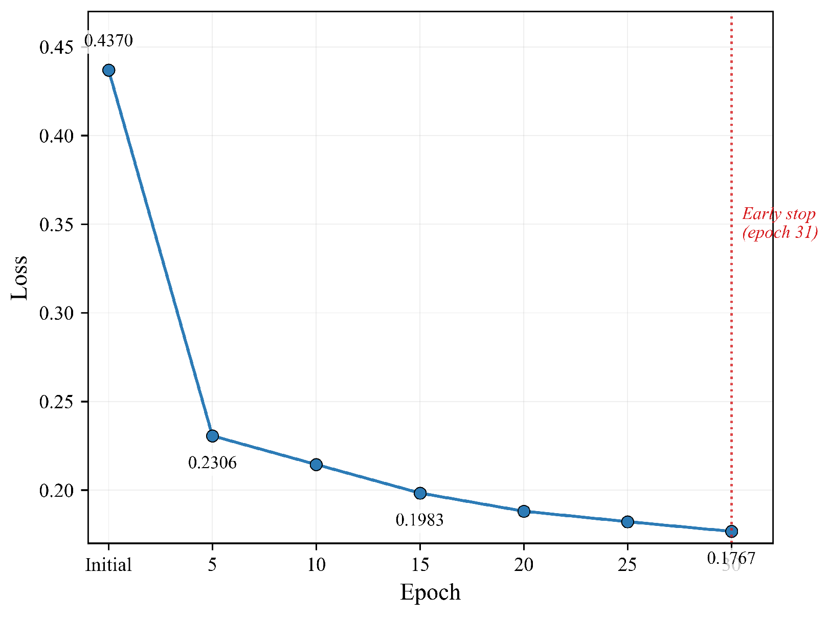
After building the BRB model in Step 4, its parameters are optimized using the Circle-GWO algorithm, and the optimized BRB model is finally generated. An early stopping mechanism is introduced into the optimization process: the optimization will be terminated if there is no improvement in the loss value for five consecutive rounds, with the maximum number of optimization rounds set to 50. The variation between the number of optimization rounds and the loss value is illustrated in Figure 10.

The experimental results before and after optimization are presented in

Table 4. Model Performance Comparison.

Evaluation Metric	Unoptimized BRB	Optimized BRB
Accuracy	0.9573	0.9782
Precision	0.7732	0.8167
Recall	0.7500	0.9800
F1 score	0.7614	0.8909

. The results show that the Circle-GWO algorithm significantly improves both the performance and convergence of the Belief Rule Base (BRB).

(2)

Numerical analysis

For UNSW-NB15, five attributes were selected and divided into 2 categories with imbalance ratios of 5:1 and 10:1. BRB’s prior attribute was set to 2, and Circle-GWO optimized the model for 100 iterations per run. Given data imbalance, accuracy and recall serve as evaluation metrics. The formulas for accuracy, recall, and precision follow:

$$Precision={\displaystyle \frac{TP}{TP+FP}}\ast 100$$

(24)

$$Accuracy={\displaystyle \frac{TP+TN}{TM}}\ast 100$$

(25)

$$Recall={\displaystyle \frac{TP}{TP+FN}}\ast 100$$

(26)

where TM is the number of samples, TP represents the number of positive-class samples correctly predicted as the positive class, FN represents the number of positive-class samples incorrectly predicted as the negative class, and FP represents the number of negative-class samples incorrectly predicted as the positive class.

4.3. Experimental Results and Comparative Studies

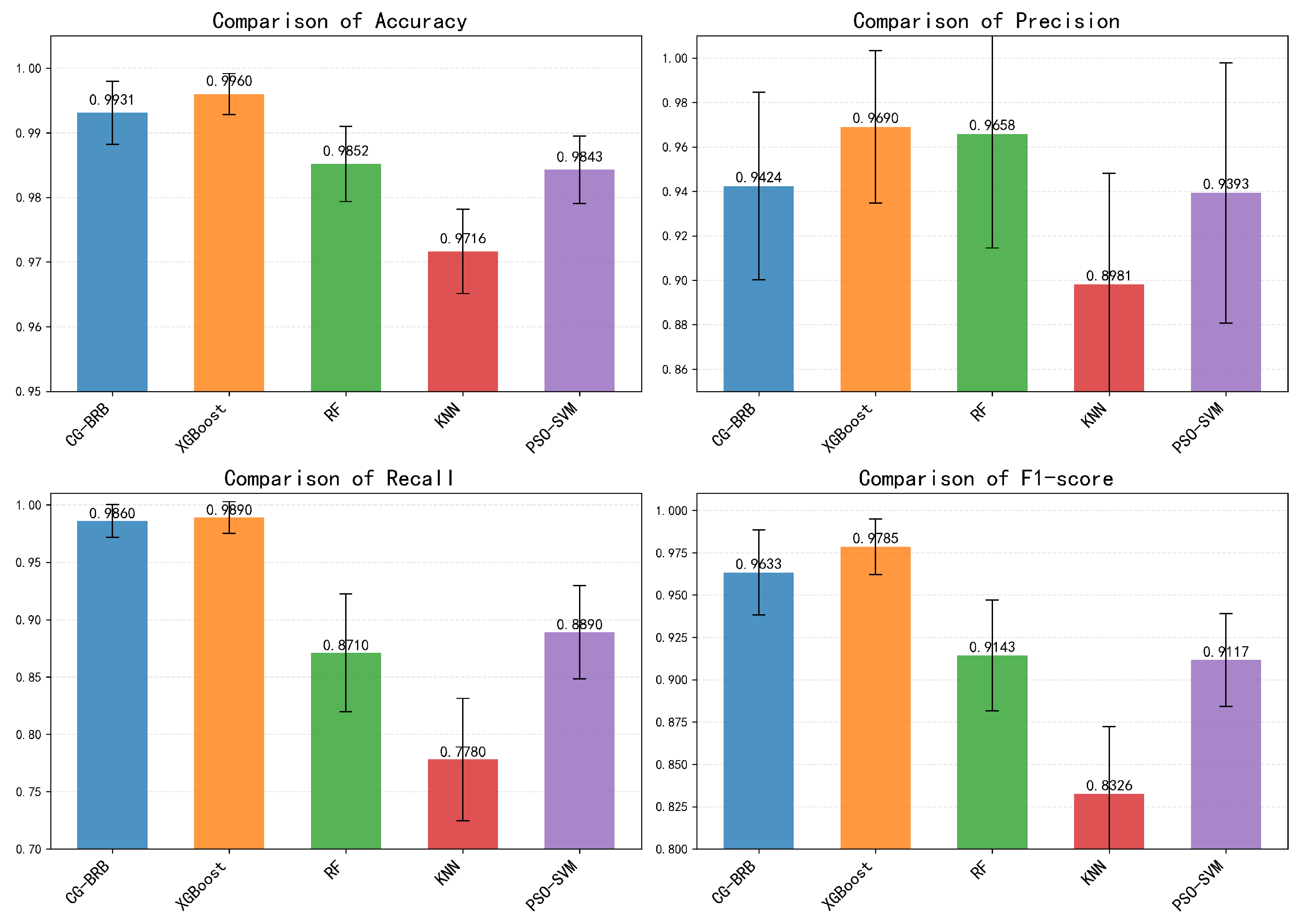
To verify the effectiveness of the proposed CG-BRB model, this paper selects four mainstream classifiers for comparative experiments. These experiments are conducted based on 1100 sample data under the condition of a data imbalance ratio of 10:1, with specific experimental results and comparative analysis presented in

Table 5. Comparison of accuracy among different models.

Classifier	Test 1	Test 2	Test 3	Test 4	Test 5	Test 6
CG-BRB	0.9882	0.9982	0.9936	0.9982	0.9955	0.9945
XGBoost	0.9945	0.9891	0.9936	0.9982	0.9982	0.9964
RF	0.9873	0.9782	0.9918	0.9855	0.9809	0.9836
KNN	0.9773	0.9773	0.9745	0.9682	0.9727	0.9627
PSO-SVM	0.9873	0.9782	0.9818	0.9818	0.9864	0.9882
Classifier	Test 7	Test 8	Test 9	Test 10	Mean	Std
CG-BRB	0.9909	0.9982	0.9900	0.9836	0.9931	0.0046
XGBoost	0.9945	1.0000	0.9982	0.9973	0.9960	0.0033
RF	0.9864	0.9864	0.9764	0.9955	0.9852	0.0058
KNN	0.9636	0.9791	0.9773	0.9636	0.9732	0.0065
PSO-SVM	0.9864	0.9945	0.9791	0.9791	0.9843	0.0054

,

Table 6. Comparison of precision among different models.

Classifier	Test 1	Test 2	Test 3	Test 4	Test 5	Test 6
CG-BRB	0.8991	1.0000	0.9429	0.9804	0.9524	0.9608
XGBoost	0.9434	0.8929	0.9346	0.9900	0.9900	0.9898
RF	0.9479	0.9043	1.0000	0.9884	1.0000	0.9881
KNN	0.8947	0.9213	0.9000	0.8571	0.9730	0.8471
PSO-SVM	0.9388	0.8800	0.9255	0.9878	0.9885	0.9888
Classifier	Test 7	Test 8	Test 9	Test 10	Mean	Std
CG-BRB	0.9412	0.9804	0.9009	0.8661	0.9424	0.0424
XGBoost	0.9796	1.0000	0.9900	0.9802	0.9690	0.0346
RF	1.0000	1.0000	0.8491	0.9798	0.9658	0.0549
KNN	0.8571	0.9873	0.8947	0.8488	0.8981	0.0518
PSO-SVM	0.9775	1.0000	0.8532	0.8532	0.9394	0.0551

,

Table 7. Comparison of recall among different models.

Classifier	Test 1	Test 2	Test 3	Test 4	Test 5	Test 6
CG-BRB	0.9800	0.9800	0.9900	1.0000	1.0000	0.9800
XGBoost	1.0000	1.0000	1.0000	0.9900	0.9900	0.9700
RF	0.9100	0.8500	0.9100	0.8500	0.7900	0.8300
KNN	0.8500	0.8200	0.8100	0.7800	0.7200	0.7200
PSO-SVM	0.9200	0.8800	0.8700	0.8100	0.8600	0.8800
Classifier	Test 7	Test 8	Test 9	Test 10	Mean	Std
CG-BRB	0.9600	1.0000	1.0000	0.9700	0.9860	0.0129
XGBoost	0.9600	1.0000	0.9900	0.9900	0.9890	0.0125
RF	0.8500	0.8500	0.9000	0.9700	0.8710	0.0487
KNN	0.7200	0.7800	0.8500	0.7300	0.7770	0.0460
PSO-SVM	0.8700	0.9400	0.9300	0.9300	0.8890	0.0388

and

Table 8. Comparison of F1 score among different models.

Classifier	Test 1	Test 2	Test 3	Test 4	Test 5	Test 6
CG-BRB	0.9378	0.9899	0.9659	0.9901	0.9756	0.9703
XGBoost	0.9709	0.9434	0.9662	0.9900	0.9900	0.9798
RF	0.9286	0.8763	0.9529	0.9140	0.8827	0.9022
KNN	0.8718	0.8677	0.8526	0.8168	0.8276	0.7784
PSO-SVM	0.9293	0.8800	0.8969	0.8901	0.9198	0.9312
Classifier	Test 7	Test 8	Test 9	Test 10	Mean	Std
CG-BRB	0.9505	0.9901	0.9479	0.9151	0.9633	0.0231
XGBoost	0.9697	1.0000	0.9900	0.9851	0.9785	0.0155
RF	0.9189	0.9189	0.8738	0.9749	0.9143	0.0309
KNN	0.7826	0.8715	0.8718	0.7849	0.8324	0.0365
PSO-SVM	0.9206	0.9691	0.8900	0.8900	0.9117	0.0264

. The selected comparative classifiers include XGBoost, RF, PSO-SVM, and KNN. The mean values and error bars of all experimental results are illustrated in Figure 11 (Error bars denote standard deviation).

In imbalanced classification tasks, accuracy is prone to artificial inflation by majority-class samples, failing to objectively reflect minority-class detection capability. While precision reveals the false-positive risk among minority-class predictions, it overlooks the false-negative risk on true minority samples. In contrast, recall directly quantifies minority-class coverage, serving as the core metric for critical sample identification. As the harmonic mean of precision and recall, the F1 score balances false positives and false negatives to provide a comprehensive measure of overall classification performance. Thus, this study adopts recall and the F1 score as the primary evaluation metrics.

In terms of the stability of recall and the F1 score, the proposed CG-BRB model exhibits performance comparable to that of XGBoost, and both significantly outperform the other comparative models. Specifically, CG-BRB’s recall standard deviation is 0.0129, which is only slightly higher than that of XGBoost (0.0125) and far lower than those of Random Forest (0.0487), KNN (0.0460), and PSO-SVM (0.0388). For the F1 score, the standard deviation of CG-BRB is 0.0231, showing a small gap relative to XGBoost (0.0155) and PSO-SVM (0.0264) while being obviously superior to Random Forest (0.0309) and KNN (0.0365).

To verify whether the CG-BRB model proposed in this paper has statistically significant advantages over other comparative models, this section conducts significance tests on two core evaluation metrics—namely, recall and F1 score. The test procedure first adopts the Shapiro–Wilk test to analyze the normality of the data, on the basis of which the specific method for subsequent significance tests is determined. The results of the Shapiro–Wilk test are presented in

Table 9. Shapiro–Wilk normality test results for recall rate.

Model	W Value	p Value	Comparison with $\mathit{\alpha }=0.05$	Conclusion
CG-BRB	0.9234	0.386	$p>0.05$	Normality
XGBoost	0.9412	0.578	$p>0.05$	Normality
RF	0.9017	0.243	$p>0.05$	Normality
KNN	0.9356	0.498	$p>0.05$	Normality
PSO-SVM	0.9187	0.352	$p>0.05$	Normality

and

Table 10. Shapiro–Wilk normality test results for F1 score.

Model	W Value	p Value	Comparison with $\mathit{\alpha }=0.05$	Conclusion
CG-BRB	0.9083	0.287	p > 0.05	Normality
XGBoost	0.9215	0.365	p > 0.05	Normality
RF	0.9458	0.621	p > 0.05	Normality
KNN	0.9267	0.413	p > 0.05	Normality
PSO-SVM	0.9324	0.457	p > 0.05	Normality

.

The results of the aforementioned Shapiro–Wilk test indicate that the datasets corresponding to the recall and F1 score of each model all conform to the normal distribution. On this basis, this paper adopts the paired t-test method to conduct subsequent significance tests.

• ${\mathbf{H}}_{\mathbf{0}}$: The indicator difference between the CG-BRB model and the comparative models is equal to 0 (i.e., there is no significant difference between them).
• ${\mathbf{H}}_1$: The indicator difference between the CG-BRB model and the comparative models is not equal to 0 (i.e., there is a significant difference between them).
• Significance level $\alpha =0.05$.

The experimental results are presented in

Table 11. Paired t-test results for recall rate.

Comp. Model	Mean Diff.	Std. Dev. of Diff.	t-Statistic
CG-BRB vs. XGBoost	−0.0030	0.0134	−0.709
CG-BRB vs. RF	0.1150	0.0574	6.336
CG-BRB vs. KNN	0.2080	0.0503	13.080
CG-BRB vs. PSO-SVM	0.0970	0.0445	6.896
Comp. Model	df	Two-tailed  p-Value	Significance ($\mathit{\alpha }=\mathbf{0.05}$)
CG-BRB vs. XGBoost	9	$\approx 0.497$	Not Significant
CG-BRB vs. RF	9	<0.001	Highly Significant
CG-BRB vs. KNN	9	<0.0001	Extremely Significant
CG-BRB vs. PSO-SVM	9	<0.001	Highly Significant

and

Table 12. Paired t-test results for F1 score.

Comp. Model	Mean Diff.	Std. Dev. of Diff.	t-Statistic
CG-BRB vs. XGBoost	−0.0152	0.0305	−1.573
CG-BRB vs. RF	0.0490	0.0509	3.043
CG-BRB vs. KNN	0.1308	0.0407	10.150
CG-BRB vs. PSO-SVM	0.0516	0.0337	4.842
Comp. Model	df	Two-Tailed   p-Value	Significance  ($\mathit{\alpha }=\mathbf{0.05}$)
CG-BRB vs. XGBoost	9	$\approx 0.149$	Not Significant
CG-BRB vs. RF	9	$\approx 0.014$	Significant
CG-BRB vs. KNN	9	<0.0001	Extremely Significant
CG-BRB vs. PSO-SVM	9	<0.001	Highly Significant

.

The superiority of the CG-BRB model is fully verified through statistical significance analysis based on 10 independent test datasets. The Shapiro–Wilk normality test confirms that the core performance metrics (recall and F1 score) of all comparative models follow a normal distribution. On this basis, a two-tailed paired t-test with a significance level of $\alpha =0.05$ is adopted to conduct paired difference analysis. The results show that the CG-BRB model exhibits significant or extremely significant advantages over the RF, KNN, and PSO-SVM models in key performance metrics.

In terms of recall, compared with the RF, KNN, and PSO-SVM models, the two-tailed p-values of the CG-BRB model are all less than 0.001, with mean differences reaching 0.115, 0.209, and 0.097, respectively. Among these, the performance gap with the KNN model is the most prominent: the average recall is 20.9% higher, and the corresponding t-statistic is as high as 13.080, which fully demonstrates that the advantage of the CG-BRB model in recall capability has strong statistical reliability. In terms of the F1 score, which characterizes comprehensive performance, compared with the RF, PSO-SVM, and KNN models, the two-tailed p-values of the CG-BRB model are $\approx 0.149$, $<0.001$, and less than 0.0001 (for KNN), respectively, with mean differences of 0.049, 0.0516, and 0.1309 in sequence. This further verifies that the model is significantly superior to the above three models in balancing precision and recall.

To assess the statistical significance of performance differences between CG-BRB and XGBoost, paired two-tailed t-tests were performed on the 10-fold cross-validation results (degrees of freedom, $df=9$; significance level, $\alpha =0.05$). As shown in Table 11 (recall) and Table 12 (F1 score), the two-tailed p-values for the comparisons are approximately 0.497 (recall) and 0.149 (F1 score), both of which exceed the pre-defined significance level of 0.05. Combined with the negligible mean performance differences, these results confirm that there are no statistically significant differences between the two models in core classification performance. Given that XGBoost has been widely proven to achieve excellent performance in imbalanced data classification tasks, this finding further confirms that the CG-BRB model also achieves competitive performance on imbalanced data classification tasks.

However, in Industrial Internet scenarios, operation and maintenance personnel not only require models to accurately identify whether an event is classified as an attack but also demand clear justifications for these decisions and traceable reasoning processes. Traditional machine learning models represented by XGBoost are essentially “black-box models” that cannot provide clear decision-making logic and interpretability for operation and maintenance staff, making it difficult for them to meet the stringent requirements of the Industrial Internet field. In contrast, the CG-BRB model offers inherently strong interpretability, which enables explicit and traceable reasoning processes. Therefore, it is more suitable for the practical application requirements of the Industrial Internet domain.

Overall analysis shows that the CG-BRB model is not only statistically superior to the RF, KNN, and PSO-SVM models but also that it has a unique interpretability advantage while maintaining performance comparable to that of the XGBoost model. It fully meets the dual requirements of model performance and operational security in the Industrial Internet field, making it a better solution for imbalanced data classification tasks in this field.

4.4. Verification of Model Applicability

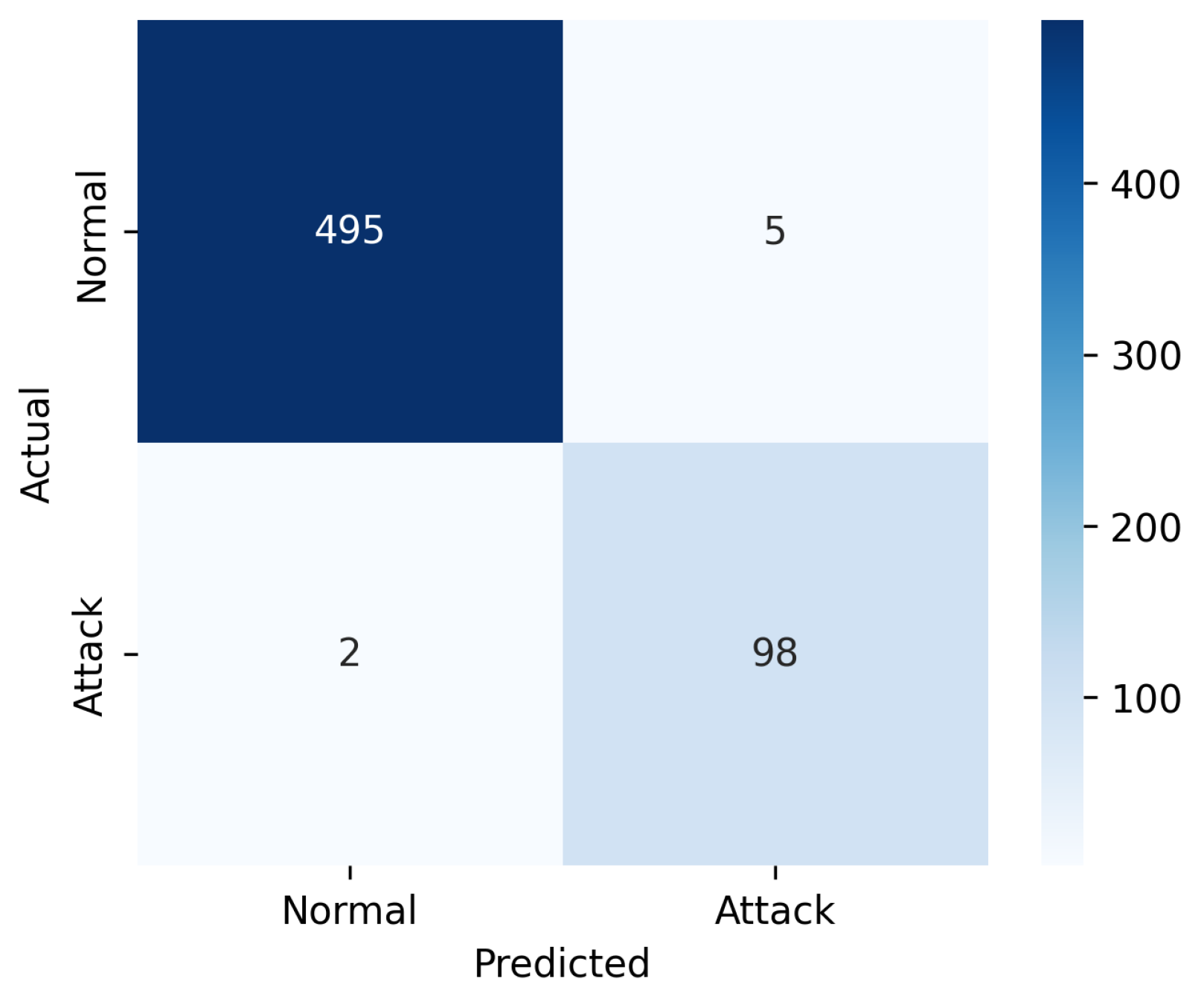
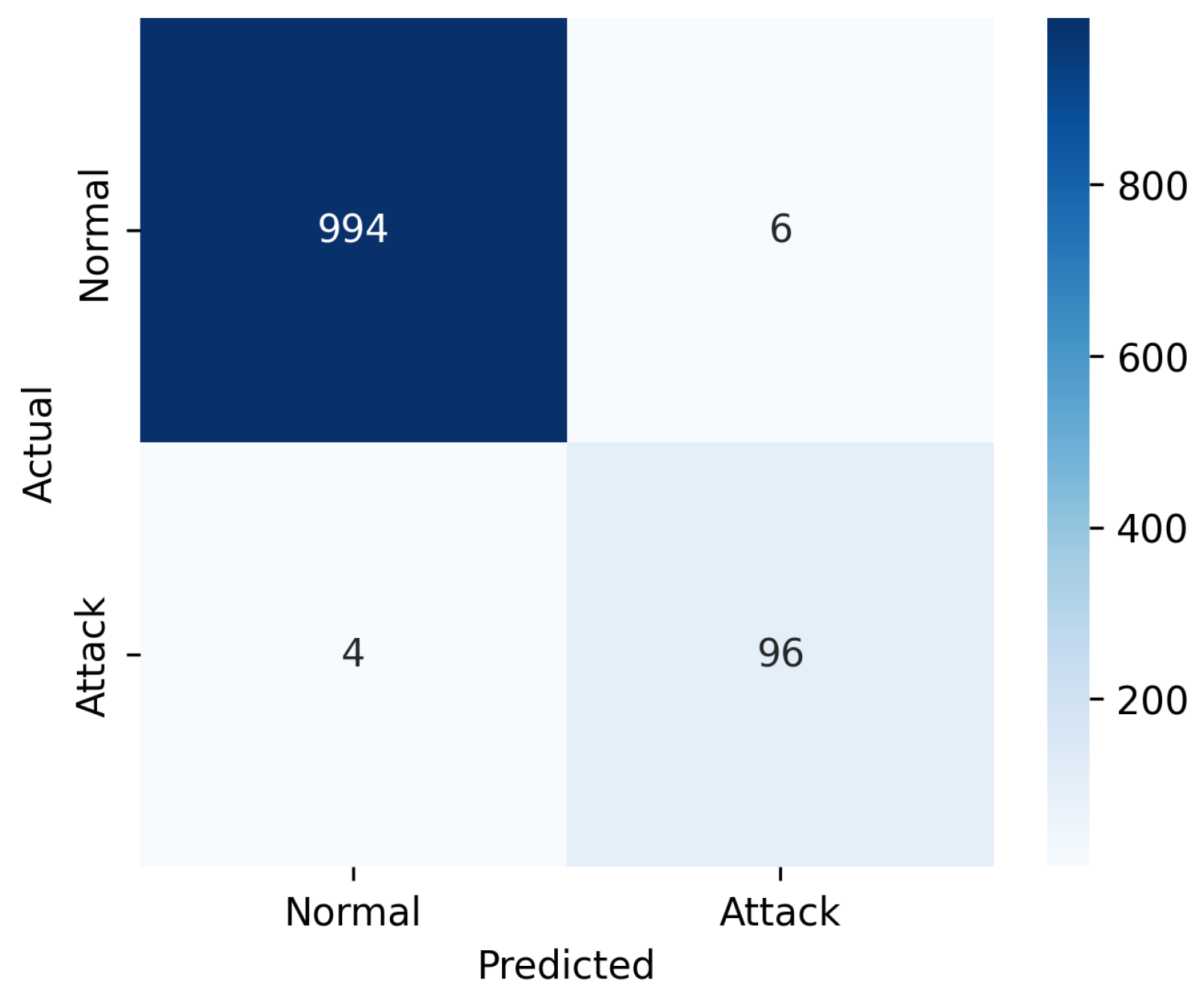
To verify the applicability of the model, we conduct experiments on the TON_IoT dataset, which is a dataset for the new generation of the Internet of Things and Industrial Internet of Things. The dataset is divided into two subsets with imbalance ratios of 5:1 and 10:1. In the subset with an imbalance ratio of 5:1, there are 500 normal data records and 100 attack data records. In the subset with an imbalance ratio of 10:1, there are 1000 normal data records and 100 attack data records. We train and test the model to obtain the accuracy, precision, recall, and F1 score for the two subsets. The experimental results are shown in

Table 13. Model performance under different imbalance ratios.

Imbalance Ratio	Recall	Accuracy	Precision	F1 Score
5:1	98.00	98.83	95.15	96.55
10:1	96.00	99.09	94.12	95.05

and Figure 12 and Figure 13.

This supplementary experiment is conducted based on class-imbalance ratios of 5:1 (corresponding to a dataset size of 600) and 10:1 (corresponding to a dataset size of 1100), aiming to further verify the performance of the model on Industrial Internet-related datasets. When the imbalance ratio increases from 5:1 to 10:1, the model’s recall slightly decreases from 98.00 to 96.00 yet remains at a high level of 96%. This indicates that even as the proportion of minority-class samples shrinks, the model’s ability to identify the core-focused minority-class samples does not exhibit significant attenuation, demonstrating its good robustness against variations in data imbalance levels. Meanwhile, the accuracy slightly rises from 98.83 to 99.09, which suggests that the model’s classification performance for majority-class samples becomes more stable as the proportion of majority-class samples increases. The precision slightly drops from 95.15 to 94.12, which is a reasonable outcome reflecting the slight increase in misjudgment risk for minority-class samples when the class-imbalance level intensifies, and the overall fluctuation range is controllable. As a comprehensive evaluation metric integrating precision and recall, the F1 score gently decreases from 96.55 to 95.05. Considering that the 10:1 imbalance ratio corresponds to a larger dataset size, the model can still maintain a high level of comprehensive classification performance of over 95% under the dual conditions of expanded dataset size and intensified imbalance level. In summary, this experiment further verifies that the model has strong applicability and stability on Industrial Internet-related data, as it not only ensures a high recognition rate for core minority-class samples but also maintains excellent overall classification performance.

5. Conclusions

This paper addresses the class-imbalance problem in Industrial Internet cybersecurity by constructing the CG-BRB classification model. Experimental results show that the proposed model significantly outperforms traditional machine learning methods such as Random Forest and KNN on imbalanced data classification tasks and achieves competitive performance compared with the state-of-the-art XGBoost model. Compared with black-box machine learning models, CG-BRB provides traceable rule-based reasoning and inherent interpretability, making it better suited for practical Industrial Internet operation and maintenance scenarios that require transparent and traceable decision-making processes.

Nevertheless, the proposed model still has certain limitations. The construction of initial rules and belief degrees relies on manually defined expert knowledge, which restricts the model’s adaptability to emerging and unknown cyberattacks. In addition, this work focuses exclusively on binary classification tasks. Future work will aim to reduce dependence on expert knowledge by developing a data-driven automatic rule generation mechanism, thereby improving the model’s dynamic adaptability. Furthermore, the model will be extended to handle multi-class imbalanced network attack classification tasks.

References

1. Wei, Z.; Sun, S.; Masouros, C.; Wang, J.; Hu, R.Q.; Adachi, F. Guest editorial special issue on current research trends and open challenges for industrial internet of things. IEEE Internet Things J. 2024, 11, 26548–26551. [Google Scholar] [CrossRef]
2. Rajasekaran, V.A.; Indirajithu, A.; Jayalakshmi, P.; Nayyar, A.; Balusamy, B. Gradient scaling and segmented SoftMax regression federated learning (GDS-SRFFL): A novel methodology for attack detection in industrial internet of things (IIoT) networks. J. Supercomput. 2024, 80, 16860–16886. [Google Scholar] [CrossRef]
3. Korsvik, V.P.I. Cyber Security Risk Perception and Mitigation Strategies Within the Maritime Shipping Industry. Ph.D. Thesis, University of South-Eastern Norway, Notodden, Norway, 2023. [Google Scholar]
4. Liao, Y.; Li, M.; Sun, Q.; Li, P. Advanced stacking models for machine fault diagnosis with ensemble trees and SVM. Appl. Intell. 2025, 55, 251. [Google Scholar] [CrossRef]
5. Dong, S. Multi-class SVM algorithm with active learning for network traffic classification. Expert Syst. Appl. 2021, 176, 114885. [Google Scholar] [CrossRef]
6. Zhang, S. Cost-sensitive KNN classification. Neurocomputing 2020, 391, 234–242. [Google Scholar] [CrossRef]
7. Bing, W.; Xiong, H. Fault diagnosis technique based on multi-domain features and RelifF-Bayes-KNN in rolling bearing. Nonlinear Dyn. 2025, 113, 12985–13000. [Google Scholar] [CrossRef]
8. Aitkenhead, M.J. A co-evolving decision tree classification method. Expert Syst. Appl. 2008, 34, 18–25. [Google Scholar] [CrossRef]
9. Nancy, P.; Muthurajkumar, S.; Ganapathy, S.; Kumar, S.S.; Selvi, M.; Arputharaj, K. Intrusion detection using dynamic feature selection and fuzzy temporal decision tree classification for wireless sensor networks. IET Commun. 2020, 14, 888–895. [Google Scholar] [CrossRef]
10. Vinayakumar, R.; Soman, K.P.; Poornachandran, P. Applying convolutional neural network for network intrusion detection. In 2017 International Conference on Advances in Computing, Communications and Informatics (ICACCI); IEEE: New York, NY, USA, 2017; pp. 1222–1228. [Google Scholar]
11. Yin, C.; Zhu, Y.; Fei, J.; He, X. A deep learning approach for intrusion detection using recurrent neural networks. IEEE Access 2017, 5, 21954–21961. [Google Scholar] [CrossRef]
12. He, H.; Garcia, E.A. Learning from imbalanced data. IEEE Trans. Knowl. Data Eng. 2009, 21, 1263–1284. [Google Scholar] [CrossRef]
13. Lomax, S.; Vadera, S. A survey of cost-sensitive decision tree induction algorithms. ACM Comput. Surv. 2013, 45, 1–35. [Google Scholar] [CrossRef]
14. Zhou, Z.H.; Liu, X.Y. Training cost-sensitive neural networks with methods addressing the class imbalance problem. IEEE Trans. Knowl. Data Eng. 2005, 18, 63–77. [Google Scholar] [CrossRef]
15. Liaw, L.C.M.; Tan, S.C.; Goh, P.Y.; Lim, C.P. A histogram SMOTE-based sampling algorithm with incremental learning for imbalanced data classification. Inf. Sci. 2025, 686, 121193. [Google Scholar] [CrossRef]
16. Han, H.; Wang, W.Y.; Mao, B.H. Borderline-SMOTE: A new over-sampling method in imbalanced data sets learning. In Proceedings of the International Conference on Intelligent Computing; Springer: Berlin/Heidelberg, Germany, 2005; pp. 878–887. [Google Scholar]
17. He, H.; Bai, Y.; Garcia, E.A.; Li, S. ADASYN: Adaptive synthetic sampling approach for imbalanced learning. In 2008 IEEE International Joint Conference on Neural Networks (IJCNN), Hong Kong, China, 1–6 June 2008; IEEE: New York, NY, USA, 2008; pp. 1322–1328. [Google Scholar]
18. Nikpour, B.; Rahmati, F.; Mirzaei, B.; Nezamabadi-Pour, H. A comprehensive review on data-level methods for imbalanced data classification. Expert Syst. Appl. 2026, 295, 128920. [Google Scholar] [CrossRef]
19. Arafa, A.; El-Fishawy, N.A.; Badawy, M.A.; Radad, M. Rn-smote: Reduced noise smote based on dbscan for enhancing imbalanced data classification. J. King Saud Univ. Comput. Inf. Sci. 2022, 34, 5059–5074. [Google Scholar] [CrossRef]
20. Dixit, A.; Mani, A. Sampling technique for noisy and borderline examples problem in imbalanced classification. Appl. Soft Comput. 2023, 142, 110361. [Google Scholar] [CrossRef]
21. Georgios, D.; Fernando, B.; Felix, L. Improving imbalanced learning through a heuristic oversampling method based on k-means and smote. Inf. Sci. 2018, 465, 1–20. [Google Scholar] [CrossRef]
22. Farshidvard, A.; Hooshmand, F.; MirHassani, S.A. A novel two-phase clustering-based under-sampling method for imbalanced classification problems. Expert Syst. Appl. 2023, 213, 119003. [Google Scholar] [CrossRef]
23. Yang, J.B.; Liu, J.; Wang, J.; Sii, H.S.; Wang, H.W. Belief rule-base inference methodology using the evidential reasoning approach—RIMER. IEEE Trans. Syst. Man Cybern. A 2006, 36, 266–285. [Google Scholar] [CrossRef]
24. Yang, L.H.; Liu, J.; Wang, Y.M.; Martínez, L. Extended belief-rule-based system with new activation rule determination and weight calculation for classification problems. Appl. Soft Comput. 2018, 72, 261–272. [Google Scholar] [CrossRef]
25. Feng, Z.; He, W.; Zhou, Z.; Ban, X.; Hu, C.; Han, X. A new safety assessment method based on belief rule base with attribute reliability. IEEE/CAA J. Autom. Sin. 2020, 8, 1774–1785. [Google Scholar] [CrossRef]
26. Hu, G.; He, W.; Sun, C.; Zhu, H.; Li, K.; Jiang, L. Hierarchical belief rule-based model for imbalanced multi-classification. Expert Syst. Appl. 2023, 216, 119451. [Google Scholar] [CrossRef]
27. Yang, L.H.; Ren, T.Y.; Ye, F.; Nicholl, P.; Wang, Y.M.; Lu, H. An ensemble extended belief rule base decision model for imbalanced classification problems. Knowl.-Based Syst. 2022, 242, 108410. [Google Scholar] [CrossRef]
28. Gao, F.; Zhang, A.; Bi, W.; Ma, J. A greedy belief rule base generation and learning method for classification problem. Appl. Soft Comput. 2021, 98, 106856. [Google Scholar] [CrossRef]
29. Kong, G.; Xu, D.L.; Body, R.; Yang, J.B.; Mackway-Jones, K.; Carley, S. A belief rule-based decision support system for clinical risk assessment of cardiac chest pain. Eur. J. Oper. Res. 2012, 219, 564–573. [Google Scholar] [CrossRef]
30. Xu, D.L.; Liu, J.; Yang, J.B.; Liu, G.P.; Wang, J.; Jenkinson, I.; Ren, J. Inference and learning methodology of belief-rule-based expert system for pipeline leak detection. Expert Syst. Appl. 2007, 32, 103–113. [Google Scholar] [CrossRef]
31. Zhou, Z.J.; Hu, C.H.; Xu, D.L.; Yang, J.-B.; Zhou, D.-H. Bayesian reasoning approach based recursive algorithm for online updating belief rule based expert system of pipeline leak detection. Expert Syst. Appl. 2011, 38, 3937–3943. [Google Scholar] [CrossRef]
32. Wang, Y.M.; Yang, J.B.; Xu, D.L.; Chen, K.S. A note on article “The evidential reasoning approach for multiple attribute decision analysis using interval belief degrees”. Eur. J. Oper. Res. 2006, 175, 35–66. [Google Scholar] [CrossRef]
33. Cheng, M.; Li, S.; Wang, Y.; Zhou, G.; Han, P.; Zhao, Y. A new model for network security situation assessment of the industrial internet. Comput. Mater. Contin. 2023, 75, 2527–2555. [Google Scholar] [CrossRef]
34. Singh, N.D.; Dhall, A. Clustering and learning from imbalanced data. arXiv 2018, arXiv:1811.00972. [Google Scholar] [CrossRef]
35. Na, S.; Xumin, L.; Yong, G. Research on k-means clustering algorithm: An improved k-means clustering algorithm. In Proceedings of the 2010 Third International Symposium on Intelligent Information Technology and Security Informatics, Jinggangshan, China, 2–4 April 2010; pp. 63–67. [Google Scholar]
36. Moustafa, N.; Slay, J. The significant features of the UNSW-NB15 and the KDD99 data sets for network intrusion detection systems. In Proceedings of the 2015 4th International Workshop on Building Analysis Datasets and Gathering Experience Returns for Security (BADGERS), Kyoto, Japan, 5 November 2015; pp. 25–31. [Google Scholar]
37. Janarthanan, T.; Zargari, S. Feature selection in UNSW-NB15 and KDDCUP’99 datasets. In 2017 IEEE 26th International Symposium on Industrial Electronics (ISIE), Edinburgh, UK, 18–21 June 2017; IEEE: New York, NY, USA, 2017; pp. 1881–1886. [Google Scholar]
38. Wolf, M.; Tritscher, J.; Landes, D.; Hotho, A.; Schlör, D. Benchmarking of synthetic network data: Reviewing challenges and approaches. Comput. Secur. 2024, 145, 103993. [Google Scholar] [CrossRef]
39. Hernandez, M.; Osorio-Marulanda, P.A.; Catalina, M.; Loinaz, L.; Epelde, G.; Aginako, N. Comprehensive evaluation framework for synthetic tabular data in health: Fidelity, utility and privacy analysis of generative models with and without privacy guarantees. Front. Digit. Health 2025, 7, 1576290. [Google Scholar] [CrossRef]
40. Cruz Ruiz, A.L.; Pontonnier, C.; Dumont, G. Low-Dimensional Motor Control Representations in Throwing Motions. Appl. Bionics Biomech. 2017, 2017, 3050917. [Google Scholar] [CrossRef]
Figure 1. Belief Rule Base (BRB) construction process.
Symmetry 18 00916 g001
Figure 2. CG-BRB construction and optimization.
Symmetry 18 00916 g002
Figure 3. When | M | < 1 , the gray wolf performs a local search.
Symmetry 18 00916 g003
Figure 4. When | M | > 1 , the gray wolf performs a global search.
Symmetry 18 00916 g004
Figure 5. The computational procedure of the Circle-GWO algorithm.
Symmetry 18 00916 g005
Figure 6. Optimal feature subset of the UNSW-NB15 dataset.
Symmetry 18 00916 g006
Figure 7. The feature with the strongest correlation with the label (Random Forest).
Symmetry 18 00916 g007
Figure 8. The feature with the strongest correlation with the label (Pearson correlation coefficient).
Symmetry 18 00916 g008
Figure 9. PCAdimension-reduced cluster consistency distribution of minority-class samples.
Symmetry 18 00916 g009
Figure 10. Convergence curve of Circle-GWO for BRB parameter optimization.
Symmetry 18 00916 g010
Figure 11. Performance comparison of different classifiers on key metrics.
Symmetry 18 00916 g011
Figure 12. Confusion matrix of the CG-BRB model under the 5:1 imbalance ratio.
Symmetry 18 00916 g012
Figure 13. Confusion matrix of the CG-BRB model under the 10:1 imbalance ratio.
Symmetry 18 00916 g013