Full- and Reduced-Order Interval Observers for Linear Systems in Continuous and Discrete Time

Abstract

This paper proposes a methodology for designing full-order and reduced-order interval observers for Linear Time-Invariant (LTI) systems, in both continuous and discrete-time settings, in the presence of uncertainties, disturbances, and measurement noise. The class of systems considered requires that the number of independent measured outputs be greater than or equal to the number of unmeasured states. The proposed approach enables the constructive assignment of the state matrix of the estimation error dynamics over the admissible Metzler–Hurwitz class compatible with the observer structure through an appropriate selection of the observer gains, ensuring both stability and cooperativity conditions without requiring the solution of Linear Matrix Inequalities. This flexibility facilitates the design of full and reduced-order interval observers for both continuous and discrete-time cases, generating upper and lower estimates that enclose the true state trajectory. Numerical examples are presented to illustrate the effectiveness of the proposed interval observer design methodology.

1. Introduction

In recent years, interval observers have attracted significant attention from the systems and control community due to their inherent robustness to parameter variations and external disturbances, commonly found in physical systems [1,2,3,4,5]. An interval observer consists of two state observers that preserve the partial ordering between the true state trajectory and the upper and lower estimates (bounds). If initialised appropriately, these observers define a dynamic interval that contains the true state trajectory [5,6]. The use of monotone dynamical systems, particularly cooperative systems [7,8], has enabled the development of interval observers for various applications. One of the earliest implementations was for a bioreactor system with significant unmodelled dynamics [9], later experimentally validated in [10]. The earlier works regarding interval observers obtained lower and upper estimates of the actual state, without ensuring the stability property of the observation error. Thus, the estimates could diverge from the actual values as in the Bundle Observers [11,12], which rely on evaluating multiple estimators in parallel, selecting the best estimation at each time step. The design of interval observers for a class of Linear Time-Invariant (LTI) systems with uncertainties is characterised by having a state matrix of the observation error that is both Hurwitz and Metzler [9,13,14]; in addition, such requirements may be relaxed, given that cooperativity is a coordinate-dependent property [15]. In [16], an  interval observer was presented for the linearisation of some nonlinear systems by designing an observer gain and a transformation matrix by means of the solution of a Sylvester equation. Thus, this methodology has been extended to design interval observers for time-varying linear systems, when considering a time-varying state transformation [17]. A dissipativity-based design methodology for nonlinear systems with cooperative properties was proposed in [5], where four observer gains are determined via Linear Matrix Inequalities (LMIs).

Moreover, interval observer designs have also been extended to discrete-time and sampled systems, where the cooperative property remains after applying discretisation methods [18]. For instance, the work in [19] introduced a design for time-varying discrete-time systems using a state transformation that ensures both stability and cooperativity properties. Subsequent developments have addressed the design of interval observer designs for non-negative and uncertain discrete-time systems in [16,20]. In [21], an interval observer design methodology was presented for discrete-time linear systems subject to bounded disturbances and measurement noise, based on an augmented observer framework and ${\mathcal{H}}_{\infty }$ performance criteria, with synthesis conditions expressed as LMIs that guarantee robust state interval estimation. Additionally, a systematic design methodology for a class of discrete-time nonlinear systems subject to disturbances and uncertainties, whose estimation error dynamics exhibit dissipativity and cooperativity properties, was developed in [22]. In [23], the design of interval observers was proposed for linear discrete-time systems subject to external disturbances and measurement noise, relying on a reduced-order model constructed in an identification canonical form. In addition, ref. [24] proposed a hybrid observer scheme, referred to as the Set-Theoretic Interval Observer, for discrete-time LTI systems subject to bounded disturbances, which integrates interval and zonotopic set-based estimation by transforming the original system into a canonical form and partitioning it into subsystems treated, respectively, by positive systems theory and set-theoretic methods. In [25], a unified design procedure for interval observers in linear systems was presented, replacing conventional structure-dependent transformations with a single offline LTI-based change of coordinates via a Sylvester equation, and generalising the approach to time-varying systems using a Kravaris–Kazantzis–Luenberger framework that ensures finite-time invertibility and interval bound estimation. In [26], an optimisation method for designing interval observers was provided for discrete-time LTI systems affected by unknown but bounded disturbances, enabling tight state estimation bounds by solving a convex optimisation problem subject to LMI constraints. Furthermore, ref. [27] proposes a distributed interval observer-based coordination controller for discrete-time multi-agent systems subject to unknown initial states and bounded external disturbances, ensuring bounded consensus and cooperative behaviour through Lyapunov and cooperativity theories without requiring stringent assumptions on uncertainties.

Motivated by recent advances in robust state estimation based on upper and lower bounds that enclose the true state trajectory, this paper proposes a design methodology for full-order and reduced-order interval observers for linear systems in both continuous-time and discrete-time cases. The main contributions of this paper are summarised as follows:

• A unified design methodology for full-order and reduced-order interval observers for a class of linear systems with n states and $n_1$ linearly independent measurements in both continuous-time and discrete-time settings, under the influence of parametric uncertainties, disturbances, and sensor noise.
• A constructive interval observer design methodology that allows the assignment of the estimation error dynamics over the admissible Metzler–Hurwitz (Metzler–Schur for the discrete-time setting) class compatible with the observer structure through appropriate selection of the observer gains. This flexibility guarantees the cooperativity and stability properties of the interval estimation error dynamics, which are essential for preserving the partial ordering between the true state trajectory and the interval estimates.
• Unlike many existing interval observer designs that rely on Linear Matrix Inequality (LMI) conditions, the proposed methodology provides a constructive design that does not require solving LMIs, reducing the computational complexity of the observer designs and enabling scalable implementations for high-order systems.
• Several numerical simulations in both continuous-time and discrete-time settings illustrate the effectiveness and performance of the proposed interval observer design methodology, providing reliable interval bounds for the state trajectories in the presence of disturbances and measurement noise.

The key results are organised as follows:

• Continuous-time observer, Section 3
  • Full order: The interval observer is in Equations (11) and (12). The stability result is in Theorem 1.
  • Reduced order: The interval observer is in Equations (15) and (16). The stability result is in Theorem 2.
• Discrete-time observer, Section 4
  • Full order: The interval observer is in Equations (19) and (20). The stability result is in Theorem 3.
  • Reduced order: The interval observer is in Equations (23) and (24). The stability result is in Theorem 4.

For the sake of readability, the proofs of the main results are presented in the Appendix A.

Notations. Throughout this paper, we adopt the following notation. The symbol ⪰ represents a component-wise partial ordering between two vectors $\mathbf{x},\mathbf{z}\in {\mathbb{R}}^n$; that is, $\mathbf{x}⪰\mathbf{z}$ if and only if $x_i\ge z_i$ for all $i=1,\dots ,n$. This partial ordering naturally extends to matrices: $\mathbf{A}⪰\mathbf{B}$ if and only if $a_{ij}\ge b_{ij}$, for  all $i,j$. A vector $\mathbf{x}$ is considered non-negative if each of its components satisfies $x_i\ge 0\forall i$, and this is denoted by $\mathbf{x}⪰0$. Similarly, a matrix $\mathbf{A}$ is non-negative when all its entries are non-negative, i.e.,  $a_{ij}\ge 0$ for all $i,j$, which we denote as $\mathbf{A}⪰0$. It is important to distinguish this element-wise ordering symbol ⪰ from the notation used for positive (semi-) definiteness. A symmetric matrix $\mathbf{P}$ is said to be positive semi-definite (respectively, positive definite) if all its eigenvalues are non-negative (respectively, positive). This is denoted as $\mathbf{P}={\mathbf{P}}^{\top }>0$ or $\mathbf{P}={\mathbf{P}}^{\top }\ge 0$, respectively. The symbols ${\lambda }_{min}\left(\mathbf{P}\right)$ and ${\lambda }_{max}\left(\mathbf{P}\right)$ denote the smallest and largest eigenvalues of $\mathbf{P}$, respectively. Meanwhile, $\mathbf{F}$ is a Metzler matrix if all its off-diagonal elements are non-negative, i.e., $m_{ij}\ge 0,\forall i\ne j$. In turn, $\left|\mathbf{X}\right|$ denotes the element-wise absolute value of matrix $\mathbf{X}$, and ${\mathbf{1}}_n\in {\mathbb{R}}^n$ is a vector with 1 in all its components. $\parallel ·\parallel$ stands for the Euclidean norm for vectors and the induced norm for matrices. Finally, ${\mathbf{Z}}^{†}\in {\mathbb{R}}^{m\times n}$ is the left pseudoinverse of matrix $\mathbf{Z}\in {\mathbb{R}}^{n\times m}$, i.e., ${\mathbf{Z}}^{†}\mathbf{Z}={\mathbf{I}}_m$, provided that $\mathbf{Z}$ has full column rank, $\mathrm{rank}\left(\mathbf{Z}\right)=m$.

2. Background

This section reviews concepts of stability [28,29] and cooperativity [5,7,20,30], which are fundamental to the design of interval observers for both continuous-time and discrete-time systems. Stability properties are used to guarantee the convergence of the observer, whereas cooperativity is essential to preserve the partial ordering between the actual state and its interval estimates. Furthermore, key theoretical results related to these concepts are briefly recalled to support the proposed methodology.

2.1. Continuous-Time Case

In the following, we recall the main concepts for the continuous-time setting.

2.1.1. Continuous Cooperative Systems

Cooperative systems are a particular class of monotone dynamical systems [7,8] with respect to the positive orthant, characterised by their order-preserving property with respect to state and output trajectories. Next, we recall the definition and characterisation of cooperative systems in the continuous-time case.

Definition 1

([5,7]). Consider the linear continuous-time system

$${\mathbf{\Sigma }}_{\mathbf{L}}:\left\{\begin{array}{cc}\hfill {\displaystyle \frac{\mathrm{d}}{\mathrm{d}t}}\mathbf{x}\left(t\right)& =\mathbf{Ax}\left(\mathbf{t}\right)+\mathbf{Bu}\left(\mathbf{t}\right),\mathbf{x}\left(0\right)={\mathbf{x}}_0,\hfill \\ \hfill \mathbf{y}\left(t\right)& =\mathbf{Cx}\left(t\right),\hfill \end{array}\right.$$

(1)

where the state vector $\mathbf{x}\left(t\right):{\mathbb{R}}_{+}\to {\mathbb{R}}^n$, the control input vector is $\mathbf{u}\left(t\right):{\mathbb{R}}_{+}\to {\mathbb{R}}^m$, and the output vector is $\mathbf{y}\left(t\right):{\mathbb{R}}_{+}\to {\mathbb{R}}^p$. The continuous-time system ${\mathbf{\Sigma }}_{\mathbf{L}}$ is cooperative if, for any initial conditions and inputs fulfilling ${\mathbf{x}}_0^1⪰{\mathbf{x}}_0^2,$ and ${\mathbf{u}}^1\left(t\right)⪰{\mathbf{u}}^2\left(t\right)\forall t\ge t_0$, the state and output trajectories preserve the partial ordering for all future times. That is, $\mathbf{x}\left(t,t_0,{\mathbf{x}}_0^1,{\mathbf{u}}^1\left(t\right)\right)⪰\mathbf{x}\left(t,t_0,{\mathbf{x}}_0^2,{\mathbf{u}}^2\left(t\right)\right)$ and $\mathbf{y}\left(t,t_0,{\mathbf{x}}_0^1,{\mathbf{u}}^1\left(t\right)\right)⪰\mathbf{y}\left(t,t_0,{\mathbf{x}}_0^2,{\mathbf{u}}^2\left(t\right)\right)$ hold.

Cooperative linear systems can be characterised in terms of a Metzler matrix and non-negative conditions.

Proposition 1

([5,7]). Given the matrices $\mathbf{A}$, $\mathbf{B}$, and $\mathbf{C}$ of appropriate dimensions, ${\mathbf{\Sigma }}_{\mathbf{L}}$ is cooperative if and only if all the following conditions are satisfied:

$$\left(\mathbf{a}\right).\mathbf{A}\mathit{is}\mathit{Metzler}\mathit{if}(a_{ij}\ge 0,\forall i\ne j),\left(\mathbf{b}\right).\mathbf{B}⪰0,\left(\mathbf{c}\right).\mathbf{C}⪰0.$$

2.1.2. Stability Properties

The stability properties of continuous-time linear systems are recalled through the following definitions and propositions.

Definition 2

([31]). The linear system ${\mathbf{\Sigma }}_{\mathbf{L}}$ is globally asymptotically stable if, for every ${\mathbf{x}}_0\in {\mathbb{R}}^n$, the state trajectory $\mathbf{x}\left(t\right)$ satisfies ${lim}_{t\to \infty }\parallel \mathbf{x}\left(t\right)\parallel =0$. Moreover, ${\mathbf{\Sigma }}_{\mathbf{L}}$ is globally exponentially stable if there exist constants $c_1>0$ and $c_2>0$, such that $\parallel \mathbf{x}\left(t\right)\parallel \le c_1{e}^{-c_{2}t}\parallel {\mathbf{x}}_0\parallel ,\forall t\ge 0$.

Proposition 2

([31]). The linear system ${\mathbf{\Sigma }}_{\mathbf{L}}$ is globally asymptotically stable if and only if $Re\left({\lambda }_i\left(\mathbf{A}\right)\right)<0,\forall i=1,\dots ,n$, where ${\lambda }_i$ are the eigenvalues of $\mathbf{A}$. In this case, the matrix $\mathbf{A}$ is denoted as Hurwitz.

For linear systems, global asymptotic stability and global exponential stability are equivalent. Now, we consider system ${\mathbf{\Sigma }}_{\mathbf{P}}$ with external additive perturbations, i.e.,

$${\mathbf{\Sigma }}_{\mathbf{P}}:\left\{\begin{array}{cc}\hfill {\displaystyle \frac{\mathrm{d}}{\mathrm{d}t}}\mathbf{x}\left(t\right)=& \mathbf{Ax}\left(t\right)+\mathbf{Bu}\left(t\right)+\mathbf{v}\left(t\right),\mathbf{x}\left(0\right)={\mathbf{x}}_0\hfill \\ \hfill \mathbf{y}\left(t\right)=& \mathbf{Cx}\left(t\right),\hfill \end{array}\right.$$

(2)

where $\mathbf{v}\left(t\right)$ is a bounded exogenous input signal. The trajectories of the system will not converge to the origin $\mathbf{x}=0$. However, when the input signal $\mathbf{v}\left(t\right)$ is bounded, the trajectories will converge to a ball centred at the origin, whose radius depends on the bound of $\mathbf{v}$, and remains there for all future times. This behaviour is characterised by the notion of the Input-to-State-Stability.

Definition 3

([31]). System ${\mathbf{\Sigma }}_{\mathbf{P}}$ is said to be Input-to-state stable (ISS) with respect to $\mathbf{v}\left(t\right)$ if there exists a class $\mathcal{KL}$ function β, a class $\mathcal{K}$ function γ such that for any initial state $\mathbf{x}\left(t_0\right)$, and any bounded input $\mathbf{v}\left(t\right)$, the solution $\mathbf{x}\left(t\right)$ exists for all future times $t\ge t_0$ and satisfies

$$∥\mathbf{x}\left(t\right)∥\le \beta (∥\mathbf{x}\left(t_0\right)∥,t-t_0)+\gamma \left(\underset{t_0\le \tau \le t}{sup}{∥\mathbf{v}\left(\tau \right)∥}_{\infty }\right).$$

Proposition 3

([31]). Let $V\left(\mathbf{x}\right)$ be a continuously differentiable function such that, for all $\mathbf{x}\in {\mathbb{R}}^n$ and $\mathbf{v}\in {\mathbb{R}}^n$,

$$\begin{array}{cc}\hfill {\alpha }_1\left(\parallel \mathbf{x}\parallel \right)& \le V\left(\mathbf{x}\right)\le {\alpha }_2\left(\parallel \mathbf{x}\parallel \right)\hfill \\ \hfill \dot{V}\left(\mathbf{x}\right)& \le -W_3\left(\mathbf{x}\right),\forall \parallel \mathbf{x}\parallel \ge \varsigma \left(∥\mathbf{v}∥\right)>0\hfill \end{array}$$

where ${\alpha }_1,{\alpha }_2$ are class ${\mathcal{K}}_{\infty }$ functions, ς is a class $\mathcal{K}$ function, and $W_3\left(\mathbf{x}\right)$ is a continuous positive definite function on ${\mathbb{R}}^n$. Then, System (2) is input-to-state stable w.r.t. $\mathbf{v}\left(t\right)$ with $\gamma ={\alpha }_1^{-1}\circ {\alpha }_2\circ \varsigma$.

Proposition 4.

The system ${\mathbf{\Sigma }}_{\mathbf{P}}$ is ISS with respect to $\mathbf{v}\left(t\right)$ if and only if the matrix $\mathbf{A}$ is Hurwitz.

Proof. 

Without loss of generality, we set $\mathbf{u}=0$ to show the ISS property with respect to the perturbation $\mathbf{v}\left(t\right)$. Let the quadratic Lyapunov function candidate $V\left(\mathbf{x}\right)=x^{\top }\mathbf{P}\mathbf{x}$, where $\mathbf{P}={\mathbf{P}}^{\top }>0$ satisfies the so-called Lyapunov equation ${\mathbf{A}}^{\top }\mathbf{P}+\mathbf{PA}=-\mathbf{Q},$ for some $\mathbf{Q}={\mathbf{Q}}^{\top }>0$. Since $\mathbf{P}>0$, the function $V\left(\mathbf{x}\right)$ satisfies the Rayleigh inequality

$${\lambda }_{min}\left(\mathbf{P}\right){\parallel \mathbf{x}\parallel }^2\le V\left(x\right)\le {\lambda }_{max}\left(\mathbf{P}\right){\parallel \mathbf{x}\parallel }^2.$$

Then, the time derivative along system trajectories is given by

$$\begin{array}{cc}\hfill \dot{V}& ={\mathbf{x}}^{\top }\left(t\right)({\mathbf{A}}^{\top }\mathbf{P}+\mathbf{P}\mathbf{A})\mathbf{x}\left(t\right)+2{\mathbf{x}}^{\top }\left(t\right)\mathbf{P}\mathbf{v}\left(t\right)\hfill \\ \hfill & =-{\mathbf{x}}^{\top }\left(t\right)\mathbf{Q}\mathbf{x}\left(t\right)+2{\mathbf{x}}^{\top }\left(t\right)\mathbf{P}\mathbf{v}\left(t\right),\hfill \end{array}$$

which is bounded by

$$\begin{array}{cc}\hfill \dot{V}\left(\mathbf{x}\right)& \le -{\lambda }_{min}{\left(\mathbf{Q}\right)\parallel \mathbf{x}\left(t\right)\parallel }^2+2{\lambda }_{max}\left(\mathbf{P}\right)\parallel \mathbf{x}\left(t\right)\parallel \parallel \mathbf{v}\left(t\right)\parallel \hfill \\ \hfill & \le -\left(1-\theta \right){\lambda }_{min}{\left(\mathbf{Q}\right)\parallel \mathbf{x}\left(t\right)\parallel }^2-\theta {\lambda }_{min}{\left(\mathbf{Q}\right)\parallel \mathbf{x}\left(t\right)\parallel }^2+2{\lambda }_{max}\left(\mathbf{P}\right)\parallel \mathbf{x}\left(t\right)\parallel \parallel \mathbf{v}\left(t\right)\parallel ,\theta \in \left(0,1\right)\hfill \\ \hfill & \le -\left(1-\theta \right){\lambda }_{min}{\left(\mathbf{Q}\right)\parallel \mathbf{x}\left(t\right)\parallel }^2,\mathrm{whenever}\forall \parallel \mathbf{x}\left(t\right)\parallel >{\displaystyle \frac{2}{\theta }}{\displaystyle \frac{{\lambda }_{max}\left(\mathbf{P}\right)}{{\lambda }_{min}\left(\mathbf{Q}\right)}}\parallel \mathbf{v}\left(t\right)\parallel .\hfill \end{array}$$

for some $\theta \in \left(0,1\right)$. Therefore, the conditions of the ISS Lyapunov Theorem 4.19 in [31] are satisfied with ${\alpha }_1\left(r\right)={\lambda }_{min}\left(\mathbf{P}\right)r^2,{\alpha }_2\left(r\right)={\lambda }_{max}\left(\mathbf{P}\right)r^2,$ and $\varsigma \left(r\right)={\displaystyle \frac{2}{\theta }}{\displaystyle \frac{{\lambda }_{max}\left(\mathbf{P}\right)}{{\lambda }_{min}\left(\mathbf{Q}\right)}}r.$ Consequently, the ISS gain is given by $\gamma \left(r\right)=\sqrt{{\displaystyle \frac{{\lambda }_{max}\left(\mathbf{P}\right)}{{\lambda }_{min}\left(\mathbf{P}\right)}}}·{\displaystyle \frac{2{\lambda }_{max}\left(\mathbf{P}\right)}{\theta {\lambda }_{min}\left(\mathbf{Q}\right)}}r.$ This concludes that the system ${\mathbf{\Sigma }}_{\mathbf{P}}$ is ISS with respect to $\mathbf{v}\left(t\right)$. Finally, $\mathbf{x}\left(t\right)$ satisfies the ultimate bound as

$$\underset{t\to \infty }{lim\; sup}\parallel x\left(t\right)\parallel \le \sqrt{{\displaystyle \frac{{\lambda }_{max}\left(\mathbf{P}\right)}{{\lambda }_{min}\left(\mathbf{P}\right)}}}·{\displaystyle \frac{2{\lambda }_{max}\left(\mathbf{P}\right)}{\theta {\lambda }_{min}\left(\mathbf{Q}\right)}}{\parallel \mathbf{v}\left(t\right)\parallel }_{\infty }.$$

   □

2.2. Discrete-Time Case

In analogy with the continuous-time case, we recall the main concepts for linear discrete-time systems.

2.2.1. Discrete Cooperative Systems

Definition 4

([32]). Consider the discrete-time linear system of the form

$${\mathbf{\Gamma }}_{\mathbf{L}}:\left\{\begin{array}{cc}\hfill \mathbf{x}[k+1]& ={\mathbf{A}}_{\mathbf{d}}\mathbf{x}\left[k\right]+{\mathbf{B}}_{\mathbf{d}}\mathbf{u}\left[k\right],\mathbf{x}\left[k_0\right]={\mathbf{x}}_{k0},\hfill \\ \hfill \mathbf{y}\left[k\right]& ={\mathbf{C}}_{\mathbf{d}}\mathbf{x}\left[k\right],\hfill \end{array}\right.$$

(3)

where $(\mathbf{x}\left[k\right],\mathbf{y}\left[k\right],\mathbf{u}\left[k\right])\in {\mathbb{R}}^n\times {\mathbb{R}}^p\times {\mathbb{R}}^m$ are the state, the output, and the input vectors, respectively. The discrete-time system ${\mathbf{\Gamma }}_{\mathbf{L}}$ is said to be cooperative if, for any pair of initial conditions and inputs satisfying the partial ordering ${\mathbf{x}}_{k_0}^1⪰{\mathbf{x}}_{k_0}^2$, ${\mathbf{u}}^1\left[k\right]⪰{\mathbf{u}}^2\left[k\right]$, $\forall k\ge 0$, then the state and output trajectories fulfil

$$\mathbf{x}\left(k,{\mathbf{x}}_{k_0}^1,{\mathbf{u}}^1\left[k\right]\right)⪰\mathbf{x}\left(k,{\mathbf{x}}_{k_0}^2,{\mathbf{u}}^2\left[k\right]\right)\mathit{and}\mathbf{y}\left(k,{\mathbf{x}}_{k_0}^1,{\mathbf{u}}^1\left[k\right]\right)⪰\mathbf{y}\left(k,{\mathbf{x}}_{k_0}^2,{\mathbf{u}}^2\left[k\right]\right),\forall k\ge 0.$$

Proposition 5

([20,30]). ${\mathbf{\Gamma }}_{\mathbf{L}}$ is a linear cooperative discrete-time system if and only if

$$\left(\mathbf{i}\right).{\mathbf{A}}_{\mathbf{d}}⪰0,\left(\mathbf{ii}\right).{\mathbf{B}}_{\mathbf{d}}⪰0,\left(\mathbf{iii}\right).{\mathbf{C}}_{\mathbf{d}}⪰0.$$

2.2.2. Stability Conditions for Discrete-Time Case

Definition 5

([33]). The linear discrete-time system ${\mathbf{\Gamma }}_{\mathbf{L}}$ in (3) is asymptotically stable if, for $\mathbf{u}=0$, the state trajectory $\mathbf{x}\left[k\right]$ satisfies ${lim}_{k\to \infty }\parallel \mathbf{x}\left[k\right]\parallel =0$ for every nonzero initial condition ${\mathbf{x}}_{k0}\in {\mathbb{R}}^n$.

Proposition 6

([33]). The linear discrete-time system ${\mathbf{\Gamma }}_{\mathbf{L}}$ is asymptotically stable if and only if $\varrho \left({\mathbf{A}}_{\mathbf{d}}\right)<1,$ where $\varrho \left({\mathbf{A}}_{\mathbf{d}}\right)={max}_i\left|{\lambda }_i\left({\mathbf{A}}_{\mathbf{d}}\right)\right|$ denotes the spectral radius of ${\mathbf{A}}_{\mathbf{d}}$. Under this condition, ${\mathbf{A}}_{\mathbf{d}}$ is called a Schur-stable matrix.

We can next present a general scheme that includes external additive inputs in the system ${\mathbf{\Gamma }}_{\mathbf{L}}$. To this end, let us consider the following system

$${\mathbf{\Gamma }}_{\mathbf{P}}:\left\{\begin{array}{cc}\hfill \mathbf{x}[k+1]& ={\mathbf{A}}_{\mathbf{d}}\mathbf{x}\left[k\right]+{\mathbf{B}}_{\mathbf{d}}\mathbf{u}\left[k\right]+\mathbf{v}\left[k\right],\mathbf{x}\left(k_0\right)={\mathbf{x}}_{k0},\hfill \\ \hfill \mathbf{y}\left[k\right]& ={\mathbf{C}}_{\mathbf{d}}\mathbf{x}\left[k\right],\hfill \end{array}\right.$$

(4)

where $\mathbf{v}\left[k\right]\in {\mathbb{R}}^n$ stands for a bounded exogenous input. To characterise robustness with respect to bounded exogenous inputs, we use the notion of Input-to-State Stability for the discrete case, which extends classical Lyapunov stability to systems with inputs.

Definition 6

([34]). System ${\mathbf{\Gamma }}_{\mathbf{P}}$ is Input-to-state stable (ISS) with respect to $\mathbf{v}\left[k\right]$ if there exists a $\mathcal{KL}$-function ${\beta }_d$ and a $\mathcal{K}$-function ${\gamma }_d$ such that, for every initial condition ${\mathbf{x}}_{k_0}\in {\mathbb{R}}^n$ and every locally essentially bounded input $\mathbf{v}\left[k\right]:\mathbb{N}\to {\mathbb{R}}^n$, the following inequality holds:

$$\left|\right|\mathbf{x}\left[k\right]\left|\right|\le {\beta }_d\left(\right||{\mathbf{x}}_{k_0}\left|\right|,k)+{\gamma }_d\left(\underset{k\in \mathbb{N}}{sup}\left|\right|\mathbf{v}\left[k\right]\left|\right|\right),$$

where ${\gamma }_d$ is known as ISS gain for ${\mathbf{\Gamma }}_{\mathbf{P}}$.

Proposition 7

([34]). The system ${\mathbf{\Gamma }}_{\mathbf{P}}$ is ISS if and only if there exists a positive definite function V, called an ISS–Lyapunov function, such that the following conditions hold:

1. 

There exist ${\mathcal{K}}_{\infty }$ functions ${\alpha }_1$ and ${\alpha }_2$ such that

$${\alpha }_1(\parallel \mathit{\zeta }\parallel )\le V\left(\mathit{\zeta }\right)\le {\alpha }_2(\parallel \mathit{\zeta }\parallel ),$$

2. 

There exist a ${\mathcal{K}}_{\infty }$ function ${\alpha }_3$ and a $\mathcal{K}$ function ς such that

$$V\left(f(\mathit{\zeta },\mathit{\mu })\right)-V\left(\mathit{\zeta }\right)\le -{\alpha }_3(\parallel \mathit{\zeta }\parallel )+\varsigma (\parallel \mathit{\mu }\parallel ),$$

for all $\mathit{\zeta }\in {\mathbb{R}}^n$ and all $\mathit{\mu }\in {\mathbb{R}}^m$. Moreover, the latter condition is equivalent to the existence of a ${\mathcal{K}}_{\infty }$ function ${\alpha }_4(·)$ and a $\mathcal{K}$ function $\chi (·)$ such that

$$\parallel \mathit{\zeta }\parallel \ge \chi (\parallel \mathit{\mu }\parallel )\Rightarrow V\left(f(\mathit{\zeta },\mathit{\mu })\right)-V\left(\mathit{\zeta }\right)\le -{\alpha }_4(\parallel \mathit{\zeta }\parallel ).$$

Proposition 8.

The linear discrete-time system ${\mathbf{\Gamma }}_{\mathbf{P}}$ is input-to-state stable with respect to the exogenous input $\mathbf{v}\left[k\right]$ if and only if ${\mathbf{A}}_{\mathbf{d}}$ is a Schur-stable matrix.

The proof follows quadratic Lyapunov arguments and is omitted for brevity.

2.3. Interval Observers

An interval observer consists of two observers that generate upper and lower bounds (estimates) of the state trajectory whenever the initial conditions and inputs are bounded and partially ordered.

Definition 7

([5,22]). Consider the continuous-time perturbed system ${\mathbf{\Sigma }}_{\mathbf{P}}$ in (2). Assume that

(i) 

The control input $\mathbf{u}\left(t\right)$ and disturbance inputs $\mathbf{v}\left(t\right)$ are bounded by known functions ${\mathbf{u}}^{\pm }\left(t\right)$ and ${\mathbf{v}}^{\pm }\left(t\right),$ such that

$${\mathbf{u}}^{+}\left(t\right)⪰\mathbf{u}\left(t\right)⪰{\mathbf{u}}^{-}\left(t\right),\forall t>t_0,$$

(5)

$${\mathbf{v}}^{+}\left(t\right)⪰\mathbf{v}\left(t\right)⪰{\mathbf{v}}^{-}\left(t\right),\forall t>t_0,$$

(6)

(ii) 

The initial condition ${\mathbf{x}}_0\in {\mathbb{R}}^n$ satisfies

$${\mathbf{x}}_0^{+}⪰{\mathbf{x}}_0⪰{\mathbf{x}}_0^{-}.$$

(7)

where ${\mathbf{x}}_0^{\pm }$ are the upper and lower bounds of ${\mathbf{x}}_0$. Thus, the dynamical systems

$$\begin{array}{cc}\hfill {\displaystyle \frac{\mathrm{d}}{\mathrm{d}t}}{\mathit{\xi }}^{+}\left(t\right)& ={\mathcal{G}}^{+}\left(t,{\mathit{\xi }}^{+}\left(t\right),{\mathbf{u}}^{+}\left(t\right),{\mathbf{v}}^{+}\left(t\right)\right),{\mathit{\xi }}^{+}\left(t_0\right)={\mathit{\xi }}_0^{+},\hfill \\ \hfill {\widehat{\mathbf{x}}}^{+}\left(t\right)& ={\mathcal{E}}^{+}\left(t,{\mathit{\xi }}^{+}\left(t\right),{\mathbf{u}}^{+}\left(t\right),{\mathbf{v}}^{+}\left(t\right)\right),\hfill \end{array}$$

(8)

$$\begin{array}{cc}\hfill {\displaystyle \frac{\mathrm{d}}{\mathrm{d}t}}{\mathit{\xi }}^{-}\left(t\right)& ={\mathcal{G}}^{-}\left(t,{\mathit{\xi }}^{-}\left(t\right),{\mathbf{u}}^{-}\left(t\right),{\mathbf{v}}^{-}\left(t\right)\right),{\mathit{\xi }}^{-}\left(t_0\right)={\mathit{\xi }}_0^{-},\hfill \\ \hfill {\widehat{\mathbf{x}}}^{-}\left(t\right)& ={\mathcal{E}}^{-}\left(t,{\mathit{\xi }}^{-}\left(t\right),{\mathbf{u}}^{-}\left(t\right),{\mathbf{v}}^{-}\left(t\right)\right),\hfill \end{array}$$

(9)

where ${\mathit{\xi }}^{+}:{\mathbb{R}}_{+}\to {\mathbb{R}}^n$ and ${\mathit{\xi }}^{-}:{\mathbb{R}}_{+}\to {\mathbb{R}}^n$ represent the observer states, and the initialisation satisfies ${\mathit{\xi }}_0^{+}={\mathbf{g}}^{+}(t_0,{\mathbf{x}}_0^{+})$ and ${\mathit{\xi }}_0^{-}={\mathbf{g}}^{-}(t_0,{\mathbf{x}}_0^{-})$. The systems (8)–(9) constitute an interval observer for (2) if

• for any admissible inputs satisfying (5)–(6),

  $$\underset{t\to \infty }{lim\; sup}\parallel {\widehat{\mathbf{x}}}^{+}\left(t\right)-{\widehat{\mathbf{x}}}^{-}\left(t\right)\parallel \le \beta ,$$
  for some constant $\beta \ge 0$, and
• for any vectors ${\mathbf{x}}_0,{\mathbf{x}}_0^{-},{\mathbf{x}}_0^{+}\in {\mathbb{R}}^n$ satisfying (7), and admissible inputs fulfilling (5)–(6), the solutions of (2), (8), (9) satisfy

  $${\widehat{\mathbf{x}}}^{+}\left(t\right)⪰\mathbf{x}\left(t\right)⪰{\widehat{\mathbf{x}}}^{-}\left(t\right),\forall t\ge t_0.$$

Remark 1.

If ${\mathbf{u}}^{+}\left(t\right)={\mathbf{u}}^{-}\left(t\right)$ and ${\mathbf{v}}^{+}\left(t\right)={\mathbf{v}}^{-}\left(t\right)$ for all $t\ge t_0$, then $\beta =0$; that is, the upper and lower estimates asymptotically coincide. Moreover, an interval observer can be constructed by combining two observers: an upper and a lower, each preserving the partial ordering of initial conditions and exogenous inputs. This is the approach adopted in this work. Likewise, a discrete-time counterpart can be formulated analogously for the discrete-time linear system in ${\mathbf{\Gamma }}_{\mathbf{L}}$ by replacing the differential equations in (8) and (9) with their difference-equation expressions.

3. Continuous-Time Interval Observers

In this section, we propose full-order and reduced-order interval observers for a class of continuous-time linear systems affected by bounded inputs, bounded disturbances, and additive measurement noise. The observer designs rely on two key properties: (i) cooperativity to preserve partial ordering between the interval estimates and state trajectory, and (ii) practical stability (ISS) to guarantee boundedness of the estimation error.

We consider the continuous-time plant

$$\begin{array}{cc}\hfill {\displaystyle \frac{\mathrm{d}}{\mathrm{d}t}}{\mathbf{x}}_1\left(t\right)& ={\mathbf{A}}_1{\mathbf{x}}_1\left(t\right)+{\mathbf{A}}_3{\mathbf{x}}_2\left(t\right)\hfill \end{array}$$

(10a)

$$\begin{array}{cc}\hfill {\displaystyle \frac{\mathrm{d}}{\mathrm{d}t}}{\mathbf{x}}_2\left(t\right)& ={\mathbf{A}}_2{\mathbf{x}}_1\left(t\right)+{\mathbf{A}}_4{\mathbf{x}}_2\left(t\right)+\mathbf{B}\mathbf{u}\left(t\right)+\mathbf{D}\mathbf{v}\left(t\right),\hfill \end{array}$$

(10b)

$$\begin{array}{cc}\hfill \mathbf{y}\left(t\right)& ={\mathbf{x}}_1\left(t\right)+\mathit{\rho }\left(t\right),\hfill \end{array}$$

(10c)

where ${\mathbf{x}}_1\left(t\right)\in {\mathbb{R}}^{n_1}$ and ${\mathbf{x}}_2\left(t\right)\in {\mathbb{R}}^{n_2}$ denote the measured and unmeasured state components, respectively; $\mathbf{u}\left(t\right)\in {\mathbb{R}}^m$ is the control input; $\mathbf{v}\left(t\right)\in {\mathbb{R}}^q$ is an unknown disturbance; and $\mathbf{y}\left(t\right)\in {\mathbb{R}}^{n_1}$ is the measured output. The additive measurement noise satisfies $\mathit{\rho }\in {\mathbb{L}}_{\infty }^{n_1}$. All matrices have compatible dimensions. We assume that the system (10) is observable. Furthermore, we introduce the following structural assumptions.

Assumption 1.

The dimension of the measured component ${\mathbf{x}}_1\left(t\right)$ is greater or equal to that of the unmeasured component ${\mathbf{x}}_2\left(t\right)$, i.e., $n_1\ge n_2$.

Furthermore, let ${\mathbf{A}}_3$ be a full column rank.

Assumption 2.

The known matrices $\mathbf{B}$ and $\mathbf{D}$ are non-negative. Moreover, the inputs $\mathbf{u}\left(t\right)$ and $\mathbf{v}\left(t\right)$ are bounded by intervals—that is,

$$\mathbf{B}⪰0,\mathbf{D}⪰0,{\mathbf{u}}^{+}\left(t\right)⪰\mathbf{u}\left(t\right)⪰{\mathbf{u}}^{-}\left(t\right),{\mathbf{v}}^{+}\left(t\right)⪰\mathbf{v}\left(t\right)⪰{\mathbf{v}}^{-}\left(t\right),\forall t\ge 0.$$

where ${\mathbf{u}}^{\pm }\left(t\right)$ and ${\mathbf{v}}^{\pm }\left(t\right)$ are known bounds of the signals $\mathbf{u}\left(t\right)$ and $\mathbf{v}\left(t\right)$, respectively.

Assumption 3.

The measurement noise $\mathit{\rho }\left(t\right)$ is continuously differentiable and satisfies

$${\parallel \mathit{\rho }\left(t\right)\parallel }_{\infty }\le r_1,{\parallel \dot{\mathit{\rho }}\left(t\right)\parallel }_{\infty }\le r_2,\forall t\ge 0,$$

for some constants $r_1>0$ and $r_2>0$.

Assumption 3 restricts the class of admissible noise signals, since it requires differentiability. In practice, nonsmooth noise can be preprocessed via smoothing, total-variation regularisation, or filtering [35,36,37,38] to obtain a continuous signal with bounded derivative. Importantly, one does not require knowledge to $\mathit{\rho }\left(t\right)$ or $\dot{\mathit{\rho }}\left(t\right)$, but only to known bounds $r_1$ and $r_2$. In the following, we consider that the measurement output has been appropriately treated, in order to deal with a continuous noise signal, with smaller bounds $r_1$ and $r_2$.

3.1. Full-Order Interval Observer for the Continuous-Time System

We now introduce two observers that provide upper and lower estimates of the state of (10) through an appropriate choice of gains. Consider the observers,

$${\Sigma }_{{\mathrm{O}}^{+}}:\left\{\begin{array}{cc}\hfill {\displaystyle \frac{\mathrm{d}}{\mathrm{d}t}}\left(\begin{array}{c}{\mathbf{w}}_1^{+}\\ {\mathbf{w}}_2^{+}\end{array}\right)& ={\mathbf{F}}_1\left(\begin{array}{c}{\mathbf{w}}_1^{+}\\ {\mathbf{w}}_2^{+}\end{array}\right)+{\mathbf{F}}_2\mathbf{y}\left(t\right)+\left(\begin{array}{c}\mathbf{0}\\ \mathbf{B}\end{array}\right){\mathbf{u}}^{+}\left(t\right)+\left(\begin{array}{c}\mathbf{0}\\ \mathbf{D}\end{array}\right){\mathbf{v}}^{+}\left(t\right)+\mathit{\eta },\hfill \\ \hfill \left(\begin{array}{c}{\widehat{\mathbf{x}}}_1^{+}\\ {\widehat{\mathbf{x}}}_2^{+}\end{array}\right)& =\left(\begin{array}{c}{\mathbf{w}}_1^{+}\\ {\mathbf{w}}_2^{+}\end{array}\right)+\left(\begin{array}{c}{\mathbf{L}}_3\\ {\mathbf{L}}_4\end{array}\right){\mathbf{A}}_3^{†}\mathbf{y}\left(t\right),\hfill \end{array}\right.$$

(11)

$${\Sigma }_{{\mathrm{O}}^{-}}:\left\{\begin{array}{cc}\hfill {\displaystyle \frac{\mathrm{d}}{\mathrm{d}t}}\left(\begin{array}{c}{\mathbf{w}}_1^{-}\\ {\mathbf{w}}_2^{-}\end{array}\right)& ={\mathbf{F}}_1\left(\begin{array}{c}{\mathbf{w}}_1^{-}\\ {\mathbf{w}}_2^{-}\end{array}\right)+{\mathbf{F}}_2\mathbf{y}\left(t\right)+\left(\begin{array}{c}\mathbf{0}\\ \mathbf{B}\end{array}\right){\mathbf{u}}^{-}\left(t\right)+\left(\begin{array}{c}\mathbf{0}\\ \mathbf{D}\end{array}\right){\mathbf{v}}^{-}\left(t\right)-\mathit{\eta },\hfill \\ \hfill \left(\begin{array}{c}{\widehat{\mathbf{x}}}_1^{-}\\ {\widehat{\mathbf{x}}}_2^{-}\end{array}\right)& =\left(\begin{array}{c}{\mathbf{w}}_1^{-}\\ {\mathbf{w}}_2^{-}\end{array}\right)+\left(\begin{array}{c}{\mathbf{L}}_3\\ {\mathbf{L}}_4\end{array}\right){\mathbf{A}}_3^{†}\mathbf{y}\left(t\right),\hfill \end{array}\right.$$

(12)

where ${\mathbf{w}}_i^{\pm }$, $i=1,2$, are the observer states, and ${\widehat{\mathbf{x}}}_i^{\pm }$, $i=1,2$, are the state bounds (interval estimates). Moreover, the matrices ${\mathbf{F}}_1$ and ${\mathbf{F}}_2$ are given as follows:

$$\begin{array}{cc}\hfill {\mathbf{F}}_1& :=\left(\begin{array}{cc}-{\mathbf{L}}_1& {\mathbf{A}}_3-{\mathbf{L}}_3\\ -{\mathbf{L}}_2& {\mathbf{A}}_4-{\mathbf{L}}_4\end{array}\right),\hfill \end{array}$$

(13a)

$$\begin{array}{cc}\hfill {\mathbf{F}}_2& :=\left(\begin{array}{c}{\mathbf{A}}_1-{\mathbf{L}}_3{\mathbf{A}}_3^{†}{\mathbf{A}}_1+({\mathbf{A}}_3-{\mathbf{L}}_3){\mathbf{L}}_4{\mathbf{A}}_3^{†}+{\mathbf{L}}_1({\mathbf{I}}_{n_1}-{\mathbf{L}}_3{\mathbf{A}}_3^{†})\\ {\mathbf{A}}_2-{\mathbf{L}}_4{\mathbf{A}}_3^{†}{\mathbf{A}}_1+({\mathbf{A}}_4-{\mathbf{L}}_4){\mathbf{L}}_4{\mathbf{A}}_3^{†}+{\mathbf{L}}_2({\mathbf{I}}_{n_1}-{\mathbf{L}}_3{\mathbf{A}}_3^{†})\end{array}\right),\hfill \end{array}$$

(13b)

and ${\mathbf{L}}_1\in {\mathbb{R}}^{n_1\times n_1}$, ${\mathbf{L}}_2\in {\mathbb{R}}^{n_2\times n_1}$, ${\mathbf{L}}_3\in {\mathbb{R}}^{n_1\times n_2}$, and ${\mathbf{L}}_4\in {\mathbb{R}}^{n_2\times n_2}$ are the observer gains. In addition, $\mathit{\eta }\in {\mathbb{R}}^{n_1+n_2}$ is a vector chosen to upper-bound the worst-case contribution of bounded measurement noise:

$$\begin{array}{cc}\hfill \mathit{\eta }& :=\left(\begin{array}{c}|{\mathbf{A}}_1|+|{\mathbf{L}}_3{\mathbf{A}}_3^{†}{\mathbf{A}}_1|\\ |{\mathbf{A}}_2|+|{\mathbf{L}}_4{\mathbf{A}}_3^{†}{\mathbf{A}}_1|\end{array}\right){\mathbf{1}}_{n_1}{r}_1+\left(\begin{array}{c}\hfill {\mathbf{I}}_{n_1}+\left|{\mathbf{L}}_3{\mathbf{A}}_3^{†}\right|\\ \hfill |{\mathbf{L}}_4{\mathbf{A}}_3^{†}|\end{array}\right) {\mathbf{1}}_{n_1}{r}_2.\hfill \end{array}$$

(14)

A particular case of this interval observer $({\Sigma }_{{\mathrm{O}}^{+}},{\Sigma }_{{\mathrm{O}}^{-}})$ was presented in [39], where the states ${\mathbf{x}}_1$ and ${\mathbf{x}}_2$ have the same dimension, $n_1=n_2$, ${\mathbf{A}}_1=0$, ${\mathbf{A}}_3=\mathbf{I}$, and $\mathit{\rho }\left(t\right),\dot{\mathit{\rho }}\left(t\right)=0$. The following theorem provides conditions for the systems (11) and (12) to constitute an interval observer for Plant (10).

Theorem 1.

Consider Assumptions 1–3. Furthermore, let ${\mathbf{L}}_i$, $i=1,\dots ,4,$ be chosen such that the matrix ${\mathbf{F}}_1$ in (13a) is Hurwitz and Metzler. Then, the observers $({\Sigma }_{{\mathrm{O}}^{+}},{\Sigma }_{{\mathrm{O}}^{-}})$ constitute an interval observer for (10).

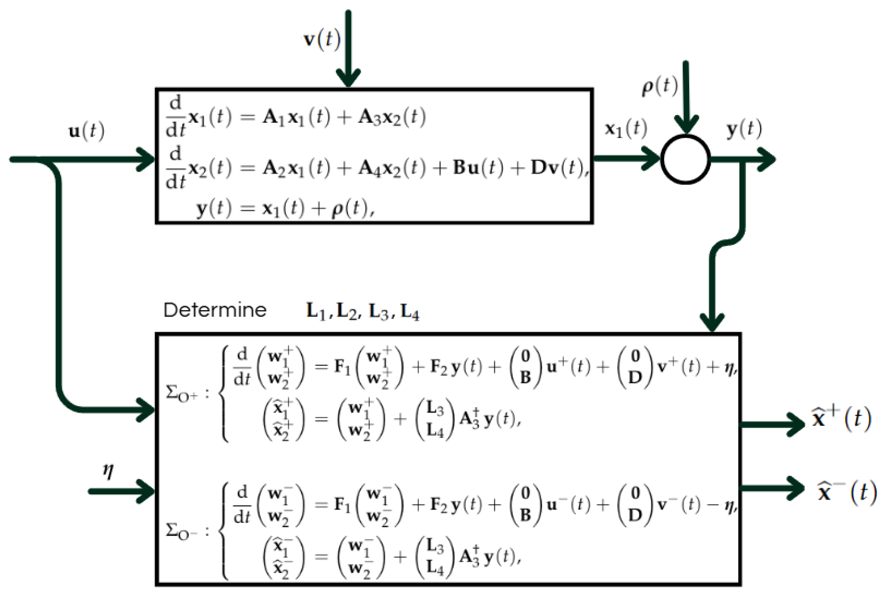
The structure of the proposed full-order interval observer is illustrated in Figure 1. This block diagram provides a graphical representation of the signal flow, including the system dynamics, the measurement noise, and the observer structure. In particular, it highlights the role of the observer gains ${\mathbf{L}}_1,{\mathbf{L}}_2,{\mathbf{L}}_3,$ and ${\mathbf{L}}_4$ in shaping the estimation error dynamics, as well as the incorporation of the term $\mathit{\eta }$. This representation complements the mathematical formulation and facilitates the interpretation of the design procedure.

To calculate the interval observer gains, we establish the following Algorithm 1.

Algorithm 1 Given that the matrices ${\mathbf{A}}_3$ and ${\mathbf{A}}_4$ satisfy Assumption 1, the estimation error matrix ${\mathbf{F}}_1$ in (13a) can be constructively assigned as follows

(1) Select a desired matrix ${\mathbf{F}}_{\mathbf{p}}\in {\mathbb{R}}^{(n_1+n_2)\times (n_1+n_2)}$ such that ${\mathbf{F}}_{\mathbf{p}}$ is Metzler and Hurwitz. (2) Partition ${\mathbf{F}}_{\mathbf{p}}$ as $${\mathbf{F}}_{\mathbf{p}}=\left(\begin{array}{cc}{\mathbf{F}}_{11}& {\mathbf{F}}_{12}\\ {\mathbf{F}}_{21}& {\mathbf{F}}_{22}\end{array}\right),$$ with compatible dimensions. (3) Compute the observer gains ${\mathbf{L}}_1,{\mathbf{L}}_2,{\mathbf{L}}_3,{\mathbf{L}}_4$ as follows: $${\mathbf{L}}_1=-{\mathbf{F}}_{11},{\mathbf{L}}_3={\mathbf{A}}_3-{\mathbf{F}}_{12},{\mathbf{L}}_2=-{\mathbf{F}}_{21},{\mathbf{L}}_4={\mathbf{A}}_4-{\mathbf{F}}_{22}.$$ (4) Construct the matrix ${\mathbf{F}}_1$ using (13a), which satisfies ${\mathbf{F}}_1={\mathbf{F}}_{\mathbf{p}}.$

Remark 2.

A possible choice to render ${\mathbf{F}}_1$ in (13a) Hurwitz and Metzler is

$$\begin{array}{c}\hfill {\mathbf{L}}_1={\ell }_1{\mathbf{I}}_{n_1},{\ell }_1>0,{\mathbf{L}}_2=0_{n_2\times n_1},{\mathbf{L}}_3={\mathbf{A}}_3,{\mathbf{L}}_4={\mathbf{A}}_4+{\ell }_4{\mathbf{I}}_{n_2},{\ell }_4>0.\end{array}$$

Please note that with this choice ${\mathbf{F}}_1=\mathrm{diag}(-{\ell }_1{\mathbf{I}}_{n_1},-{\ell }_4{\mathbf{I}}_{n_2})$, which has repeated eigenvalues $-{\ell }_1$ and $-{\ell }_4$ and non-negative off diagonal terms.

3.2. Reduced-Order Interval Observer for the Continuous-Time System

We now present a reduced-order interval observer that estimates only the unmeasured state ${\mathbf{x}}_2\left(t\right)$. We consider the observers of the following form:

$${\Sigma }_{{\mathrm{RO}}^{+}}:\left\{\begin{array}{cc}\hfill {\displaystyle \frac{\mathrm{d}}{\mathrm{d}t}}{\mathbf{w}}_2^{+}\left(t\right)& ={\mathbf{G}}_1{\mathbf{w}}_2^{+}\left(t\right)+{\mathbf{G}}_2\mathbf{y}\left(t\right)+\mathbf{B}{\mathbf{u}}^{+}\left(\mathbf{t}\right)+\mathbf{D}{\mathbf{v}}^{+}\left(\mathbf{t}\right)+\eta .\hfill \\ \hfill {\widehat{\mathbf{x}}}_2^{+}\left(t\right)& ={\mathbf{w}}_2^{+}\left(t\right)+{\mathbf{L}}_4{\mathbf{A}}_3^{†}\mathbf{y}\left(t\right).\hfill \end{array}\right.$$

(15)

$${\Sigma }_{{\mathrm{RO}}^{-}}:\left\{\begin{array}{cc}\hfill {\displaystyle \frac{\mathrm{d}}{\mathrm{d}t}}{\mathbf{w}}_2^{-}\left(t\right)& ={\mathbf{G}}_1{\mathbf{w}}_2^{-}\left(t\right)+{\mathbf{G}}_2\mathbf{y}\left(t\right)+\mathbf{B}{\mathbf{u}}^{-}\left(\mathbf{t}\right)+\mathbf{D}{\mathbf{v}}^{-}\left(\mathbf{t}\right)-\eta .\hfill \\ \hfill {\widehat{\mathbf{x}}}_2^{-}\left(t\right)& ={\mathbf{w}}_2^{-}\left(t\right)+{\mathbf{L}}_4{\mathbf{A}}_3^{†}\mathbf{y}\left(t\right).\hfill \end{array}\right.$$

(16)

where ${\mathbf{w}}_2^{\pm }\left(t\right)$ are internal observer states, and ${\widehat{\mathbf{x}}}_2^{\pm }\left(t\right)$ denote the interval estimates of ${\mathbf{x}}_2\left(t\right)$. The matrices are defined as ${\mathbf{G}}_1:={\mathbf{A}}_4-{\mathbf{L}}_4,{\mathbf{G}}_2:={\mathbf{A}}_2-{\mathbf{L}}_4{\mathbf{A}}_3^{†}{\mathbf{A}}_1+\left({\mathbf{A}}_4-{\mathbf{L}}_4\right){\mathbf{L}}_4{\mathbf{A}}_3^{†},$ and $\mathit{\eta }:=\left(\left|{\mathbf{A}}_2\right|+\left|{\mathbf{L}}_4{\mathbf{A}}_3^{†}{\mathbf{A}}_1\right|\right){\mathbf{1}}_{n_1}{r}_1+\left|{\mathbf{L}}_4{\mathbf{A}}_3^{†}\right|{\mathbf{1}}_{n_1}{r}_2$. The following theorem establishes that the pair $\left({\Sigma }_{{\mathrm{RO}}^{+}},{\Sigma }_{{\mathrm{RO}}^{-}}\right)$ form an interval observer for ${\mathbf{x}}_2\left(t\right)$.

Theorem 2.

Consider the hypotheses of Theorem 1. By choosing ${\mathbf{L}}_4$ such that the matrix ${\mathbf{A}}_4-{\mathbf{L}}_4$ is Metzler and Hurwitz, then the observers $({\Sigma }_{{\mathrm{RO}}^{+}},{\Sigma }_{{\mathrm{RO}}^{-}})$ form an interval observer for ${\mathbf{x}}_2\left(t\right)$.

Remark 3.

The Metzler property of the matrix ${\mathbf{A}}_4-{\mathbf{L}}_4$ ensures cooperativity of the observer error dynamics, which guarantees preservation of the partial order. The Hurwitz property guarantees practical stability, ensuring boundedness of the interval estimation error. By setting ${\mathbf{L}}_4={\mathbf{A}}_4+k_4\mathbf{I},k_4>0$, the observation error becomes cooperative and stable.

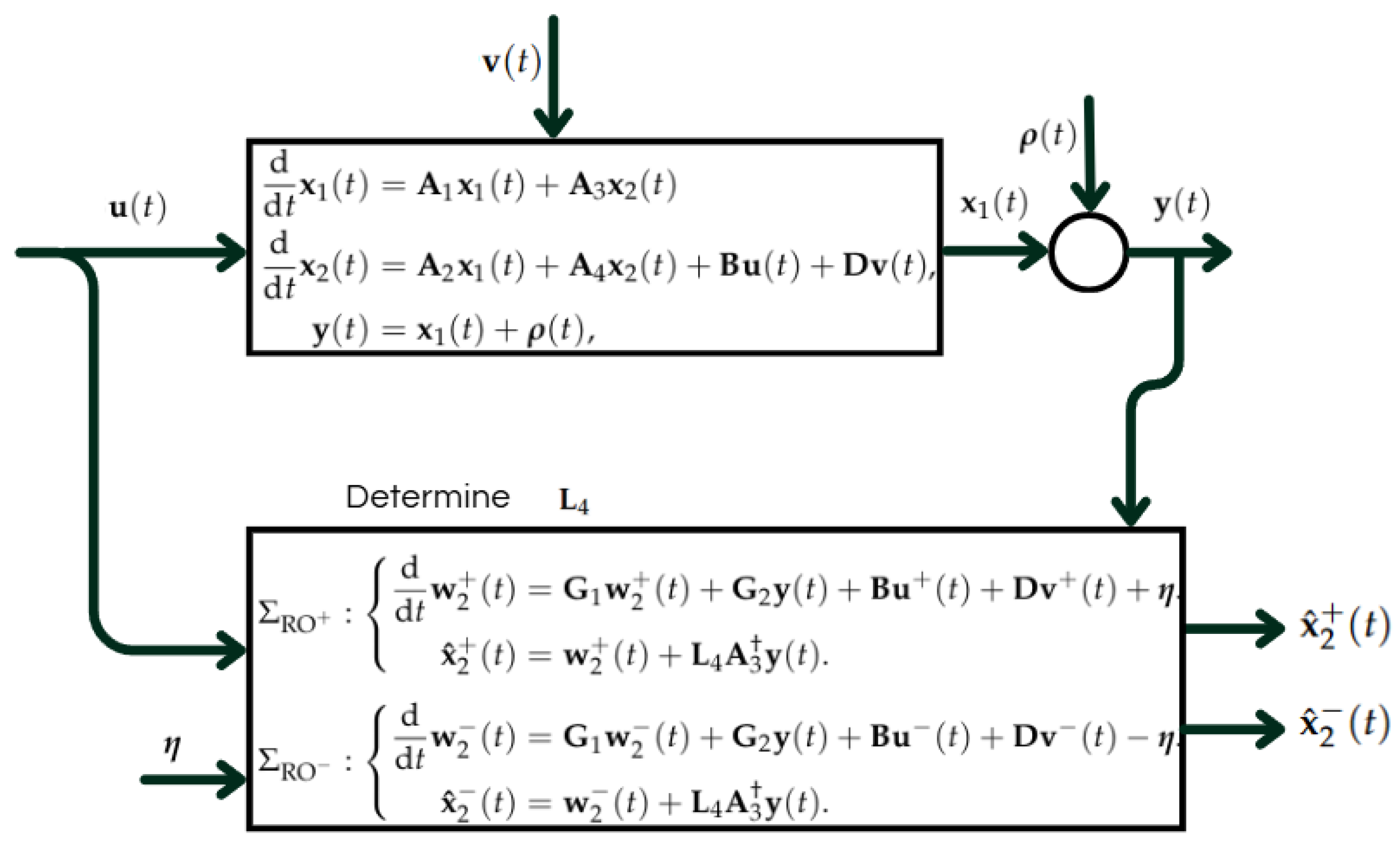
The design of the reduced-order interval observer is depicted in Figure 2. The diagram illustrates the transformation used to eliminate the dependence on the unmeasured state and emphasises the role of the gain ${\mathbf{L}}_4$ in ensuring the desired properties of the estimation error dynamics. Additionally, it shows how the bounding term $\eta$ is incorporated into the observer structure. This visual representation provides a clearer understanding of the reduced-order design and its implementation.

To complete the design of both the full-order and reduced-order interval observers, we introduce a constructive algorithm (Algorithm 2) that provides a systematic procedure for computing the observer gains such that the estimation error dynamics fulfil cooperativity and Input-to-State Stability properties.

Algorithm 2 Algorithm for computing the gains for the continuous-time interval observer for Plant (10)

Ensure: Assumptions 1, 2, and 3 in §3 are satisfied     if Full order observer in Equations (11) and (12) then           Choose: ${\mathbf{L}}_1$, ${\mathbf{L}}_2$, ${\mathbf{L}}_3$, and ${\mathbf{L}}_4$ such that ${\mathbf{F}}_1$ in (13a) is Hurwitz and Metzler           Compute: ${\mathbf{F}}_2$ and $\mathit{\eta }$ in Equations (13b) and (14), respectively     else if Reduced order observer in Equations (15) and (16) then           Choose: ${\mathbf{L}}_4$ such that ${\mathbf{G}}_1={\mathbf{A}}_4-{\mathbf{L}}_4$ is Hurwitz and Metzler           Compute: ${\mathbf{G}}_2:={\mathbf{A}}_2-{\mathbf{L}}_4{\mathbf{A}}_3^{†}{\mathbf{A}}_1+\left({\mathbf{A}}_4-{\mathbf{L}}_4\right){\mathbf{L}}_4{\mathbf{A}}_3^{†}$           Compute: $\eta :=\left(\left|{\mathbf{A}}_2\right|+\left|{\mathbf{L}}_4{\mathbf{A}}_3^{†}{\mathbf{A}}_1\right|\right){\mathbf{1}}_{n_1}{r}_1+\left|{\mathbf{L}}_4{\mathbf{A}}_3^{†}\right|{\mathbf{1}}_{n_1}{r}_2$     end if

4. Discrete-Time Interval Observers

In this section, we address the discrete-time counterparts of the full-order and reduced-order interval observer designs.

We consider the discrete-time plant, in a form analogous to (10),

$$\begin{array}{cc}\hfill {\mathbf{x}}_1[k+1]& ={\mathbf{A}}_{1\mathbf{d}}{\mathbf{x}}_1\left[k\right]+{\mathbf{A}}_{3\mathbf{d}}{\mathbf{x}}_2\left[k\right]\hfill \end{array}$$

(17a)

$$\begin{array}{cc}\hfill {\mathbf{x}}_2[k+1]& ={\mathbf{A}}_{2\mathbf{d}}{x}_1\left[k\right]+{\mathbf{A}}_{4\mathbf{d}}{x}_2\left[k\right]+{\mathbf{B}}_{\mathbf{d}}u\left[k\right]+{\mathbf{D}}_{\mathbf{d}}v\left[k\right],\hfill \end{array}$$

(17b)

$$\begin{array}{cc}\hfill \mathbf{y}\left[k\right]& ={\mathbf{x}}_1\left[k\right]+\mathit{\rho }\left[k\right],\hfill \end{array}$$

(17c)

where $({\mathbf{x}}_1\left[k\right],{\mathbf{x}}_2\left[k\right],\mathbf{y}\left[k\right],\mathbf{u}\left[k\right],\mathbf{v}\left[k\right])\in {\mathbb{R}}^{n_1}\times {\mathbb{R}}^{n_2}\times {\mathbb{R}}^{n_1}\times {\mathbb{R}}^m\times {\mathbb{R}}^q$ denote the measured state component (output up to measurement noise), the unmeasured state component, the measured output, the control input, and the unknown perturbation input, respectively. We assume that componentwise lower and upper bounds for the initial conditions, inputs, and perturbations are available as in (5), (6), and (7). Moreover, the measurement noise $\mathit{\rho }$

$${\left|\left|\mathit{\rho }\left[k\right]\right|\right|}_{\infty }\le r_1,\forall k\in \mathbb{N}.$$

(18)

4.1. Full-Order Interval Observer for the Discrete-Time System

We introduce the transformed observer coordinates ${\mathbf{w}}_i^{\pm }\left[k\right]$, $i=1,2,$ defined below, to avoid the explicit dependence on $\mathbf{y}[k+1]$ in the reconstruction of ${\mathbf{x}}_2\left[k\right]$. We propose the following discrete-time full-order interval observer, given by the expressions

$${\Sigma }_{{\mathrm{DO}}^{+}}:\left\{\begin{array}{cc}\hfill \left(\begin{array}{c}{\mathbf{w}}_1^{+}[k+1]\\ {\mathbf{w}}_2^{+}[k+1]\end{array}\right)=& {\mathbf{F}}_{1\mathbf{d}}\left(\begin{array}{c}{\mathbf{w}}_1^{+}\left[k\right]\\ {\mathbf{w}}_2^{+}\left[k\right]\end{array}\right)+{\mathbf{F}}_{2\mathbf{d}}\mathbf{y}\left[k\right]+\left(\begin{array}{c}\mathbf{0}\\ {\mathbf{B}}_{\mathbf{d}}\end{array}\right){\mathbf{u}}^{+}\left[k\right]+\left(\begin{array}{c}\mathbf{0}\\ {\mathbf{D}}_{\mathbf{d}}\end{array}\right){\mathbf{v}}^{+}\left[k\right]+{\mathit{\eta }}_d\hfill \\ \hfill \left(\begin{array}{c}{\widehat{\mathbf{x}}}_1^{+}\left[k\right]\\ {\widehat{\mathbf{x}}}_2^{+}\left[k\right]\end{array}\right)=& \left(\begin{array}{c}{\mathbf{w}}_1^{+}\left[k\right]\\ {\mathbf{w}}_2^{+}\left[k\right]\end{array}\right)+\left(\begin{array}{c}{\mathbf{L}}_{3\mathbf{d}}\\ {\mathbf{L}}_{4\mathbf{d}}\end{array}\right){\mathbf{A}}_{3\mathbf{d}}^{†}\mathbf{y}\left[k\right],\hfill \end{array}\right.$$

(19)

$${\Sigma }_{{\mathrm{DO}}^{-}}:\left\{\begin{array}{cc}\hfill \left(\begin{array}{c}{\mathbf{w}}_1^{-}[k+1]\\ {\mathbf{w}}_2^{-}[k+1]\end{array}\right)=& {\mathbf{F}}_{1\mathbf{d}}\left(\begin{array}{c}{\mathbf{w}}_1^{-}\left[k\right]\\ {\mathbf{w}}_2^{-}\left[k\right]\end{array}\right)+{\mathbf{F}}_{2\mathbf{d}}\mathbf{y}\left[k\right]+\left(\begin{array}{c}\mathbf{0}\\ {\mathbf{B}}_{\mathbf{d}}\end{array}\right){\mathbf{u}}^{-}\left[k\right]+\left(\begin{array}{c}\mathbf{0}\\ {\mathbf{D}}_{\mathbf{d}}\end{array}\right){\mathbf{v}}^{-}\left[k\right]-{\mathit{\eta }}_d\hfill \\ \hfill \left(\begin{array}{c}{\widehat{\mathbf{x}}}_1^{-}\left[k\right]\\ {\widehat{\mathbf{x}}}_2^{-}\left[k\right]\end{array}\right)=& \left(\begin{array}{c}{\mathbf{w}}_1^{-}\left[k\right]\\ {\mathbf{w}}_2^{-}\left[k\right]\end{array}\right)+\left(\begin{array}{c}{\mathbf{L}}_{3\mathbf{d}}\\ {\mathbf{L}}_{4\mathbf{d}}\end{array}\right){\mathbf{A}}_{3\mathbf{d}}^{†}\mathbf{y}\left[k\right],\hfill \end{array}\right.$$

(20)

where ${\mathbf{w}}_i^{\pm }\left[k\right],i=1,2$ represent the observer states and ${\widehat{\mathbf{x}}}_i^{\pm }\left[k\right],i=1,2$ are the upper and lower estimates. The matrices ${\mathbf{F}}_{1\mathbf{d}}$ and ${\mathbf{F}}_{2\mathbf{d}}$ are defined as

$$\begin{array}{cc}\hfill {\mathbf{F}}_{1\mathbf{d}}& :=\left(\begin{array}{cc}-{\mathbf{L}}_{1\mathbf{d}}& {\mathbf{A}}_{3\mathbf{d}}-{\mathbf{L}}_{3\mathbf{d}}\\ -{\mathbf{L}}_{2\mathbf{d}}& {\mathbf{A}}_{4\mathbf{d}}-{\mathbf{L}}_{4\mathbf{d}}\end{array}\right),\hfill \end{array}$$

(21a)

$$\begin{array}{cc}\hfill {\mathbf{F}}_{2\mathbf{d}}& :=\left(\begin{array}{c}{\mathbf{A}}_{1\mathbf{d}}-{\mathbf{L}}_{3\mathbf{d}}{\mathbf{A}}_{3\mathbf{d}}^{†}{\mathbf{A}}_{1\mathbf{d}}+({\mathbf{A}}_{3\mathbf{d}}-{\mathbf{L}}_{3\mathbf{d}}){\mathbf{L}}_{4\mathbf{d}}{\mathbf{A}}_{3\mathbf{d}}^{†}+{\mathbf{L}}_{1\mathbf{d}}({\mathbf{I}}_{n_1}-{\mathbf{L}}_{3\mathbf{d}}{\mathbf{A}}_{3\mathbf{d}}^{†})\\ {\mathbf{A}}_{2\mathbf{d}}-{\mathbf{L}}_{4\mathbf{d}}{\mathbf{A}}_{3\mathbf{d}}^{†}{\mathbf{A}}_{1\mathbf{d}}+({\mathbf{A}}_{4\mathbf{d}}-{\mathbf{L}}_{4\mathbf{d}}){\mathbf{L}}_{4\mathbf{d}}{\mathbf{A}}_{3\mathbf{d}}^{†}+{\mathbf{L}}_{2\mathbf{d}}({\mathbf{I}}_{n_1}-{\mathbf{L}}_{3\mathbf{d}}{\mathbf{A}}_{3\mathbf{d}}^{†})\end{array}\right),\hfill \end{array}$$

(21b)

where ${\mathbf{L}}_{1\mathbf{d}}\in {\mathbb{R}}^{n_1\times n_1}$, ${\mathbf{L}}_{2\mathbf{d}}\in {\mathbb{R}}^{n_2\times n_1}$, ${\mathbf{L}}_{3\mathbf{d}}\in {\mathbb{R}}^{n_1\times n_2}$, ${\mathbf{L}}_{4\mathbf{d}}\in {\mathbb{R}}^{n_2\times n_2}$ are the observer gains. We assume that ${\mathbf{A}}_{3\mathbf{d}}$ admits a left inverse ${\mathbf{A}}_{3\mathbf{d}}^{†}\in {\mathbb{R}}^{n_2\times n_1}$ satisfying ${\mathbf{A}}_{3\mathbf{d}}^{†}{\mathbf{A}}_{3\mathbf{d}}={\mathbf{I}}_{n_2}$. The vector ${\mathit{\eta }}_{\mathbf{d}}\in {\mathbb{R}}^{n_1+n_2}$ is selected to upper-bound the worst-case contribution of bounded measurement noise in the transformed dynamics, and is defined as

$$\begin{array}{c}\hfill {\mathit{\eta }}_d:=\left(\begin{array}{c}\hfill {\mathbf{I}}_{n_1}+\left|{\mathbf{A}}_{1\mathbf{d}}\right|+\left|{\mathbf{L}}_{\mathbf{3}\mathbf{d}}{\mathbf{A}}_{\mathbf{3}\mathbf{d}}^{†}{\mathbf{A}}_{\mathbf{1}\mathbf{d}}\right|+\left|{\mathbf{L}}_{\mathbf{3}\mathbf{d}}{\mathbf{A}}_{\mathbf{3}\mathbf{d}}^{†}\right|\\ \hfill \left|{\mathbf{A}}_{2\mathbf{d}}\right|+\left|{\mathbf{L}}_{\mathbf{4}\mathbf{d}}{\mathbf{A}}_{\mathbf{3}\mathbf{d}}^{†}{\mathbf{A}}_{\mathbf{1}\mathbf{d}}\right|+\left|{\mathbf{L}}_{\mathbf{4}\mathbf{d}}{\mathbf{A}}_{\mathbf{3}\mathbf{d}}^{†}\right|\end{array}\right)r_1{\mathbf{1}}_n.\end{array}$$

(22)

Theorem 3.

Consider Assumptions 1 and 2, and let $\mathit{\rho }\left[k\right]$ satisfy (18). Additionally, let the gains be chosen such that ${\mathbf{F}}_{1\mathbf{d}}⪰\mathbf{0}$ and $\varrho \left({\mathbf{F}}_{1\mathbf{d}}\right)<1$. Then, the observer pair (19) and (20) constitutes an interval observer for discrete-time system (17), such that

$${\widehat{\mathbf{x}}}^{+}\left[k\right]⪰\mathbf{x}\left[k\right]⪰{\widehat{\mathbf{x}}}^{-}\left[k\right],\forall k\in \mathbb{N}.$$

Remark 4.

The choice ${\mathbf{L}}_{1\mathbf{d}}={\ell }_{1\mathbf{d}}{\mathbf{I}}_{n_1},{\ell }_{1\mathbf{d}}\in \left(-1,0\right),{\mathbf{L}}_{2\mathbf{d}}=0_{n_2\times n_1},{\mathbf{L}}_{3\mathbf{d}}={\mathbf{A}}_{3\mathbf{d}},{\mathbf{L}}_{4\mathbf{d}}={\mathbf{A}}_4+{\ell }_{4\mathbf{d}}{\mathbf{I}}_{n_2},{\ell }_{4\mathbf{d}}\in \left(-1,0\right)$ renders ${\mathbf{F}}_{1\mathbf{d}}$ in (21a) both non-negative and Schur-stable.

Please note that with this choice ${\mathbf{F}}_{1\mathrm{d}}=\mathrm{diag}(-{\ell }_1{\mathbf{I}}_{n_1},-{\ell }_4{\mathbf{I}}_{n_2})$.

4.2. Reduced-Order Interval Observer or the Discrete-Time System

As in the continuous-time case, a reduced-order interval observer can be constructed in order to estimate only the unmeasured state ${\mathbf{x}}_2\left[k\right]$. To this end, consider

$${\Sigma }_{{\mathrm{DRO}}^{+}}:\left\{\begin{array}{cc}\hfill {\mathbf{w}}_2^{+}[k+1]& ={\mathbf{G}}_{1\mathrm{d}}{\mathbf{w}}_2^{+}\left[k\right]+{\mathbf{G}}_{2\mathrm{d}}\mathbf{y}\left[k\right]+{\mathbf{B}}_{\mathrm{d}}{\mathbf{u}}^{+}\left[k\right]+{\mathbf{D}}_{\mathrm{d}}{\mathbf{v}}^{+}\left[k\right]+{\mathit{\eta }}_{\mathrm{d}}.\hfill \\ \hfill {\widehat{\mathbf{x}}}_2^{+}\left[k\right]& ={\mathbf{w}}_2^{+}\left[k\right]+{\mathbf{L}}_{4\mathrm{d}}{\mathbf{A}}_{3\mathrm{d}}^{†}\mathbf{y}\left[k\right].\hfill \end{array}\right.$$

(23)

$${\Sigma }_{{\mathrm{DRO}}^{-}}:\left\{\begin{array}{cc}\hfill {\mathbf{w}}_2^{-}[k+1]& ={\mathbf{G}}_{1\mathrm{d}}{\mathbf{w}}_2^{-}\left[k\right]+{\mathbf{G}}_{2\mathrm{d}}\mathbf{y}\left[k\right]+{\mathbf{B}}_{\mathrm{d}}{\mathbf{u}}^{-}\left[k\right]+{\mathbf{D}}_{\mathrm{d}}{\mathbf{v}}^{-}\left[k\right]-{\mathsf{\eta }}_{\mathrm{d}}.\hfill \\ \hfill {\widehat{\mathbf{x}}}_2^{-}\left[k\right]& ={\mathbf{w}}_2^{-}\left[k\right]+{\mathbf{L}}_{4\mathrm{d}}{\mathbf{A}}_{3\mathrm{d}}^{†}\mathbf{y}\left[k\right],\hfill \end{array}\right.$$

(24)

where ${\mathbf{w}}_2^{\pm }\left[k\right]$ are the internal observer states, and ${\widehat{\mathbf{x}}}_2^{\pm }\left[k\right]$ denote the interval estimates of ${\mathbf{x}}_2\left[k\right]$, with the matrices ${\mathbf{G}}_{1\mathrm{d}}:={\mathbf{A}}_{4\mathrm{d}}-{\mathbf{L}}_{4\mathrm{d}},{\mathbf{G}}_{2\mathrm{d}}:={\mathbf{A}}_{2\mathrm{d}}-{\mathbf{L}}_{4\mathrm{d}}{\mathbf{A}}_{3\mathrm{d}}^{†}{\mathbf{A}}_{1\mathrm{d}}+\left({\mathbf{A}}_{4\mathrm{d}}-{\mathbf{L}}_{4\mathrm{d}}\right){\mathbf{L}}_{4\mathrm{d}}{\mathbf{A}}_{3\mathrm{d}}^{†},$ and

$$\begin{array}{cc}\hfill {\mathit{\eta }}_{\mathrm{d}}& :=\left(\left|{\mathbf{A}}_{2\mathrm{d}}\right|+\left|{\mathbf{L}}_{\mathbf{4}\mathrm{d}}{\mathbf{A}}_{\mathbf{3}\mathrm{d}}^{†}{\mathbf{A}}_{\mathbf{1}\mathrm{d}}\right|+\left|{\mathbf{L}}_{\mathbf{4}\mathrm{d}}{\mathbf{A}}_{\mathbf{3}\mathrm{d}}^{†}\right|\right){\mathbf{1}}_{n_1}{r}_1.\hfill \end{array}$$

(25)

The following theorem states the design conditions of the reduced-order interval observers $\left({\Sigma }_{{\mathrm{DRO}}^{+}},{\Sigma }_{{\mathrm{DRO}}^{-}}\right)$ for the discrete-time plant (17).

A preliminary version of this result was presented in [40], where no measurement noise was considered, $n_1=n_2$, and ${\mathbf{A}}_{\mathbf{1}}=\mathbf{0}$ and ${\mathbf{A}}_{\mathbf{3}}=\mathbf{I}$.

Theorem 4.

Consider the hypothesis of Theorem 3. Let ${\mathbf{L}}_{4d}$ be chosen such that the matrix ${\mathbf{G}}_{1d}$ is non-negative and Schur-stable. Then, the observers (23) and (24) are an interval observer for ${\mathbf{x}}_2\left[k\right]$ in (17).

Now, Algorithm 3 shows a design procedure for the discrete-time observers. The key difference w.r.t. the continuous-time one is that the desired matrices ${\mathbf{F}}_{1\mathrm{d}}$ and ${\mathbf{G}}_{1\mathrm{d}}$ are Schur-stable and non-negative. To define matrices with those properties, one may choose diagonal matrices (as in Remarks 4) or triangular matrices, ensuring that the diagonal entries, i.e., the eigenvalues of the matrices, are smaller than one. To set a more general matrix ${\mathbf{F}}_{1\mathrm{d}}$, one may use Algorithm 1, considering that the target matrix is non-negative and Schur-stable.

Algorithm 3 Algorithm for computing the gains for the discrete-time interval observer for Plant (17)

Ensure: Assumptions 1 and 2 in Section 3, along with a bound for the measurement noise $\mathit{\rho }\left[k\right]$ in Equation (18) are satisfied     if Full order observer in Equations (19) and (20) then         Choose: ${\mathbf{L}}_{1\mathrm{d}}$, ${\mathbf{L}}_{2\mathrm{d}}$, ${\mathbf{L}}_{3\mathrm{d}}$, and ${\mathbf{L}}_{4\mathrm{d}}$ such that ${\mathbf{F}}_{1\mathrm{d}}$ in (21a) is Schur-stable and non-negative         Compute: ${\mathbf{F}}_{2\mathrm{d}}$ and ${\mathit{\eta }}_d$ in Equaitons (21b) and (22), respectively     else if Reduced order observer in Equations (23) and (24) then         Choose: ${\mathbf{L}}_{4\mathrm{d}}$ such that ${\mathbf{G}}_{1\mathrm{d}}={\mathbf{A}}_{4\mathrm{d}}-{\mathbf{L}}_{4\mathrm{d}}$ is Schur-stable and non-negative         Compute: ${\mathbf{G}}_{2\mathrm{d}}:={\mathbf{A}}_{2\mathrm{d}}-{\mathbf{L}}_{4\mathrm{d}}{\mathbf{A}}_{3\mathrm{d}}^{†}{\mathbf{A}}_{1\mathrm{d}}+\left({\mathbf{A}}_{4\mathrm{d}}-{\mathbf{L}}_{4\mathrm{d}}\right){\mathbf{L}}_{4\mathrm{d}}{\mathbf{A}}_{3\mathrm{d}}^{†}$         Compute: ${\mathit{\eta }}_d:=\left(\left|{\mathbf{A}}_{2d}\right|+\left|{\mathbf{L}}_{\mathbf{4}\mathbf{d}}{\mathbf{A}}_{\mathbf{3}\mathbf{d}}^{†}{\mathbf{A}}_{\mathbf{1}\mathbf{d}}\right|+\left|{\mathbf{L}}_{\mathbf{4}\mathbf{d}}{\mathbf{A}}_{\mathbf{3}\mathbf{d}}^{†}\right|\right){\mathbf{1}}_{n_1}{r}_1$     end if

5. Numerical Examples

In this section, we present three examples related to the design of interval observers for linear systems. The first example considers the design for the continuous-time interval observer, while the second includes the design for the discrete-time case. In both cases, we design a full and a reduced observer. At a later stage, we consider an interval observer for a mechanical system in continuous and discrete-time.

5.1. Continuos-Time Observer

Let us consider the following plant, which is in the form of Equation (10).

$$\begin{array}{cc}\hfill {\displaystyle \frac{\mathrm{d}}{\mathrm{d}t}}{\mathbf{x}}_1\left(t\right)& =\left(\begin{array}{cc}-1.3623& -1.7593\\ -1.0423& -1.3239\end{array}\right){\mathbf{x}}_1\left(t\right)+\left(\begin{array}{cc}0.2548& 0.6678\\ 0.2240& 0.8444\end{array}\right){\mathbf{x}}_2\left(t\right)\hfill \end{array}$$

(26a)

$$\begin{array}{cc}\hfill {\displaystyle \frac{\mathrm{d}}{\mathrm{d}t}}{\mathbf{x}}_2\left(t\right)& =\left(\begin{array}{cc}0.2891& 0.6951\\ 0.6718& 0.0680\end{array}\right){\mathbf{x}}_{\mathbf{1}}\left(\mathbf{t}\right)+\left(\begin{array}{cc}-4.6555& -4.3247\\ -4.2195& -4.9933\end{array}\right){\mathbf{x}}_{\mathbf{2}}\left(\mathbf{t}\right)+\left(\begin{array}{c}0.6022\\ 0.3868\end{array}\right)\mathbf{u}\left(\mathbf{t}\right)\hfill \\ & +\left(\begin{array}{c}0.9160\\ 0.0012\end{array}\right)\mathbf{v}\left(\mathbf{t}\right),\hfill \end{array}$$

(26b)

$$\begin{array}{cc}\hfill \mathbf{y}\left(t\right)& ={\mathbf{x}}_1\left(t\right).\hfill \end{array}$$

(26c)

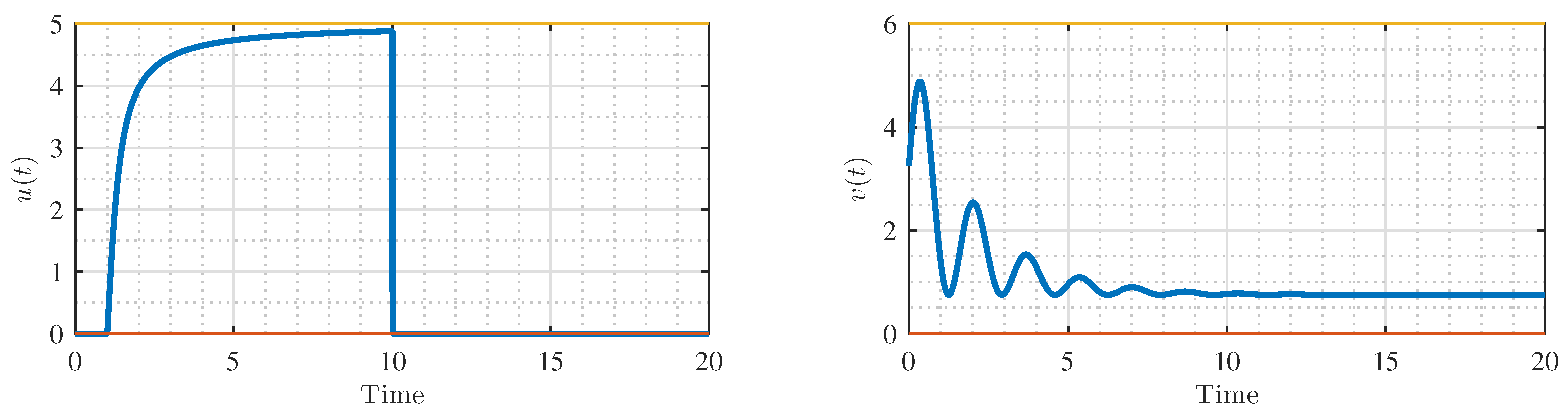
Note that the number of measured states, $n_1$, is equal to that of the unmeasured ones, $n_2$. Thus, Assumption 1 is fulfilled. In addition, the input, perturbation, and output matrices above are non-negative. The control input and the perturbation are time-varying signals but bounded within intervals, $5>u\left(t\right)>0, 6>v\left(t\right)>0.$

Figure 3 shows the applied inputs to the system in (26). In the scalar case, the control input $u\left(t\right)$ satisfies the inequality ${\mathbf{u}}^{+}\left(t\right)⪰\mathbf{u}\left(t\right)⪰{\mathbf{u}}^{-}\left(t\right),\forall t\ge 0$, where ${\mathbf{u}}^{+}\left(t\right)=5$ and ${\mathbf{u}}^{-}\left(t\right)=0$ represent the upper and lower bounds of $\mathbf{u}\left(t\right)$, respectively. Similarly, the perturbation $v\left(t\right)$ is bounded according to ${\mathbf{v}}^{+}\left(t\right)⪰\mathbf{v}\left(t\right)⪰{\mathbf{v}}^{-}\left(t\right)$, with ${\mathbf{v}}^{+}\left(t\right)=6$ and ${\mathbf{v}}^{-}\left(t\right)=0$.

In this example, two simulation scenarios will be considered to illustrate the behaviour of the proposed interval observer designs for the system (26) in the presence of bounded perturbations $\mathbf{v}\left(t\right)$ and measurement noise $\mathit{\rho }\left(t\right)$:

i.

A full-order interval observer is designed to provide upper and lower estimates for all the system states, $\mathbf{x}\left(t\right)={\left[{\mathbf{x}}_1\left(t\right){\mathbf{x}}_2\left(t\right)\right]}^{\top }$, relying on the outputs of the first subsystem.

ii.

A reduced-order interval observer is developed, whose dimension is lower than that of the plant, to generate the interval estimates only of the unmeasured states ${\mathbf{x}}_2\left(t\right)$ from available measurements.

5.1.1. Full-Order Interval Observer Design

In this scenario, we design the full-order interval observer, by ensuring that the conditions of Theorem 1 are fulfilled.

By taking into account Remark 2, let the interval observer’s gains be

$$\begin{array}{c}\hfill {\mathbf{L}}_1=5{\mathbf{I}}_2=\left(\begin{array}{cc}5& 0\\ 0& 5\end{array}\right),{\mathbf{L}}_2={\mathbf{0}}_{2x2},{\mathbf{L}}_3={\mathbf{A}}_3=\left(\begin{array}{cc}0.2548& 0.6678\\ 0.2240& 0.8444\end{array}\right),{\mathbf{L}}_4=\left(\begin{array}{cc}10.3445& -4.3247\\ -4.2195& 10.0067\end{array}\right)\end{array}$$

$$\begin{array}{c}\hfill \mathrm{thus},{\mathbf{F}}_{\mathbf{1}}=\mathrm{diag}\{-5,-5,-15,-15\},{\mathbf{F}}_{\mathbf{2}}=1\times {10}^3\left(\begin{array}{cc}0& 0\\ 0& 0\\ -2.1469& 1.9332\\ 1.2943& -1.2761\end{array}\right).\end{array}$$

The initial conditions for the full-order interval observer were chosen as ${\widehat{\mathbf{x}}}_1^{+}\left(0\right)={\left[11\right]}^{\top }$, ${\widehat{\mathbf{x}}}_2^{+}\left(0\right)={\left[11\right]}^{\top }$, ${\widehat{\mathbf{x}}}_1^{-}\left(0\right)={\left[00\right]}^{\top }$, and ${\widehat{\mathbf{x}}}_2^{-}\left(0\right)={\left[00\right]}^{\top }$, while the initial states of the plant were ${\mathbf{x}}_1\left(t\right)={\left[0.50\right]}^{\top }$ and ${\mathbf{x}}_2\left(t\right)={\left[00.1\right]}^{\top }$, such that the interval inequality ${\widehat{\mathbf{x}}}^{+}\left(0\right)⪰\mathbf{x}\left(0\right)⪰{\widehat{\mathbf{x}}}^{-}\left(0\right),$ is satisfied, with $\mathbf{x}\left(0\right)={\left[{\mathbf{x}}_1\left(0\right){\mathbf{x}}_2\left(0\right)\right]}^{\top }$ and ${\widehat{\mathbf{x}}}^i\left(0\right)={\left[{\widehat{\mathbf{x}}}_1^i\left(0\right){\widehat{\mathbf{x}}}_2^i\left(0\right)\right]}^{\top }$, with $i=+,-$.

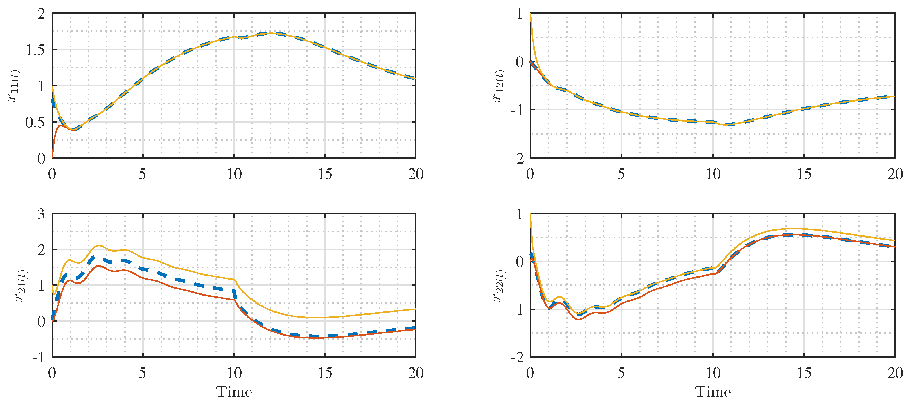
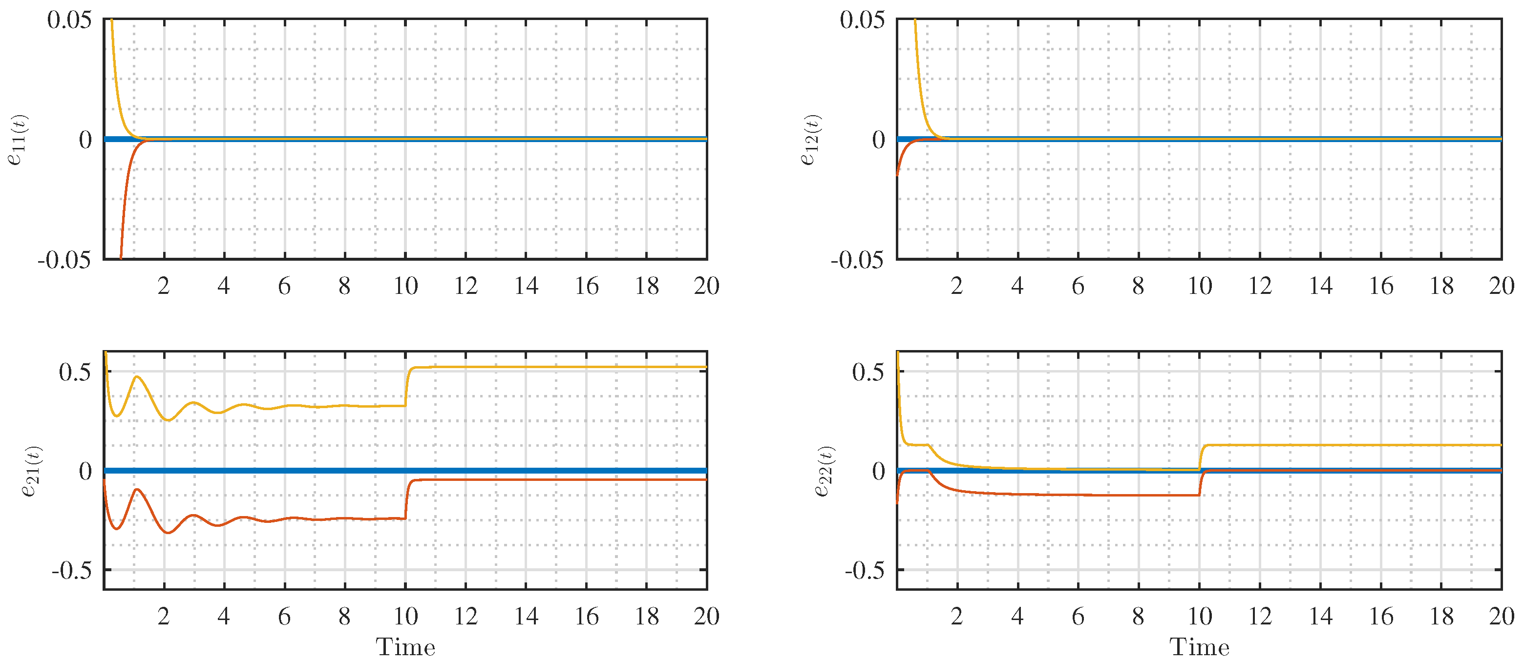
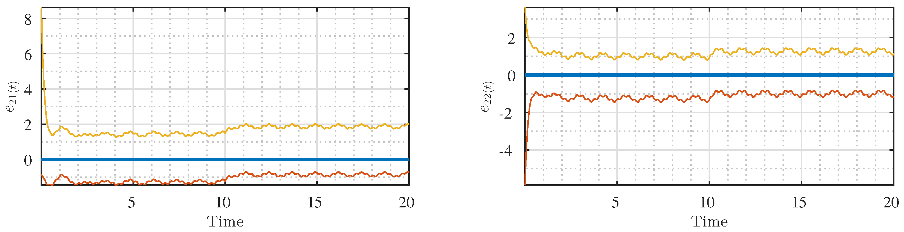
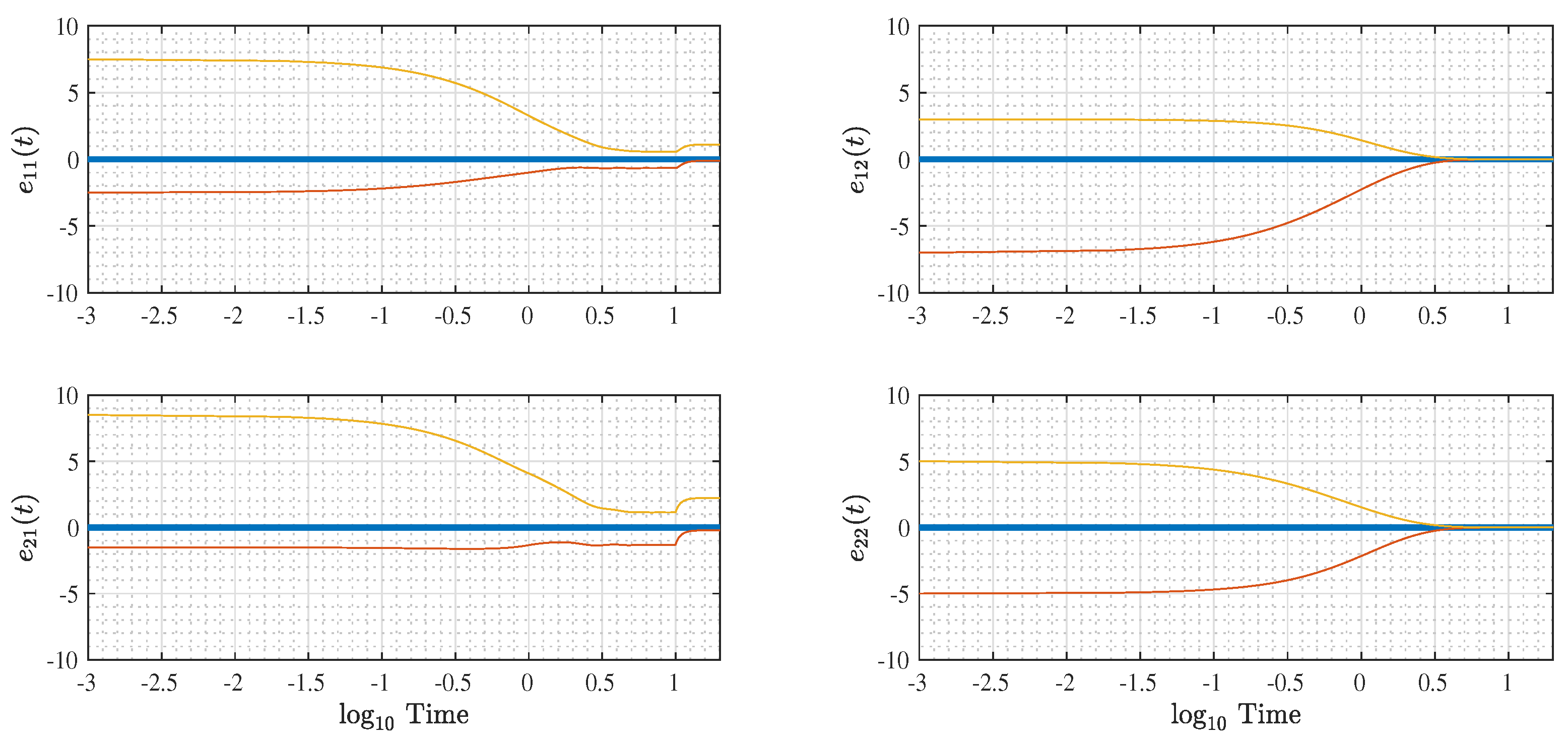
Figure 4 illustrates the dynamic behaviour of the full-order interval observer $({\Sigma }_{{\mathrm{O}}^{+}},{\Sigma }_{{\mathrm{O}}^{-}})$ applied to the system (26), where the upper and lower estimations fulfill the partial ordering and practical convergence properties with respect to the trajectories of the state, satisfying the expression ${\widehat{\mathbf{x}}}^{+}\left(t\right)⪰\mathbf{x}\left(t\right)⪰{\widehat{\mathbf{x}}}^{-}\left(t\right),\forall t\ge 0,$ from the partial ordering assumed for the initial conditions and input signals. Moreover, the estimation errors are depicted in Figure 5 under above conditions ${\mathbf{e}}^{+}\left(t\right)={\widehat{\mathbf{x}}}^{+}\left(t\right)-\mathbf{x}\left(t\right)$ and ${\mathbf{e}}^{-}\left(t\right)=\mathbf{x}\left(t\right)-{\widehat{\mathbf{x}}}^{-}\left(t\right)$. Note that the estimation errors ${\mathbf{e}}_{2j}\left(t\right)$, with $j=1,2$, are expected to preserve the partial ordering and converge asymptotically to an ultimate bound in the presence of the control input and the perturbation.

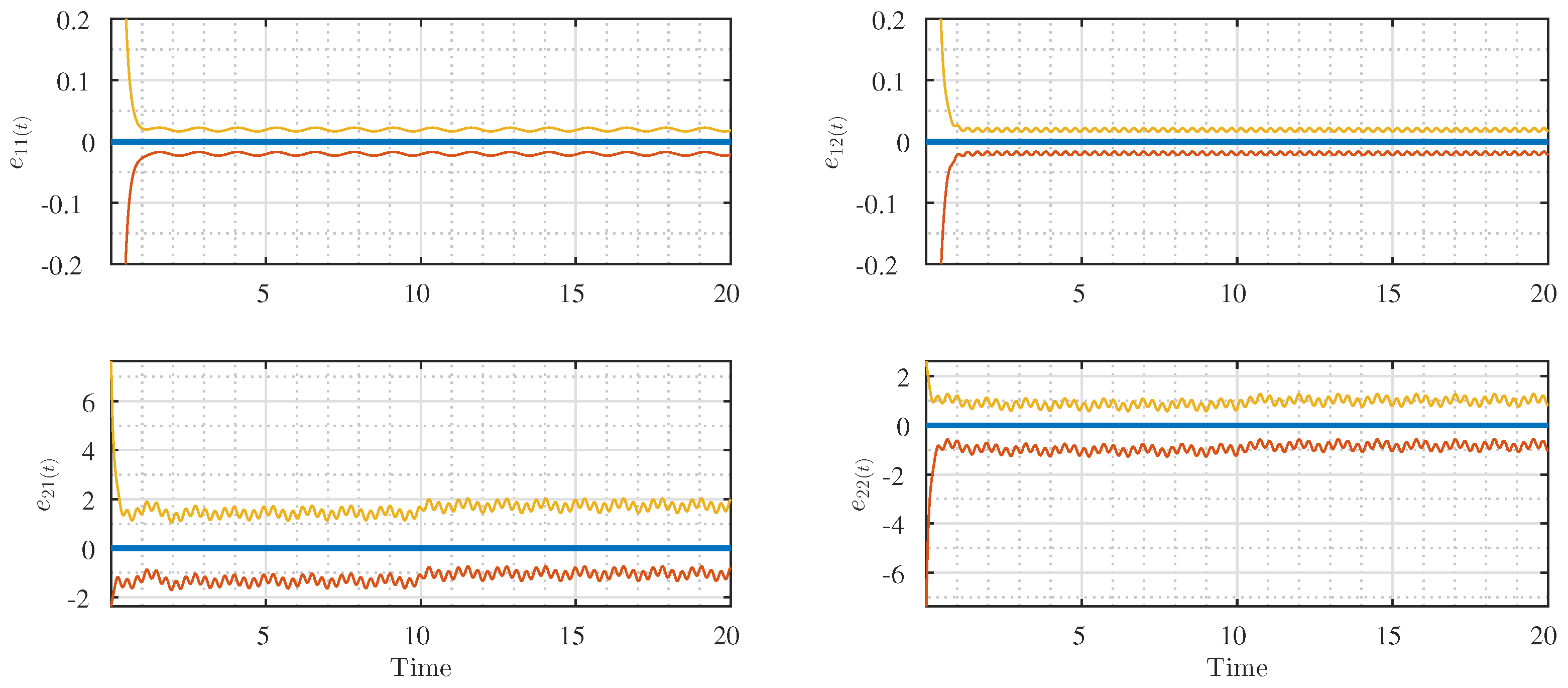
In this scenario, the trajectories of the interval estimation errors, under levels of measurement noise and external perturbations, are depicted in Figure 6. The measurement noise used were $\mathit{\rho }\left(t\right)=3\times {10}^{-3}{\left(\begin{array}{cc}sin\left(5t\right)& sin\left(20t\right)\end{array}\right)}^{\top }$, and the upper bounds for the noise and its derivative were set as $r_1=3\times {10}^{-3}$ and $r_2=60\times {10}^{-3}$, respectively. Using these simulation conditions, it is easy to verify that the inequality ${\widehat{\mathbf{x}}}^{+}\left(t\right)⪰\mathbf{x}\left(t\right)⪰{\widehat{\mathbf{x}}}^{-}\left(t\right),\forall t\ge 0,$ is satisfied, which demonstrates the robustness and monotonicity (cooperativity) properties of the proposed interval observer based on the design of Theorem 1.

5.1.2. Reduced-Order Interval Observer Design

Analogously, in this scenario, we design the reduced-order interval observer for Plant (26), now ensuring the conditions of Theorem 2. Thus, we choose the design matrices as

$$\begin{array}{c}\hfill {\mathbf{L}}_4={\mathbf{A}}_{\mathbf{4}}+15\mathbf{I}=\left(\begin{array}{c}10.3445-4.3247\\ -4.219510.0067\end{array}\right),{\mathbf{G}}_1=\left(\begin{array}{c}-150\\ 0-15\end{array}\right),{\mathbf{G}}_2=1\times {10}^3\left(\begin{array}{c}-2.14691.9332\\ 1.2943-1.2761\end{array}\right).\end{array}$$

The initial conditions for the reduced-order interval observer were selected as ${\widehat{\mathbf{x}}}_2^{+}{\left(0\right)}^{=}{\left[11\right]}^{\top }$ and ${\widehat{\mathbf{x}}}_2^{-}{\left(0\right)}^{=}{\left[00\right]}^{\top }$, while the initial state of the plant was ${\mathbf{x}}_2\left(t\right)={\left[0.50.5\right]}^{\top }$, such that the interval inequality ${\widehat{\mathbf{x}}}_2^{+}\left(0\right)⪰{\mathbf{x}}_2\left(0\right)⪰{\widehat{\mathbf{x}}}_2^{-}\left(0\right),$ is fulfilled.

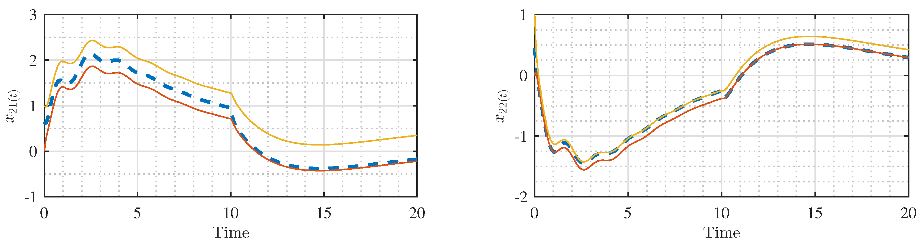
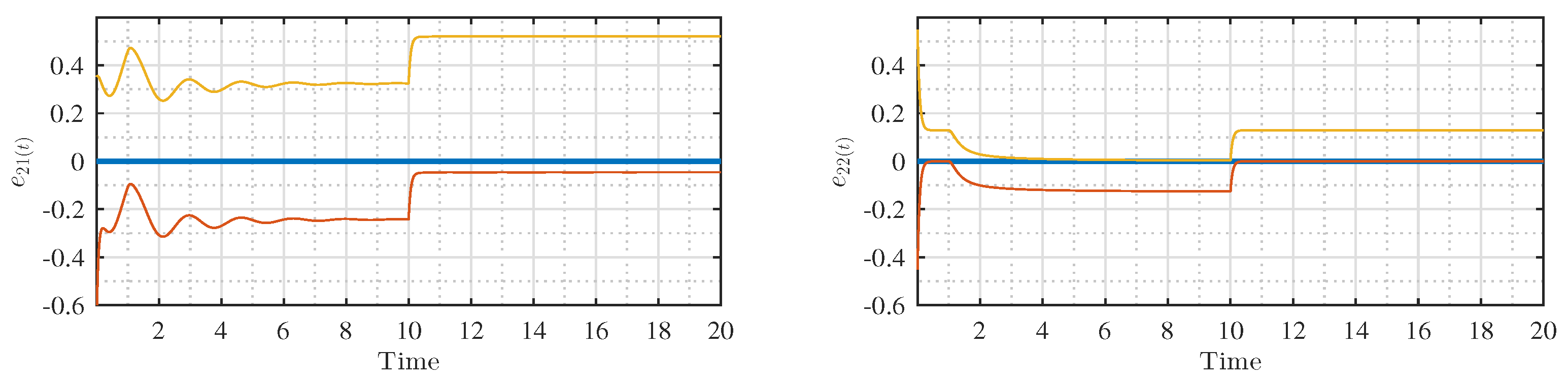
Under the same simulation conditions for the inputs presented in Figure 3, Figure 7 and Figure 8 show the responses of the interval estimated states and estimation errors for this scenario. Furthermore, Figure 9 presents the estimation error with measurement noise, considering the same levels as in the full-order interval observer case. It is clear to see that the reduced-order interval observer preserves the partial ordering and practical convergence properties with respect to the trajectories of state ${\mathbf{x}}_2$, which guarantees the interval relation ${\widehat{\mathbf{x}}}_2^{+}\left(t\right)⪰{\mathbf{x}}_2\left(t\right)⪰{\widehat{\mathbf{x}}}_2^{-}\left(t\right),\forall t\ge 0$.

5.2. Discrete-Time Observers

In this subsection, we present a numerical example to illustrate the performance of the proposed interval observers in the discrete-time setting, following the scenarios previously presented in the continuous-time case.

We consider the following discrete-time plant, with a sampling step of $\tau =0.3$,

$$\begin{array}{cc}\hfill {\mathbf{x}}_1[k+1]& =\left(\begin{array}{cc}0.1272& 0.5483\\ 0.0464& 0.4240\end{array}\right){\mathbf{x}}_1\left[k\right]+\left(\begin{array}{cc}0.0988& 0.0258\\ 0.0170& 0.0397\end{array}\right){\mathbf{x}}_2\left[k\right]\hfill \end{array}$$

(27a)

$$\begin{array}{cc}\hfill {\mathbf{x}}_2[k+1]& =\left(\begin{array}{cc}0.0558& 0.0166\\ 0.0313& 0.0622\end{array}\right){\mathbf{x}}_{\mathbf{1}}\left[k\right]+\left(\begin{array}{cc}0.0444& 0.2414\\ 0.4105& 0.5897\end{array}\right){\mathbf{x}}_{\mathbf{2}}\left[k\right]+\left(\begin{array}{c}0.4022\\ 0.6207\end{array}\right)\mathbf{u}\left[k\right]\hfill \\ & +\left(\begin{array}{c}0.1544\\ 0.3813\end{array}\right)\mathbf{v}\left[k\right],\hfill \end{array}$$

(27b)

$$\begin{array}{cc}\hfill \mathbf{y}\left[k\right]& ={\mathbf{x}}_1\left[k\right].\hfill \end{array}$$

(27c)

Similarly to the continuous case, we assume that the upper and lower bounds are available for the initial conditions, inputs, and perturbations.

5.2.1. Discrete-Time Full-Order Interval Observer

In this part, a discrete-time full-order interval observer is designed according to Theorem 3.

By considering Remark 4, the observer gains are chosen as

$$\begin{array}{cc}\hfill {\mathbf{L}}_{1\mathrm{d}}& =\left(\begin{array}{cc}-0.2& 0\\ 0& -0.2\end{array}\right),{\mathbf{L}}_{2\mathrm{d}}={\mathbf{0}}_{2x2},{\mathbf{L}}_{3\mathrm{d}}={\mathbf{A}}_{3\mathrm{d}}=\left(\begin{array}{cc}0.0988& 0.0258\\ 0.0170& 0.0397\end{array}\right),\hfill \\ \hfill {\mathbf{L}}_{4\mathrm{d}}& ={\mathbf{A}}_{\mathbf{4}\mathrm{d}}-0.2{\mathbf{I}}_2=\left(\begin{array}{cc}-0.1556& 0.2414\\ 0.4105& 0.3897\end{array}\right).\hfill \end{array}$$

With this choice, the matrices of the observer dynamics are

$$\begin{array}{c}\hfill {\mathbf{F}}_{1\mathrm{d}}=\left(\begin{array}{cccc}0.2& 0& 0& 0\\ 0& 0.2& 0& 0\\ 0& 0& 0.2& 0\\ 0& 0& 0& 0.2\end{array}\right),{\mathbf{F}}_{2\mathrm{d}}=\left(\begin{array}{cc}0& 0\\ 0& 0\\ -0.5309& -0.1560\\ -0.1392& -3.2539\end{array}\right),\end{array}$$

which endows the state matrix of the observation error, ${\mathbf{F}}_1$, with repeated eigenvalues in 0.2.

The initial conditions for the full-order (discrete time) interval observer were chosen as ${\widehat{\mathbf{x}}}_1^{+}\left(0\right)={\left[55\right]}^{\top }$, ${\widehat{\mathbf{x}}}_2^{+}\left(0\right)={\left[55\right]}^{\top }$, ${\widehat{\mathbf{x}}}_1^{-}\left(0\right)={\left[00\right]}^{\top }$, and ${\widehat{\mathbf{x}}}_2^{-}\left(0\right)={\left[00\right]}^{\top }$, while the initial states of the plant were ${\mathbf{x}}_1\left(t\right)={\left[1.23.5\right]}^{\top }$ and ${\mathbf{x}}_2\left(t\right)={\left[0.92.5\right]}^{\top }$, such that the interval inequality ${\widehat{\mathbf{x}}}^{+}\left(0\right)⪰\mathbf{x}\left(0\right)⪰{\widehat{\mathbf{x}}}^{-}\left(0\right),$ is satisfied, with $\mathbf{x}\left(0\right)={\left[{\mathbf{x}}_1\left(0\right){\mathbf{x}}_2\left(0\right)\right]}^{\top }$ and ${\widehat{\mathbf{x}}}^i\left(0\right)={\left[{\widehat{\mathbf{x}}}_1^i\left(0\right){\widehat{\mathbf{x}}}_2^i\left(0\right)\right]}^{\top }$, with $i=+,-$.

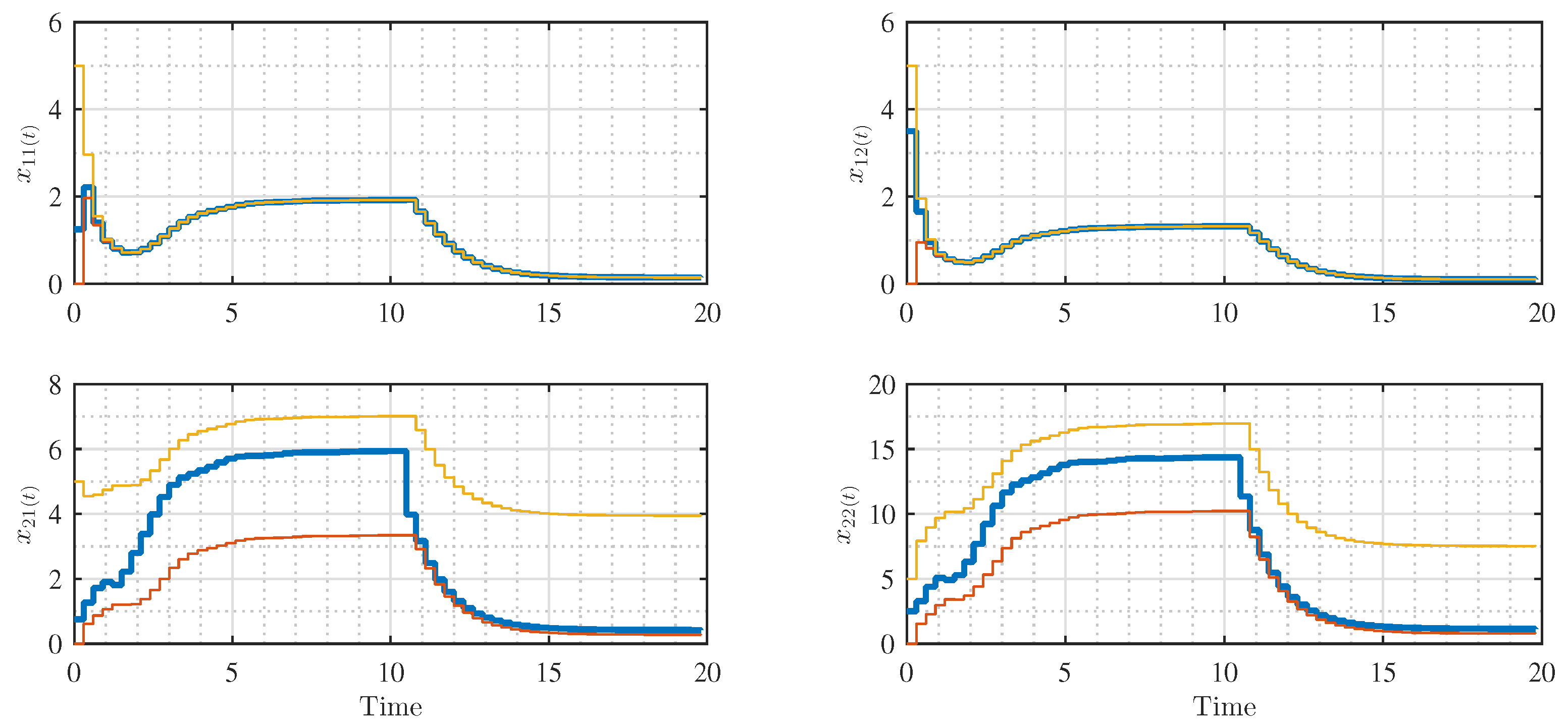
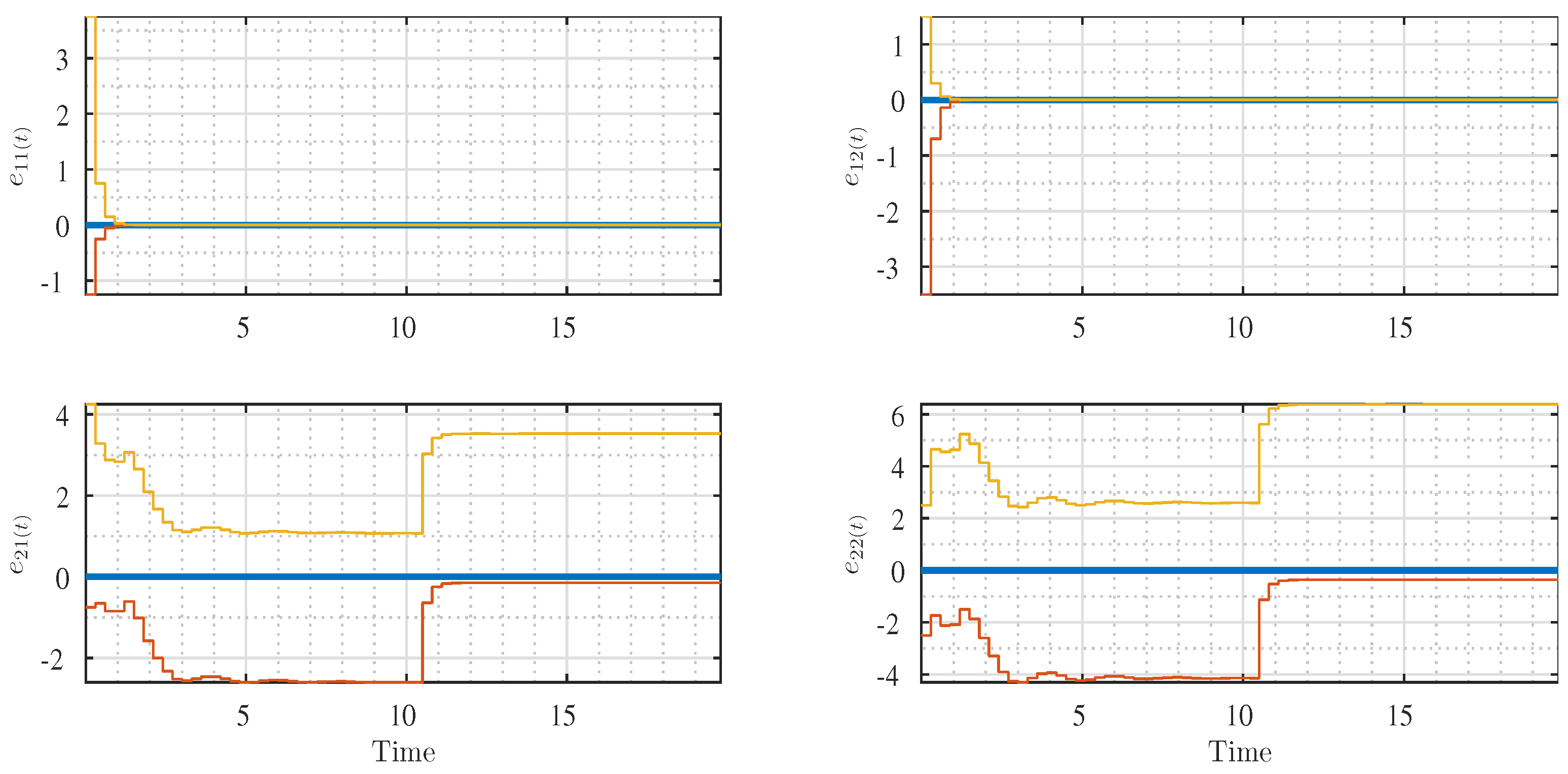
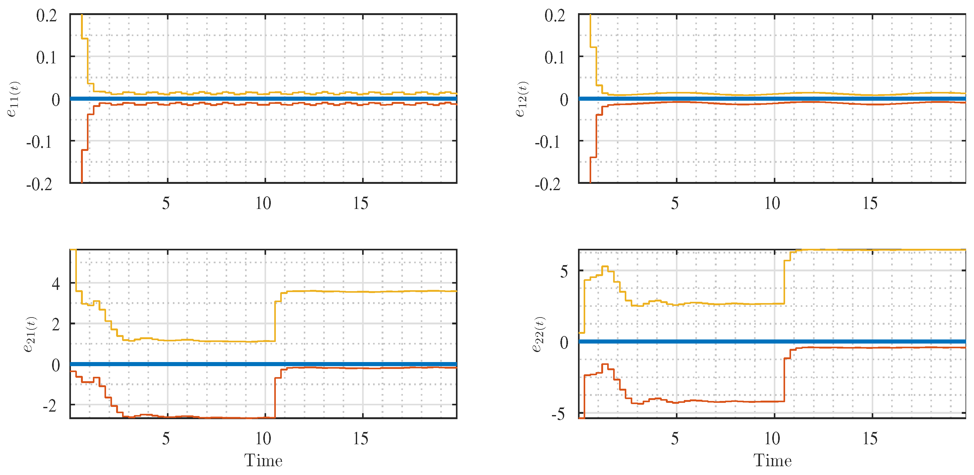
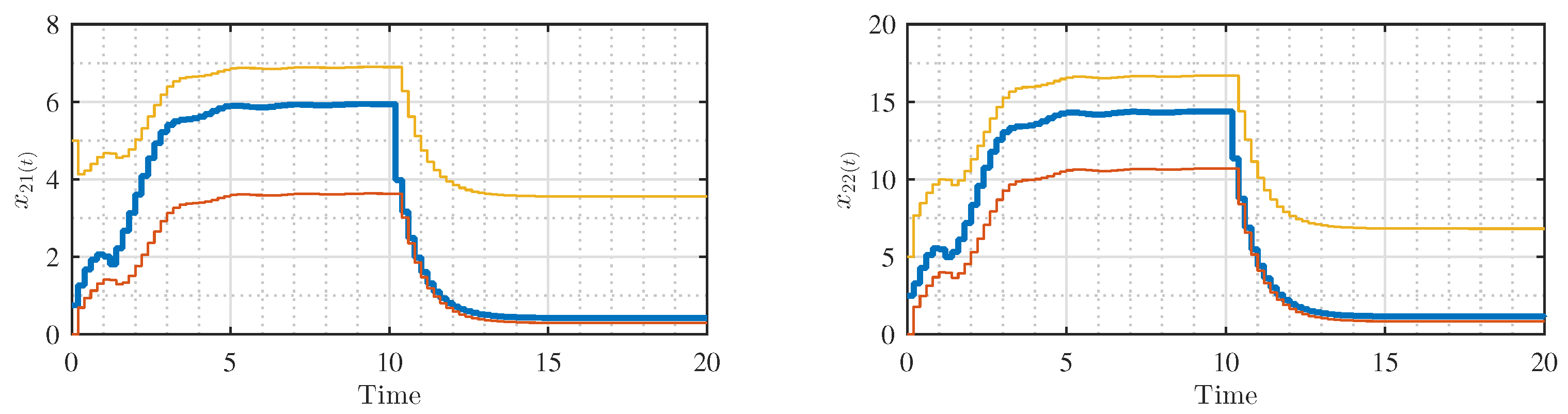
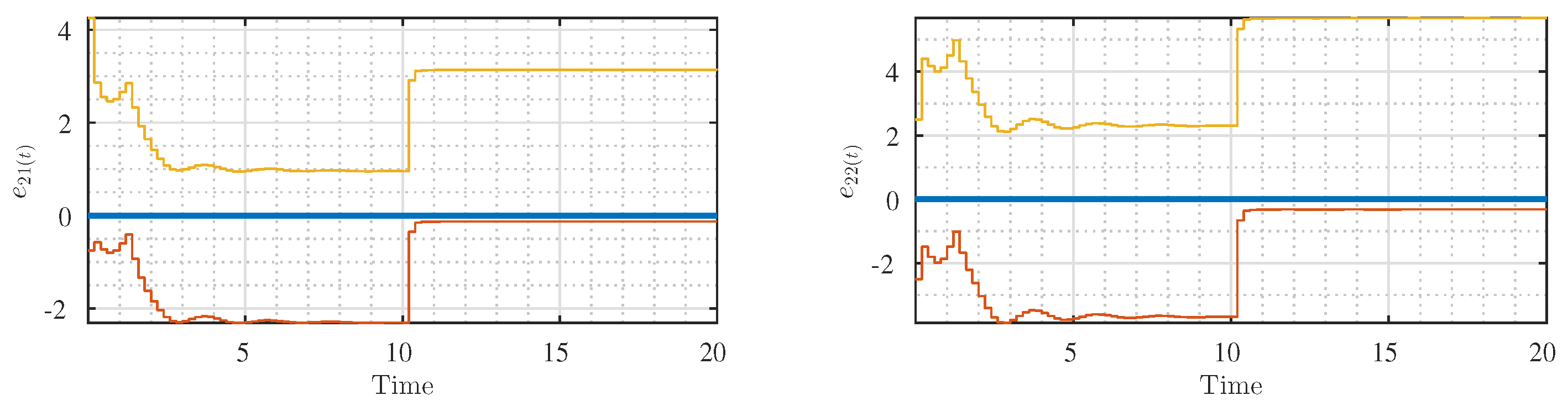
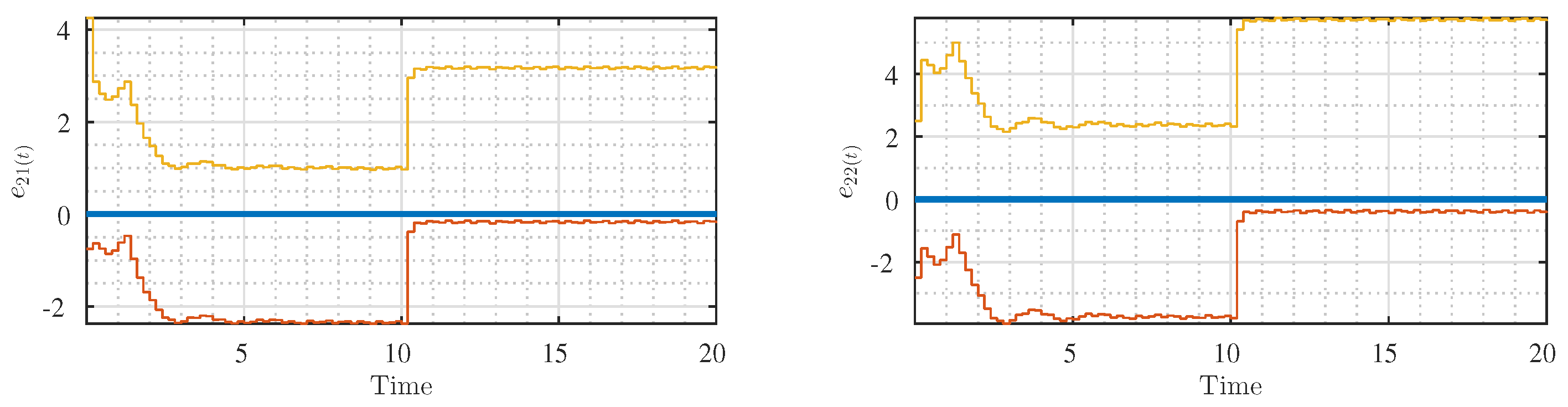
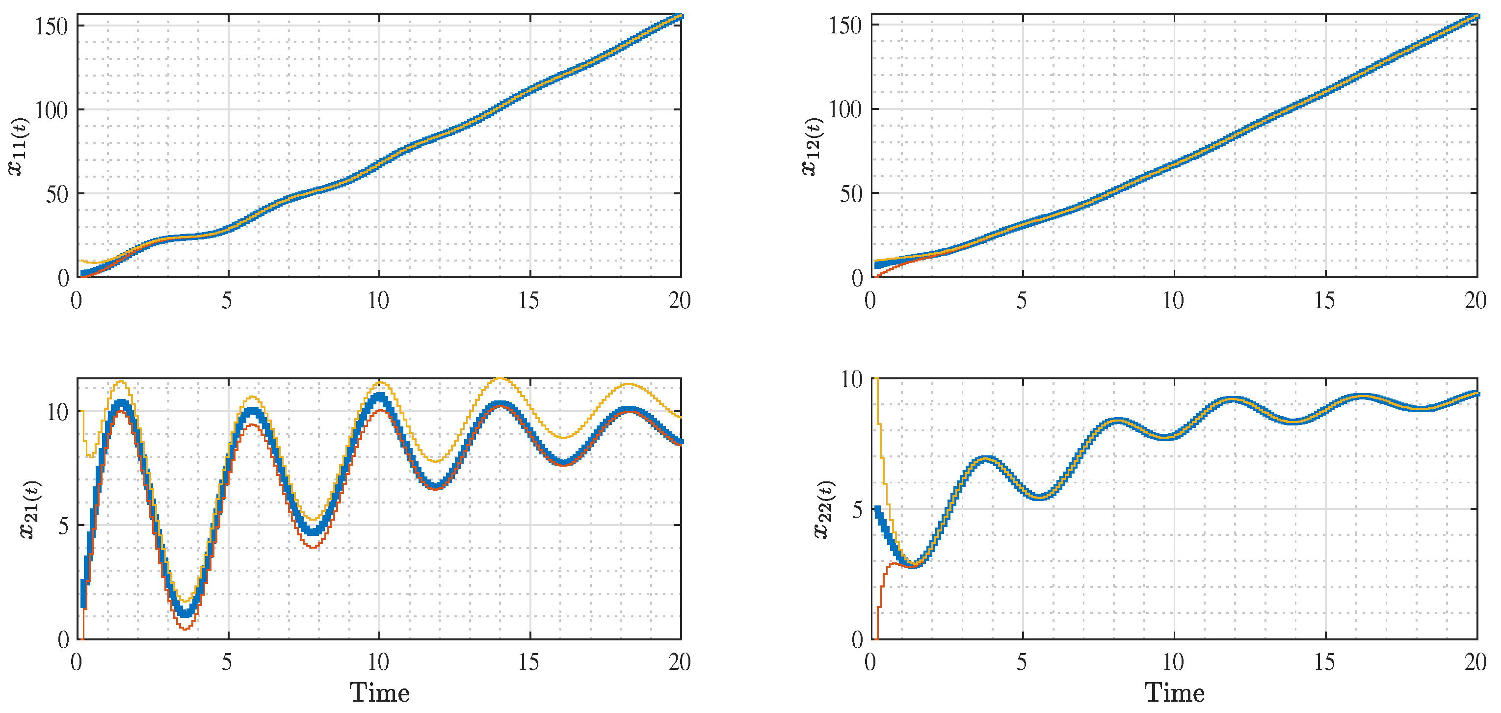
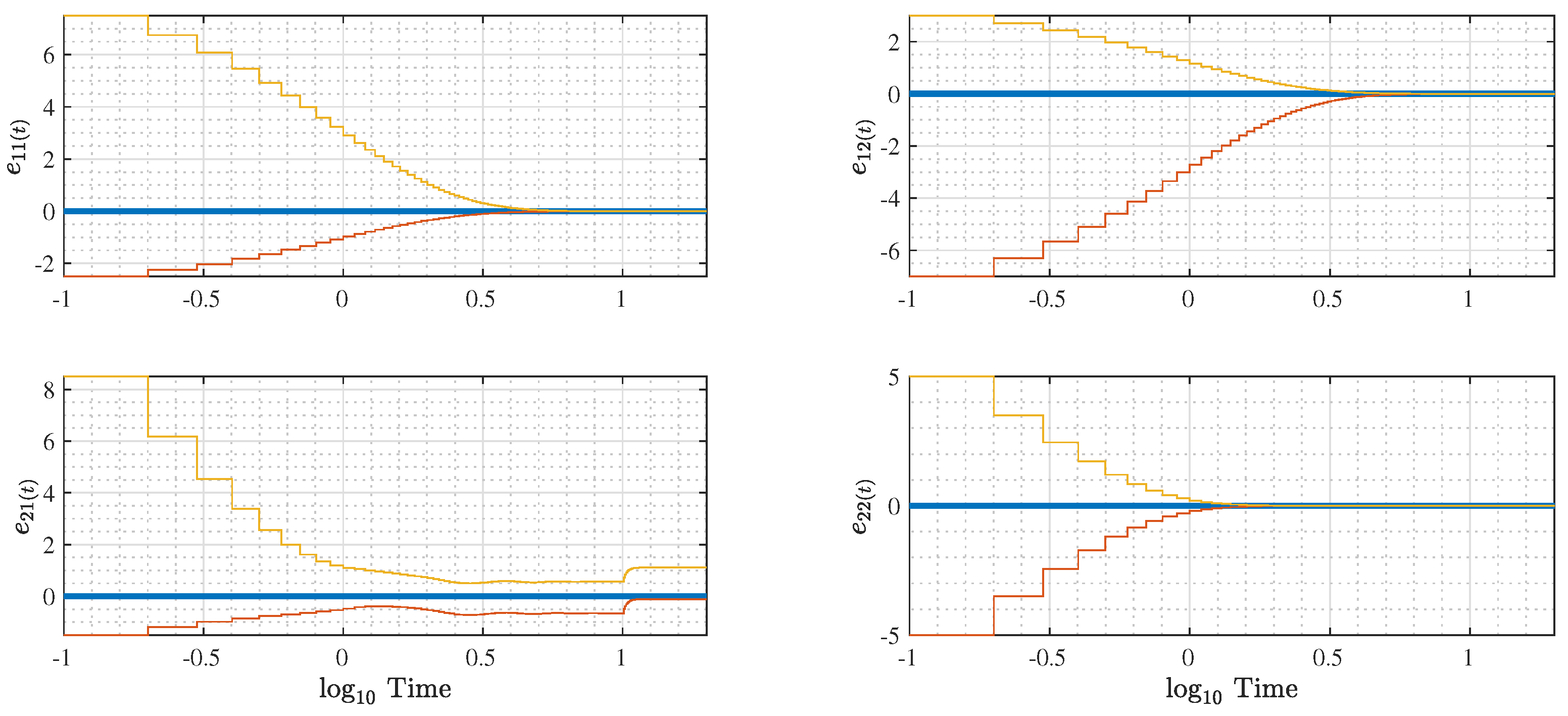
By considering the sampled version of the inputs in Figure 3, the evolution of the true states together with their interval estimates is shown in Figure 10. The estimation error is presented in Figure 11, while the estimation error in the presence of measurement noise is shown in Figure 12. These results verify that the true state trajectory remains bounded between the upper and lower estimates for all $k\in \mathbb{N}$.

5.2.2. Discrete-Time Reduced-Order Interval Observer

To conclude this numerical example, we consider the discrete-time reduced-order interval observer derived in Theorem 4. The observers proposed in (23) and (24) are implemented with the matrix gain ${\mathbf{L}}_{4\mathrm{d}}={\mathbf{A}}_{\mathbf{4}\mathrm{d}}-0.1\mathbf{I}$, which leads to the following matrices of the observers

$$\begin{array}{cc}\hfill {\mathbf{L}}_{4\mathrm{d}}& =\left(\begin{array}{cc}-0.0556& 0.2414\\ 0.4105& 0.4897\end{array}\right),{\mathbf{G}}_1=\left(\begin{array}{cc}0.1& 0\\ 0& 0.1\end{array}\right),{\mathbf{G}}_2=\left(\begin{array}{cc}-0.2319& -1.3416\\ -0.5347& -4.7072\end{array}\right).\hfill \end{array}$$

The interval estimates are shown in Figure 13, while the estimation errors are presented in Figure 14. Finally, the estimation error in the presence of measurement noise is illustrated in Figure 15. These results verify that the reduced-order interval observer preserves the interval-bounding property for the unmeasured state, ${\widehat{\mathbf{x}}}_2^{+}\left[k\right]⪰{\mathbf{x}}_2\left[k\right]⪰{\widehat{\mathbf{x}}}_2^{-}\left[k\right], \forall k\in \mathbb{N}.$

5.3. Mechanical System

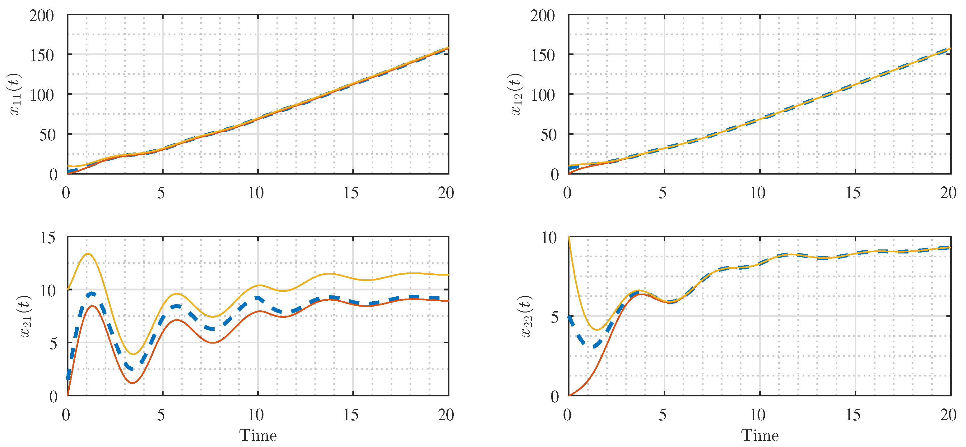
This example illustrates the effectiveness of the proposed full-order interval observer for a mechanical benchmark system composed of two masses connected by a spring and a damper [41] in the presence of bounded inputs and disturbances. Unlike numerical examples, this benchmark highlights the applicability of the proposed interval observer to a physically motivated dynamical system.

The continuous-time linear system is represented by the equations

$$\begin{array}{cc}\hfill {\displaystyle \frac{\mathrm{d}}{\mathrm{d}t}}\left(\begin{array}{c}{z}_1\\ z_2\\ z_3\\ z_4\end{array}\right)=& \left(\begin{array}{cccc}0& 0& 1& 0\\ 0& 0& 0& 1\\ -{\displaystyle \frac{k}{m_1}}& {\displaystyle \frac{k}{m_1}}& -{\displaystyle \frac{c}{m_1}}& {\displaystyle \frac{c}{m_1}}\\ {\displaystyle \frac{k}{m_2}}& -{\displaystyle \frac{k}{m_2}}& {\displaystyle \frac{c}{m_2}}& -{\displaystyle \frac{c}{m_2}}\end{array}\right)\left(\begin{array}{c}{z}_1\\ z_2\\ z_3\\ z_4\end{array}\right)+\left(\begin{array}{c}0\\ 0\\ {\displaystyle \frac{1}{m_1}}\\ 0\end{array}\right)(u\left(t\right)+v\left(t\right))\hfill \\ \hfill \mathbf{y}=& {\left(\begin{array}{cc}{z}_1& z_2\end{array}\right)}^{\top },\hfill \end{array}$$

(28)

where $z_1$ and $z_2$ denote the positions of the masses, while $z_3$ and $z_4$ represent their velocities. Introducing the partition ${\mathbf{x}}_1={\left(z_1{z}_2\right)}^{\top }$ and ${\mathbf{x}}_2={\left(z_3{z}_4\right)}^{\top },$ the system (28) can be rewritten in the form presented in (10), with the matrices

$$\begin{array}{cc}\hfill {\mathbf{A}}_1=& {\mathbf{0}}_{2\times 2},{\mathbf{A}}_2=\left(\begin{array}{cc}-{\displaystyle \frac{k}{m_1}}& {\displaystyle \frac{k}{m_1}}\\ {\displaystyle \frac{k}{m_2}}& -{\displaystyle \frac{k}{m_2}}\end{array}\right),{\mathbf{A}}_3={\mathbf{I}}_2,{\mathbf{A}}_4=\left(\begin{array}{cc}-{\displaystyle \frac{c}{m_1}}& {\displaystyle \frac{c}{m_1}}\\ {\displaystyle \frac{k}{m_2}}& -{\displaystyle \frac{k}{m_2}}\end{array}\right),\hfill \end{array}$$

(29)

where the parameters values are given as $m_1=3,m_2=10,k=5$, and $c=1$. The control input $u\left(t\right)$ and disturbance $v\left(t\right)$ are assumed to be bounded as $5>u\left(t\right)>0,6>v\left(t\right)>0.$ Moreover, the initial conditions for the interval observer are ${\widehat{\mathbf{x}}}_1^{+}\left(0\right)={\left[1010\right]}^{\top }$, ${\widehat{\mathbf{x}}}_2^{+}{\left(0\right)}^{=}{\left[1010\right]}^{\top }$, ${\widehat{\mathbf{x}}}_1^{-}\left(0\right)={\left[00\right]}^{\top }$, and ${\widehat{\mathbf{x}}}_2^{-}{\left(0\right)}^{=}{\left[00\right]}^{\top }$, while the initial state of the plant is chosen as ${\mathbf{x}}_1\left(t\right)={\left[55\right]}^{\top }$ and ${\mathbf{x}}_2\left(t\right)={\left[55\right]}^{\top }$. Thus, these initial states satisfy the interval inequality ${\widehat{\mathbf{x}}}^{+}\left(0\right)⪰\mathbf{x}\left(0\right)⪰{\widehat{\mathbf{x}}}^{-}\left(0\right).$

For this example, we apply the continuous-time full-order interval observer design proposed in Theorem 1 to the plant (28). The selected gains for the interval observer in (11) and (12) are

$$\begin{array}{c}\hfill {\mathbf{L}}_1=2{\mathbf{I}}_2=\left(\begin{array}{cc}2& 0\\ 0& 2\end{array}\right),{\mathbf{L}}_2=\left(\begin{array}{cc}1& 0\\ 0& 1\end{array}\right),{\mathbf{L}}_3={\mathbf{0}}_{2\times 2},{\mathbf{L}}_4={\mathbf{A}}_4+2{\mathbf{I}}_2=\left(\begin{array}{cc}1.6667& 0.3333\\ 0.5& 1.5\end{array}\right).\end{array}$$

The behaviour of the system states and their interval estimates (bounds) are illustrated in Figure 16. It is clear to see that the true state trajectory remains bounded between the upper and lower estimates, that is, ${\widehat{\mathbf{x}}}^{+}\left(t\right)⪰\mathbf{x}\left(t\right)⪰{\widehat{\mathbf{x}}}^{-}\left(t\right), \forall t\ge 0.$ Furthermore, the estimation errors practically converge to a bounded set, given by the presence of bounded perturbations, verifying the theoretical conditions in Theorem 1.

The estimation errors are depicted in Figure 17. There, the time axis is drawn on a logarithmic scale. This scale allows us to show in one diagram the initial conditions for the estimation error as well as the final values that the estimation error achieves. There, one can also see that the upper and lower error bounds monotonically converge toward values close to zero, indicating that the width of the estimation interval decreases over time.

5.4. Mechanical System, Discrete-Time Case

Applying the Euler discretisation, with a sampling period $\tau =0.1$ s, to the plant considered in (28), we obtain the discrete-time model

$$\begin{array}{c}\hfill \mathbf{z}[k+1]={\mathbf{A}}_{\mathbf{d}}\mathbf{z}\left[k\right]+{\mathbf{B}}_{\mathbf{d}}\mathbf{u}\left[k\right]+{\mathbf{D}}_{\mathbf{d}}\mathbf{v}\left[k\right],\end{array}$$

(30)

where the derivative is approximated by $\dot{\mathbf{z}}\left(t\right)\approx {\displaystyle \frac{\mathbf{z}[k+1]-\mathbf{z}\left[k\right]}{\tau }}.$ The matrices are ${\mathbf{A}}_{\mathbf{d}}=\mathbf{I}+\tau \mathbf{A}$, ${\mathbf{B}}_{\mathbf{d}}={\left(\begin{array}{c}0\tau \mathbf{B}\end{array}\right)}^{\top }$, ${\mathbf{D}}_{\mathbf{d}}={\left(\begin{array}{c}0\tau \mathbf{D}\end{array}\right)}^{\top }$. Moreover, $\mathbf{A}$, $\mathbf{B}$, and $\mathbf{D}$ correspond to those defined in (28). Then, the matrices of the sampled system are given by

$$\begin{array}{cc}\hfill {\mathbf{A}}_{\mathbf{d}}& =\left(\begin{array}{cccc}1& 0& 0.1& 0\\ 0& 1& 0& 0.1\\ -0.1667& 0.1667& 0.9667& 0.0333\\ 0.05& -0.05& 0.01& 0.99\end{array}\right),{\mathbf{B}}_{\mathbf{d}}={\mathbf{D}}_{\mathbf{d}}=\left(\begin{array}{c}0\\ 0\\ 0.0333\\ 0\end{array}\right).\hfill \end{array}$$

In this case, the same initial conditions and input signals considered in the continuous-time scenario are used. By applying Theorem 4, the gains of the discrete-time interval observer (19) and (20) are obtained as

$$\begin{array}{cc}\hfill {\mathbf{L}}_{1\mathrm{d}}& =\left(\begin{array}{cc}-0.9& 0\\ 0& -0.9\end{array}\right),{\mathbf{L}}_{2\mathrm{d}}={\mathbf{0}}_{2x2},{\mathbf{L}}_{3\mathrm{d}}={\mathbf{A}}_{3\mathrm{d}}=\left(\begin{array}{cc}0.1& 0\\ 0& 0.1\end{array}\right),\hfill \\ \hfill {\mathbf{L}}_{4\mathrm{d}}& ={\mathbf{A}}_{\mathbf{4}\mathrm{d}}-0.7{\mathbf{I}}_2=\left(\begin{array}{cc}0.2667& 0.0333\\ 0.01& 0.29\end{array}\right).\hfill \end{array}$$

The behaviour of the true unmeasured states, together with their interval estimates, is shown in Figure 18, while the estimation errors are depicted in Figure 19. As expected, the figures confirm the partial ordering between the interval estimates and the true state trajectory for all time instants; that is, ${\widehat{\mathbf{x}}}_2^{+}\left[k\right]⪰{\mathbf{x}}_2\left[k\right]⪰{\widehat{\mathbf{x}}}_2^{-}\left[k\right], \forall k\in \mathbb{N}$.

6. Conclusions

This paper proposed a unified design framework for both full-order and reduced-order interval observers for continuous-time and discrete-time linear systems subject to bounded disturbances and uncertainties, including measurement noise. A central contribution of the proposed methodology is the constructive gain-selection procedure, which enables the estimation error dynamics to be assigned within an admissible class compatible with the observer structure while simultaneously ensuring the required stability and cooperativity properties. For continuous-time systems, this admissible class corresponds to Metzler–Hurwitz error dynamics, whereas for discrete-time systems, it corresponds to element-wise non-negative and Schur-stable error dynamics. This construction guarantees the preservation of the partial ordering between the true state trajectory and the upper and lower interval estimates, while ensuring practical stability of the estimation error dynamics. The unified formulation allows a consistent treatment of both time domains, making the proposed approach suitable for applications in physical systems. Simulation results confirmed the effectiveness and robustness of the proposed observers, demonstrating the interval closure for the state trajectories across various disturbance scenarios. Future research will focus on extending the methodology to nonlinear systems, incorporating time delays, and validating the proposed observers in experimental testbeds for biological processes. A comparative analysis with LMI-based interval observer approaches, considering computational time, interval width, conservatism, and robustness margins, will also be addressed in future work.

References

1. Gouzé, J.L.; Moisan, M.; Bernard, O. A simple improvement of interval asymptotic observers for biotechnological processes. In Proceedings of the ROCOND 2006 Conference, Toulouse, France, 5–7 July 2006. [Google Scholar]
2. Avilés, J.; Moreno, J. Cooperative observers for nonlinear systems. In Proceedings of the Joint 48th IEEE Conference on Decision and Control and 28th Chinese Control Conference, Shanghai, China, 16–18 December 2009; pp. 6125–6130. [Google Scholar]
3. Mazenc, F.; Dinh, T.; Niculescu, S. Robust Interval Observers for Discrete Time Systems of Luenberger Type. In Proceedings of the 2013 IEEE American Control Conference ACC, Washington, DC, USA, 17–19 June 2013; pp. 2484–2489. [Google Scholar]
4. Efimov, D.; Raïssi, T.; Chebotarev, S.; Zolghadri, A. Interval state observer for nonlinear time varying systems. Automatica 2013, 49, 200–205. [Google Scholar] [CrossRef] [Scilit]
5. Avilés, J.D.; Moreno, J.A. Preserving order observers for nonlinear systems. Int. J. Robust. Nonlinear Control 2014, 24, 2153–2178. [Google Scholar] [CrossRef] [Scilit]
6. Avilés, J.D.; Moreno, J.A. Dissipative observers for discrete-time nonlinear systems. J. Frankl. Inst. 2018, 355, 5759–5770. [Google Scholar] [CrossRef] [Scilit]
7. Angeli, D.; Sontag, D. Monotone Control Systems. IEEE Trans. Autom. 2003, 48, 1684–1698. [Google Scholar] [CrossRef] [Scilit]
8. Hirsch, M.; Smith, H. Monotone Dynamical Systems. In Handbook of Differential Equations: Ordinary Differential Equations; Elsevier B. V.: Amsterdam, The Netherlands, 2004; Volume 2, pp. 239–357. [Google Scholar]
9. Gouze, J.L.; Rapaport, A.; Hadj-Sadok, M.Z. Interval observers for uncertain biological systems. Ecol. Model. 2000, 133, 45–56. [Google Scholar] [CrossRef] [Scilit]
10. Alcaraz-Gonzalez, V.; Harmand, J.; Rapaport, A.; Steyer, J.; Gonzalez-Alvarez, V.; Pelayo-Ortiz, C. Software sensors for highly uncertain WWTPS: A new approach based on interval observers. Water Res. 2002, 36, 2515–2524. [Google Scholar] [CrossRef] [Scilit] [PubMed]
11. Bernard, O.; Gouze, J. Closed loop observers bundle for uncertain biotechnological models. J. Process Control 2004, 14, 765–774. [Google Scholar] [CrossRef] [Scilit]
12. Moisan, M.; Bernard, O.; Gouze, J. Near optimal interval observers bundle for uncertain bioreactors. Automatica 2009, 45, 291–295. [Google Scholar] [CrossRef] [Scilit]
13. Mazenc, F.; Bernard, O. Interval observers for linear time-invariant systems with disturbances. Automatica 2011, 47, 140–147. [Google Scholar] [CrossRef] [Scilit]
14. Khan, A.; Xie, W.; Zhang, B.; Liu, L.W. A survey of interval observers design methods and implementation for uncertain systems. J. Frankl. Inst. 2021, 358, 3077–3126. [Google Scholar] [CrossRef] [Scilit]
15. Mazenc, F.; Bernard, O. Asymptotically Stable Interval Observers for Planar systems with Complex Poles. IEEE Trans. Aut. Control 2010, 55, 523–527. [Google Scholar] [CrossRef] [Scilit]
16. Efimov, D.; Perruquetti, W.; Raïssi, T.; Zolghadri, A. Interval Observers for Time-varying Discrete-Time Systems. IEEE Trans. Autom. Control 2013, 58, 3218–3224. [Google Scholar] [CrossRef] [Scilit]
17. Thabet, R.E.H.; Raïssi, T.; Combastel, C.; Efimov, D.; Zolghadri, A. An effective method to interval observer design for time-varying systems. Automatica 2014, 50, 2677–2684. [Google Scholar] [CrossRef] [Scilit]
18. Hirsch, M.; Smith, H. Monotone dynamical systems. Handb. Differ. Equ. Ordinary Differ. Equ. 2005, 2, 239–357. [Google Scholar]
19. Efimov, D.; Perruquetti, W.; Raïssi, T.; Zolghadri, A. On Interval Observer Design for Time-Invariant Discrete-Time Systems. In ECC; IEEE: Zurich, Switzerland, 2013. [Google Scholar]
20. Mazenc, F.; Dinh, T.; Niculescu, S. Interval Observers for Discrete Time Systems. Int. J. Robust. Nonlinear Control 2014, 24, 2867–2890. [Google Scholar] [CrossRef] [Scilit]
21. Wang, Z.; Lim, C.C.; Shen, Y. Interval observer design for uncertain discrete-time linear systems. Syst. Control Lett. 2018, 116, 41–46. [Google Scholar] [CrossRef] [Scilit]
22. Avilés, J.D.; Moreno, J.A. Dissipative interval observer design for discrete-time nonlinear systems. Asian J. Control 2020, 22, 1422–1436. [Google Scholar] [CrossRef] [Scilit]
23. Sergiyenko, O.; Zhirabok, A.; Ibraheem, I.K.; Zuev, A.; Filaretov, V.; Azar, A.T.; Hameed, I.A. Interval observers for discrete-time linear systems with uncertainties. Symmetry 2022, 14, 2131. [Google Scholar] [CrossRef] [Scilit]
24. Xu, F.; Yang, S.; Wang, X. A novel set-theoretic interval observer for discrete linear time-invariant systems. IEEE Trans. Autom. Control 2020, 66, 773–780. [Google Scholar] [CrossRef] [Scilit]
25. Dinh, T.N.; Tran, G.Q.B. Systematic interval observer design for linear systems. Automatica 2025, 180, 112477. [Google Scholar] [CrossRef] [Scilit]
26. Xu, F. An Interval Observer Optimization Design Method for Discrete Linear Time-Invariant Systems. IEEE Control Syst. Lett. 2025, 9, 300–305. [Google Scholar] [CrossRef] [Scilit]
27. Luo, M.; Su, H.; Zheng, W.X. Interval Observer-Based Coordination Control for Discrete-Time Multi-Agent Systems. IEEE Trans. Syst. Man. Cybern. Syst. 2025, 55, 4102–4114. [Google Scholar] [CrossRef] [Scilit]
28. Kailath, T.; Sayed, A.H.; Hassibi, B. Linear Estimation; Prentice Hall: Upper Saddle River, NY, USA, 2000. [Google Scholar]
29. Farina, L.; Rinaldi, S. Positive Linear Systems: Theory and Applications; John Wiley & Sons: Hoboken, NJ, USA, 2000. [Google Scholar]
30. Hirsch, M.; Smith, H. Monotone maps: A review. J. Differ. Equ. Appl. 2005, 11, 379–398. [Google Scholar] [CrossRef] [Scilit]
31. Khalil, H.K.; Grizzle, J.W. Nonlinear Systems; Prentice Hall: Upper Saddle River, NJ, USA, 2002; Volume 3. [Google Scholar]
32. Avilés, J.D.; Moreno, J.A.; Dávila, J.A.; Becerra, G.; Flores, F.; Chávez, C.A.; Márquez, C. Stability radii-based interval observers for discrete-time nonlinear systems. IEEE Access 2021, 10, 3216–3227. [Google Scholar] [CrossRef] [Scilit]
33. Gu, G. Discrete-Time Linear Systems: Theory and Design with Applications; Springer Science & Business Media: Berlin/Heidelberg, Germany, 2012. [Google Scholar]
34. Jiang, Z.P.; Wang, Y. Input-to-state stability for discrete-time nonlinear systems. Automatica 2001, 37, 857–869. [Google Scholar] [CrossRef] [Scilit]
35. Leśniak, A.; Danek, T.; Wojdyła, M. Application of Kalman filter to noise reduction in multichannel data. Schedae Informaticae 2009, 17, 63–73. [Google Scholar] [CrossRef] [Scilit]
36. Stickel, J.J. Data smoothing and numerical differentiation by a regularization method. Comput. Chem. Eng. 2010, 34, 467–475. [Google Scholar] [CrossRef] [Scilit]
37. Chartrand, R. Numerical differentiation of noisy, nonsmooth data. Int. Sch. Res. Not. 2011, 2011, 164564. [Google Scholar] [CrossRef] [Scilit]
38. Van Breugel, F.; Kutz, J.N.; Brunton, B.W. Numerical differentiation of noisy data: A unifying multi-objective optimization framework. IEEE Access 2020, 8, 196865–196877. [Google Scholar] [CrossRef] [Scilit] [PubMed]
39. López-Caamal, F.; Avilés, J.D. A Linear Interval Observer for a Class of Linear Systems of Dimension 2n with n Measurements of the State. In Proceedings of the Memorias del Congreso Nacional de Control Automático, Acapulco de Juárez, Mexico, 25–27 October 2023; pp. 272–277. [Google Scholar]
40. López-Caamal, F.; Avilés, J.D. Reduced Order Interval Observer for Linear Discrete-Time Systems with 2n states and n outputs. In Proceedings of the Memorias del Congreso Nacional de Control Automático, Mexico City, Mexico, 8–11 October 2024; pp. 405–409. [Google Scholar]
41. Zhang, H.; Zhao, S.; Gao, Z. An active disturbance rejection control solution for the two-mass-spring benchmark problem. In Proceedings of the 2016 American Control Conference (ACC); IEEE: Boston, MA, USA, 2016; pp. 1566–1571. [Google Scholar]
Figure 1. Block diagram of the proposed full-order interval observer.
Symmetry 18 00882 g001
Figure 2. Block diagram of the proposed reduced-order interval observer.
Symmetry 18 00882 g002
Figure 3. Inputs to the plant. The left panel depicts in blue the control input u ( t ) , whereas the right one shows the perturbation v ( t ) . The upper and lower bounds of the signals are depicted in yellow and red, respectively.
Symmetry 18 00882 g003
Figure 4. Actual and estimated states of Plant (26) with the continuous-time, full-order observers in Equations (11) and (12). In all panels, the blue line represents the actual state; in turn, the yellow and red lines represent the upper and lower estimates, respectively.
Symmetry 18 00882 g004
Figure 5. Observation errors for the continuous-time, full-order observers in Equations (11) and (12), for the Plant (26). In all panels, the blue line represents zero error; in turn, the yellow and red lines represent the upper and lower estimation error, respectively.
Symmetry 18 00882 g005
Figure 6. Observation errors for the continuous-time, full-order observers in Equations (11) and (12) for the Plant (26), with measurement noise. In all panels, the blue line represents zero error; in turn, the yellow and red lines represent the upper and lower estimation error, respectively.
Symmetry 18 00882 g006
Figure 7. Actual and estimated states of Plant (26) with continuos-time, reduced-order observers in Equations (15) and (16). In all panels, the blue line represents the actual state; in turn, the yellow and red lines represent the upper and lower estimates, respectively.
Symmetry 18 00882 g007
Figure 8. Observation errors for the continuos-time, reduced-order observers in Equations (15) and (16), for Plant (26). In all panels, the blue line represents zero error; in turn, the yellow and red lines represent the upper and lower estimation error, respectively.
Symmetry 18 00882 g008
Figure 9. Observation errors for the continuos-time, reduced-order observers in Equations (15) and (16), for Plant (26), with measurement noise. In all panels, the blue line represents zero error; in turn, the yellow and red lines represent the upper and lower estimation error, respectively.
Symmetry 18 00882 g009
Figure 10. Actual and estimated states of Plant (27) with the discrete-time, full-order observers in Equations (19) and (20). In all panels, the blue line represents the actual state; in turn, the yellow and red lines represent the upper and lower estimates, respectively.
Symmetry 18 00882 g010
Figure 11. Observation errors with the discrete-time, full-order observers in Equations (19) and (20), for Plant (27). In all panels, the blue line represents zero error; in turn, the yellow and red lines represent the upper and lower estimation error, respectively.
Symmetry 18 00882 g011
Figure 12. Observation errors with the discrete-time, full-order observers in Equations (19) and (20), for Plant (27) with measurement noise. In all panels, the blue line represents zero error; in turn, the yellow and red lines represent the upper and lower estimation error, respectively.
Symmetry 18 00882 g012
Figure 13. Actual and estimated states of Plant (27) with the discrete-time, reduced-order observers in Equations (23) and (24). In all panels, the blue line represents the actual state; in turn, the yellow and red lines represent the upper and lower estimates, respectively.
Symmetry 18 00882 g013
Figure 14. Observation errors of reduced-order observers in Equations (23) and (24), for Plant (27). In all panels, the blue line represents zero error; in turn, the yellow and red lines represent the upper and lower estimation error, respectively.
Symmetry 18 00882 g014
Figure 15. Observation errors with the discrete-time, reduced-order observers in Equations (23) and (24), for Plant (27), considering measurement noise. In all panels, the blue line represents zero error; in turn, the yellow and red lines represent the upper and lower estimation error, respectively.
Symmetry 18 00882 g015
Figure 16. States of Plant (28) along with its upper and lower estimates computed with the continuous-time, full-order observers in Equations (11) and (12). In all panels, the blue line represents the actual state; in turn, the yellow and red lines represent the upper and lower estimates, respectively.
Symmetry 18 00882 g016
Figure 17. Estimation error with the continuous-time, full-order interval observer (11) and (12), for Plant (28). In all panels, the blue line represents zero error; in turn, the yellow and red lines represent the upper and lower estimation error, respectively.
Symmetry 18 00882 g017
Figure 18. States of Plant (30), along with its upper and lower estimates via the discrete-time, full-order interval observer in (19) and (20). In all panels, the blue line represents the actual state; in turn, the yellow and red lines represent the upper and lower estimates, respectively.
Symmetry 18 00882 g018
Figure 19. Estimation error of the discrete-time, full-order interval observer (19) and (20), for Plant (30). In all panels, the blue line represents zero error; in turn, the yellow and red lines represent the upper and lower estimation error, respectively.
Symmetry 18 00882 g019
Disclaimer/Publisher’s Note: The statements, opinions and data contained in all publications are solely those of the individual author(s) and contributor(s) and not of MDPI and/or the editor(s). MDPI and/or the editor(s) disclaim responsibility for any injury to people or property resulting from any ideas, methods, instructions or products referred to in the content.