H_∞ Control Designs for Continuous-Time Singular Systems

Abstract

This paper investigates some ${\mathcal{H}}_{\infty }$ control problems for linear continuous-time singular systems. The objective is to design controllers that guarantee the admissibility of the closed-loop system and simultaneously achieve a prescribed ${\mathcal{H}}_{\infty }$ disturbance attenuation level. To this end, a framework based on novel strict LMIs (Linear Matrix Inequalities) is developed using a Lyapunov function approach for the analysis of admissibility and ${\mathcal{H}}_{\infty }$ performance. In particular, an additional scalar parameter $\alpha$ is introduced to generalize the condition reported in previous results in the literature, providing greater flexibility. Then, sufficient LMI conditions are derived for the synthesis of both state-feedback and static output-feedback controllers. Finally, some numerical examples demonstrate the effectiveness of the proposed method.

1. Introduction

The recent interest in singular systems, which combine differential and algebraic equations, is motivated by the increasing complexity of systems to be controlled, due to high variability, high-dimensional dynamics, delays, communication constraints, distributed structures, etc. Under such conditions, traditional control design methods (such as root-locus, pole-placement, or frequency-domain techniques) often prove inadequate. In fact, although differential and algebraic equations are commonly used to model systems for control synthesis, they alone do not accurately represent the dynamical behavior of large-scale and complex systems, which motivates the analysis of singular systems [1]. It is pointed out that singular models arise naturally in these complex systems, due to physical laws, conservation relations, and network interactions [2].

Thus, singular systems constitute an effective framework for describing complex dynamical processes by simultaneously incorporating differential and algebraic equations within a unified mathematical representation. Consequently, they are receiving considerable attention in the control community, leading to multiple recent results (e.g., [3,4,5,6]). These previous results show that the singular representation introduces significant theoretical challenges: the analysis and control of singular systems require the simultaneous treatment of dynamic and algebraic components, making stability analysis, controller synthesis, and performance evaluation substantially more difficult. Moreover, intrinsic characteristics of singular systems, such as admissibility, regularity, and impulse-freeness, further complicate the control design process [7,8].

To synthesize the controller, the concept of $H_{\infty }$ control is used here to deal with the inherent variability of real-life systems: $H_{\infty }$ control was originally introduced by George Zames in the context of optimal sensitivity minimization [9], laying the groundwork for modern robust control theory. Thanks to its disturbance rejection capabilities, the $H_{\infty }$ criterion has been widely used in control design, in particular in distributed control systems. As a result, $H_{\infty }$ controller synthesis has drawn considerable research interest over the past decades (see, for instance, [5,7,8,10,11,12]). Among them, $H_{\infty }$ state-feedback control has been particularly well studied. For instance, Ji et al. [7] proposed a bounded real lemma for singular systems, while Zhang et al. [5] introduced a formulation based on strict LMIs (Linear Matrix Inequalities) for $H_{\infty }$ analysis and synthesis. Subsequently, Chadli et al. [11] and Feng et al. [12] developed improved design conditions aimed at reducing conservatism. Nevertheless, the existing methods still exhibit certain conservative limitations, motivating the search for less conservative and more efficient control design frameworks. It is worth noting that most of the previously mentioned studies focus on discrete-time singular systems. In contrast, the present work generalizes some recent findings reported in [13] for continuous-time singular systems.

The main contribution of this paper is the development of a novel framework for ${\mathcal{H}}_{\infty }$ controller synthesis for continuous-time singular systems. In particular, an additional scalar parameter $\alpha$ is introduced to generalize previous results in the literature, such as Lemma 4 of [14]. When compared with existing approaches [15,16], the incorporation of $\alpha$ increases the flexibility of the proposed formulation, providing reduced conservatism and improved minimum achievable ${\mathcal{H}}_{\infty }$ performance levels. Thus, the specific goals of this paper are the design of state-feedback and static output-feedback ${\mathcal{H}}_{\infty }$ controllers for continuous-time singular systems.

This paper is structured as follows. Section 2 presents the problem formulation, definitions, and some lemmas. Section 3 addresses the admissibility and $H_{\infty }$ control performance and gives the feedback controller design condition. Section 4 extends the feedback design approach. Section 5 provides numerical examples and simulation results. Section 6 concludes with a summary and future research directions.

• Notations:  I is the identity matrix of appropriate dimension. $deg\{·\}$ denotes the polynomial degree. $diag\{·\}$ represents a block-diagonal matrix. The symbol ∗ indicates symmetric terms in a block matrix. ${\mathbb{J}}^T$ is the transpose of $\mathbb{J}$, $Ha\left\{\mathbb{G}\right\}={\mathbb{G}}^T\mathbb{G}$, and $He\left\{\mathbb{G}\right\}=\mathbb{G}+{\mathbb{G}}^T$.

2. Preliminaries and Problem Statement

This section introduces the preliminary concepts and mathematical tools required throughout this paper. In addition, the considered continuous-time singular system model, including the control objective and necessary assumptions, are formally presented.

System Description

Consider a continuous-time singular system described as follows:

$$\left\{\begin{array}{c}\mathbb{E}\dot{x}\left(t\right)=Ax\left(t\right)+\mathbb{B}u\left(t\right)+Fw\left(t\right)\hfill \\ y\left(t\right)=Cx\left(t\right)+\mathbb{D}u\left(t\right)+Hw\left(t\right)\hfill \end{array}\right.,$$

(1)

let $x\left(t\right)\in {\mathbb{R}}^n$ denote the state variable, $u\left(t\right)\in {\mathbb{R}}^q$ the control input, $y\left(t\right)\in {\mathbb{R}}^m$ the controlled output, and $w\left(t\right)\in {\mathbb{R}}^p$ an arbitrary disturbance signal belonging to $L_2[0,\infty )$. The matrix $\mathbb{E}$ may be singular, with rank$\left(\mathbb{E}\right)=r\le n$. Finally, $A,\mathbb{B},C,\mathbb{D},F$ and H are known matrices of appropriate dimensions. To stabilize the considered singular system and achieve the desired ${\mathcal{H}}_{\infty }$ performance, a state-feedback controller of the following form is considered:

$$u\left(t\right)=Kx\left(t\right)$$

(2)

where $K\in {\mathbb{R}}^{q\times n}$ represents the controller gain matrix to be determined. Substituting the state-feedback control law (2) into the original system (1) yields the following closed-loop dynamics:

$$\begin{array}{c}\hfill \left\{\begin{array}{cc}\hfill \mathbb{E}\dot{x}\left(t\right)& = \overline{\mathbf{A}}x\left(t\right)+Fw\left(t\right)\hfill \\ \hfill y\left(t\right)& = \overline{\mathbf{C}}x\left(t\right)+Hw\left(t\right)\hfill \end{array}\right.\end{array}$$

(3)

where $\overline{\mathbf{A}}=A+\mathbb{B}K$ and $\overline{\mathbf{C}}=C+\mathbb{D}K$. Some definitions are now introduced.

Definition 1

([15]). The pair $(\mathbb{E},\overline{\mathbf{A}})$ is defined as follows:

• Regular if $\det (s\mathbb{E}-\overline{\mathbf{A}})$ is not identically zero.
• Impulse-free if $\mathrm{deg}\left(\det (s\mathbb{E}-\overline{\mathbf{A}})\right)=\mathrm{rank}\left(\mathbb{E}\right)$.
• Stable if $Re\left(\lambda (\mathbb{E},\overline{\mathbf{A}})\right)<0$ for all $\lambda (\mathbb{E},\overline{\mathbf{A}})\in \{s\mid \det (s\mathbb{E}-\overline{\mathbf{A}})=0\}$.
• Admissible if it is regular, impulse free, and stable.

Definition 2.

The system (3) considered in this article satisfies the following conditions:

• When $w\left(t\right)=0$, the obtained system (3) is admissible;
• For any non-zero $w\left(t\right)\in L_2[0,\infty )$, given the $H_{\infty }$ performance index γ of the singular system, when the initial condition is zero, ${\int }_0^{+\infty }{y}^T\left(t\right)y\left(t\right)<{\gamma }^2{\int }_0^{+\infty }{w}^T\left(t\right)w\left(t\right)$ can be satisfied.

Lemma 1

([2]). Given any real square matrix $\mathcal{S}$ with appropriate dimension and a scalar $ϵ>0$, the measure $\mu \left(\mathcal{S}\right)$, defined by

$$\mu \left(\mathcal{S}\right)=\underset{ϵ\to 0^{+}}{lim}{\displaystyle \frac{\parallel I+ϵ\mathcal{S}\parallel -1}{ϵ}},$$

has the following properties:

1.

$-\parallel \mathcal{S}\parallel \le \delta \left(\mathcal{S}\right)\le \mu \left(\mathcal{S}\right)\le \parallel \mathcal{S}\parallel$,

2.

$\mu \left(\mathcal{S}\right)={\displaystyle \frac{1}{2}}{\lambda }_{max}(\mathcal{S}+{\mathcal{S}}^T)={\displaystyle \frac{1}{2}}\delta (\mathcal{S}+{\mathcal{S}}^T)$.

where $\delta (·)$ is the generalized spectral abscissa of the pair $(\mathbb{E},\overline{\mathbf{A}})$, defined as

$$\delta (\mathbb{E},\overline{\mathbf{A}})\triangleq \underset{\lambda \in \{s\mid det(s\mathbb{E}-\overline{\mathbf{A}})=0\}}{max}Re\left(\lambda \right).$$

where $\lambda \left(\mathbf{S}\right)$ denotes the eigenvalues of the matrix $\mathbf{S}$, and the usual (non-singular) spectral abscissa is obtained by $\delta \left(\overline{\mathbf{A}}\right)=\delta (I,\overline{\mathbf{A}})$.

Lemma 2

([17]). Given matrices $\mathbb{T}$, $\mathbb{Q}$, $\mathbb{U}$, and $\mathbb{W}$ with compatible dimensions, along with a scalar parameter β, the inequality

$$\mathbb{T}+\mathbb{Q}\mathbb{W}+{\mathbb{W}}^T{\mathbb{Q}}^T<0$$

(4)

is satisfied when the following requirement is met:

$$\left[\begin{array}{cc}\mathbb{T}& \beta \mathbb{Q}+{\mathbb{W}}^T{\mathbb{U}}^T\\ \ast & -\beta \mathbb{U}-\beta {\mathbb{U}}^T\end{array}\right]<0.$$

(5)

3. Main Results

This section presents the main theoretical contributions of this paper. In particular, a new formulation (Lemma 3) is proposed by generalizing Lemma 4 of [14] through the introduction of an additional scalar parameter $\alpha$, which provides greater flexibility in the analysis and synthesis. Based on this formulation, sufficient LMI conditions are derived for the design of both state-feedback and static output-feedback ${\mathcal{H}}_{\infty }$ controllers.

Lemma 3.

For a scalar α and appropriate matrices $\mathbb{T}$, $\mathbb{M}$, $\mathcal{A}$, $\mathbb{G}$, and $\mathcal{P}$, by (6) available (7)

$$\left[\begin{array}{cc}\mathbb{T}+\alpha \mathbb{M}\mathcal{A}+\alpha {\mathcal{A}}^T{\mathbb{M}}^T& \ast \\ \alpha {\mathcal{P}}^T-{\alpha }^2{\mathbb{M}}^T+\mathbb{G}\mathcal{A}& -\alpha \mathbb{G}-\alpha {\mathbb{G}}^T\end{array}\right]<0$$

(6)

$$\mathbb{T}+{\mathcal{A}}^T{\mathcal{P}}^T+\mathcal{P}\mathcal{A}<0.$$

(7)

Proof. 

The inequality (7) can be derived from (6) by applying LMI congruence transformation [14] with the full row rank matrix $\left[\begin{array}{cc}I& {\alpha }^{-1}{\mathcal{A}}^T\end{array}\right]$.    □

Remark 1.

It should be noted that the proposed condition is more general than the one in Lemma 4 of [14], thanks to the introduction of the scalar α. This parameter provides additional flexibility in the solution space, allowing for less conservative results, as illustrated in the example in Section 5.2. In particular, when $\alpha =1$, the proposed condition reduces exactly to Lemma 4 in [14]. Consequently, the proposed formulation generalizes the existing condition and may achieve improved feasibility and better ${\mathcal{H}}_{\infty }$ performance levels.

Remark 2.

The proposed condition (6) can be rewritten as

$$\tilde{Y}\left(\alpha \right)=\underset{{\tilde{Y}}_0}{\underbrace{\left[\begin{array}{cc}\mathbb{T}& \ast \\ \mathbb{G}\mathcal{A}& 0\end{array}\right]}}+\alpha \underset{{\tilde{Y}}_1}{\underbrace{\left[\begin{array}{cc}\mathbb{M}\mathcal{A}+{\mathcal{A}}^T{\mathbb{M}}^T& \ast \\ {\mathcal{P}}^T& -\mathbb{G}-{\mathbb{G}}^T\end{array}\right]}}-{\alpha }^2\underset{{\tilde{Y}}_2}{\underbrace{\left[\begin{array}{cc}0& \ast \\ {\mathbb{M}}^T& 0\end{array}\right]}}<0.$$

(8)

Consider the symmetric matrices

$${\tilde{Y}}_0=\left[\begin{array}{cc}-1& 2\\ 2& 0\end{array}\right],{\tilde{Y}}_1=\left[\begin{array}{cc}0& 1\\ 1& -1\end{array}\right],{\tilde{Y}}_2=\left[\begin{array}{cc}0& 1\\ 1& 0\end{array}\right].$$

For the proposed parameterized condition, choosing $\alpha =2$ yields

$$\tilde{Y}\left(2\right)={\tilde{Y}}_0+2{\tilde{Y}}_1-4{\tilde{Y}}_2=\left[\begin{array}{cc}-1& 2\\ 2& 0\end{array}\right]+\left[\begin{array}{cc}0& 2\\ 2& -2\end{array}\right]-\left[\begin{array}{cc}0& 4\\ 4& 0\end{array}\right]=\left[\begin{array}{cc}-1& 0\\ 0& -2\end{array}\right]\prec 0.$$

However, the conventional condition corresponding to $\alpha =1$ gives

$$\tilde{Y}\left(1\right)={\tilde{Y}}_0+{\tilde{Y}}_1-{\tilde{Y}}_2=\left[\begin{array}{cc}-1& 2\\ 2& 0\end{array}\right]+\left[\begin{array}{cc}0& 1\\ 1& -1\end{array}\right]-\left[\begin{array}{cc}0& 1\\ 1& 0\end{array}\right]=\left[\begin{array}{cc}-1& 2\\ 2& -1\end{array}\right].$$

The characteristic polynomial of $\tilde{Y}\left(1\right)$ is

$$det\left(\left[\begin{array}{cc}-1-\lambda & 2\\ 2& -1-\lambda \end{array}\right]\right)={\lambda }^2+2\lambda -3,$$

whose roots are $\lambda =1$ and $\lambda =-3$. Since $\tilde{Y}\left(1\right)$ possesses a positive eigenvalue, it follows that

$$\tilde{Y}\left(1\right)\nprec 0.$$

Therefore, although the conventional condition is not feasible, the proposed parameterized formulation becomes feasible for a suitable choice of the scalar parameter α. Thus, this example illustrates that the proposed condition can provide a less conservative result than the condition reported in Lemma 4 of [14].

Theorem 1 provides a sufficient condition for the stability analysis of system (1) assuming that the gain matrix K is known.

Theorem 1.

Given a prescribed scalar $\gamma >0$, system (3) is admissible and achieves the minimum $H_{\infty }$ performance level certified by the proposed LMIs if there exist matrices $\mathbb{P}$, X, G, and known controller gain K such that the following matrix inequalities hold:

$${\mathbb{E}}^T\mathbb{P}={\mathbb{P}}^T\mathbb{E}\ge 0,$$

(9)

$$\left[\begin{array}{cc}{\Phi }_1& \ast \\ {\Phi }_2& \mathrm{diag}\left\{-\alpha G-\alpha G^T,-I\right\}\end{array}\right]<0,$$

(10)

where

$$\begin{array}{ccc}& {\Phi }_1=\left[\begin{array}{cc}He\{\alpha XA+\alpha X\mathbb{B}K\}& \ast \\ \alpha F^T{X}^T& -{\gamma }^{2}I\end{array}\right],\hfill & \hfill {\Phi }_2=\left[\begin{array}{cc}\alpha \mathbb{P}-{\alpha }^2{X}^T+GA+G\mathbb{B}K& GF\\ C+\mathbb{D}K& H\end{array}\right].\end{array}$$

Proof. 

First, to establish the admissibility of system (3), we demonstrate that the system is regular and impulse-free. For this, applying the Schur complement to (10) and reformulating the resulting condition into the form of (6) given in Lemma 3 with $\mathbb{M}={\left[\begin{array}{cc}{X}^T& 0\end{array}\right]}^T$, $\mathcal{A}=\left[\begin{array}{cc}\overline{\mathbf{A}}& F\end{array}\right]$, $\mathcal{P}={\left[\begin{array}{cc}\mathbb{P}& 0\end{array}\right]}^T$, $\mathbb{T}=\mathrm{Ha}\left\{\left[\begin{array}{cc}\overline{\mathbf{C}}& H\end{array}\right]\right\}+\mathrm{diag}\left\{0,-{\gamma }^{2}I\right\}$ and $\mathbb{G}=G$, gives the following:

$$\left[\begin{array}{c}{\mathbb{P}}^T\\ 0_{p\times n}\end{array}\right]\left[\begin{array}{cc}\overline{\mathbf{A}}& F\end{array}\right]+\left[\begin{array}{c}{\overline{\mathbf{A}}}^T\\ F^T\end{array}\right]\left[\begin{array}{cc}\mathbb{P}& 0_{n\times p}\end{array}\right]+\mathrm{Ha}\left\{\left[\begin{array}{cc}\overline{\mathbf{C}}& H\end{array}\right]\right\}+\mathrm{diag}\left\{0_n,-{\gamma }^2{I}_p\right\}<0.$$

(11)

From the above inequality, it is clearly to know

$$\left[\begin{array}{c}{\mathbb{P}}^T\\ 0_{p\times n}\end{array}\right]\left[\begin{array}{cc}\overline{\mathbf{A}}& F\end{array}\right]+\left[\begin{array}{c}{\overline{\mathbf{A}}}^T\\ F^T\end{array}\right]\left[\begin{array}{cc}\mathbb{P}& 0_{n\times p}\end{array}\right]+\mathrm{diag}\left\{0_n,-{\gamma }^2{I}_p\right\}<0.$$

(12)

When $w\left(t\right)=0$, pre-multiplying inequality (12) by $\left[\begin{array}{cc}x{\left(t\right)}^T& 0\end{array}\right]$ and post-multiplying by its transpose yields $x^T\left(t\right)\left({\overline{\mathbf{A}}}^T\mathbb{P}+{\mathbb{P}}^T\overline{\mathbf{A}}\right)x\left(t\right)<0$, which is equivalent to

$${\overline{\mathbf{A}}}^T\mathbb{P}+{\mathbb{P}}^T\overline{\mathbf{A}}<0.$$

(13)

To address the three conditions required for the admissibility of the singular system (3), its regularity and impulse-free nature is now established. Since $\mathrm{rank}\left(\mathbb{E}\right)=r<n$, it is assumed that there exist nonsingular matrices M and N satisfying

$$\mathbb{E}=M\left[\begin{array}{cc}{I}_{r\times r}& 0\\ 0& 0\end{array}\right]N,\overline{\mathbf{A}}=M\left[\begin{array}{cc}{\overline{\mathbf{A}}}_1& {\overline{\mathbf{A}}}_2\\ {\overline{\mathbf{A}}}_3& {\overline{\mathbf{A}}}_4\end{array}\right]N,M^T\mathbb{P}{N}^{-1}=\left[\begin{array}{cc}{\mathbb{P}}_1& {\mathbb{P}}_2\\ {\mathbb{P}}_3& {\mathbb{P}}_4\end{array}\right],$$

(14)

where the partition is consistent with that of $\overline{\mathbf{A}}$. From (9) and (14), it follows that ${\mathbb{P}}_2=0$ and ${\mathbb{P}}_1>0$. Observing (13) and applying Lemma 1, we obtain

$$\delta \left({\overline{\mathbf{A}}}^T\mathbb{P}\right)\le \mu \left({\overline{\mathbf{A}}}^T\mathbb{P}\right)={\displaystyle \frac{1}{2}}{\lambda }_{max}\left({\mathbb{P}}^T\overline{\mathbf{A}}+{\overline{\mathbf{A}}}^T\mathbb{P}\right)$$

(15)

Therefore, ${\overline{\mathbf{A}}}^T\mathbb{P}$ is nonsingular, indicating that $\mathbb{P}$ is nonsingular as well. Pre- and post-multiplying (13) by $N^{-T}$ and $N^{-1}$, respectively, and employing the relations in (14) yields the inequality

$$\left[\begin{array}{cc}{\Theta }_1& {\Theta }_2\\ {\Theta }_2^T& {\Theta }_3\end{array}\right]<0,$$

(16)

where ${\Theta }_1=He\left({\overline{\mathbf{A}}}_1^T{\mathbb{P}}_1+{\overline{\mathbf{A}}}_3^T{\mathbb{P}}_3\right),{\Theta }_2={\overline{\mathbf{A}}}_3^T{\mathbb{P}}_4+{\mathbb{P}}_1^T{\overline{\mathbf{A}}}_2+{\mathbb{P}}_3^T{\overline{\mathbf{A}}}_4,{\Theta }_3=He\left({\overline{\mathbf{A}}}_4^T{\mathbb{P}}_4\right).$

From (16), it follows that

$$He\left({\overline{\mathbf{A}}}_4^T{\mathbb{P}}_4\right)<0.$$

(17)

The above inequality, together with Lemma 1, yields

$$\delta \left({\mathbb{P}}_4^T{\overline{\mathbf{A}}}_4\right)\le \mu \left({\mathbb{P}}_4^T{\overline{\mathbf{A}}}_4\right)={\displaystyle \frac{1}{2}}{\lambda }_{max}\left({\overline{\mathbf{A}}}_4^T{\mathbb{P}}_4+{\mathbb{P}}_4^T{\overline{\mathbf{A}}}_4\right).$$

(18)

So ${\mathbb{P}}_4^T{\overline{\mathbf{A}}}_4$ is nonsingular, which implies ${\overline{\mathbf{A}}}_4$ is nonsingular too. In this case, one has

$$\begin{array}{cc}\hfill \det \left(M^{-1}(s\mathbb{E}-\overline{\mathbf{A}})N^{-1}\right)& =\det (s{I}_r-{\overline{\mathbf{A}}}_1+{\overline{\mathbf{A}}}_2{\overline{\mathbf{A}}}_4^{-1}{\overline{\mathbf{A}}}_3)\times \det (-{\overline{\mathbf{A}}}_4),\hfill \end{array}$$

(19)

where for any scalar “s”, which is not equal to the eigenvalue of matrix $({\overline{\mathbf{A}}}_1-{\overline{\mathbf{A}}}_2{\overline{\mathbf{A}}}_4^{-1}{\overline{\mathbf{A}}}_3)$ is selected, therefore,

$$\det (s{I}_r-{\overline{\mathbf{A}}}_1+{\overline{\mathbf{A}}}_2{\overline{\mathbf{A}}}_4^{-1}{\overline{\mathbf{A}}}_3)\ne 0,$$

and

$$\det \left(M^{-1}(s\mathbb{E}-\overline{\mathbf{A}})N^{-1}\right)\ne 0.$$

Thus, by Definition 1, the pair $(\mathbb{E},\overline{\mathbf{A}})$ is regular, meaning that system (3) is regular. Moreover, from (19), it can be concluded that

$$deg\left(\det (s\mathbb{E}-\overline{\mathbf{A}})\right)=r=rank\left(\mathbb{E}\right),$$

which implies that the pair $(\mathbb{E},\overline{\mathbf{A}})$ is impulse-free; consequently, system (3) is impulse-free. Therefore, condition (10) in Theorem 1 guarantees both the regularity and impulse-free state of system (3). To establish full admissibility, the stability of system (3) must still be demonstrated. For this, the following Lyapunov function is used:

$$\mathbb{V}\left(x\left(t\right)\right)=x^T\left(t\right){\mathbb{E}}^T\mathbb{P}x\left(t\right),{\mathbb{E}}^T\mathbb{P}={\mathbb{P}}^T\mathbb{E}\ge 0.$$

(20)

Then,

$$\begin{array}{cc}\hfill \dot{\mathbb{V}}\left(x\left(t\right)\right)& ={\dot{x}}^T\left(t\right){\mathbb{E}}^T\mathbb{P}x\left(t\right)+x^T\left(t\right){\mathbb{P}}^T\mathbb{E}\dot{x}\left(t\right)\hfill \\ \hfill & ={\psi }^T\left(t\right)\left(\left[\begin{array}{c}{\mathbb{P}}^T\\ 0\end{array}\right]\left[\begin{array}{cc}\overline{\mathbf{A}}& F\end{array}\right]+\left[\begin{array}{c}{\overline{\mathbf{A}}}^T\\ F^T\end{array}\right]\left[\begin{array}{cc}\mathbb{P}& 0\end{array}\right]\right)\psi \left(t\right)\hfill \end{array}$$

(21)

where $\psi \left(t\right)={\left[x^T\left(t\right)w^T\left(t\right)\right]}^T$. When $w\left(t\right)=0$, it follows from (13) that $\dot{\mathbb{V}}\left(x\left(t\right)\right)<0$. Thus, the stability of system (3) is established. By Definition 1, system (3) is therefore admissible. Considering the case $w\left(t\right)\ne 0$, system (3) and Equation (21) imply

$$\begin{array}{cc}\hfill \mathbb{J}\left(t\right)& =\dot{\mathbb{V}}\left(x\left(t\right)\right)+y^T\left(t\right)y\left(t\right)-{\gamma }^2{w}^T\left(t\right)w\left(t\right)\hfill \\ \hfill & ={\psi }^T\left(t\right)\left(\left[\begin{array}{c}{\mathbb{P}}^T\\ 0\end{array}\right]\left[\begin{array}{cc}\overline{\mathbf{A}}& F\end{array}\right]+\left[\begin{array}{c}{\overline{\mathbf{A}}}^T\\ F^T\end{array}\right]\left[\begin{array}{cc}\mathbb{P}& 0\end{array}\right]+\mathrm{Ha}\left\{\left[\begin{array}{cc}\overline{\mathbf{C}}& H\end{array}\right]\right\}+diag\left\{0,-{\gamma }^{2}I\right\}\right)\psi \left(t\right).\hfill \end{array}$$

(22)

From inequality (11), we can know $\mathbb{J}\left(t\right)<0$ for any $\psi \left(t\right)\ne 0$. When the initial condition is zero and $\mathbb{V}\left(x\right(\infty \left)\right)>0$, it is clear that ${\int }_0^{+\infty }{y}^T\left(t\right)y\left(t\right)<{\gamma }^2{\int }_0^{+\infty }{w}^T\left(t\right)w\left(t\right)$ with any non-zero $w\left(t\right)\in L_2[0,\infty )$. Clearly, the desired $H_{\infty }$ performance $\gamma$ of system (3) is achieved. This concludes the proof.    □

Remark 3.

Formula (10) provides a criterion for analyzing the admissibility of system (3) with $H_{\infty }$ performance. However, when K is unknown, the condition contains nonlinear terms, including the coupling terms $X\mathbb{B}K$ and $G\mathbb{B}K$. These terms render the condition non-convex, so it cannot be directly solved using the LMI toolbox in MATLAB. To address the controller design problem in (2), (10) in Theorem 1 is linearized using LMI techniques, to derive a tractable design condition for the controller.

Remark 4.

The LMIs in this paper involve a full Lyapunov matrix $\mathbb{P}$ satisfying (10) and (9). When solved using standard interior-point LMI solvers, the computational complexity scales unfavorably with the state dimension n. The fact that semidefinite programming is class P-Complete, makes large-scale LMI problems inherently challenging to solve in parallel [18]. For systems with hundreds of states, existing algorithms typically fail due to memory limitations [18]. Several approaches exist to address this limitation. For large-scale descriptor systems, there are model reduction techniques [19]. Alternatively, specialized solvers such as DSDP (Dual-Scaling Algorithm for Semidefinite Programming) exploit low-rank structure and sparsity to achieve scalable parallel performance [20,21,22]. More recent results employ ADMM (Alternating Direction Method of Multipliers) distributed synthesis, where the LMI size per subsystem depends only on local information [23]. Extending the proposed conditions to exploit such structure is a promising direction for future work.

The design condition for the controller gain matrix in (2) is now provided to guarantee that system (3) meets the required $H_{\infty }$ performance. Moreover, the following theorem solves the problem discussed in Remark 3 by applying a decoupling method to transform the nonlinear matrix inequality into a standard LMI formulation.

Theorem 2.

Consider the continuous singular system described in (1) with a given scalar $\gamma >0$. There exists a state-feedback controller of the form (2) such that the closed-loop system in (3) is admissible and achieves the minimum $H_{\infty }$ performance level certified by the proposed LMIs, that is if there exist two known scalars α and β and matrices $P>0$, Q, X, G, V, and U satisfy the following matrix inequality:

$$\left[\begin{array}{ccc}{\Xi }_1& \ast & \ast \\ {\Xi }_2& {\Xi }_3& \ast \\ {\Xi }_4& {\Xi }_5& -\beta U-\beta U^T\end{array}\right]<0,$$

(23)

with $Z\in {\mathbb{R}}^{n,(n-r)}$ and ${\mathbb{E}}^{T}Z=0$, where

$$\begin{array}{ccc}\hfill & {\Xi }_1=\left[\begin{array}{cc}He\{\alpha XA+\mathbb{B}V\}& \ast \\ \alpha F^T{X}^T& -{\gamma }^{2}I\end{array}\right],\hfill & \hfill {\Xi }_2=\left[\begin{array}{cc}\alpha (P\mathbb{E}+ZQ)-{\alpha }^2{X}^T+GA+\mathbb{B}V& GF\\ C+\mathbb{D}V& H\end{array}\right],\end{array}$$

$$\begin{array}{ccc}\hfill & {\Xi }_3=diag\left\{-\alpha G-\alpha G^T,-I\right\},\hfill & \hfill {\Xi }_4=\left[V+\beta {(\alpha X\mathbb{B}-\mathbb{B}U)}^{T}0\right],\\ \hfill & {\Xi }_5=\left[\beta {(G\mathbb{B}-\mathbb{B}U)}^T\beta {(\mathbb{D}-\mathbb{D}U)}^T\right].\hfill \end{array}$$

Then, the gain matrix is $K=U^{-1}V$.

Proof. 

To derive an LMI condition, we begin by applying the transformation $\mathbb{P}=P\mathbb{E}+ZQ$, where $P>0$ and Q are matrices, and $Z\in {\mathbb{R}}^{n,(n-r)}$ satisfies ${\mathbb{E}}^{T}Z=0$, as proposed in [15]. Then, by applying this transformation to inequality (10) and isolating the relevant terms, we arrive at the following inequality

$$\Theta +\mathbb{V}K\mathbb{R}+{\mathbb{R}}^T{K}^T{\mathbb{V}}^T<0$$

(24)

where

$$\begin{array}{c}\hfill \Theta =\left[\begin{array}{cc}{\Theta }_1& \ast \\ {\Theta }_2& {\Xi }_3\end{array}\right],\end{array}$$

$$\begin{array}{c}\hfill {\Theta }_1=\left[\begin{array}{cc}\alpha XA+\alpha A^T{X}^T& \ast \\ \alpha F^T{X}^T& -{\gamma }^{2}I\end{array}\right],{\Theta }_2=\left[\begin{array}{cc}\alpha (P\mathbb{E}+ZQ)-{\alpha }^2{X}^T+GA& GF\\ C& H\end{array}\right],\end{array}$$

$$\begin{array}{cc}\hfill & \mathbb{V}={\left[\begin{array}{cccc}\alpha {\mathbb{B}}^T{X}^T\hfill & 0\hfill & {\mathbb{B}}^T{G}^T\hfill & {\mathbb{D}}^T\hfill \end{array}\right]}^T,\mathbb{R}=\left[\begin{array}{cccc}I\hfill & 0\hfill & 0\hfill & 0\hfill \end{array}\right].\hfill \end{array}$$

Inspired by the design methodology proposed in [24], consider a nonsingular matrix variable U and a matrix variable V. By defining $K=U^{-1}V$, the following relations can be derived:

$$X\mathbb{B}K=(X\mathbb{B}-\mathbb{B}U)U^{-1}V+\mathbb{B}V,$$

(25)

$$G\mathbb{B}K=(G\mathbb{B}-\mathbb{B}U)U^{-1}V+\mathbb{B}V,$$

(26)

$$\mathbb{D}K=(\mathbb{D}-\mathbb{D}U)U^{-1}V+\mathbb{D}V.$$

(27)

Using (25)–(27), inequality (24) can be equivalently rewritten as follows:

$$\stackrel{\mathbb{T}}{\overbrace{{\rm Y}}}+sym\left(\underset{\mathbb{Q}}{\underbrace{⨿}}\underset{\mathbb{W}}{\underbrace{U^{-1}V\mathbb{R}}}\right)<0,$$

(28)

where

$$\begin{array}{cc}\hfill {\rm Y}& =\left[\begin{array}{cc}{\Xi }_1& \ast \\ {\Xi }_2& {\Xi }_3\end{array}\right],\hfill \\ \hfill ⨿& ={\left[\begin{array}{cccc}{(\alpha X\mathbb{B}-\mathbb{B}U)}^T\hfill & 0\hfill & {(G\mathbb{B}-\mathbb{B}U)}^T\hfill & {(\mathbb{D}-\mathbb{D}U)}^T\hfill \end{array}\right]}^T.\hfill \end{array}$$

Finally, by applying Lemma 2 to (28) it follows that (28) guarantees (23). Hence, the system (3) is admissible with the desired $H_{\infty }$ performance. The proof is complete.    □

Remark 5.

Theorem 2 provides a solvability condition for the $H_{\infty }$ control problem. To further illustrate the advantage of the proposed approach, we introduce the following optimization problem:

$$min\mu \mathit{subject}\mathit{to}\mathit{LMI}\left(23\right)\mathit{with}\mu ={\gamma }^2.$$

Consequently, the minimal achievable $H_{\infty }$ performance level is given by ${\gamma }_{min}=\sqrt{{\mu }_{min}}$.

Remark 6.

The conditions presented in Theorem 2 are formulated as LMIs once the scalar parameters α and β are fixed. Therefore, the determination of suitable values for these parameters can be carried out through an optimization procedure (Algorithm 1). In particular, an iterative search algorithm based on the fminsearch function available in MATLAB’s Optimization Toolbox may be employed to compute the values of α and β that optimize the desired performance criterion [25,26,27]. After obtaining these parameters, the feasibility problem associated with Theorem 2 can be efficiently solved using the MATLAB LMI Control Toolbox [28].

Algorithm 1 Determination of the scalar parameters $\alpha$ and $\beta$

1: Choose initial values ${\alpha }_0$ and ${\beta }_0$. 2: Define the objective function associated with Theorem 2, for instance the minimum certified $H_{\infty }$ performance level. 3: Use the MATLAB function fminsearch to solve $$({\alpha }^{\star },{\beta }^{\star })=\arg \underset{\alpha ,\beta }{min}J(\alpha ,\beta ),$$    where $J(\alpha ,\beta )$ denotes the selected performance criterion. 4: for each candidate pair $(\alpha ,\beta )$ do 5:     Substitute $\alpha$ and $\beta$ into the LMIs of Theorem 2. 6:     Solve the resulting LMIs using the MATLAB LMI Control Toolbox. 7:     if the LMIs are feasible then 8:              Compute the corresponding controller matrices and the certified $H_{\infty }$ performance level. 9:     else 10:             Assign a large penalty value to $J(\alpha ,\beta )$. 11:    end if 12: end for 13: Return the optimal values ${\alpha }^{\star }$ and ${\beta }^{\star }$ together with the corresponding feasible solution. 14: Fix $\alpha ={\alpha }^{\star }$ and $\beta ={\beta }^{\star }$ in the LMIs of Theorem 2. 15: Solve the resulting LMIs to compute the corresponding minimum certified $H_{\infty }$ performance level and the associated control gain. 16: Return the optimal parameters $({\alpha }^{\star },{\beta }^{\star })$, the minimum certified performance level, and the corresponding controller gain.

4. H_∞ Static Output Design

The design conditions for the output-feedback controller are presented in the main results that follow.

Consider the following system

$$\begin{array}{c}\hfill \left\{\begin{array}{cc}\hfill \mathbb{E}\dot{x}\left(t\right)& = Ax\left(t\right)+\mathbb{B}u\left(t\right)+\mathbb{F}w\left(t\right)\hfill \\ \hfill z\left(t\right)& = Jx\left(t\right)+\mathbb{M}w\left(t\right)\hfill \\ \hfill y\left(t\right)& = Cx\left(t\right)+\mathbb{D}u\left(t\right)+\mathbb{H}w\left(t\right),\hfill \end{array}\right.\end{array}$$

(29)

where $z\left(t\right)\in {\mathbb{R}}^l$ is the measured output. J, $\mathbb{M}$, $\mathbb{B}$, $\mathbb{F}$, $\mathbb{D}$, and $\mathbb{H}$ are known matrices of appropriate dimensions, $\mathbb{B}$ is full rank, and other notation is consistent with system (1).

Then, the output-feedback controller is given by

$$u\left(t\right)=\mathbb{K}z\left(t\right)$$

(30)

where $\mathbb{K}\in {\mathbb{R}}^{q\times l}$ is the controller gain matrix. This yields the closed-loop system

$$\begin{array}{c}\hfill \left\{\begin{array}{cc}\hfill \mathbb{E}\dot{x}\left(t\right)& = {\mathbb{A}}_{1}x\left(t\right)+{\mathbb{B}}_{1}w\left(t\right)\hfill \\ \hfill y\left(t\right)& = {\mathbb{C}}_{1}x\left(t\right)+{\mathbb{H}}_{1}w\left(t\right),\hfill \end{array}\right.\end{array}$$

(31)

where ${\mathbb{A}}_1=A+\mathbb{B}\mathbb{K}J, {\mathbb{B}}_1=\mathbb{F}+\mathbb{B}\mathbb{K}\mathbb{M}, {\mathbb{C}}_1=C+\mathbb{D}\mathbb{K}J$ and ${\mathbb{H}}_1=\mathbb{H}+\mathbb{D}\mathbb{K}\mathbb{M}$.

• The next theorem addresses the design of a static output-feedback controller based on the conditions established in Theorem 1.

Theorem 3.

Consider the continuous singular system described in (1) with a given scalar $\gamma >0$. There exists a static output-feedback controller of the form (30) such that the closed-loop system in (31) is admissible and achieves the minimum $H_{\infty }$ performance level certified by the proposed LMIs if there exist two known scalars α and β, and matrices $\widehat{P}>0$, $\widehat{Q}$, $\widehat{X}$, $\widehat{G}$, $\widehat{V}$, and $\widehat{U}$ satisfy the following matrix inequality:

$$\left[\begin{array}{ccc}{\Lambda }_1& \ast & \ast \\ {\Lambda }_2& {\Lambda }_3& \ast \\ {\Lambda }_4& {\Lambda }_5& -\beta \widehat{U}-\beta {\widehat{U}}^T\end{array}\right]<0,$$

(32)

with $\widehat{Z}\in {\mathbb{R}}^{n,(n-r)}$ and ${\mathbb{E}}^T\widehat{Z}=0$, where

$$\begin{array}{cc}\hfill {\Lambda }_1& =\left[\begin{array}{cc}He\{\alpha \widehat{X}A+\mathbb{B}\widehat{V}J\}& \ast \\ \alpha {\mathbb{F}}^T{\widehat{X}}^T+{\mathbb{M}}^T{\widehat{V}}^T{\mathbb{B}}^T& -{\gamma }^{2}I\end{array}\right],\hfill \end{array}$$

$$\begin{array}{cc}\hfill {\Lambda }_2& =\left[\begin{array}{cc}\alpha (\widehat{P}\mathbb{E}+\widehat{Z}\widehat{Q})-{\alpha }^2{\widehat{X}}^T+\widehat{G}A+\mathbb{B}\widehat{V}J& \widehat{G}\mathbb{F}+\mathbb{B}\widehat{V}\mathbb{M}\\ C+\mathbb{D}\widehat{V}J& \mathbb{H}+\mathbb{D}\widehat{V}\mathbb{M}\end{array}\right],\hfill \end{array}$$

$$\begin{array}{cc}{\Lambda }_3=\mathrm{diag}\left\{-\alpha \widehat{G}-\alpha {\widehat{G}}^T,-I\right\},\hfill & \hfill {\Lambda }_4=\left[\begin{array}{cc}\widehat{V}J+\beta {(\alpha \widehat{X}\mathbb{B}-\mathbb{B}\widehat{U})}^T& \widehat{V}\mathbb{M}\end{array}\right],\\ {\Lambda }_5=\left[\begin{array}{cc}\beta {(\widehat{G}\mathbb{B}-\mathbb{B}\widehat{U})}^T& \beta {(\mathbb{D}-\mathbb{D}\widehat{U})}^T\end{array}\right].\hfill & \end{array}$$

Then, the gain matrix is $\mathbb{K}={\widehat{U}}^{-1}\widehat{V}$.

Proof. 

The analysis procedure can be derived from Theorem 1 by replacing the matrices $\overline{\mathbf{A}}$, F, $\overline{\mathbf{C}}$, and H in (3) with ${\mathbb{A}}_1$, ${\mathbb{B}}_1$, ${\mathbb{C}}_1$, and ${\mathbb{H}}_1$ in (31), respectively. Consequently, the conditions of Theorem 1 become

$${\mathbb{E}}^T\mathbb{P}={\mathbb{P}}^T\mathbb{E}\ge 0$$

(33)

$$\left[\begin{array}{cc}{\mathsf{\Pi }}_1& \ast \\ {\mathsf{\Pi }}_2& \mathrm{diag}\left\{-\alpha \widehat{G}-\alpha {\widehat{G}}^T,-I\right\}\end{array}\right]<0,$$

(34)

where

$$\begin{array}{c}\hfill {\mathsf{\Pi }}_1=\left[\begin{array}{cc}He\{\alpha \widehat{X}A+\alpha \widehat{X}\mathbb{B}\mathbb{K}J\}& \ast \\ \alpha {\mathbb{F}}^T{\widehat{X}}^T+\alpha {\mathbb{M}}^T{\mathbb{K}}^T{\mathbb{B}}^T{\widehat{X}}^T& -{\gamma }^{2}I\end{array}\right],\end{array}$$

$$\begin{array}{c}\hfill {\mathsf{\Pi }}_2=\left[\begin{array}{cc}\alpha \mathbb{P}-{\alpha }^2{\widehat{X}}^T+\widehat{G}A+\widehat{G}\mathbb{B}\mathbb{K}J& \widehat{G}\mathbb{F}+\widehat{G}\mathbb{B}\mathbb{K}\mathbb{M}\\ C+\mathbb{D}\mathbb{K}J& \mathbb{H}+\mathbb{D}\mathbb{K}\mathbb{M}\end{array}\right].\end{array}$$

In order to derive an LMI condition, we consider the transformation $\mathbb{P}=\widehat{P}\mathbb{E}+\widehat{Z}\widehat{Q}$, where $\widehat{P}>0$ and $\widehat{Q}$ are matrices, and $\widehat{Z}\in {\mathbb{R}}^{n,(n-r)}$ satisfies ${\mathbb{E}}^T\widehat{Z}=0$, following the approach in [15]. Then, adapting the previous transformations to the output-feedback control case, the following is obtained:

$$\begin{array}{cc}\hfill \uplus \mathbb{B}\mathbb{K}⊛& =(\uplus \mathbb{B}-\mathbb{B}\widehat{U}){\widehat{U}}^{-1}\widehat{V}⊛+\mathbb{B}\widehat{V}⊛,\mathrm{where}\uplus =\{\widehat{X},\widehat{G}\}\mathrm{and}⊛=\{\mathbb{M},J\}\hfill \end{array}$$

(35)

$$\begin{array}{cc}\hfill \mathbb{D}\mathbb{K}⊛& =(\mathbb{D}-\mathbb{D}\widehat{U}){\widehat{U}}^{-1}\widehat{V}⊛+\mathbb{D}\widehat{V}⊛.\hfill \end{array}$$

(36)

Then, following the same arguments as in the proof of Theorem 2 (see Proof 3), Theorem 3 is established. □

Remark 7.

To allow a direct comparison with the results of [15], the matrices C, $\mathbb{M}$, $\mathbb{D}$, and $\mathbb{H}$ in (29) are set to zero, and the control law is $u\left(t\right)=\mathbb{K}z\left(t\right)$. The obtained closed-loop follows from (29) as

$$\begin{array}{c}\hfill \left\{\begin{array}{cc}\hfill \mathbb{E}\dot{x}\left(t\right)& = (A+\mathbb{B}\mathbb{K}J)x\left(t\right)+\mathbb{F}w\left(t\right)\hfill \\ \hfill z\left(t\right)& = Jx\left(t\right),\hfill \end{array}\right.\end{array}$$

(37)

which coincides with the formulation in [15].

According to Theorem 3, we can easily obtain the following result of the closed-loop system (37).

Corollary 1.

Consider the continuous singular system described in (1) with a given scalar $\gamma >0$. There exists a static output-feedback controller of the form (30) such that the closed-loop system (37) is admissible and achieves the minimum $H_{\infty }$ performance level certified by the proposed LMIs if there exist two known scalars α and β and matrices $\widehat{P}>0$, $\widehat{Q}$, $\widehat{X}$, $\widehat{G}$, $\widehat{V}$, and $\widehat{U}$ satisfy the following matrix inequality:

$$\left[\begin{array}{ccc}{\tilde{\Lambda }}_1& \ast & \ast \\ {\tilde{\Lambda }}_2& {\tilde{\Lambda }}_3& \ast \\ {\tilde{\Lambda }}_4& {\tilde{\Lambda }}_5& -\beta \widehat{U}-\beta {\widehat{U}}^T\end{array}\right]<0,$$

(38)

where

$$\begin{array}{ccc}\hfill {\tilde{\Lambda }}_1& =\left[\begin{array}{cc}He\{\alpha \widehat{X}A+\mathbb{B}\widehat{V}J\}& \ast \\ \alpha {\mathbb{F}}^T{\widehat{X}}^T& -{\gamma }^{2}I\end{array}\right],{\tilde{\Lambda }}_2\hfill & \hfill =\left[\begin{array}{cc}\alpha (\widehat{P}\mathbb{E}+\widehat{Z}\widehat{Q})-{\alpha }^2{\widehat{X}}^T+\widehat{G}A+\mathbb{B}\widehat{V}J& \widehat{G}\mathbb{F}\\ J& 0\end{array}\right]\end{array}$$

$$\begin{array}{cc}{\tilde{\Lambda }}_3=\mathrm{diag}\left\{-\alpha \widehat{G}-\alpha {\widehat{G}}^T,-I\right\},\hfill & \hfill {\tilde{\Lambda }}_4=\left[\begin{array}{cc}\widehat{V}J+\beta {(\alpha \widehat{X}\mathbb{B}-\mathbb{B}\widehat{U})}^T& 0\end{array}\right],\\ {\tilde{\Lambda }}_5=\left[\begin{array}{cc}\beta {(\widehat{G}\mathbb{B}-\mathbb{B}\widehat{U})}^T& 0\end{array}\right].\hfill & \end{array}$$

Then, the gain matrix is $\mathbb{K}={\widehat{U}}^{-1}\widehat{V}$.

Proof. 

Similarly to the method in Theorem 3, Corollary 1 is proved. □

5. Examples

Two illustrative examples are now presented to show the effectiveness of the proposed approach. The calculations and simulations were done with Matlab R2024b using a PC with an Intel Core i7-8665U CPU.

5.1. First Example

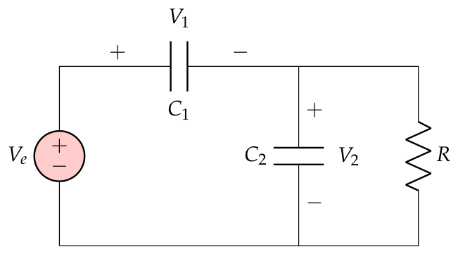
The first example is based on the electrical circuit depicted in Figure 1, introduced in [29] and used as a benchmark.

The dynamics are described by the following equations:

$$\left\{\begin{array}{c}{C}_1{\dot{V}}_1\left(t\right)=C_2{\dot{V}}_2\left(t\right)+{\displaystyle \frac{1}{R}}{V}_2\left(t\right)\hfill \\ 0=V_1\left(t\right)+V_2\left(t\right)+V_e\left(t\right)\hfill \end{array}\right..$$

(39)

where $V_1\left(t\right)$ and $V_2\left(t\right)$ denote the voltages across capacitors $C_1$ and $C_2$, respectively, while $V_e\left(t\right)$ is the input voltage. By introducing the state variables $x_1\left(t\right)=V_1\left(t\right)$ and $x_2\left(t\right)=V_2\left(t\right)$ and the input $u\left(t\right)=V_e\left(t\right)$, and adopting the circuit parameters $R=0.5$, $C_1=0.1$, and $C_2=0.5$ from [29], system (39) can be rewritten in the following singular system form:

$$\left\{\begin{array}{c}\mathbb{E}\dot{x}\left(t\right)=Ax\left(t\right)+\mathbb{B}u\left(t\right)+Fw\left(t\right)\hfill \\ y\left(t\right)=Cx\left(t\right)+\mathbb{D}u\left(t\right)+Hw\left(t\right)\hfill \end{array}\right.,$$

(40)

where

$$\begin{array}{cc}\hfill \mathbb{E}& =\left[\begin{array}{cc}0.1& -0.5\\ 0& 0\end{array}\right],A=\left[\begin{array}{cc}0& 2\\ 1& 1\end{array}\right],\mathbb{B}=\left[\begin{array}{c}0\\ 1\end{array}\right],\hfill \\ \hfill F& =\left[\begin{array}{c}1\\ 1\end{array}\right],C=\left[\begin{array}{cc}0& 1\end{array}\right],\mathbb{D}=0,H=0.1.\hfill \end{array}$$

(41)

With $Z={[0,1]}^T$,

Table 1. Minimum $H_{\infty }$ performance index ${\gamma }_{min}$ for the first example.

Method	${\mathit{\gamma }}_{min}$	Control K
Theorem 2 ($\alpha =1.6578,\beta =2.0409$)	$0.4000$	$\left[\begin{array}{cc}1.4422& -6.6731\end{array}\right]$
Theorem 2 ($\alpha =1,\beta =4.2913$)	$0.4853$	$\left[\begin{array}{cc}21.2767& -105.0576\end{array}\right]$
Theorem 3 $\left(30\right)$ in [16]	$0.5000$	—
Theorem 3 $\left(30\right)$–$\left(31\right)$ in [16]	$0.5000$	—

compares the minimum $H_{\infty }$ performance index ${\gamma }_{min}$ and the corresponding controller gain matrices obtained with the proposed approach and with the method in [16]. Two cases are considered: in the first case, ${\gamma }_{min}$ is optimized with respect to $\alpha$; in the second case, $\alpha =1$ to highlight the role of this scalar parameter. The results confirm the effectiveness of the proposed approach, which yields a smaller ${\gamma }_{min}$ and more favorable controller gains.

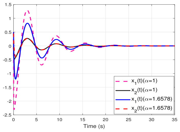
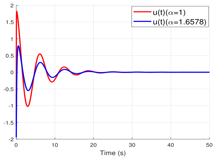
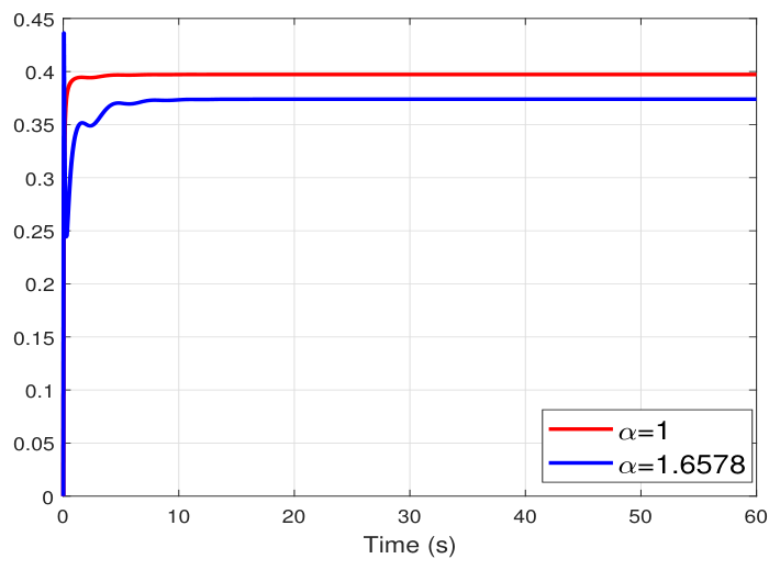
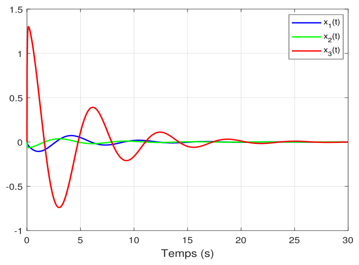
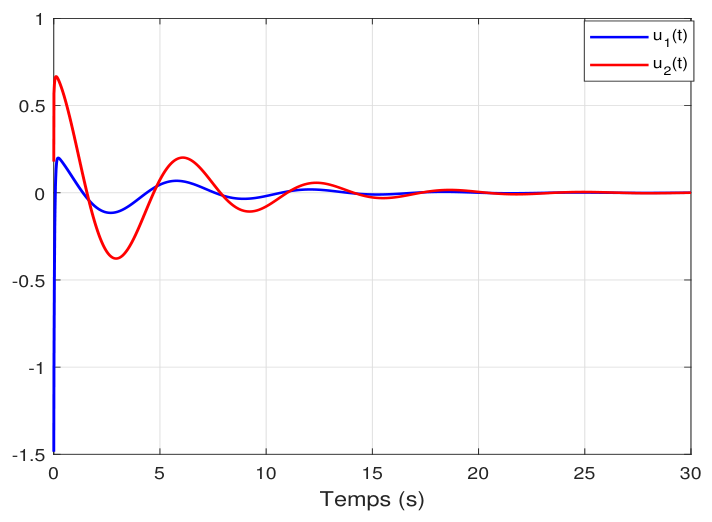
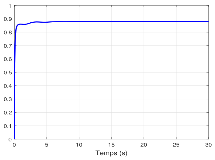
Simulation are performed to validate the designed controller for the two scenarios. The initial state is set to be $x\left(0\right)={\left[0.50.44736\right]}^T$ for $\alpha =1.6578$, and $x\left(0\right)={\left[0.50.11665\right]}^T$ for $\alpha =1$. The different initial conditions are due to the change in controller gain, which affects the consistent initial conditions: see [30,31,32,33]. The external disturbance is chosen in both cases to be $w\left(t\right)=e^{-0.2t}\cos \left(t\right)$. The simulation results are obtained by applying the controller gain matrices reported in Table 1 to system (41). Figure 2 shows the resulting state trajectories, which clearly converge to zero, while the corresponding control inputs $u\left(t\right)$ are presented in Figure 3. Furthermore, Figure 4 illustrates the evolution of the ratio $\sqrt{{\int }_0^{\infty }{y}^T\left(t\right)y\left(t\right)dt/{\int }_0^{\infty }{w}^T\left(t\right)w\left(t\right)dt}<\gamma$. The maximum value of this ratio is $0.3747$ for $\alpha =1.6578$ and $0.3972$ for $\alpha =1$, with both remaining significantly below the corresponding optimal performance index ${\gamma }_{min}$. These findings indicate that optimizing the proposed approach with respect to $\alpha$ reduces state magnitudes, control effort, and the $H_{\infty }$ performance ratio, confirming the effectiveness of the proposed design method.

5.2. Second Example

The following example adapted from [15] is now studied, with the following parameters:

$$\begin{array}{c}\hfill \mathbb{E}=\left[\begin{array}{ccc}1& 0& 0\\ 0& 1& 0\\ 0& 0& 0\end{array}\right],A=\left[\begin{array}{ccc}0& 1& 1\\ -1& 3& 0\\ 0& 0& 0\end{array}\right],\mathbb{B}=\left[\begin{array}{cc}0.1& -1.5\\ 1& 0.5\\ -0.1& 1\end{array}\right],\mathbb{F}=\left[\begin{array}{c}0\\ 1\\ -1\end{array}\right],\mathbb{M}=\left[\begin{array}{c}0.011\\ 0.12\end{array}\right],\\ \hfill J=\left[\begin{array}{ccc}1.5& 0& 2\\ -0.1& 2& 0\end{array}\right],C=\left[\begin{array}{ccc}1& 0& 1\\ -0.5& 1& 0\end{array}\right],\mathbb{D}=\left[\begin{array}{cc}0.32& -0.1\\ 0.13& 0.24\end{array}\right],\mathbb{H}=\left[\begin{array}{c}0.1\\ 0.02\end{array}\right].\end{array}$$

(42)

Choosing $\widehat{Z}={\left[\begin{array}{ccc}0& 0& 1\\ 0& 0& 1\end{array}\right]}^T$, the proposed condition in Theorem 3 is feasible, so it is possible to find a static output-feedback controller (30) with the $H_{\infty }$ performance $\gamma$ by solving the LMIs. Using the Matlab toolbox [28] to solve Theorem 3 with the optimized values of $\alpha =0.1113$ and $\beta =13.8344$, the minimum $H_{\infty }$ performance obtained is ${\gamma }_{min}=2.2072$, with the $H_{\infty }$ controller gain matrix

$$\mathbb{K}=\left[\begin{array}{cc}0.0049& -11.8510\\ 0.2825& 1.2497\end{array}\right].$$

(43)

The system described in (42) was simulated from zero initial conditions, with the disturbance taken as $w\left(t\right)=0.4e^{-0.32t}\sin \left(2t\right)$. The resulting trajectories of $x\left(t\right)$ and $u\left(t\right)$ are illustrated in Figure 5 and Figure 6, respectively. Figure 7 depicts the behavior of the ratio $\sqrt{{\int }_0^{\infty }{y}^T\left(t\right)y\left(t\right)dt/{\int }_0^{\infty }{w}^T\left(t\right)w\left(t\right)dt}<\gamma$. It is clear from Figure 7 that the ratio stays well below the prescribed value of $2.2072$, thereby validating the effectiveness of the condition established in Theorem 3.

To illustrate the advantage of the proposed method, the minimum performance index ${\gamma }_{min}$ obtained from Corollary 1 is considered. By using the same numerical example 2 in [15], the value of ${\gamma }_{min}$ obtained from Corollary 1 is $2.4215$, corresponding to the optimized values $\alpha =0.0156$ and $\beta =39.9975$. This value is significantly lower than the value $4.5$ reported in [15], thereby highlighting the superiority of the proposed approach. Moreover, to further highlight the benefit of introducing the scalar $\alpha$,

Table 2. Minimum $H_{\infty }$ performance index ${\gamma }_{min}$ for the second example.

Corollary 1 ($\mathit{\alpha }=0.0156,\mathit{\beta }=39.9975$)	Corollary 1 ($\mathit{\alpha }=1,\mathit{\beta }=35.0527$)	Corollary 1 in [15]
2.4215	6.6267	4.5

reports the results of Corollary 1 for two cases: one where ${\gamma }_{min}$ is optimized with respect to $\alpha$, and another where $\alpha =1$ is fixed. The comparison shows that incorporating $\alpha$ effectively reduces conservatism and yields a lower achievable ${\mathcal{H}}_{\infty }$ performance level.

6. Conclusions

This article has solved some problems in the control of continuous-time singular systems. More precisely, the $H_{\infty }$ state-feedback and the $H_{\infty }$ output-feedback control problems have been solved for these systems. The solution is based on mathematically combining a Lyapunov function approach with linear matrix inequality (LMI) techniques. Based on this, conditions were derived that guarantee admissibility and a prescribed $H_{\infty }$ performance level. A key feature of the proposed formulation is the generation of a parameterized family of LMIs, that makes possible the enlargement of the feasible solution set. The effectiveness of the proposed parameter in enlarging the feasible solution set relies on the existence of an admissible interval of $\alpha$ for which the resulting inequalities remain feasible. It is pointed out that due to the nonlinear interaction between the linear $\alpha {\tilde{Y}}_1$ and the quadratic term $-{\alpha }^2{\tilde{Y}}_2$, inappropriate choices may deteriorate the LMI condition. This will be the subject of future research. It is pointed out that the proposed formulation includes previous results in the literature as a special case when the parameter $\alpha$ is fixed to be $\alpha =1$. The simulation results demonstrate that the proposed conditions can achieve less conservative results than these methods in the literature. Future work will focus on extending the proposed framework to related classes of systems, in particular switched singular systems, singular systems with uncertainties, singular systems with time delays, and higher-index singular systems.

References

1. Dai, L. Singular Control Systems; Springer: Berlin/Heidelberg, Germany, 1989. [Google Scholar]
2. Xu, S.; Lam, J. Robust Control and Filtering of Singular Systems; Springer: Berlin/Heidelberg, Germany, 2006; Volume 332. [Google Scholar]
3. Ge, C.; Shi, Y.; Park, J.H.; Hua, C. Robust H stabilization for TS fuzzy systems with time-varying delays and memory sampled-data control. Appl. Math. Comput. 2019, 346, 500–512. [Google Scholar]
4. Li, M.; Sun, L.; Yang, R. Finite-time H control for a class of discrete-time nonlinear singular systems. J. Frankl. Inst. 2018, 355, 5384–5393. [Google Scholar] [CrossRef]
5. Zhang, Y.; Shi, P.; Nguang, S.K. Observer-based finite-time H control for discrete singular stochastic systems. Appl. Math. Lett. 2014, 38, 115–121. [Google Scholar] [CrossRef]
6. Feng, Z.; Shi, P. Two equivalent sets: Application to singular systems. Automatica 2017, 77, 198–205. [Google Scholar] [CrossRef]
7. Ji, X.; Su, H.; Chu, J. Robust state feedback H control for uncertain linear discrete singular systems. IET Control Theory Appl. 2007, 1, 195–200. [Google Scholar] [CrossRef]
8. Zhang, G.; Xia, Y.; Shi, P. New bounded real lemma for discrete-time singular systems. Automatica 2008, 44, 886–890. [Google Scholar] [CrossRef]
9. Zames, G. Feedback and optimal sensitivity: Model reference transformations, multiplicative seminorms, and approximate inverses. IEEE Trans. Autom. Control 1981, 26, 301–320. [Google Scholar] [CrossRef]
10. Song, B.; Zhang, Y.; Park, J.H. H control for Poisson-driven stochastic systems. Appl. Math. Comput. 2021, 392, 125716. [Google Scholar] [CrossRef]
11. Chadli, M.; Darouach, M. Novel bounded real lemma for discrete-time descriptor systems: Application to H control design. Automatica 2012, 48, 449–453. [Google Scholar] [CrossRef]
12. Feng, Y.; Yagoubi, M. On state feedback H control for discrete-time singular systems. IEEE Trans. Autom. Control 2013, 58, 2674–2679. [Google Scholar] [CrossRef]
13. Chang, X.H.; Wang, X.Y.; Hou, L.W. New LMI approach to H control of discrete-time singular systems. Appl. Math. Comput. 2024, 474, 128703. [Google Scholar] [CrossRef]
14. Delmotte, F.; Guerra, T.M.; Ksantini, M. Continuous Takagi–Sugeno’s models: Reduction of the number of LMI conditions in various fuzzy control design technics. IEEE Trans. Fuzzy Syst. 2007, 15, 426–438. [Google Scholar] [CrossRef]
15. Chadli, M.; Shi, P.; Feng, Z.; Lam, J. New bounded real lemma formulation and control for continuous-time descriptor systems. Asian J. Control 2017, 19, 2192–2198. [Google Scholar] [CrossRef]
16. Feng, Z.; Lam, J.; Xu, S.; Zhou, S. H control with transients for singular systems. Asian J. Control 2016, 18, 817–827. [Google Scholar] [CrossRef]
17. Chang, X.H.; Jin, X. Observer-based fuzzy feedback control for nonlinear systems subject to transmission signal quantization. Appl. Math. Comput. 2022, 414, 126657. [Google Scholar] [CrossRef]
18. Kamyar, R.; Peet, M.M.; Peet, Y. Solving large-scale robust stability problems by exploiting the parallel structure of Polya’s theorem. IEEE Trans. Autom. Control 2013, 58, 1931–1947. [Google Scholar] [CrossRef]
19. Benner, P.; Schneider, A. Model reduction for linear descriptor systems with many ports. In Progress in Industrial Mathematics at ECMI 2010; Springer: Berlin/Heidelberg, Germany, 2012; pp. 137–143. [Google Scholar]
20. Benson, S.J.; Ye, Y. DSDP5: Software For Semidefinite Programming; Technical Report ANL/MCS-P1289-0905; Mathematics and Computer Science Division, Argonne National Laboratory: Argonne, IL, USA, 2005. [Google Scholar]
21. Benson, S.J.; Ye, Y.; Zhang, X. Solving Large-Scale Sparse Semidefinite Programs for Combinatorial Optimization. SIAM J. Optim. 2000, 10, 443–461. [Google Scholar] [CrossRef]
22. Benson, S.J.; Ye, Y. Algorithm 875: DSDP5—Software for semidefinite programming. ACM Trans. Math. Softw. 2008, 34, 1–20. [Google Scholar] [CrossRef]
23. Stürz, Y.R.; Eichler, A.; Smith, R.S. Distributed control design for heterogeneous interconnected systems. IEEE Trans. Autom. Control 2020, 66, 5112–5127. [Google Scholar] [CrossRef]
24. Haiek Badreddine, E.; Aiss Hicham, E.; Abdelaziz, H.; Hajjaji Ahmed, E.; Houssaine Tissir, E. New approach to robust observer-based control of one-sided Lipschitz non-linear systems. IET Control Theory Appl. 2019, 13, 333–342. [Google Scholar] [CrossRef]
25. Zoulagh, T.; El Haiek, B.; Hmamed, A.; El Hajjaji, A. Homogenous polynomial H filtering for uncertain discrete-time systems: A descriptor approach. Int. J. Adapt. Control Signal Process. 2018, 32, 378–389. [Google Scholar] [CrossRef]
26. Zoulagh, T.; El Aiss, H.; Tadeo, F.; El Haiek, B.; Barbosa, K.A.; Hmamed, A. Gain-scheduled energy-to-peak approach for vehicle sideslip angle filtering. Symmetry 2024, 16, 1627. [Google Scholar] [CrossRef]
27. Badreddine, E.H.; Sadek, B.A.; Er-Rachid, I.; Barbosa, K.A. H Observer-Based Control for a Class of One-Sided Lipschitz Uncertain Systems in Finite Frequency Domain. Optim. Control Appl. Methods 2025, 46, 1708–1723. [Google Scholar] [CrossRef]
28. Gahinet, P.; Nemirovskii, A.; Laub, A.J.; Chilali, M. The LMI control toolbox. In Proceedings of the 1994 33rd IEEE Conference on Decision and Control; IEEE: Piscataway, NJ, USA, 1994; Volume 3, pp. 2038–2041. [Google Scholar]
29. Yang, Q.; Chang, X.H. Energy-to-peak controller design for discrete-time singular system. Circuits Syst. Signal Process. 2023, 42, 5944–5957. [Google Scholar] [CrossRef]
30. Campbell, S.L.; Meyer, C.D., Jr.; Rose, N.J. Applications of the Drazin inverse to linear systems of differential equations with singular constant coefficients. SIAM J. Appl. Math. 1976, 31, 411–425. [Google Scholar] [CrossRef]
31. Campbell, S.L. Singular Systems of Differential Equations II; Research Notes in Mathematics; Pitman Books Ltd.: London, UK; Pitman Publishing Inc.: Marshfield, MA, USA, 1982; Volume 40. [Google Scholar]
32. Owens, D.H.; Debeljkovic, D.L. Consistency and Liapunov stability of linear descriptor systems: A geometric analysis. IMA J. Math. Control Inf. 1985, 2, 139–151. [Google Scholar] [CrossRef]
33. Ezzine, F.; Hammami, M.A. Convergence and stability analysis of nonlinear singular systems: Application to circuit network. J. Nonlinear Math. Phys. 2024, 31, 69. [Google Scholar] [CrossRef]
Figure 1. Benchmark system for the first Example.
Symmetry 18 01014 g001
Figure 2. Responses of the system states x ( t ) for the first example.
Symmetry 18 01014 g002
Figure 3. Responses of the control input u ( t ) for the first example.
Symmetry 18 01014 g003
Figure 4. Evolution of the performance ratio 0 y T ( t ) y ( t ) d t / 0 w T ( t ) w ( t ) d t for the first example.
Symmetry 18 01014 g004
Figure 5. Responses of the system states x ( t ) for the second example.
Symmetry 18 01014 g005
Figure 6. Responses of the control input u ( t ) for the second example.
Symmetry 18 01014 g006
Figure 7. Evolution of the performance ratio 0 y T ( t ) y ( t ) d t / 0 w T ( t ) w ( t ) d t for the second example.
Symmetry 18 01014 g007