Approximate Analytical Solution of the Time-Fractional Sharma–Tasso–Olver Equations Under Singular and Non-Singular Kernel Operators

Abstract

The analysis of the time-fractional nonlinear Sharma–Tasso–Olver (STO) equation with various initial conditions has been shown in this work. Finding the appropriate approximate solution of the problems under consideration is carried out by implementing unique strategies that combine the Adomian decomposition method (ADM), and the Generalized integral transform. The proposed method computes the results as a convergent series. The main benefit of the suggested method is that it needs minimal computing effort while producing extremely accurate results. We first apply the fractional Caputo fractional derivative (CFD) and then the Atangana–Baleanu–Caputo (ABC) derivative to solve the fractional STO problem. The nonlinear wave model for harbor and coastal designs heavily relies on the wave solutions of the STO equation. Several cases of time-fractional STO equations with various initial approximations are used to illustrate the schemes under consideration. The efficiency and dependability of the methods under consideration are confirmed by executing suitable numerical simulations. We contrast our findings with those of other approaches, including the Homotopy perturbation method (HPM), and the q-Homotopy analysis Elzaki transform method (q-HAETM). Additionally, the results of using the proposed techniques at different fractional orders are analyzed, showing that their accuracy increases as the value goes from fractional order to integer order. The results gained indicate that the applied scheme is highly satisfying and investigate the complicated nonlinear problems that arise in innovation and science.

1. Introduction

Fractional calculus (FC) is a modern mathematical tool that is widely used in many branches of science and engineering. FC can be extended to a complex set and is characterised as a generalization of classical calculus in which we explore fractional-order differential and integral operators. The communication between Leibniz and L’Hospital is where the concept of fractional calculus was first developed. Many mathematicians have developed a number of fractional differential and integral operators in the last few decades, strengthening this idea [1,2]. The nonlocality of the fractional operators is used to perform the progressive functioning of the classical derivatives demonstration. It is evident that fractional operators specify complex memory and a variety of objects that can be examined with standard mathematical techniques like classical differential calculus. In recent years, nonlocal fractional operators without a unique kernel have been described and proposed. However, the application of the FC concept in different fields of study is still in its early stages. Recently, FC has become a very promising technique because of its wider applicability in complex nonlinear phenomenon dynamics. The basic theory and operator features shown in the framework of fractional calculus have been used by a number of researchers to investigate models of signal processing [3], chaos theory [4], continuum mechanics [5], optimal control problems [6], complex networks [7], and other areas [8,9,10]. In the past several years, more researchers began to employ this calculus to study a range of natural processes because scientists were previously unaware of its significance [11,12,13]. Furthermore, it was demonstrated that FC is far more appropriate than traditional calculus for handling the majority of challenging real-world problems. The richness of applied research in fractional calculus has increased throughout time. Numerous studies have demonstrated its ability to address a wide range of problems, especially in scientific disciplines such as image processing [14], robotics [15], viscoelasticity [16], and several others [17,18,19,20,21].

Fractional derivatives can be defined in a number of different ways, including Grünwald–Letnikov, Riemann–Liouville, Caputo, Caputo–Fabrizio (CF), and Atangana–Baleanu (AB) derivatives. Numerous scholars have not used the Riemann–Liouville fractional derivative extensively to solve real-world physical issues since it is incompatible with common initial conditions that are often seen in such situations. Caputo was able to solve numerous fractional-order physics problems by developing a new definition that may utilize the initial conditions to address this challenge [22]. The Caputo–Fabrizio (CF) fractional derivative is a definition that was recently proposed by Caputo and Fabrizio [23]. In comparison to earlier definitions, they demonstrated that the derivative is not based on a single kernel, allowing for more precise solutions to numerous fractional differential equations in a variety of areas [24,25,26]. Meanwhile, this concept has been criticized by certain authors in articles that deal with specific models that use a nonlocal and non-singular kernel. Atangana and Baleanu (AB) proposed a new definition of fractional differentiation that includes a non-singular and nonlocal kernel in order to overcome this restriction [27]. Based on the generalized Mittag-Leffler function, which functions as a non-singular and nonlocal kernel and satisfies the fundamental requirements of fractional derivatives, this formulation was known as the Atangana–Baleanu (AB) fractional derivative. Several mathematical models in various fields have benefited greatly from the application of this definition [28,29,30]. It has been shown that this formulation provides better precision and clarity than previous fractional derivatives, allowing for a more descriptive examination of solution properties.

Many different areas of physics and engineering have seen a growing interest in mathematical modeling in practical applications in recent years, which typically leads to nonlinear fractional partial and ordinary differential equations [31,32,33,34,35]. As a result, their numerous applications have recently generated a great deal of interest in them. In practical mathematics, it is crucial to find analytic numerical solutions for these fractional differential equations. Finding approximate solutions is important in science because there is generally no method that provides an exact solution for fractional differential equations. The literature has used a variety of methods to solve fractional-order PDEs, including the Yang transform iterative method [36], Laplace residual power series method [37], Homotopy perturbation transform method [38,39], Approximate analytical method [40], Homotopy analysis method [41], and many more [42,43,44,45,46]. An important aspect of studying the nonlinear field is the investigation of soliton solutions of complex nonlinear evolution equations. These answers provide valuable insights into the fundamentals of nonlinear science. The STO equation was developed by Olver. The equation originated from research on evolution equations with an infinite number of symmetries. It is frequently thought of as a generalization of the modified KdV, Burgers, and KdV equations. The following are the nonlinear time-fractional STO equations that we are examining in this article:

$$\begin{array}{c}\hfill \begin{array}{cc}& D_{\vartheta }^{\mathtt{p}}\mathtt{z}+\lambda {\left({\mathtt{z}}^3\right)}_{\chi }+{\displaystyle \frac{3}{2}}\lambda {\left({\mathtt{z}}^2\right)}_{\chi \chi }+\lambda {\left(\mathtt{z}\right)}_{\chi \chi \chi }=0,\hfill \end{array}\end{array}$$

(1)

with initial condition

$$\begin{array}{c}\hfill \mathtt{z}(\chi ,0)=\sqrt{{\displaystyle \frac{1}{\lambda }}}\tanh \left(\sqrt{{\displaystyle \frac{1}{\lambda }}}\chi \right),\end{array}$$

(2)

and

$$\begin{array}{c}\hfill \begin{array}{cc}& D_{\vartheta }^{\mathtt{p}}\mathtt{z}+3\lambda {\left({\mathtt{z}}^2\right)}_{\chi }+3\lambda {\mathtt{z}}^2{\left(\mathtt{z}\right)}_{\chi }+3\lambda \mathtt{z}{\left(\mathtt{z}\right)}_{\chi \chi }+\lambda {\left(\mathtt{z}\right)}_{\chi \chi \chi }=0,\hfill \end{array}\end{array}$$

(3)

with initial condition

$$\begin{array}{c}\hfill \mathtt{z}(\chi ,0)={\displaystyle \frac{2\sigma \left(\tanh \right(\sigma \chi )+\varpi )}{1+\varpi \tanh \left(\sigma \chi \right)}}.\end{array}$$

(4)

where $\lambda$ is constant. $\mathtt{z}$ is the dependent wave function and $\chi$ and $\vartheta$ are the temporal and spatial variables, respectively. Similar to the KdV equation, the STO equation can explain evolutionary physics occurrences and their interactions with nonlinear waves, such as fluid dynamics, continuum mechanics, turbulence and solitons, aerodynamics, etc. The linear dispersive term and the double nonlinear term are both included in the STO equation. The fusion and fission of the solitary wave solutions have been obtained by applying Hirota’s direct approach and the Backlund transformation. It has been found that waves with $\lambda <0$ represent the fission of solutions, while waves with $\lambda >0$ only show the fusion of solutions [47]. Several approaches have been used to obtain the solution to the STO equation, including the Laplace residual power series method [48], the new extended direct algebraic method [49], modified Homotopy analysis transform method [50], and many more. This work aims to enhance the Generalized transform decomposition method (GTDM) in order to provide an approximate solution of the STO in terms of CFD and ABC manner. The main goal is to investigate the differences between the classical Caputo derivative and the ABC derivative. In order to do this, we take into consideration two useful cases, each of which uses one of the two derivative definitions and is formulated under a single initial condition. The ABC derivative provides improved modeling capabilities for complex systems through its generalized, non-singular memory kernel, while the Caputo derivative is commonly used because it performs well with classical models and basic initial conditions.

The Generalized integral transform (GIT) [51], and the Adomian decomposition method (ADM) [52,53] are combined to create the suggested technique, which handles nonlinear and fractional differential equations without linearization or small-parameter assumptions. Compared to fixed-parameter transforms like Laplace, the Jafari transform offers greater control over convergence for stiff or unique problems since it has an adjustable parameter in the kernel. It unifies several transforms: although Laplace, Sumudu, and Elzaki are all special cases derived by particular selections of $\omega \left(s_1\right)$ and $g\left(\mathtt{s}\right)$, they can all be covered by a single approach. The technique expands the nonlinear terms using Adomian-type polynomials and transforms differential operators into algebraic form using a generic kernel. Compared to classical perturbation or standard decomposition methods, it improves accuracy and lowers computational effort by directly handling complex nonlinearity and memory effects through the transform–decomposition relationship.

Recent work shows that a GIT and ADM may solve nonlinear fractional PDEs with fewer terms and faster convergence than Laplace or Sumudu-based approaches. For complex and highly nonlinear problems, standard ADM frequently converges slowly or diverges because it only uses series decomposition. This is improved by Laplace–ADM and Sumudu–ADM, which use a fixed transform to translate differential operators into algebraic form, although they are restricted to the particular characteristics of one transform. By enabling the kernel to be selected or modified to fit the equation’s structure, GTDM eliminates this limitation and essentially preconditions the problem such that each term in the decomposition gets smaller more quickly. This improves accuracy with fewer terms, especially for memory-dependent and fractional equations where the transform’s ability to handle nonlocal operators is crucial. GTDM includes initial conditions of all orders directly requiring further assumptions, while ADM requires direct substitution, and q-HAM/q-HATM need an auxiliary linear operator to insert initial conditions. GTDM needs fewer terms in its series expansion to arrive nearly to the exact solution since it offers higher levels of precision with much fewer computational steps. In comparison to traditional ADM variations, which frequently struggle with complex computations when handling strongly nonlinear or fractional-order problems, this quick rate of convergence significantly decreases CPU time and computational memory utilization. Additionally, GTDM constantly generates significantly lower error margins within a wider domain, as shown by quantitative error analysis such as calculating the maximum absolute errors, root mean square errors, and relative error. This proves that GTDM is highly efficient and computationally superior to established methods.

When compared to classical decomposition or Laplace transform approaches, the employment of the GIT with the Adomian method is a new addition that improves convergence and lowers computing cost. Additionally, a strong convergence and error analysis are presented, providing theoretical support not seen in earlier studies. Our method provides the solution in series form for the numerical cases. When considered in closed form, the series provides precise solutions to the basic equations. Scholars can use this work as a central reference to investigate this method and use it in a variety of applications to obtain approximate results in a few easy steps. The unique feature of this effort is the depiction of an innovative method for solving STO with minimal and consecutive steps. The representation of the novel approach to solving STO with few and sequential stages is what makes this endeavor special. The remainder of this work is structured as follows: We provide some key information and definitions pertaining to fractional calculus in Section 2. Section 3 introduces the GTDM. We present the existence result of the suggested methods in Section 4. Section 5 focuses on using the technique to test problems and presents graphs demonstrating the efficacy of the suggested approach for specific values of $\chi$ and $\vartheta$. The achieved results are discussed in detail in Section 6. Lastly, the paper’s conclusion is given in Section 7.

2. Preliminaries

In this part, we offer few definitions of fractional operators related to our work.

Definition 1. 

The CFD is as [54]:

$$\begin{array}{c}\hfill {}_0{}^c\mathbf{D}_{\vartheta }^{\mathcal{p}}\left(\mathcal{z}\left(\vartheta \right)\right)=\left\{\begin{array}{c}{\displaystyle \frac{1}{\mathsf{\Gamma }(r-\mathcal{p})}}{\displaystyle \frac{d}{d{\vartheta }^r}}{\displaystyle \underset{0}{\overset{\vartheta }{\int }}}{\displaystyle \frac{\mathcal{z}\left(\vartheta \right)}{{(\vartheta -\psi )}^{\mathcal{p}+1-r}}}d\psi ,r-1<\mathcal{p}<r,\hfill \\ {\displaystyle \frac{d^r}{d{\vartheta }^r}}\mathcal{z}\left(\vartheta \right),\mathcal{p}=r.\hfill \end{array}\right.\end{array}$$

(5)

Definition 2. 

The ABC operator is as [27]:

$$\begin{array}{c}\hfill {}_{{\eta }_1 }{}^{ABC}\mathbf{D}_{\vartheta }^{\mathcal{p}}\left(\mathcal{z}\left(\vartheta \right)\right)={\displaystyle \frac{\mathbb{U}\left(\mathcal{p}\right)}{1-\mathcal{p}}}{\displaystyle \underset{0}{\overset{\vartheta }{\int }}}{\mathcal{z}}^{\prime }\left(\chi \right)E_{\mathcal{p}}\left[-{\displaystyle \frac{\mathcal{p}{(\vartheta -\chi )}^{\mathcal{p}}}{1-\mathcal{p}}}\right]d\chi ,\vartheta >0,\end{array}$$

(6)

where $\mathcal{z}\in {\mathcal{H}}^1(a_1,a_2)\left(Sobolevspace\right),a_1<a_2,\mathcal{p}\in [0,1]$, $E_{\mathcal{p}}$ is the Mittag-Leffler function and $\mathbb{U}\left(\mathcal{p}\right)$ demonstrates a normalization function as $\mathbb{U}\left(\mathcal{p}\right)=\mathbb{U}\left(0\right)=\mathbb{U}\left(1\right)=1.$

Definition 3. 

The $ABC$ integral operator is as [27]:

$$\begin{array}{c}\hfill {}_{{\eta }_1 }{}^{ABC}\mathcal{I}_{\vartheta }^{\mathcal{p}}\left(\mathcal{z}\left(\vartheta \right)\right)={\displaystyle \frac{1-\mathcal{p}}{\mathbb{U}\left(\mathcal{p}\right)}}\mathcal{z}\left(\vartheta \right)+{\displaystyle \frac{\mathcal{p}}{\mathsf{\Gamma }\left(\mathcal{p}\right)\mathbb{U}\left(\mathcal{p}\right)}}{\displaystyle \underset{{\eta }_1}{\overset{\vartheta }{\int }}}\mathcal{z}\left(\chi \right){(\vartheta -\chi )}^{\mathcal{p}-1}d\chi .\end{array}$$

(7)

Definition 4. 

Taking an integrable mapping $\mathcal{z}\left(\vartheta \right)$ on a set $\mathcal{P},$ so [51]

$$\begin{array}{c}\hfill \mathcal{P}=\left\{\mathcal{z}\left(\vartheta \right):\exists M>0,\kappa >0,\left|\mathcal{z}\right(\vartheta \left)\right|<M\exp \left(\kappa \vartheta \right),if\vartheta \ge 0\right\}.\end{array}$$

(8)

Definition 5. 

Assume the mappings $\omega \left(\mathcal{s}\right),g\left(\mathcal{s}\right):{\mathbb{R}}^{+}\mapsto {\mathbb{R}}^{+}$ with $\phi \left(\mathcal{s}\right)\ne 0\forall \mathcal{s}\in {\mathbb{R}}^{+}.$ The GIT of the mapping $\mathcal{z}\left(\vartheta \right)$ indicated by $\mathbf{Q}\left(\mathcal{s}\right)$ as [51]

$$\begin{array}{c}\hfill \mathit{J}\left\{\mathcal{z}\left(\vartheta \right),\mathcal{s}\right\}=\mathbf{Q}\left(\mathcal{s}\right)=\omega \left(s_1\right){\displaystyle \underset{0}{\overset{\infty }{\int }}}\mathcal{z}\left(\vartheta \right)\exp (-g\left(\mathcal{s}\right)\vartheta )d\vartheta .\end{array}$$

(9)

Theorem 1. 

Convolution property: For GIT, the subsequent holds true [51]:

$$\begin{array}{c}\hfill \mathit{J}\left\{{\mathcal{z}}_1\ast {\mathcal{z}}_2\right\}={\displaystyle \frac{1}{\omega \left(\mathcal{s}\right)}}{\mathbf{Q}}_1\left(\mathcal{s}\right)\ast {\mathbf{Q}}_2\left(\mathcal{s}\right).\end{array}$$

(10)

Definition 6. 

The GIT of the CFD is as:

$$\begin{array}{c}\hfill \mathit{J}\left\{{}_0{}^c\mathbf{D}_{\vartheta }^{\mathcal{p}}\left(\mathcal{z}\left(\vartheta \right)\right),\mathcal{s}\right\}={\mathrm{g}}^{\mathcal{p}}\left(\mathcal{s}\right)\mathbf{Q}\left(s_1\right)-\omega \left(\mathcal{s}\right){\displaystyle \sum _{\kappa =0}^{\mathcal{p}-1}}{\mathrm{g}}^{\mathcal{p}-\kappa -1}\left(s_1\right){\mathcal{z}}^{\left(\kappa \right)}\left(0\right),r-1<\mathcal{p}<r,\omega ,\mathrm{g}>0.\end{array}$$

(11)

Remark 1. 

Definition 6 offers the outcomes given below:

1.  Inserting $\omega \left(\mathcal{s}\right)=1$ and g$\left(\mathcal{s}\right)=\mathcal{s},$ thus, we acquire the Laplace transform [55].

2.  Inserting $\omega \left(\mathcal{s}\right){\displaystyle \frac{1}{\mathcal{s}}}$ and g$\left(\mathcal{s}\right)={\displaystyle \frac{1}{\mathcal{s}}},$ thus, we acquire the $\mathcal{p}$-Laplace transform [56].

3.  Inserting $\omega \left(\mathcal{s}\right)={\displaystyle \frac{1}{\mathcal{s}}}$ and g$\left(\mathcal{s}\right)={\displaystyle \frac{1}{\mathcal{s}}},$ thus, we acquire the Sumudu transform [57].

4.  Inserting $\omega \left(\mathcal{s}\right)={\displaystyle \frac{1}{\mathcal{s}}}$ and g$\left(\mathcal{s}\right)=1,$ thus, we acquire the Aboodh transform [58].

5.  Inserting $\omega \left(\mathcal{s}\right)=\mathcal{s}$ and g$\left(\mathcal{s}\right)={\mathcal{s}}^2,$ thus, we acquire the Pourreza transform [59,60].

6.  Inserting $\omega \left(\mathcal{s}\right)=\mathcal{s}$ and g$\left(\mathcal{s}\right)={\displaystyle \frac{1}{\mathcal{s}}},$ thus, we acquire the Elzaki transform [61].

7.  Inserting $\omega \left(\mathcal{s}\right)={\mathbf{w}}_2$ and g$\left(\mathcal{s}\right)={\displaystyle \frac{\mathcal{s}}{{\mathbf{w}}_2}},$ thus, we acquire the Natural transform [62].

8.  Inserting $\omega \left(\mathcal{s}\right)={\mathcal{s}}^2$ and g$\left(\mathcal{s}\right)=\mathcal{s},$ thus, we acquire the Mohand transform [63].

9.  Inserting $\omega \left(\mathcal{s}\right)={\displaystyle \frac{1}{{\mathcal{s}}^2}}$ and g$\left(\mathcal{s}\right)={\displaystyle \frac{1}{\mathcal{s}}},$ thus, we acquire the Swai transform [64].

10.  Inserting $\omega \left(\mathcal{s}\right)=1$ and g$\left(\mathcal{s}\right)={\displaystyle \frac{1}{\mathcal{s}}},$ thus, we acquire the Kamal transform [65].

11. Inserting $\omega \left(\mathcal{s}\right)={\mathcal{s}}^{\mathcal{p}}$ and g$\left(\mathcal{s}\right)={\displaystyle \frac{1}{\mathcal{s}}},$ thus, we acquire the G−transform [66,67].

Definition 7. 

The GIT of the $ABC$ derivative is as [68]:

$$\begin{array}{c}\hfill \mathit{J}{\{}_0^{ABC}{\mathbf{D}}_{\vartheta }^{\mathcal{p}}\left(\mathcal{z}\left(\vartheta \right)\right),\mathcal{s}\}\left(\mathcal{p}\right)={\displaystyle \frac{\mathbb{U}\left(\mathcal{p}\right){\mathrm{g}}^{\mathcal{p}}\left(\mathcal{s}\right)}{\mathcal{p}+(1-\mathcal{p}){\mathrm{g}}^{\mathcal{p}}\left(\mathcal{s}\right)}}\left(\mathbf{Q}\left(\mathcal{s}\right)-{\displaystyle \frac{\omega \left(\mathcal{s}\right)}{\mathrm{g}\left(\mathcal{s}\right)}}\mathcal{z}\left(0\right)\right).\end{array}$$

(12)

Remark 2. 

Definition 7 leads to the below consequences:

1.  Inserting $\omega \left(\mathcal{s}\right)=1$ and $\mathrm{g}\left(\mathcal{s}\right)=\mathcal{s},$ thus, we acquire the Laplace transform of fractional ABC operator [69].

2.  Inserting $\omega \left(\mathcal{s}\right)=\mathcal{s}$ and $\mathrm{g}\left(\mathcal{s}\right)={\displaystyle \frac{1}{\mathcal{s}}},$ thus, we acquire the Elzaki transform of fractional ABC operator [70].

3.  Inserting $\omega \left(\mathcal{s}\right)=\mathrm{g}\left(\mathcal{s}\right)={\displaystyle \frac{1}{\mathcal{s}}},$ thus, we acquire the Sumudu transform of fractional ABC operator [71].

4.  Inserting $\omega \left(\mathcal{s}\right)=1$ and $\mathrm{g}\left(\mathcal{s}\right)=\mathcal{s}/{\mathbf{w}}_2,$ thus, we acquire the Shehu transform of fractional ABC operator [71].

Definition 8. 

The Mittag-Leffler function is as [72]

$$\begin{array}{c}\hfill E_{\mathcal{p}}\left(z\right)={\displaystyle \sum _{\kappa =0}^{\infty }}{\displaystyle \frac{z_1^{\kappa }}{\mathsf{\Gamma }(\kappa \mathcal{p}+1)}},\mathcal{p},z_1\in \mathbb{C},\Re \left(\mathcal{p}\right)\ge 0.\end{array}$$

(13)

3. Procedure of the GTDM

Assuming the fractional PDE as given below:

$$\begin{array}{c}\hfill {\mathbf{D}}_{\vartheta }^{\mathtt{p}}\mathtt{z}(\chi ,\vartheta )+\pounds \mathtt{z}(\chi ,\vartheta )+\mathcal{U}\mathtt{z}(\chi ,\vartheta )=\mathcal{F}(\chi ,\vartheta ),\vartheta >0,0<\mathtt{p}\le 1,\end{array}$$

(14)

with

$$\begin{array}{c}\hfill \mathtt{z}(\chi ,0)=\mathcal{J}\left(\chi \right),\end{array}$$

(15)

here ${\mathbf{D}}_{\vartheta }^{\mathtt{p}}={\displaystyle \frac{{\partial }^{\mathtt{p}}\mathtt{z}(\chi ,\vartheta )}{\partial {\vartheta }^{\mathtt{p}}}}$ specifies the derivative having $\mathtt{p}\in (0,1]$ whereas £ and $\mathcal{U}$ demonstrate the linear and nonlinear terms. In addition, $\mathtt{F}(\chi ,\vartheta )$ indicates the source term.

Inserting GIT to (14), we achieve

$$\begin{array}{c}\hfill \mathit{J}\left[{\mathbf{D}}_{\vartheta }^{\mathtt{p}}\mathtt{z}(\chi ,\vartheta )+\pounds \mathtt{z}(\chi ,\vartheta )+\mathcal{U}\mathtt{z}(\chi ,\vartheta )\right]=\mathit{J}\left[\mathcal{F}(\chi ,\vartheta )\right].\end{array}$$

The GIT is first implemented using a CFD operator. Next, we use the ABC derivative as follows:

$$\begin{array}{c}{g}^{\mathtt{p}}\left(\mathtt{s}\right)\mathcal{V}(\chi ,\mathtt{s})=\omega \left(\mathtt{s}\right){\displaystyle \sum _{\kappa =0}^{\mu -1}}{g}^{\mathtt{p}-1-\kappa }\left(\mathtt{s}\right){\mathtt{z}}^{\left(\kappa \right)}\left(0\right)+\mathit{J}\left[\pounds \mathtt{z}(\chi ,\vartheta )+\mathcal{U}\mathtt{z}(\chi ,\vartheta )\right]+\mathit{J}\left[\mathcal{F}(\chi ,\vartheta )\right],\hfill \end{array}$$

(16)

and

$$\begin{array}{c}{\displaystyle \frac{g^{\mathtt{p}}\left(\mathtt{s}\right)\mathbb{U}\left(\mathtt{p}\right)}{\mathtt{p}+(1-\mathtt{p})g^{\mathtt{p}}\left(\mathtt{s}\right)}}\mathcal{V}(\chi ,\mathtt{s})={\displaystyle \frac{\omega \left(\mathtt{s}\right)}{g\left(\mathtt{s}\right)}}{\displaystyle \frac{g^{\mathtt{p}}\left(\mathtt{s}\right)\mathbb{U}\left(\mathtt{p}\right)}{\mathtt{p}+(1-\mathtt{p})g^{\mathtt{p}}\left(\mathtt{s}\right)}}\mathtt{z}\left(0\right)+\mathit{J}\left[\pounds \mathtt{z}(\chi ,\vartheta )+\mathcal{U}\mathtt{z}(\chi ,\vartheta )\right]+\mathit{J}\left[\mathcal{F}(\chi ,\vartheta )\right].\hfill \end{array}$$

(17)

The inverse GIT of (16) and (17) offers

$$\begin{array}{c}\hfill \mathtt{z}(\chi ,\vartheta )={\mathit{J}}^{-1}\left[\omega \left(\mathtt{s}\right){\displaystyle \sum _{\kappa =0}^{\mu -1}}g{\left(\mathtt{s}\right)}^{\mathtt{p}-\kappa -1}{\mathtt{z}}^{\left(\kappa \right)}\left(0\right)+{\displaystyle \frac{1}{g^{\mathtt{p}}\left(\mathtt{s}\right)}}\mathit{J}\left[\mathcal{F}(\chi ,\vartheta )\right]\right]-{\mathit{J}}^{-1}\left[{\displaystyle \frac{1}{g^{\mathtt{p}}\left(\mathtt{s}\right)}}\mathit{J}\left[\pounds \mathtt{z}(\chi ,\vartheta )+\mathcal{U}\mathtt{z}(\chi ,\vartheta )\right]\right],\end{array}$$

(18)

and

$$\begin{array}{c}\hfill \mathtt{z}(\chi ,\vartheta )={\mathit{J}}^{-1}\left[{\displaystyle \frac{\omega \left(\mathtt{s}\right)}{g\left(\mathtt{s}\right)}}\mathtt{z}\left(0\right)+{\displaystyle \frac{\mathtt{p}+(1-\mathtt{p})g^{\mathtt{p}}\left(\mathtt{s}\right)}{g^{\mathtt{p}}\left(\mathtt{s}\right)\mathbb{U}\left(\mathtt{p}\right)}}\mathit{J}\left[\mathcal{F}(\chi ,\vartheta )\right]\right]-{\mathit{J}}^{-1}\left[{\displaystyle \frac{\mathtt{p}+(1-\mathtt{p})g^{\mathtt{p}}\left(\mathtt{s}\right)}{g^{\mathtt{p}}\left(\mathtt{s}\right)\mathbb{U}\left(\mathtt{p}\right)}}\mathit{J}\left[\pounds \mathtt{z}(\chi ,\vartheta )+\mathcal{U}\mathtt{z}(\chi ,\vartheta )\right]\right].\end{array}$$

(19)

The GTDM series form solution of $\mathtt{z}(\chi ,\vartheta )$ is as

$$\begin{array}{c}\hfill \mathtt{z}(\chi ,\vartheta )={\displaystyle \sum _{\mu =0}^{\infty }}{\mathtt{z}}_{\mu }(\chi ,\vartheta ).\end{array}$$

(20)

Additionally, the nonlinear term $\mathcal{U}(\chi ,\vartheta )$ is specified as

$$\begin{array}{c}\hfill \mathcal{U}\mathtt{z}(\chi ,\vartheta )={\displaystyle \sum _{\mu =0}^{\infty }}{\tilde{A}}_{\mu }({\mathtt{z}}_0,{\mathtt{z}}_1,...),\mu =0,1,\dots ,\end{array}$$

(21)

where

$${\tilde{A}}_{\mu }({\mathtt{z}}_0,{\mathtt{z}}_1,\dots )={\displaystyle \frac{1}{\mu !}}{\left[{\displaystyle \frac{d^{\mu }}{d{\mathtt{p}}^{\mu }}}\mathcal{U}\left({\displaystyle \sum _{j=0}^{\infty }}{\mathtt{p}}^j{\mathtt{z}}_j\right)\right]}_{\mathtt{p}=0},\mu >0.$$

Inserting (20) and (21) into (18) and (19), respectively, we achieve

$$\begin{array}{ccc}\hfill {\displaystyle \sum _{\mu =0}^{\infty }}{\mathtt{z}}_{\mu }(\chi ,\vartheta )& & =\mathcal{J}\left(\chi \right)+\tilde{\mathcal{J}}\left(\chi \right)-{\mathit{J}}^{-1}\left[{\displaystyle \frac{1}{g^{\mathtt{p}}\left(\mathtt{s}\right)}}\mathit{J}[\pounds \mathtt{z}(\chi ,\vartheta )+{\displaystyle \sum _{\mu =0}^{\infty }}{\tilde{A}}_{\mu }]\right],\hfill \end{array}$$

(22)

and

$$\begin{array}{ccc}\hfill {\displaystyle \sum _{\mu =0}^{\infty }}{\mathtt{z}}_{\mu }(\chi ,\vartheta )& & =\mathcal{J}\left(\chi \right)+\tilde{\mathcal{J}}\left(\chi \right)-{\mathit{J}}^{-1}\left[{\displaystyle \frac{\mathtt{p}+(1-\mathtt{p})g^{\mathtt{p}}\left(\mathtt{s}\right)}{\mathbb{U}\left(\mathtt{p}\right)g^{\mathtt{p}}\left(\mathtt{s}\right)}}\mathit{J}[\pounds \mathtt{z}(\chi ,\vartheta )+{\displaystyle \sum _{\mu =0}^{\infty }}{\tilde{A}}_{\mu }]\right].\hfill \end{array}$$

(23)

So, the achieved result for (22) and (23) is indicated as:

$$\begin{array}{ccc}\hfill {\mathtt{z}}_0(\chi ,\vartheta )& & =\mathcal{J}\left(\chi \right)+\tilde{\mathcal{J}}\left(\chi \right),\mu =0,\hfill \\ \hfill {\mathtt{z}}_{\mu +1}(\chi ,\vartheta )& & =-{\mathit{J}}^{-1}\left[{\displaystyle \frac{1}{g^{\mathtt{p}}\left(\mathtt{s}\right)}}\mathit{J}[\pounds \left({\mathtt{z}}_{\mu }(\chi ,\vartheta )\right)+{\displaystyle \sum _{\mu =0}^{\infty }}{\tilde{A}}_{\mu }]\right],\mu \ge 1,\hfill \\ \hfill {\mathtt{z}}_{\mu +1}(\chi ,\vartheta )& & =-{\mathit{J}}^{-1}\left[{\displaystyle \frac{\mathtt{p}+(1-\mathtt{p})g^{\mathtt{p}}\left(\mathtt{s}\right)}{\mathbb{U}\left(\mathtt{p}\right)g^{\mathtt{p}}\left(\mathtt{s}\right)}}\mathit{J}[\pounds \left({\mathtt{z}}_{\mu }(\chi ,\vartheta )\right)+{\displaystyle \sum _{\mu =0}^{\infty }}{\tilde{A}}_{\mu }]\right],\mu \ge 1.\hfill \end{array}$$

(24)

4. Convergence Analysis of the GTDM

This part explains how the presence of suitable specifications guarantees the development of a unique solution. Regarding GDM, the existence of our proposed solutions is demonstrated by [73].

Theorem 2. 

(Uniqueness theorem): Equation (24) has a unique solution if $0<{\displaystyle \frac{\left({\varsigma }_1+{\varsigma }_2\right){\vartheta }^{\left(\mathcal{p}\right)}}{\mathsf{\Gamma }(\mathcal{p}+1)}}<1,$ for some positive constants ${\varsigma }_1,{\varsigma }_2.$

Proof. 

Suppose $\mathsf{\Pi }=\left(\mathbb{C}\right([0,T],\parallel .\parallel )$ is Banach space ∀ continuous function on $[0,T]$ having norm $\left|\right|\mathtt{z}(\chi ,\vartheta )\left|\right|={max}_{\vartheta \in \mathtt{I}}\left|\mathtt{z}(\chi ,\vartheta )\right|$. Let $\mathcal{V}:\mathsf{\Pi }\mapsto \mathsf{\Pi }$ is a nonlinear mapping, so

$$\begin{array}{c}\hfill {\mathtt{z}}_{\mu +1}(\chi ,\vartheta )={\mathtt{z}}_0(\chi ,\vartheta )+{\mathit{J}}^{-1}\left[{\displaystyle \frac{1}{g^{\mathtt{p}}\left(\mathtt{s}\right)}}\mathit{J}\left[\pounds \left[{\mathtt{z}}_{\mu }(\chi ,\vartheta )\right]+\mathcal{U}\left[{\mathtt{z}}_{\mu }(\chi ,\vartheta )\right]\right]\right],\mu \ge 0,\end{array}$$

(25)

Consider that $\pounds \left[\mathtt{z}(\chi ,\vartheta )\right]$ and $\mathcal{U}\left[\mathtt{z}(\chi ,\vartheta )\right]$ are also Lipschitzian with $|\pounds \mathtt{z}-\pounds \widehat{\mathtt{z}}|<{\varsigma }_1|\mathtt{z}-\widehat{\mathtt{z}}|$ and $|\mathcal{U}\mathtt{z}-\mathcal{U}\widehat{\mathtt{z}}|<{\varsigma }_2|\mathtt{z}-\widehat{\mathtt{z}}|$, where ${\varsigma }_1$ and ${\varsigma }_2$ are Lipschitz constants respectively and $\mathtt{z},\widehat{\mathtt{z}}$ are two different functional values.

For all $\mathtt{z}(\chi ,\vartheta ),\mathtt{z}(\chi ,\vartheta )\in \mathbb{C}\left(\right[0,T\left]\right)$ and $\vartheta \in [0,T]$, we may have

$$\parallel \mathcal{V}\mathtt{z}-\mathcal{V}\widehat{\mathtt{z}}\parallel =\underset{\vartheta \in \mathcal{I}}{\max }\left|\begin{array}{cc}& {\mathit{J}}^{-1}\left[{\displaystyle \frac{1}{g^{\mathtt{p}}\left(\mathtt{s}\right)}}\mathit{J}\left[\pounds \left[\mathtt{z}(\chi ,\vartheta )\right]+\mathcal{U}\left[\mathtt{z}(\chi ,\vartheta )\right]\right]\right]\hfill \\ & -{\mathit{J}}^{-1}\left[{\displaystyle \frac{1}{g^{\mathtt{p}}\left(\mathtt{s}\right)}}\mathit{J}\left[\pounds \left[\widehat{\mathtt{z}}(\chi ,\vartheta )\right]+\mathcal{U}\left[\widehat{\mathtt{z}}(\chi ,\vartheta )\right]\right]\right]\hfill \end{array}\right|$$

$$\le \underset{\vartheta \in \mathcal{I}}{\max }\left|\begin{array}{cc}& {\mathit{J}}^{-1}\left[{\displaystyle \frac{1}{g^{\mathtt{p}}\left(\mathtt{s}\right)}}\mathit{J}\left[\pounds \left[\mathtt{z}(\chi ,\vartheta )\right]-\pounds \left[\widehat{\mathtt{z}}(\chi ,\vartheta )\right]\right]\right]\hfill \\ & +{\mathit{J}}^{-1}\left[{\displaystyle \frac{1}{g^{\mathtt{p}}\left(\mathtt{s}\right)}}\mathit{J}\left[\mathcal{U}\left[\mathtt{z}(\chi ,\vartheta )\right]-\mathcal{U}\left[\widehat{\mathtt{z}}(\chi ,\vartheta )\right]\right]\right]\hfill \end{array}\right|$$

$$\le \underset{\vartheta \in \mathcal{I}}{\max }\left[\begin{array}{cc}& {\varsigma }_1{\mathit{J}}^{-1}\left[{\displaystyle \frac{1}{g^{\mathtt{p}}\left(\mathtt{s}\right)}}\mathit{J}|\mathtt{z}(\chi ,\vartheta )-\widehat{\mathtt{z}}(\chi ,\vartheta )|\right]\hfill \\ & +{\varsigma }_2{\mathit{J}}^{-1}\left[{\displaystyle \frac{1}{g^{\mathtt{p}}\left(\mathtt{s}\right)}}\mathit{J}|\mathtt{z}(\chi ,\vartheta )-\widehat{\mathtt{z}}(\chi ,\vartheta )|\right]\hfill \end{array}\right]$$

$$\begin{array}{cc}& \le \underset{\vartheta \in \mathcal{I}}{\max }\left({\varsigma }_1+{\varsigma }_2\right){\mathit{J}}^{-1}\left[{\displaystyle \frac{1}{g^{\mathtt{p}}\left(\mathtt{s}\right)}}\mathit{J}|\mathtt{z}(\chi ,\vartheta )-\widehat{\mathtt{z}}(\chi ,\vartheta )|\right]\hfill \\ & \le \left({\varsigma }_1+{\varsigma }_2\right){\mathit{J}}^{-1}\left[{\displaystyle \frac{1}{g^{\mathtt{p}}\left(\mathtt{s}\right)}}\mathit{J}\parallel \mathtt{z}(\chi ,\vartheta )-\widehat{\mathtt{z}}(\chi ,\vartheta )\parallel \right]\hfill \\ & =\left({\varsigma }_1+{\varsigma }_2\right){\mathit{J}}^{-1}\left[{\displaystyle \frac{\omega \left(\mathtt{s}\right)}{g^{\mathtt{p}}\left(\mathtt{s}\right)}}\parallel \mathtt{z}(\chi ,\vartheta )-\widehat{\mathtt{z}}(\chi ,\vartheta )\parallel \right]\hfill \\ & ={\displaystyle \frac{\left(\left({\varsigma }_1+{\varsigma }_2\right)\right){\vartheta }^{\left(\mathtt{p}\right)}}{\mathsf{\Gamma }(\mathtt{p}+1)}}\parallel \mathtt{z}(\chi ,\vartheta )-\widehat{\mathtt{z}}(\chi ,\vartheta )\parallel .\hfill \end{array}$$

Thus, the mapping is a contraction if $0<{\displaystyle \frac{\left({\varsigma }_1+{\varsigma }_2\right){\vartheta }^{\left(\mathtt{p}\right)}}{\mathsf{\Gamma }(\mathtt{p}+1)}}<1$. So, by Banach’s contraction fixed-point theorem, (14) has a unique fixed point. □

Theorem 3. 

(Convergence Analysis) The general solution of (14) will be convergent.

Proof. 

Assume that ${\aleph }_{\mu }$ be the $nth$ partial sum, i.e., ${\aleph }_{\mu }={\sum }_{m=0}^{\mu }{\mathtt{z}}_m(\chi ,\vartheta ).$ The next step is to demonstrate that $\left\{{\aleph }_{\mu }\right\}$ is a Cauchy sequence in a Banach space $\mathsf{\Pi }.$

Now

$$\begin{array}{ccc}& & \parallel {\aleph }_{\mu }-{\aleph }_q\parallel =\underset{\vartheta \in \mathcal{I}}{\max }|{\aleph }_{\mu }-{\aleph }_q|\hfill \\ & & =\underset{\vartheta \in \mathcal{I}}{\max }|{\displaystyle \sum _{m=q+1}^{\mu }}{\mathtt{z}}_m(\chi ,\vartheta )|,(q=1,2,3,...)\hfill \end{array}$$

(26)

$$\le \underset{\vartheta \in \mathcal{I}}{\max }\left|\begin{array}{cc}& {\mathit{J}}^{-1}\left[{\displaystyle \frac{1}{g^{\mathtt{p}}\left(\mathtt{s}\right)}}\mathit{J}\left[{\displaystyle \sum _{m=q+1}^{\mu }}\pounds \left[{\mathtt{z}}_{\mu -1}(\chi ,\vartheta )\right]\right]\right]\hfill \\ & +{\mathit{J}}^{-1}\left[{\displaystyle \frac{1}{g^{\mathtt{p}}\left(\mathtt{s}\right)}}\mathit{J}\left[{\displaystyle \sum _{m=q+1}^{\mu }}\mathcal{U}\left[{\mathtt{z}}_{\mu -1}(\chi ,\vartheta )\right]\right]\right]\hfill \end{array}\right|$$

$$=\underset{\vartheta \in \mathcal{I}}{\max }\left|\begin{array}{cc}& {\mathit{J}}^{-1}\left[{\displaystyle \frac{1}{g^{\mathtt{p}}\left(\mathtt{s}\right)}}\mathit{J}\left[{\displaystyle \sum _{m=q}^{\mu -1}}\pounds \left[{\mathtt{z}}_{\mu }(\chi ,\vartheta )\right]\right]\right]\hfill \\ & +{\mathit{J}}^{-1}\left[{\displaystyle \frac{1}{g^{\mathtt{p}}\left(\mathtt{s}\right)}}\mathit{J}\left[{\displaystyle \sum _{m=q}^{\mu -1}}\mathcal{U}\left[{\mathtt{z}}_{\mu }(\chi ,\vartheta )\right]\right]\right]\hfill \end{array}\right|$$

$$\le \underset{\vartheta \in \mathcal{I}}{\max }\left|\begin{array}{cc}& {\mathit{J}}^{-1}\left[{\displaystyle \frac{1}{g^{\mathtt{p}}\left(\mathtt{s}\right)}}\mathit{J}\left[{\displaystyle \sum _{m=q}^{\mu -1}}\pounds \left({\aleph }_{\mu -1}\right)-\pounds \left({\aleph }_{q-1}\right)\right]\right]\hfill \\ & +{\mathit{J}}^{-1}\left[{\displaystyle \frac{1}{g^{\mathtt{p}}\left(\mathtt{s}\right)}}\mathit{J}\left[{\displaystyle \sum _{m=q}^{\mu -1}}\mathcal{U}\left({\aleph }_{\mu -1}\right)-\mathcal{U}\left({\aleph }_{q-1}\right)\right]\right]\hfill \end{array}\right|$$

$$\le \underset{\vartheta \in \mathcal{I}}{\max }\left|\begin{array}{cc}& {\mathit{J}}^{-1}\left[{\displaystyle \frac{1}{g^{\mathtt{p}}\left(\mathtt{s}\right)}}\mathit{J}\left[\pounds \left({\aleph }_{\mu -1}\right)-\pounds \left({\aleph }_{q-1}\right)\right]\right]\hfill \\ & +{\mathit{J}}^{-1}\left[{\displaystyle \frac{1}{g^{\mathtt{p}}\left(\mathtt{s}\right)}}\mathit{J}\left[\mathcal{U}\left({\aleph }_{\mu -1}\right)-\mathcal{U}\left({\aleph }_{q-1}\right)\right]\right]\hfill \end{array}\right|$$

$$\begin{array}{cc}& \le {\varsigma }_1\underset{\vartheta \in \mathcal{I}}{\max }{\mathit{J}}^{-1}\left|\left[{\displaystyle \frac{1}{g^{\mathtt{p}}\left(\mathtt{s}\right)}}\mathit{J}\left[\left({\aleph }_{\mu -1}\right)-\left({\aleph }_{q-1}\right)\right]\right]\right|\hfill \\ & +{\varsigma }_2\underset{\vartheta \in \mathcal{I}}{\max }\left|{\mathit{J}}^{-1}\left[{\displaystyle \frac{1}{g^{\mathtt{p}}\left(\mathtt{s}\right)}}\mathit{J}\left[\left({\aleph }_{\mu -1}\right)-\left({\aleph }_{q-1}\right)\right]\right]\right|\hfill \end{array}$$

$$\begin{array}{ccc}& & =({\varsigma }_1+{\varsigma }_2){\mathit{J}}^{-1}[{\displaystyle \frac{\omega \left(\mathtt{s}\right)}{g^{\mathtt{p}+1}\left(\mathtt{s}\right)}}\parallel {\aleph }_{\mu -1}-{\aleph }_{q-1}\parallel ].\hfill \\ & & ={\displaystyle \frac{({\varsigma }_1+{\varsigma }_2){\vartheta }^{\left(\mathtt{p}\right)}}{\mathsf{\Gamma }(\mathtt{p}+1)}}\parallel {\aleph }_{\mu -1}-{\aleph }_{q-1}\parallel .\hfill \end{array}$$

Consider $\mu =q+1;$ then

$$\begin{array}{c}\hfill \parallel {\aleph }_{q+1}-{\aleph }_q\parallel \le \varsigma \parallel {\aleph }_q-{\aleph }_{q-1}\parallel \le {\varsigma }^2\parallel {\aleph }_{q-1}-{\aleph }_{q-2}\parallel \le ...\le {\varsigma }^q\parallel {\aleph }_1-{\aleph }_0\parallel ,\end{array}$$

where $\varsigma ={\displaystyle \frac{({\varsigma }_1+{\varsigma }_2){\vartheta }^{\left(\mathtt{p}\right)}}{\mathsf{\Gamma }(\mathtt{p}+1)}}.$ From triangular inequality we may have

$$\begin{array}{ccc}\hfill \parallel {\aleph }_{\mu }-{\aleph }_q\parallel & & \le \parallel {\aleph }_{q+1}-{\aleph }_q\parallel +\parallel {\aleph }_{q+2}-{\aleph }_{q+1}\parallel +\dots +\parallel {\aleph }_{\mu }-{\aleph }_{\mu -1}\parallel \hfill \\ & & \le \left[{\varsigma }^q+{\varsigma }^{q+1}+\dots +{\varsigma }^{\mu -1}\right]\parallel {\aleph }_1-{\aleph }_0\parallel \hfill \\ & & \le {\varsigma }^q\left({\displaystyle \frac{1-{\varsigma }^{\mu -q}}{\varsigma }}\right)\parallel {\mathtt{z}}_1\parallel ,\hfill \end{array}$$

since $0<\varsigma <1$, we have $(1-{\varsigma }^{\mu -q})<1,$ thus

$$\begin{array}{c}\hfill \parallel {\aleph }_{\mu }-{\aleph }_q\parallel \le {\displaystyle \frac{{\varsigma }^q}{1-\varsigma }}\underset{\vartheta \in \mathcal{I}}{\max }\parallel {\mathtt{z}}_1\parallel .\end{array}$$

Thus, $|{\mathtt{z}}_1|<\infty$ (since $\mathtt{z}(\chi ,\vartheta )$ is bounded). Also, as $q\mapsto \infty ,$ then $\parallel {\aleph }_{\mu }-{\aleph }_q\parallel \mapsto 0.$ So, $\left\{{\aleph }_{\mu }\right\}$ is a Cauchy sequence in $\mathsf{\Pi }.$ Hence, the series $\left\{{\aleph }_{\mu }\right\}$ is convergent. □

Theorem 4. 

([73]) (Error estimate) The absolute error of the series solution (14) to (24) is stated as

$$\begin{array}{c}\hfill \underset{\vartheta \in \mathcal{I}}{\max }|\mathtt{z}(\chi ,\vartheta )-{\displaystyle \sum _{\mu =1}^q}{\mathtt{z}}_{\mu }(\chi ,\vartheta )|\le {\displaystyle \frac{{\varsigma }^{q+1}}{1-\varsigma }}\underset{\vartheta \in \mathcal{I}}{\max }\parallel {\mathtt{z}}_1\parallel .\end{array}$$

(27)

5. Implementation of GTDM

In this section, we solved two examples by implementing the GTDM approach in order to show its efficiency.

Example 1. 

Assume the fractional STO equation as:

$$\begin{array}{c}\hfill \begin{array}{cc}& {\displaystyle \frac{{\partial }^{\mathtt{p}}\mathtt{z}}{\partial {\vartheta }^{\mathtt{p}}}}+\lambda {\displaystyle \frac{\partial {\mathtt{z}}^3}{\partial \chi }}+{\displaystyle \frac{3}{2}}\lambda {\displaystyle \frac{{\partial }^2{\mathtt{z}}^2}{\partial {\chi }^2}}+\lambda {\displaystyle \frac{{\partial }^3\mathtt{z}}{\partial {\chi }^3}}=0,\hfill \end{array}\end{array}$$

(28)

$$\begin{array}{c}\hfill \mathtt{z}(\chi ,0)=\sqrt{{\displaystyle \frac{1}{\lambda }}}\tanh \left(\sqrt{{\displaystyle \frac{1}{\lambda }}}\chi \right).\end{array}$$

(29)

Proof. 

We will attain the solution of (28) under two cases.

Case I. The GTDM is first implemented using a CFD operator. Inserting the GIT to Equation (28).

$$\begin{array}{c}\hfill \begin{array}{ccc}& & g^{\mathtt{p}}\left(\mathtt{s}\right)\mathcal{V}(\chi ,\mathtt{s})-\omega \left(\mathtt{s}\right){\displaystyle \sum _{\kappa =0}^{m-1}}{g}^{\mathtt{p}-\kappa -1}\left(\mathtt{s}\right){\mathtt{z}}^{\left(\kappa \right)}\left(0\right)=\mathit{J}\left[-\lambda {\displaystyle \frac{\partial {\mathtt{z}}^3}{\partial \chi }}-{\displaystyle \frac{3}{2}}\lambda {\displaystyle \frac{{\partial }^2{\mathtt{z}}^2}{\partial {\chi }^2}}-\lambda {\displaystyle \frac{{\partial }^3\mathtt{z}}{\partial {\chi }^3}}\right].\end{array}\end{array}$$

So, we may have

$$\begin{array}{c}\hfill \begin{array}{cc}& \mathcal{V}(\chi ,\mathtt{s})={\displaystyle \frac{g\left(\mathtt{s}\right)}{\omega \left(\mathtt{s}\right)}}\mathtt{z}(\chi ,0)-{\displaystyle \frac{1}{g^{\mathtt{p}}\left(\mathtt{s}\right)}}\mathit{J}\left[\lambda {\displaystyle \frac{\partial {\mathtt{z}}^3}{\partial \chi }}+{\displaystyle \frac{3}{2}}\lambda {\displaystyle \frac{{\partial }^2{\mathtt{z}}^2}{\partial {\chi }^2}}+\lambda {\displaystyle \frac{{\partial }^3\mathtt{z}}{\partial {\chi }^3}}\right].\hfill \end{array}\end{array}$$

The inverse GIT gives

$$\begin{array}{c}\hfill \begin{array}{cc}& \mathtt{z}(\chi ,\vartheta )={\mathit{J}}^{-1}\left[{\displaystyle \frac{g\left(\mathtt{s}\right)}{\omega \left(\mathtt{s}\right)}}\mathtt{z}(\chi ,0)-{\displaystyle \frac{1}{g^{\mathtt{p}}\left(\mathtt{s}\right)}}\mathit{J}\left[\lambda {\displaystyle \frac{\partial {\mathtt{z}}^3}{\partial \chi }}+{\displaystyle \frac{3}{2}}\lambda {\displaystyle \frac{{\partial }^2{\mathtt{z}}^2}{\partial {\chi }^2}}+\lambda {\displaystyle \frac{{\partial }^3\mathtt{z}}{\partial {\chi }^3}}\right]\right].\hfill \end{array}\end{array}$$

(30)

In terms of GTDM, we derived

$$\begin{array}{c}\hfill \begin{array}{ccc}& {\mathtt{z}}_0(\chi ,\vartheta )\hfill & ={\mathit{J}}^{-1}\left[{\displaystyle \frac{g\left(\mathtt{s}\right)}{\omega \left(\mathtt{s}\right)}}\mathtt{z}(\chi ,0)\right]={\mathit{J}}^{-1}\left[{\displaystyle \frac{g\left(\mathtt{s}\right)}{\omega \left(\mathtt{s}\right)}}\left(\sqrt{{\displaystyle \frac{1}{\lambda }}}\tanh \left(\sqrt{{\displaystyle \frac{1}{\lambda }}}\chi \right)\right)\right]\\ & & =\sqrt{{\displaystyle \frac{1}{\lambda }}}\tanh \left(\sqrt{{\displaystyle \frac{1}{\lambda }}}\chi \right).\end{array}\end{array}$$

The unknown function $\mathtt{z}(\chi ,\vartheta )$ is as

$$\begin{array}{c}\hfill \mathtt{z}(\chi ,\vartheta )={\displaystyle \sum _{\mu =0}^{\infty }}{\mathtt{z}}_{\mu }(\chi ,\vartheta ).\end{array}$$

Hence, the nonlinear terms are indicated as

$$\begin{array}{c}\hfill {\mathtt{z}}_{\chi }^3={\displaystyle \sum _{\mu =0}^{\infty }}{\mathcal{A}}_{\mu },{\mathtt{z}}_{\chi \chi }^2={\displaystyle \sum _{\mu =0}^{\infty }}{\mathcal{B}}_{\mu },\end{array}$$

where ${\mathcal{A}}_{\mu }$ and ${\mathcal{B}}_{\mu }$ determine the Adomian polynomials as [74].

$$\begin{array}{c}\hfill \begin{array}{cccc}& {\displaystyle \sum _{\mu =0}^{\infty }}{\mathtt{z}}_{\mu +1}(\chi ,\vartheta )\hfill & & ={\mathit{J}}^{-1}\left[{\displaystyle \frac{1}{g^{\mathtt{p}}\left(\mathtt{s}\right)}}\mathit{J}\left[-\lambda {\displaystyle \sum _{\mu =0}^{\infty }}{\mathcal{A}}_{\mu }-{\displaystyle \frac{3}{2}}\lambda {\displaystyle \sum _{\mu =0}^{\infty }}{\mathcal{B}}_{\mu }-\lambda {\displaystyle \sum _{\mu =0}^{\infty }}{\left({\mathtt{z}}_{\chi \chi \chi }\right)}_{\mu }\right]\right],\mu =0,1,2,\dots .\end{array}\end{array}$$

Few Adomian polynomials are determined as:

$$\begin{array}{ccc}\hfill {\mathcal{A}}_{\mu }\left({\mathtt{z}}_{\chi }^3\right)=& & \left\{\begin{array}{c}{\left({\mathtt{z}}_0^3\right)}_{\chi },\mu =0,\hfill \\ 3{\left({\mathtt{z}}_1\right)}_{\chi }{\left({\mathtt{z}}_0^2\right)}_{\chi },\mu =1,\hfill \end{array}\right.\hfill \\ \hfill {\mathcal{B}}_{\mu }\left({\mathtt{z}}_{\chi \chi }^2\right)=& & \left\{\begin{array}{c}{\left({\mathtt{z}}_0^2\right)}_{\chi \chi },\mu =0,\hfill \\ {\left({\mathtt{z}}_1\right)}_{\chi \chi }{\left({\mathtt{z}}_0\right)}_{\chi \chi },\mu =1,\hfill \end{array}\right.\hfill \end{array}$$

(31)

For $\mu =0,1,2,3,\dots$

$$\begin{array}{ccc}\hfill {\mathtt{z}}_1(\chi ,\vartheta )& & ={\mathit{J}}^{-1}\left[{\displaystyle \frac{1}{g^{\mathtt{p}}\left(\mathtt{s}\right)}}\mathit{J}\left[-\lambda {\mathcal{A}}_0-{\displaystyle \frac{3}{2}}\lambda {\mathcal{B}}_0-{\left({\mathtt{z}}_0\right)}_{\chi \chi \chi }\right]\right]\hfill \\ & & =-{\displaystyle \frac{1}{\cosh {\left(\sqrt{\frac{1}{\lambda }}\chi \right)}^2\lambda }}{\displaystyle \frac{{\vartheta }^{\mathtt{p}}}{\mathsf{\Gamma }(\mathtt{p}+1)}},\hfill \\ \hfill {\mathtt{z}}_2(\chi ,\vartheta )& & ={\mathit{J}}^{-1}\left[{\displaystyle \frac{1}{g^{\mathtt{p}}\left(\mathtt{s}\right)}}\mathit{J}\left[-\lambda {\mathcal{A}}_1-{\displaystyle \frac{3}{2}}\lambda {\mathcal{B}}_1-{\left({\mathtt{z}}_1\right)}_{\chi \chi \chi }\right]\right]\hfill \\ & & =-{\displaystyle \frac{{\vartheta }^{2\mathtt{p}}}{\mathsf{\Gamma }(2\mathtt{p}+1)\cosh {\left(\sqrt{\frac{1}{\lambda }}\chi \right)}^7{\lambda }^2}}(4\sinh \left(\sqrt{{\displaystyle \frac{1}{\lambda }}}\chi \right)(2\cosh {\left(\sqrt{{\displaystyle \frac{1}{\lambda }}}\chi \right)}^4\sqrt{{\displaystyle \frac{1}{\lambda }}}\lambda -6\cosh {\left(\sqrt{{\displaystyle \frac{1}{\lambda }}}\chi \right)}^2\hfill \\ & & \sqrt{{\displaystyle \frac{1}{\lambda }}}\lambda +4\cosh {\left(\sqrt{{\displaystyle \frac{1}{\lambda }}}\chi \right)}^2{\displaystyle \frac{1}{\lambda }}+3\cosh \left(\sqrt{{\displaystyle \frac{1}{\lambda }}}\chi \right)\sinh \left(\sqrt{{\displaystyle \frac{1}{\lambda }}}\chi \right)-6\sqrt{{\displaystyle \frac{1}{\lambda }}}\left)\right),\hfill \\ \hfill ⋮.& & \end{array}$$

So, the achieved result for Example 1 is indicated as:

$$\begin{array}{ccc}\hfill \mathtt{z}(\chi ,\vartheta )& & ={\mathtt{z}}_0(\chi ,\vartheta )+{\mathtt{z}}_1(\chi ,\vartheta )+{\mathtt{z}}_2(\chi ,\vartheta )+\dots ,\hfill \\ & & =\sqrt{{\displaystyle \frac{1}{\lambda }}}\tanh \left(\sqrt{{\displaystyle \frac{1}{\lambda }}}\chi \right)-{\displaystyle \frac{1}{\cosh {\left(\sqrt{\frac{1}{\lambda }}\chi \right)}^2\lambda }}{\displaystyle \frac{{\vartheta }^{\mathtt{p}}}{\mathsf{\Gamma }(\mathtt{p}+1)}}-{\displaystyle \frac{{\vartheta }^{2\mathtt{p}}}{\mathsf{\Gamma }(2\mathtt{p}+1)\cosh {\left(\sqrt{\frac{1}{\lambda }}\chi \right)}^7{\lambda }^2}}(4\sinh \left(\sqrt{{\displaystyle \frac{1}{\lambda }}}\chi \right)\hfill \\ & & (2\cosh {\left(\sqrt{{\displaystyle \frac{1}{\lambda }}}\chi \right)}^4\sqrt{{\displaystyle \frac{1}{\lambda }}}\lambda -6\cosh {\left(\sqrt{{\displaystyle \frac{1}{\lambda }}}\chi \right)}^2\sqrt{{\displaystyle \frac{1}{\lambda }}}\lambda +4\cosh {\left(\sqrt{{\displaystyle \frac{1}{\lambda }}}\chi \right)}^2{\displaystyle \frac{1}{\lambda }}+3\cosh \left(\sqrt{{\displaystyle \frac{1}{\lambda }}}\chi \right)\hfill \\ & & \sinh \left(\sqrt{{\displaystyle \frac{1}{\lambda }}}\chi \right)-6\sqrt{{\displaystyle \frac{1}{\lambda }}}))+\dots .\hfill \end{array}$$

Case II. Next, we use the ABC derivative as follows:

Inserting the GIT to Equation (28).

$$\begin{array}{c}\hfill \begin{array}{cc}& {\displaystyle \frac{g^{\mathtt{p}}\left(\mathtt{s}\right)\mathbb{U}\left(\mathtt{p}\right)}{\mathtt{p}+(1-\mathtt{p})g^{\mathtt{p}}\left(\mathtt{s}\right)}}\mathcal{V}(\chi ,\mathtt{s})-\omega \left(\mathtt{s}\right){\displaystyle \sum _{\kappa =0}^{m-1}}{g}^{\mathtt{p}-\kappa -1}\left(\mathtt{s}\right){\mathtt{z}}^{\left(\kappa \right)}\left(0\right)=\mathit{J}\left[-\lambda {\displaystyle \frac{\partial {\mathtt{z}}^3}{\partial \chi }}-{\displaystyle \frac{3}{2}}\lambda {\displaystyle \frac{{\partial }^2{\mathtt{z}}^2}{\partial {\chi }^2}}-\lambda {\displaystyle \frac{{\partial }^3\mathtt{z}}{\partial {\chi }^3}}\right].\hfill \end{array}\end{array}$$

So, we may have

$$\begin{array}{c}\hfill \begin{array}{cc}& \mathcal{V}(\chi ,\mathtt{s})={\displaystyle \frac{g\left(\mathtt{s}\right)}{\omega \left(\mathtt{s}\right)}}\mathtt{z}(\chi ,0)-{\displaystyle \frac{\mathtt{p}+(1-\mathtt{p})g^{\mathtt{p}}\left(\mathtt{s}\right)}{g^{\mathtt{p}}\left(\mathtt{s}\right)\mathbb{U}\left(\mathtt{p}\right)}}\mathit{J}\left[\lambda {\displaystyle \frac{\partial {\mathtt{z}}^3}{\partial \chi }}+{\displaystyle \frac{3}{2}}\lambda {\displaystyle \frac{{\partial }^2{\mathtt{z}}^2}{\partial {\chi }^2}}+\lambda {\displaystyle \frac{{\partial }^3\mathtt{z}}{\partial {\chi }^3}}\right].\hfill \end{array}\end{array}$$

The inverse GIT gives

$$\begin{array}{c}\hfill \begin{array}{cc}& \mathtt{z}(\chi ,\vartheta )={\mathit{J}}^{-1}\left[{\displaystyle \frac{g\left(\mathtt{s}\right)}{\omega \left(\mathtt{s}\right)}}\mathtt{z}(\chi ,0)-{\displaystyle \frac{\mathtt{p}+(1-\mathtt{p})g^{\mathtt{p}}\left(\mathtt{s}\right)}{g^{\mathtt{p}}\left(\mathtt{s}\right)\mathbb{U}\left(\mathtt{p}\right)}}\mathit{J}\left[\lambda {\displaystyle \frac{\partial {\mathtt{z}}^3}{\partial \chi }}+{\displaystyle \frac{3}{2}}\lambda {\displaystyle \frac{{\partial }^2{\mathtt{z}}^2}{\partial {\chi }^2}}+\lambda {\displaystyle \frac{{\partial }^3\mathtt{z}}{\partial {\chi }^3}}\right]\right].\hfill \end{array}\end{array}$$

(32)

In terms of GTDM, we derived

$$\begin{array}{c}\hfill \begin{array}{ccc}& {\mathtt{z}}_0(\chi ,\vartheta )\hfill & ={\mathit{J}}^{-1}\left[{\displaystyle \frac{g\left(\mathtt{s}\right)}{\omega \left(\mathtt{s}\right)}}\mathtt{z}(\chi ,0)\right]={\mathit{J}}^{-1}\left[{\displaystyle \frac{g\left(s_1\right)}{\omega \left(\mathtt{s}\right)}}\left(\sqrt{{\displaystyle \frac{1}{\lambda }}}\tanh \left(\sqrt{{\displaystyle \frac{1}{\lambda }}}\chi \right)\right)\right]\\ & & =\sqrt{{\displaystyle \frac{1}{\lambda }}}\tanh \left(\sqrt{{\displaystyle \frac{1}{\lambda }}}\chi \right).\end{array}\end{array}$$

The unknown function $\mathtt{z}(\chi ,\vartheta )$ is as

$$\begin{array}{c}\hfill \mathtt{z}(\chi ,\vartheta )={\displaystyle \sum _{\mu =0}^{\infty }}{\mathtt{z}}_{\mu }(\chi ,\vartheta ).\end{array}$$

Thus, the nonlinear terms are indicated as

$$\begin{array}{c}\hfill {\mathtt{z}}_{\chi }^3={\displaystyle \sum _{\mu =0}^{\infty }}{\mathcal{A}}_{\mu },{\mathtt{z}}_{\chi \chi }^2={\displaystyle \sum _{\mu =0}^{\infty }}{\mathcal{B}}_{\mu }.\end{array}$$

where ${\mathcal{A}}_{\mu }$ and ${\mathcal{B}}_{\mu }$ determine the Adomian polynomials as stated in (31)

For $\mu =0,1,2,3,\dots$

$$\begin{array}{ccc}\hfill {\mathtt{z}}_1(\chi ,\vartheta )& & ={\mathit{J}}^{-1}\left[{\displaystyle \frac{\mathtt{p}+(1-\mathtt{p})g^{\mathtt{p}}\left(\mathtt{s}\right)}{g^{\mathtt{p}}\left(\mathtt{s}\right)\mathbb{U}\left(\mathtt{p}\right)}}\mathit{J}\left[-\lambda {\mathcal{A}}_0-{\displaystyle \frac{3}{2}}\lambda {\mathcal{B}}_0-{\left({\mathtt{z}}_0\right)}_{\chi \chi \chi }\right]\right]\hfill \\ & & =-{\displaystyle \frac{1}{\cosh {\left(\sqrt{\frac{1}{\lambda }}\chi \right)}^2\lambda }}{\displaystyle \frac{1}{\mathbb{U}\left(\mathtt{p}\right)}}\left[{\displaystyle \frac{\mathtt{p}{\vartheta }^{\mathtt{p}}}{\mathsf{\Gamma }(\mathtt{p}+1)}}+(1-\mathtt{p})\right],\hfill \\ \hfill {\mathtt{z}}_2(\chi ,\vartheta )& & ={\mathit{J}}^{-1}\left[{\displaystyle \frac{\mathtt{p}+(1-\mathtt{p})g^{\mathtt{p}}\left(\mathtt{s}\right)}{g^{\mathtt{p}}\left(\mathtt{s}\right)\mathbb{U}\left(\mathtt{p}\right)}}\mathit{J}\left[-\lambda {\mathcal{A}}_1-{\displaystyle \frac{3}{2}}\lambda {\mathcal{B}}_1-{\left({\mathtt{z}}_1\right)}_{\chi \chi \chi }\right]\right]\hfill \\ & & =-{\displaystyle \frac{1}{\cosh {\left(\sqrt{\frac{1}{\lambda }}\chi \right)}^7{\lambda }^2}}(4\sinh \left(\sqrt{{\displaystyle \frac{1}{\lambda }}}\chi \right)(2\cosh {\left(\sqrt{{\displaystyle \frac{1}{\lambda }}}\chi \right)}^4\sqrt{{\displaystyle \frac{1}{\lambda }}}\lambda -6\cosh {\left(\sqrt{{\displaystyle \frac{1}{\lambda }}}\chi \right)}^2\sqrt{{\displaystyle \frac{1}{\lambda }}}\lambda \hfill \\ & & +4\cosh {\left(\sqrt{{\displaystyle \frac{1}{\lambda }}}\chi \right)}^2{\displaystyle \frac{1}{\lambda }}+3\cosh \left(\sqrt{{\displaystyle \frac{1}{\lambda }}}\chi \right)\sinh \left(\sqrt{{\displaystyle \frac{1}{\lambda }}}\chi \right)-6\sqrt{{\displaystyle \frac{1}{\lambda }}})){\displaystyle \frac{1}{{\mathbb{U}}^2\left(\mathtt{p}\right)}}[{\displaystyle \frac{{\mathtt{p}}^2{\vartheta }^{2\mathtt{p}}}{\mathsf{\Gamma }(2\mathtt{p}+1)}}+2\mathtt{p}(1-\mathtt{p})\hfill \\ & & {\displaystyle \frac{{\vartheta }^{\mathtt{p}}}{\mathsf{\Gamma }(\mathtt{p}+1)}}+{(1-\mathtt{p})}^2],\hfill \\ \hfill ⋮.& & \end{array}$$

So, the achieved result is indicated as:

$$\begin{array}{ccc}\hfill \mathtt{z}(\chi ,\vartheta )& & ={\mathtt{z}}_0(\chi ,\vartheta )+{\mathtt{z}}_1(\chi ,\vartheta )+{\mathtt{z}}_2(\chi ,\vartheta )+\dots ,\hfill \\ & & =\sqrt{{\displaystyle \frac{1}{\lambda }}}\tanh \left(\sqrt{{\displaystyle \frac{1}{\lambda }}}\chi \right)-{\displaystyle \frac{1}{\cosh {\left(\sqrt{\frac{1}{\lambda }}\chi \right)}^2\lambda }}{\displaystyle \frac{1}{\mathbb{U}\left(\mathtt{p}\right)}}\left[{\displaystyle \frac{\mathtt{p}{\vartheta }^{\mathtt{p}}}{\mathsf{\Gamma }(\mathtt{p}+1)}}+(1-\mathtt{p})\right]-{\displaystyle \frac{1}{\cosh {\left(\sqrt{\frac{1}{\lambda }}\chi \right)}^7{\lambda }^2}}\hfill \\ & & \left(4\sinh \left(\sqrt{{\displaystyle \frac{1}{\lambda }}}\chi \right)\right(2\cosh {\left(\sqrt{{\displaystyle \frac{1}{\lambda }}}\chi \right)}^4\sqrt{{\displaystyle \frac{1}{\lambda }}}\lambda -6\cosh {\left(\sqrt{{\displaystyle \frac{1}{\lambda }}}\chi \right)}^2\sqrt{{\displaystyle \frac{1}{\lambda }}}\lambda +4\cosh {\left(\sqrt{{\displaystyle \frac{1}{\lambda }}}\chi \right)}^2{\displaystyle \frac{1}{\lambda }}\hfill \\ & & +3\cosh \left(\sqrt{{\displaystyle \frac{1}{\lambda }}}\chi \right)\sinh \left(\sqrt{{\displaystyle \frac{1}{\lambda }}}\chi \right)-6\sqrt{{\displaystyle \frac{1}{\lambda }}}\left)\right){\displaystyle \frac{1}{{\mathbb{U}}^2\left(\mathtt{p}\right)}}[{\displaystyle \frac{{\mathtt{p}}^2{\vartheta }^{2\mathtt{p}}}{\mathsf{\Gamma }(2\mathtt{p}+1)}}+2\mathtt{p}(1-\mathtt{p}){\displaystyle \frac{{\vartheta }^{\mathtt{p}}}{\mathsf{\Gamma }(\mathtt{p}+1)}}+\hfill \\ & & {(1-\mathtt{p})}^2]+\dots .\hfill \end{array}$$

At $\mathtt{p}=1,$ we achieve the exact solution as

$$\begin{array}{c}\hfill \begin{array}{c}\hfill \mathtt{z}(\chi ,\vartheta )=\sqrt{{\displaystyle \frac{1}{\lambda }}}\tanh \left(\sqrt{{\displaystyle \frac{1}{\lambda }}}(\chi -\vartheta )\right).\end{array}\end{array}$$

□

Example 2. 

Assume the fractional STO equation as:

$$\begin{array}{c}\hfill \begin{array}{cc}& {\displaystyle \frac{{\partial }^{\mathtt{p}}\mathtt{z}}{\partial {\vartheta }^{\mathtt{p}}}}+3\lambda {\displaystyle \frac{\partial {\mathtt{z}}^2}{\partial \chi }}+3\lambda {\mathtt{z}}^2{\displaystyle \frac{\partial \mathtt{z}}{\partial \chi }}+3\lambda \mathtt{z}{\displaystyle \frac{{\partial }^2\mathtt{z}}{\partial {\chi }^2}}+\lambda {\displaystyle \frac{{\partial }^3\mathtt{z}}{\partial {\chi }^3}}=0,\hfill \end{array}\end{array}$$

(33)

with:

$$\begin{array}{c}\hfill \mathtt{z}(\chi ,0)={\displaystyle \frac{2\sigma \left(\tanh \right(\sigma \chi )+\varpi )}{1+\varpi \tanh \left(\sigma \chi \right)}}.\end{array}$$

(34)

Proof. 

We will attain the solution of (33) under two cases.

Case I. The GTDM is first implemented using a CFD operator. Inserting the GIT to Equation (33).

$$\begin{array}{c}\hfill \begin{array}{ccc}& & g^{\mathtt{p}}\left(\mathtt{s}\right)\mathcal{V}(\chi ,\mathtt{s})-\omega \left(\mathtt{s}\right){\displaystyle \sum _{\kappa =0}^{m-1}}{g}^{\mathtt{p}-\kappa -1}\left(\mathtt{s}\right){\mathtt{z}}^{\left(\kappa \right)}\left(0\right)=\mathit{J}\left[-3\lambda {\displaystyle \frac{\partial {\mathtt{z}}^2}{\partial \chi }}-3\lambda {\mathtt{z}}^2{\displaystyle \frac{\partial \mathtt{z}}{\partial \chi }}-3\lambda \mathtt{z}{\displaystyle \frac{{\partial }^2\mathtt{z}}{\partial {\chi }^2}}-\lambda {\displaystyle \frac{{\partial }^3\mathtt{z}}{\partial {\chi }^3}}\right].\end{array}\end{array}$$

So, we may have

$$\begin{array}{c}\hfill \begin{array}{cc}& \mathcal{V}(\chi ,\mathtt{s})={\displaystyle \frac{g\left(\mathtt{s}\right)}{\omega \left(\mathtt{s}\right)}}\mathtt{z}(\chi ,0)-{\displaystyle \frac{1}{g^{\mathtt{p}}\left(\mathtt{s}\right)}}\mathit{J}\left[3\lambda {\displaystyle \frac{\partial {\mathtt{z}}^2}{\partial \chi }}+3\lambda {\mathtt{z}}^2{\displaystyle \frac{\partial \mathtt{z}}{\partial \chi }}+3\lambda \mathtt{z}{\displaystyle \frac{{\partial }^2\mathtt{z}}{\partial {\chi }^2}}+\lambda {\displaystyle \frac{{\partial }^3\mathtt{z}}{\partial {\chi }^3}}\right].\hfill \end{array}\end{array}$$

The inverse GIT gives

$$\begin{array}{c}\hfill \begin{array}{cc}& \mathtt{z}(\chi ,\vartheta )={\mathit{J}}^{-1}\left[{\displaystyle \frac{g\left(\mathtt{s}\right)}{\omega \left(\mathtt{s}\right)}}\mathtt{z}(\chi ,0)-{\displaystyle \frac{1}{g^{\mathtt{p}}\left(\mathtt{s}\right)}}\mathit{J}\left[3\lambda {\displaystyle \frac{\partial {\mathtt{z}}^2}{\partial \chi }}+3\lambda {\mathtt{z}}^2{\displaystyle \frac{\partial \mathtt{z}}{\partial \chi }}+3\lambda \mathtt{z}{\displaystyle \frac{{\partial }^2\mathtt{z}}{\partial {\chi }^2}}+\lambda {\displaystyle \frac{{\partial }^3\mathtt{z}}{\partial {\chi }^3}}\right]\right].\hfill \end{array}\end{array}$$

(35)

In terms of GTDM, we derived

$$\begin{array}{c}\hfill \begin{array}{ccc}& {\mathtt{z}}_0(\chi ,\vartheta )\hfill & ={\mathit{J}}^{-1}\left[{\displaystyle \frac{g\left(\mathtt{s}\right)}{\omega \left(\mathtt{s}\right)}}\mathtt{z}(\chi ,0)\right]={\mathit{J}}^{-1}\left[{\displaystyle \frac{g\left(\mathtt{s}\right)}{\omega \left(\mathtt{s}\right)}}\left({\displaystyle \frac{2\sigma \left(\tanh \right(\sigma \chi )+\varpi )}{1+\varpi \tanh \left(\sigma \chi \right)}}\right)\right]\\ & & ={\displaystyle \frac{2\sigma \left(\tanh \right(\sigma \chi )+\varpi )}{1+\varpi \tanh \left(\sigma \chi \right)}}.\end{array}\end{array}$$

The unknown function $\mathtt{z}(\chi ,\vartheta )$ is as

$$\begin{array}{c}\hfill \mathtt{z}(\chi ,\vartheta )={\displaystyle \sum _{\mu =0}^{\infty }}{\mathtt{z}}_{\mu }(\chi ,\vartheta ).\end{array}$$

Hence, the nonlinear terms are indicated as

$$\begin{array}{c}\hfill {\mathtt{z}}_{\chi }^2={\displaystyle \sum _{\mu =0}^{\infty }}{\mathcal{A}}_{\mu },{\mathtt{z}}^2{\mathtt{z}}_{\chi }={\displaystyle \sum _{\mu =0}^{\infty }}{\mathcal{B}}_{\mu }\mathtt{z}{\mathtt{z}}_{\chi \chi }={\displaystyle \sum _{\mu =0}^{\infty }}{\mathcal{C}}_{\mu },\end{array}$$

where ${\mathcal{A}}_{\mu }$,${\mathcal{B}}_{\mu }$ and ${\mathcal{C}}_{\mu }$ determine the Adomian polynomials as [74].

$$\begin{array}{c}\hfill \begin{array}{cccc}& {\displaystyle \sum _{\mu =0}^{\infty }}{\mathtt{z}}_{\mu +1}(\chi ,\vartheta )\hfill & & ={\mathit{J}}^{-1}\left[{\displaystyle \frac{1}{g^{\mathtt{p}}\left(\mathtt{s}\right)}}\mathit{J}\left[-3\lambda {\displaystyle \sum _{\mu =0}^{\infty }}{\mathcal{A}}_{\mu }-3\lambda {\displaystyle \sum _{\mu =0}^{\infty }}{\mathcal{B}}_{\mu }-3\lambda {\displaystyle \sum _{\mu =0}^{\infty }}{\mathcal{C}}_{\mu }-\lambda {\displaystyle \sum _{\mu =0}^{\infty }}{\left({\mathtt{z}}_{\chi \chi \chi }\right)}_{\mu }\right]\right],\mu =0,1,2,\dots .\end{array}\end{array}$$

Few Adomian polynomials are determined as:

$$\begin{array}{ccc}\hfill {\mathcal{A}}_{\mu }\left({\mathtt{z}}_{\chi }^2\right)=& & \left\{\begin{array}{c}{\left({\mathtt{z}}_0^2\right)}_{\chi },\mu =0,\hfill \\ 2{\left({\mathtt{z}}_0\right)}_{\chi }{\left({\mathtt{z}}_1\right)}_{\chi },\mu =1,\hfill \end{array}\right.\hfill \\ \hfill {\mathcal{B}}_{\mu }\left({\mathtt{z}}^2{\mathtt{z}}_{\chi }\right)=& & \left\{\begin{array}{c}{\mathtt{z}}_0^2{\left({\mathtt{z}}_0\right)}_{\chi },\mu =0,\hfill \\ {\mathtt{z}}_0^2{\left({\mathtt{z}}_1\right)}_{\chi }+2{\mathtt{z}}_0{\mathtt{z}}_1{\left({\mathtt{z}}_0\right)}_{\chi },\mu =1,\hfill \end{array}\right.\hfill \\ \hfill {\mathcal{C}}_{\mu }\left(\mathtt{z}{\mathtt{z}}_{\chi \chi }\right)=& & \left\{\begin{array}{c}{\mathtt{z}}_0{\left({\mathtt{z}}_0\right)}_{\chi \chi },\mu =0,\hfill \\ {\mathtt{z}}_1{\left({\mathtt{z}}_0\right)}_{\chi \chi }+{\mathtt{z}}_0{\left({\mathtt{z}}_1\right)}_{\chi \chi },\mu =1,\hfill \end{array}\right.\hfill \end{array}$$

(36)

For $\mu =0,1,2,3,\dots$

$$\begin{array}{ccc}\hfill {\mathtt{z}}_1(\chi ,\vartheta )& & ={\mathit{J}}^{-1}\left[{\displaystyle \frac{1}{g^{\mathtt{p}}\left(\varpi \right)}}\mathit{J}\left[-3\lambda {\mathcal{A}}_0-3\lambda {\mathcal{B}}_0-3\lambda {\mathcal{C}}_0-\lambda {\left({\mathtt{z}}_0\right)}_{\chi \chi \chi }\right]\right]\hfill \\ & & ={\displaystyle \frac{4\lambda {\sigma }^3{\vartheta }^{\mathtt{p}}}{{(\varpi \sinh \left(\sigma \chi \right)+\cosh \left(\sigma \chi \right))}^4\mathsf{\Gamma }(\mathtt{p}+1)}}(2\sigma {\varpi }^4{\cosh }^2\left(\sigma \chi \right)+4\sinh \left(\sigma \chi \right)\sigma {\varpi }^3\cosh \left(\sigma \chi \right)+6\sinh \left(\sigma \chi \right)\hfill \\ & & {\varpi }^4\cosh \left(\sigma \chi \right)+12{\varpi }^3{\cosh }^2\left(\sigma \chi \right)+\sigma {\varpi }^4-4\sigma \varpi \sinh \left(\sigma \chi \right)\cosh \left(\sigma \chi \right)-2\sigma {\cosh }^2\left(\sigma \chi \right)-12\varpi {\cosh }^2\left(\sigma \chi \right)\hfill \\ & & -4\sigma {\varpi }^2-6{\varpi }^3-6\sinh \left(\sigma \chi \right)\cosh \left(\sigma \chi \right)+3\sigma +6\varpi ),\hfill \\ \hfill {\mathtt{z}}_2(\chi ,\vartheta )& & ={\mathit{J}}^{-1}\left[{\displaystyle \frac{1}{g^{\mathtt{p}}\left(\varpi \right)}}\mathit{J}\left[-3\lambda {\mathcal{A}}_1-3\lambda {\mathcal{B}}_1-3\lambda {\mathcal{C}}_1-\lambda {\left({\mathtt{z}}_1\right)}_{\chi \chi \chi }\right]\right]\hfill \\ & & ={\displaystyle \frac{16{\lambda }^2{\sigma }^6{\vartheta }^{2\mathtt{p}}}{{(\varpi \sinh \left(\sigma \chi \right)+\cosh \left(\sigma \chi \right))}^7\mathsf{\Gamma }(2\mathtt{p}+1)}}(15\sigma {\varpi }^2\sinh \left(\sigma \chi \right)+\sigma {\varpi }^7\cosh \left(\sigma \chi \right)+\sigma {\varpi }^6\sinh \left(\sigma \chi \right)-15\sigma {\varpi }^5\hfill \\ & & \cosh \left(\sigma \chi \right)-7\sigma {\varpi }^4\sinh \left(\sigma \chi \right)+47{\varpi }^3\sigma \cosh \left(\sigma \chi \right)-6{\varpi }^7\sinh \left(\sigma \chi \right)+6{\varpi }^6\cosh \left(\sigma \chi \right)+24\sinh \left(\sigma \chi \right){\varpi }^5+\hfill \\ & & 48{\varpi }^4\cosh \left(\sigma \chi \right)-18{\varpi }^3\sinh \left(\sigma \chi \right)-54{\varpi }^2\cosh \left(\sigma \chi \right)+18{\cosh }^3\left(\sigma \chi \right)-12{\cosh }^5\left(\sigma \chi \right)-60\sinh \left(\sigma \chi \right)\varpi \hfill \\ & & {\cosh }^4\left(\sigma \chi \right)+30\sinh \left(\sigma \chi \right){\varpi }^3{\cosh }^2\left(\sigma \chi \right)+52\sigma \varpi {\cosh }^3\left(\sigma \chi \right)+12\sigma \sinh \left(\sigma \chi \right){\cosh }^2\left(\sigma \chi \right)+54\sinh \left(\sigma \chi \right)\hfill \\ & & \varpi {\cosh }^2\left(\sigma \chi \right)+4{\cosh }^5\left(\sigma \chi \right)\sigma {\varpi }^7+12{\varpi }^7{\cosh }^4\left(\sigma \chi \right)\sinh \left(\sigma \chi \right)+36\sigma {\varpi }^5{\cosh }^5\left(\sigma \chi \right)+4\sigma {\varpi }^7{\cosh }^3\left(\sigma \chi \right)\hfill \\ & & +108{\varpi }^5\sinh \left(\sigma \chi \right){\cosh }^4\left(\sigma \chi \right)-6{\varpi }^7\sinh \left(\sigma \chi \right){\cosh }^2\left(\sigma \chi \right)-20\sigma {\varpi }^3{\cosh }^5\left(\sigma \chi \right)-36\sigma {\varpi }^5{\cosh }^3\left(\sigma \chi \right)-\hfill \\ & & 60{\varpi }^3\sinh \left(\sigma \chi \right){\cosh }^4\left(\sigma \chi \right)-78{\varpi }^5\sinh \left(\sigma \chi \right){\cosh }^2\left(\sigma \chi \right)-20\sigma \varpi {\cosh }^5\left(\sigma \chi \right)-20\sigma {\varpi }^3{\cosh }^3\left(\sigma \chi \right)-4\sigma \hfill \\ & & \sinh \left(\sigma \chi \right){\cosh }^4\left(\sigma \chi \right)-36\sigma {\varpi }^2\sinh \left(\sigma \chi \right){\cosh }^4\left(\sigma \chi \right)-60\sigma {\varpi }^4\sinh \left(\sigma \chi \right){\cosh }^2\left(\sigma \chi \right)+36\sigma {\varpi }^2\sinh \left(\sigma \chi \right)\hfill \\ & & {\cosh }^2\left(\sigma \chi \right)+20\sigma {\varpi }^6\sinh \left(\sigma \chi \right){\cosh }^4\left(\sigma \chi \right)+20\sigma {\varpi }^4\sinh \left(\sigma \chi \right){\cosh }^4\left(\sigma \chi \right)+12\sigma {\varpi }^6\sinh \left(\sigma \chi \right){\cosh }^2\left(\sigma \chi \right)\hfill \\ & & -33\varpi \sigma \cosh \left(\sigma \chi \right)+60{\varpi }^6{\cosh }^5\left(\sigma \chi \right)+60{\varpi }^4{\cosh }^5\left(\sigma \chi \right)-66{\varpi }^6{\cosh }^3\left(\sigma \chi \right)-108{\varpi }^2{\cosh }^5\left(\sigma \chi \right)-90{\varpi }^4\hfill \\ & & {\cosh }^3\left(\sigma \chi \right)+138{\varpi }^2{\cosh }^3\left(\sigma \chi \right)-9\sigma \sinh \left(\sigma \chi \right)),\hfill \\ \hfill ⋮.& & \end{array}$$

So, the achieved result for Example 2 is indicated as:

$$\begin{array}{ccc}\hfill \mathtt{z}(\chi ,\vartheta )& & ={\mathtt{z}}_0(\chi ,\vartheta )+{\mathtt{z}}_1(\chi ,\vartheta )+{\mathtt{z}}_2(\chi ,\vartheta )+\dots ,\hfill \\ & & ={\displaystyle \frac{2\sigma \left(\tanh \right(\sigma \chi )+\varpi )}{1+\varpi \tanh \left(\sigma \chi \right)}}+{\displaystyle \frac{4\lambda {\sigma }^3{\vartheta }^{\mathtt{p}}}{{(\varpi \sinh \left(\sigma \chi \right)+\cosh \left(\sigma \chi \right))}^4\mathsf{\Gamma }(\mathtt{p}+1)}}(2\sigma {\varpi }^4{\cosh }^2\left(\sigma \chi \right)+4\sinh \left(\sigma \chi \right)\hfill \\ & & \sigma {\varpi }^3\cosh \left(\sigma \chi \right)+6\sinh \left(\sigma \chi \right){\varpi }^4\cosh \left(\sigma \chi \right)+12{\varpi }^3{\cosh }^2\left(\sigma \chi \right)+\sigma {\varpi }^4-4\sigma \varpi \sinh \left(\sigma \chi \right)\cosh \left(\sigma \chi \right)\hfill \\ & & -2\sigma {\cosh }^2\left(\sigma \chi \right)-12\varpi {\cosh }^2\left(\sigma \chi \right)-4\sigma {\varpi }^2-6{\varpi }^3-6\sinh \left(\sigma \chi \right)\cosh \left(\sigma \chi \right)+3\sigma +6\varpi )+\hfill \\ & & {\displaystyle \frac{16{\lambda }^2{\sigma }^6{\vartheta }^{2\mathtt{p}}}{{(\varpi \sinh \left(\sigma \chi \right)+\cosh \left(\sigma \chi \right))}^7\mathsf{\Gamma }(2\mathtt{p}+1)}}(15\sigma {\varpi }^2\sinh \left(\sigma \chi \right)+\sigma {\varpi }^7\cosh \left(\sigma \chi \right)+\sigma {\varpi }^6\sinh \left(\sigma \chi \right)-15\sigma {\varpi }^5\hfill \\ & & \cosh \left(\sigma \chi \right)-7\sigma {\varpi }^4\sinh \left(\sigma \chi \right)+47{\varpi }^3\sigma \cosh \left(\sigma \chi \right)-6{\varpi }^7\sinh \left(\sigma \chi \right)+6{\varpi }^6\cosh \left(\sigma \chi \right)+24\sinh \left(\sigma \chi \right){\varpi }^5+\hfill \\ & & 48{\varpi }^4\cosh \left(\sigma \chi \right)-18{\varpi }^3\sinh \left(\sigma \chi \right)-54{\varpi }^2\cosh \left(\sigma \chi \right)+18{\cosh }^3\left(\sigma \chi \right)-12{\cosh }^5\left(\sigma \chi \right)-60\sinh \left(\sigma \chi \right)\varpi \hfill \\ & & {\cosh }^4\left(\sigma \chi \right)+30\sinh \left(\sigma \chi \right){\varpi }^3{\cosh }^2\left(\sigma \chi \right)+52\sigma \varpi {\cosh }^3\left(\sigma \chi \right)+12\sigma \sinh \left(\sigma \chi \right){\cosh }^2\left(\sigma \chi \right)+54\sinh \left(\sigma \chi \right)\hfill \\ & & \varpi {\cosh }^2\left(\sigma \chi \right)+4{\cosh }^5\left(\sigma \chi \right)\sigma {\varpi }^7+12{\varpi }^7{\cosh }^4\left(\sigma \chi \right)\sinh \left(\sigma \chi \right)+36\sigma {\varpi }^5{\cosh }^5\left(\sigma \chi \right)+4\sigma {\varpi }^7{\cosh }^3\left(\sigma \chi \right)\hfill \\ & & +108{\varpi }^5\sinh \left(\sigma \chi \right){\cosh }^4\left(\sigma \chi \right)-6{\varpi }^7\sinh \left(\sigma \chi \right){\cosh }^2\left(\sigma \chi \right)-20\sigma {\varpi }^3{\cosh }^5\left(\sigma \chi \right)-36\sigma {\varpi }^5{\cosh }^3\left(\sigma \chi \right)-\hfill \\ & & 60{\varpi }^3\sinh \left(\sigma \chi \right){\cosh }^4\left(\sigma \chi \right)-78{\varpi }^5\sinh \left(\sigma \chi \right){\cosh }^2\left(\sigma \chi \right)-20\sigma \varpi {\cosh }^5\left(\sigma \chi \right)-20\sigma {\varpi }^3{\cosh }^3\left(\sigma \chi \right)-4\sigma \hfill \\ & & \sinh \left(\sigma \chi \right){\cosh }^4\left(\sigma \chi \right)-36\sigma {\varpi }^2\sinh \left(\sigma \chi \right){\cosh }^4\left(\sigma \chi \right)-60\sigma {\varpi }^4\sinh \left(\sigma \chi \right){\cosh }^2\left(\sigma \chi \right)+36\sigma {\varpi }^2\sinh \left(\sigma \chi \right)\hfill \\ & & {\cosh }^2\left(\sigma \chi \right)+20\sigma {\varpi }^6\sinh \left(\sigma \chi \right){\cosh }^4\left(\sigma \chi \right)+20\sigma {\varpi }^4\sinh \left(\sigma \chi \right){\cosh }^4\left(\sigma \chi \right)+12\sigma {\varpi }^6\sinh \left(\sigma \chi \right){\cosh }^2\left(\sigma \chi \right)\hfill \\ & & -33\varpi \sigma \cosh \left(\sigma \chi \right)+60{\varpi }^6{\cosh }^5\left(\sigma \chi \right)+60{\varpi }^4{\cosh }^5\left(\sigma \chi \right)-66{\varpi }^6{\cosh }^3\left(\sigma \chi \right)-108{\varpi }^2{\cosh }^5\left(\sigma \chi \right)-90{\varpi }^4\hfill \\ & & {\cosh }^3\left(\sigma \chi \right)+138{\varpi }^2{\cosh }^3\left(\sigma \chi \right)-9\sigma \sinh \left(\sigma \chi \right))+\dots .\hfill \end{array}$$

Case II. Next, we use the ABC derivative as follows:

Inserting the GIT to Equation (33).

$$\begin{array}{c}\hfill \begin{array}{cc}& {\displaystyle \frac{g^{\mathtt{p}}\left(\mathtt{s}\right)\mathbb{U}\left(\mathtt{p}\right)}{\mathtt{p}+(1-\mathtt{p})g^{\mathtt{p}}\left(\mathtt{s}\right)}}\mathcal{V}(\chi ,\mathtt{s})-\omega \left(\mathtt{s}\right){\displaystyle \sum _{\kappa =0}^{m-1}}{g}^{\mathtt{p}-\kappa -1}\left(\mathtt{s}\right){\mathtt{z}}^{\left(\kappa \right)}\left(0\right)=\mathit{J}\left[-3\lambda {\displaystyle \frac{\partial {\mathtt{z}}^2}{\partial \chi }}-3\lambda {\mathtt{z}}^2{\displaystyle \frac{\partial \mathtt{z}}{\partial \chi }}-3\lambda \mathtt{z}{\displaystyle \frac{{\partial }^2\mathtt{z}}{\partial {\chi }^2}}-\lambda {\displaystyle \frac{{\partial }^3\mathtt{z}}{\partial {\chi }^3}}\right].\hfill \end{array}\end{array}$$

So, we may have

$$\begin{array}{c}\hfill \begin{array}{cc}& \mathcal{V}(\chi ,\mathtt{s})={\displaystyle \frac{g\left(\mathtt{s}\right)}{\omega \left(\mathtt{s}\right)}}\mathtt{z}(\chi ,0)-{\displaystyle \frac{\mathtt{p}+(1-\mathtt{p})g^{\mathtt{p}}\left(\mathtt{s}\right)}{g^{\mathtt{p}}\left(\mathtt{s}\right)\mathbb{U}\left(\mathtt{p}\right)}}\mathit{J}\left[3\lambda {\displaystyle \frac{\partial {\mathtt{z}}^2}{\partial \chi }}+3\lambda {\mathtt{z}}^2{\displaystyle \frac{\partial \mathtt{z}}{\partial \chi }}+3\lambda \mathtt{z}{\displaystyle \frac{{\partial }^2\mathtt{z}}{\partial {\chi }^2}}+\lambda {\displaystyle \frac{{\partial }^3\mathtt{z}}{\partial {\chi }^3}}\right].\hfill \end{array}\end{array}$$

The inverse GIT gives

$$\begin{array}{c}\hfill \begin{array}{cc}& \mathtt{z}(\chi ,\vartheta )={\mathit{J}}^{-1}\left[{\displaystyle \frac{g\left(\mathtt{s}\right)}{\omega \left(\mathtt{s}\right)}}\mathtt{z}(\chi ,0)-{\displaystyle \frac{\mathtt{p}+(1-\mathtt{p})g^{\mathtt{p}}\left(\mathtt{s}\right)}{g^{\mathtt{p}}\left(\mathtt{s}\right)\mathbb{U}\left(\mathtt{p}\right)}}\mathit{J}\left[3\lambda {\displaystyle \frac{\partial {\mathtt{z}}^2}{\partial \chi }}+3\lambda {\mathtt{z}}^2{\displaystyle \frac{\partial \mathtt{z}}{\partial \chi }}+3\lambda \mathtt{z}{\displaystyle \frac{{\partial }^2\mathtt{z}}{\partial {\chi }^2}}+\lambda {\displaystyle \frac{{\partial }^3\mathtt{z}}{\partial {\chi }^3}}\right]\right].\hfill \end{array}\end{array}$$

(37)

In terms of GTDM, we derived

$$\begin{array}{c}\hfill \begin{array}{ccc}& {\mathtt{z}}_0(\chi ,\vartheta )\hfill & ={\mathit{J}}^{-1}\left[{\displaystyle \frac{g\left(\mathtt{s}\right)}{\omega \left(\mathtt{s}\right)}}\mathtt{z}(\chi ,0)\right]={\mathit{J}}^{-1}\left[{\displaystyle \frac{g\left(s_1\right)}{\omega \left(\mathtt{s}\right)}}\left({\displaystyle \frac{2\sigma \left(\tanh \right(\sigma \chi )+\varpi )}{1+\varpi \tanh \left(\sigma \chi \right)}}\right)\right]\\ & & ={\displaystyle \frac{2\sigma \left(\tanh \right(\sigma \chi )+\varpi )}{1+\varpi \tanh \left(\sigma \chi \right)}}.\end{array}\end{array}$$

The unknown function $\mathtt{z}(\chi ,\vartheta )$ is as

$$\begin{array}{c}\hfill \mathtt{z}(\chi ,\vartheta )={\displaystyle \sum _{\mu =0}^{\infty }}{\mathtt{z}}_{\mu }(\chi ,\vartheta ).\end{array}$$

Thus, the nonlinear terms are indicated as

$$\begin{array}{c}\hfill {\mathtt{z}}_{\chi }^2={\displaystyle \sum _{\mu =0}^{\infty }}{\mathcal{A}}_{\mu },{\mathtt{z}}^2{\mathtt{z}}_{\chi }={\displaystyle \sum _{\mu =0}^{\infty }}{\mathcal{B}}_{\mu }\mathtt{z}{\mathtt{z}}_{\chi \chi }={\displaystyle \sum _{\mu =0}^{\infty }}{\mathcal{C}}_{\mu },\end{array}$$

where ${\mathcal{A}}_{\mu }$,${\mathcal{B}}_{\mu }$ and ${\mathcal{C}}_{\mu }$ determine the Adomian polynomials as stated in (36).

For $\mu =0,1,2,3,\dots$

$$\begin{array}{ccc}\hfill {\mathtt{z}}_1(\chi ,\vartheta )& & ={\mathit{J}}^{-1}\left[{\displaystyle \frac{\mathtt{p}+(1-\mathtt{p})g^{\mathtt{p}}\left(\varpi \right)}{g^{\mathtt{p}}\left(\varpi \right)\mathbb{U}\left(\mathtt{p}\right)}}\mathit{J}\left[-3\lambda {\mathcal{A}}_0-3\lambda {\mathcal{B}}_0-3\lambda {\mathcal{C}}_0-\lambda {\left({\mathtt{z}}_0\right)}_{\chi \chi \chi }\right]\right]\hfill \\ & & ={\displaystyle \frac{4\lambda {\sigma }^3}{{(\varpi \sinh \left(\sigma \chi \right)+\cosh \left(\sigma \chi \right))}^4}}(2\sigma {\varpi }^4{\cosh }^2\left(\sigma \chi \right)+4\sinh \left(\sigma \chi \right)\sigma {\varpi }^3\cosh \left(\sigma \chi \right)+6\sinh \left(\sigma \chi \right)\hfill \\ & & {\varpi }^4\cosh \left(\sigma \chi \right)+12{\varpi }^3{\cosh }^2\left(\sigma \chi \right)+\sigma {\varpi }^4-4\sigma \varpi \sinh \left(\sigma \chi \right)\cosh \left(\sigma \chi \right)-2\sigma {\cosh }^2\left(\sigma \chi \right)-12\varpi {\cosh }^2\left(\sigma \chi \right)\hfill \\ & & -4\sigma {\varpi }^2-6{\varpi }^3-6\sinh \left(\sigma \chi \right)\cosh \left(\sigma \chi \right)+3\sigma +6\varpi ){\displaystyle \frac{1}{\mathbb{U}\left(\mathtt{p}\right)}}\left[{\displaystyle \frac{\mathtt{p}{\vartheta }^{\mathtt{p}}}{\mathsf{\Gamma }(\mathtt{p}+1)}}+(1-\mathtt{p})\right],\hfill \\ \hfill {\mathtt{z}}_2(\chi ,\vartheta )& & ={\mathit{J}}^{-1}\left[{\displaystyle \frac{\mathtt{p}+(1-\mathtt{p})g^{\mathtt{p}}\left(\varpi \right)}{g^{\mathtt{p}}\left(\varpi \right)\mathbb{U}\left(\mathtt{p}\right)}}\mathit{J}\left[-3\lambda {\mathcal{A}}_1-3\lambda {\mathcal{B}}_1-3\lambda {\mathcal{C}}_1-\lambda {\left({\mathtt{z}}_1\right)}_{\chi \chi \chi }\right]\right]\hfill \\ & & ={\displaystyle \frac{16{\lambda }^2{\sigma }^6}{{(\varpi \sinh \left(\sigma \chi \right)+\cosh \left(\sigma \chi \right))}^7}}(15\sigma {\varpi }^2\sinh \left(\sigma \chi \right)+\sigma {\varpi }^7\cosh \left(\sigma \chi \right)+\sigma {\varpi }^6\sinh \left(\sigma \chi \right)-15\sigma {\varpi }^5\hfill \\ & & \cosh \left(\sigma \chi \right)-7\sigma {\varpi }^4\sinh \left(\sigma \chi \right)+47{\varpi }^3\sigma \cosh \left(\sigma \chi \right)-6{\varpi }^7\sinh \left(\sigma \chi \right)+6{\varpi }^6\cosh \left(\sigma \chi \right)+24\sinh \left(\sigma \chi \right){\varpi }^5+\hfill \\ & & 48{\varpi }^4\cosh \left(\sigma \chi \right)-18{\varpi }^3\sinh \left(\sigma \chi \right)-54{\varpi }^2\cosh \left(\sigma \chi \right)+18{\cosh }^3\left(\sigma \chi \right)-12{\cosh }^5\left(\sigma \chi \right)-60\sinh \left(\sigma \chi \right)\varpi \hfill \\ & & {\cosh }^4\left(\sigma \chi \right)+30\sinh \left(\sigma \chi \right){\varpi }^3{\cosh }^2\left(\sigma \chi \right)+52\sigma \varpi {\cosh }^3\left(\sigma \chi \right)+12\sigma \sinh \left(\sigma \chi \right){\cosh }^2\left(\sigma \chi \right)+54\sinh \left(\sigma \chi \right)\hfill \\ & & \varpi {\cosh }^2\left(\sigma \chi \right)+4{\cosh }^5\left(\sigma \chi \right)\sigma {\varpi }^7+12{\varpi }^7{\cosh }^4\left(\sigma \chi \right)\sinh \left(\sigma \chi \right)+36\sigma {\varpi }^5{\cosh }^5\left(\sigma \chi \right)+4\sigma {\varpi }^7{\cosh }^3\left(\sigma \chi \right)\hfill \\ & & +108{\varpi }^5\sinh \left(\sigma \chi \right){\cosh }^4\left(\sigma \chi \right)-6{\varpi }^7\sinh \left(\sigma \chi \right){\cosh }^2\left(\sigma \chi \right)-20\sigma {\varpi }^3{\cosh }^5\left(\sigma \chi \right)-36\sigma {\varpi }^5{\cosh }^3\left(\sigma \chi \right)-\hfill \\ & & 60{\varpi }^3\sinh \left(\sigma \chi \right){\cosh }^4\left(\sigma \chi \right)-78{\varpi }^5\sinh \left(\sigma \chi \right){\cosh }^2\left(\sigma \chi \right)-20\sigma \varpi {\cosh }^5\left(\sigma \chi \right)-20\sigma {\varpi }^3{\cosh }^3\left(\sigma \chi \right)-4\sigma \hfill \\ & & \sinh \left(\sigma \chi \right){\cosh }^4\left(\sigma \chi \right)-36\sigma {\varpi }^2\sinh \left(\sigma \chi \right){\cosh }^4\left(\sigma \chi \right)-60\sigma {\varpi }^4\sinh \left(\sigma \chi \right){\cosh }^2\left(\sigma \chi \right)+36\sigma {\varpi }^2\sinh \left(\sigma \chi \right)\hfill \\ & & {\cosh }^2\left(\sigma \chi \right)+20\sigma {\varpi }^6\sinh \left(\sigma \chi \right){\cosh }^4\left(\sigma \chi \right)+20\sigma {\varpi }^4\sinh \left(\sigma \chi \right){\cosh }^4\left(\sigma \chi \right)+12\sigma {\varpi }^6\sinh \left(\sigma \chi \right){\cosh }^2\left(\sigma \chi \right)\hfill \\ & & -33\varpi \sigma \cosh \left(\sigma \chi \right)+60{\varpi }^6{\cosh }^5\left(\sigma \chi \right)+60{\varpi }^4{\cosh }^5\left(\sigma \chi \right)-66{\varpi }^6{\cosh }^3\left(\sigma \chi \right)-108{\varpi }^2{\cosh }^5\left(\sigma \chi \right)-90{\varpi }^4\hfill \\ & & {\cosh }^3\left(\sigma \chi \right)+138{\varpi }^2{\cosh }^3\left(\sigma \chi \right)-9\sigma \sinh \left(\sigma \chi \right)){\displaystyle \frac{1}{{\mathbb{U}}^2\left(\mathtt{p}\right)}}\left[{\displaystyle \frac{{\mathtt{p}}^2{\vartheta }^{2\mathtt{p}}}{\mathsf{\Gamma }(2\mathtt{p}+1)}}+2\mathtt{p}(1-\mathtt{p}){\displaystyle \frac{{\vartheta }^{\mathtt{p}}}{\mathsf{\Gamma }(\mathtt{p}+1)}}+{(1-\mathtt{p})}^2\right],\hfill \\ \hfill ⋮.& & \end{array}$$

So, the achieved result is indicated as:

$$\begin{array}{ccc}\hfill \mathtt{z}(\chi ,\vartheta )& & ={\mathtt{z}}_0(\chi ,\vartheta )+{\mathtt{z}}_1(\chi ,\vartheta )+{\mathtt{z}}_2(\chi ,\vartheta )+\dots ,\hfill \\ & & ={\displaystyle \frac{2\sigma \left(\tanh \right(\sigma \chi )+\varpi )}{1+\varpi \tanh \left(\sigma \chi \right)}}+{\displaystyle \frac{4\lambda {\sigma }^3}{{(\varpi \sinh \left(\sigma \chi \right)+\cosh \left(\sigma \chi \right))}^4}}(2\sigma {\varpi }^4{\cosh }^2\left(\sigma \chi \right)+4\sinh \left(\sigma \chi \right)\sigma {\varpi }^3\cosh \left(\sigma \chi \right)\hfill \\ & & +6\sinh \left(\sigma \chi \right){\varpi }^4\cosh \left(\sigma \chi \right)+12{\varpi }^3{\cosh }^2\left(\sigma \chi \right)+\sigma {\varpi }^4-4\sigma \varpi \sinh \left(\sigma \chi \right)\cosh \left(\sigma \chi \right)-2\sigma {\cosh }^2\left(\sigma \chi \right)-\hfill \\ & & 12\varpi {\cosh }^2\left(\sigma \chi \right)-4\sigma {\varpi }^2-6{\varpi }^3-6\sinh \left(\sigma \chi \right)\cosh \left(\sigma \chi \right)+3\sigma +6\varpi ){\displaystyle \frac{1}{\mathbb{U}\left(\mathtt{p}\right)}}\left[{\displaystyle \frac{\mathtt{p}{\vartheta }^{\mathtt{p}}}{\mathsf{\Gamma }(\mathtt{p}+1)}}+(1-\mathtt{p})\right]\hfill \\ & & +{\displaystyle \frac{16{\lambda }^2{\sigma }^6}{{(\varpi \sinh \left(\sigma \chi \right)+\cosh \left(\sigma \chi \right))}^7}}(15\sigma {\varpi }^2\sinh \left(\sigma \chi \right)+\sigma {\varpi }^7\cosh \left(\sigma \chi \right)+\sigma {\varpi }^6\sinh \left(\sigma \chi \right)-15\sigma {\varpi }^5\hfill \\ & & \cosh \left(\sigma \chi \right)-7\sigma {\varpi }^4\sinh \left(\sigma \chi \right)+47{\varpi }^3\sigma \cosh \left(\sigma \chi \right)-6{\varpi }^7\sinh \left(\sigma \chi \right)+6{\varpi }^6\cosh \left(\sigma \chi \right)+24\sinh \left(\sigma \chi \right){\varpi }^5+\hfill \\ & & 48{\varpi }^4\cosh \left(\sigma \chi \right)-18{\varpi }^3\sinh \left(\sigma \chi \right)-54{\varpi }^2\cosh \left(\sigma \chi \right)+18{\cosh }^3\left(\sigma \chi \right)-12{\cosh }^5\left(\sigma \chi \right)-60\sinh \left(\sigma \chi \right)\varpi \hfill \\ & & {\cosh }^4\left(\sigma \chi \right)+30\sinh \left(\sigma \chi \right){\varpi }^3{\cosh }^2\left(\sigma \chi \right)+52\sigma \varpi {\cosh }^3\left(\sigma \chi \right)+12\sigma \sinh \left(\sigma \chi \right){\cosh }^2\left(\sigma \chi \right)+54\sinh \left(\sigma \chi \right)\hfill \\ & & \varpi {\cosh }^2\left(\sigma \chi \right)+4{\cosh }^5\left(\sigma \chi \right)\sigma {\varpi }^7+12{\varpi }^7{\cosh }^4\left(\sigma \chi \right)\sinh \left(\sigma \chi \right)+36\sigma {\varpi }^5{\cosh }^5\left(\sigma \chi \right)+4\sigma {\varpi }^7{\cosh }^3\left(\sigma \chi \right)\hfill \\ & & +108{\varpi }^5\sinh \left(\sigma \chi \right){\cosh }^4\left(\sigma \chi \right)-6{\varpi }^7\sinh \left(\sigma \chi \right){\cosh }^2\left(\sigma \chi \right)-20\sigma {\varpi }^3{\cosh }^5\left(\sigma \chi \right)-36\sigma {\varpi }^5{\cosh }^3\left(\sigma \chi \right)-\hfill \\ & & 60{\varpi }^3\sinh \left(\sigma \chi \right){\cosh }^4\left(\sigma \chi \right)-78{\varpi }^5\sinh \left(\sigma \chi \right){\cosh }^2\left(\sigma \chi \right)-20\sigma \varpi {\cosh }^5\left(\sigma \chi \right)-20\sigma {\varpi }^3{\cosh }^3\left(\sigma \chi \right)-4\sigma \hfill \\ & & \sinh \left(\sigma \chi \right){\cosh }^4\left(\sigma \chi \right)-36\sigma {\varpi }^2\sinh \left(\sigma \chi \right){\cosh }^4\left(\sigma \chi \right)-60\sigma {\varpi }^4\sinh \left(\sigma \chi \right){\cosh }^2\left(\sigma \chi \right)+36\sigma {\varpi }^2\sinh \left(\sigma \chi \right)\hfill \\ & & {\cosh }^2\left(\sigma \chi \right)+20\sigma {\varpi }^6\sinh \left(\sigma \chi \right){\cosh }^4\left(\sigma \chi \right)+20\sigma {\varpi }^4\sinh \left(\sigma \chi \right){\cosh }^4\left(\sigma \chi \right)+12\sigma {\varpi }^6\sinh \left(\sigma \chi \right){\cosh }^2\left(\sigma \chi \right)\hfill \\ & & -33\varpi \sigma \cosh \left(\sigma \chi \right)+60{\varpi }^6{\cosh }^5\left(\sigma \chi \right)+60{\varpi }^4{\cosh }^5\left(\sigma \chi \right)-66{\varpi }^6{\cosh }^3\left(\sigma \chi \right)-108{\varpi }^2{\cosh }^5\left(\sigma \chi \right)-90{\varpi }^4\hfill \\ & & {\cosh }^3\left(\sigma \chi \right)+138{\varpi }^2{\cosh }^3\left(\sigma \chi \right)-9\sigma \sinh \left(\sigma \chi \right)){\displaystyle \frac{1}{{\mathbb{U}}^2\left(\mathtt{p}\right)}}\left[{\displaystyle \frac{{\mathtt{p}}^2{\vartheta }^{2\mathtt{p}}}{\mathsf{\Gamma }(2\mathtt{p}+1)}}+2\mathtt{p}(1-\mathtt{p}){\displaystyle \frac{{\vartheta }^{\mathtt{p}}}{\mathsf{\Gamma }(\mathtt{p}+1)}}+{(1-\mathtt{p})}^2\right]\hfill \\ & & +\dots .\hfill \end{array}$$

At $\mathtt{p}=1,$ we achieve the exact solution as

$$\begin{array}{c}\hfill \begin{array}{c}\hfill \mathtt{z}(\chi ,\vartheta )={\displaystyle \frac{2\sigma (\tanh \left(\sigma (\chi -4\lambda {\sigma }^2\vartheta )\right)+\varpi )}{1+\varpi \tanh \left(\sigma (\chi -4\lambda {\sigma }^2\vartheta )\right)}}.\end{array}\end{array}$$

□

6. Results and Discussion

The numerical research for non-integer-order STO equations using the proposed method incorporating the Caputo and Atangana–Baleanu–Caputo derivative is shown in this section. In particular, different waveforms have been created by choosing distinct parameter combinations for the recently acquired solutions. Using tabular and graphical analysis, the impact of the fractional order $\mathtt{p}$ on the solution profiles is thoroughly investigated.

6.1. Significance of the Fractional Operators

For these models, fractional calculus offers a more realistic framework since the fractional derivative takes history-dependent behavior into account. Our application of the Atangana–Baleanu derivative in the Caputo sense is distinguished by a Mittag-Leffler kernel that is not unique. Long-range correlations that are absent in traditional calculus are included in this formulation, which also shows memory effects that progressively lose significance. From a physical perspective, this suggests that the system’s future state depends on both its present state and its entire past evolution. This is crucial for accurately simulating complex biological transport mechanisms, phase separation, viscoelasticity, and anomalous diffusion.

6.2. Sensitivity Analysis in Terms of Fractional Order $\mathtt{p}$

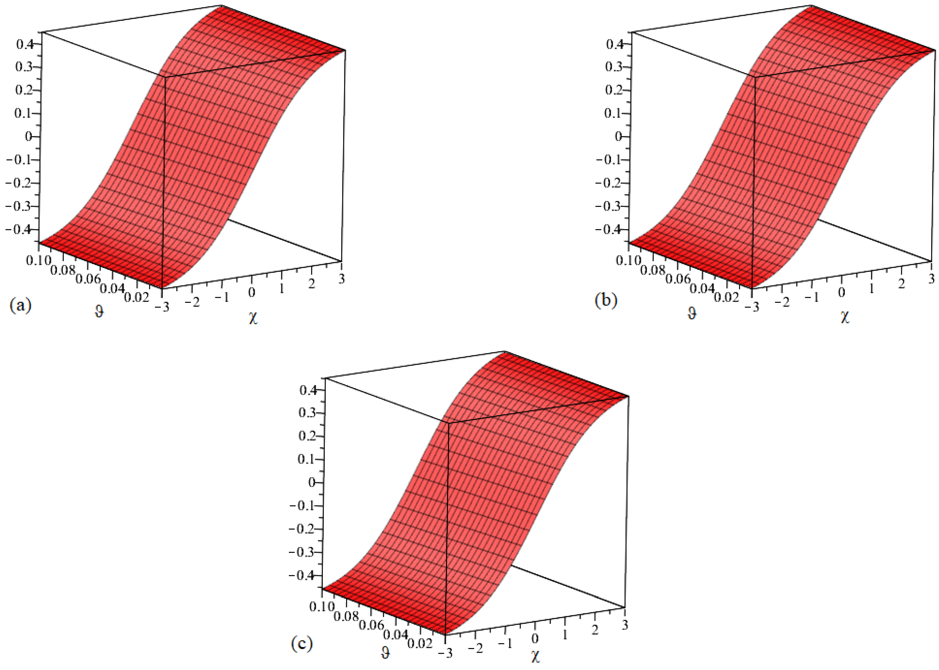
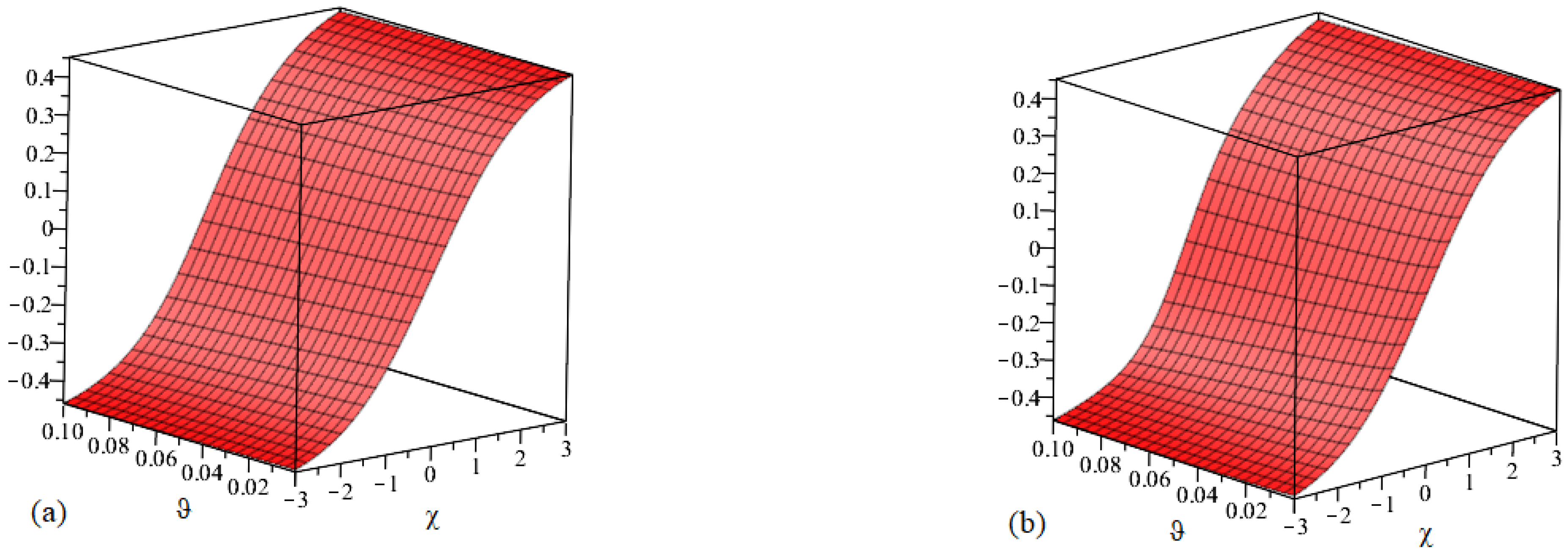
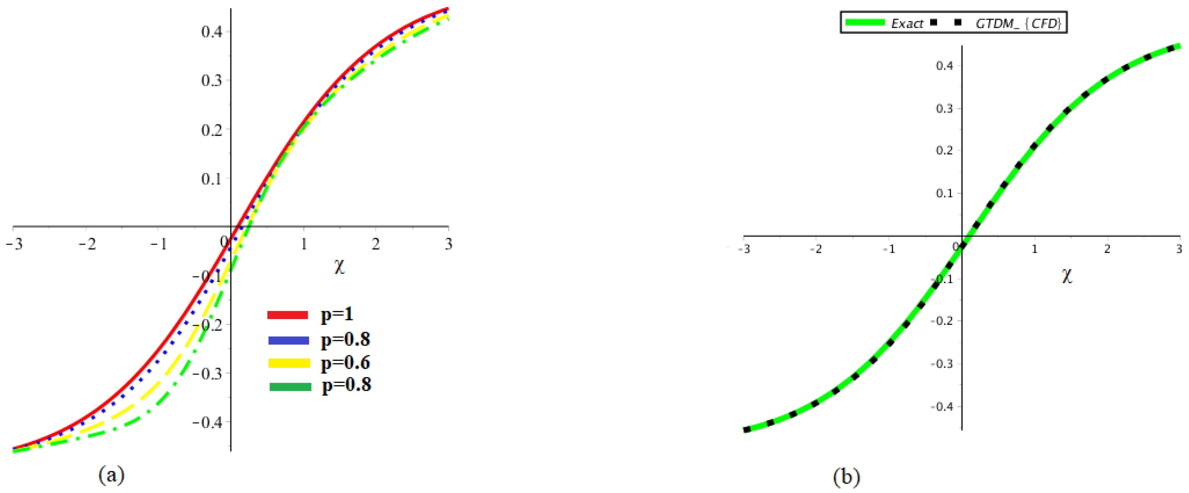
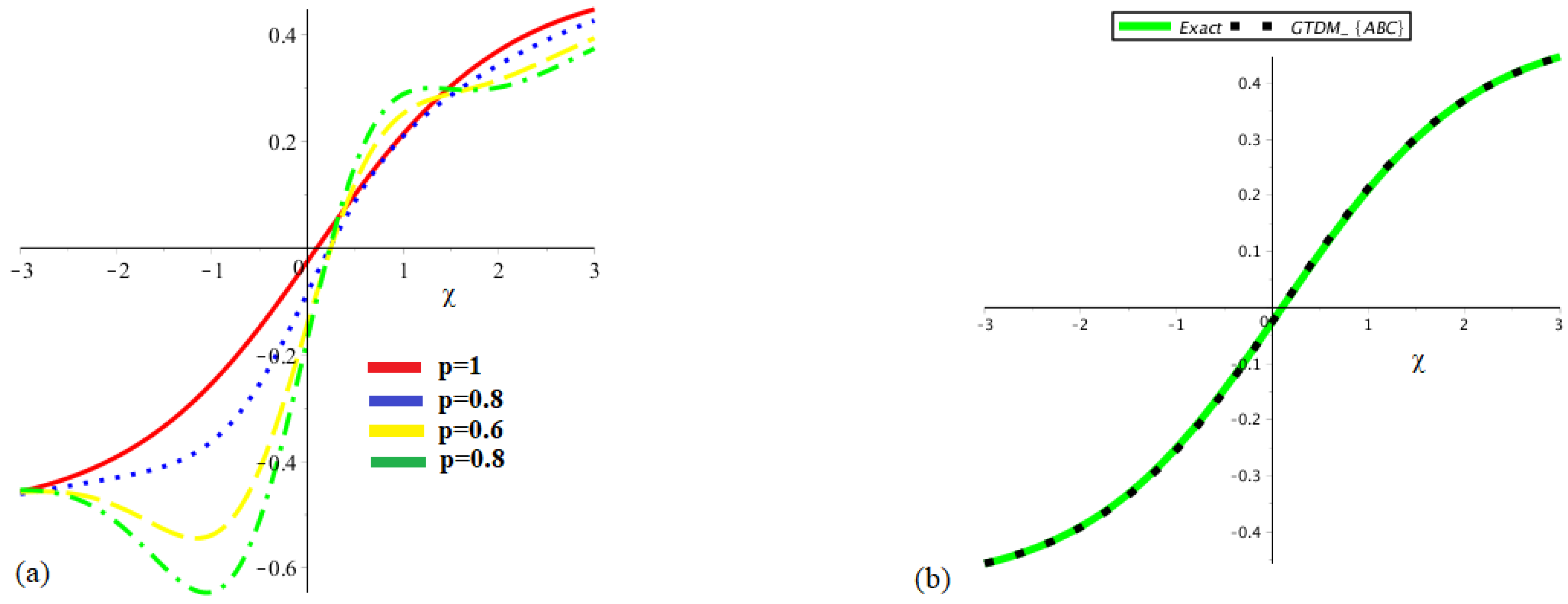
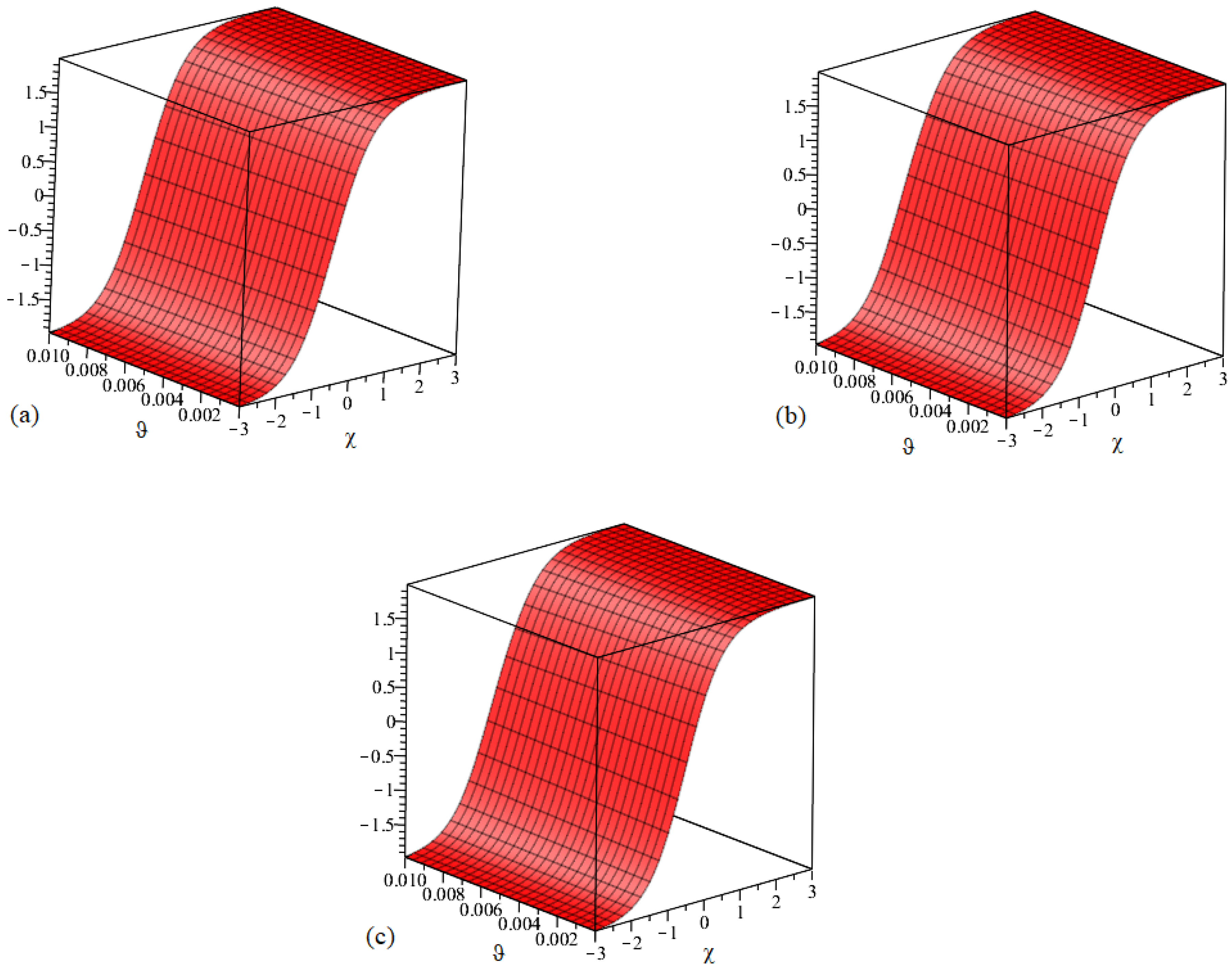
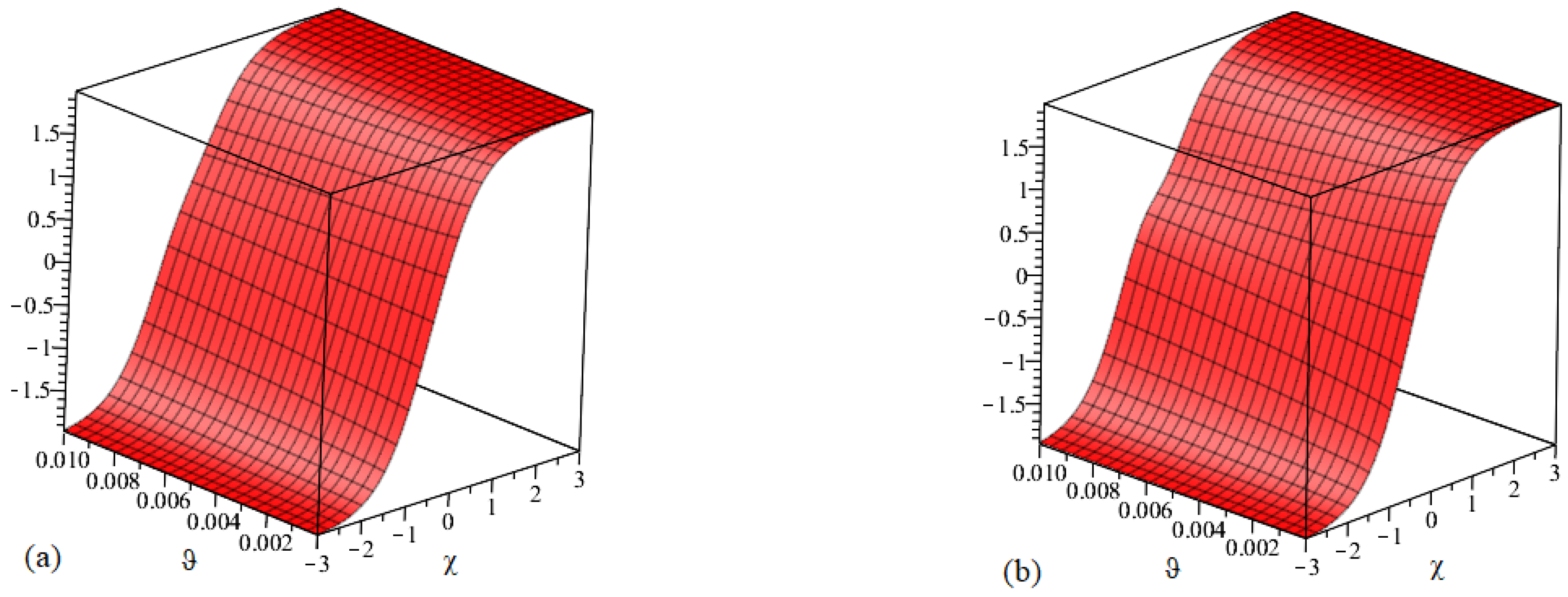
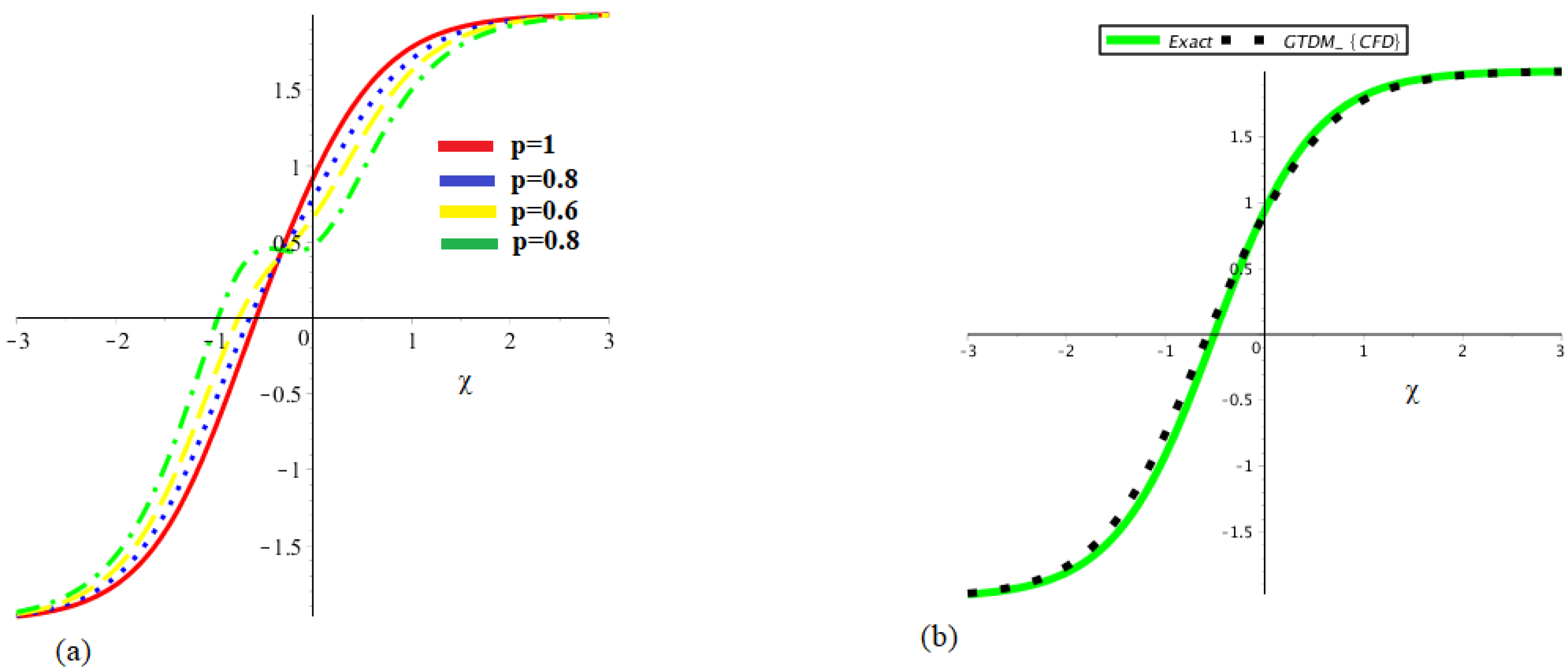
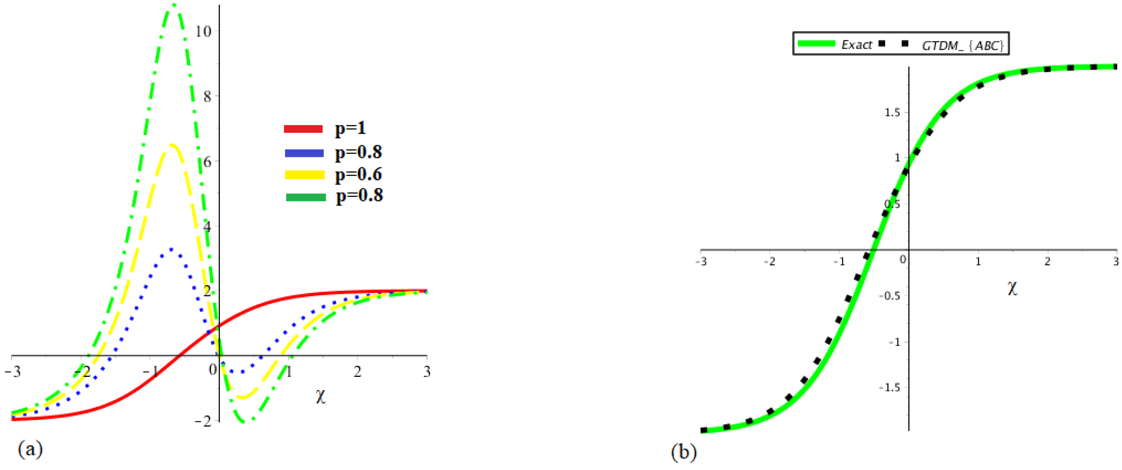
To figure out the distinctive dynamics of the fractional nonlinear shock waves, the approximations obtained for the two analyzed examples using the suggested technique have been computationally examined against the fractional-order parameter $\mathtt{p}$. We examined the fractional nonlinear structures given by these approximations against fractionality $\mathtt{p}$ in order to analyze their dynamics. The similarity between the precise result and the solution derived using GTDM under both operators is seen in Figure 1 for Example 1. The impact of the fractionality $\mathtt{p}$ on the shock wave profile under $CFD$ operator is shown in Figure 2 for Example 1. The impact of the fractionality $\chi$ on the shock wave profile under $CFD$ operator is shown in Figure 3 for example 1. Figure 4 and Figure 5 displays the two-dimensional shock wave profiles under both operators for various values of $\mathtt{p}$ as well as comparison of precise result with the solution derived for Example 1. This impact may reveal specific characteristics of the wave propagation dynamics that exact solutions for the integer case could not disclose. The achieved results demonstrated in Figure 1, Figure 2, Figure 3, Figure 4 and Figure 5 are drawn for a range of $\mathtt{p}$ values with $-3\le \chi \le 3$, and temporal variable $0\le \vartheta \le 0.1$.

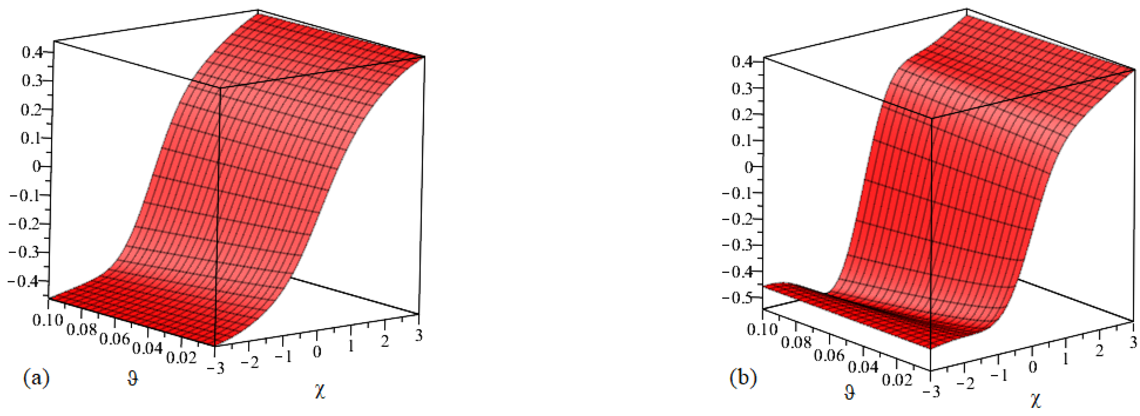
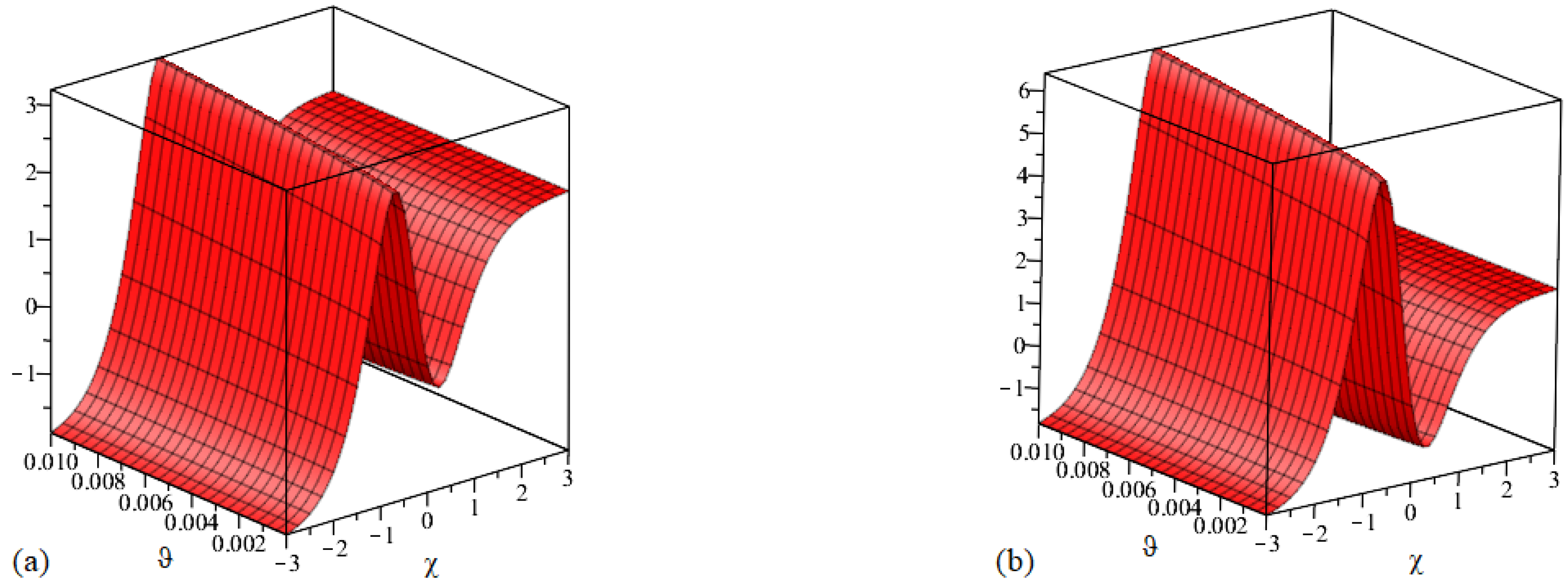
The similarity between the precise result and the solution derived using GTDM under both operators is seen in Figure 6 for Example 2. The impact of the fractionality $\mathtt{p}$ on the shock wave profile under $CFD$ operator is shown in Figure 7 for Example 2. The impact of the fractionality $\chi$ on the shock wave profile under $CFD$ operator is shown in Figure 8 for Example 2. Figure 9 and Figure 10 display the two-dimensional shock wave profiles under both operators for various values of $\mathtt{p}$ as well as a comparison of the precise result with the solution derived for Example 2. This impact may reveal specific characteristics of the wave propagation dynamics that exact solutions for the integer case could not disclose. The achieved results demonstrated in Figure 6, Figure 7, Figure 8, Figure 9 and Figure 10 are drawn for a range of $\mathtt{p}$ values with $-3\le \chi \le 3$, and temporal variable $0\le \vartheta \le 0.01$.

6.3. Physical Insights

The wave profiles of the fractional STO equation for various fractional orders $\mathtt{p}$ are shown in all of the figures. The classical shock wave profile is obtained for $\mathtt{p}=1$. The Caputo derivative’s power-law memory introduces damping and smoothing as $\mathtt{p}$ drops. This kernel provides a significant heredity influence that gradually decreases the shock-like pattern and reduces the amplitude, which is correlated with sub-diffusive transport where the impact of previous states gradually diminishes. The Atangana–Baleanu derivative’s nonlocal, non-singular kernel causes crossover effects with initial overshoot. Physically, this simulates systems in which long-range correlations are maintained, but memory effects degrade exponentially. As a result, the Caputo operator produces more dissipative behavior and quicker stabilization to the steady tanh-profile, whereas the ABC operator captures more prominent dispersion and pre-asymptotic oscillations in the STO dynamics. This is a reflection of how waves behave physically when they propagate across viscoelastic and heterogeneous media, where memory and nonlocal interactions change the wave front’s dispersion and steepness. The fact that the exact and approximate solutions match so well shows that GTDM maintains the physical properties of the fractional wave dynamics.

6.4. Accuracy and Convergence Validation

Table 1. Numerical simulation of our methodologies at different values of $\mathtt{p}$.

$\mathit{\vartheta }$	$\mathit{\chi }$	GTDMABC $(\mathtt{p}=\mathbf{0}.\mathbf{90})$	GTDMCFD $(\mathtt{p}=\mathbf{0}.\mathbf{90})$	GTDMABC $(\mathtt{p}=\mathbf{1})$	GTDMCFD $(\mathtt{p}=\mathbf{1})$	$\mathit{Exact}$ $(\mathtt{p}=\mathbf{1})$	$\mathit{Relative} \mathit{Error}$ $(\mathtt{p}=\mathbf{1})$	$\mathit{Residual} \mathit{Error}$ $(\mathtt{p}=\mathbf{1})$
	2	0.3684991487	0.3790641259	0.3797462198	0.3797462198	0.3797431376	8.11637 $\times {10}^{-6}$	0.0006382115567
	4	0.4792094218	0.4817138409	0.4818363090	0.4818363090	0.4818341977	4.38159 $\times {10}^{-6}$	−0.0004259050907
0.01	6	0.4971178932	0.4974852858	0.4975025886	0.4975025886	0.4975022294	7.22327 $\times {10}^{-7}$	$-7.15762\times {10}^{-5}$
	8	0.4996086573	0.4996589251	0.4996612807	0.4996612807	0.4996612306	1.00079 $\times {10}^{-7}$	$-9.95459\times {10}^{-6}$
	10	0.4999470138	0.4999538269	0.4999541459	0.4999541459	0.4999541391	1.40519 $\times {10}^{-8}$	$-1.35214\times {10}^{-6}$
	2	0.3632114116	0.3733821099	0.3755243424	0.3755243424	0.3754466418	2.06955 $\times {10}^{-4}$	$0.0036090961$
	4	0.4776602156	0.4806138198	0.4810565252	0.4810565252	0.4811090380	1.09149 $\times {10}^{-4}$	$-0.0021916588$
0.05	6	0.4968855297	0.4973281715	0.4973919930	0.4973919930	0.4974009322	1.79714 $\times {10}^{-5}$	$-0.0003509066$
	8	0.4995767729	0.4996375047	0.4996462168	0.4996462168	0.4996474622	2.49293 $\times {10}^{-6}$	$-0.0000484860$
	10	0.4999426907	0.4999509251	0.4999521055	0.4999521055	0.4999522746	3.37830 $\times {10}^{-7}$	$-0.0000065801$
	2	0.3595447103	0.3694375880	0.3723385670	0.3723385670	0.3721384337	5.37792 $\times {10}^{-4}$	$0.0062070429$
	4	0.4765053338	0.4797472714	0.4804110021	0.4804110021	0.4805449154	2.78669 $\times {10}^{-4}$	$-0.0035799653$
0.08	6	0.4967111860	0.4972022317	0.4972991868	0.4972991868	0.4973219908	4.58537 $\times {10}^{-5}$	$-0.0005530298$
	8	0.4995528302	0.4996202944	0.4996335527	0.4996335527	0.4996367297	6.35843 $\times {10}^{-6}$	$-0.0000760324$
	10	0.499939444	0.4999485929	0.4999503897	0.4999503897	0.4999508212	8.62815 $\times {10}^{-7}$	$-0.0000103114$
	2	0.3571683955	0.3668793294	0.3702054942	0.3702054942	0.3698915256	8.48812 $\times {10}^{-4}$	$0.0080797735$
	4	0.4757222875	0.4791411553	0.4799510015	0.4799510015	0.4801596942	4.34630 $\times {10}^{-4}$	$-0.0045352802$
0.1	6	0.4965925267	0.4971133213	0.4972324925	0.4972324925	0.4972680392	7.14836 $\times {10}^{-5}$	$-0.0006842373$
	8	0.4995365267	0.4996081295	0.4996244415	0.4996244415	0.4996293938	9.91202 $\times {10}^{-6}$	$-0.0000937521$
	10	0.4999372330	0.4999469441	0.4999491551	0.4999491551	0.4999498278	1.34634 $\times {10}^{-6}$	$-0.0000127087$

,

Table 2. Comparison of our methodology in terms of both operators with q-Homotopy analysis Elzaki transform method (q-HAETM) at various values of $\vartheta$ and $\chi$.

$\mathit{\vartheta }$	$\mathit{\chi }$	$\mathit{q}-\mathit{HAETM} \mathit{Error}$	GTDMCFD $\mathit{Error}$	GTDMABC $\mathit{Error}$
	5	2.8246 $\times {10}^{-7}$	9.2538753400 $\times {10}^{-9}$	9.2538753400 $\times {10}^{-9}$
	4	4.2905 $\times {10}^{-7}$	2.1158007320 $\times {10}^{-8}$	2.1158007320 $\times {10}^{-8}$
0.001	3	8.7092 $\times {10}^{-6}$	3.2425764750 $\times {10}^{-8}$	3.2425764750 $\times {10}^{-8}$
	2	5.7987 $\times {10}^{-5}$	3.0792074770 $\times {10}^{-8}$	3.0792074770 $\times {10}^{-8}$
	1	1.9745 $\times {10}^{-4}$	2.5578805190 $\times {10}^{-7}$	2.5578805190 $\times {10}^{-7}$
	5	8.1686 $\times {10}^{-7}$	5.0956382560 $\times {10}^{-10}$	5.0956382560 $\times {10}^{-10}$
	4	6.5000 $\times {10}^{-7}$	4.0144459660 $\times {10}^{-9}$	4.0144459660 $\times {10}^{-9}$
0.002	3	1.9479 $\times {10}^{-5}$	2.9585519280 $\times {10}^{-8}$	2.9585519280 $\times {10}^{-8}$
	2	1.2665 $\times {10}^{-4}$	2.0876796060 $\times {10}^{-7}$	2.0876796060 $\times {10}^{-7}$
	1	3.6421 $\times {10}^{-4}$	3.5897472240 $\times {10}^{-7}$	3.5897472240 $\times {10}^{-7}$

,

Table 3. Numerical simulation of our methodologies at different values of $\mathtt{p}$.

$\mathit{\vartheta }$	$\mathit{\chi }$	GTDMABC $(\mathtt{p}=\mathbf{0}.\mathbf{90})$	GTDMCFD $(\mathtt{p}=\mathbf{0}.\mathbf{90})$	GTDMABC $(\mathtt{p}=\mathbf{1})$	GTDMCFD $(\mathtt{p}=\mathbf{1})$	$\mathit{Exact}$ $(\mathtt{p}=\mathbf{1})$	$\mathit{Relative} \mathit{Error}$ $(\mathtt{p}=\mathbf{1})$	$\mathit{Residual} \mathit{Error}$ $(\mathtt{p}=\mathbf{1})$
	2	1.8886865680	1.9632362680	1.9681473390	1.9681473390	1.9737190220	2.82293 $\times {10}^{-3}$	$0.1748530620$
	4	1.9979101000	1.9993170340	1.9994097160	1.9994097160	1.9995155210	5.29156 $\times {10}^{-5}$	$0.0036103728$
0.01	6	1.9999617050	1.9999874880	1.9999891860	1.9999891860	1.9999911250	9.68757 $\times {10}^{-7}$	$6.62696\times {10}^{-5}$
	8	1.9999993000	1.9999997720	1.9999998030	1.9999998030	1.9999998370	1.70075 $\times {10}^{-8}$	$1.21381\times {10}^{-6}$
	10	1.9999999870	1.9999999960	1.9999999960	1.9999999960	1.9999999970	5.60287 $\times {10}^{-10}$	$2.22318\times {10}^{-8}$
	2	1.8520759530	1.9225568060	1.9378274350	1.9378274350	1.9638971920	1.32745 $\times {10}^{-2}$	$1.0042761053$
	4	1.9972191590	1.9985493220	1.9988375130	1.9988375130	1.9993328430	2.47747 $\times {10}^{-4}$	$0.0216903589$
0.05	6	1.9999490430	1.9999734190	1.9999787000	1.9999787000	1.9999877790	4.53879 $\times {10}^{-6}$	$0.0003984506$
	8	1.9999990680	1.9999995140	1.9999996110	1.9999996110	1.9999997760	8.30375 $\times {10}^{-8}$	$7.29827\times {10}^{-6}$
	10	1.9999999830	1.9999999910	1.9999999930	1.9999999930	1.9999999960	1.19856 $\times {10}^{-9}$	$1.33672\times {10}^{-7}$
	2	1.8268800090	1.8945606410	1.9150876090	1.9150876090	1.9542164220	2.00227 $\times {10}^{-2}$	$1.7418422075$
	4	1.9967436410	1.9980209680	1.9984083610	1.9984083610	1.9991519150	3.71935 $\times {10}^{-4}$	$0.0390623377$
0.08	6	1.9999403290	1.9999637370	1.9999708360	1.9999708360	1.9999844640	6.81399 $\times {10}^{-6}$	$0.0007180412$
	8	1.9999989080	1.9999993370	1.9999994670	1.9999994670	1.9999997150	1.24960 $\times {10}^{-7}$	$1.31522\times {10}^{-5}$
	10	1.9999999800	1.9999999880	1.9999999900	1.9999999900	1.9999999950	2.41770 $\times {10}^{-9}$	$2.40892\times {10}^{-7}$
	2	1.8106330470	1.8765080370	1.8999277720	1.8999277720	1.9463789650	2.38654 $\times {10}^{-2}$	$2.2760176295$
	4	1.9964370140	1.9976802720	1.9981222600	1.9981222600	1.9990048000	4.41489 $\times {10}^{-4}$	$0.0524536715$
0.1	6	1.9999347100	1.9999574930	1.9999655930	1.9999655930	1.9999817680	8.08753 $\times {10}^{-6}$	$0.0009646498$
	8	1.9999988050	1.9999992220	1.9999993710	1.9999993710	1.9999996650	1.47075 $\times {10}^{-7}$	$1.76694\times {10}^{-5}$
	10	1.9999999780	1.9999999850	1.9999999880	1.9999999880	1.9999999950	3.29712 $\times {10}^{-9}$	$3.23628\times {10}^{-7}$

and

Table 4. Comparison of our methodology in terms of both operators with HPM at different values of $\chi$.

$\mathit{\chi }$	$\mathit{HPM} \mathit{Error}$	GTDMCFD $\mathit{Error}$	GTDMABC $\mathit{Error}$
2	7.2096 $\times {10}^{-4}$	5.5716836560 $\times {10}^{-3}$	5.5716836560 $\times {10}^{-3}$
3	5.3361 $\times {10}^{-4}$	7.7845043750 $\times {10}^{-4}$	7.7845043750 $\times {10}^{-4}$
4	2.3942 $\times {10}^{-4}$	1.0580472040 $\times {10}^{-4}$	1.0580472040 $\times {10}^{-4}$
5	9.4126 $\times {10}^{-5}$	1.4327171050 $\times {10}^{-5}$	1.4327171050 $\times {10}^{-5}$
6	3.5453 $\times {10}^{-5}$	1.9385037590 $\times {10}^{-6}$	1.9385037590 $\times {10}^{-6}$
7	1.3154 $\times {10}^{-5}$	2.6178509530 $\times {10}^{-7}$	2.6178509530 $\times {10}^{-7}$
8	4.8545 $\times {10}^{-6}$	3.4014998880 $\times {10}^{-8}$	3.4014998880 $\times {10}^{-8}$
9	1.7879 $\times {10}^{-6}$	3.4981245280 $\times {10}^{-9}$	3.4981245280 $\times {10}^{-9}$
10	6.5802 $\times {10}^{-7}$	8.7942554240 $\times {10}^{-10}$	8.7942554240 $\times {10}^{-10}$

provide a detailed comparison of GTDM and actual solutions at various fractional orders $\mathtt{p}=$. The applied method achieves good numerical precision with mostly low absolute error and provides approximation results that are extremely close to the actual solution. Table 1 cites the approximated results obtained for different values of $\mathtt{p}$ using the technique under consideration. To verify the accuracy of the proposed algorithms, we compare the exact solution with the achieved result. In comparison to q-HAETM, Table 2 provides absolute errors at $\vartheta =0.001$ and $\vartheta =0.002$, respectively, indicating the accuracy of the approaches studied. Table 3 cites the approximated results obtained for different values of $\mathtt{p}$ using the technique under consideration. Table 4 examines absolute errors to compare the accuracy of the methods under consideration with those of other methods, specifically HPM. The achieved results demonstrate how well the suggested approach works with nonlinear fractional differential equations. Since the method under consideration requires fewer computations and effort than other approaches, they significantly improve the fields over current procedures. In the future, we hope to use these approaches to solve other nonlinear fractional PDEs that come across fields like biology, medicine, and engineering.

6.5. Error Analysis

Table 5. Statistical error analysis for Example 1 at $\mathtt{p}=1$.

$\mathit{\vartheta }$	Metric	Value
0.01	CPU Time	0.14 ms
	Max Relative Error	1.40519 $\times {10}^{-8}$
	Max Absolute Error	7.13206 $\times {10}^{-6}$
	Mean Relative Error	2.66688 $\times {10}^{-6}$
	Root Mean Square Error	3.75359 $\times {10}^{-6}$
0.05	CPU Time	0.14 ms
	Max Relative Error	3.37830 $\times {10}^{-7}$
	Max Absolute Error	9.58390 $\times {10}^{-6}$
	Mean Relative Error	6.73814 $\times {10}^{-5}$
	Root Mean Square Error	9.42150 $\times {10}^{-5}$
0.08	CPU Time	0.14 ms
	Max Relative Error	8.62815 $\times {10}^{-7}$
	Max Absolute Error	1.13772 $\times {10}^{-5}$
	Mean Relative Error	1.73907 $\times {10}^{-4}$
	Root Mean Square Error	2.41901 $\times {10}^{-4}$
0.1	CPU Time	0.14 ms
	Max Relative Error	1.34634 $\times {10}^{-6}$
	Max Absolute Error	1.25947 $\times {10}^{-5}$
	Mean Relative Error	2.73237 $\times {10}^{-4}$
	Root Mean Square Error	3.78704 $\times {10}^{-4}$

and

Table 6. Statistical error analysis for Example 2 at $\mathtt{p}=1$.

$\mathit{\vartheta }$	Metric	Value
0.01	CPU Time	0.15 ms
	Max Relative Error	5.60287 $\times {10}^{-10}$
	Max Absolute Error	1.00985 $\times {10}^{-8}$
	Mean Relative Error	5.75367 $\times {10}^{-4}$
	Root Mean Square Error	5.57268 $\times {10}^{-3}$
0.05	CPU Time	0.15 ms
	Max Relative Error	1.19856 $\times {10}^{-9}$
	Max Absolute Error	1.33462 $\times {10}^{-8}$
	Mean Relative Error	27053 $\times {10}^{-3}$
	Root Mean Square Error	2.6074 $\times {10}^{-2}$
0.08	CPU Time	0.15 ms
	Max Relative Error	2.41770 $\times {10}^{-9}$
	Max Absolute Error	1.52695 $\times {10}^{-8}$
	Mean Relative Error	4.08032 $\times {10}^{-3}$
	Root Mean Square Error	3.91358 $\times {10}^{-2}$
0.1	CPU Time	0.15 ms
	Max Relative Error	3.29712 $\times {10}^{-9}$
	Max Absolute Error	1.71545 $\times {10}^{-8}$
	Mean Relative Error	4.86303 $\times {10}^{-3}$
	Root Mean Square Error	4.64595 $\times {10}^{-2}$

summarize the statistical error metrics for the integer-order case ($\mathtt{p}=1$) of the two problems. The CPU time, maximum relative error, maximum absolute error, mean relative error, and root mean square error are calculated for both problems. These metrics confirm that the proposed method (which produces identical numerical results) achieves excellent accuracy. The CPU times of both problems are virtually similar (nearly 0.15 ms), which is an indication that the proposed method has a low computational cost. The quantitative findings in both tables reveal that the proposed method is highly consistent with the actual solution, as the arguments provided above in the manuscript.

6.6. Convergence Analysis

By assessing the truncation errors over different parameters ($\chi ,\vartheta$) and fractional orders ($\mathtt{p}$), the convergence behavior of GTDM for each example may be examined. Table 1 illustrates how the relative error quickly decreases from $8.11637\times {10}^{-6}$ at $\chi =2$ to $1.40519\times {10}^{-8}$ at $\chi =10$ for a given time scale ($\vartheta =0.01$). This shows that as $\chi$ goes more from the origin into asymptotic stability regimes, the spatial convergence rate increases dramatically. The approximation solutions seamlessly return to the standard precise solution when $\mathtt{p}\to 1$. Table 2 demonstrates that GTDM yields remarkably low errors (${10}^{-8}$ to ${10}^{-7}$) for small time intervals ($\vartheta =0.001$), outperforming competing approaches such as q-HAETM by up to three orders of magnitude. Table 3 shows continuous convergence for the more complicated structure in Example 2. The relative error decreases exponentially from $2.82293\times {10}^{-3}$ ($\chi =2$) to $5.60287\times {10}^{-10}$ ($\chi =10$) at $\vartheta =0.01$.

6.7. Stability Analysis

The type of fractional derivative operators used (ABC vs. CFD) has a significant impact on the numerical scheme’s stability. Table 1 and Table 3 show that ${\mathrm{GTDM}}_{\mathrm{ABC}}$ and ${\mathrm{GTDM}}_{\mathrm{CFD}}$ produce the same numerical results for $\mathtt{p}=1$. This suggests that when the fractional order becomes closer to unity, both operators maintain the computational stability limitations of the classical system. In Example 2, the relative error is tightly controlled (${10}^{-2}$), even though the residual error spikes significantly at localized strong gradients (e.g., $ResidualError=2.276$ at $\vartheta =0.1,\chi =2$). The ABC operator’s nonlocal kernel, which is based on Mittag-Leffler functions, adds memory features that reduce numerical oscillations while maintaining $L_2$ and $L_{\infty }$ stability configurations across extended propagating computations.

6.8. Computational Efficiency

The effectiveness of GTDM is assessed in comparison to current semi-analytical techniques such as the q-HAETM and the HPM. Computing lengthy Adomian polynomials or homotopy embedding steps is a requirement of classical perturbation methods. By employing a direct decomposition technique, GTDM gets around this problem and evaluates high-order iterations (such as the lengthy ${\mathtt{z}}_2$ components produced in Example 2 with much less CPU time and memory usage.

Table 7. Asymptotic error profiles.

Metric/Method	HPM (Table 4)	q-HAETM (Table 2)	GTDM (ABC/CFD)
Error Range ($\chi =2$)	$7.20\times {10}^{-4}$	$5.79\times {10}^{-5}$	$5.57\times {10}^{-3}$
Error Range ($\chi =10$)	$6.58\times {10}^{-7}$	$1.97\times {10}^{-4}$	$8.79\times {10}^{-10}$
Asymptotic Efficiency	Linear / Flat	Degrades near boundary	High (Scales with $\chi$)

illustrates how although HPM produces a slightly smaller error close to the source core ($\chi =2$), its accuracy only reaches ${10}^{-7}$ at $\chi =10$. On the other hand, GTDM grows continuously and perfectly captures asymptotic decay patterns down to ${10}^{-10}$.

6.9. Limitations and Future Work Directions

The suggested GTDM has many limitations compared to its effectiveness. Strong nonlinear or more lengthy simulations may require more computing power because the solution is found as a truncated series, the accuracy of which depends on the number of retained terms. When addressing coupled systems and higher-order nonlinearities, the algebraic complexity of Adomian polynomials can also grow rapidly. Furthermore, the present approach, which is primarily suited to deterministic cases, assumes smooth initial conditions and constant fractional order.

We are currently focusing on a series of upcoming studies using GTDM to explore various fractional evolutionary wave equations, such as the family of the fractional KdV equation, the family of the fractional Kawahara equation, and the family of the fractional nonlinear Schrödinger equation associated with plasma physics to model nonlinear phenomena that appear and propagate in different plasma systems, such as solitons, shocks, cnoidal waves, and rogue waves, because of the ease and straightforward execution of GTDM to investigate various types of fractional nonlinear PDEs and their promising results. Future additions of operators like $\varphi$-Caputo derivative, Caputo–Fabrizio derivative, Katugampola derivative, and Comformable derivative will be highly advantageous given the benefits of the current operators. We assume that our approach will be applied in the future to successfully and efficiently address further fractional differential issues in scientific fields. This work is advantageous and will lead to new avenues in science and engineering.

7. Conclusions

In this study, we have shown how to use the effective GTDM under the Caputo and Atangana–Baleanu–Caputo (ABC) fractional operators to solve the nonlinear time-fractional STO equation. In order to demonstrate the importance and efficacy of the schemes under consideration, we have looked at two cases with different initial solutions. The computed study findings are shown in tables and graphs. The tables and graphs demonstrate that the approximate solution of the issue converges to its precise answer when the value of $\mathtt{p}$ gets closer to the problem’s classical value of 1. Numerical simulations that are presented ensure more accurate outcomes. By taking into account various initial approximations, this study is able to investigate the fractional behavior of the nonlinear STO problem and its solution in depth. The suggested method is successful in providing a nonlocal influence, a critical convergence zone, and a straightforward solution. In conclusion, the developed approximations for the suggested issues exhibit greater stability throughout the whole study domain along with excellent accuracy. As a result, the results show how effective the methods are for assessing different nonlinear FDEs. However, compared to the other two approaches, the GTDM involves less work and fewer computations. Therefore, we plan to use the GTDM to solve other fractional strong nonlinear partial differential equations that are essential to model different engineering, biology, chemistry, and physics problems, especially evolutionary wave equations that are used to represent nonlinear plasma waves.

References

1. Kilbas, A.A.; Srivastava, H.M.; Trujillo, J.J. Theory and Applications of Fractional Differential Equations; North-Holland Mathematics Studies; Elsevier Science: Amsterdam, The Netherlands, 2006. [Google Scholar]
2. Podlubny, I. Fractional Differential Equations; Academic Press: San Diego, CA, USA, 1999. [Google Scholar]
3. Cruz-Duarte, J.M.; Rosales-Garcia, J.; Correa-Cely, C.R.; Garcia-Perez, A.; Avina-Cervantes, J.G. A closed form expression for the Gaussian-based Caputo-Fabrizio fractional derivative for signal processing applications. Commun. Nonlinear Sci. Numer. Simul. 2018, 61, 138–148. [Google Scholar] [CrossRef]
4. Baleanu, D.; Wu, G.C.; Zeng, S.D. Chaos analysis and asymptotic stability of generalized Caputo fractional differential equations. Chaos Solitons Fractals 2017, 102, 99–105. [Google Scholar] [CrossRef]
5. Drapaca, C.S.; Sivaloganathan, S. A fractional model of continuum mechanics. J. Elast. 2012, 107, 105–123. [Google Scholar] [CrossRef]
6. Jajarmi, A.; Baleanu, D. On the fractional optimal control problems with a general derivative operator. Asian J. Control 2021, 23, 1062–1071. [Google Scholar] [CrossRef]
7. Turalska, M.; West, B.J. Fractional dynamics of individuals in complex networks. Front. Phys. 2018, 6, 110. [Google Scholar] [CrossRef]
8. AlBaidani, M.M. Comparative study of the nonlinear fractional generalized Burger-Fisher equations using the homotopy perturbation transform method and new iterative transform method. Fractal Fract. 2025, 9, 390. [Google Scholar] [CrossRef]
9. Chauhan, J.P.; Khirsariya, S.R.; Hathiwala, M.B. A caputo-type fractional-order model for the transmission of chlamydia disease. Contemp. Math. 2024, 5, 2134–2157. [Google Scholar]
10. Jassim, H.K.; Khafif, S.A. SVIM for solving Burger’s and coupled Burger’s equations of fractional order. Prog. Fract. Differ. Appl. 2021, 7, 73–78. [Google Scholar]
11. Khirsariya, S.; Rao, S.; Chauhan, J. Solution of fractional modified Kawahara equation: A semi-analytic approach. Math. Appl. Sci. Eng. 2023, 4, 264–284. [Google Scholar] [CrossRef]
12. Zada, L.; Nawaz, R.; Jamshed, W.; Ibrahim, R.W.; Tag El Din, E.S.M.; Raizah, Z.; Amjad, A. New optimum solutions of nonlinear fractional acoustic wave equations via optimal homotopy asymptotic method-2 (OHAM-2). Sci. Rep. 2022, 12, 18838. [Google Scholar] [CrossRef]
13. Khirsariya, S.R.; Rao, S.B.; Hathiwala, G.S. Investigation of fractional diabetes model involving glucose-insulin alliance scheme. Int. J. Dyn. Control 2024, 12, 1–14. [Google Scholar] [CrossRef]
14. Huang, G.; Qin, H.Y.; Chen, Q.; Shi, Z.; Jiang, S.; Huang, C. Research on application of fractional calculus operator in image underlying processing. Fractal Fract. 2024, 8, 37. [Google Scholar] [CrossRef]
15. Xin, Z.; Jing, Z.; Wenru, L.; Wenbo, X. Research on fractional sliding mode synchronous control of robotic arms under uncertain disturbance. At. Control Comput. Sci. 2021, 55, 26–37. [Google Scholar]
16. Wang, X.; Petru, M.; Xia, L. Modelling the dynamical behaviour of the flax fibre rainforced composite after water using a modified Huet-Sayegh viscoelastic model with fractional derivatives. Constr. Build. Mater. 2021, 290, 122879. [Google Scholar] [CrossRef]
17. AlBaidani, M.M.; Alzahrani, R. A Computational Analysis of Nonlinear Fractional Coupled System of Boussinesq–Burger Equations with the Non-Singular Kernel. Axioms 2026, 15, 172. [Google Scholar] [CrossRef]
18. Veeresha, P.; Prakasha, D.G.; Baskonus, H.M. New numerical surfaces to the mathematical model of cancer chemotherapy effect in Caputo fractional derivatives. Chaos 2019, 29, 013119. [Google Scholar] [CrossRef] [PubMed]
19. El Mfadel, A.; Melliani, S.; Elomari, M.H. A note on the stability analysis of fuzzy nonlinear fractional differential equations involving the Caputo fractional derivative. Int. J. Math. Math. Sci. 2021, 2021, 7488524. [Google Scholar] [CrossRef]
20. AlBaidani, M.M.; Alzahrani, R. Insights into the time-fractional nonlinear KdV-type equations under non-singular Kernel operators. Symmetry 2026, 18, 391. [Google Scholar] [CrossRef]
21. AlBaidani, M.M. Mathematical analysis of fractional-order convection–reaction–diffusion equations under the Caputo fractional derivative. Front. Phys. 2026, 14, 1762827. [Google Scholar] [CrossRef]
22. Podlubny, I. Fractional Differential Equations: An Introduction to Fractional Derivatives, Fractional Differential Equations, to Methods of Their Solution and Some of Their Applications; Elsevier: Amsterdam, The Netherlands, 1998; Volume 198. [Google Scholar]
23. Caputo, M.; Fabrizio, M. A new definition of fractional derivative without singular kernel, Progress in Fractional Differentiation. Applications 2015, 1, 73–85. [Google Scholar]
24. Goufo, E.F.D.; Pene, M.K.; Mwambakana, J.N. Duplication in a model of rock fracture with fractional derivative without singular kernel. Open Math. 2015, 13, 000010151520150078. [Google Scholar] [CrossRef]
25. Hristov, J. Transient heat diffusion with a non-singular fading memory: From the Cattaneo constitutive equation with Jeffrey’s kernel to the Caputo-Fabrizio time-fractional derivative. Therm. Sci. 2016, 20, 757–762. [Google Scholar] [CrossRef]
26. Moore, E.J.; Sirisubtawee, S.; Koonprasert, S.; Caputo-Fabrizio, A. Fractional differential equation model for HIV/AIDS with treatment compartment. Adv. Differ. Equ. 2019, 2019, 1–20. [Google Scholar] [CrossRef]
27. Atangana, A.; Baleanu, D. New fractional derivatives with nonlocal and non-singular kernel: Theory and application to heat transfer model. arXiv 2016, arXiv:1602.03408. [Google Scholar] [CrossRef]
28. Ghanbari, B.; Atangana, A. A new application of fractional Atangana–Baleanu derivatives: Designing ABC-fractional masks in image processing. Phys. A Stat. Mech. Its Appl. 2020, 542, 123516. [Google Scholar] [CrossRef]
29. Meena, M.; Purohit, M.; Purohit, S.D.; Nisar, K.S. A novel investigation of the hepatitis B virus using a fractional operator with a non-local kernel. Partial Differ. Equ. Appl. Math. 2023, 8, 100577. [Google Scholar] [CrossRef]
30. Le, Q.H.; Ali, Q.; Al-Khaled, K.; Amir, M.; Riaz, S.; Khan, S.U.; Abdelmalek, Z.; Tlili, I. Study of hybrid nanofluid containing graphene oxide and molybdenum disulfide nanoparticles with engine oil base fluid: A non-singular fractional approach. Ain Shams Eng. J. 2024, 15, 102317. [Google Scholar] [CrossRef]
31. Shehadeh, A.; El-Ajou, A.; Burqan, A.; Eriqat, T. Wave Soliton Solutions for Conformable-Fractional Partial Differential Equations. Fractals 2026, 2650044. [Google Scholar] [CrossRef]
32. El-Ajou, A.; Burqan, A. An innovative analytical method for solving the fractional caudrey dodd gibbon equation. Fractals 2025, 33, 2550058. [Google Scholar] [CrossRef]
33. Eltayeb, H.; Abdalla, Y.T.; Bachar, I.; Khabir, M.H. Fractional telegraph equation and its solution by natural transform decomposition method. Symmetry 2019, 11, 334. [Google Scholar] [CrossRef]
34. Mahgoub, M.; Sedeeg, A. A comparative study for solving nonlinear fractional heat-like equations via Elzaki transform. Br. J. Math. Comput. Sci. 2016, 19, 1–12. [Google Scholar] [CrossRef]
35. Jena, R.M.; Chakraverty, S. Solving time-fractional Navier-Stokes equations using homotopy perturbation Elzaki transform. SN Appl. Sci. 2019, 1, 16. [Google Scholar] [CrossRef]
36. AlBaidani, M.M.; Alzahrani, R. A novel approach to solving generalised nonlinear dynamical systems within the Caputo operator. Fractal Fract. 2025, 9, 503. [Google Scholar] [CrossRef]
37. Oqielat, M.A.N.; Eriqat, T.; Al-Zhour, Z.; Ogilat, O.; El-Ajou, A.; Hashim, I. Construction of fractional series solutions to nonlinear fractional reaction-diffusion for bacteria growth model via Laplace residual power series method. Int. J. Dyn. Control 2023, 11, 520–527. [Google Scholar] [CrossRef]
38. AlBaidani, M.M.; Alzahrani, R. Novel approximations to the non-linear fractional Belousov-Zhabotinsky reaction in the frame of Caputo operator. Bound. Value Probl. 2026, 2026, 36. [Google Scholar] [CrossRef]
39. AlBaidani, M.M. Analytical insight into some fractional nonlinear dynamical systems involving the Caputo fractional derivative operator. Fractal Fract. 2025, 9, 320. [Google Scholar] [CrossRef]
40. Bishehniasar, M.; Salahshour, S.; Ahmadian, A.; Ismail, F.; Baleanu, D. An accurate approximate-analytical technique for solving time-fractional partial differential equations. Complexity 2017, 2017, 8718209. [Google Scholar] [CrossRef]
41. Odibat, Z.; Momani, S.; Xu, H. A reliable algorithm of homotopy analysis method for solving nonlinear fractional differential equations. Appl. Math. Model. 2010, 34, 593–600. [Google Scholar] [CrossRef]
42. El-Ajou, A.; Shqair, M.; Ghabar, I.; Burqan, A.; Saadeh, R. A solution for the neutron diffusion equation in the spherical and hemispherical reactors using the residual power series. Front. Phys. 2023, 11, 1229142. [Google Scholar] [CrossRef]
43. Zayed, E.M.; Amer, Y.A.; Shohib, R.M. The fractional complex transformation for nonlinear fractional partial differential equations in the mathematical physics. J. Assoc. Arab Univ. Basic Appl. Sci. 2016, 19, 59–69. [Google Scholar] [CrossRef]
44. El-Ajou, A.; Arqub, O.A.; Momani, S. Approximate analytical solution of the nonlinear fractional KdV-Burgers equation: A new iterative algorithm. J. Comput. Phys. 2015, 293, 81–95. [Google Scholar] [CrossRef]
45. Wu, G.Z.; Yu, L.J.; Wang, Y.Y. Fractional optical solitons of the space-time fractional nonlinear Schrödinger equation. Optik 2020, 207, 164405. [Google Scholar] [CrossRef]
46. Moumen, A.; Shafqat, R.; Alsinai, A.; Boulares, H.; Cancan, M.; Jeelani, M.B. Analysis of fractional stochastic evolution equations by using Hilfer derivative of finite approximate controllability. AIMS Math. 2023, 8, 16094–16114. [Google Scholar] [CrossRef]
47. Chen, A. Multi-kink solutions and soliton fission and fusion of Sharma-Tasso-Olver equation. Phys. Lett. A 2010, 374, 2340–2345. [Google Scholar] [CrossRef]
48. Hamdi, M.S.; Yaseen, S.R.; Al-Saphory, R.A.; Zerrik, E.H. A New Technique for Solving A Fractional Sharma-Tasso-Olever Equation. Iraqi J. Sci. 2024, 3378–3394. [Google Scholar] [CrossRef]
49. Butt, A.R.; Zaka, J.; Akgül, A.; El Din, S.M. New structures for exact solution of nonlinear fractional Sharma–Tasso–Olver equation by conformable fractional derivative. Results Phys. 2023, 50, 106541. [Google Scholar] [CrossRef]
50. Kumar, A. An efficient analytical method for the fractional order Sharma–Tasso–Olever equation by means of the Caputo–Fabrizio derivative. In Computation and Modeling for Fractional Order Systems; Academic Press: Cambridge, MA, USA, 2024; pp. 29–39. [Google Scholar]
51. Jafari, H. A new general integral transform for solving integral equations. J. Adv. Res. 2020, 32, 133–138. [Google Scholar] [CrossRef]
52. Adomian, G. A review of the decomposition method in applied mathematics. J. Math. Anal. Appl. 1988, 135, 501–544. [Google Scholar] [CrossRef]
53. Adomian, G. Solving Frontier Problems of Physics: The Decomposition Method; Springer Science & Business Media: Berlin/Heidelberg, Germany, 2013; Volume 60. [Google Scholar]
54. Molliq, Y.; Noorani, M.S.M.; Hashim, I. Variational iteration method for fractional heat-and wave-like equations. Nonlinear Anal. Real. World Appl. 2009, 10, 1854–1869. [Google Scholar] [CrossRef]
55. Debnath, L.; Bhatta, D. Integral Transforms and Their Applications; CRC Press: Boca Raton, FL, USA, 2014. [Google Scholar]
56. Jarad, F.; Abdeljawad, T. A modified Laplace transform for certain generalized fractional operators. Results Nonlin. Anal. 2018, 1, 88–98. [Google Scholar]
57. Belgacem, F.B.M.; Karaballi, A.A. Sumudu transform fundamental properties investigations and applications. Int. J. Stoch. Anal. 2006, 2006, 091083. [Google Scholar]
58. Aboodh, K.S. The new integral transform Aboodh transform. Glob. J. Pure Appl. Math. 2013, 9, 35–43. [Google Scholar]
59. Ahmadi, S.A.P.; Hosseinzadeh, H.; Cherati, A.Y. A new integral transform for solving higher order linear ordinary differential equations. Nonlinear Dyn. Syst. Theory 2019, 19, 243–252. [Google Scholar] [CrossRef]
60. Ahmadi, S.A.P.; Hosseinzadeh, H.; Cherati, A.Y. A new integral transform for solving higher order linear ordinary Laguerre and Hermite differential equations. Int. J. Appl. Comput Math. 2019, 5, 142. [Google Scholar] [CrossRef]
61. Elzaki, T.M. The new integral transform Elzaki Transform. Glob. J. Pure Appl. Math. 2011, 7, 57–64. [Google Scholar]
62. Khan, Z.H.; Khan, W.A. N-transform properties and applications. NUST J. Eng. Sci. 2008, 1, 127–133. [Google Scholar]
63. Abdelrahim Mahgoub, M.M. The new integral transform mohand transform. Adv. Theor. Appl. Math. 2017, 12, 11320. [Google Scholar]
64. Abdelrahim Mahgoub, M.M. The new integral transform sawi transform. Adv. Theor. Appl. Math. 2019, 14, 81–87. [Google Scholar]
65. Kamal, H.; Sedeeg, A. The new integral transform Kamal transform. Adv. Theor. Appl. Math. 2016, 11, 451–458. [Google Scholar]
66. Kim, H. On the form and properties of an integral transform with strength in integral transforms. Far East J. Math. Sci. 2017, 102, 2831–2844. [Google Scholar] [CrossRef]
67. Kim, H. The intrinsic structure and properties of Laplace-typed integral transforms. Math. Prob. Eng. 2017, 2017, 1762729. [Google Scholar] [CrossRef]
68. Meddahi, M.; Jafari, H.; Ncube, M.N. New general integral transform via Atangana-Baleanu derivatives. Adv. Diff. Equ. 2021, 2021, 2021385. [Google Scholar] [CrossRef]
69. Atangana, A.; Koca, I. Chaos in a simple nonlinear system with Atangana–Baleanu derivatives with fractional order. Chaos Solit. Fract. 2016, 89, 447–454. [Google Scholar] [CrossRef]
70. Yavuz, M.; Abdeljawad, T. Nonlinear regularized long-wave models with a new integral transformation applied to the fractional derivative with power and Mittag-Leffler kernel. Adv. Differ. Equ. 2020, 2020, 367. [Google Scholar] [CrossRef]
71. Bokhari, A.; Baleanu, D.; Belgacema, R. Application of Shehu transform to Atangana-Baleanu derivatives. J. Math. Comput. Sci. 2020, 20, 101–107. [Google Scholar] [CrossRef]
72. Haubold, H.J.; Mathai, A.M.; Saxena, R.K. Mittag-Leffler functions and their applications. J. Appl. Math. 2011, 2011, 298628. [Google Scholar] [CrossRef]
73. El-Kalla, I. Convergence of the Adomian method applied to a class of nonlinear integral equations. Appl. Math. Lett. 2008, 21, 372–376. [Google Scholar] [CrossRef]
74. Adomian, G.; Rach, R. Modified adomian polynomials. Math. Comput. Model. 1996, 24, 39–46. [Google Scholar] [CrossRef]
Figure 1. Surface plot of the (a) accurate, (b) GTDMCFD and (c) GTDMABC solutions at p = 1 .
Symmetry 18 01005 g001
Figure 2. Surface plot of GTDMCFD solution when (a) p = 0.8 and (b) p = 0.6 .
Symmetry 18 01005 g002
Figure 3. Surface plot of GTDMABC solution when (a) p = 0.8 and (b) p = 0.6 .
Symmetry 18 01005 g003
Figure 4. 2D surface plot of GTDMCFD solution at (a) various values of p and (b) comparison of accurate with the approximate solution.
Symmetry 18 01005 g004
Figure 5. 2D surface plot of GTDMABC solution at (a) various values of p and (b) comparison of accurate with the approximate solution.
Symmetry 18 01005 g005
Figure 6. Surface plot of the (a) accurate, (b) GTDMCFD and (c) GTDMABC solutions at p = 1 .
Symmetry 18 01005 g006
Figure 7. Surface plot of GTDMCFD solution when (a) p = 0.8 and (b) p = 0.6 .
Symmetry 18 01005 g007
Figure 8. Surface plot of GTDMABC solution when (a) p = 0.8 and (b) p = 0.6 .
Symmetry 18 01005 g008
Figure 9. 2D surface plot of GTDMCFD solution at (a) various values of p and (b) comparison of accurate with the approximate solution.
Symmetry 18 01005 g009
Figure 10. 2D surface plot of GTDMABC solution at (a) various values of p and (b) comparison of accurate with the approximate solution.
Symmetry 18 01005 g010