Series Arc Fault Detection Using Differential Higher-Order Cumulants and Symmetric Stacked Autoencoder

Abstract

In low-voltage distribution systems, series arc faults caused by poor contact and loose connections are a leading cause of electrical fires. Due to the negative resistance characteristics of arcs, such faults are difficult to detect using conventional overcurrent or leakage protectors. Existing detection methods predominantly rely on wavelet-based feature extraction or threshold-based classifiers. Wavelet transforms require predefined basis functions and lack adaptability to non-stationary current signals from appliances such as induction cookers. Threshold-based classifiers produce excessive false alarms under varying load conditions, as normal non-stationary load waveforms share high-frequency characteristics with arc fault signatures. As a result, existing arc fault protectors exhibit high false alarm rates, limiting practical deployment. To address these limitations, this study proposes a method for diagnosing low-voltage series arc faults based on differential-sliding window higher-order cumulants (HoCs) and stacked autoencoders (SAEs). The method first employs a differential-sliding time window approach to extract HoC features from current signals across seven typical loads, establishing a feature vector database for arc fault patterns. A symmetric stacked autoencoder (SAE) is constructed, trained using layer-wise pretraining to optimize hyperparameters and select the model with the best generalization performance. Experimental results demonstrate that the proposed method achieves a detection accuracy of 96.4% with a false alarm rate of 0% across all tested loads.

1. Introduction

Fire safety remains a critical public concern worldwide. According to the National Fire and Rescue Administration of China, approximately 552,000 fire incidents were reported in the first half of 2025, resulting in 1084 fatalities and property losses amounting to 4.08 billion RMB. Among all identified causes of fire, electrical faults rank as the leading contributor, accounting for 25.4% of all incidents—roughly 140,000 cases—surpassing other factors such as careless use of fire (20.7%), smoking (18.7%), and unextinguished embers (18.6%) [1].

Arc faults are one of the most common causes of electrical fires. When an electrical arc occurs, the high temperature it generates can easily ignite nearby flammable materials. In particular, series arc faults are especially dangerous because they do not cause a significant change in current, making them difficult to detect with conventional circuit breakers or residual current devices (RCDs). As a result, arc faults often remain unnoticed until a fire has already broken out, posing a serious threat to life and property safety [2]. This highlights the urgent need for developing effective arc fault diagnosis technologies capable of detecting series arc faults at an early stage.

Depending on their locations relative to the load in the circuit, arc faults can be classified into three types: series arc faults, parallel arc faults, and ground arc faults. Among these, parallel and ground arc faults are easier to detect. In contrast, due to the branch circuit load and the inherent negative voltage-current characteristic of series arc faults, the root mean square (RMS) current of a series arc fault is generally comparable to, or even slightly lower than, the normal rated load current. Moreover, series arc faults do not generate residual current, and consequently, conventional overcurrent protection devices and ground fault circuit interrupters (GFCIs) are unable to identify series arc faults within circuits [3]. Arc fault diagnosis encompasses several research directions, including but not limited to: (1) integrating information from arc flash, acoustic noise, electromagnetic radiation, temperature, voltage, and current via multi-parameter fusion to establish comprehensive detection models; (2) employing deep learning and other advanced techniques to autonomously extract hierarchical features of arc faults and enable identification through big data analysis; (3) providing early warnings of arc faults based on precursor phenomena generated during arc initiation, such as ultrasonic waves emitted by air breakdown; (4) developing advanced diagnostic algorithms for arc fault detection; (5) and constructing comprehensive databases of arc fault characteristics.

Arc faults are accompanied by arc sound (including ultrasound), arc light, high temperature, and electromagnetic radiation, all of which can be utilized for arc detection. However, since the approximate location of the arc fault must be known in advance, these methods have inherent limitations and are generally employed for arc detection in switchgear [4,5]. In contrast, the ease of measuring current and voltage signals in circuits makes them ideal parameters for arc fault detection.

Commercially available arc fault circuit interrupters (AFCIs), as specified in IEC 62606 [6] and UL 1699 [7], have been widely deployed in residential and industrial settings. Nonetheless, these devices primarily rely on threshold-based detection of high-frequency arc signatures and frequently suffer from nuisance tripping triggered by benign arcing loads. Furthermore, the detection algorithms in commercial AFDDs are typically proprietary, with little transparency regarding their fault classification criteria.

Research indicates that loads operating under rated conditions may generate current signals at specific frequencies, yet the amplitudes of these frequency components remain essentially stable. However, when an arc fault occurs in the load circuit, the current signal loses its strict periodicity and exhibits randomly occurring, unstable high-frequency components in the current waveform [8]. References [9,10] employed wavelet energy transform and discrete wavelet transform with optimal parameter estimation, respectively, to extract the characteristic frequency bands of series arc fault signals, providing effective criteria for rapid and accurate diagnosis of series arc faults. Reference [11] established a neural network black-box model to predict the mathematical model parameters of series arc faults under various circuit conditions. More recently, Reference [12] proposed a PLL-based time and frequency domain analysis method for AC series arc fault detection in wind power systems, while Reference [13] detected series arc faults using high-frequency components of branch voltage coupling signals. These approaches provide effective criteria for rapid and accurate diagnosis of series arc faults. Beyond wavelet-based approaches, adaptive time-frequency decomposition methods such as robust local mean decomposition (RLMD) have also been employed for arc fault feature extraction [14]. Nonetheless, the dual-path analog signal processing framework adopted in Reference [14] involves hardware components such as high-speed comparators and analog filters, which may increase circuit complexity and limit flexibility for software-based updates. Furthermore, the pulse density-based decision mechanism relies on manually calibrated thresholds, which may not adapt well to varying load conditions. These methods can adaptively decompose non-stationary arc fault signals without requiring predefined basis functions, offering advantages for detecting arc signatures in complex load conditions.

Machine learning techniques have been increasingly adopted in arc fault detection, ranging from conventional algorithms such as support vector machines (SVMs) and random forests to deep learning architectures including convolutional neural networks (CNNs) and recurrent neural networks (RNNs). These methods extract time-frequency features from current and voltage waveforms, enabling automated arc fault identification that notably outperforms threshold-based methods [15,16,17,18,19]. Reference [15] proposed a series AC arc fault identification method based on hybrid time-frequency domain analysis and a fully connected neural network (HTFNN), achieving high detection accuracy with low computational complexity. Reference [16] developed a series arc fault detection method combining wavelet transform, Mel-frequency cepstral coefficients (MFCCs), and a deep neural network (DNN), achieving an identification accuracy of 99.95% when an ozone generator was employed as the arc generator. Reference [17] introduced a series AC arc fault detection method based on the half-cycle asymmetry of the supply voltage waveform. Reference [18] employed an ensemble machine learning method for series arc fault detection and discussed in detail the effects of different ensemble learning methods and dataset sizes on the arc diagnosis results. Reference [19] proposed a series arc fault detection method based on voltage signals, which combines an Inception module with multi-scale parallel convolution operations, a bidirectional long short-term memory (Bi-LSTM) network, and a self-attention mechanism to achieve accurate identification of arc faults under various household loads. Experimental results demonstrate strong adaptability across different sampling rates and outperforming conventional deep learning approaches such as LSTM and convolutional neural network combined with long short-term memory (CNN-LSTM).

While considerable progress has been achieved in arc fault detection algorithms, several practical deployment challenges remain, notably class imbalance between normal and fault samples, and the demand for privacy-preserving distributed diagnosis. Drawing on advances in related fields, solutions such as federated learning for privacy protection [20] and cost-sensitive learning for class imbalance [21] have been explored. Integrating these strategies into arc fault detection may open a promising research direction.

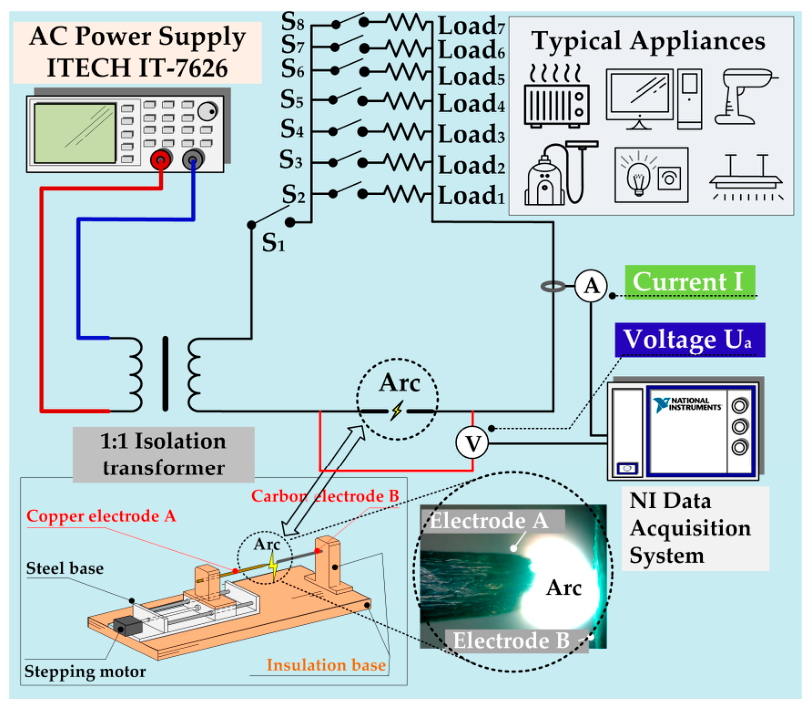
In this paper, starting from the statistical distribution characteristics of arc current signals, a novel series arc fault diagnosis method integrating differential sliding window higher-order cumulants and a stacked autoencoder is proposed. Specifically, an automated data acquisition platform is first constructed, where high-frequency current sensors are employed to collect current data from typical electrical loads under both normal and arc fault conditions to build the train and test datasets. A stacked autoencoder neural network is then developed, trained via a layer-wise approach with hyperparameter optimization, enabling accurate identification of series arc faults. Notably, the proposed algorithm features a lightweight architecture, is amenable to fixed-point quantization, and can be readily deployed on embedded platforms for real-time diagnosis, thereby providing a practical solution for arc fault protection in low-voltage distribution systems.

The novelty of this work lies in combining the differential sliding-window higher-order cumulant (HoC) feature extraction with the stacked autoencoder (SAE) diagnostic model—neither component is claimed as novel in isolation. Specifically, the differential sliding-window strategy applied to HoC features is introduced here for the first time, markedly improving discriminability for appliances with non-stationary currents (e.g., induction cookers) that conventional HoC methods handle poorly. In addition, integrating HoC feature vectors with SAE achieves a zero false alarm rate—a critical metric for practical AFCI deployment seldom reported in the prior works cited. Finally, the resulting lightweight architecture is directly amenable to fixed-point quantization and embedded deployment, bridging the gap between laboratory research and practical implementation.

2. Signal Acquisition and Analysis

2.1. Experimental Platform Setup

According to the Chinese standard GB 14287.4-2014, Electrical Fire Monitoring Systems—Part 4: Arc Fault Detection Devices [22], an arc fault acquisition experimental platform was constructed, as illustrated in Figure 1. The main equipment includes an adjustable point-contact arc generator with carbon and copper rods as electrodes, an NI PXI system, a programmable AC power supply (IT-7626, ITECH, Nanjing, China), seven typical test loads, an adjustable electronic load (IT-8616, ITECH, Nanjing, China), a 1:1 isolation transformer, and a current sensor (Keysight, N2783B, 100 MHz, 0.1 V/A, Keysight Technologies, Santa Rosa, CA, USA). The NI PXI system comprises a PXIe-1071 four-slot chassis, a PXIe-8133 controller, and a PXIe-5122 digitizer (National Instruments, Austin, TX, USA). The programmable AC power supply IT-7626 generates a rated voltage of 220 V at 50 Hz AC, with a 1:1 isolation transformer used to protect the IT-7626 from the arc fault current.

The PXIe-5122 digitizer is utilized to acquire the current signal in the circuit as well as the arc voltage across the arc. Arc voltage is also collected to readily verify whether an arc is generated in the circuit. The test loads consist of an adjustable electronic load (IT-8616) and seven typical electrical appliances, including a vacuum cleaner, an electric hand drill, a desktop computer, a fluorescent lamp, a dimmer, an electric heater, and an induction cooker, whose operating parameters are listed in

Table 1. Operating parameters of typical test appliances.

No.	Appliance	Rated Power (W)	Type
1	Electric heater	1200	Resistive
2	Fluorescent lamp	40	Capacitive
3	Dimmer	1000	Switching
4	Vacuum cleaner	1200	Inductive
5	Electric hand drill	500	Inductive
6	Desktop computer	450	Switching
7	Induction cooker	2200	Switching

.

2.2. Waveform Analysis of Current Signals of Typical Appliances

Figure 2a,c present the current time-domain waveforms of an electric heater and an induction cooker transitioning from normal operation to arc fault conditions, respectively, with the arc initiated at 0.02 s. All current data were processed using z-score normalization, resulting in a mean of 0 and a variance of 1. As can be observed, the current waveforms of the loads under normal operation exhibit sinusoidal patterns with significant variations depending on load type, yet the waveforms retain strict periodicity. During an arc fault, the current signal exhibits a “zero-current gap” phenomenon at zero-crossing points. The duration of the “zero-current gap” varies unpredictably across different loads, and abundant high-frequency components are generated at the zero-crossing points, and random high-frequency pulses associated with the arc appear during the remaining periods, disrupting the regular waveform pattern and eliminating its strict periodicity.

Figure 2b,d show the waveforms of the load currents for the electric heater and the induction cooker after filtering through a Butterworth high-pass digital filter with a cutoff frequency of 500 Hz. For the electric heater load, the filtered current exhibits pronounced arc pulse characteristics at the “zero-current gap,” with rich frequency components during the arc combustion phase. In contrast, for the induction cooker load, the envelope of the filtered current waveform is disrupted by the arc. The fault current signals exhibit super-Gaussian characteristics.

3. Statistical Distribution Characteristics and Higher-Order Cumulants of Arc Fault Currents and Normal Operating Currents Under Typical Appliances

3.1. Higher-Order Cumulants

Two important characteristics of a statistical distribution are central tendency and dispersion. For a normal distribution, once the mean and standard deviation are obtained, the distribution can be fully determined. However, if the data distribution is unknown, understanding the distributional shape requires not only measures of central tendency and dispersion but also skewness and kurtosis—collectively referred to as the shape of the distribution. Skewness and kurtosis were formalized by Karl Pearson in 1895 and 1905, respectively. These two measures can be derived from the higher-order central moments of the distribution [5].

Let $x$ be a random variable and let $k$ be a positive integer. If the expected value $E\left(x^k\right)$ exists, then $m_k=E\left(x^k\right)$ is referred to as the k-th raw moment (or moment about the origin) of the random variable $x$, and ${\mu }_k=E[{(x-E(x\left)\right)}^k]$ is referred to as the k-th central moment of the random variable $x$, as defined in Equations (1) and (2), respectively.

$$m_k=E\left(x^k\right)$$

(1)

$${\mu }_k=E[{(x-E(x\left)\right)}^k]$$

(2)

If the distribution function of the random variable $x$ is $F\left(x\right)$, then its characteristic function is defined as

$$\varphi \left(\omega \right)=E\left(e^{j\omega x}\right)={\int }_{-\infty }^{+\infty }{e}^{j\omega x}f\left(x\right)dx,$$

(3)

where $f\left(x\right)$ is the probability density function of the random variable $x$. If the random variable $x$ follows a normal distribution with mean $a$ and variance ${\sigma }^2$, i.e., $x~N(a,{\sigma }^2)$, then,

$$\varphi \left(\omega \right)=e^{j\omega a-{\displaystyle \frac{1}{2}}{\omega }^2{\sigma }^2}.$$

(4)

The natural logarithm of the characteristic function is defined as the second characteristic function. In the univariate case, the second characteristic function is given by

$$\psi \left(\omega \right)={lne}^{j\omega a-{\displaystyle \frac{1}{2}}{\omega }^2{\sigma }^2}=j\omega a-{\displaystyle \frac{1}{2}}{\omega }^2{\sigma }^2$$

(5)

Since the moments $m_k(1,2\cdots n)$ exist, the characteristic function and the second characteristic function of the random variable $x$ can be expanded in a Taylor series as

$$\varphi \left(\omega \right)=1+{\displaystyle \sum _{k=1}^n}{\displaystyle \frac{m_k}{k_{!}}}{\left(j\omega \right)}^k+O({\omega }^n)$$

(6)

$$\psi \left(\omega \right)=1+{\displaystyle \sum _{k=1}^n}{\displaystyle \frac{C_k}{k_{!}}}{\left(j\omega \right)}^k+O({\omega }^n)$$

(7)

In Equation (7), $C_k$ is referred to as the k-th cumulant of the random variable $x$. By comparing the coefficients of ${\left(j\omega \right)}^k(k=1,2\cdots n)$ between Equations (6) and (7), and assuming E(x) = 0, the relationship between the k-th cumulant and the k-th moment is given by

$$C_1=m_1=0$$

(8)

$$C_2=m_2-m_1^2=E\left[x^2\right]$$

(9)

$$C_3=m_3=E\left[x^3\right]$$

(10)

$$C_4=m_4-3m_2^2=E\left[x^4\right]-3{\left(E\right[x^2\left]\right)}^2$$

(11)

If the random variable x has a mean of 0 and a variance of 1, then the fourth cumulant is given by

$$C_4=m_4-3.$$

(12)

The noise-suppression capability of higher-order cumulants follows from the fact that, for any zero-mean Gaussian process, all cumulants of order three and above are identically zero. Consequently, for an observed signal composed of an arc fault current plus additive Gaussian noise, the fourth-order cumulant reflects only the non-Gaussian arc fault component, since the Gaussian noise is mathematically eliminated. Notably, the normal operating currents of household appliances also exhibit Gaussian-like statistical characteristics, and their contribution is likewise suppressed by the higher-order cumulant computation. This property ensures that the HoC features extracted in this study are not contaminated either by Gaussian background noise in the distribution grid or by the quasi-Gaussian interference from normal appliance operation, providing a robust statistical basis for arc fault detection.

3.2. Skewness and Kurtosis

Skewness measures the asymmetry of a data distribution relative to a normal distribution, while kurtosis measures the tailedness and peakedness of a data distribution relative to a normal distribution. Skewness is defined as the third standardized moment, and kurtosis is defined as the fourth standardized moment of the random variable x reduced by 3 [23,24].

According to Equations (10)–(12), as well as the definitions of kurtosis and skewness, if the signal has been processed by z-score normalization, then the raw moments of the signal are equal to its central moments. Specifically, the first cumulant equals zero, the second cumulant equals 1, the third cumulant equals the third moment, and the fourth cumulant equals the fourth moment minus 3. Consequently, the skewness of the signal corresponds to its third cumulant, and the kurtosis of the signal corresponds to its fourth cumulant. If the signal follows a Gaussian distribution, all cumulants above the second order are zero. Therefore, higher-order cumulants can effectively suppress the influence of Gaussian noise.

When an arc fault occurs, the current signal in the circuit exhibits super-Gaussian characteristics. Thus, skewness and kurtosis can be employed to analyze and characterize the statistical features of arc fault current signals.

3.3. Skewness and Kurtosis of Appliance Current Signals Under Normal and Arc Fault Conditions

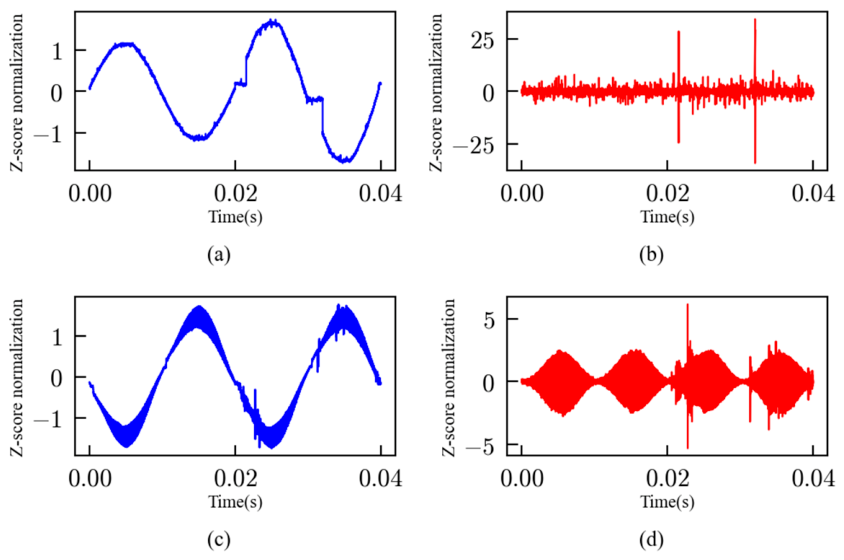
A current sensor was used to sample current data over one half-cycle period (10 ms) for seven typical appliances under both normal and arc fault conditions. The collected signals were filtered using a Butterworth high-pass digital filter with a cutoff frequency of 500 Hz to eliminate the fundamental frequency components, followed by z-score normalization. The skewness and kurtosis were then calculated for the seven typical appliances under both normal and arc fault conditions, as listed in

Table 2. Skewness and Kurtosis of Seven Typical Appliances Under Normal and Arc Fault Conditions.

No.	Appliance	State	Skewness	Kurtosis
1	Electric Heater	Normal	−0.32	32.66
		Arc fault	1.18	109.55
2	Vacuum Cleaner	Normal	0.11	29.82
		Arc fault	−21.84	3548.26
3	Desktop Computer	Normal	0.73	28.01
		Arc fault	0.06	46.38
4	Induction Cooker	Normal	−0.13	24.29
		Arc fault	0.18	47.85
5	Dimmer	Normal	0.11	15.81
		Arc fault	5.08	591.14
6	Electric Drill	Normal	0.11	7.81
		Arc fault	11.57	1005.64
7	Fluorescent Lamp	Normal	0.57	25.20
		Arc fault	1.65	60.52

.

The kurtosis values of all seven typical appliances under arc fault conditions are greater than those under normal conditions. Under normal conditions, the kurtosis values of the appliances are relatively close to each other, with the maximum being 32.66 for the electric heater. Under arc fault conditions, the minimum kurtosis is 46.38 for the desktop computer, whereas the maximum is 3548.26 for the vacuum cleaner. Under normal conditions, the skewness values of the appliances are very close to zero. Except for the desktop computer and the induction cooker, the skewness values of the remaining appliances under arc fault conditions can be clearly distinguished from those under normal conditions.

For the desktop computer and the induction cooker, the skewness and kurtosis values are relatively close between the two states. This is because the desktop computer is a switching-mode appliance, where the characteristic pulse currents of arc faults are randomly generated throughout the entire cycle with varying intensities and relatively low occurrence frequencies, thus having a minor impact on the statistical distribution of the current signal. For the induction cooker, since it exhibits rich harmonic components in the frequency band of 0~250 kHz under normal operating conditions, it already contains abundant frequency components. Observing the current waveform of the induction cooker, when an arc fault occurs, the high-frequency components generated by the arc are superimposed onto the existing frequency spectrum of the induction cooker. If the intensity of the arc characteristic signal is not sufficiently strong, its impact on the statistical distribution of the current sequence will also be small, resulting in weak discriminability in terms of both skewness and kurtosis.

To overcome the above issues, a differential sliding window method is proposed in this paper for processing the current data. The sampling rate of the current signal is 1 MS/s, and the time window length is set to 2 ms, so each time window contains 2000 data points. The window step size is set to 20, and 200 third cumulants and 200 fourth cumulants can be calculated for each half-cycle period (10 ms). Using this method, the skewness and kurtosis are calculated for the seven typical appliances under both normal and arc fault conditions. To make the abrupt signal changes more pronounced and mitigate the intensity differences between appliances, as well as to simplify the computation, the raw current signal is no longer processed by z-score normalization. Instead, a differential operation is directly applied by calculating the differences in skewness and kurtosis between consecutive windows. 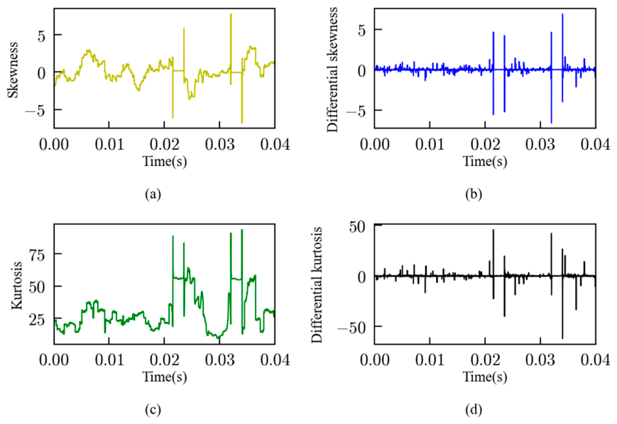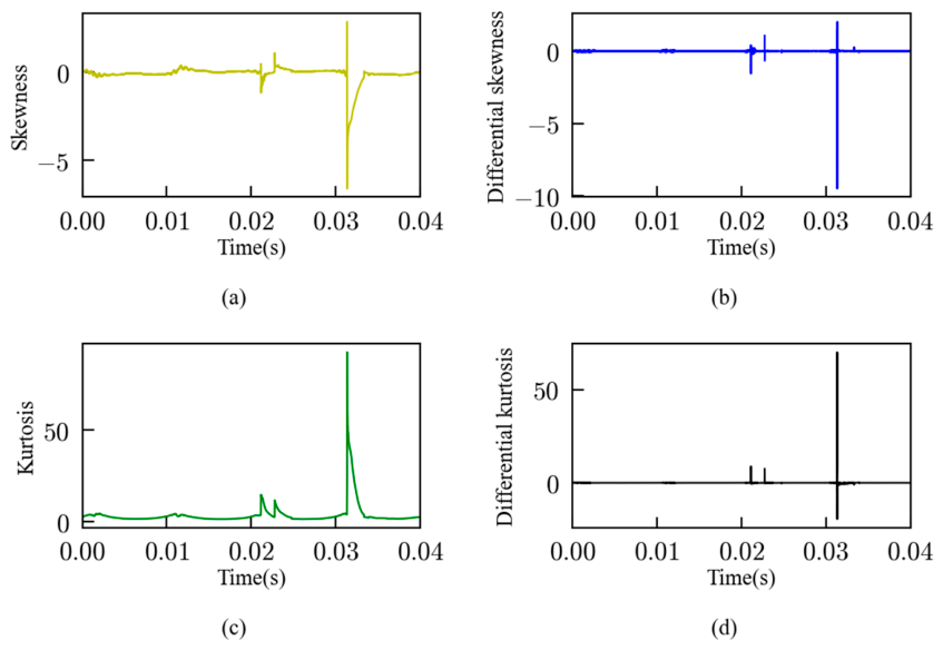Figure 3a,c and Figure 4a,c illustrate the variation trends of skewness and kurtosis for the electric heater and the induction cooker when an arc fault occurs, respectively.

When an arc fault occurs in the circuit, the fluctuation of the higher-order cumulants of the appliance current becomes more pronounced. The differential processing strategy stabilizes the higher-order cumulants such that they remain very close to zero during normal operation. This differential strategy can better distinguish arc fault conditions from normal conditions, as shown in Figure 3b,d and Figure 4b,d.

The variation in kurtosis is more pronounced under arc fault conditions, whereas it remains smooth under normal conditions. In theory, a fault threshold can be set based on the maximum kurtosis value under normal conditions, and arc fault identification can be achieved using a direct thresholding method—that is, an arc fault is detected when the kurtosis exceeds a predefined threshold. However, as shown in Table 2, the kurtosis values vary significantly across different appliances. Moreover, distribution systems often contain multiple types of appliances, and the wiring may be complex, with various types of noise and interference. Using a direct thresholding method for arc fault detection may lead to misclassification and reduce recognition accuracy.

4. Diagnosis of Arc Faults Using a Stacked Autoencoder with Higher-Order Cumulant Feature Vectors

Although the differential sliding window higher-order cumulant method can effectively characterize the statistical features of arc fault current signals, a direct thresholding approach is inadequate for practical applications involving multiple appliance types and complex interference environments. To address this limitation, a data-driven approach based on a stacked autoencoder is proposed in this section, which can automatically learn discriminative features from higher-order cumulant vectors and achieve robust arc fault diagnosis.

Specifically, the fourth cumulants within the differential sliding window are extracted to form feature vectors, which serve as input for feature learning. In this paper, a stacked autoencoder (SAE) is employed to extract deep representations from the HoC feature vectors, and an HoC-SAE arc fault diagnosis algorithm is proposed. The stacked autoencoder network, which possesses a symmetric architecture consisting of an encoding stage and a decoding stage, is designed using the PyTorch (Version 2.0.1) deep learning framework, adopting a layer-wise training strategy for network initialization. Training and testing are performed on a server equipped with four GPUs (NVIDIA GeForce GTX 1080Ti) and two CPUs (Intel Xeon E5-2678 v3).

4.1. Stacked Autoencoder

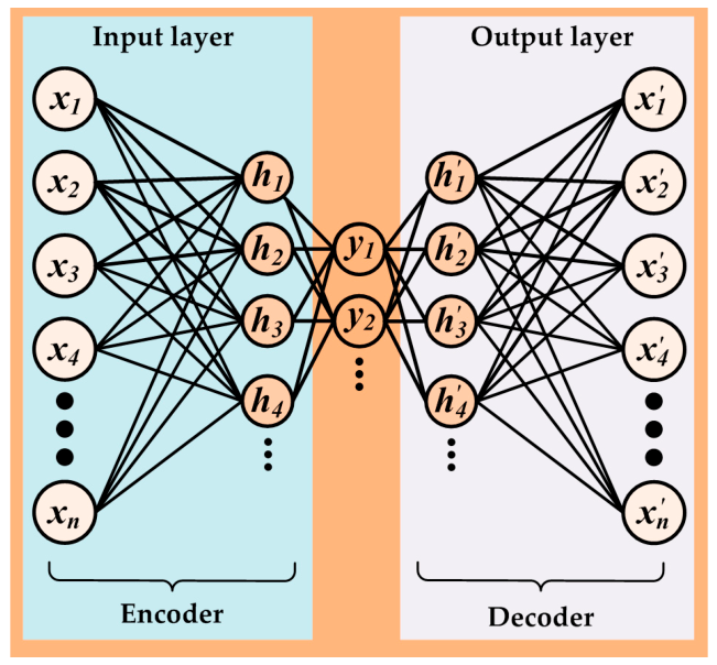
A stacked autoencoder is an artificial neural network that employs the backpropagation algorithm to make the output equal the input [25], featuring a symmetric “hourglass”-shaped architecture, as illustrated in Figure 5. A key characteristic is that the output dimension equals the input dimension—that is, the number of output neurons equals that of the input neurons, while the number of hidden layer neurons is smaller than that of the input neurons. The hidden layers can be either single or multiple. SAE performs unsupervised learning on sample data, with the objective of reconstructing the input using combinations of lower-level features, such that the error between the output neurons and the input neurons is minimized. The low-dimensional output of the hidden layer can faithfully reconstruct the high-dimensional input. This is an intuitive concept of dimensionality reduction, applicable to both linear and nonlinear transformations.

The stacked autoencoder (SAE) was selected as the diagnostic model for several reasons suited to the arc fault diagnosis scenario. First, SAE naturally functions as an anomaly detector, learning to reconstruct normal operational patterns from fault-free samples. When an arc fault signal is encountered, the reconstruction error increases because the fault pattern was not present during training. This reconstruction-error-based mechanism is conceptually aligned with distinguishing anomalous conditions from normal operation. Second, SAE performs unsupervised layer-wise pretraining, providing robust parameter initialization and avoiding vanishing gradient issues, a challenge when training deep networks on small-scale industrial datasets such as ours (2800 samples). Third, the symmetric encoder–decoder architecture encourages the network to preserve reconstruction-relevant features, providing implicit regularization that mitigates overfitting when training data are limited. Finally, the trained SAE produces a lightweight network (425 neurons, three hidden layers) deployable on resource-constrained embedded platforms, a practical requirement for arc fault circuit interrupters (AFCIs).

For training neural network models with multiple hidden layers, the backpropagation (BP) algorithm is commonly employed to update network parameters. However, careful initialization of the network parameters is required to prevent the network from falling into local optima. For neural networks with a large number of neurons and deep architectures, a poor choice of initial parameters can easily lead to vanishing or exploding gradients. SAE pre-training provides a simple yet effective approach to neural network parameter initialization [26].

4.2. Training and Testing of HoC-SAE

The SAE combined with HoC features of arc faults is employed for series arc fault identification. The main steps for training, testing, and validation of the HoC-SAE model are as follows:

• The train and test dataset are constructed. The absolute values of the fourth-order cumulant differentials are used as appliance feature vectors. The dataset consists of fourth-order cumulant feature vectors from the typical appliances and the electronic load IT-8616. Each typical appliance has 400 data samples, with each sample consisting of 200 fourth-order cumulant values. Among these, 200 samples are arc fault data, and the remaining 200 samples are normal operating condition data. The total dataset size is 2800 samples, of which 1400 samples are used for training the neural network, and 1000 samples constitute the validation dataset. The remaining 400 samples serve as the test dataset. To ensure generality, the electronic load IT-8616 is used to generate 300 additional current data samples with varying power factors, which are incorporated into the test dataset. In total, 700 samples constitute the test dataset, used to evaluate the trained SAE model.
• The stacked autoencoder network architecture is designed as follows: Each data sample consists of 200 fourth-order cumulant values; therefore, the number of input neurons is set to 200, and the number of output neurons is set to 2, corresponding to the two classification categories (normal and arc fault). SAE networks with 2, 3, and 4 hidden layers are configured, and their performance is evaluated;
• After each SAE layer is pre-trained in a layer-wise manner, a deep neural network with initialized parameters is constructed by connecting the output of each layer to the input of the next. The backpropagation method is then employed to fine-tune the weights and biases of the deep network. A SoftMax classifier is added as the final output layer, with the two output neurons denoted as $Y_0$ and $Y_1$ respectively;
• The cross-entropy loss function and the Adam optimizer [27] are employed for network training, with the learning rate set to 0.001 and the batch size set to 200. Based on the train loss and accuracy of networks with different architectures, the optimal number of network layers and the number of neurons per layer are selected.

The 300 electronic load samples in the test set were generated using a programmable AC/DC electronic load (IT-8616), comprising 150 arc fault and 150 normal samples under different power factor settings. Unlike the seven fixed household appliances used for training, each operating at a relatively fixed power factor, the IT-8616 can emulate various power factor conditions (e.g., lagging or leading), producing current waveforms whose shape and phase differ systematically from those of the training loads. This design serves as a generalization check: if the trained SAE model were overfitting to the specific current signatures associated with the training appliances’ native power factors, it would misclassify samples generated under unfamiliar power factor conditions. The test results in Section 5 confirm that the model maintains robust detection performance across all 300 IT-8616 samples (150 arc fault and 150 normal), demonstrating that it has learned the underlying arc fault features rather than load-specific power factor characteristics as the basis for discrimination.

4.3. Network Architecture and Hyperparameter Optimization

Following the steps described in Section 4.2, the higher-order cumulant method generates a feature vector of 200 dimensions from the current data of each half-cycle. Therefore, the number of neurons in the input layer of the SAE network is set to 200. First, a two-layer SAE network is constructed, and the effect of the number of neurons in the second hidden layer on the train and test results is evaluated. The optimal number of neurons in the second hidden layer is selected. The training results are listed in

Table 3. Accuracy of single hidden layer SAE.

Number of Hidden Neurons	Train Accuracy	Test Accuracy
5	92.3%	91.2%
10	95.4%	94.1%
15	94.7%	94.5%
20	93.5%	93.5%
25	94.1%	92.7%

.

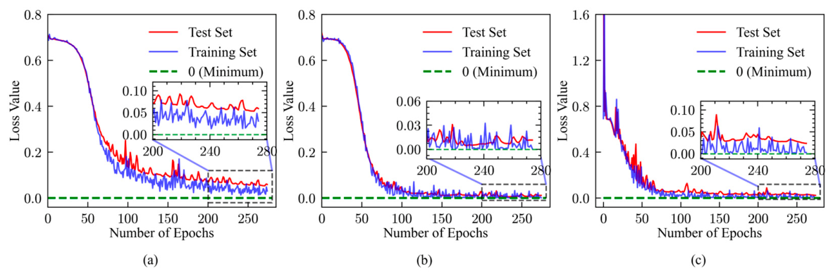
Both train and test accuracies of the single hidden layer SAE exceed 90%. The performance varies notably with different numbers of neurons. Increasing the number of neurons makes the network more difficult to train, leading to a decrease in train accuracy. With 10 hidden neurons, the train accuracy reaches 95.4% but the test accuracy is 94.1%. With 15 hidden neurons, the train accuracy drops slightly to 94.7%, while the test accuracy reaches 94.5%, the highest across all configurations, indicating the best generalization. Since generalization to unseen data is the primary objective, we select the neuron count based on test accuracy. The hidden layer immediately preceding the SoftMax classifier is therefore fixed at 15 neurons. Subsequently, the influence of multiple autoencoder layers on the performance of arc fault diagnosis is investigated. Networks with 3, 4, 5, and 6 layers are configured. The number of neurons per layer and the corresponding train and test accuracies are listed in

Table 4. Neurons per Layer and Train/Test Accuracies of Multi-Layer SAE.

Number of Hidden Layers	Number of Neurons per Hidden Layer	Test Accuracy	Test Accuracy
1	200-15-2	94.7%	94.5%
2	200-90-15-2	95.1%	94.7%
3	200-135-75-15-2	97.7%	96.4%
4	200-120-60-30-15-2	96.0%	93.8%

. The loss functions of the three network architectures are illustrated in Figure 6.

Multi-layer network architectures can learn features at different abstraction levels through training, i.e., capturing nonlinear relationships, thereby achieving better generalization performance. With fewer layers, the network may exhibit underfitting, as illustrated in Figure 6a. With fewer parameters to train, the loss function decreases slowly, resulting in a train loss lower than the test loss, and the loss function fails to converge. Conversely, for networks with more layers, as shown in Figure 6c, with a larger number of parameters, the loss function oscillates during the initial train phase. Moreover, this often leads to overfitting, where the train loss remains consistently lower than the test loss, with the train loss approaching zero.

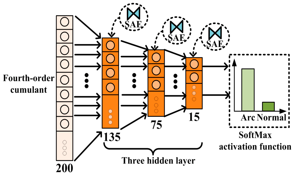
As shown in Figure 6b and Table 4, the three-hidden-layer SAE exhibits the best performance during both training and testing. The three-hidden-layer SAE architecture is illustrated in Figure 7. The final layer employs the SoftMax activation function, and the two output neurons are used to represent the normal state and the arc fault state, respectively.

4.4. Series Arc Fault Diagnosis Results Using HoC-SAE

The HoC-SAE diagnosis results and the corresponding confusion matrix are presented in

Table 5. Diagnosis Results of HoC-SAE and the Corresponding Confusion Matrix.

Appliance		Electric Heater	Vacuum Cleaner	Desktop Computer	Fluorescent Lamp
Predictions		60/60	49/50	60/60	56/60
Accuracy (%)		100	98.00	100	93.33
Appliance		Induction Cooker	Dimmer	Electric Drill	Electronic Load
Predictions		53/60	48/50	56/60	291/300
Accuracy (%)		96.67	88.33	96.00	97.00
	Predicted	Predicted: Normal		Predicted: Arc Fault
Actual		${\mathit{Y}}_{\mathbf{0}}=\mathbf{0},{\mathit{Y}}_{\mathbf{1}}=\mathbf{1}$		${\mathit{Y}}_0=1,{\mathit{Y}}_1=0$
Normal		350		0
Arc Fault		25		325
Overall Accuracy: 96.4% (675/700)

. The overall accuracy for arc fault identification is 96.4%, with a false alarm rate of 0% and a miss rate of 7.14%. Notably, the false alarm rate of this method is zero, indicating that the HoC-SAE method has excellent capability to suppress non-arc-fault signals from appliances.

5. Discussion

5.1. Algorithm Comparison

To compare the performance and diagnostic effectiveness of the proposed HoC-SAE algorithm for series arc faults, algorithms from references [16,28,29,30] are selected for comparison. These methods are compared in terms of their principles, sampling frequencies, applicable appliance types, and accuracy, as listed in

Table 6. Comparison of Attributes with Existing Methods.

Method	Principle	Sampling Frequency	Applicable Appliance Types	Accuracy
Ref. [16]	Deep neural network with Fourier, MFCC, and wavelet features as inputs	48 kHz	Resistive, switching (excluding capacitive and inductive) (ozone generator)	99.95%
Ref. [28]	LVQ-NN and PSO-SVM for load type detection and arc fault identification, respectively	5 kHz	Resistive, switching (excluding capacitive and inductive)	95.5%
Ref. [29]	Direct threshold method based on algebraic derivative of current	1 MHz	Resistive, reactive	Not mentioned
Ref. [30]	Sparse features of load types with fully connected network	25 kHz	Resistive, capacitive, switching, inductive	>94.3%
This Study	Higher-order cumulants and SAE	1 Mhz	Resistive, capacitive, switching, inductive	96.4%

. The appliance types and power ratings used by the algorithms in the table are the same as or similar to those used in this study.

The HoC-SAE diagnostic method employs the differential sliding window approach to extract the fourth-order cumulants of appliance currents, and then uses a stacked autoencoder network to identify series arc faults. This method achieves a zero false alarm rate.

Regarding the sampling rate, the HoC-SAE adopts a high sampling rate (1 MHz), the same as that of Reference [28] and significantly higher than those of References [16,28,30]. A higher sampling rate enables capturing more frequency information, but it also increases the hardware implementation cost. Therefore, a trade-off between the two aspects should be considered. Regarding the application scope, the HoC-SAE method can be applied to switching, inductive, purely resistive, and capacitive appliances, offering a broader range of applicability than References [16,28], which exclude capacitive and inductive appliances.

Regarding the detection accuracy, the HoC-SAE method achieves the second-highest accuracy, surpassed only by Reference [16]. Further refinement of hyperparameter optimization may yield even higher accuracy. However, it should be noted that Reference [16] employs an ozone generator to simulate series arc faults instead of using an arc generator recommended by relevant standards. The characteristics of the ozone generator differ significantly from those of real arc faults, which are unstable, intermittent, and random in nature. Whether it is appropriate to substitute real arc faults with an ozone generator remains debatable. Therefore, the accuracy reported in Reference [16] may not be representative. The accuracies of References [28,30] are both lower than that of the HoC-SAE method.

Although the current HoC-SAE system performs diagnosis locally on a single embedded device, with computationally lightweight HoC extraction analogous to FFT-based spectral analysis, future distributed arc fault monitoring networks could benefit from event-triggered communication strategies such as those proposed by Reference [31] to reduce transmission overhead while preserving diagnostic accuracy across networked AFCI nodes.

5.2. Analysis of Recognition Rates for Dimmer and Fluorescent Lamp

Although the overall accuracy of the HoC-SAE method is 96.4%, the recognition rates for the dimmer and fluorescent lamp are relatively low, at 88.33% and 93.33%, respectively. The dimmer, as a switching-type appliance, regulates power through phase control, which inherently introduces current discontinuities and transients during normal operation. These waveform distortions are similar to those caused by arc faults, making it difficult for the higher-order cumulant features to effectively distinguish between normal and fault conditions.

The fluorescent lamp, as a capacitive appliance, has an electronic ballast that generates high-frequency ripple currents, which may mask the frequency characteristics of arc faults. Moreover, the current distortion caused by arc faults in capacitive appliances is less pronounced than that in resistive appliances. In both cases, the normal operating currents of these appliances exhibit non-stationary characteristics, resulting in a smaller difference in higher-order cumulant features between normal and arc fault conditions.

In contrast, resistive appliances such as the electric heater achieve a recognition rate of 100%, as their steady current waveforms make the contrast between normal and fault conditions more distinguishable.

Notably, despite the relatively low recognition rates for these two appliances, the HoC-SAE method achieves a zero false alarm rate, indicating that no normal operating conditions are misidentified as arc faults. This represents a significant advantage, as avoiding false alarms is crucial for the practical application of arc fault detection.

5.3. Computational Efficiency and Implementation Challenges

The trained SAE network is a five-layer fully connected architecture with a 200-135-75-15-2 structure, totaling approximately 38,500 trainable parameters. This is substantially smaller than typical convolutional or recurrent architectures used in fault diagnosis tasks. The forward pass involves only matrix-vector multiplications and element-wise activation functions, with computational complexity linear in the number of layers and neurons. A single forward pass completes within a few milliseconds on a standard MCU, satisfying the real-time requirement of arc fault detection. Moreover, the lightweight architecture is amenable to fixed-point quantization, further reducing memory footprint and computational cost for embedded deployment on low-cost microcontrollers or FPGA platforms.

Nonetheless, several practical challenges remain. First, the current evaluation was conducted under controlled laboratory conditions using seven load types commonly found in residential environments; performance on industrial loads or mixed three-phase systems has not yet been verified. Second, while the architecture is conceptually suitable for fixed-point implementation, the actual quantization precision and its impact on detection performance require systematic experimental evaluation. Third, real-world deployment would need to account for factors such as electromagnetic interference, power supply stability, and long-term reliability of AFCI devices.

6. Conclusions

In this paper, to address the high false alarm rate problem in existing series arc fault diagnostic techniques based on line current, a series arc fault diagnosis method based on differential sliding window higher-order cumulants and SAE is proposed. The main conclusions are as follows:

• The current signals of low-voltage series arc faults exhibit super-Gaussian distribution characteristics. Calculating the fourth-order cumulant using the differential sliding window approach can effectively distinguish between the arc fault state and the normal operating state of appliances. The HoC-SAE network has a three-hidden-layer architecture with a total of 425 neurons, and can be readily ported to a general-purpose 32-bit microcontroller. However, the fourth-order cumulant computation in the differential sliding window method requires fourth-power calculations, which are computationally intensive for embedded implementation. Further research on simplifying the fourth-order cumulant computation is required.
• A dataset consisting of HoC feature vectors extracted from differential sliding windows is constructed. An SAE is adopted to construct the diagnostic model, and the performance of networks with different architectures is evaluated to obtain the optimal structure. The experimental results demonstrate that the HoC-SAE achieves an arc fault diagnosis accuracy of 96.4%, with a false alarm rate of 0%. Moreover, it exhibits excellent capability in suppressing non-arc-fault signals from appliances.
• Compared with existing methods, the HoC-SAE method achieves a zero false alarm rate and a broad range of applicability covering resistive, capacitive, switching, and inductive appliances. Although the recognition rates for the dimmer and fluorescent lamp are relatively low due to their non-stationary current characteristics, no normal operating conditions are misidentified as arc faults, which represents a significant advantage for the practical deployment of arc fault detection devices.