Modified Soft Margin Optimal Hyperplane Algorithm for Support Vector Machines Applied to Fault Patterns and Disease Diagnosis

Abstract

This paper introduces a modified soft margin optimal hyperplane (MSMOH) algorithm, which enhances the linear separating properties of support vector machines (SVMs) by placing higher penalties on large misclassification errors. This approach improves margin symmetry in both balanced and asymmetric data distributions. The research is divided into two main stages. The first stage evaluates MSMOH for synthetic data classification and its application in heart disease diagnosis. In a cross-validation setting with unknown data, MSMOH demonstrated superior average performance compared to the standard soft margin optimal hyperplane (SMOH). Performance metrics confirmed that MSMOH maximizes the margin and reduces the number of support vectors (SVs), thus improving classification performance, generalization, and computational efficiency. The second stage applies MSMOH as a novel synthesis algorithm to design a neural associative memory (NAM) based on a recurrent neural network (RNN). This NAM is used for fault diagnosis in fossil electric power plants. By promoting more symmetric decision boundaries, MSMOH increases the accurate convergence of 1024 possible input elements. The results show that MSMOH effectively designs the NAM, leading to better performance than other synthesis algorithms like perceptron, optimal hyperplane (OH), and SMOH. Specifically, MSMOH achieved the highest number of converged input elements $\left(1019\right)$ and the smallest number of elements converging to spurious memories $\left(5\right)$.

1. Introduction

Pattern classification uses software tools called classifiers to sort data into categories. For these classifiers to function effectively, they must be given carefully chosen input features that allow them to represent and differentiate between distinct classes within the data [1]. Among these tools, support vector machines (SVMs) stand out as a powerful supervised learning technique widely used across many applications due to their robust computational abilities in handling complex classification problems [2]. The operation of SVMs involves mapping input data into a high-dimensional feature space, where it becomes possible to construct a linear decision boundary. The specific characteristics of this boundary contribute to the model’s strong generalization capabilities. The foundational concept of SVMs is to identify an optimal separating hyperplane for cases where data is linearly separable. This approach is then adapted to non-separable data by introducing the concept of the soft margin hyperplane, which tolerates some misclassifications to find the best possible separation. SVMs have demonstrated exceptional performance in several key areas. For instance, in medical imaging they have a strong track record in breast cancer detection from images, where other methods are surpassing in accuracy [3]. For heart beat classification using electrocardiograms, SVMs integrated with artificial neural networks have also improved the performance [4]. In a broader comparison of machine learning algorithms, reference [5] found that SVMs consistently ranked among the best-performing methods. The study evaluated algorithms such as K-nearest neighbor, decision trees, and genetic algorithms. It concluded that both SVMs and long short-term memory networks delivered superior results in terms of both quality and quantity across different types of problems.

Although developed in the 1990s [6], SVMs remain a highly relevant and versatile tool for solving a wide range of modern problems. The continuous growth of artificial intelligence and advances in soft computing have led to new modifications and approaches that further improve SVM performance. Recent innovations have further enhanced the performance of SVMs. For example, a firefly algorithm-optimized SVM has been developed to achieve better classification accuracy than other methods [7]. In other applications, a hybrid model combining SVM with variable model decomposition has proven to be a useful and effective tool for making hydrological predictions in the context of climate change [8]. The integration of SVMs with meta-heuristic algorithms has become a popular method for improving their effectiveness. A notable example is a hybrid grey wolf optimizer combined with an improved sine cosine algorithm. This hybrid model enhances an SVM for classifying electroencephalography signals and achieves a very high classification rate [9]. In [10] a recent method called improved fuzzy least squares twin SVM enhances traditional SVMs for pattern classification. It improves performance by minimizing both structural and empirical risks, which leads to better generalization and faster processing speeds. A novel method called quantum SVM feature selection is introduced in [11] which combines quantum SVMs with multi-objective genetic algorithms. The purpose of this technique is to reduce the amount of data selecting most important features while also improving accuracy and overall performance.

For safety-critical systems like aero engines, chemical plants, and manufacturing, it is essential to ensure high levels of reliability and safety. This is particularly important because of the risk of process abnormalities and component faults. A key objective in these systems is to detect any faults as early as possible [12]. A fault can be defined as a change in a system’s properties or parameters that falls outside of its acceptable or standard operating conditions [13]. The classification of faults often depends on where they occur within a system (e.g., an overheating turbine engine or a cooling pump failure in a power plant). Consequently, a number of different approaches have been created to locate these faults. For instance, in [14] an artificial neural network based on a pattern recognition system is used to successfully detect a stator winding short circuit fault in a permanent magnet synchronous motor. In [15] authors developed a method to identify single fault patterns in power distribution networks with a convolutional neural network and fault pattern-based algorithm.

In this paper, the authors introduce a modified soft margin optimal hyperplane (MSMOH) to improve the linear separation capabilities of SVMs, and initial findings demonstrate that this modification maximizes the margin during hyperplane construction, which in turn reduces the number of support vectors (SVs) in comparison with conventional SMOH. Furthermore, the computational cost is significantly reduced. This ultimately leads to more effective classification for both synthetic data and heart disease diagnosis, where the statistical metrics (mean, standard deviation, and mean absolute generalization gap (MAGG)) during cross-validation indicate that MSMOH generalizes better than the SMOH. In the second stage, neural associative memory (NAM) based on a recurrent neural network (RNN) has been implemented for fault diagnosis in fossil electric power plants. A synthesis approach is developed to determine the weights and connection matrices of the NAM based on RNN using a new MSMOH algorithm which is a modification to the criterion usually utilized to determine the optimal hyperplane (OH) or soft margin optimal hyperplane (SMOH) in the synthesis of SVMs, reference [16]. The RNN is a type of Hopfield network that functions as an associative memory. Its purpose is to store desired patterns as stable memories. However, it is possible that undesirable patterns can appear as spurious memories, the number of which must be as small as possible for better efficacy of the NAM as described in [17,18,19,20]. This allows a stored pattern to be retrieved later, even when the initial input is only a partial or noisy version of that pattern. In practice, these memory patterns are typically represented using either bipolar or binary vectors which correspond to fault patterns that can appear in operation of a fossil electric plant. Once these fault patterns are stored, they can be retrieved when the input pattern contains enough information about that stored pattern. A convergence analysis is carried out using $2^{10}$ possible input elements $\left(1024\right)$ to the NAM using the new MSMOH with better results compared to other synthesis approaches such as perceptron, OH, and SMOH algorithms [17,18]. Specifically, MSMOH achieved the highest number of converged input elements $\left(1019\right)$ which converge to the stored fault pattern and the smallest number of possible input elements $\left(5\right)$ that converged to one of spurious memories (only 2).

This paper covers in Section 2 the materials and methods used, while Section 3 provides necessary mathematical background. This includes a detailed explanation of how to construct both the OH and SMOH for SVMs. It also introduces the principles of neural associative memory (NAM), a recurrent neural network model, and its associated training algorithms. In Section 4, MSMOH is introduced, along with the new objective functions developed to acquire corresponding parameters of the model. Section 5 presents classification results which are first presented with synthetic data and then with a heart disease database [21] which had been preprocessed previously where it is compared to conventional methods, where the margin maximization, the number of SVs, and the computational cost of the MSMOH shows better results compared with SMOH. Furthermore, metrics such as precision, sensitivity, specificity, accuracy, receiver operating characteristic (ROC) curve, and area under the curve (AUC) for classification results are obtained. Section 6 presents the NAM design with the MSMOH training for fault diagnosis in fossil electric power plants including convergence analysis, and finally, Section 7 and Section 8 present the discussion and conclusion of this paper.

2. Materials and Methods

This research is structured into two distinct stages. The first stage focuses on demonstrating the advantages of MSMOH in comparison to conventional SMOH. The second stage involves the training of a NAM, based on a recurrent neural network. This model incorporates the MSMOH developed in this study, and the reported results directly reflect this methodological approach.

1.

First Stage: Data Classification and Heart Disease Diagnosis with MSMOH Method.

• Following the description of MSMOH in Section 4, two different datasets are employed to illustrate the superiority of the new method. The first is a two-dimensional synthetic dataset with balanced distribution (symmetric), which allows for a visual comparison of the margin maximization offered by the constructed MSMOH versus SMOH.
• The heart disease database [21], sourced from the UCI repository, constitutes the second dataset with unbalanced data distribution (asymmetric). Prior to classification, this database underwent imputation, codification, and correlation analysis to optimize its representation. Subsequent analysis, encompassing performance metrics such as accuracy, precision, and confusion matrix, among others, are detailed in Section 5.

2.

Second Stage: Fault Pattern Diagnosis.

• Section 6 details the acquisition of fault patterns in fossil electric power plants, along with the procedures employed for codifying the measured patterns.
• Subsequent to the codification of fault patterns into bipolar vectors, a NAM is trained using the novel MSMOH synthesis to facilitate fault pattern diagnosis.
• An analysis of the results obtained from the trained NAM is presented, showcasing its significant advantages when compared to conventional training algorithms such as perceptron, OH, and SMOH.
• Furthermore, the convergence properties—including convergence, non-convergence, and spurious memories—were analyzed and compared for each training algorithm across all 1024 possible element combinations ($2^{10}$).

All analyses and methods described in this paper were performed using a Lenovo computer with an Intel(R) i7-10750H CPU, located in Guadalajara, Mexico with MATLAB R2020a installed (“MATLAB” is a registered trademark of the MathWorks, Inc., Natick, MA, USA). The heart disease database preprocessing, however, was completed in a Python 3.12 (“Python” is a registered trademark of the Python Software Foundation) environment using the pandas and scikit-learn [22] open source libraries in Google Colab.

3. Mathematical Preliminaries

This section begins by outlining the fundamental concepts of OH and SMOH, which are the basis of conventional SVM design [6]. It then proceeds to describe NAM equations [17,18,19,23] and its various training algorithms, which include perceptron, OH, and SMOH of SVM.

3.1. Optimal Hyperplane of SVM

SVMs are frequently used for two-class classification with a linear model of the following form:

$$\begin{array}{c}\hfill {\mathrm{{\rm Y}}}_i=W^T{X}_i+b\end{array}$$

(1)

where $X_i$ are the input vectors, W is a weight vector, and b is the bias term. The model is trained using a training set, O, which consist of M training examples. This set can be formally defined as follows:

$$\begin{array}{c}\hfill O=\{(X_1,y_1),(X_2,y_2),\dots ,(X_M,y_M)\}\end{array}$$

(2)

where the input pattern for the ith example is represented by $X_i\in R^n$, which is a vector with n elements. The corresponding class label for that example is $y_i\in \{-1,1\}$ to all M examples in the training set. In a linearly separable case, correct classification of data points are achieved by

$$\begin{array}{ccc}\hfill W^T{X}_i+b\ge 1,& for{y}_i=1& \end{array}$$

(3)

$$\begin{array}{ccc}\hfill W^T{X}_i+b\le -1,& for{y}_i=-1& \hfill \end{array}$$

(4)

These two conditions presented in Equations (3) and (4), which use the weight vector W and the bias term b, can be combined into a single inequality. The combined equality is as follows:

$$\begin{array}{cc}\hfill y_i(W^T{X}_i+b)\ge 1,& i=1,2,\dots ,M\end{array}$$

(5)

Moreover, the classification of new data points can be obtained through the evaluation of a sign function in the linear model (1):

$$\begin{array}{c}\hfill \widehat{y_i}=sign\left({\mathrm{{\rm Y}}}_i\right)\end{array}$$

(6)

The signed distance $G_i$ between $X_i$ and the OH is a measure of how far the point is from the decision boundary and on which side it lies. It is calculated using the following equation:

$$\begin{array}{c}\hfill G_i={\displaystyle \frac{(W^T{X}_i+b)}{\left|\right|W\left|\right|}}\end{array}$$

(7)

where $\left|\right|W\left|\right|$ is the Euclidean norm of the weight vector W, which normalizes the distance. To maximize the distance between classes, the norm of the weight vector, W, must be minimized. This can be achieved using the following function:

$$\begin{array}{c}\hfill F\left(W\right)={\displaystyle \frac{W^{T}W}{2}}\end{array}$$

(8)

Then, obtaining W and b for OH requires minimizing the function (8) considering the constraint in (5) which is equivalent to maximizing the margin, that is the distance between the hyperplane and the nearest data points [6]. The Lagrange multiplier functional $L(W,b,\mathrm{\Lambda })$ method can be used as follows [16,24]:

$$\begin{array}{c}\hfill L(W,b,\mathrm{\Lambda })={\displaystyle \frac{W^{T}W}{2}}-{\displaystyle \sum _{i=1}^M}{\alpha }_i[y_i(W^T{X}_i+b)-1]\end{array}$$

(9)

where the Lagrange multiplier vector $\mathrm{\Lambda }=({\alpha }_1,{\alpha }_2,\dots ,{\alpha }_M)$ is subject to ${\alpha }_i\ge 0$ for $i=1,2,\dots ,M$. To minimize (9) with respect to W, b, and $\mathrm{\Lambda }$, find the saddle point by minimizing it with respect to W and b and maximizing it with respect to the Lagrange multiplier. As described in [6,25], after getting the respective minimization, (9) can be transformed into the objective function $LL\left(\mathrm{\Lambda }\right)$ as follows:

$$\begin{array}{c}\hfill LL\left(\mathrm{\Lambda }\right)={\displaystyle \sum _{i=1}^M}{\alpha }_i-{\displaystyle \frac{{\mathrm{\Lambda }}^{T}D\mathrm{\Lambda }}{2}}\end{array}$$

(10)

with D as a positive semi-definite matrix [6], and $i=1,2,\dots ,M$, determined by the following equation:

$$\begin{array}{c}\hfill D={\displaystyle \sum _{i=1}^M}{\displaystyle \sum _{j=1}^M}{y}_i{y}_j{X}^{T}X\end{array}$$

(11)

$LL\left(\mathrm{\Lambda }\right)$ is only determined by (2) and the Lagrange multipliers; hence, minimizing (8), including restrictions (5), is simplified to maximizing $LL\left(\mathrm{\Lambda }\right)$ using Lagrange multipliers (${\alpha }_i$) satisfying the following equation:

$$\begin{array}{c}\hfill {\displaystyle \sum _{i=1}^M}{\alpha }_i{y}_i=0,\end{array}$$

(12)

$$\begin{array}{cc}\hfill {\alpha }_i& \ge 0\end{array}$$

(13)

Let $i=1,2,\dots ,M$. It is worth noting that (12) is obtained from the minimization of (9) in terms of b. If a solution to $LL\left(A\right)$ exists, it defines W and b for OH, and W may be expressed as a function of optimum Lagrange multipliers as follows:

$$\begin{array}{c}\hfill W={\displaystyle \sum _{i=1}^M}{\alpha }_i{y}_i{X}_i\end{array}$$

(14)

The OH has been used in several publications; however, its usefulness is restricted to linearly separable data [1].

3.2. Soft Margin Optimal Hyperplane

SMOH is introduced in [25,26] as an alternative to ease the linearly separable classes criterion. The restrictions are defined as follows:

$$\begin{array}{cc}\hfill y_i(W^T{X}_i+b)\ge 1-{\xi }_i,& i=1,2,\dots ,M\end{array}$$

(15)

$E={({\xi }_i,{\xi }_2,\dots {\xi }_M)}^T$, where ${\xi }_i\ge 0$ for $i=1,2,\dots ,M$. ${\xi }_i$ is also known as a “slack variable”, and there is one for each training data point. When ${\xi }_i=0$ there is no significant deviation, and the point is inside or in the margin boundary, while for other points, $\xi i= |y_i-{\mathrm{{\rm Y}}}_i|$. In Figure 1 the patterns affected with $\xi$ can be observed, where some are inside the margin, others are in the margin, and some are misclassified.

The search region for (15) is greater than that for (5), resulting in a better solution for optimization. The ${\xi }_i$ values represents deviations from SMOH and are minimized using the following criterion:

$$\begin{array}{cc}\hfill H=& {\displaystyle \sum _{i=1}^M}{\xi }_i^{\sigma }with\sigma >0\end{array}$$

(16)

In [25], it is additionally suggested to set $\sigma$ as “sufficiently small”. In [26], the following statement is presented: “For computational reasons, however, in this work it is considered the case $\sigma =1$. This scenario represents the smallest $\sigma >0$ that is still computationally simple”. For $\sigma <1$, the optimization problem may not be convex owing to computing complexity. $\sigma =1$ is the smallest number that guarantees computational feasibility, hence it is chosen for (16). Minimizing the $SMF\left(W\right)$ functional in Equation (17) with constraints (15) yields W and b for the SMOH.

$$\begin{array}{c}\hfill SMF\left(W\right)={\displaystyle \frac{W^{T}W}{2}}+C{\displaystyle \sum _{i=1}^M}{\xi }_i\end{array}$$

(17)

where the parameter $C\ge 0$ is a weighting factor that is set based on the specific problem. Its purpose is to balance the importance of the two main components in the equation. To find the solution of $SMF\left(W\right)$, Lagrange multipliers can be used. The solution to this problem is found by maximizing the Lagrange dual function, $SMLL\left(\mathrm{\Lambda }\right)$:

$$\begin{array}{c}\hfill SMLL\left(\mathrm{\Lambda }\right)={\displaystyle \sum _{i=1}^M}{\alpha }_i-{\displaystyle \frac{{\mathrm{\Lambda }}^{T}D\mathrm{\Lambda }}{2}}\end{array}$$

(18)

subject to the following:

$$\begin{array}{c}\hfill {\displaystyle \sum _{i=1}^M}{\alpha }_i{y}_i=0\end{array}$$

(19)

$$\begin{array}{c}\hfill 0\le {\alpha }_i\le C\end{array}$$

(20)

where D is a positive semi-definite matrix defined by (11). Maximizing (18), under constraints (19) and (20), is a simple quadratic programmatic (QP) [24]. The two dual maximization problems, OH (10) and SMOH (18), are extremely similar, with the main difference being the respective restrictions (13) and (20). After the Lagrange multipliers ${\alpha }_i$ are obtained, W can be obtained as depicted in Equation (14) considering corresponding restrictions. On the other hand, b can be obtained with the following equation:

$$\begin{array}{c}\hfill b={\displaystyle \frac{1}{S}}{\displaystyle \sum _{i\in S}}(y_i-W^T{X}_i)\end{array}$$

(21)

where $S=\{i:a_i>0\}$ represents the elements considered as SVs, and $y_i$ is considered as an example of the class.

3.3. Neural Associative Memory Based on Recurrent Neural Network

The primary function of a NAM is its ability to store patterns as stable memories. This allows a complete pattern to be retrieved, or recovered, even when the input is an incomplete or partial version of the stored pattern. In practice, these memory patterns are typically represented as bipolar vectors. The specific type of RNN used here is given by [17,18,19,23]:

$$\begin{array}{ccc}\hfill \dot{x}& =& -Ax+Tsat\left(x\right)+I\hfill \\ \hfill y& =& sat\left(x\right)\hfill \end{array}$$

(22)

where $x\in R^n$ is the state vector, $\dot{x}$ signifies the derivative of x with respect to time t, and $y\in D^n=\{x\in R^n:-1\le x_i\le 1,i=1,\dots ,n\}$ is the output vector, $A=diag[a_i,\dots ,a_n]$, where $a_i>0$ for $i=1,\dots ,n$. $T=\left[T_{ij}\right]\in R^n$ is the connection matrix, and $I=[I_1,\dots ,I_n]$ is the bias vector, and $sat\left(x\right)={[sat\left(x_1\right),\dots ,sat\left(x_n\right)]}^T$ denotes the activation function, where the following holds:

$$\begin{array}{c}\hfill sat\left(x_i\right)=\left\{\begin{array}{cc}1,\hfill & x_i>1\hfill \\ x_i,\hfill & -1\le x_i\le 1\hfill \\ -1,\hfill & x_i<-1\hfill \end{array}\right.\end{array}$$

(23)

The initial states of the system in Equation (22) are assumed to be within the range of $|x_i\left(0\right)|\le 1$ for all $i=1,\dots ,n$. It is important to note that this system is a variation of the analog Hopfield model, utilizing the saturation activation function, $sat\left(·\right)$. According to [19] a vector $\rho$ is considered a stable memory vector of the system if $\rho =sat\left(\beta \right)$ and if $\beta$ is an asymptotically stable equilibrium point of the system (22).

Lemma 1.

If $\rho \in {\beta }^n$ and if

$$\begin{array}{c}\hfill \beta =A^{-1}(T\rho +1)\in C\left(\rho \right),\end{array}$$

(24)

then $(\rho ,\beta )$ represents a pair of stable memory vectors and an asymptotically stable equilibrium point of (22). The proof of this lemma is available in [19].

Lemma 1 defines ${\beta }^n$ as a set of n-dimensional bipolar vectors ${\beta }^n=\{x\in R^n|x_i=1or-1,i=1,2,\dots ,n\}$. For $\rho ={[{\rho }_1,{\rho }_2,\dots ,{\rho }_n]}^T\in {\beta }^n$, define $C\left(\rho \right)=\{x\in R^n|x_i{\rho }_i>1,i=1,2,\dots ,n\}$. The following synthesis problem addresses the development of (22) for associative memories.

Synthesis problem: Given a set of m bipolar vectors ${\rho }^1,{\rho }^2,\dots ,{\rho }^m$ the synthesis problem is to find the system parameters $\{A,T,I\}$ such that the following two conditions are met:

1.

Each of the given vectors ${\rho }^1,{\rho }^2,\dots ,{\rho }^m$ becomes a stable memory vector for the system in Equation (22);

2.

The number of undesirable or ”spurious” memory vectors is minimized, and the basin of attraction for each of the desired memory vectors is maximized. This means that even a noisy or incomplete version of a desired vector can still successfully converge to the correct stored memory.

The first item of the synthesis problem can be guaranteed by choosing the $\{A,T,I\}$ such that every ${\rho }^i$ satisfies condition (24) of Lemma 1. The second item can be partly ensured by constraining the diagonal elements of the connection matrix. To solve this synthesis problem, A, T, and I from (24) need to be determinate considering $\rho ={\rho }^k$ and $k=1,2,\dots ,m$.

Considering this, the given condition in (24) can be equivalently written as follows:

$$\begin{array}{c}\hfill \left\{\begin{array}{cc}{T}_i{\rho }^k+I_i>a_i\hfill & if{\rho }_i^k=1\hfill \\ T_i{\rho }^k+I_i<-a_i\hfill & if{\rho }_i^k=-1\hfill \end{array}\right.\end{array}$$

(25)

where $T_i$ represents the $ith$ row of T. $I_i$ denotes the $ith$ element of I. $a_i$ is the $ith$ diagonal element of A, and ${\rho }_i^k$ is the $ith$ entry of ${\rho }^k$.

Training Algorithms for NAM

The NAM can be trained with different algorithms such as perceptron [19], OH [17], and SMOH [18] which have been employed to find the corresponding weights and bias to determine the best $A,T$ and I. These are some of the approaches that could be employed.

1.

Perceptron training algorithm

The perceptron has the following equation:

$$\begin{array}{c}\hfill Z=sign\left(Wu\right)\end{array}$$

(26)

where Z is the perceptron output, $u={[u_1,u_2,\dots ,u_n,1]}^T$ is the input vector, $W=[w_1,w_2,\dots ,w_n,\theta ]$ is the weight vector, and

$$\begin{array}{c}\hfill sign\left(ϵ\right)=\left\{\begin{array}{c}-1ϵ\ge 0\hfill \\ 1ϵ>0\hfill \end{array}\right.\end{array}$$

(27)

The perceptron training finds the weight vector W with the following steps considering $X_1$ and the patterns when $Z=1$ and $X_2$ when $Z=-1$.

(a)

Initialize the weight vector $W\left(l\right)$ for $l=0$.

(b)

For $l=0,1,2,\dots$

i.

If $W\left(l\right)u\left(l\right)\ge 0$ and $u\left(l\right)\in$$X_2$, then update

$W(l+1)=W\left(l\right)-\eta u\left(l\right)$;

ii.

If $W\left(l\right)u\left(l\right)<0$ and $u\left(l\right)\in$$X_1$, then update

$W(l+1)=W\left(l\right)+\eta u\left(l\right)$;

iii.

Otherwise, $W(l+1)=W\left(l\right)$, where $u\left(l\right)={\rho }^k$ for some $k,1\le k\le m$, and $\eta >0$ is the perceptron learning rate.

(c)

The training stops when no more updates for the weight vector W are needed.

The search of W weight values are presented as follows:

$$\begin{array}{c}\hfill W=[W_1^i,W_2^i,\dots ,W_n^i,W_{n+1}^i],i=1,2,\dots ,n.\end{array}$$

(28)

such that

$$\begin{array}{c}\hfill \left\{\begin{array}{cc}{W}^i{\rho }^{-k}\ge 0if\hfill & {\rho }_i^{-k}=1\hfill \\ W^i{\rho }^{-k}<0if\hfill & {\rho }_i^{-k}=-1\hfill \end{array}\right.\end{array}$$

(29)

for $k=1,2,\dots ,m$, and

$$\begin{array}{c}\hfill {\rho }^{-k}=\left[\begin{array}{c}{\rho }^k\\ \\ \dots \\ 1\end{array}\right]\end{array}$$

(30)

choose $A=diag[a_1,a_2,\dots ,a_n]$ with $a_i>0$. For $i,j=1,2,\dots ,n$ choose $T_{ij}=w_j^i$ if $i\ne j$. $T_{ii}=W_i^i+a_i{\mu }_i$ with $\mu >1$ and $I_i=W_{n+1}^i$.

2.

Optimal hyperplane algorithm

This training is based on the equations described in Section 3.1, where W values are obtained finding the Lagrange multipliers and the b value using the support vectors selected in the optimal hyperplane construction. However, the selection of $A,T$ and I are subject to the following equation:

$$\begin{array}{c}\hfill \left\{\begin{array}{cc}{W}^i{\rho }^{-k}+b\ge 1if\hfill & {\rho }_i^{-k}=1\hfill \\ W^i{\rho }^{-k}+b<-1if\hfill & {\rho }_i^{-k}=-1\hfill \end{array}\right.\end{array}$$

(31)

and the ${\rho }^{-k}$ vector is defined exactly as in (30). A notable distinction exists between the selection of NAM parameters and perceptron training regarding the determination of T and I. This process requires that $A=diag[a_1,a_2,\dots ,a_n]$ with $a_i>0$. For $i,j=1,2,\dots ,n$ choose $T_{ij}=w_j^i$ if $i\ne j$. $T_{ii}=W_i^i+a_i{\mu }_i-1$ with $\mu >1$ and $I_i=W_{n+1}^i+b_i$.

3.

Soft Margin Training Algorithm

Similar to the OH training, this training employs the equations presented in Section 3.2 for the search of optimal values to construct the SMOH. In this case, a hyperparameter C is introduced and must be correctly selected for the efficient training of the NAM. Once the weight vector is computed, the following condition must be accomplished

$$\begin{array}{c}\hfill \left\{\begin{array}{cc}{W}^i{\rho }^{-k}+b\ge 1+{\xi }_{i}if\hfill & {\rho }_i^{-k}=1\hfill \\ W^i{\rho }^{-k}+b<-1+{\xi }_{i}if\hfill & {\rho }_i^{-k}=-1\hfill \end{array}\right.\end{array}$$

(32)

where the ${\rho }^{-k}$ vector is again considered and defined as in (30), letting the NAM parameters be chosen with the same requirements as in the OH training algorithm where $A=diag[a_1,a_2,\dots ,a_n]$ with $a_i>0$. For $i,j=1,2,\dots ,n$ choose $T_{ij}=w_j^i$ if $i\ne j$. $T_{ii}=W_i^i+a_i{\mu }_i-1$ with $\mu >1$ and $I_i=W_{n+1}^i+b_i$.

Despite the selection of the $A,T$ and I parameters being similar to the OH training algorithm, the main difference is that obtaining the W and b parameters is based on the SMOH construction and hinge loss function. Further and deep analysis of the training algorithms for the NAM can be consulted in [17].

4. Proposed Soft Margin Optimal Hyperplane Modification

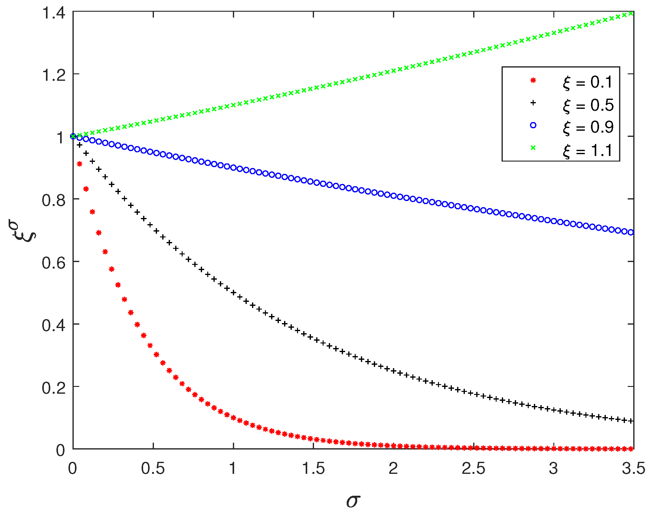
In this section, a new synthesis method for constructing a soft margin optimal hyperplane, MSOH, is introduced. This novel approach aims to improve upon the traditional methods for building the hyperplane in SVMs. The results of optimization are determined by the criterion used, which must be appropriate for the problem to be solved. Figure 2 shows how $\xi >0$ affects the function ${\xi }^{\sigma }$ for various positive values of $\sigma$. The effects of $\xi$ show that for criterion (16), when $\sigma <1$, the effect is similar and independent of $\xi$ values, and the function ${\xi }^{\sigma }$ converges to 1. Then, using (16), the optimization process considers small $\xi$ values (which do not create classification errors) in the same way, indicating that (16) is not an adequate criterion for classification.

To choose a more suitable optimization criterion for asymmetric data, it is a priority to minimize the effects of large $\xi$ values, as these lead to classification errors. This can be achieved by using a criterion that places a higher penalty on these larger errors, allowing for more fine-tuned adjustments to handle imbalanced datasets. The following criterion can be used for this purpose:

$$\begin{array}{c}\hfill K={\displaystyle \sum _{i=1}^M}{Q}_i{\xi }_i\end{array}$$

(33)

The weight values are now defined to be larger for significant $\xi$ values and smaller for minor ones, as follows:

$$\begin{array}{c}\hfill Q_i={\xi }_i^{p-1}\end{array}$$

(34)

for $i=1,2,\dots ,M$ and $p\ge 1$. Replacing (34) in (33), the following expression is obtained:

$$\begin{array}{c}\hfill K={\displaystyle \sum _{i=1}^M}{Q}_i{\xi }_i={\displaystyle \sum _{i=1}^M}{\xi }_i^{p-1}{\xi }_i={\displaystyle \sum _i^M}{\xi }_i^p\end{array}$$

(35)

with $p\ge 1$. From (35), the respective optimization process prioritizes large $\xi$ values, which produce classification errors.

In Figure 2, it is possible to see the differences in influence for large values of p (or $\sigma$ as described in the figure) and also for small increases in $\xi$ when p is large; hence, the proposed criterion (35) is very different from criterion (16) in [25]. In fact for (35) p should be big enough, instead of $\sigma$ being small enough as stated in (16). Then, $\sigma =1$ (as suggested in [1]) is the maximum value for criterion (16), and $p=1$ is the minimum one for criterion (35). Additionally, in [26] it is stated that due to computational efficiency, $\sigma =1$ is the only allowable value for (16). Due to similar considerations, $p\ge 1$ for (35). The case $p=1$ is a special instance where the hyperplane is constructed with the same SMOH objective function, as will be described later. The specific value of p depends on the problem being solved.

To define the MSMOH parameters, on the basis of criterion (35), it is required to minimize the following function, named $PSMF\left(W\right)$.

$$\begin{array}{cc}\hfill PSMF\left(W\right)={\displaystyle \frac{W^{T}W}{2}}+C{\displaystyle \sum _{i=1}^M}{\xi }_i^p& \end{array}$$

(36)

with $p\ge 1$ and $C>0$, where C is arbitrarily defined according to the problem to be solved. In fact, it is a weighting factor case as explained in (17). In order to guarantee convexity, p can be any value larger or equal to 1. Considering that $PSMF\left(W\right)$ is convex and (15) depends linearly on $W,b$ and ${\xi }_i$, then to solve this minimization problem no negative Lagrange multipliers ($\alpha$) can be applied [3], with the respective function formulated as follows:

$$\begin{array}{c}\hfill PSML(W,b,\mathrm{\Lambda })={\displaystyle \frac{W^{T}W}{2}}+C{\displaystyle \sum _{i=1}^M}{\xi }_i^p-{\displaystyle \sum _{i=1}^M}{\alpha }_i[y_i(W^T{X}_i+b)-1+{\xi }_i]-{\displaystyle \sum _{i=1}^M}{m}_i{\xi }_i\end{array}$$

(37)

where ${\alpha }_i$ are the Lagrange multipliers for (15), and $m_i$ are the ones for ${\xi }_i>0$. To solve (36), with constrains (15), the Lagrange multipliers can be applied, whose solution corresponds to the respective saddle point of (37), obtained by minimizing with respect to W, b, and ${\xi }_i$ and, simultaneously, maximizing with respect to the Lagrange multipliers.

The conditions for the minimum of $PSML$ (37) are as follows:

$$\begin{array}{cc}\hfill {\displaystyle \frac{\partial PSML}{\partial W}}=& W-{\displaystyle \sum _{i=1}^M}{\alpha }_i{y}_i{X}_i=0\end{array}$$

(38)

$$\begin{array}{cc}\hfill {\displaystyle \frac{\partial PSML}{\partial b}}=& -{\displaystyle \sum _{i=1}^M}{\alpha }_i{y}_i=0\end{array}$$

(39)

$$\begin{array}{cc}\hfill {\displaystyle \frac{\partial PSML}{\partial {\xi }_i}}=& pC{\xi }_i^{p-1}-{\alpha }_i-m_i=0\end{array}$$

(40)

From (38), W can be obtained as follows:

$$\begin{array}{cc}\hfill W=& {\displaystyle \sum _{i=1}^M}{\alpha }_i{y}_i{X}_i=0\end{array}$$

(41)

and from (39) the following constraint is defined:

$$\begin{array}{c}\hfill {\displaystyle \sum _{i=1}^M}{\alpha }_i{y}_i=0\end{array}$$

(42)

According to Kühn–Tucker conditions [6], the optimum point for ${\xi }_i\ne 0$ corresponds to $m_i=0$; then, from (40), ${\xi }_i$ is formulated as follows:

$$\begin{array}{c}\hfill {\xi }_i={{\displaystyle \frac{{\alpha }_i}{pC}}}^{\left({\displaystyle \frac{1}{p-1}}\right)}\end{array}$$

(43)

Substituting (41)–(43) in (37), and then transforming it, the following function is obtained:

$$\begin{array}{ccc}\hfill PSMLL\left(\mathrm{\Lambda }\right)& =& {\displaystyle \sum _{i=1}^M}{\alpha }_i-{\displaystyle \frac{{\mathrm{\Lambda }}^{T}D\mathrm{\Lambda }}{2}}+\left[{\displaystyle \frac{C}{{\left(pC\right)}^{\frac{p}{p-1}}}}-{{\displaystyle \frac{1}{pC}}}^{{\displaystyle \frac{1}{p-1}}}\right]{\displaystyle \sum _{i=1}^M}{\alpha }_i^{{\displaystyle \frac{p}{p-1}}}\hfill \\ \\ \hfill & =& {\displaystyle \sum _{i=1}^M}{\alpha }_i-{\displaystyle \frac{{\mathrm{\Lambda }}^{T}D\mathrm{\Lambda }}{2}}+C(1-p){\displaystyle \sum _{i=1}^M}{\left[{\displaystyle \frac{{\alpha }_i}{pC}}\right]}^{{\displaystyle \frac{p}{p-1}}}\hfill \end{array}$$

(44)

$PSMLL\left(\mathrm{\Lambda }\right)$ depends only on the training examples (2), Lagrange multipliers $\left({\alpha }_i\right)$, regulation parameter C and p being correctly selected. Hence, the minimization of (36) with constraint (15) is transformed to the maximization of $PSMLL\left(\mathrm{\Lambda }\right)$, with constraints (13) and (42). The values of the MSMOH parameters can be determined by means of (15), (41), and (43), and the optimal values of the Lagrange multipliers. In particular, the optimal value for b is calculated using the following equation:

$$\begin{array}{c}\hfill b={\displaystyle \frac{1}{S}}{\displaystyle \sum _{i\in S}}{\displaystyle \frac{{(1-\left(\frac{{\alpha }_i}{pC}\right))}^{\frac{1}{p-1}}}{y_i}}-W^T{X}_i\end{array}$$

(45)

where $S=\{i:0<{\displaystyle \frac{a_i}{C}}\le 1\}$ for $i=1,\dots ,M$ represents the elements considered as SVs, and $y_i$ is considered as the target value for the class label. The classification function is the same as described in Equation (6).

4.1. First Case of the Proposed Modification, p = 1

Consider the scenario wherein the parameter p approaches the value of 1 from the right-hand side. In order to prevent the final term of Equation (44) from becoming excessively large, it is necessary to consider the following function:

$$\begin{array}{cc}\hfill PSML{L}_1\left(\mathrm{\Lambda }\right)=& {\displaystyle \sum _{i=1}^M}{\alpha }_i-{\displaystyle \frac{{\mathrm{\Lambda }}^{T}D\mathrm{\Lambda }}{2}}\end{array}$$

(46)

Moreover, constraint (13) must be converted into constraint (20). Consequently, when $p=1$, the dual problem (44) associated with MSMOH simplifies to the dual problem (18) related to SMOH, incorporating constraints (19) and (20), as outlined in references [25,26].

4.2. Second Case of the Proposed Modification, p = 2

Considering $p=2$ in Equation (44), the function is solved as follows:

$$\begin{array}{cc}\hfill PSML{L}_2\left(\mathrm{\Lambda }\right)=& {\displaystyle \sum _{i=1}^M}{\alpha }_i-{\displaystyle \frac{{\mathrm{\Lambda }}^T(D+\left(\frac{1}{2C}\right)I)\mathrm{\Lambda }}{2}}\end{array}$$

(47)

where I is the identity matrix. The problem to maximize Equation (47) considering restriction (13) and (42) is a typical problem of QP.

4.3. Third Case of the Proposed Modification, p = 3

Considering $p=3$ in Equation (44), then the following holds:

$$\begin{array}{cc}\hfill PSML{L}_3\left(\mathrm{\Lambda }\right)=& {\displaystyle \sum _{i=1}^M}{\alpha }_i-{\displaystyle \frac{{\mathrm{\Lambda }}^{T}D\mathrm{\Lambda }}{2}}-2C{\displaystyle \sum _{i=1}^M}{\left[{\displaystyle \frac{{\alpha }_i}{3C}}\right]}^{{\displaystyle \frac{3}{2}}}\end{array}$$

(48)

4.4. Forth Case of the Proposed Modification, p = 4

In this case $p=4$ in function (44) resulting in the following:

$$\begin{array}{cc}\hfill PSML{L}_4\left(\mathrm{\Lambda }\right)=& {\displaystyle \sum _i^M}{\displaystyle \frac{{\alpha }_i-{\mathrm{\Lambda }}^{T}D\mathrm{\Lambda }}{2}}-3C{\displaystyle \sum _{i=1}^M}{\left[{\displaystyle \frac{{\alpha }_i}{4C}}\right]}^{{\displaystyle \frac{4}{3}}}\end{array}$$

(49)

Although new functions to be maximized under constraints (13) and (42) have been introduced, they cannot be resolved using QP. In instances where $p>2$, as established in (48) for $p=3$ and (49) for $p=4$, an alternative method must be employed to solve them. Moreover, the alternative method to solve the objective function of the proposed modification could search for a positive real optimal value of p with the condition of $p>1$.

5. Data Classification with MSMOH Synthesis for Support Vector Machines

This section details the implementation of the proposed MSMOH synthesis on synthetic data and a preprocessed heart disease database [21] (which underwent missing data imputation and codification). Section 5.1 and Section 5.2.2 compare the results from the new hyperplane synthesis with conventional SMOH. Subsequently, Section 5.2.3 employs cross-validation to illustrate the model’s advantages across varying input data. For this study, the search of the hyperparameter C has been optimized using the widely employed technique of grid search where the range of values in the grid is obtained by forming the search space with a series of logarithmically scaled intervals. Grid search explores all potential hyperparameter combinations inside the proposed space. For this study, the grid size and range are described in

Table 1. Grid Search space.

Hyperparameter	Range	Grid Size	Scale Type
C	$[{10}^{-7},{10}^{7.2}]$	700	Logarithmic

.

5.1. Classification of Synthetic Data with MSMOH

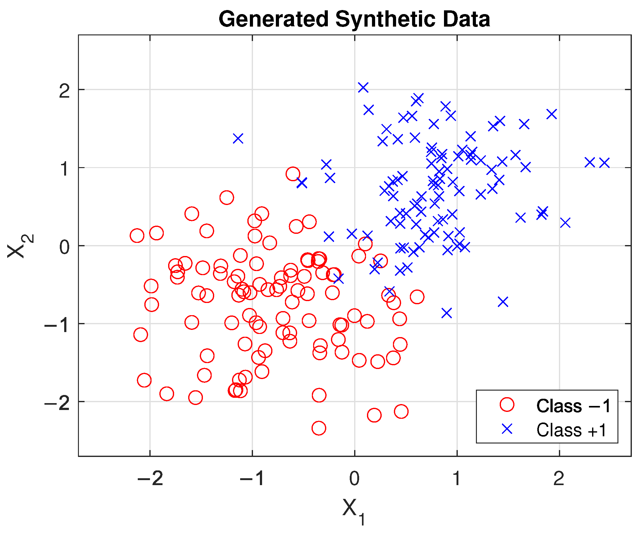
In a first stage, the proposed hyperplane construction is used to classify synthetic balanced data with features $X=\left[X_1{X}_2\right]$ and classes $Y=[-11]$, as depicted in Figure 3.

The data have been generated in MATLAB where the attributes contain 200 elements with 100 corresponding to class $-1$ and the other half to class 1. Moreover, the data are normalized with a mean of 0 and a standard deviation of 1, to a common scale to enhance SVM performance by preventing features with larger values from disproportionately influencing the model. For classification problems, the maximization of margin $\left(d\right)$ can be calculated with Equation (50) which is important in this section as will be presented in the classification results with the constructed hyperplane.

$$\begin{array}{cc}\hfill d=& {\displaystyle \frac{2}{\left|\right|W\left|\right|}}\end{array}$$

(50)

where $\left|\right|W\left|\right|$ is the norm of W.

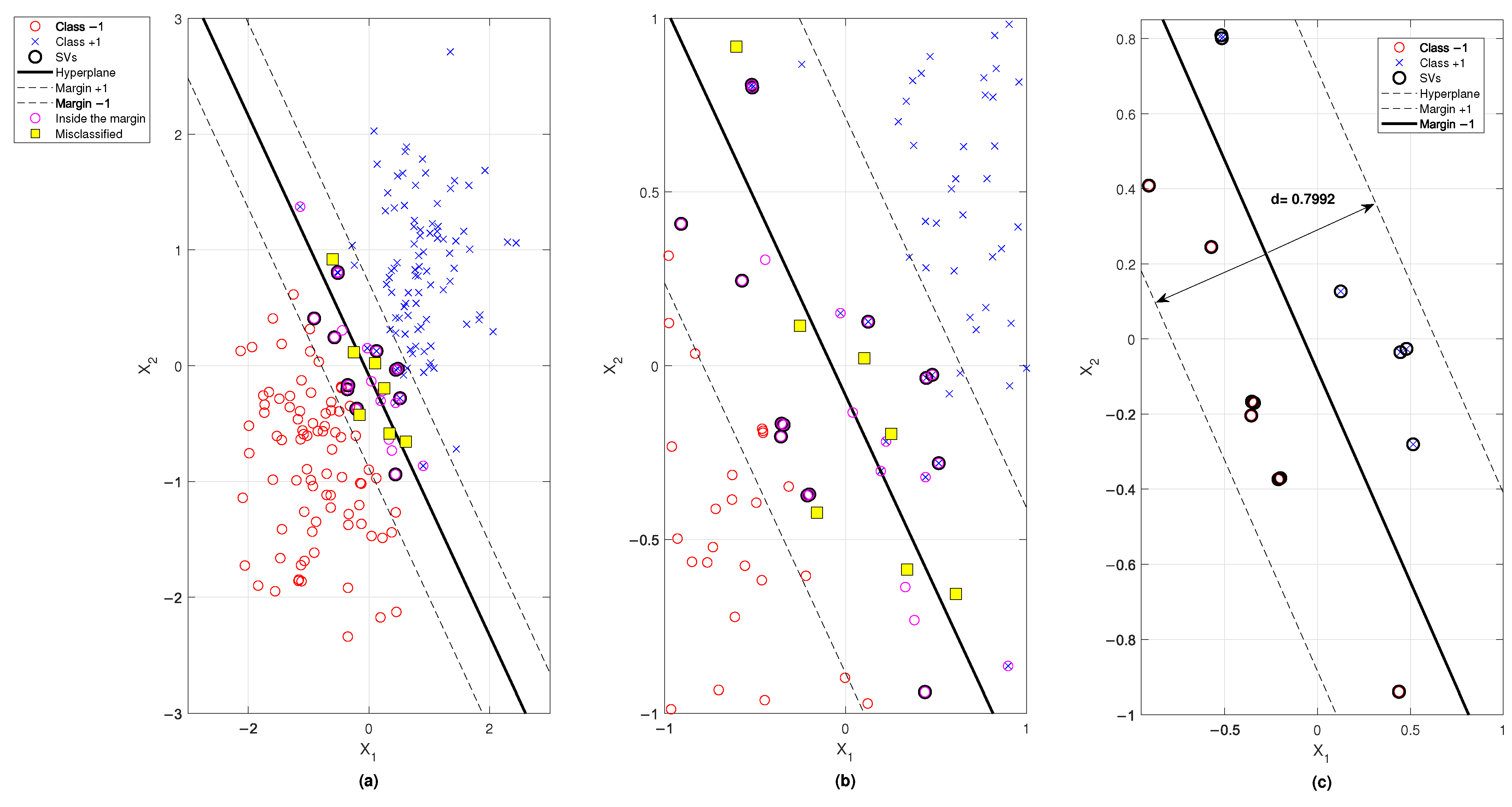
For simplicity, $p=2$ is used for the MSMOH, as this keeps the formulation as a QP problem. The regularization parameter, C, is set to $35.9441$ for both MSMOH and SMOH, a value determined through grid search and fine adjustment. As presented in

Table 2. Classification metrics for MSMOH and SMOH methods.

Method	Accuracy	Sensitivity	Specificity	Precision	SVs
MSMOH	$96.50\%$	$97.00\%$	$96.00\%$	$96.04\%$	14
SMOH	$96.00\%$	$96.00\%$	$96.00\%$	$96.00\%$	171

, the MSMOH classifies data with superior performance metrics compared to SMOH, specifically for accuracy, sensitivity, and precision. This enables the classifier to accurately detect true positive cases in the case of sensitivity. However, precision shows how frequently the model’s positive predictions are accurate, and the more precise the model is, the fewer false positives it produces. Finally, accuracy quantifies the percentage of accurate predictions the SVM makes out of all model predictions. Moreover, construction of the hyperplane is illustrated in Figure 4a,b where the number of SVs is illustrated with a bold contour, and the constructed hyperplane and the misclassified elements, among others, are described such that it is demonstrated how maximization of the hyperplane with MSMOH synthesis could be accomplished with a fewer number of SVs as presented in Figure 4c where $d=0.7992$. On the other hand, with the SMOH results, classification performance is good but with a dependency on the use of a great amount of SVs, contrarily to the MSMOH as presented in Table 2.

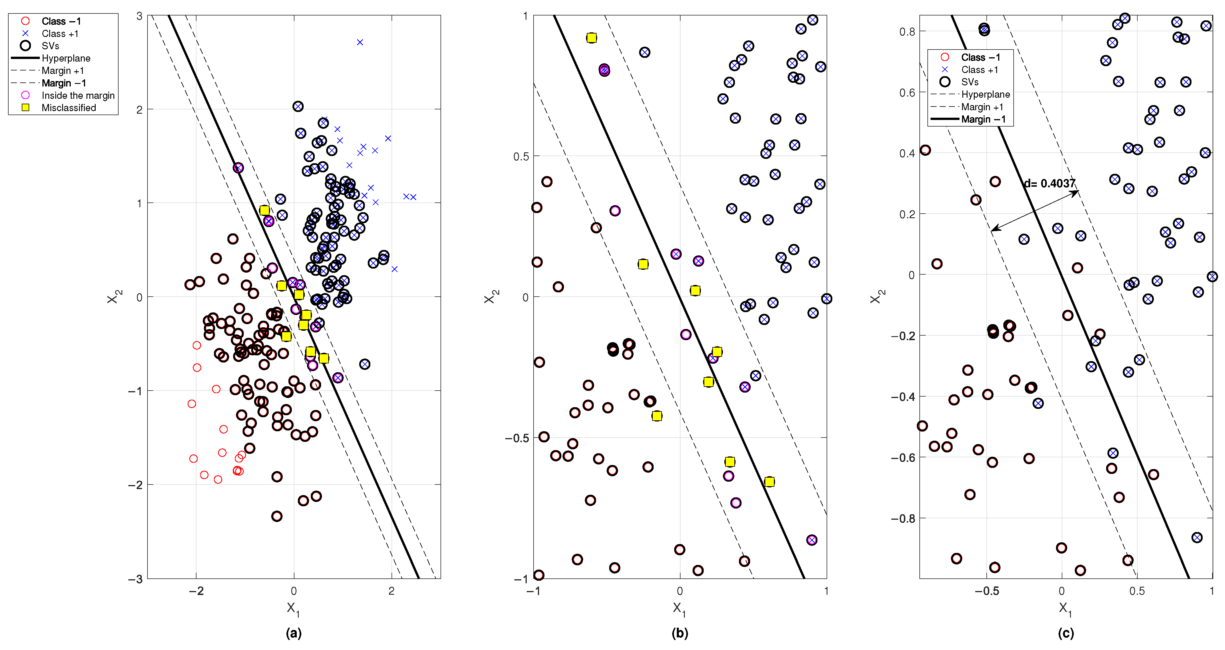
Furthermore, maximization of the margin is lower compared to the one obtained with new synthesis giving a value $d=0.4037$. Classification and maximization of margin with SMOH is presented in Figure 5a, b, and c respectively. Although the MSMOH performance showed a significant improvement in the classification task, using real-world data is necessary to increase the reliability of the SVM model.

Average computational cost has been calculated using the “tic” and “toc” function of MATLAB for the training of the SVM with MSMOH and SMOH over a different instances. The results are presented in

Table 3. Average computational cost for MSMOH and SMOH methods.

Method	1 Time	10 Times	100 Times	500 Times	1000 Times
MSMOH	$0.6682\mathrm{s}$	$0.0808\mathrm{s}$	$0.0144\mathrm{s}$	$0.0080\mathrm{s}$	$0.0073\mathrm{s}$
SMOH	$0.6883\mathrm{s}$	$0.0832\mathrm{s}$	$0.0159\mathrm{s}$	$0.0094\mathrm{s}$	$0.0087\mathrm{s}$

where the MSMOH has a faster response in training which reflects a lower computational cost.

5.2. Heart Diseases Diagnosis with MSMOH

Despite the improved classification performance of MSMOH, real-world data is crucial to fully demonstrate its advantages. For this purpose, a database for diagnosing heart diseases has been selected. However, this database contained significant missing data and categorical information. Consequently, it was preprocessed to achieve the best attribute representation for detecting heart disease in patients. The preprocessing steps are detailed in Section 5.2.1. The heart disease diagnosis using SVM-MSMOH is presented in Section 5.2.2, and the same SVM with MSMOH, utilizing cross-validation, is discussed in Section 5.2.3.

5.2.1. UCI Heart Disease Database Preprocessing

This database comprises information on 920 patients, each with 16 diagnostic attributes related to heart problems. Of these, 509 patients are labeled with heart disease and 411 are not.

Table 4. UCI heart disease database attributes.

Attribute	Description	Non-Null Count 1	Data Type 1
ID	Unique for each patient	920 non-null	int64
Age	Age of patients in years	920 non-null	int64
Origin	Place of study	920 non-null	object
Sex	Male/Female	920 non-null	object
cp	Chest Pain Type	920 non-null	object
trestbps	Resting Blood Pressure	861 non-null	float64
chol	Serum Cholesterol (in mg/dL)	890 non-null	float4
fbs	Indicates if Fasting blood sugar $>120$ mg/dL	830 non-null	object
restecg	resting electrocardiographic results (normal, Stt abnormality, lv hypertrophy)	918 non-null	object
thalch	Maximum Heart rate achieved	868 non-null	float64
exang	Exercise-induced angina (True/False)	865 non-null	object
oldpeak	ST depression induced by exercise relative to test	858 non-null	float64
slope	The slope of the peak exercise ST segment	611 non-null	object
ca	Number of major vessels (0–3) colored by fluoroscopy	309 non-null	float64
thal	Thalassemia (normal; fixed defect; reversible defect)	434 non-null	object
num	The predicted attribute (0 = heart disease; 1, 2, 3, 4 = Stages of heart disease)	920 non-null	int64

¹ Analyzed with Pandas and sci-kit learn open-source library.

presents these data attributes, including the amount of data available for each. Data treatment, considering visualization and implementation, is performed using scikit-learn and pandas libraries. Initial step involved encoding data using label encoding method. This technique transforms categorical data into a numerical format, making it compatible with machine learning methods like SVM. Several encoding techniques were considered, including one-hot encoding (for binary representation), label encoding (assigning unique ordinal numerical values), hashing (mapping categories to numerical values for dimensionality reduction), and target encoding (replacing categories with the mean or mode of the label).

For this study, label encoding has been specifically selected because the original data includes various attributes that are not suitable for binary representation, unlike what one-hot encoding offers. Examples of attributes where this coding was applied include “Chest pain type,” “dataset” (now referred to as “Origin”), “sex,” and “ST-segment slope type.” Original description of attribute and resulting encoding are illustrated in

Table 5. Data information.

Sex	Dataset	cp	restecg	exang
Male	Cleveland	typical angina	lv hypertrophy	False
Male	Cleveland	asymptomatic	lv hypertrophy	True
Male	Cleveland	asymptomatic	lv hypertrophy	True
Male	Cleveland	non-anginal	normal	False
Female	Cleveland	atypical angina	lv hypertrophy	False

and

Table 6. Codified data information.

Sex	Dataset	cp	restecg	exang
1	0	3	1	0
1	0	0	1	1
1	0	0	1	1
1	0	2	2	0
0	0	1	1	0

. For incomplete data, an imputation strategy has been applied to replace missing values with reasonable estimates derived from the dataset itself. Specifically, continuous variables such as blood pressure, cholesterol, and ST-segment depression have been imputed using the mean, as this approach preserves the central tendency of physiological measurements without introducing significant bias. Conversely, categorical and discrete variables such as the number of colored blood vessels and exercise-induced angina have been imputed using the mode, since replacing missing values with the most frequent category maintains the natural distribution of these attributes.

This combined mean–mode strategy prevents information loss that would result from case deletion, ensures consistency across the dataset, and supports robust model training, thereby enhancing the generalization capacity of the proposed methodology. As a result, the dataset is now complete, as shown in

Table 7. Completed data using imputation technique.

Attribute	Description	Non-Null Count 1	Data Type 1
ID	Unique for each patient	920 non-null	int64
Age	Age of patients in years	920 non-null	int64
Origin	Place of study (0–3)	920 non-null	int64
Sex	Male/Female	920 non-null	int64
cp	Chest Pain Type	920 non-null	int64
trestbps	Resting Blood Pressure	920 non-null	float64
chol	Serum Cholesterol (in mg/dL)	920 non-null	float4
fbs	Indicates if Fasting blood sugar $>120$ mg/dL	920 non-null	int64
restecg	Resting electrocardiographic results (normal, Stt abnormality, lv hypertrophy)	920 non-null	int64
thalch	Maximum Heart rate achieved	920 non-null	float64
exang	Exercise-induced angina (True/False)	920 non-null	int64
oldpeak	ST depression induced by exercise relative to test	920 non-null	float64
slope	The slope of the peak exercise ST segment	920 non-null	int64
ca	Number of major vessels (0–3) colored by fluoroscopy	920 non-null	float64
thal	Thalassemia (normal; fixed defect; reversible defect)	920 non-null	int64
num2	The predicted attribute (−1 = no heart disease; 1 = Heart disease)	920 non-null	int64

¹ Analyzed with pandas and sci-kit learn open-source library. ² For simplicity, the “num” attribute was converted into a bipolar vector to indicate the presence or absence of heart disease where 509 patients are from class 1, and 411 are from class −1.

.

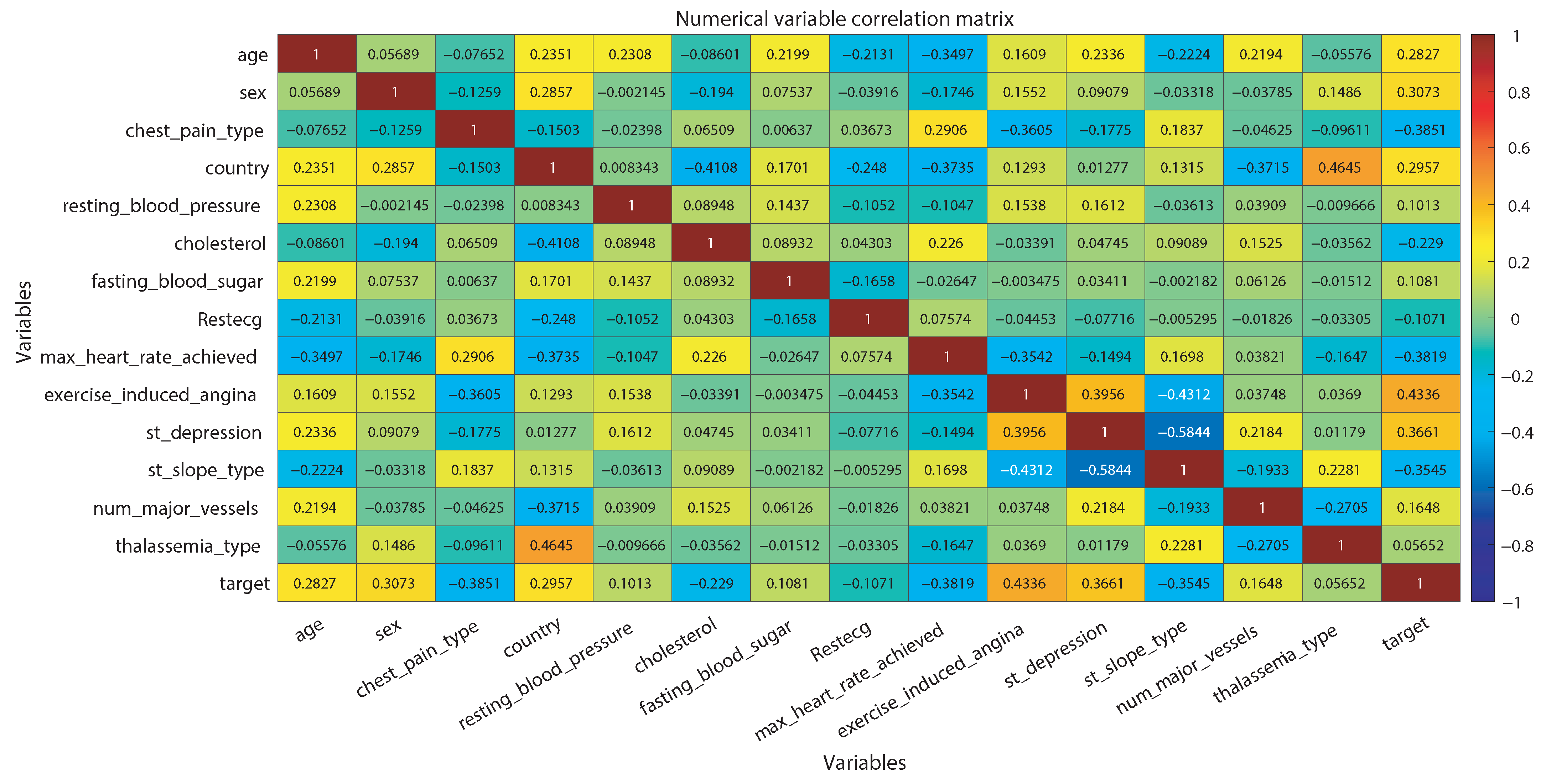
Finally, a correlation analysis has been conducted in MATLAB^® to find the attributes that are important and significantly represent the patients characteristics. From this, a correlation threshold $>\left|0.15\right|$ was selected to find attributes that could better work for diagnosis of heart diseases. In Figure 6 the obtained correlation results are presented, and the 10 selected attributes are as follows: exang, cp, thalch, oldpeak, slope, Sex, country, Age, chol, and ca.

5.2.2. Heart Disease Diagnosis with SVM-MSMOH Classification

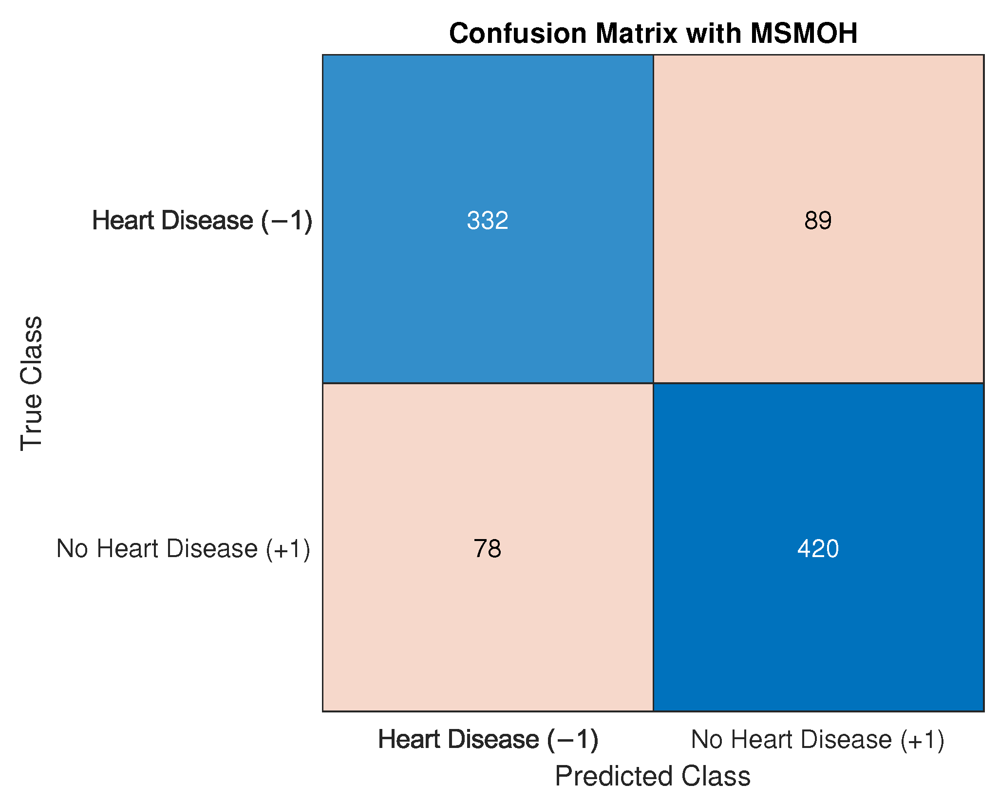
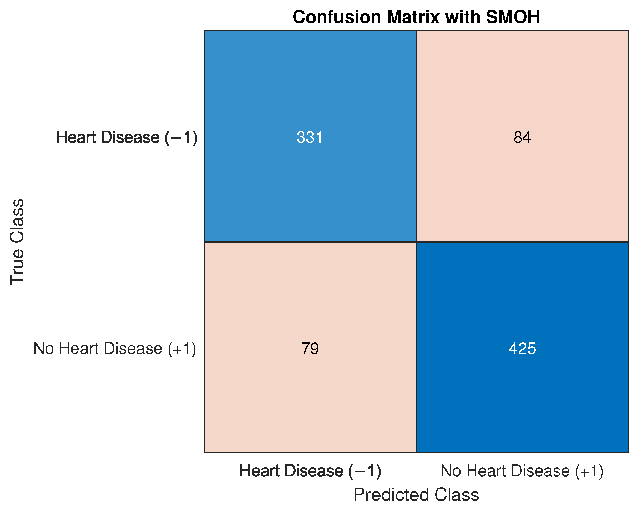
Once the database has been preprocessed and is ready for use, the classification task is carried out. In this initial case, all elements of the database are employed to diagnose heart disease. Additionally, more metrics of performance are introduced such as a confusion matrix and F1-score which will help to measure the performance with the imbalanced classes of the database. In this case, for the MSMOH, $p=2$, and the regularization term C is set to 83,168.5597 for both MSMOH and SMOH; this value was again determined through a grid search (Table 1) and fine adjustment. Performance results of the SVM classification, presented and compared in

Table 8. Heart disease classification metrics with SVM-MSMOH using all data.

Method	Accuracy	Sensitivity	Specificity	Precision	F1-Score	Support Vectors	Margin
MSMOH	$81.8280\%$	$82.5147\%$	$80.9756\%$	$84.3373\%$	$0.8341$	327	$3.8909$
SMOH	$82.2633\%$	$83.4970\%$	$80.7317\%$	$84.3253\%$	$0.8390$	403	$1.7646$

, reveal that SMOH outperforms MSMOH in accuracy, sensitivity, and F1-score when using the entire dataset. However, the results also show that MSMOH has better precision and specificity than SMOH. Furthermore, MSMOH offers similar classification performance while using fewer support vectors and a wider margin for hyperplane construction. This suggests that MSMOH is a simpler model. It may also generalize better to new, unseen data. The confusion matrices for MSMOH and SMOH are presented in Figure 7 and Figure 8, respectively.

An interpretation of these results suggests that SMOH is marginally more effective in terms of overall accuracy and its ability to correctly identify true positive cases (sensitivity). In contrast, MSMOH demonstrates superior performance in correctly identifying healthy patients (specificity) and in the reliability of its positive predictions (precision). Even though the performance of both classifiers is similar, their ability to generalize to new data has not been entirely tested. To provide a more robust evaluation, the next section explores their classification performance using cross-validation to validate models on unseen data.

5.2.3. Heart Disease Diagnosis with Cross-Validation

Previously, the SVM-SMOH and SVM-MSMOH models are evaluated using a full-sample training approach. To obtain a more robust and reliable estimate of the generalization performance of the models and to assess the advantages of the proposed modification, a k-fold cross-validation scheme is subsequently implemented. Cross-validation is a technique used in machine learning to assess how well a model generalizes to unseen data helping to prevent overfitting, where a model performs well on training data but poorly on new data. The chosen technique is selected due to the moderate size of the dataset.

Cross-validation is performed using five folds, partitioning data into a training set of 735 elements and a validation set of 184, with performance metrics presented in

Table 9. Heart disease classification training metrics with SVM-MSMOH in cross-validation with 5 folds.

Fold	Accuracy in Training	Sensitivity in Training	Specificity in Training	Precision in Training	F1-Score in Training	SVs	Margin
1	$82.2010\%$	$83.0918\%$	$81.0559\%$	$84.9383\%$	$0.8400$	261	3.7324
2	$81.3605\%$	$83.4135\%$	$78.6834\%$	$83.6145\%$	$0.8351$	270	3.9522
3	$81.7687\%$	$82.1159\%$	$81.3609\%$	$83.8046\%$	$0.8295$	281	3.9357
4	$82.4489\%$	$82.4121\%$	$82.4926\%$	$84.7545\%$	$0.8356$	265	3.7586
5	$82.1768\%$	$83.9416\%$	$79.9383\%$	$84.1463\%$	$0.8404$	251	3.8735
Mean	81.9911%	82.9949%	80.7062%	84.2516%	0.8361	265.6	3.8504
Standard Deviation	0.4287%	0.7404%	1.4511%	0.5790%	0.0044	11.0815	0.1006

and

Table 10. Heart disease classification test metrics with SVM-MSMOH in cross-validation with 5 folds.

Fold	Accuracy in Test	Sensitivity in Test	Specificity in Test	Precision in Test	F1-Score in Test
1	$79.7814\%$	$80.0000\%$	$79.5455\%$	$80.8511\%$	$0.8042$
2	$83.6956\%$	$83.8710\%$	$83.5165\%$	$83.8710\%$	$0.8387$
3	$81.5217\%$	$83.0357\%$	$79.1667\%$	$86.1111\%$	$0.8454$
4	$81.5217\%$	$81.9820\%$	$80.8219\%$	$86.6667\%$	$0.8425$
5	$81.5217\%$	$81.6327\%$	$81.3953\%$	$83.3333\%$	$0.8247$
Mean	81.6084%	82.1042%	80.8891%	84.1666%	0.8311
Standard Deviation	1.3889%	1.4709%	1.7274%	2.3348%	0.0170

. Table 9 presents the training results for each fold, detailing metrics such as accuracy, sensitivity, specificity, precision, and F1-score, in addition to the number of SVs and the margin. Moreover, metrics such as the mean and standard deviation are included. In test and training, the standard deviation illustrates how consistent the model is throughout the folds.

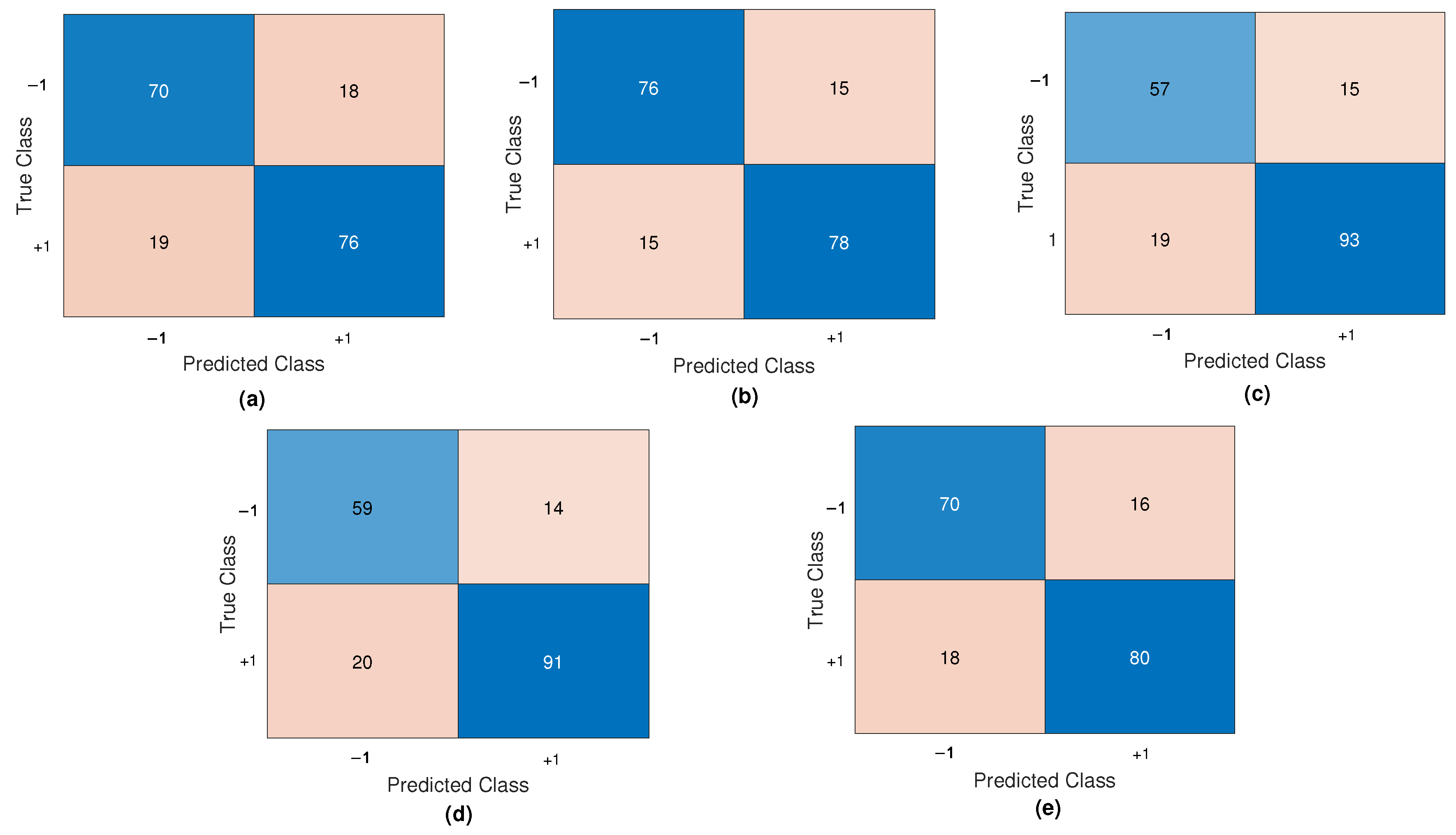
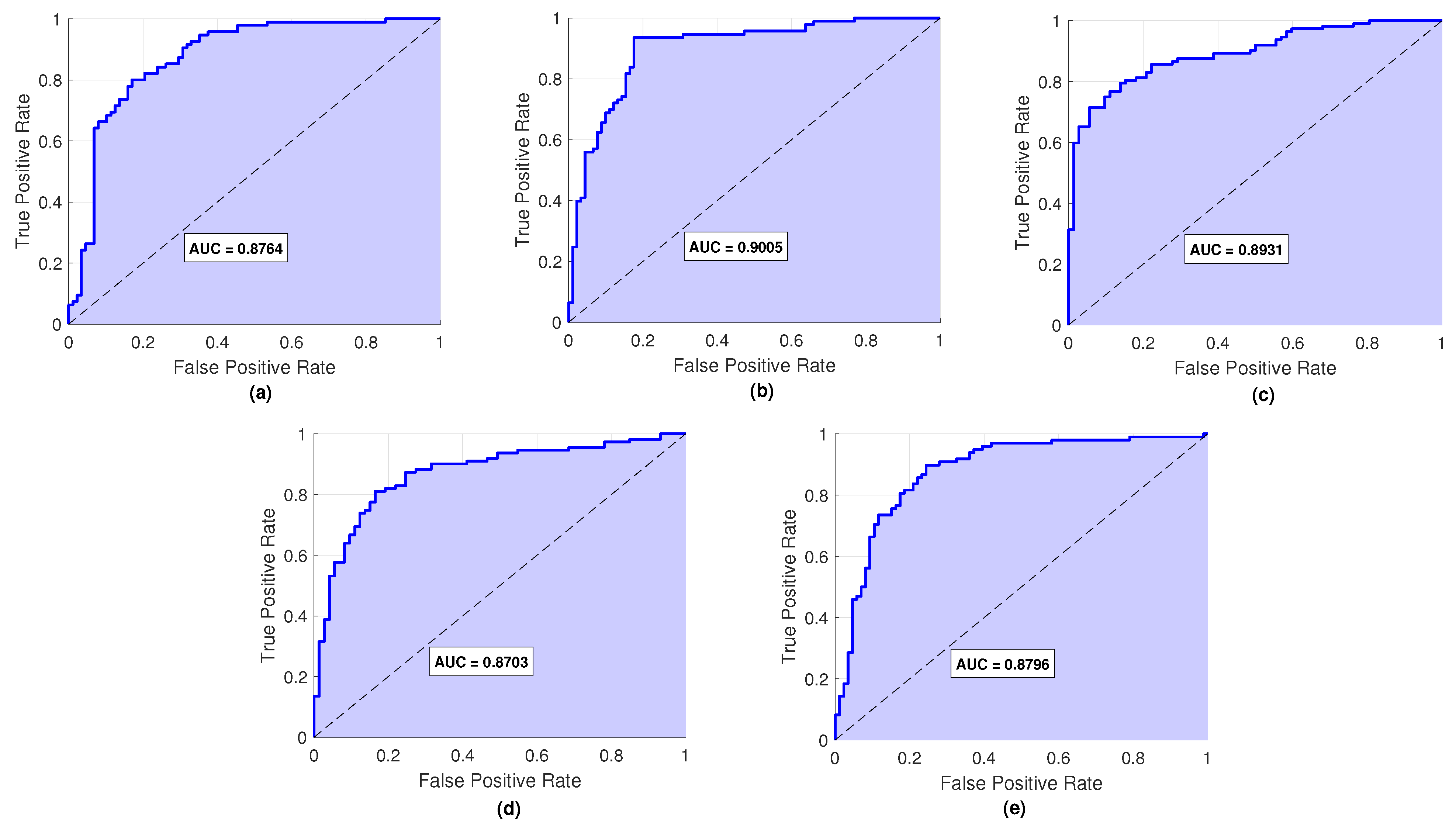
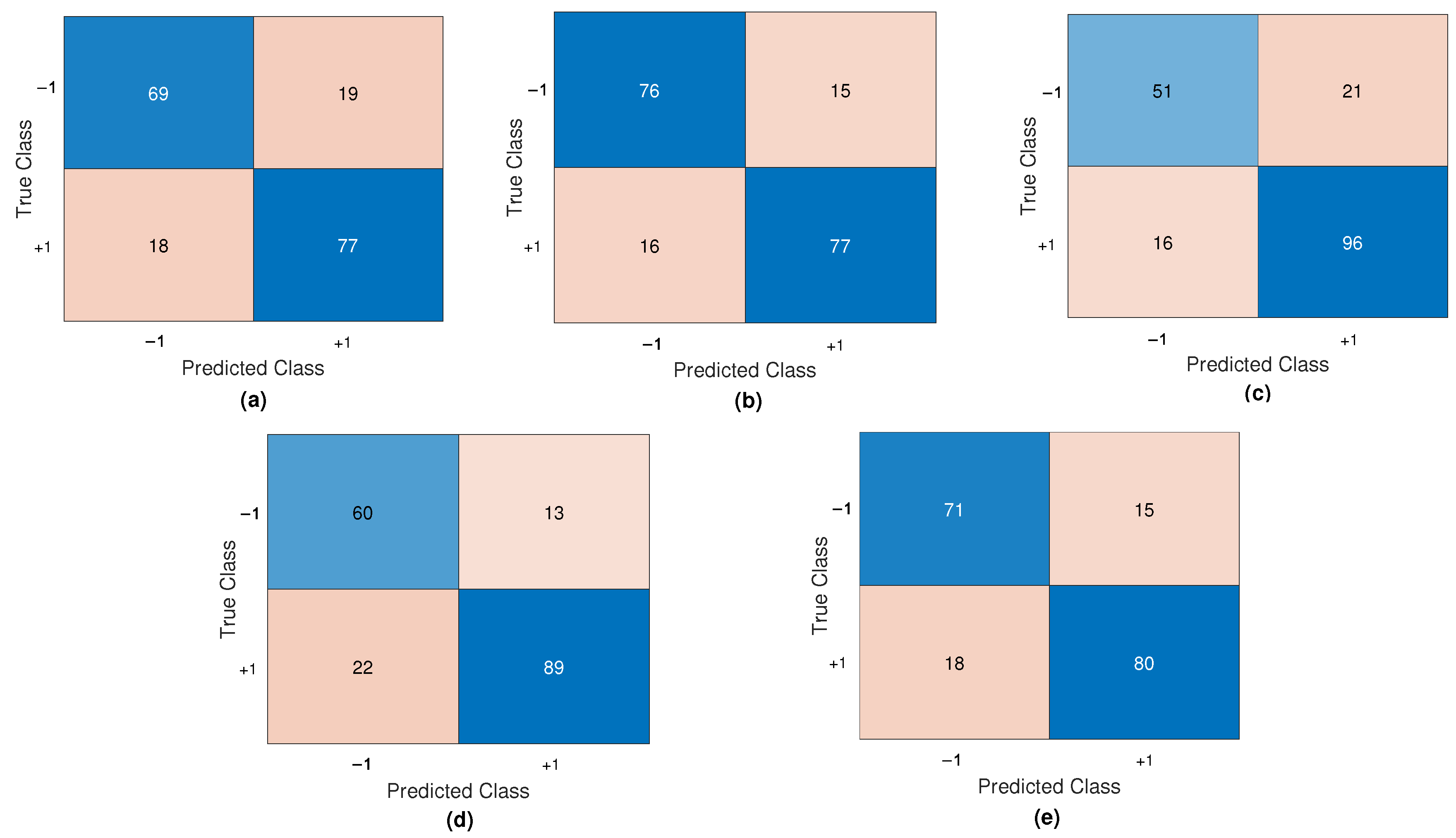
These results show that the training performance is consistent across all five folds. Specifically, the number of SVs and the margin have similar characteristics, which is evident from the mean values calculated for each metric during training. Validation indicates strong generalization performance for the SVM-MSMOH model, particularly with the model from fold 2. This is evident from the balanced metrics: accuracy of $83.6956\%$, sensitivity of $83.8710\%$, specificity of $83.5165\%$, precision of $83.8710\%$, and an F1-score of $0.8387$ as seen in Table 10. This is corroborated from the standard deviation obtained and the confusion matrices for each fold in Figure 9 where (−1) indicates the heart disease presence while (+1) indicates no heart disease presence. Furthermore the ROC curve is illustrated in Figure 10. As previously noted, the second model, illustrated in Figure 10b, yields an AUC of 0.9005, confirming it as the best-performing model.

In contrast, results obtained with the conventional SVM-SMOH are presented in

Table 11. Heart disease classification training metrics with SVM-SMOH in cross-validation with 5 folds.

Fold	Accuracy in Training	Sensitivity in Training	Specificity in Training	Precision in Training	F1-Score in Training	SVs	Margin
1	$82.2010\%$	$83.5749\%$	$80.4348\%$	$84.5966\%$	$0.8408$	319	1.7052
2	$81.9047\%$	$82.9327\%$	$80.5643\%$	$84.7666\%$	$0.8383$	377	1.8417
3	$81.9047\%$	$83.1234\%$	$80.4734\%$	$83.3333\%$	$0.8322$	431	1.7455
4	$81.7687\%$	$81.6583\%$	$81.8991\%$	$84.1969\%$	$0.8290$	316	1.6508
5	$82.0408\%$	$82.9684\%$	$80.8642\%$	$84.6154\%$	$0.8378$	323	1.8170
Mean	81.9639%	84.8515%	80.8471%	84.3017%	0.8356	353.2	1.7520
Standard Deviation	0.1637%	0.7144%	0.6117%	0.5810%	0.0049	50.2116	0.0787

where the same fold partition as selected in the previous MSMOH is used for the classification task. Performance indicates significant differences with the proposed modification specifically in the number of SVs needed to construct the optimal hyperplane and a margin maximization which is smaller than the one obtained in the MSMOH with less SVs.

Despite similarity in training metrics, average performance shows that MSMOH achieved better accuracy ($81.9911\%$) compared to SMOH ($81.9639\%$). Although SMOH offers better average metrics during training, its testing performance is not entirely consistent.

In contrast, MSMOH provides similar and, in some metrics, superior results compared to SMOH, while using fewer SVs and a wider margin. This is reflected in the model’s better generalization ability, as shown in

Table 12. Heart disease classification test metrics with SVM-SMOH in cross-validation with 5 folds.

Fold	Accuracy in Test	Sensitivity in Test	Specificity in Test	Precision in Test	F1-Score in Test
1	$79.7814\%$	$81.0526\%$	$78.4091\%$	$80.2083\%$	$0.8062$
2	$83.1521\%$	$82.7957\%$	$83.5165\%$	$83.6957\%$	$0.8324$
3	$79.8913\%$	$85.7143\%$	$70.8333\%$	$82.0513\%$	$0.8384$
4	$80.9782\%$	$80.1802\%$	$82.1918\%$	$87.2549\%$	$0.8356$
5	$82.0652\%$	$81.6327\%$	$82.5581\%$	$84.2105\%$	$0.8290$
Mean	81.1736%	82.2750%	79.5017%	83.4841%	0.8283
Standard Deviation	1.4431%	2.1445%	5.2209%	2.6256%	0.0129

, where the average results for each metric indicate that MSMOH outperforms SMOH in many categories.

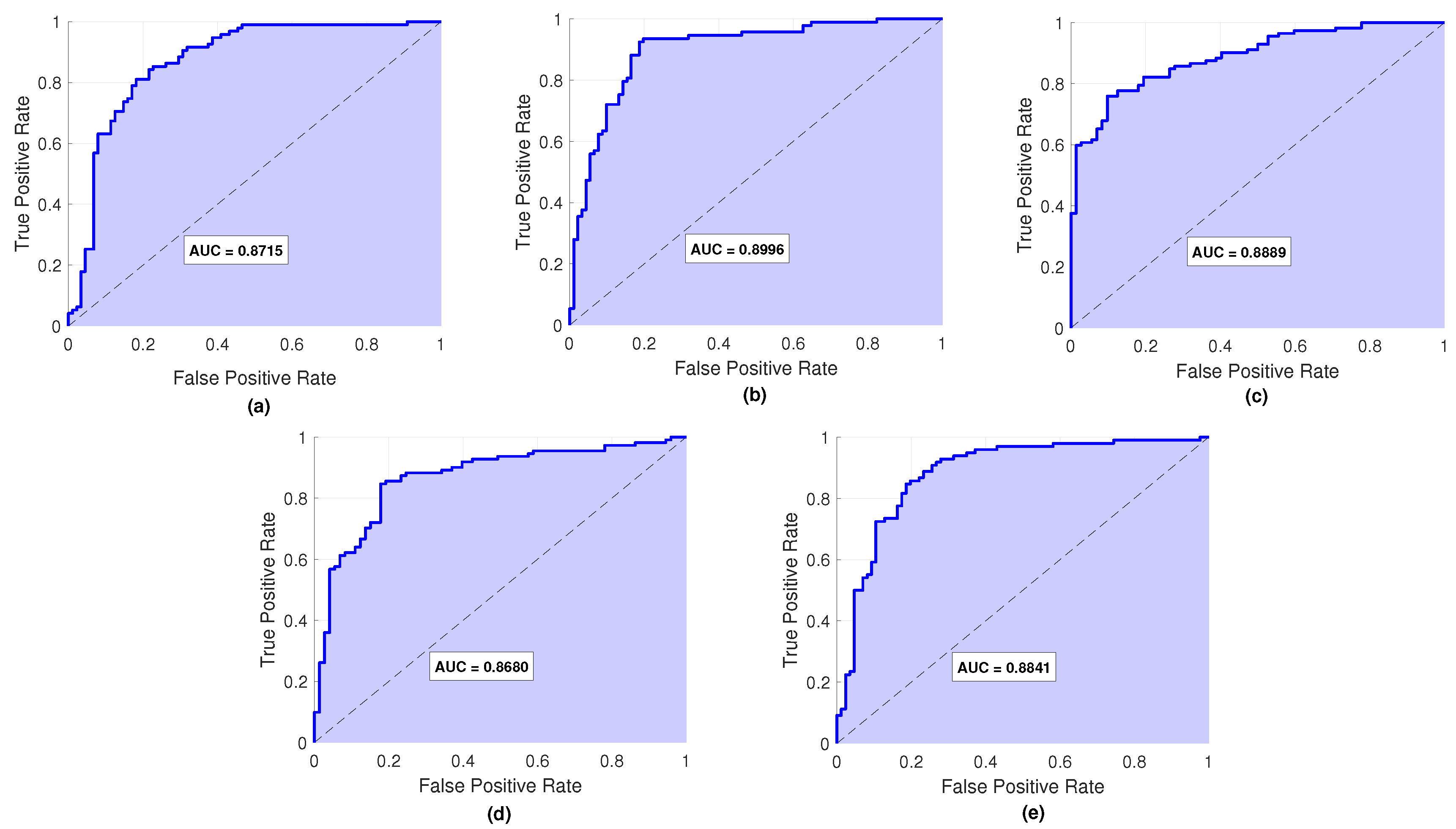
In addition, the standard deviation is higher in metrics such as sensitivity, specificity, and precision. Furthermore, the confusion matrices in Figure 11 and the ROC curves in Figure 12 highlight the classification performance and the model’s generalization ability. For comparison, the best SMOH is also obtained from fold 2, but it had a smaller AUC value of 0.8996, as shown in Figure 12b.

This analysis revealed that SVM-MSMOH consistently achieved balanced and high-quality performance metrics, with model form fold 2 being particularly effective (AUC = 0.9005). In a direct comparison with the SVM-SMOH model, SVM-MSMOH demonstrated crucial advantages: it required fewer SVs, created a wider margin, and showed superior generalization performance on unseen data, even with similar training metrics.

These results, supported with detailed metrics and visualizations, indicate the effectiveness of proposed modification for building a more robust and efficient model. To assure a better comparison between SVM-MSMOH and SVM-SMOH, the Mean Absolute Generalization Gap (MAGG) is computed using Equation (51) to assess the stability and generalization performance. MAGG is defined as the average of the absolute differences between training and test performance for each metric, and the results are presented in

Table 13. SVM-MSMOH and SVM-SMOH (5-fold cross-validation) GAPP comparison.

Metric	Training (MSMOH)	Test (MSMOH)	Training (SMOH)	Test (SMOH)
Accuracy (%)	81.9911	81.6084	81.9639	81.1736
Sensitivity (%)	82.9949	82.1042	84.8515	82.2750
Specificity (%)	80.7062	80.8891	80.8471	79.5017
Precision (%)	84.2516	84.1666	84.3017	83.4841
F1-Score	0.8361	0.8311	0.8356	0.8409
MAGG	0.3092		1.1070

:

$$MAGG={\displaystyle \frac{1}{mt}}{\displaystyle \sum _{m=1}^{mt}}\left|metri{c}_{training}^{\left(m\right)}-metri{c}_{test}^{\left(m\right)}\right|$$

(51)

where $metri{c}_{training}$ is the value obtained in the m training metric, $metri{c}_{test}$ is the value obtained in the m test metric, and $m=1,2,\dots ,mt$ is the metric measured for each model.

The SVM-MSMOH model has a smaller difference between training and test performance resulting in a MAGG of $0.3092$. On the other hand, the SVM-SMOH model has a MAGG of $1.1070$. The standard deviation obtained for each metric also helps to analyze the generalization capacity of MSMOH and SMOH. In the case of MSMOH, the standard deviation in the training and test sets is ≤2.5; while in the training of SMOH, the standard deviation accomplishes this condition, in the test, the standard deviation is ≥2.5. This indicate that SVM-MSMOH has a better generalization capacity.

6. Neural Associative Memory with MSMOH Training for Fault Diagnosis in Fossil Electric Power Plants

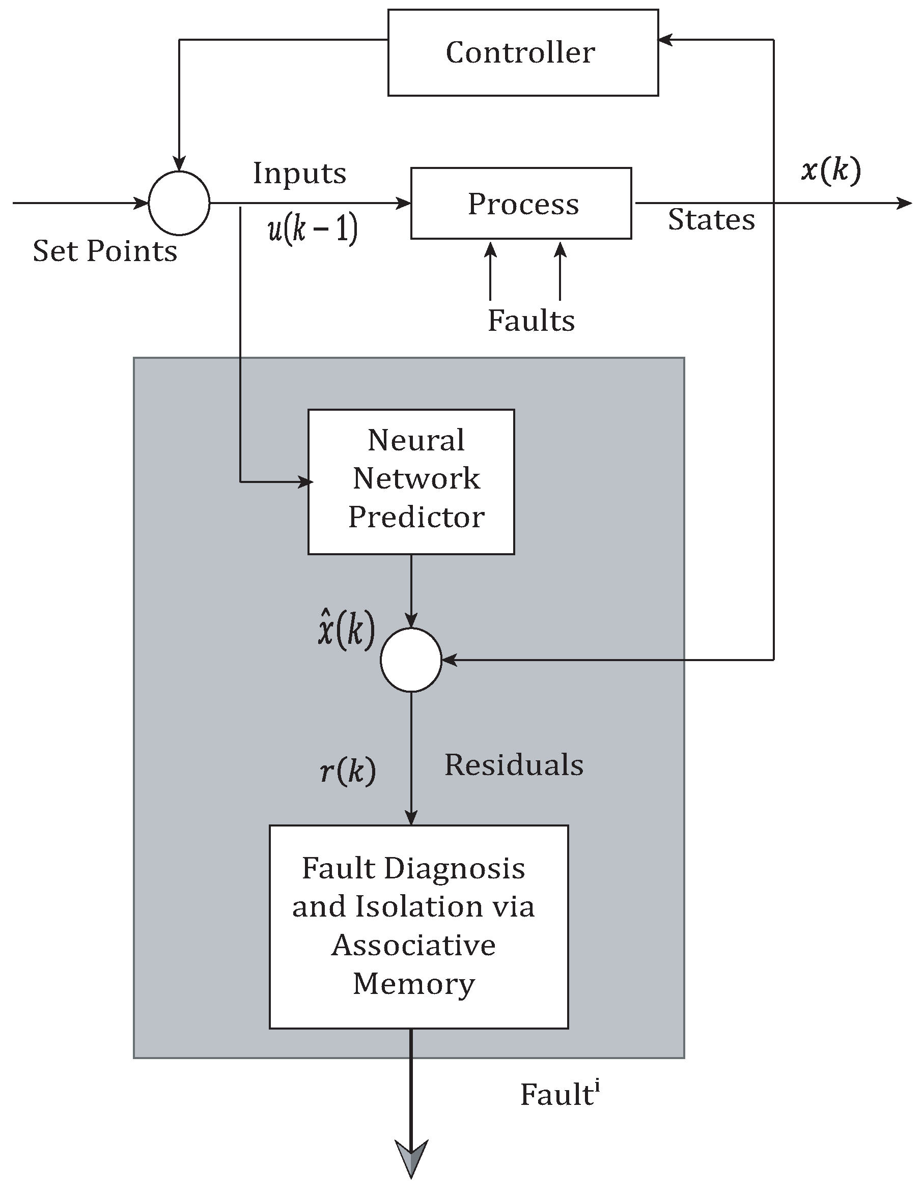
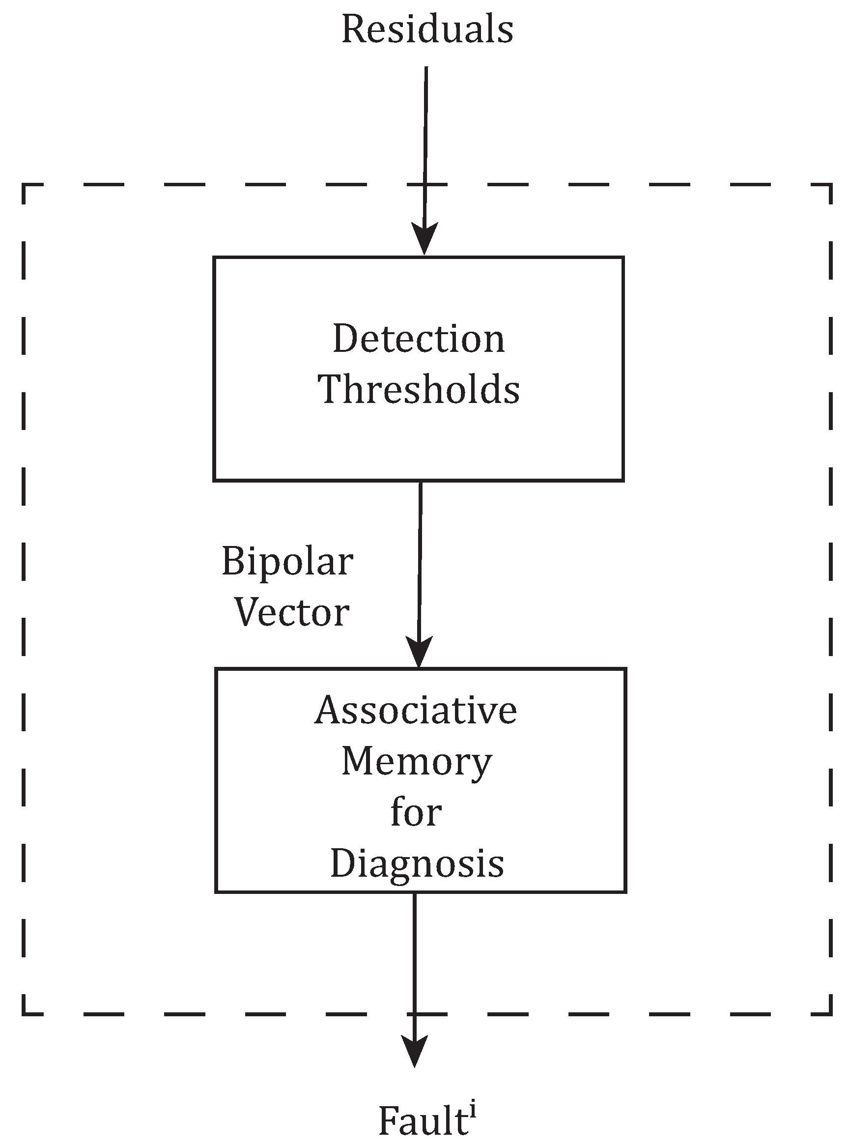
In this section, the previously presented MSMOH is employed to find optimal values of a NAM used for fault diagnosis. The scheme for fault diagnosis is presented where the scheme has two components: residual generation and fault diagnosis [17]. The scheme is displayed in Figure 13. The first component relies on a comparison between measurements obtained from the plant and corresponding predicted values generated by a neural network predictor. This predictor is developed using neural network models trained with healthy operational data from the plant. Discrepancies between these two sets of values, termed residuals, provide a robust indicator for detecting faults. The calculation of these residuals is as follows:

$$\begin{array}{ccc}\hfill r_i\left(k\right)& =& x_i\left(k\right)-\widehat{x_i}\left(k\right).i=1,2,\dots ,n\hfill \end{array}$$

(52)

Variables $x_i\left(k\right)$ denote the actual plant measurements, while $\widehat{x_i}\left(k\right)$ are the corresponding predicted values. Ideally, under normal plant operation, these residuals should remain consistent regardless of system’s operating state, indicating only the presence of noise and minor disturbance. A fault in the system, however, will cause the residuals to deviate from zero in identifiable ways. For the second component, residuals are converted into bipolar or binary fault patterns through the application of thresholds. These patterns are crucial for training a NAM based on a recurrent neural network designed to perform fault diagnosis. Associative memory itself is trained using the MSMOH algorithm. After the previous stage, residual vectors are generated with ten elements which are evaluated by detection thresholds.

Detection thresholds are contained in

Table 14. Detection thresholds.

i	${\mathit{\tau }}_{\mathit{i}}$	Variables
1	$\pm 25$ MW	Load power
2	$\pm 30$ Pa	Boiler pressure
3	$\pm 0.022$ m	Drum level
4	$\pm 4 °\mathrm{K}$	Reheated steam temperature
5	$\pm 10 °\mathrm{K}$	Superheated steam pressure
6	±20,000 Pa	Reheated steam pressure
7	±42,000 Pa	Drum pressure
8	$\pm 0.85\%$	Differential pressure (spray steam-fossil oil flow)
9	$\pm 0.24 °\mathrm{K}$	Fossil oil temperature to burners
10	$\pm 10 °\mathrm{K}$	Feed-water Temperature

.

This evaluation provides a set of residuals encoded as bipolar vectors $[s_1\left(k\right),s_2\left(k\right),\dots ,s_{10}\left(k\right)]$ obtained with Equation (53):

$$\begin{array}{c}\hfill s\left(i\right)=\left\{\begin{array}{cc}-1,\hfill & r_i<{\tau }_i\hfill \\ 1,\hfill & r_i\ge {\tau }_i\hfill \end{array}\right.\end{array}i=1,2,\dots ,10$$

(53)

Residuals are encoded in real-time for every detected fault. Subsequently, these encoded patterns undergo analysis to identify and select the most appropriate fault patterns for storage in associative memory. This crucial selection step ensures accurate fault discrimination, reduces incidence of false alarms, and facilitates prompt fault isolation. The procedure is illustrated in Figure 14.

Fault patterns are described in

Table 15. Fault patterns.

${\mathit{F}}_0$	${\mathit{F}}_1$	${\mathit{F}}_2$	${\mathit{F}}_3$	${\mathit{F}}_4$	${\mathit{F}}_5$	${\mathit{F}}_6$
−1	1	−1	−1	−1	−1	1
−1	1	−1	−1	−1	−1	−1
−1	1	1	1	1	1	1
−1	1	−1	1	−1	−1	−1
−1	1	1	1	−1	−1	1
−1	1	−1	1	−1	1	1
−1	1	1	1	1	−1	1
−1	−1	−1	−1	−1	−1	1
−1	1	−1	−1	−1	1	1
−1	1	−1	−1	−1	−1	1

where each column corresponds, respectively, to the following:

• $F_0$: Normal Operating Conditions;
• $F_1$: Water Wall Tube Rupture;
• $F_2$: Superheater Tube Rupture;
• $F_3$: Superheated Steam Temperature Control Failure;
• $F_4$: Fouled Regenerative Preheater;
• $F_5$: Feedwater Pump Variable Speed Drive Operating at Maximum;
• $F_6$: Stuck Fuel Valve.

6.1. Results on Fault Diagnosis

This section details the training of the NAM (as described in Section 3) using four algorithms: training, OH, SMOH, and proposed MSMOH. The resulting $\mathrm{\Lambda }$, T, W, I, and B matrices are presented and used in the NAM defined in Equation (22) along with convergence of stored patterns specifically achieved with MSMOH training. A convergence analysis is also conducted to demonstrate the number of elements that converge to the seven stored fault patterns. From a total of 1024 $\left(2^{10}\right)$ possible combinations, the number of convergent, non-convergent, and spurious memories for each model are shown, demonstrating how many elements converge to 7 store fault patterns.

6.1.1. Results with Perceptron Training Algorithm

For the perceptron training algorithm, the parameters considered are as follows: $\mu =7$, $\eta =0.1$, and $A=1$ which have been taken from [23].

$$W_P=\left[\begin{array}{cccccccccc}-15.2000& 3.7000& -0.7000& 0.9000& 2.9000& 2.3000& 1.5000& 4.1000& 5.1000& 7.3000\\ 4.4000& -10.9000& -3.4000& 8.2000& -0.2000& -0.6000& -1.6000& -3.2000& 2.6000& 4.4000\\ -0.5000& -2.9000& -8.8000& -1.3000& 3.1000& 5.3000& 9.3000& -3.5000& 3.7000& -0.5000\\ -0.1000& 6.1000& -1.5000& -6.6000& 3.1000& 7.1000& 1.3000& -4.3000& -2.9000& -0.1000\\ 11.7000& -2.9000& 9.3000& 18.3000& 0.4000& 10.9000& 31.3000& 7.1000& -10.3000& 11.7000\\ 1.1000& -1.9000& 4.5000& 7.1000& 1.7000& -6.6000& -1.5000& -1.1000& 7.1000& 1.1000\\ 1.9000& -0.9000& 7.9000& 1.3000& 6.7000& -2.9000& -7.5000& -0.9000& -5.1000& 1.9000\\ 4.3000& -3.5000& -2.9000& -4.9000& 1.5000& 0.1000& -0.1000& -8.1000& 1.5000& 4.3000\\ 4.6000& 1.6000& 3.6000& -3.8000& -2.6000& 7.0000& -4.2000& 0.4000& -10.1000& 4.6000\\ 7.3000& 3.7000& -0.7000& 0.9000& 2.9000& 2.3000& 1.5000& 4.1000& 5.1000& -15.2000\end{array}\right]$$

(54)

$$T_P=\left[\begin{array}{cccccccccc}-8.200& 3.7000& -0.7000& 0.9000& 2.9000& 2.3000& 1.5000& 4.1000& 5.1000& 7.3000\\ 4.4000& -3.9000& -3.4000& 8.2000& -0.2000& -0.6000& -1.6000& -3.2000& 2.6000& 4.4000\\ -0.5000& -2.9000& -1.800& -1.3000& 3.1000& 5.3000& 9.3000& -3.5000& 3.7000& -0.5000\\ -0.1000& 6.1000& -1.5000& 0.4000& 3.1000& 7.1000& 1.3000& -4.3000& -2.9000& -0.1000\\ 11.7000& -2.9000& 9.3000& 18.3000& 7.4000& 10.9000& 31.3000& 7.1000& -10.3000& 11.7000\\ 1.1000& -1.9000& 4.5000& 7.1000& 1.7000& 0.4000& -1.5000& -1.1000& 7.1000& 1.1000\\ 1.9000& -0.9000& 7.9000& 1.3000& 6.7000& -2.9000& -0.5000& -0.9000& -5.1000& 1.9000\\ 4.3000& -3.5000& -2.9000& -4.9000& 1.5000& 0.1000& -0.1000& -1.1000& 1.5000& 4.3000\\ 4.6000& 1.6000& 3.6000& -3.8000& -2.6000& 7.0000& -4.2000& 0.4000& -3.1000& 4.6000\\ 7.3000& 3.7000& -0.7000& 0.9000& 2.9000& 2.3000& 1.5000& 4.1000& 5.1000& -8.2000\end{array}\right]$$

(55)

$$I_P={\left[\begin{array}{cccccccccc}-2.5000& -5.8000& 3.9000& -3.9000& 5.5000& 2.1000& 1.7000& -8.5000& 0.6000& -2.5000\end{array}\right]}^T$$

(56)

6.1.2. Results with OH Training Algorithm

For consistency, parameters for OH, SMOH, and MSMOH training $\mu =1.6486$, $C=0.6322$, and $A=1.22$ are selected through trial and error. The steps followed to acquire these matrices are described in Section 3.1.

$${\mathrm{\Lambda }}_{OH}=\left[\begin{array}{cccccccccc}0.0000& 0.0000& 0.3000& 0.0000& 0.0000& 0.0556& 0.1796& 0.0000& 0.0971& 0.0000\\ 0.0833& 0.2273& 0.0000& 0.0833& 0.0000& 0.0000& 0.0097& 0.1364& 0.0728& 0.0833\\ 0.0093& 0.0000& 0.0000& 0.1759& 0.5000& 0.2037& 0.0000& 0.0455& 0.0000& 0.0093\\ 0.0926& 0.0909& 0.0000& 0.2407& 0.0000& 0.1852& 0.0146& 0.0000& 0.1408& 0.0926\\ 0.0000& 0.0000& 0.2000& 0.0000& 0.5000& 0.0556& 0.2621& 0.0000& 0.0340& 0.0000\\ 0.0556& 0.0000& 0.1000& 0.0556& 0.0000& 0.1111& 0.1408& 0.0455& 0.1942& 0.0556\\ 0.0741& 0.1364& 0.0000& 0.0926& 0.0000& 0.0185& 0.0340& 0.2273& 0.0049& 0.0741\end{array}\right]$$

(57)

$$b_{OH}={\left[\begin{array}{cccccccccc}-0.0741& -0.5000& 0.4000& -0.3704& 0.0000& 0.3704& 0.0347& -0.7273& 0.0097& -0.0741\end{array}\right]}^T$$

(58)

$$W_{OH}=\left[\begin{array}{cccccccccc}0.3148& 0.1667& 0.0000& -0.0185& 0.1111& 0.0185& 0.1111& 0.1481& 0.2037& 0.3148\\ 0.1818& 0.4545& 0.0000& 0.2727& 0.0000& 0.0000& 0.0000& -0.2727& 0.1818& 0.1818\\ 0.0000& 0.0000& 0.6000& 0.0000& 0.0001& 0.2000& 0.4000& 0.0000& 0.2000& 0.0000\\ -0.0185& 0.1667& 0.0000& 0.6481& 0.1111& 0.3519& 0.1111& -0.1852& -0.1296& -0.0185\\ 0.0000& 0.0000& 0.0000& 0.0000& 1.0000& 0.0000& 0.0001& 0.0000& 0.0000& 0.0000\\ 0.0370& 0.0000& 0.1111& 0.3704& 0.0000& 0.6296& -0.1111& 0.0370& 0.2593& 0.0370\\ 0.0874& 0.0194& 0.3592& 0.0485& 0.1165& -0.1650& 0.6408& 0.0680& -0.1942& 0.0874\\ 0.1818& -0.2727& 0.0000& -0.2727& 0.0909& 0.0909& 0.0909& 0.4545& 0.0909& 0.1818\\ 0.1553& 0.1456& 0.1942& -0.1359& -0.1262& 0.2621& -0.1942& 0.0097& 0.5437& 0.1553\\ 0.3148& 0.1667& 0.0000& -0.0185& 0.1111& 0.0185& 0.1111& 0.1481& 0.2037& 0.3148\end{array}\right]$$

(59)

$$T_{OH}=\left[\begin{array}{cccccccccc}0.9634& 0.1667& 0.0000& -0.0185& 0.1111& 0.0185& 0.1111& 0.1481& 0.2037& 0.3148\\ 0.1818& 1.1031& 0.0000& 0.2727& 0.0000& 0.0000& 0.0000& -0.2727& 0.1818& 0.1818\\ 0.0000& 0.0000& 1.2486& 0.0000& 0.0001& 0.2000& 0.4000& 0.0000& 0.2000& 0.0000\\ -0.0185& 0.1667& 0.0000& 1.2967& 0.1111& 0.3519& 0.1111& -0.1852& -0.1296& -0.0185\\ 0.0000& 0.0000& 0.0000& 0.0000& 1.6486& 0.0000& 0.0001& 0.0000& 0.0000& 0.0000\\ 0.0370& 0.0000& 0.1111& 0.3704& 0.0000& 1.2782& -0.1111& 0.0370& 0.2593& 0.0370\\ 0.0874& 0.0194& 0.3592& 0.0485& 0.1165& -0.1650& 1.2894& 0.0680& -0.1942& 0.0874\\ 0.1818& -0.2727& 0.0000& -0.2727& 0.0909& 0.0909& 0.0909& 1.1031& 0.0909& 0.1818\\ 0.1553& 0.1456& 0.1942& -0.1359& -0.1262& 0.2621& -0.1942& 0.0097& 1.1923& 0.1553\\ 0.3148& 0.1667& 0.0000& -0.0185& 0.1111& 0.0185& 0.1111& 0.1481& 0.2037& 0.9634\end{array}\right]$$

(60)

$$I_{OH}={\left[\begin{array}{cccccccccc}-0.0741& -0.5000& 0.4000& -0.3704& 0.0000& 0.3704& 0.0347& -0.7273& 0.0097& -0.0741\end{array}\right]}^T$$

(61)

6.1.3. Results with SMOH Training Algorithm

Results obtained with the SMOH training using steps described in Section 3.2 with the same parameters previously described.

$${\mathrm{\Lambda }}_{SMOH}=\left[\begin{array}{cccccccccc}0.0000& 0.0000& 0.3000& 0.0000& 0.0000& 0.0556& 0.1796& 0.0000& 0.0971& 0.0000\\ 0.0833& 0.2273& 0.0000& 0.0833& 0.0000& 0.0000& 0.0097& 0.1364& 0.0728& 0.0833\\ 0.0093& 0.0000& 0.0000& 0.1759& 0.5000& 0.2037& 0.0000& 0.0455& 0.0000& 0.0093\\ 0.0926& 0.0909& 0.0000& 0.2407& 0.0000& 0.1852& 0.0146& 0.0000& 0.1408& 0.0926\\ 0.0000& 0.0000& 0.2000& 0.0000& 0.5000& 0.0556& 0.2621& 0.0000& 0.0340& 0.0000\\ 0.0556& 0.0000& 0.1000& 0.0556& 0.0000& 0.1111& 0.1408& 0.0455& 0.1942& 0.0556\\ 0.0741& 0.1364& 0.0000& 0.0926& 0.0000& 0.0185& 0.0340& 0.2273& 0.0049& 0.0741\end{array}\right]$$

(62)

$$b_{SMOH}={\left[\begin{array}{cccccccccc}-0.0370& -0.5455& 0.4000& -0.3704& 0.0000& 0.3704& 0.0680& -0.7273& 0.0097& -0.0370\end{array}\right]}^T$$

(63)

$$W_{SMOH}=\left[\begin{array}{cccccccccc}0.3148& 0.1667& 0.0000& -0.0185& 0.1111& 0.0185& 0.1111& 0.1481& 0.2037& 0.3148\\ 0.1818& 0.4545& 0.0000& 0.2727& 0.0000& 0.0000& 0.0000& -0.2727& 0.1818& 0.1818\\ 0.0000& 0.0000& 0.6000& 0.0000& 0.0000& 0.2000& 0.4000& 0.0000& 0.2000& 0.0000\\ -0.0185& 0.1667& 0.0000& 0.6481& 0.1111& 0.3519& 0.1111& -0.1852& -0.1296& -0.0185\\ 0.0000& 0.0000& 0.0000& 0.0000& 1.0000& 0.0000& 0.0001& 0.0000& 0.0000& 0.0000\\ 0.0370& 0.0000& 0.1111& 0.3704& 0.0000& 0.6296& -0.1111& 0.0370& 0.2593& 0.0370\\ 0.0874& 0.0194& 0.3592& 0.0485& 0.1165& -0.1650& 0.6408& 0.0680& -0.1942& 0.0874\\ 0.1818& -0.2727& 0.0000& -0.2727& 0.0909& 0.0909& 0.0909& 0.4545& 0.0909& 0.1818\\ 0.1553& 0.1456& 0.1942& -0.1359& -0.1262& 0.2621& -0.1942& 0.0097& 0.5437& 0.1553\\ 0.3148& 0.1667& 0.0000& -0.0185& 0.1111& 0.0185& 0.1111& 0.1481& 0.2037& 0.3148\end{array}\right]$$

(64)

$$T_{SMOH}=\left[\begin{array}{cccccccccc}0.9634& 0.1667& 0.0000& -0.0185& 0.1111& 0.0185& 0.1111& 0.1481& 0.2037& 0.3148\\ 0.1818& 1.1031& 0.0000& 0.2727& 0.0000& 0.0000& 0.0000& -0.2727& 0.1818& 0.1818\\ 0.0000& 0.0000& 1.2486& 0.0000& 0.0000& 0.2000& 0.4000& 0.0000& 0.2000& 0.0000\\ -0.0185& 0.1667& 0.0000& 1.2967& 0.1111& 0.3519& 0.1111& -0.1852& -0.1296& -0.0185\\ 0.0000& 0.0000& 0.0000& 0.0000& 1.6486& 0.0000& 0.0001& 0.0000& 0.0000& 0.0000\\ 0.0370& 0.0000& 0.1111& 0.3704& 0.0000& 1.2782& -0.1111& 0.0370& 0.2593& 0.0370\\ 0.0874& 0.0194& 0.3592& 0.0485& 0.1165& -0.1650& 1.2894& 0.0680& -0.1942& 0.0874\\ 0.1818& -0.2727& 0.0000& -0.2727& 0.0909& 0.0909& 0.0909& 1.1031& 0.0909& 0.1818\\ 0.1553& 0.1456& 0.1942& -0.1359& -0.1262& 0.2621& -0.1942& 0.0097& 1.1923& 0.1553\\ 0.3148& 0.1667& 0.0000& -0.0185& 0.1111& 0.0185& 0.1111& 0.1481& 0.2037& 0.9634\end{array}\right]$$

(65)

$$I_{SMOH}={\left[\begin{array}{cccccccccc}-0.0370& -0.5455& 0.4000& -0.3704& 0.0000& 0.3704& 0.0680& -0.7273& 0.0097& -0.0370\end{array}\right]}^T$$

(66)

6.1.4. Results with MSMOH Training Algorithm

For the NAM training in this section, the same parameters as the OH and SMOH algorithms are used. Additionally, with $p=2$, Equation (47) was used to obtain the NAM training matrices.

$${\mathrm{\Lambda }}_{MSMOH}=\left[\begin{array}{cccccccccc}0.0000& 0.0000& 0.2550& 0.0000& 0.0101& 0.0562& 0.1487& 0.0000& 0.0810& 0.0000\\ 0.0759& 0.2000& 0.0000& 0.0868& 0.0000& 0.0000& 0.0075& 0.1178& 0.0634& 0.0759\\ 0.0163& 0.0000& 0.0236& 0.1442& 0.3154& 0.1564& 0.0000& 0.0418& 0.0000& 0.0163\\ 0.0797& 0.0815& 0.0000& 0.2008& 0.0379& 0.1553& 0.0253& 0.0000& 0.1234& 0.0797\\ 0.0000& 0.0000& 0.1428& 0.0000& 0.3223& 0.0704& 0.2122& 0.0000& 0.0419& 0.0000\\ 0.0526& 0.0000& 0.0886& 0.0528& 0.0416& 0.1097& 0.1311& 0.0418& 0.1698& 0.0526\\ 0.0727& 0.1185& 0.0000& 0.0906& 0.0207& 0.0182& 0.0349& 0.2013& 0.0132& 0.0727\end{array}\right]$$

(67)

$$b_{MSMOH}={\left[\begin{array}{cccccccccc}-0.0020& -0.5000& 0.4457& -0.3535& 0.0641& 0.3256& 0.1109& -0.7013& 0.0335& -0.0020\end{array}\right]}^T$$

(68)

$$W_{MSMOH}=\left[\begin{array}{cccccccccc}0.2973& 0.1518& 0.0000& -0.0076& 0.1052& 0.0327& 0.1052& 0.1455& 0.1921& 0.2973\\ 0.1629& 0.4000& 0.0000& 0.2370& 0.0000& 0.0000& 0.0000& -0.2370& 0.1629& 0.1629\\ 0.0000& 0.0000& 0.5099& 0.0000& 0.0472& 0.1771& 0.3328& 0.0000& 0.1771& 0.0000\\ -0.0076& 0.1735& 0.0000& 0.5752& 0.1056& 0.2884& 0.1056& -0.1811& -0.1132& -0.0076\\ 0.0414& 0.0000& 0.0202& 0.0757& 0.7479& 0.0340& 0.1033& 0.0414& -0.0417& 0.0414\\ 0.0363& 0.0000& 0.1125& 0.3105& 0.0340& 0.5662& -0.1069& 0.0363& 0.2557& 0.0363\\ 0.0848& 0.0150& 0.2975& 0.0656& 0.1353& -0.1270& 0.5598& 0.0698& -0.1775& 0.0848\\ 0.1671& -0.2356& 0.0000& -0.2356& 0.0835& 0.0835& 0.0835& 0.4027& 0.0835& 0.1671\\ 0.1533& 0.1268& 0.1621& -0.1201& -0.0936& 0.2459& -0.1775& 0.0265& 0.4928& 0.1533\\ 0.2973& 0.1518& 0.0000& -0.0076& 0.1052& 0.0327& 0.1052& 0.1455& 0.1921& 0.2973\end{array}\right]$$

(69)

$$T_{MSMOH}=\left[\begin{array}{cccccccccc}0.9459& 0.1518& 0.0000& -0.0076& 0.1052& 0.0327& 0.1052& 0.1455& 0.1921& 0.2973\\ 0.1629& 1.0486& 0.0000& 0.2370& 0.0000& 0.0000& 0.0000& -0.2370& 0.1629& 0.1629\\ 0.0000& 0.0000& 1.1585& 0.0000& 0.0472& 0.1771& 0.3328& 0.0000& 0.1771& 0.0000\\ -0.0076& 0.1735& 0.0000& 1.2238& 0.1056& 0.2884& 0.1056& -0.1811& -0.1132& -0.0076\\ 0.0414& 0.0000& 0.0202& 0.0757& 1.3965& 0.0340& 0.1033& 0.0414& -0.0417& 0.0414\\ 0.0363& 0.0000& 0.1125& 0.3105& 0.0340& 1.2148& -0.1069& 0.0363& 0.2557& 0.0363\\ 0.0848& 0.0150& 0.2975& 0.0656& 0.1353& -0.1270& 1.2084& 0.0698& -0.1775& 0.0848\\ 0.1671& -0.2356& 0.0000& -0.2356& 0.0835& 0.0835& 0.0835& 1.0513& 0.0835& 0.1671\\ 0.1533& 0.1268& 0.1621& -0.1201& -0.0936& 0.2459& -0.1775& 0.0265& 1.1414& 0.1533\\ 0.2973& 0.1518& 0.0000& -0.0076& 0.1052& 0.0327& 0.1052& 0.1455& 0.1921& 0.9459\end{array}\right]$$

(70)

$$I_{MSMOH}={\left[\begin{array}{cccccccccc}-0.0020& -0.5000& 0.4457& -0.3535& 0.0641& 0.3256& 0.1109& -0.7013& 0.0335& -0.0020\end{array}\right]}^T$$

(71)

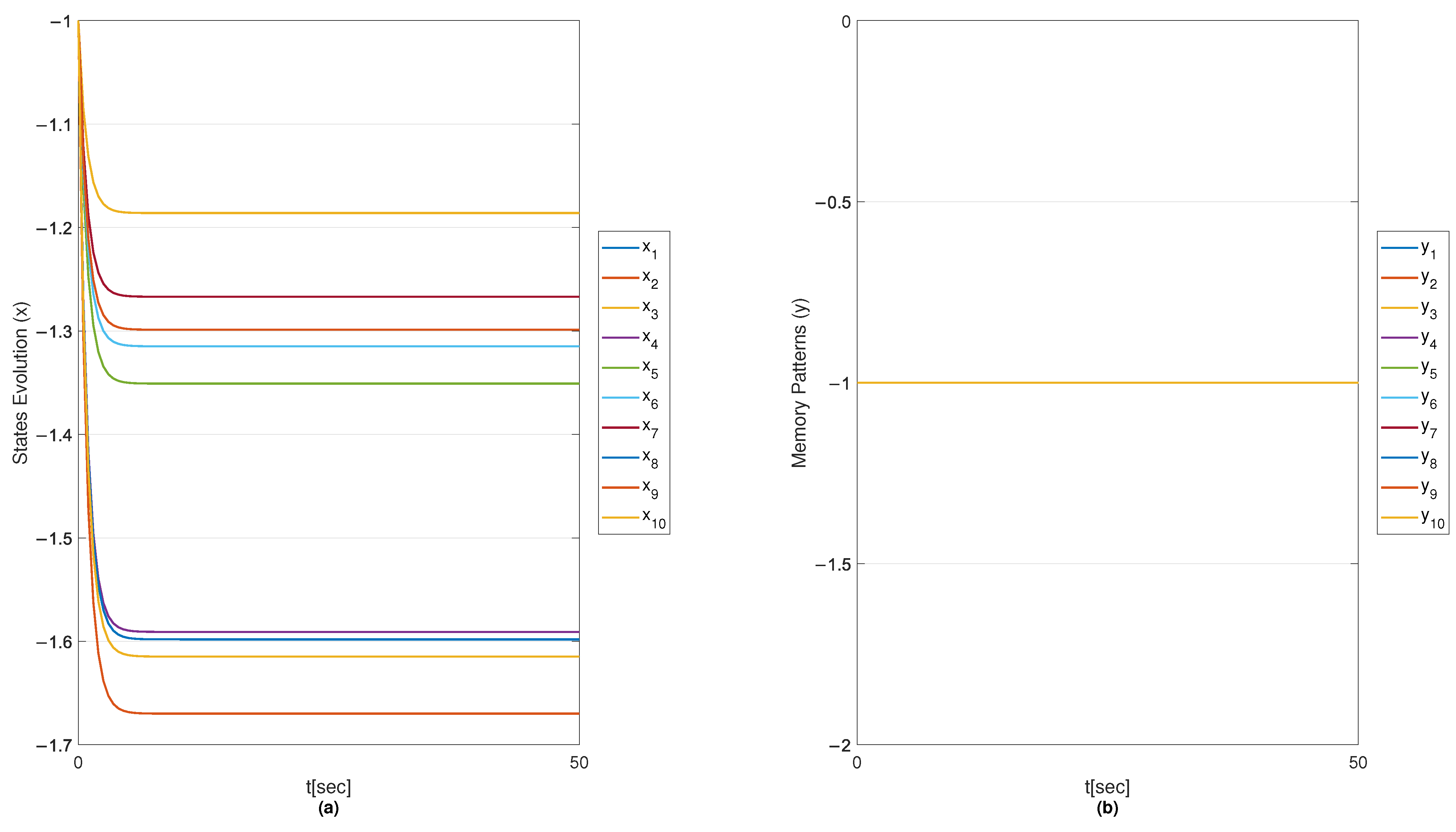
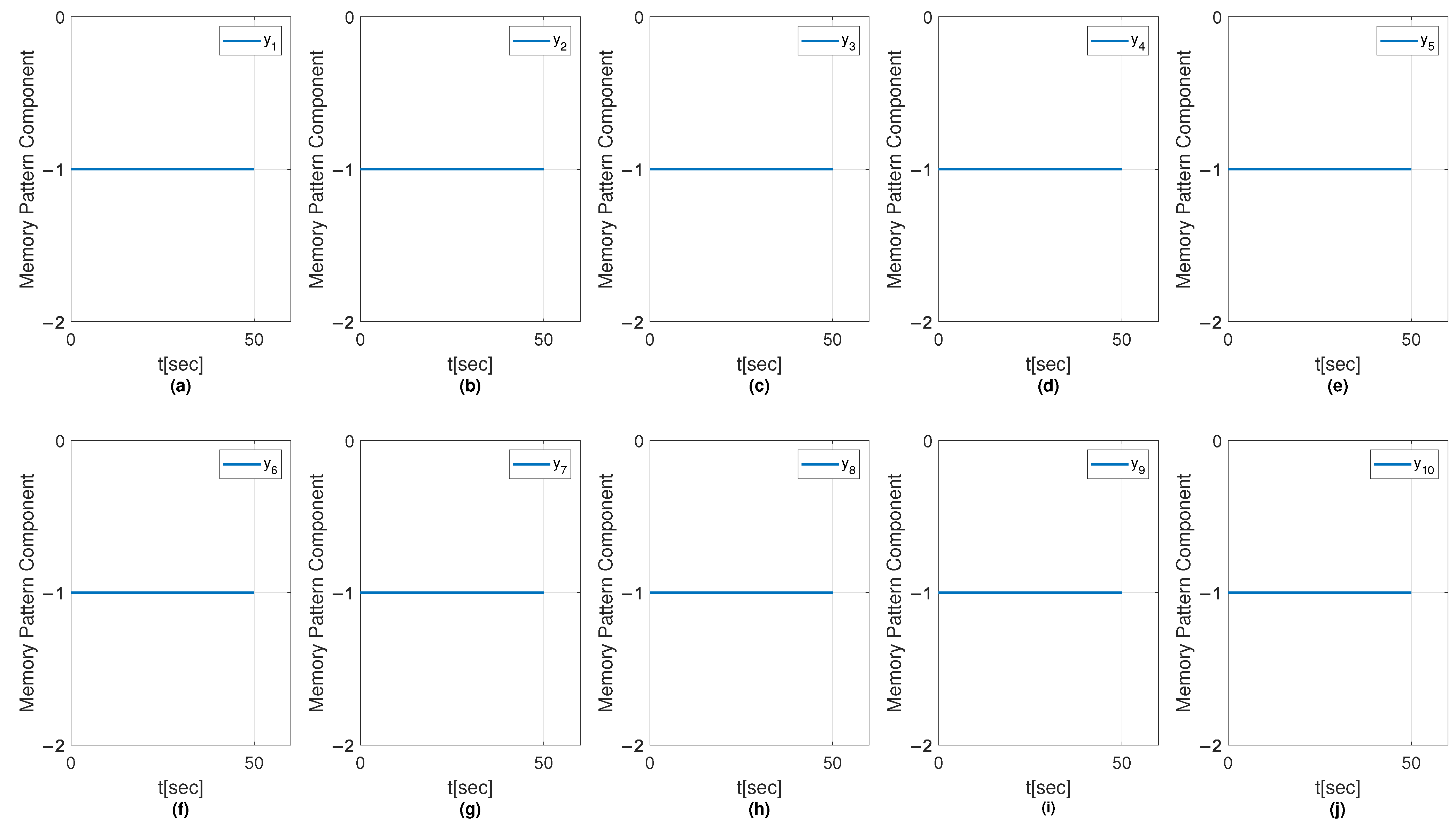
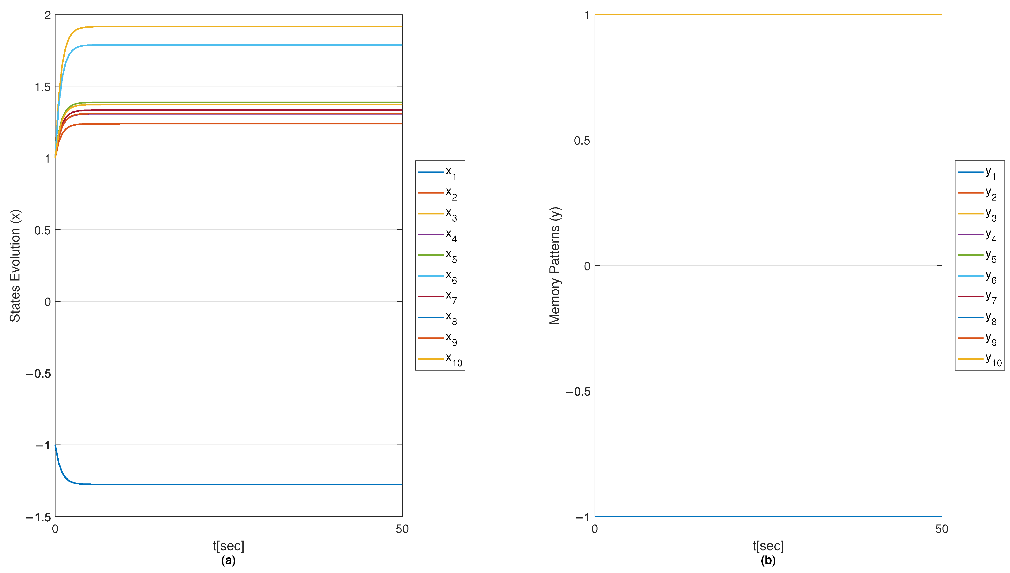
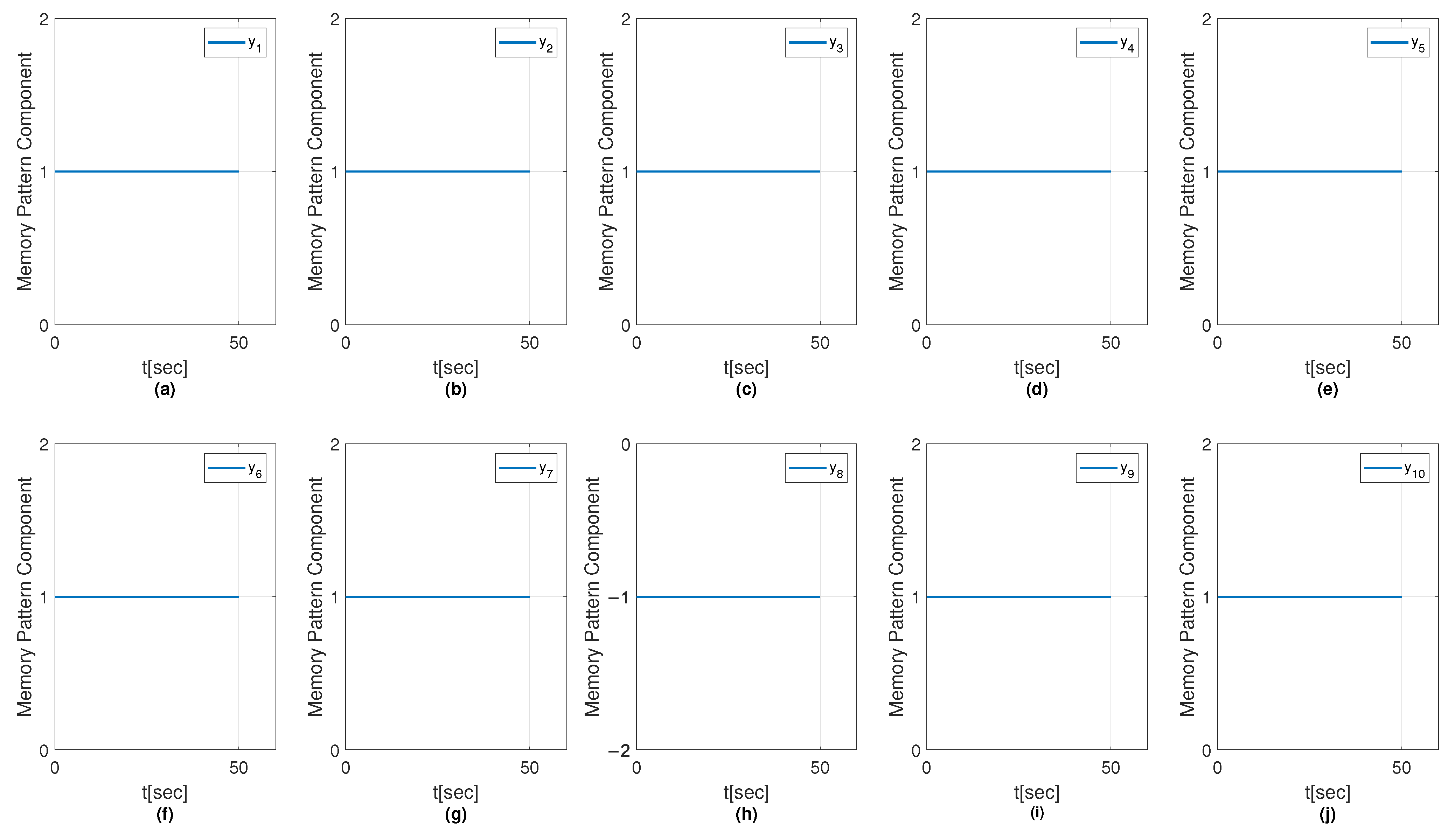
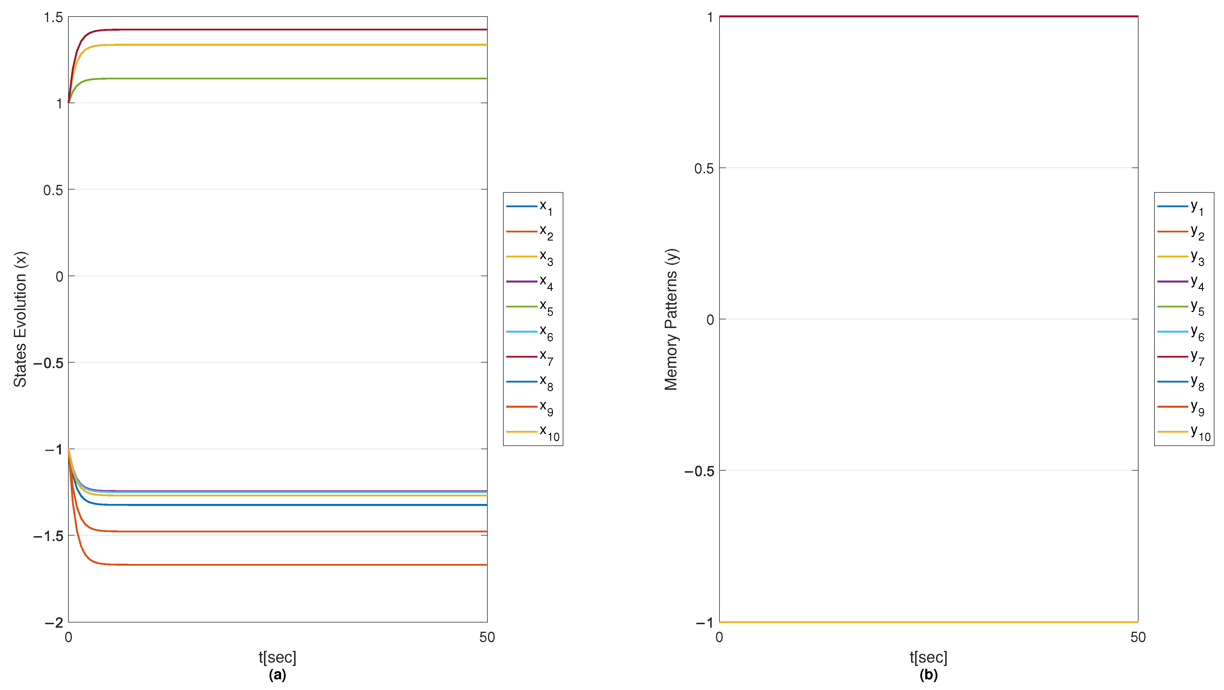
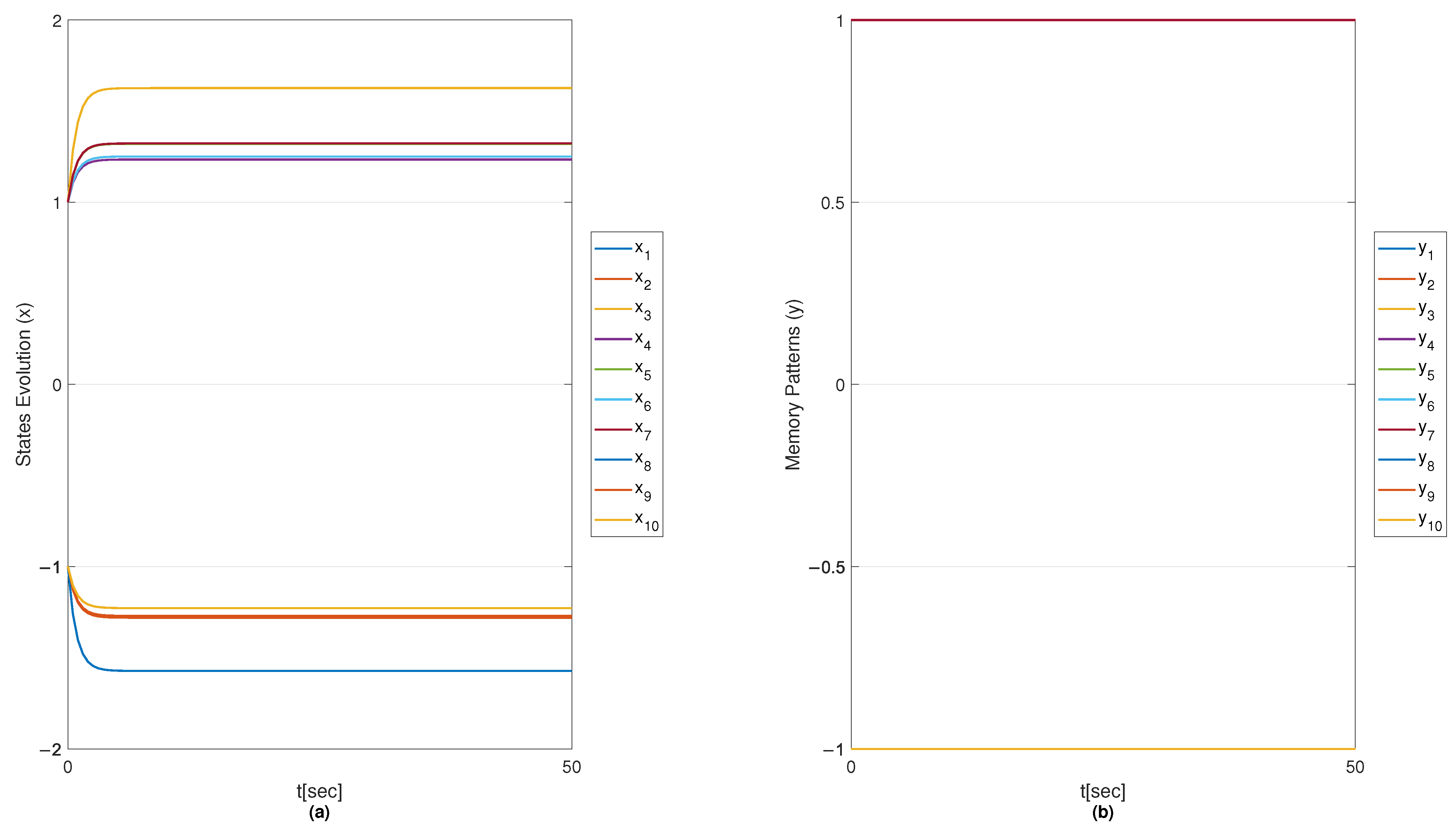
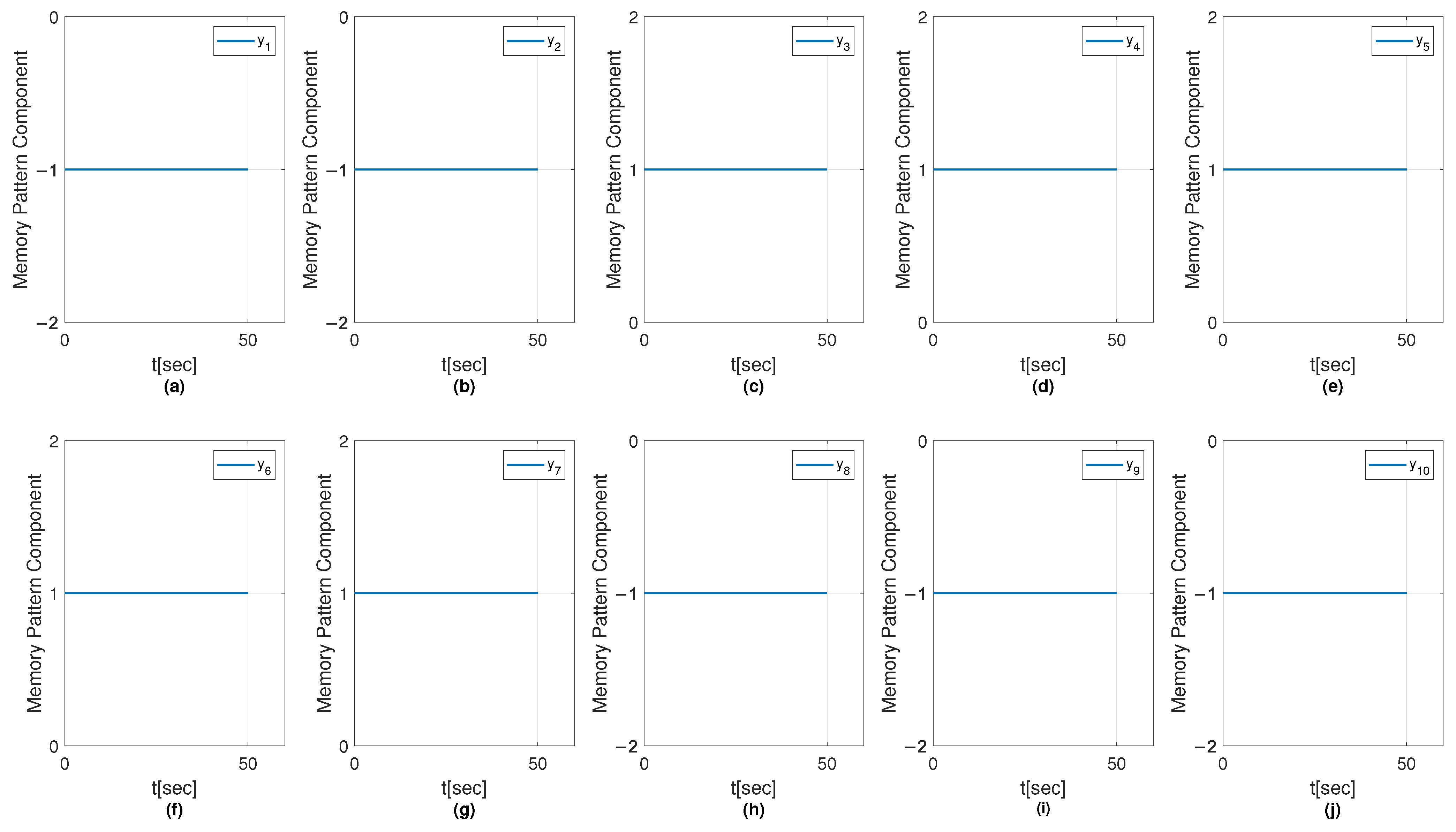
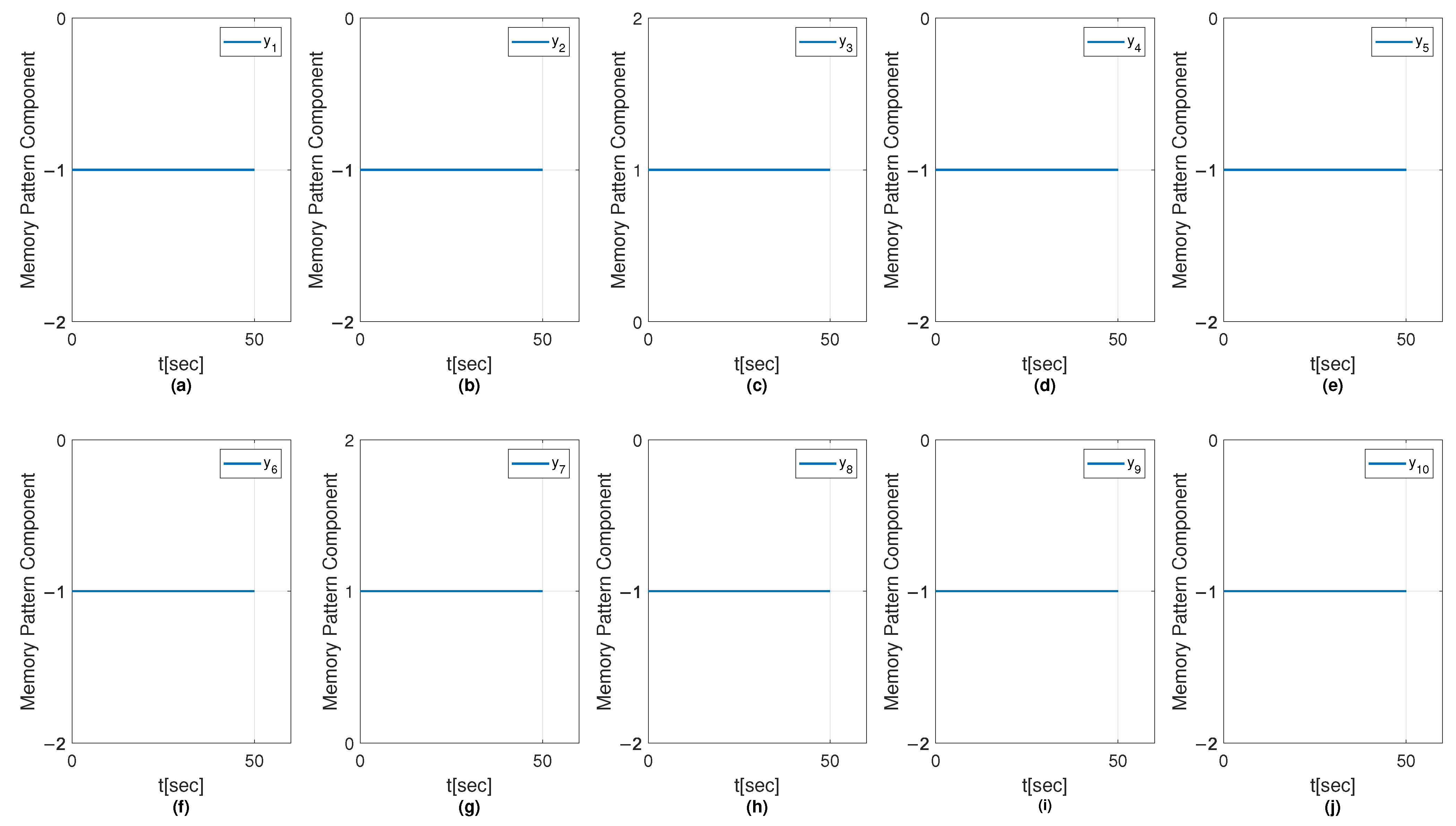
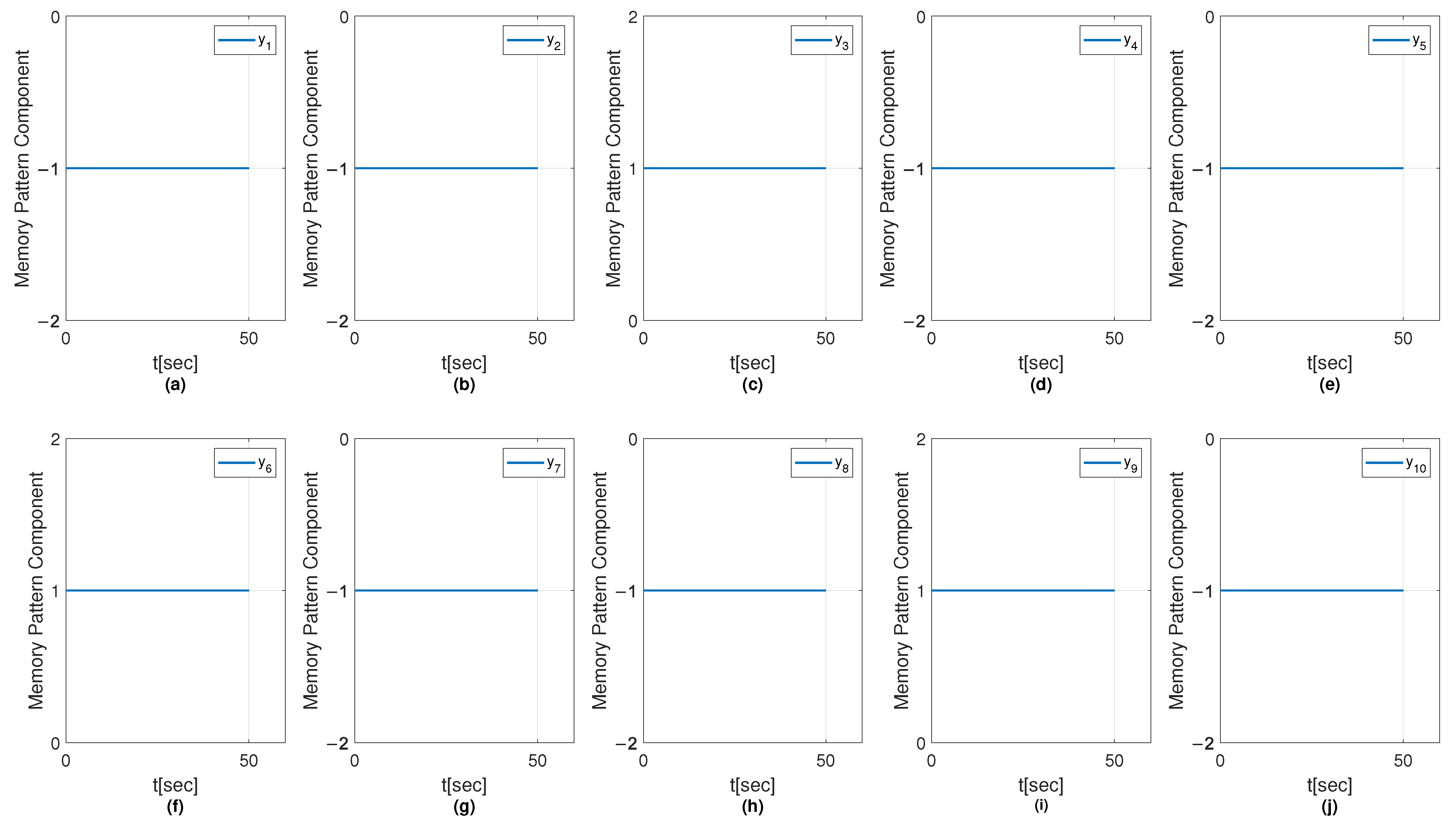
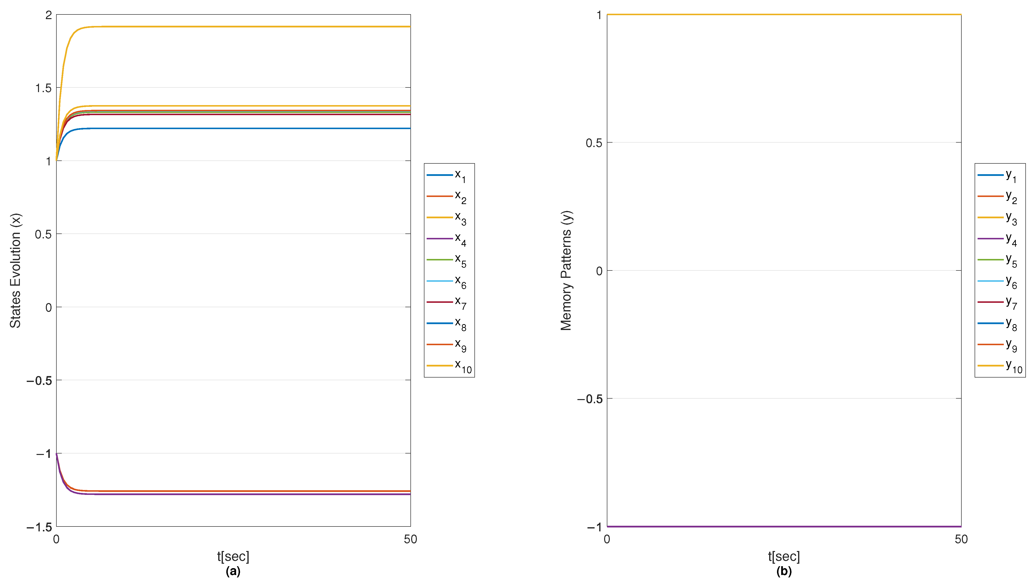
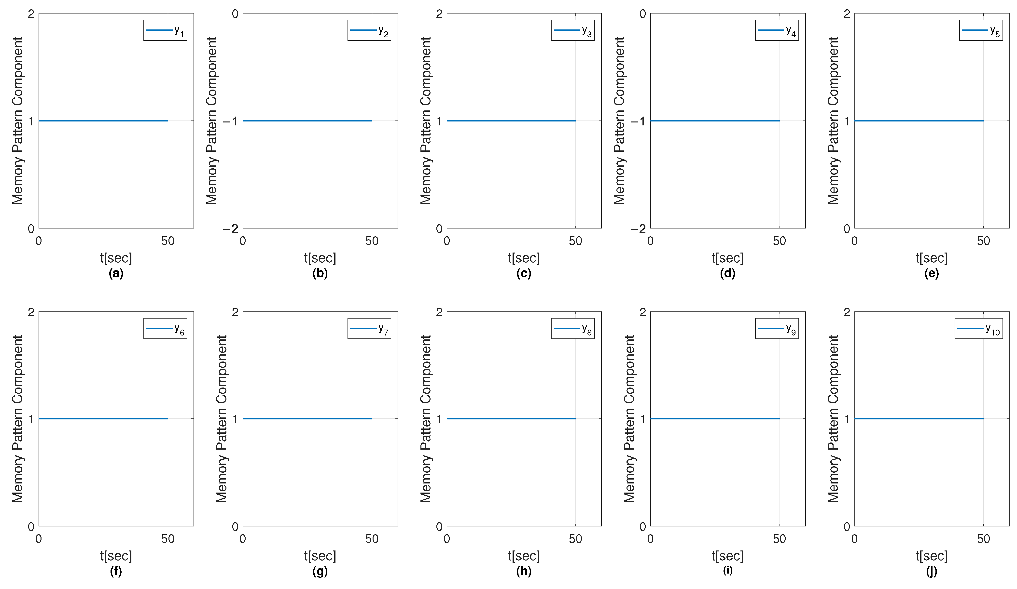
These results indicate that the main difference between the obtained matrices and the training algorithm is the connection matrix T, specifically its diagonal, and the I matrix. After the NAM has been trained, the results are presented in Figure 15, Figure 16, Figure 17, Figure 18, Figure 19, Figure 20, Figure 21, Figure 22, Figure 23, Figure 24, Figure 25, Figure 26, Figure 27 and Figure 28 which cover both the state evolution of the NAM and the corresponding component outputs. In particular, Figure 15, Figure 17, Figure 19, Figure 21, Figure 23, Figure 25 and Figure 27 show the retrieved pattern response for the seven faults, where subfigure (a) illustrates the state evolution of x, demonstrating a clear convergent behavior toward the equivalent of each stored fault pattern, and subfigure (b) presents the output of y from Equation (22). Complementarily, Figure 16, Figure 18, Figure 20, Figure 22, Figure 24, Figure 26 and Figure 28 depict the outputs of components $y_1$ to $y_{10}$ associated with each retrieved fault pattern.

6.2. Convergence Analysis

To increase the reliability of the obtained results and to further show improvement of the MSMOH algorithm, a convergence analysis is conducted. Hopfield networks, such as the NAM used in this study, can generate spurious memories, which are stable memories which are not desired and are not part of the fault patterns used for training. Consequently, testing the NAM with different training algorithms allowed for a through evaluation of its performance with all $2^{10}$ possible input combinations $\left(1024\mathrm{elements}\right)$.

Results for the number of convergent, non-convergent, and spurious elements for each training algorithm are presented in

Table 16. Convergence analysis with all training algorithms.

Training Algorithm	Number of Convergent Elements	Number of Not Convergent Elements	Spurious Memories	$\mathit{\mu }$	C	A
Perceptron	991	33	22	7	-	1
OH	797	227	9	1.6486	-	1.22
SMOH	780	244	11	1.6486	0.6322	1.22
MSMOH	1019	5	2	1.6486	0.6322	1.22

where MSMOH has the smallest number of spurious memories $\left(2\right)$ and has the highest number of elements that converged to one of stored patterns $\left(1019\right)$. This provides strong evidence that MSMOH is superior to the other three methods for retrieving stored fault patterns.

7. Discussion

This paper introduces a modified optimal hyperplane for SVM, termed MSMOH, which shows significant advantages over the conventional SMOH. These advantages include a reduction in the number of SVs and a wider maximization of the hyperplane’s margin. Classification task have been carried out using synthetic data as a visual tool of hyperplane construction, and real heart disease diagnoses have also been conducted with great results. In Section 5.1, the first approach to the performance of MSMOH classification demonstrated good results, the capacity to reduce the number of SVs, and an increase in the margin, where, in the MSMOH classification, the margin is $d=0.7992$ and the number of SVs is 14 out of 200 possible data inputs. In contrast, SMOH required 171 SVs from the same data input to obtain a margin $d=0.4037$, while its performance metrics were the worst. Figure 4 and Figure 5 illustrate hyperplane construction for both methods, with their respective subplots (a), (b), and (c) detailing their respective visual representations (SVs, margin, and data points). Furthermore, as shown in Table 3, the MSMOH method demonstrated a significantly lower average computational cost during the training process compared to SMOH.

In Section 5.2.2 Table 8 is presented with the MSMOH for SVM implemented in heart disease classification without considering validation at all, only prediction of all labeled data of the heart disease database. However, this study allows the measurement of the performance with a larger amount of data. In this case, the accuracy obtained with MSMOH is over-passed by that with SMOH, meaning that it has a higher proportion of correct predictions related to the labeled data. On the other hand, specificity and precision are better in MSMOH, where specificity indicates that this model has a better performance to identify negative instances out of all negative instances. F1 score is the result of precision and sensitivity, and despite the differences between the MSMOH and SMOH, the F1 score is slightly lower in MSMOH compared to SMOH. The most important part is the number of SVs needed to construct the hyperplane, with MSMOH using less and generating a wider margin.

In Section 5.2.3 cross-validation is carried out and this allows comparison between training results and test results. In this case, cross-validation helps to acquire a better understanding of the performance of MSMOH and SMOH considering different combinations of folds to train and test the model. MSMOH has a similar average performance in training (Table 9) and testing (Table 10) with a similar number of SVs considered in hyperplane construction, which also gives an average margin in all cases where these results are supported with the average, standard deviation, and MAGG of each metric performance. SMOH illustrates the cross-validation performance in testing (Table 11) and training (Table 12) where the same metrics have been calculated. MAGGs have been calculated to demonstrate the generalization capacity of MSMOH and SMOH, where MSMOH gives a better generalization with MAGG $=0.3092$ while SMOH gives a MAGG $=1.1070$ as presented in Table 13.

Moreover, the new MSMOH considering $p=2$ has been employed to train a NAM in Section 6 where results have been compared to other training algorithms where the main problems are related to a high number of spurious memories. However, MSMOH has better performance in comparison with perceptron, OH, and SMOH training due to 1019 possible input elements converging to one of the 7 stored fault patterns and only 5 possible input elements converging to one of the 2 spurious memories as illustrated in Table 16. NAM trained with MSMOH can thus be used for retrieving digit patterns by leveraging its ability to recall memories form a corrupted or incomplete image. It does this by converging to a stored digit pattern that is closest to the input, which provides advantages as presented in this study.

From the perspective of symmetry and asymmetry in classification tasks, the proposed MSMOH formulation aims to construct decision boundaries that maintain a balanced separation between classes, even when the underlying data distribution is asymmetric in terms of class size, feature variance, or SVs distribution. In symmetric scenarios, the hyperplane remains equidistant from the nearest elements of each class, whereas in asymmetric cases, conventional SMOH often shifts the boundary towards the more compact class. By prioritizing the penalization of large misclassification errors, MSOH reduces this bias, achieving a more symmetric margin distribution.

Furthermore, in the context of NAM training, this balanced separation improves the matching rate defined as the accurate convergence of noisy or incomplete input patterns to their corresponding stored patterns while decreasing unmatching occurrences, which include convergence to incorrect patterns or spurious memories. This improvement is particularly relevant in fault diagnosis and disease detection applications, where high matching accuracy under asymmetric and noisy conditions is critical.

Beyond power plants, fault detection is a significant challenge in other areas, such as automation processes and fault-tolerant control systems. For example, a key application is bearing fault diagnosis, where a NAM can be trained to identify and classify defects or malfunctions in rolling element bearings using vibration analysis and other techniques. Ultimately, early detection of faults is crucial for preventing catastrophic failures and minimizing downtime.

8. Conclusions

In conclusion, the results obtained show an improvement in NAM training with the MSMOH applied to fault diagnosis in fossil power plants, with the number of spurious memories being smaller compared to perceptron, OH, and SMOH. This could mean that if more patterns needs to be learn, the MSMOH would reduce the risk of false memories ensuring that the solutions are optimal only for the stored patterns. Furthermore, it is worth mentioning that the obtained results do not consider “optimal restrictions” as described in [17,19] which are limited for perceptron and OH training; this optimal restrictions allows manipulation of the diagonal elements of the connection matrix T when optimal conditions are obtained during NAM training.

These limitations encourage authors to extensively analyze and propose the possible “optimal restrictions” that could be applied for the SMOH and MSMOH in future work including application in other topics (e.g., digit reconstruction, bearing fault diagnosis, and fault tolerant control, among others) where there are more patterns or a larger number of elements are needed to be stored while contributing to advances in non-supervised learning models such as NAM.

On the other hand, the MSMOH algorithms are currently in development to work with alternative methods such as evolutionary algorithms that will allow for searching for optimal values that could improve classification including values of $p>1$ reducing the limitations of case where $p=2$ and the QP solving for the hyperplane construction. Moreover, not only working with linear kernels but also with polynomial and Gaussian ones, including the search of hyperparameters within the hyperplane construction, are avenues for future work. In addition, MSMOH could be compared to broader classification methods and additional performance metrics that allow an extensive validation of MSMOH’s advantages over SMOH.

References

1. Abe, S. Support Vector Machines for Pattern Classification; Springer: Berlin/Heidelberg, Germany, 2005; Volume 2. [Google Scholar]
2. Chandra, M.A.; Bedi, S. Survey on SVM and their application in image classification. Int. J. Inf. Technol. 2021, 13, 1–11. [Google Scholar] [CrossRef]
3. Lo, C.S.; Wang, C.M. Support vector machine for breast MR image classification. Comput. Math. Appl. 2012, 64, 1153–1162. [Google Scholar] [CrossRef]
4. Homaeinezhad, M.; Tavakkoli, E.; Atyabi, S.; Ghaffari, A.; Ebrahimpour, R. Synthesis of multiple-type classification algorithms for robust heart rhythm type recognition: Neuro-svm-pnn learning machine with virtual QRS image-based geometrical features. Sci. Iran. 2011, 18, 423–431. [Google Scholar] [CrossRef]
5. Bansal, M.; Goyal, A.; Choudhary, A. A comparative analysis of K-nearest neighbor, genetic, support vector machine, decision tree, and long short term memory algorithms in machine learning. Decis. Anal. J. 2022, 3, 100071. [Google Scholar] [CrossRef]
6. Cortes, C.; Vapnik, V. Support-vector networks. Mach. Learn. 1995, 20, 273–297. [Google Scholar] [CrossRef]
7. Zhang, H.; Shi, Y.; Yang, X.; Zhou, R. A firefly algorithm modified support vector machine for the credit risk assessment of supply chain finance. Res. Int. Bus. Financ. 2021, 58, 101482. [Google Scholar] [CrossRef]
8. Meng, E.; Huang, S.; Huang, Q.; Fang, W.; Wang, H.; Leng, G.; Wang, L.; Liang, H. A hybrid VMD-SVM model for practical streamflow prediction using an innovative input selection framework. Water Resour. Manag. 2021, 35, 1321–1337. [Google Scholar] [CrossRef]
9. Divya, P.; Devi, B.A. Hybrid metaheuristic algorithm enhanced support vector machine for epileptic seizure detection. Biomed. Signal Process. Control 2022, 78, 103841. [Google Scholar] [CrossRef]
10. Laxmi, S.; Gupta, S.; Kumar, S. Intuitionistic fuzzy least square twin support vector machines for pattern classification. Ann. Oper. Res. 2024, 339, 1329–1378. [Google Scholar] [CrossRef]
11. Wang, H. A novel feature selection method based on quantum support vector machine. Phys. Scr. 2024, 99, 056006. [Google Scholar] [CrossRef]
12. Gao, Z.; Cecati, C.; Ding, S.X. A Survey of Fault Diagnosis and Fault-Tolerant Techniques—Part I: Fault Diagnosis With Model-Based and Signal-Based Approaches. IEEE Trans. Ind. Electron. 2015, 62, 3757–3767. [Google Scholar] [CrossRef]
13. Van Schrick, D. Remarks on terminology in the field of supervision, fault detection and diagnosis. IFAC Proc. Vol. 1997, 30, 959–964. [Google Scholar] [CrossRef]
14. Çira, F.; Arkan, M.; Gümüş, B. A new approach to detect stator fault in permanent magnet synchronous motors. In Proceedings of the 2015 IEEE 10th International Symposium on Diagnostics for Electrical Machines, Power Electronics and Drives (SDEMPED), Guarda, Portugal, 1–4 September 2015; pp. 316–321. [Google Scholar] [CrossRef]
15. Li, Y.; Zhang, Y.; Liu, W.; Chen, Z.; Li, Y.; Yang, J. A Fault Pattern and Convolutional Neural Network Based Single-phase Earth Fault Identification Method for Distribution Network. In Proceedings of the 2019 IEEE Innovative Smart Grid Technologies—Asia (ISGT Asia), Chengdu, China, 21–24 May 2019; pp. 838–843. [Google Scholar] [CrossRef]
16. Vapnik, V. Statistical Learning Theory; John Wiley and Sons: Hoboken, NJ, USA, 1998. [Google Scholar]
17. Ruz-Hernandez, J.A.; Suarez, D.A.; Garcia-Hernandez, R.; Sanchez, E.N.; Suarez-Duran, M.U. Optimal training algorithm application to design an associative memory for fault diagnosis at a fossil electric power plant. IFAC Proc. Vol. 2012, 45, 756–762. [Google Scholar] [CrossRef]
18. Ruz-Hernandez, J.A.; Sanchez, E.N.; Suarez, D.A. Soft Margin Training for Associative Memories: Application to Fault Diagnosis in Fossil Electric Power Plants. In Soft Computing for Hybrid Intelligent Systems; Springer: Berlin/Heidelberg, Germany, 2008; pp. 205–230. [Google Scholar] [CrossRef]
19. Liu, D.; Lu, Z. A new synthesis approach for feedback neural networks based on the perceptron training algorithm. IEEE Trans. Neural Netw. 1997, 8, 1468–1482. [Google Scholar] [CrossRef] [PubMed]
20. dos Santos, A.S.; Valle, M.E. Max-C and Min-D Projection Auto-Associative Fuzzy Morphological Memories: Theory and an Application for Face Recognition. Appl. Math. 2023, 3, 989–1018. [Google Scholar] [CrossRef]
21. Janosi, A.; Steinbrunn, W.; Pfisterer, M.; Detrano, R. Heart Disease Data Set. 1989. Available online: https://archive.ics.uci.edu/ml/datasets/heart+Disease (accessed on 1 July 2025).
22. Pedregosa, F.; Varoquaux, G.; Gramfort, A.; Michel, V.; Thirion, B.; Grisel, O.; Blondel, M.; Prettenhofer, P.; Weiss, R.; Dubourg, V.; et al. Scikit-learn: Machine Learning in Python. J. Mach. Learn. Res. 2011, 12, 2825–2830. [Google Scholar]
23. Ruz-Hernandez, J.A.; Sanchez, E.N.; Suarez, D.A. Fault Detection and Diagnosis for Fossil Electric Power Plants via Recurrent Neural Networks. Dyn. Continous Discret. Impuls. Syst. Ser. B 2008, 15, 219. [Google Scholar]
24. Aoki, M. Introduction to Optimization Techniques: Fundamentals and Applications of Nonlinear Programming; Macmillan: New York, NY, USA, 1971. [Google Scholar]
25. Haykin, S. Neural Networks: A Comprehensive Foundation, 2nd ed.; Prentice Hall: Hoboken, NJ, USA, 1999. [Google Scholar]
26. Vapnik, V. The Nature of Statistical Learning Theory; Springer Science & Business Media: Berlin/Heidelberg, Germany, 2000. [Google Scholar] [CrossRef]
Figure 1. Soft margin optimal hyperplane with examples of ξ = 0 , ξ > 1 , and ξ < 1 .
Symmetry 17 01749 g001
Figure 2. ξ effect on ξ σ function.
Symmetry 17 01749 g002
Figure 3. Synthetic data.
Symmetry 17 01749 g003
Figure 4. (a) Classification of synthetic data with MSMOH; (b) zoom of the classification of margin with MSMOH; (c) the MSMOH constructed and the SVs used for the construction.
Symmetry 17 01749 g004
Figure 5. (a) Classification of synthetic data with SMOH; (b) zoom of the classification of margin with SMOH; (c) the SMOH constructed and the SVs used for the construction.
Symmetry 17 01749 g005
Figure 6. Correlation matrix of the heart disease database.
Symmetry 17 01749 g006
Figure 7. Confusion matrix with SVM-MSMOH classification.
Symmetry 17 01749 g007
Figure 8. Confusion matrix with SVM-SMOH classification.
Symmetry 17 01749 g008
Figure 9. Confusion matrix with SVM-MSMOH with cross-validation classification. (a) First validation, (b) second validation, (c) third validation, (d) fourth validation, and (e) fifth validation.
Symmetry 17 01749 g009
Figure 10. ROC curve of cross-validation with SVM-MSMOH. (a) First validation, (b) second validation, (c) third validation, (d) fourth validation, and (e) fifth validation.
Symmetry 17 01749 g010
Figure 11. Confusion matrix with SVM-SMOH with cross-validation classification. (a) First validation, (b) second validation, (c) third validation, (d) fourth validation, and (e) fifth validation.
Symmetry 17 01749 g011
Figure 12. ROC curve of cross-validation with SVM-SMOH. (a) First validation, (b) second validation, (c) third validation, (d) fourth validation, and (e) fifth validation.
Symmetry 17 01749 g012
Figure 13. Fault diagnosis scheme.
Symmetry 17 01749 g013
Figure 14. Fault classification scheme.
Symmetry 17 01749 g014
Figure 15. Retrieving of fault pattern ( F 0 ) . (a) States evolution; (b) fault pattern retrieved.
Symmetry 17 01749 g015
Figure 16. Output of NAM obtained for each state x with y = s a t ( x ) defined in (22). Figures (aj) describe the output obtained from y 1 to y 10 elements of the ( F 0 ) fault pattern retrieved.
Symmetry 17 01749 g016
Figure 17. Retrieving of Fault Pattern 1 ( F 1 ) . (a) States evolution; (b) fault pattern retrieved.
Symmetry 17 01749 g017
Figure 18. Output of NAM obtained for each state x with y = s a t ( x ) defined in (22). Figures (aj) describe the output obtained from y 1 to y 10 elements of the ( F 1 ) fault pattern retrieved.
Symmetry 17 01749 g018
Figure 19. Retrieving of Fault Pattern 2 ( F 2 ) . (a) States evolution; (b) fault pattern retrieved.
Symmetry 17 01749 g019
Figure 20. Output of NAM obtained for each state x with y = s a t ( x ) defined in (22). Figures (aj) describe the output obtained from y 1 to y 10 elements of the ( F 2 ) fault pattern retrieved.
Symmetry 17 01749 g020
Figure 21. Retrieving of Fault Pattern 3 ( F 3 ) . (a) States evolution; (b) fault pattern retrieved.
Symmetry 17 01749 g021
Figure 22. Output of NAM obtained for each state x with y = s a t ( x ) defined in (22). Figures (aj) describe the output obtained from y 1 to y 10 elements of the ( F 3 ) fault pattern retrieved.
Symmetry 17 01749 g022
Figure 23. Retrieving of Fault Pattern 4 ( F 4 ) . (a) States evolution; (b) fault pattern retrieved.
Symmetry 17 01749 g023
Figure 24. Output of NAM obtained for each state x with y = s a t ( x ) defined in (22). Figures (aj) describe the output obtained from y 1 to y 10 elements of the ( F 4 ) fault pattern retrieved.
Symmetry 17 01749 g024
Figure 25. Retrieving of Fault Pattern 5 ( F 5 ) . (a) States evolution; (b) fault pattern retrieved.
Symmetry 17 01749 g025
Figure 26. Output of NAM obtained for each state x with y = s a t ( x ) defined in (22). Figures (aj) describe the output obtained from y 1 to y 10 elements of the ( F 5 ) fault pattern retrieved.
Symmetry 17 01749 g026
Figure 27. Retrieving of Fault Pattern 6 ( F 6 ) . (a) States evolution; (b) fault pattern retrieved.
Symmetry 17 01749 g027
Figure 28. Output of NAM obtained for each state x with y = s a t ( x ) defined in (22). Figures (aj) describe the output obtained from y 1 to y 10 elements of the ( F 6 ) fault pattern retrieved.
Symmetry 17 01749 g028