1. Introduction
Mobile mapping systems are increasingly utilizing Multi-LiDAR platforms because they reduce occlusions and improve geometric stability and point cloud completeness [
1,
2,
3,
4,
5]. The performance of Multi-LiDAR systems largely depends on sensor quality and configuration factors such as orientation, placement, and field of view (FOV) [
4,
5,
6,
7,
8]. Improperly configured LiDARs can result in excessive blind spots, poor registration overlap, limited angular diversity, or inefficient redundancy, all of which will negatively impact mapping reliability.
The design of LiDAR configuration systems is inherently complex due to the highly anisotropic sampling pattern produced by a spinning LiDAR. This is primarily influenced by the vertical-channel configuration, the azimuth-resolving capability, and beam divergence [
6,
9,
10]. The combination of multiple LiDARs leads to nonlinear interactions because visibility patterns are affected by sensor orientations, platform motion, occlusion geometries, and the alignment of coordinate frames. Consequently, the combination of these parameters creates a high-dimensional non-convex optimization problem that cannot be solved analytically. This complex problem of LiDAR configuration design has led us to develop black-box optimization methods that do not require analytical gradients and can directly optimize coverage metrics derived from physical coverage simulations.
Previous studies have mainly relied on heuristic rules or manual tuning to solve the design problem of LiDAR configurations [
6,
11,
12,
13]. These earlier methods cannot systematically examine all possible configurations and often produce suboptimal or inconsistent designs. More recent studies indicate that the placement of LiDAR sensors greatly impacts point cloud coverage, the reduction in blind zones, geometric data redundancy, and overall perception performance [
7,
8,
13,
14,
15]. For applications in autonomous driving and infrastructure sensing, multi-LiDAR configurations have been explored through occupancy-grid mapping, simulation, and perception-based criteria, showing that sensor placement and orientation significantly affect point density, uniformity, and system performance. However, many current methods depend on predefined candidate locations, simplified sensor models, or application-specific metrics, which do not fully solve the mixed discrete–continuous mount-design problem in compact mobile mapping systems. In these systems, the number, position, and orientation of sensors need to be optimized concurrently. This highlights the need for a physically grounded optimization framework that jointly considers sensor count, placement, and orientation while respecting practical symmetry and clearance constraints.
Advances in algorithmic optimization and computational intelligence enable the formalization of the configuration problem and the identification of optimal sensor positions through automated, principled approaches. This paper examines the optimization of multi-LiDAR setups under symmetry constraints, which are common in commercial backpack and handheld mapping systems.
This paper investigates how to mathematically optimize multi-LiDAR configurations subject to symmetry constraints. Three algorithmic approaches are examined.
Bayesian Optimization (BO): A surrogate-based method using Gaussian Processes to model the costly black-box objective and direct the search through expected improvement [
16,
17].
Genetic Algorithms (GA): An evolutionary strategy that maintains population diversity and performs global exploration through crossover and mutation [
18,
19].
Particle Swarm Optimization (PSO): A computational intelligence method in which particles adapt their velocities based on cognitive and social learning components [
20,
21].
BO, GA, and PSO each have their own strengths: BO is effective for costly evaluations, GA explores complex high-dimensional spaces using population diversity, and PSO rapidly converges in smooth regions of the landscape. Since the multi-LiDAR configuration problem is nonconvex and contains both smooth and irregular areas, using all three algorithms ensures robustness and prevents reliance on any single optimizer’s assumptions.
The choice of BO, GA, and PSO in this study aims to represent three distinct families of optimizers rather than cover the entire range of available methods. BO represents sample-efficient, surrogate-based optimization suitable for costly black-box functions; GA reflects evolutionary, population-based methods for global search in multimodal landscapes; and PSO represents swarm-oriented, continuous search with unique convergence behaviors. Given that the multi-LiDAR configuration problem involves mixed discrete–continuous variables, nonconvexity, and expensive evaluations, these three approaches offer a valuable cross-section of methodologies. They are used to determine whether stable, structural solutions remain consistent across fundamentally different optimization strategies. The aim is not to rank all optimizers but to evaluate the structural robustness of the solutions found across the search paradigms of these representative techniques.
To evaluate candidate configurations, we develop a voxel-level LiDAR simulation pipeline that accurately models real-sensor behavior, including channel geometry, azimuthal rotation, occlusion-aware ray casting, and beam divergence [
9,
10,
13,
14]. The evaluation metric combines (i) unique voxel coverage, (ii) overlap ratio within a target range, and (iii) inter-sensor angular diversity, together providing a comprehensive measure of quality for multi-LiDAR mapping.
In mobile mapping and downstream SLAM, these three criteria serve distinct but complementary functions [
4,
5,
12,
13]. Coverage improves scene observability by reducing blind spots along the trajectory. Overlap provides shared visibility, which is essential for inter-sensor registration and ensuring scan-to-scan consistency. Angular diversity enhances geometric conditioning by minimizing near-parallel viewing angles and lowering scan-matching degeneracy [
6,
7,
12,
13]. In this study, these factors are regarded as geometric proxy indicators of mapping quality rather than direct SLAM performance metrics, since a comprehensive SLAM benchmark is outside the current scope.
The main innovative aspects of this study are:
A physically grounded mixed discrete–continuous optimization framework for designing symmetric multi-LiDAR mounts under mechanical constraints.
A voxel-accurate simulation and evaluation pipeline that simultaneously models coverage, overlap, and angular diversity for spinning LiDAR systems.
A comparative cross-optimizer analysis demonstrates that structurally consistent symmetric dual-sensor configurations emerge consistently in BO, GA, and PSO methods.
A post-optimization validation shows that configurations found in a simplified environment maintain their geometric effectiveness in a more realistic indoor scene.
The key innovation of this study lies not in introducing a new optimizer but in formulating the multi-LiDAR-mount design as a physically grounded mixed discrete–continuous optimization problem. The proposed approach can simultaneously determine the number of sensors, their coordinates, and their orientations, while accounting for sensor symmetry and any existing mechanical limitations. As mentioned, previous LiDAR configuration research relied on predetermined candidate locations, heuristic modifications to the design process, or simplified coverage models. The proposed method is built around a combination of voxel-accurate LiDAR simulation and appropriately designed reward functions. This method reveals structural optimization that is stable and repeatable across a variety of types of optimizers. This is why the contribution of this work is both methodological and geometric, and it presents a new solution to the multi-LiDAR system design problem.
Accordingly, the following research questions are considered:
RQ1: Does the mixed discrete–continuous formulation converge to structurally consistent multi-LiDAR configurations across different optimization methods (BO, GA, and PSO)?
RQ2: What trade-offs develop between coverage maximization, overlap control, and angular diversity under a physically grounded voxel-based objective?
RQ3: Do configurations optimized in a simplified voxelized environment retain their geometric effectiveness when tested against realistic surface-based ground-truth models?
The rest of this paper is organized as follows.
Section 2 reviews existing research on multi-LiDAR systems and optimization techniques.
Section 3 describes the methodological frameworks for Bayesian Optimization (BO), Genetic Algorithm (GA), and Particle Swarm Optimization (PSO).
Section 4 presents the simulation setup and experimental design.
Section 5 discusses the findings and answers to the research questions.
Section 6 summarizes the study and conclusions.
2. Literature Review
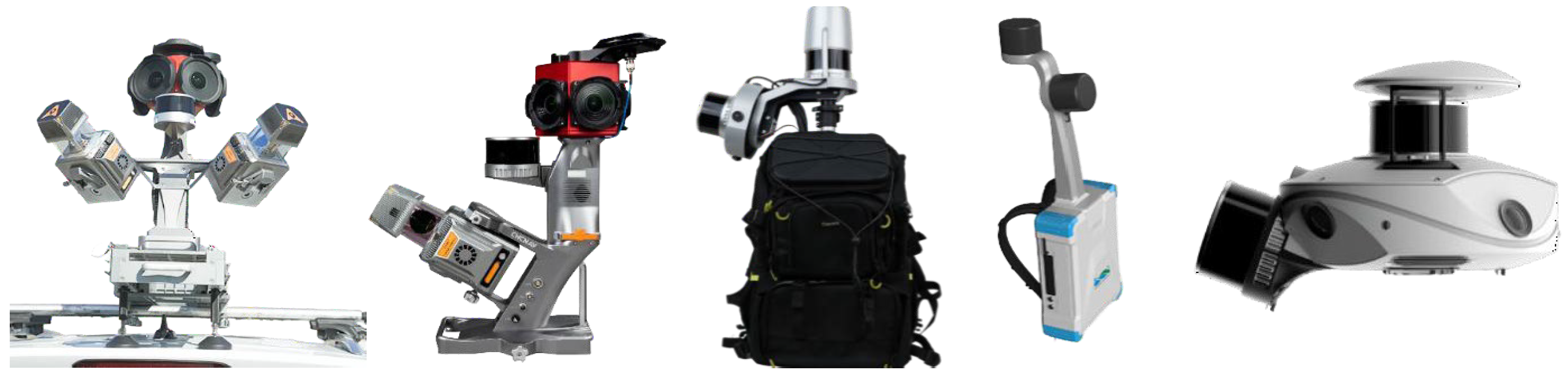
Modern mapping platforms increasingly combine multiple LiDAR sensors to minimize occlusions and enhance geometric data completeness. Commercial systems such as [
1,
2,
3] demonstrate the widespread use of dual- or multi-LiDAR configurations to achieve uniform scene coverage and stable calibration (
Figure 1). These products commonly exhibit bilateral symmetry, which motivates the symmetry constraint used in our framework.
Recent mobile-mapping research highlights the importance of comprehensive system design, calibration, and benchmarking for backpack and mobile laser-scanning platforms. For instance, the design and evaluation of backpack indoor mobile mapping have been explored within a dedicated system-level framework. Additionally, permanent test-field benchmarks have been employed to assess the geometric performance of mobile laser-scanning systems in real-world conditions. These studies demonstrate that multi-LiDAR configurations are not just a perception challenge but also a practical consideration in mobile-mapping system design [
4,
5].
Several studies have explored how orientation and configuration geometry influence LiDAR performance. Reference [
6] found that tilt angles between 30° and 45° offer a good balance between facade and ground visibility for 64-channel LiDARs, highlighting how sensitive coverage is to small changes in orientation. Research by ref. [
7] has shown that using diverse LiDAR orientations improves the robustness of 3D detection in autonomous driving. Similar results are observed in dual-LiDAR navigation systems, where fixed configurations improve heading estimation and reduce localization drift [
12]. These studies confirm that mount geometry significantly affects coverage, overlap, and angular diversity. However, they depend on manually chosen configurations rather than optimized solutions.
Increasing interest in automated sensor placement has led to the development of various deterministic and evolutionary approaches. Research by refs. [
8] and [
11] investigated the placement of multiple LiDARs on vehicles using geometric visibility and coverage criteria. Other studies proposed optimization strategies for roadside and UAV-LiDAR systems that utilize voxel modeling and occlusion analysis [
12,
13,
14]. While these methods highlight the benefits of formal optimization, they often depend on preset candidate poses, simplified LiDAR models, or purely deterministic search methods. So, they are restricting their capacity to navigate high-dimensional, continuous parameter spaces. Conversely, voxel-based ray-casting methods (e.g., refs. [
13,
14]) provide more physically accurate coverage evaluation, but lack adaptive optimization.
Overall, the literature shows that LiDAR configuration significantly affects coverage, redundancy, point cloud distribution, and perception quality. Past studies have provided valuable insights into multi-LiDAR placement, sensor deployment, and realistic LiDAR simulation. However, three key limitations remain relevant to the design of mobile mapping mounts. First, current methods apply optimization over predefined candidate locations rather than treating sensor position and orientation as continuous variables. Second, several approaches emphasize perception metrics, such as object detection or semantic segmentation, rather than general geometric mapping criteria [
7,
15]. Third, the potential of bilateral symmetry as a mechanical and geometric design prior has not been explicitly integrated into the optimization framework for backpack or compact mobile mapping systems. This study addresses these issues by integrating voxel-level LiDAR simulation, symmetry-constrained parameterization, and three popular black-box optimization strategies.
Previous multi-LiDAR placement techniques, whether deterministic, heuristic, or evolutionary, are often limited by the use of simplified LiDAR models, predetermined candidate poses, or single-objective techniques. This simplification results in coverage, overlap, and angular diversity being treated in isolation from one another, all of which limit the realism of the designs. Ultimately, they pose significant challenges to exploring the high-dimensional design space required for today’s multi-LiDAR systems. On the other hand, this research developed an integrated, physically based optimization framework for the automatic identification of symmetric multi-LiDAR configurations by applying various optimization techniques. The proposed framework combines voxel-level LiDAR simulation with joint optimization of coverage, overlap, and angular diversity, offering a scalable approach suitable for a range of mapping tasks and platforms. These gaps lead to a unified, data-driven optimization framework that includes:
- –
Physically accurate voxel-level LiDAR simulation;
- –
Symmetric mount parameterization;
- –
Global search using BO, GA, and PSO algorithms [
16,
17,
18,
19,
20,
21].
Our approach overcomes the limits of deterministic and heuristic methods by enabling automated exploration of the continuous configuration space while optimizing key geometric metrics. In addition to maximizing coverage, optimized multi-LiDAR setups can also affect observability and registration behavior. While these factors are important for downstream SLAM systems, their impacts are not directly evaluated in this study. By managing angular diversity and redundancy structure, the proposed framework supports perception-aware sensor system design rather than focusing solely on geometric placement optimization.
While these systems demonstrate the feasibility of multi-LiDAR setups, most rely on empirically determined mounts rather than optimization-based design solutions [
8,
11,
13]. The common use of bilateral symmetry (
Figure 1) not only simplifies integration and balance but also improves calibration stability. Along with mechanical balance, bilateral symmetry provides a structured geometric prior that regularizes the configuration space, maintains left–right observability balance, and facilitates repeatable calibration behavior. These insights motivate the explicit symmetry constraint used in our optimization framework (
Section 3).
3. Methodology
This paper proposes three optimization frameworks to solve the multi-LiDAR configuration problem introduced earlier. All three frameworks aim to automatically determine the optimal number, position, and orientation of LiDAR sensors to maximize coverage uniformity, minimize redundant overlap, and improve angular diversity within a physically valid, mechanically feasible design space. A physics-based LiDAR simulator performs voxel-level ray casting to evaluate the scanning performance of each configuration, modeling real-world characteristics such as beam divergence, vertical channel geometry, and full 360° azimuth rotation.
The first framework uses BO. This probabilistic global search method builds a surrogate model of the objective function and efficiently finds promising sensor configurations within a limited evaluation budget. The second framework uses GA to generate candidate LiDAR configurations via crossover and mutation, exploring the high-dimensional design space. The third framework uses PSO, in which particles continuously adjust their positions based on cognitive and social learning to find optimal configurations. Together, BO, GA, and PSO offer complementary global optimization methods: BO provides sample-efficient, surrogate-guided searches; GA encourages diversity for broad exploration; and PSO guarantees quick convergence on smooth, continuous problem surfaces. Because the multi-LiDAR configuration problem is highly nonconvex and admits multiple near-optimal solutions, different optimizers may converge to different sensor counts or orientations. This variability is not a flaw but reflects the natural complexity of the search landscape. The objective function penalizes unnecessary sensors and rewards coverage, overlap, and diversity in angular coverage. This will enable each optimizer to find the multi-LiDAR configuration that best balances these criteria within its own search process. Furthermore, comparing the three proposed optimization techniques of BO, GA, and PSO offers insights into the robustness of the solution space. It should confirm that conclusions are not based solely on any one method or algorithm.
3.1. Problem Definition
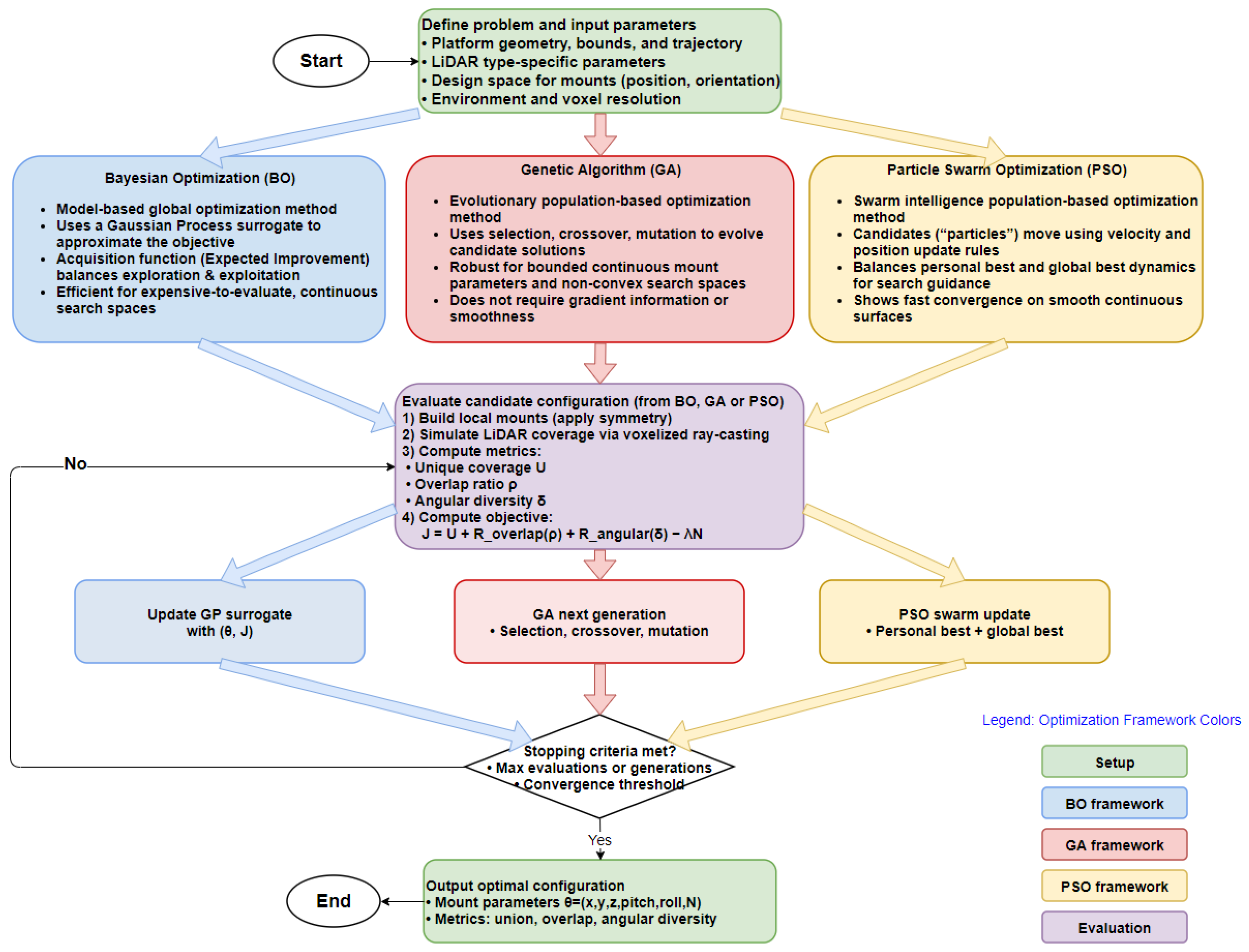
The proposed multi-LiDAR optimization framework consists of three components, as shown in the overall methodological workflow in
Figure 2. The first is LiDAR simulation using voxelized ray-casting, the second is assessment of coverage, overlap, and angular diversity, and the third involves iterative optimization with one of three strategies (Bayesian optimization, genetic algorithms, and particle swarm optimization) to find the optimal number of LiDAR units and their mounting parameters to achieve bilateral symmetry coverage. This is based on optimal master sensors, which are automatically mirrored across the platform’s centerline to establish a complete sensor array.
For any candidate configuration, the framework simulates LiDAR measurements along the platform trajectory and evaluates voxel-level visibility metrics, including unique coverage , overlap ratio (), and inter-sensor angular diversity . These metrics are combined into a scalar objective function , where denotes the vector of mounting parameters.
The optimization loop operates by repeatedly proposing candidate configurations (using BO, GA, or PSO), evaluating their performance through voxel simulation, and updating the optimizer until a global stopping criterion, such as a maximum number of evaluations or a convergence threshold, is met. The final output is the best-performing LiDAR configuration, along with all related coverage statistics and visualizations.
For clarity, the main geometric terms used in this study are defined. Coverage is the number of voxels or surface samples observed by at least one LiDAR. Overlap measures shared observations, as the proportion of voxels covered by at least two LiDARs. Redundancy is the repeated observation of the same area by multiple sensors. Observability refers to a configuration’s ability to observe relevant parts of the environment and minimize blind spots. Angular diversity is the separation between sensor viewing axes, promoting complementary rather than parallel sensing.
For each candidate configuration, the optimizer first identifies the active master sensors and then extends them to include the full set of physical sensors, in accordance with the symmetry rule. Each LiDAR moves along the platform’s trajectory, and at each position, a voxel-level ray-casting simulation is conducted based on the sensor’s beam geometry, vertical layout, azimuth sweep, and range. During this process, each beam assesses line-of-sight visibility within the voxel environment, ignoring occluded voxels. The visibility data from all sensors and positions are combined into a coverage map. From this map, the number of uniquely covered voxels, the proportion observed by at least two sensors, and the minimum inter-sensor angular separation are derived and fed into the objective function (
Section 3.2). This evaluation reflects the cumulative mapping performance over the entire path, rather than at a single point.
Mathematically, it is aimed to determine the optimal number of LiDARs and the mount parameters for each LiDAR, thereby maximizing overall environmental coverage subject to spatial and geometric constraints.
Each LiDAR mount
is defined by a position
and orientation vector
. The environment is modeled as a voxelized 3D volume
, and each voxel
vk can be visible or occluded based on the LiDAR line-of-sight simulation along the predefined mapping trajectory. Accordingly, the optimal sensor count
is defined as:
Mounting configuration for each sensor
i = 1, …,
where
represents the sensor position relative to the platform’s local reference frame.
∈ R3 represents the sensor orientation as the roll, pitch, and yaw angles.
The complete decision vector is:
where only the first
sensor configurations are active. The optimization variable
therefore belongs to a mixed discrete–continuous design space, where the sensor count
is integer-valued and the mount parameters
are continuous.
For each master sensor
i, the mirrored counterpart is defined in Equation (2). So, to ensure physically valid, left–right symmetric configurations while reducing the design search space by half, Equation (4) is introduced as:
where
is the mirrored counterpart of the sensor
generated by the symmetry operator
.
This symmetry operator directly incorporates reflectional invariance into the design space, thereby reducing the effective dimensionality of the optimization process while ensuring geometrically balanced sensor configurations. Symmetry about the centerline of the backpack or platform results in a compact and stable mobile mapping system. Mirroring lateral positions helps maintain payload balance and achieve comprehensive environmental coverage. If symmetry were aligned along the trajectory, it would prioritize front–back mirroring, which emphasizes the scan direction rather than lateral coverage. The pitch angle is represented in the lateral coordinate, with sensors configured outward in pairs. During the initial phase of searching for an optimal configuration, the roll angle is held at 0°. This is aimed at simplifying the search by reducing the number of dimensions in the optimization process and enabling realistic sensor mounting at 0° roll on a rigid platform. The main study thus investigates a limited yet meaningful set of laterally symmetric, zero-roll configurations, with other roll-related sensitivities examined separately in the robustness analysis.
The optimizer controls the mixed discrete–continuous variable (Equation (3)). For each candidate , the master mount is expanded using the symmetry operator (Equations (5) and (6)) to construct the full physical sensor set (Equation (7)), on which coverage, overlap, and angular-diversity rewards are evaluated to compute (Equation (8)).
3.2. Objective Function Formulation
The LiDAR mounting optimization is formulated as a discrete–continuous nonlinear optimization problem. The objective is to maximize scene coverage while regulating sensor redundancy, enforcing angular diversity, and penalizing excessive sensor count.
Denote the full set of physical LiDAR mounts, each parameterized by its position and orientation. For spinning 360° LiDARs (OS1-64 (Ouster, Inc., San Francisco, CA, USA) and VLP-16 (Velodyne Lidar, Inc., San Jose, CA, USA)), yaw has negligible influence on coverage due to full azimuthal sweep and is therefore excluded from the decision space.
The objective function is defined as:
where:
is the total number of uniquely covered voxels;
regulates coverage overlap;
promotes angular diversity;
is a per-sensor penalty coefficient;
is the total number of physical LiDAR sensors.
The objective function in Equation (8) is designed to reflect four key practical aspects of multi-LiDAR mobile mapping: optimizing scene coverage, preserving valuable inter-sensor redundancy, encouraging complementary viewing angles, and minimizing hardware complexity. The coverage term is predominant, as the primary goal of incorporating LiDAR sensors is to enhance the count of uniquely observed voxels. The overlap term acts as a regularizer that promotes sufficient shared visibility for cross-sensor consistency while preventing too much redundancy in observations. The angular-diversity component discourages sensors with nearly parallel axes and promotes a wider variety of viewing directions. At the same time, the sensor-count penalty stops the optimizer from adding sensors when the extra coverage is not justified by the hardware costs and complexity. The coefficients in the objective function are design-level parameters and not universal constants. They preserve the dominance of unique voxel coverage while allowing overlap and angular diversity to shape the configuration. Parameter λ was set to match the marginal coverage gain from adding another LiDAR, discouraging unnecessary sensors without hindering beneficial multi-sensor setups. The optimal values of the coefficients may vary by sensor type, environment, trajectory, and mapping goals because these coefficients reflect system priorities.
During optimization, the negative objective is minimized. Although the objective is expressed as a maximization problem in Equation (8), several optimization routines internally minimize the negative objective () for consistency. Throughout the results section, objective values are reported in their maximized (positive) form for clarity.
The coverage term represents the number of unique voxels observed by at least one LiDAR along the backpack trajectory:
Here, denotes the voxelized scene, and visibility is determined via a deterministic ray–box intersection simulation along the full trajectory.
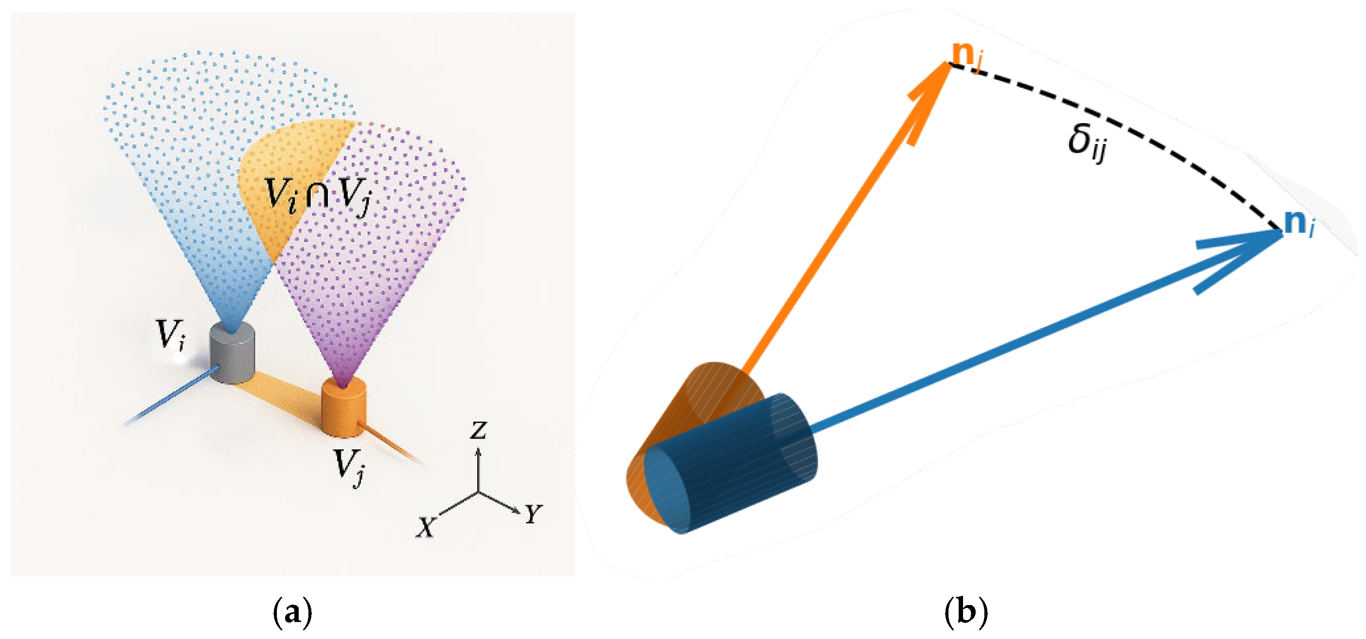
To maintain moderate multi-sensor redundancy, necessary for scan registration consistency, but avoiding excessive duplication, an overlap ratio is defined (
Figure 3a):
The overlap reward is defined as a piecewise linear function:
The overlap ratio
is calculated from the union of voxels along the simulated trajectory, reflecting multi-sensor redundancy across space and time rather than just an instantaneous overlap at a single pose. The range
serves as a soft-overlap regularization window in the objective function. This range encourages configurations with adequate shared visibility and discourages those with too little or too much redundancy. However, it remains balanced by the main coverage goal, the angular-diversity reward, and the sensor count penalty. As a result, the overlap percentages in
Section 4 are descriptive post-analysis metrics of the final optimized configurations and can surpass the regularization interval. Higher values indicate trajectory-aggregated shared coverage rather than strict interference violations.
This structure enforces:
- –
A penalty for insufficient overlap;
- –
A consistent reward within the preferred overlap window;
- –
A penalty for excessive redundancy.
Unlike weighted linear combinations, this window-based regulation explicitly focuses on functional overlap rather than maximizing redundancy.
To prevent nearly parallel sensor orientations and promote complementary viewing geometry, the minimum inter-sensor axis angle is defined as:
where
and
are unit vectors aligned with the local boresight (local +
Z axis) of LiDARs
and
(
Figure 3b).
The angular diversity reward is:
where
.
A wider angular separation between sensor viewing axes enhances the geometric conditioning of scan alignment and reduces degeneracy in planar environments.
This formulation:
The term improves geometric conditioning and reduces redundant directional sampling.
A linear penalty regulates system complexity: is applied per physical sensor. This term prevents trivial solutions with excessive LiDAR count and enforces a trade-off between coverage and hardware cost.
The proposed framework aims to be general and reproducible at the methodological level. However, the numerical coefficients in the scalar objective function serve as design parameters that vary based on the sensing scenario and system priorities. This variability is expected in multi-LiDAR optimization because LiDAR models vary in beam density, vertical angular coverage, range behavior, and redundancy requirements. Consequently, the coefficients should be viewed as physically motivated, transparent control parameters rather than arbitrary empirical constants. They are intended to consistently balance coverage uniqueness, functional overlap, angular diversity, and sensor-count penalties. Accordingly, the robustness and transferability of the framework depend on its structure and simulation pipeline, while the reliability of the parameterization is supported by cross-sensor experiments and the λ sensitivity analysis detailed later.
To reduce dimensionality and address practical mounting symmetry, only a subset of the “master” sensors is optimized. When symmetry is enabled, each master is mirrored deterministically across the vehicle YZ-plane: . The roll may be set at 0° (as noted in the experiments) to simplify mechanical mounting constraints. All objective components are assessed on the complete expanded sensor set (masters + mirrored counterparts).
A Minimum Center-To-Center distance is established to ensure adequate mechanical clearance between the two housings and provide a reliable means of preventing interference. The use of YZ symmetry will automatically correlate this spacing to one or more mirrored pairs of LiDARs. Therefore, this rule for determining mechanical clearance will serve as the basis for estimating the overall mechanical feasibility, rather than as an accurate collision model at the enclosure level. Additional methods to more accurately determine whether an interference exists could be developed and implemented in future research.
It is worth noting that for 360° spinning LiDARs like the OS1-64 and VLP16, the yaw mount angle has minimal impact on coverage since the azimuth sweep spans the full 0–360° range. Therefore, yaw is omitted from the decision space when testing spinning LiDARs. Additionally, a physical clearance is maintained between LiDAR housings by requiring a minimum center-to-center distance and under YZ symmetry for all LiDAR mounts. This prevents mechanical interference while only slightly reducing coverage and enhancing overlap behavior.
While angular-diversity terms support scan-registration stability, they are proxy indicators rather than direct measures of registration quality. As mentioned, the aim is to develop a computationally efficient optimization framework for multi-LiDAR mounting that involves both discrete and continuous variables. The objective focuses on geometric quantities evaluated through voxel-based simulations. In low-texture, planar, or repetitive environments, relying solely on angular diversity might not ensure accurate alignment. An extension could include a direct registration-quality measure, like scan-matching information-matrix conditioning, point-to-plane ICP covariance, surface-normal diversity, or degeneracy indices.
3.3. Bayesian Optimization Framework
This is a surrogate-based method for global optimization of expensive black-box functions [
16,
17]. It builds a probabilistic model of the objective function and iteratively chooses promising candidate solutions by maximizing an acquisition function that balances exploration and exploitation.
BO is especially well-suited to the multi-LiDAR configuration problem because each objective evaluation requires full trajectory-based voxel simulation, which is costly and precludes the use of analytical gradients.
The unknown objective is modeled using a Gaussian Process (
):
where
and
denote the mean and covariance functions, respectively.
At each iteration, BO selects new candidate configurations by maximizing an acquisition function, specifically the Expected Improvement (EI) criterion, balancing exploration and exploitation. The optimization proceeds as follows:
Sample the number of LiDARs and their mount parameters .
Simulate the resulting LiDAR coverage via vectorized ray-casting.
Evaluate the objective function and update the GP model with the new observation.
Continue until the maximum number of evaluations, is reached, or convergence is achieved.
This framework allows for efficient global search in situations where evaluations are costly. It gradually refines the surrogate model to find an optimal multi-LiDAR configuration that maximizes coverage while satisfying spatial and angular constraints. Each objective evaluation requires simulating sensors across trajectory poses, with approximately rays per pose. Accordingly, this results in a computational complexity of which motivates the use of surrogate-based optimization.
Algorithm 1 summarizes the Bayesian Optimization procedure implemented in MATLAB R2024b. It shows the sequence of surrogate model updates, acquisition function evaluations, and configuration expansions under bilateral symmetry.
| Algorithm 1. Bayesian Optimization Pseudocode for multi-LiDAR configuration design. |
| Input: |
| Platform bounds and trajectory |
LiDAR intrinsic parameters (vertical angles, range, FoV, divergence)
Environment voxel grid G |
| Optimization hyperparameters (, ρmin, ρmax, δmin), clearance d_min |
| Bayesian optimization settings (MaxEval = 300, acquisition, seeds, stallWindow = 50, relImpTol) |
| Symmetry + roll policy (YZ symmetry on/off; roll fixed value or free) |
| Output: |
| X* = {, | i = 1 … N_masters} (mirrored full set) Metrics: coverage U, overlap ρ, angular diversity δ, objective J |
| 1: Initialize Bayesian Optimization: |
| Surrogate ← Gaussian Process; Acquisition ← EI(+) Design variables: |
| Integer N_masters ∈ [1, Nmax] |
| For each master s: = (x, y, z, pitch, roll) Mirroring rule (YZ plane): θ′ = (−x, y, z, −pitch, roll) Roll policy: if fixed → overwrite roll = const each eval |
| 2: for k = 1 … MaxEval do//with stall-based early stop |
| 3: ← Acquisition(Surrogate) //masters only |
| 4: ← ExpandBySymmetry() //add mirrors |
| 5: if not ClearanceFeasible(, d_min) then //XConstraintFcn |
| 6: mark infeasible; continue |
| 7: end if |
| 8: for each sensor s in do |
| 9: ← θ_to_mount_local() |
| 10: ← simulate_bitmap(, , G, params, divergence = 0) |
| 11: end for |
12: ← OR_s(); counts ← ()
13: U ← Σ() |
| 14: ρ ← Σ(counts ≥ 2)/max(1, U) |
| 15: δ ← min_{i ≠ j} acos(z^_i · z^_j) //local +Z axes |
| 16: J ← U + R_overlap(ρ; ρmin,ρmax) + (δ; δmin) − ·|| |
| 17: Update Surrogate with (, J) //masters are BO vars |
| 18: if k ≥ stallWindow and relImprovement then break |
| 19: end for |
| 20: ← argmax_J over evaluated masters |
| 21: ← ExpandBySymmetry() |
| 22: Rebuild & score with realistic divergence for reporting |
| 23: Export: |
| JSON with mounts, symmetry, and trajectory |
| CSV with per-sensor contribution & unique voxels |
| Plots of geometry and coverage |
| Return θ*, U, ρ, δ, J |
The Bayesian Optimization budget was limited to 300 objective evaluations, including 12 initial seed points used to train the Gaussian Process surrogate. An adaptive stall-based early-stopping criterion was used to halt optimization when the relative improvement in the best objective value fell below a small tolerance over a fixed evaluation window. This approach helps ensure sufficient global exploration while preventing unnecessary evaluations once convergence occurs. In practice, convergence usually occurred well before the maximum evaluation limit was reached, confirming that the chosen budget serves as a conservative upper bound while keeping computational costs reasonable.
3.4. Genetic Algorithm (GA)
Genetic Algorithms (GA) are population-based evolutionary optimization techniques [
18,
19] that iteratively enhance candidate solutions using biologically inspired operators. GA is well-suited to the multi-LiDAR configuration problem because it can explore nonconvex, multimodal search spaces without gradient information.
Each chromosome directly encodes the decision vector
defined in Equation (3). The first element represents the integer-constrained number of master sensors
, while the remaining elements correspond to mount parameters. Only the first
blocks are active, and symmetry expansion generates the corresponding mirrored sensors as described in
Section 2.
The fitness of each chromosome is evaluated using the objective function defined in Equation (8). Coverage , overlap reward , and angular diversity reward are computed via full voxel-level simulation.
At generation , GA maintains a population of chromosomes . Three genetic operators are applied:
Selection (): probabilistic selection biased toward higher-fitness individuals.
Crossover (): recombination of chromosome segments between selected parents.
Mutation (): random perturbation of parameters to maintain diversity.
The population evolves according to:
Elitism ensures the best-performing chromosomes remain in the population.
Algorithm 2 summarizes the GA-based optimization procedure used to solve multi-LiDAR configurations.
| Algorithm 2. GA-based Dual-LiDAR Configuration Optimization |
| Input: bounds , objective J(x), symmetry rules, population size P, |
| crossover fraction pc, mutation rate pm, max generations T. |
| 1: Initialize population uniformly within |
| //First element integer-constrained: |
| 2: Evaluate fitness |
| 3: for to do |
| 4: ParentSet ← TournamentSelection() |
| 5: Offspring ← LaplaceCrossover(ParentSet) |
| 6: MutatedOffspring ← PowerMutation(Offspring) |
| 7: for each candidate do |
| 8: Expand master configuration by symmetry |
| 9: Evaluate via voxel simulation |
| 10: Compute fitness |
| 11: end for |
| 12: NewPopulation ← Elitism + MutatedOffspring |
| 13: NewPopulation |
| 14: end for |
| Output: |
The GA was set with a population size of and up to 100 generations. Tournament selection, Laplace crossover, and power mutation operators were used. Elitism was enabled to keep the top individuals across generations.
3.5. Particle Swarm Optimization (PSO)
Particle Swarm Optimization (PSO) is a population-based metaheuristic [
20,
21] in which particles continuously update their positions in the search space using both individual experience and shared information. PSO is ideal for the continuous parameter space of the dual-LiDAR configuration problem. Each particle represents the decision vector
defined in Equation (3). The first component encodes the integer-constrained number of master sensors
, while the remaining components correspond to mount parameters. During fitness evaluation,
is rounded to the nearest integer to enforce discrete sensor-count constraints. Symmetry expansion is applied before objective evaluation, as described in
Section 3.1.
The objective function evaluated for each particle is the global objective defined in Equation (8).
Particle velocities and positions are updated according to the standard PSO formulation:
is the inertia coefficient;
are cognitive and social acceleration constants;
are random scalars;
is the personal best solution found by the particle ;
is the global best position identified by the swarm.
The objective is identical to that of BO and GA and is evaluated after expanding master sensors by symmetry and performing voxel-level simulation.
PSO simultaneously balances exploration through inertia and exploitation through global-best attraction, making it especially effective for smooth yet nonlinear optimization landscapes, such as LiDAR coverage patterns.
Algorithm 3 summarizes the PSO-based optimization procedure for solving multi-LiDAR configurations.
| Algorithm 3. Particle Swarm Optimization for Multi-LiDAR Configuration Optimization |
| Input: bounds , objective , swarm size , parameters |
| 1: Initialize particle positions and velocities uniformly within |
| 2: For each particle : |
| Round the first dimension (number of masters) to the nearest integer |
| Compute fitness |
| Set personal best |
| 3: Set global best |
| 4: for to do |
| 5: for each particle do |
| 6: |
| 7: |
| 8: Round first dimension to nearest integer |
| 9: Compute fitness |
| 10: if then |
| 11: if then |
| 12: end for |
| 13: end for |
| 14: Apply hybrid local refinement (Pattern Search) to |
| Output: |
The swarm size was set to 60 particles with a maximum of 80 iterations. An inertia coefficient and acceleration constants were used. A hybrid pattern search refinement was applied to the best particle at termination to improve local convergence.
During optimization, higher sensor counts (Nmasters > 1) were occasionally explored by GA and PSO in early generations or iterations. However, due to the linear sensor penalty term ( = 2000) and decreasing marginal coverage gains, such configurations consistently yielded lower objective values and were naturally discarded by all optimizers. No instability was observed at discrete transitions, and rounding in PSO did not cause oscillatory behavior between adjacent integer values. This suggests that the mixed discrete–continuous formulation remains numerically stable across different search strategies.
4. Implementation and Experiments
4.1. Optimization Settings
This section outlines the implementation environment, optimization setup, and evaluation metrics used across all experiments. The following subsections specify the configurations for the VLP-16 and OS1-64 multi-LiDAR configurations [
9,
10].
The OS1-64 and VLP-16 LiDARs were selected because they represent two common but technically different classes of spinning 360° LiDAR sensors. The OS1-64 provides higher vertical channel density and denser vertical sampling. On the other hand, the VLP-16 LiDAR is a lower-channel, sparser LiDAR configuration widely used in mobile mapping and robotics studies. Evaluating both sensors allows the proposed framework to be tested under different sampling densities and vertical field-of-view conditions. This comparison is important because optimal mounting geometry is expected to depend on sensor-specific properties such as beam density, vertical angular distribution, and field of view.
All experiments were performed using MATLAB R2024b for the optimization frameworks (BO, GA, and PSO) and Blender 4.2 [
22] for 3D visualization. All simulations follow the same core optimization strategy (
Section 3.2 and
Section 3.3), which includes:
BO based on the expected-improvement-plus (EI+) acquisition function.
Coverage evaluation through voxelized ray casting within a bounded 3D environment.
A unified objective function that considers coverage, overlap regulation, angular diversity, and sensor count penalty.
Identical objective coefficients within sensor types unless otherwise specified.
A JSON file will be exported from the optimization algorithm run, storing each sensor’s configuration, LiDAR parameters, and trajectory poses, which the Blender tool then uses to visually reconstruct the optimized setup.
The experiments were simulated in a 50 × 50 × 20 m enclosed box with a floor and four vertical walls, which served as the test environment. The trajectory consists of 41 poses sampled every 1 m along a 40 m straight path to simulate a walking speed of approximately 1–1.5 m s
−1. This setup represents a backpack-mounted mapping system operated by a person. The backpack height is fixed at 1.60 m to ensure realistic ground clearance. Intrinsic LiDAR parameters were set according to the manufacturer’s technical documentation [
9,
10].
The 50 × 50 × 20 m voxelized indoor environment is selected as a controlled setup to isolate sensor-configuration effects and enable a fair comparison under identical conditions. To assess transferability, the optimized configurations were subsequently tested in a realistic scene with a high-resolution ground-truth mesh, following a loop-shaped trajectory, using a motion-distorted LiDAR simulation, and performing a surface-based completeness analysis. The experimental setup and optimization parameters are summarized in
Table 1.
The maximum number of master sensors is , which results in at most 10 physical sensors under bilateral symmetry.
Table 2 summarizes the reward coefficients used in the Bayesian Optimization process.
It is worth noting that all mounting parameters are provided in the local coordinate frame of the backpack or platform. The x-axis indicates the lateral left-right direction, the y-axis points forward-backward, and the z-axis measures vertical displacement relative to the backpack reference point, which is at a height of 1.60 m. During the optimization process, the platform moves along a straight 40-meter path within the voxelized environment. Symmetry is enforced across the YZ plane; thus, each master sensor is mirrored by flipping the x-coordinate and pitch, while keeping the y, z, and roll values unchanged. This approach ensures that positive and negative pitch angles correspond to symmetric LiDAR pairs mounted on opposite sides of the backpack, with the pairs tilted outward.
4.2. Results for OS1-64 System
4.2.1. Bayesian Optimization Results for OS1-64
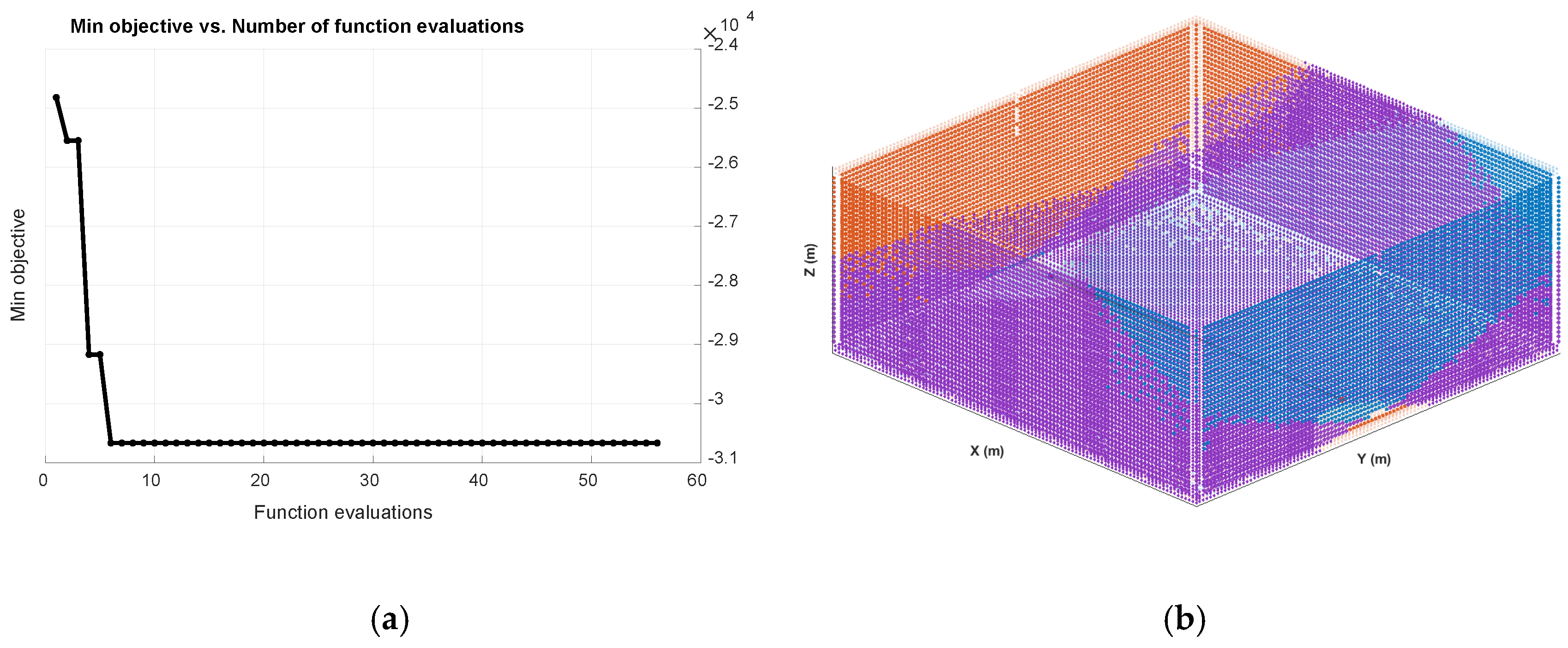
The system employed the BO algorithm with bilateral symmetry and a fixed-roll setup, similar to OS1-64. BO stopped after 56 function evaluations for the specified function, as it had not shown any relative improvement over the previous 50 evaluations, per the early-stopping rule incorporated into the experiment. The total BO duration was 25.41 seconds, with the objective function taking 7.47 seconds. The convergence curve of the minimum objective value is shown in
Figure 4, where a notable improvement of approximately 5851 between the two evaluation points (−24,817 to −30,668) is evident, followed by a plateau from the first six evaluations through the next 50. A good agreement is observed between the actual and predicted curves representing the objective function, indicating that the Gaussian Process surrogate model reliably captures the objective landscape.
The best feasible configuration corresponds to:
(expanded to two physical sensors under symmetry);
Objective value ;
Total unique voxel coverage ;
Overlap ratio ;
Minimum angular diversity .
Regarding individual contributions per sensor, each sensor typically observed 26,600 voxels, with an average of 8250 unique voxels across all sensors. The total overlapping area across all voxels is approximately 18,385, indicating a high level of redundancy among sensors in tracking angular diversity and providing sufficient overall coverage. The distribution of all 3D voxels is shown in
Figure 4b. Due to this symmetry during construction, coverage is expected to be concentrated along vertical surfaces, surrounding walls, and across the floor, while still offering ample angular diversity within the enclosed space. This coverage pattern demonstrates that a single symmetric controller configuration effectively serves this environment, as adding more master controllers did not improve the objective values. Overall, BO successfully identified a compact, symmetric configuration with high coverage and controlled overlap using fewer than 60 evaluations. The rapid convergence indicates that the surrogate model effectively guides the search within the mixed discrete–continuous design space.
4.2.2. Genetic Algorithm Results for OS1-64
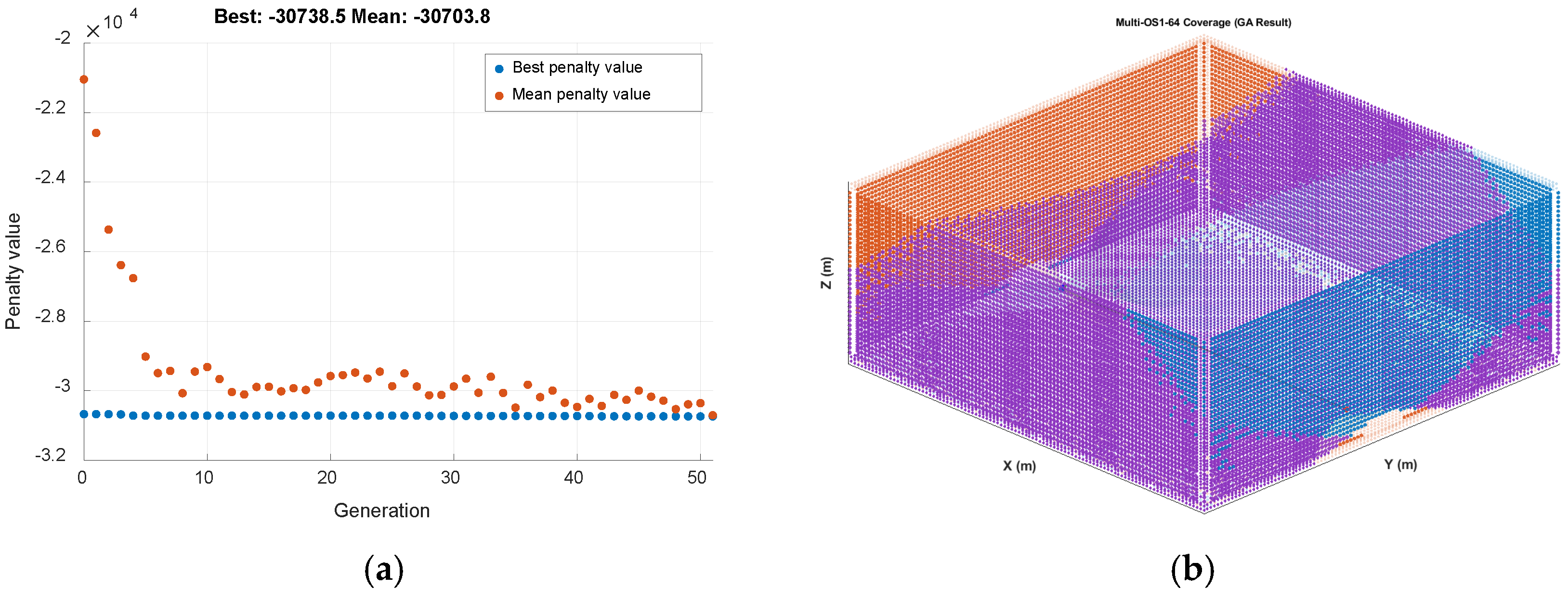
The Genetic Algorithm (GA) was applied to the OS1-64 configuration, maintaining the same symmetry and constraints as in BO. The problem involves 26 decision variables, including one integer variable (the number of master sensors). Tournament selection, Laplace crossover, and power mutation were all utilized. The optimization finished after 51 generations (3910 function evaluations) when the average change in penalty value dropped below the tolerance threshold. GA took much longer than BO due to its population-based approach, with a total time of 795.47 seconds. The results for the best and average penalties across generations are shown in
Figure 5a. The best objective is quickly approached, approximately −3.072 × 10
4 after the initial generations, the average population’s fitness gradually improved as convergence continued, and the population stabilized. After the 42nd generation, there may have been minor improvements, but no further enhancements occurred in subsequent generations.
The GA optimization converged on a symmetric dual-sensor configuration in which both OS1-64 units are mounted with a ±7.4 cm lateral offset, a 25 cm forward offset, and an 11.9 cm vertical offset relative to the backpack frame. The sensors are tilted outward with pitch angles of ±32.7°, creating a wide angular baseline (about 65.5°). This setup covers 34,906 unique voxels with roughly 56.9% overlap, demonstrating strong complementary wall coverage while maintaining redundancy.
The optimal configuration expands symmetrically into a dual-sensor configuration. Compared to BO, GA achieves slightly higher total coverage (+19 voxels) and a significantly larger minimum angular separation, but at the expense of increased overlap. The 3D voxel coverage density of the optimized arrangement is illustrated in
Figure 5b. The symmetry in the optimized arrangement also yields wall and floor densities similar to those in the BO; nevertheless, GA produces more diverse viewing directions on vertical surfaces than the BO does, due to its greater angular separation.
GA successfully identifies a high-quality configuration for the symmetric solution, with an objective function value similar to that of the BO. Nevertheless, using GA is computationally much more expensive than using BO (approximately 3910 evaluations compared to 56 for BO), thus demonstrating that surrogate-based optimization provides a clear efficiency advantage in solving this problem.
4.2.3. Particle Swarm Optimization Results for OS1-64
PSO was applied to the OS1-64 configuration with the same symmetry and constraint settings as in Bayesian Optimization and GA. The swarm size was determined using the parameters in
Section 3.5, and the optimization ran for 60 iterations until the stall criterion was met. A hybrid Pattern Search step was automatically activated after convergence, but did not further improve the solution. The total wall-clock time was 536.19 seconds, which is notably lower than GA but higher than BO, due to the population-based evaluation of particles each iteration.
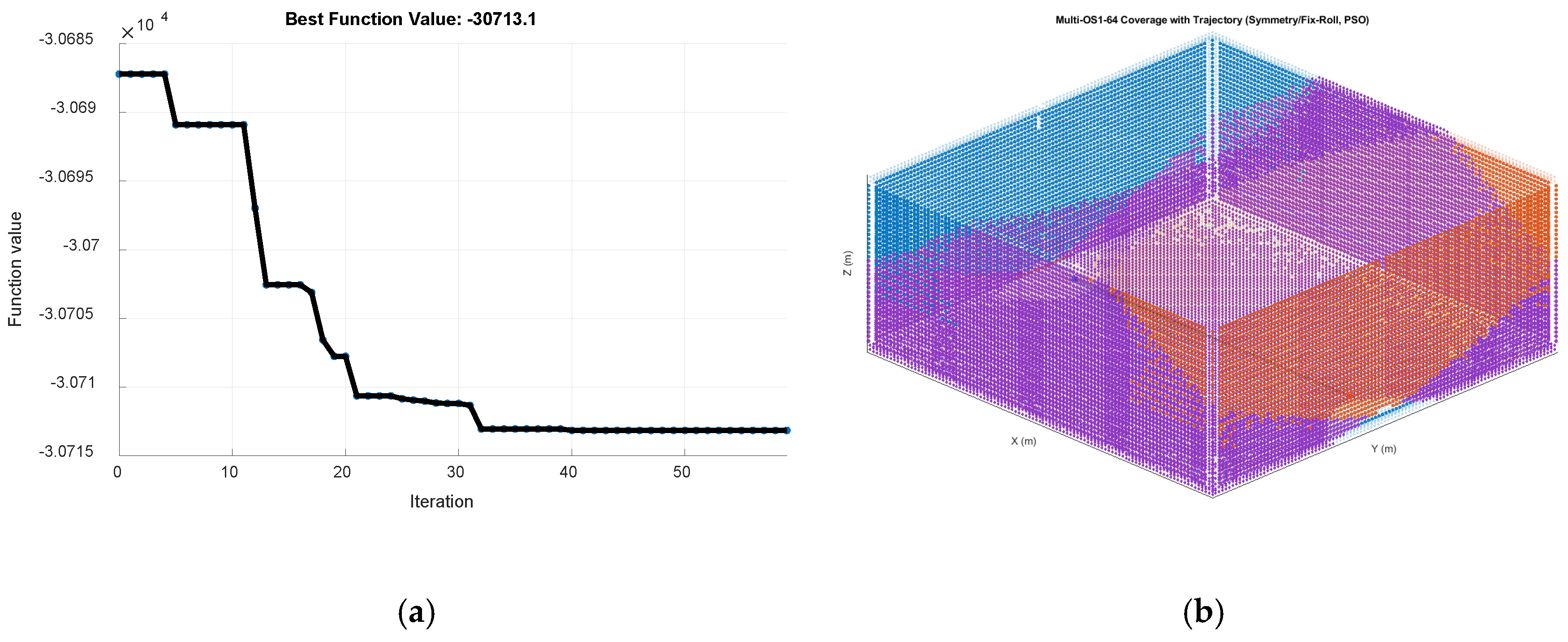
Figure 6a shows how the best objective value changes over iterations. The objective quickly drops within the first 20–30 iterations, reaching about
, then only slightly improves. The convergence curve appears smooth and steady, with no oscillations, indicating strong swarm dynamics and consistent progress in both the personal and global best solutions.
The PSO settled on a symmetric dual-sensor configuration in which both OS1-64 units are positioned at a lateral offset of ±2.8 cm, a forward offset of 17.0 cm, and a vertical offset of 2.0 cm relative to the backpack frame. The sensors are tilted outward with pitch angles of ±26.0°, creating a moderate angular baseline (about 52.0°). This setup covers 34,884 unique voxels with around 52.8% overlap.
The optimal controller configuration can be extended symmetrically to a dual-sensor configuration, similar to GA and BO solutions. Compared to GA, PSO achieves nearly the same total coverage (−22 voxels difference) and a slightly higher objective value, although with reduced minimum angular separation and somewhat lower overlap redundancy. The voxel distribution of the optimized setup is shown in three dimensions in
Figure 6b. Extensive wall and ground coverage across the environment can be achieved with symmetrical outward-tilted arrangements; however, the vertical walls exhibit less angular diversity, especially because the pitch magnitude is lower than in the GA results. PSO finds strong symmetrical solutions that are just as good as those from BO and GA in overall quality. Compared to GA, PSO is also significantly less expensive to run, requiring fewer evaluations (3420 versus 3910. The results from all three methods exhibit similar patterns across the three ground geometries, indicating the overall stability of the optimal setup throughout the entire search space.
4.3. Results for VLP16 System
4.3.1. Bayesian Optimization Results for VLP16
This paper used a Bayesian Optimization Framework for the VLP-16 configuration and employed the same symmetry and constraint setups (i.e., 12 Sobol Initiation Points and 68 Expected Improvement iterations) as in previous experiments. The optimization was constrained by bilateral symmetry about the YZ Plane and fixed roll at 0°. When performing optimization with 80 functions (all subject to this budget and others), the process involved 12 initial Sobol points followed by 68 Expected Improvement iterations.
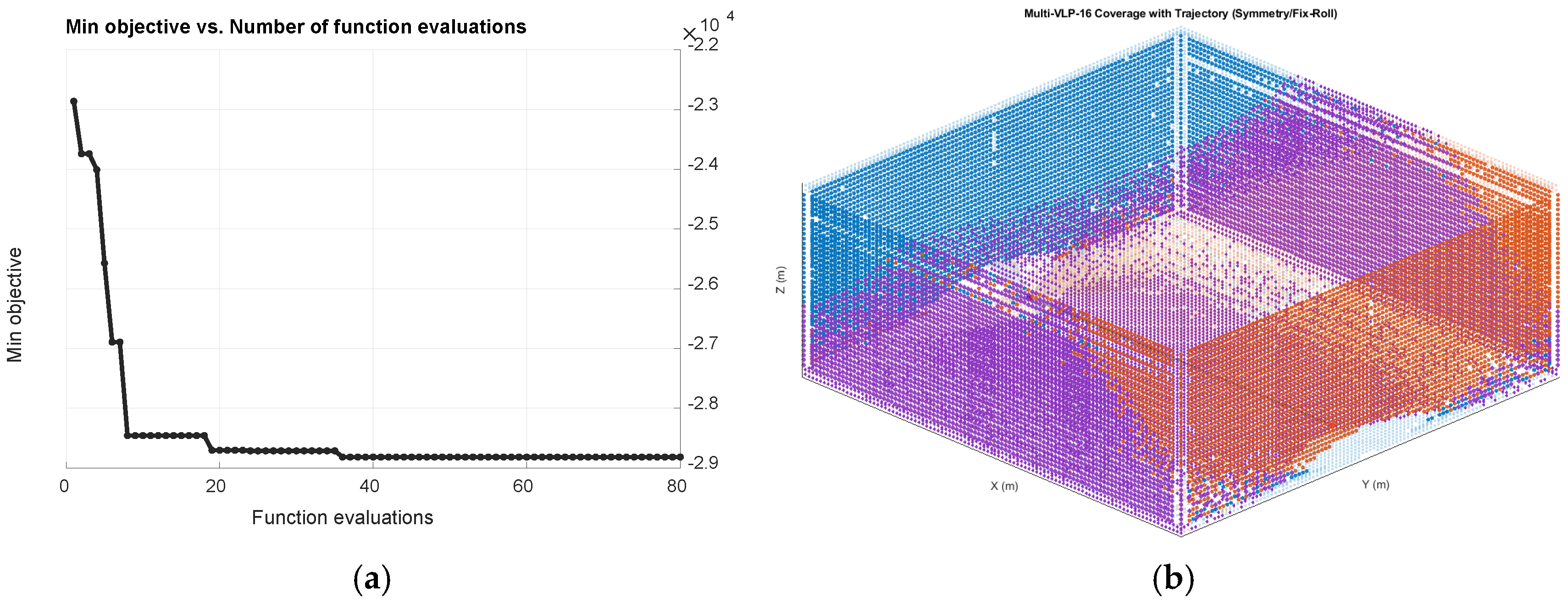
Figure 7a illustrates how the best objective value evolves during the optimization process. A quick decline in the objective occurs within the first 10–15 evaluations, indicating effective exploration of the search space. After about 30–35 evaluations, the improvement slows down, and the solution stabilizes, indicating that the Gaussian Process surrogate model has converged. The remaining evaluations show only minor improvements, confirming that the selected budget is adequate for this problem size. The BO converged to a symmetric dual-sensor configuration in which the two VLP-16 units are mounted with a ±3.65 cm lateral offset, a −11.84 cm forward offset, and a 11.53 cm vertical offset relative to the backpack frame. The sensors are tilted outward by ±25.23°, creating an angular separation of about 80°.
This configuration achieves approximately 33,000 uniquely covered voxels, with an overlap of 43–45%. The final objective value is J* ≈ 2.9 × 10⁴.
Figure 7b shows the three-dimensional voxel coverage of the optimized symmetric setup along the 40-meter path. This configuration provides balanced side wall coverage and maintains good ground visibility. The overlap exceeds the desired regularization window, consistent with the design, since the overlap serves as a soft regularization term rather than an absolute requirement. The comparatively large angular separation guarantees complementary viewing directions between the two sensors. The Bayesian optimization duration was less than one minute and involved only eighty objective evaluations. In comparison to population-based methodologies, this underscores the efficiency of surrogate-based optimization for computationally intensive voxel-level simulation problems.
4.3.2. Genetic Algorithm Results for VLP16
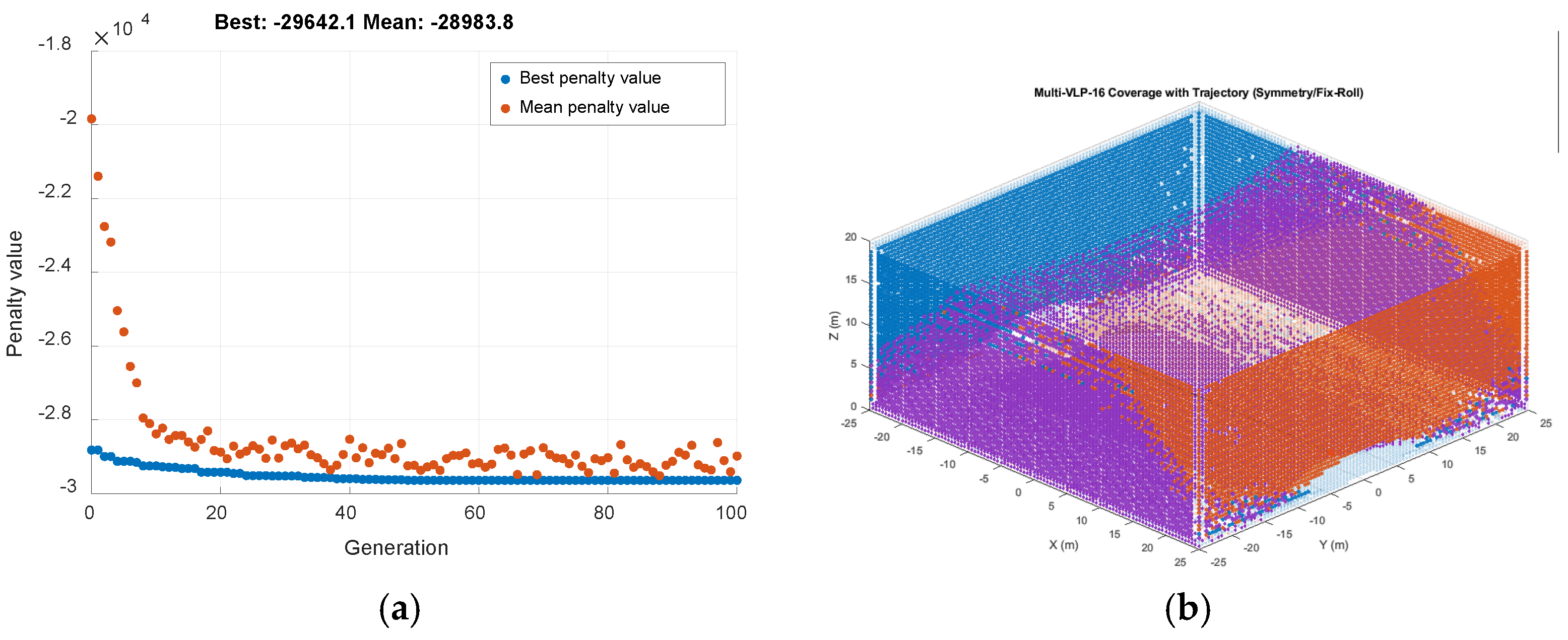
The Genetic Algorithm (GA) was applied to the VLP-16 configuration, using the same symmetry and constraint settings as in Bayesian Optimization. The problem included 26 decision variables, one of which is an integer variable that determines the number of master sensors. Tournament selection, Laplace crossover, and power mutation were used. The optimization ended after 100 generations (7585 function evaluations) when the average change in the penalty value dropped below the set tolerance. The total wall-clock time was 266.93 seconds.
Figure 8a shows how the best and average penalty values change over generations. The optimal objective value declines rapidly within the first 20–30 generations, reaching approximately −2.95 × 10
4, while the average fitness steadily increases and shows consistent convergence and population stabilization. After generation 40, only small gains are seen, and the solution levels off near the final objective value.
The GA optimization converged on a symmetric dual-sensor configuration in which both VLP-16 units are positioned at a lateral offset of ±7.0 cm, a forward offset of −0.4 cm, and a vertical offset of 11.8 cm relative to the backpack frame. The sensors are tilted outward at pitch angles of ±37.55°, resulting in an angular separation of approximately 75.1°. This setup covers 33,104 unique voxels with about 39.2% overlap, demonstrating effective complementary wall coverage with moderate redundancy.
The optimal controller setup expands symmetrically into a dual-sensor configuration.
Figure 8b displays the distribution of 3D voxel coverage for the optimized layout. Symmetric outward tilting ensures equal wall coverage in both directions along the corridor, while the relatively high pitch improves vertical surface visibility. VLP-16 coverage is slightly lower than OS1-64 due to its lower vertical channel density. Overall, GA successfully identified a stable, symmetric configuration for VLP-16 with a final objective value of 29,028.6. The overall solution quality is comparable; however, 7585 function evaluations show that population-based search techniques require much more computational resources than surrogate-based methods.
4.3.3. Particle Swarm Optimization Results for VLP16
Particle Swarm Optimization was applied to the VLP-16 configuration using the same symmetry and constraint settings as in Bayesian Optimization and GA. The swarm size was defined as in
Section 3.5, and the optimization proceeded for 56 iterations before the stall criterion was satisfied. A hybrid Pattern Search step was automatically triggered after convergence, but it did not yield further improvement. The total wall-clock time was 148.90 seconds, which is considerably lower than GA and moderately higher than BO, reflecting the population-based evaluation of particles at each iteration.
As shown in
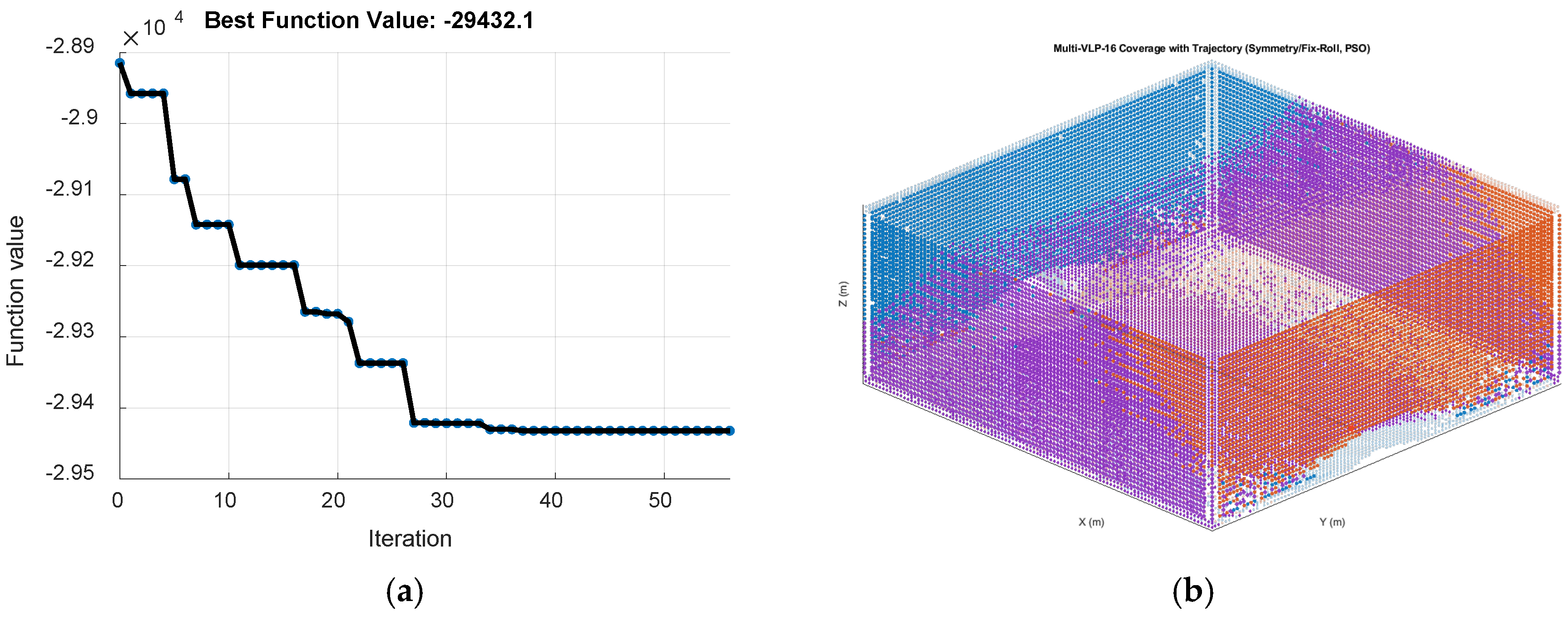
Figure 9a, the overall best value decreases rapidly during the first 25-30 iterations (to about 2.9 × 10
4), after which improvements become very small. The convergence curve is smooth and stable, showing no signs of oscillation, indicating a good balance between exploration and exploitation of the search space by all particles in the swarm, along with consistent communication of both personal and global best solutions. The PSO has successfully converged on a symmetric dual-sensor configuration using two VLP-16 sensors. Each sensor is positioned with a lateral offset of ±3.0 cm, a forward offset of −1.8 cm, and a vertical offset of 12.9 cm from the backpack frame.
The sensors are tilted outward with pitch angles of ±41.99°, forming a relatively wide angular baseline (≈84.0°). This configuration achieves 32,992 uniquely covered voxels with approximately 42.3% overlap.
The optimal controller configuration expands symmetrically into a dual-sensor configuration consistent with the GA and BO solutions. Compared to GA, PSO achieves slightly lower total coverage (−112 voxels) but a larger minimum angular separation, resulting in improved angular diversity and reduced overlap redundancy. Compared to BO, the coverage is similar but achieved with more pronounced pitch angles.
Figure 9b shows the 3D voxel coverage distribution of the optimized configuration. The symmetric outward tilt produces complementary coverage on vertical walls and on the floor along the trajectory. A larger pitch magnitude than BO results in greater angular separation, especially on vertical surfaces.
Overall, PSO effectively finds a high-quality symmetric configuration comparable to those of GA and BO for the VLP-16 system. While it is much faster than GA in terms of runtime and evaluations, it is still more computationally demanding than BO. The repeated appearance of symmetric dual-sensor geometries across all three methods further confirms the robustness of the optimal configuration in the VLP-16 search space.
4.4. Comparative Summary of Optimization Methods
This section reviews the quantitative performance of Bayesian Optimization, Genetic Algorithm, and Particle Swarm Optimization for both OS1-64 and VLP-16 dual-LiDAR configurations. All methods were run under the same environmental conditions, symmetry constraints, and objective formulations. A detailed comparison of objective values, coverage metrics, angular diversity, evaluation counts, and runtime is provided in
Table 3.
As illustrated in
Table 3, all three optimization methods attain similar final objective values and coverage metrics. Nonetheless, BO achieves this performance with significantly fewer objective evaluations compared to GA and PSO. This demonstrates that BO has a distinct efficiency advantage in evaluation under costly voxel-simulation conditions. Across both LiDAR models and all optimizers, the repeated recovery of bilaterally symmetric dual-sensor solutions indicates that symmetry is not merely imposed by design but is also reinforced by the objective landscape as a stable structural optimum. It should be noted that the overlap values in
Table 3 are descriptive post-analysis metrics that represent union voxels observed by at least two sensors. They are not limited to
. The overlap interval is a soft regularization window in the objective function. Higher values indicate shared coverage or redundancy, not violations of a hard interference constraint.
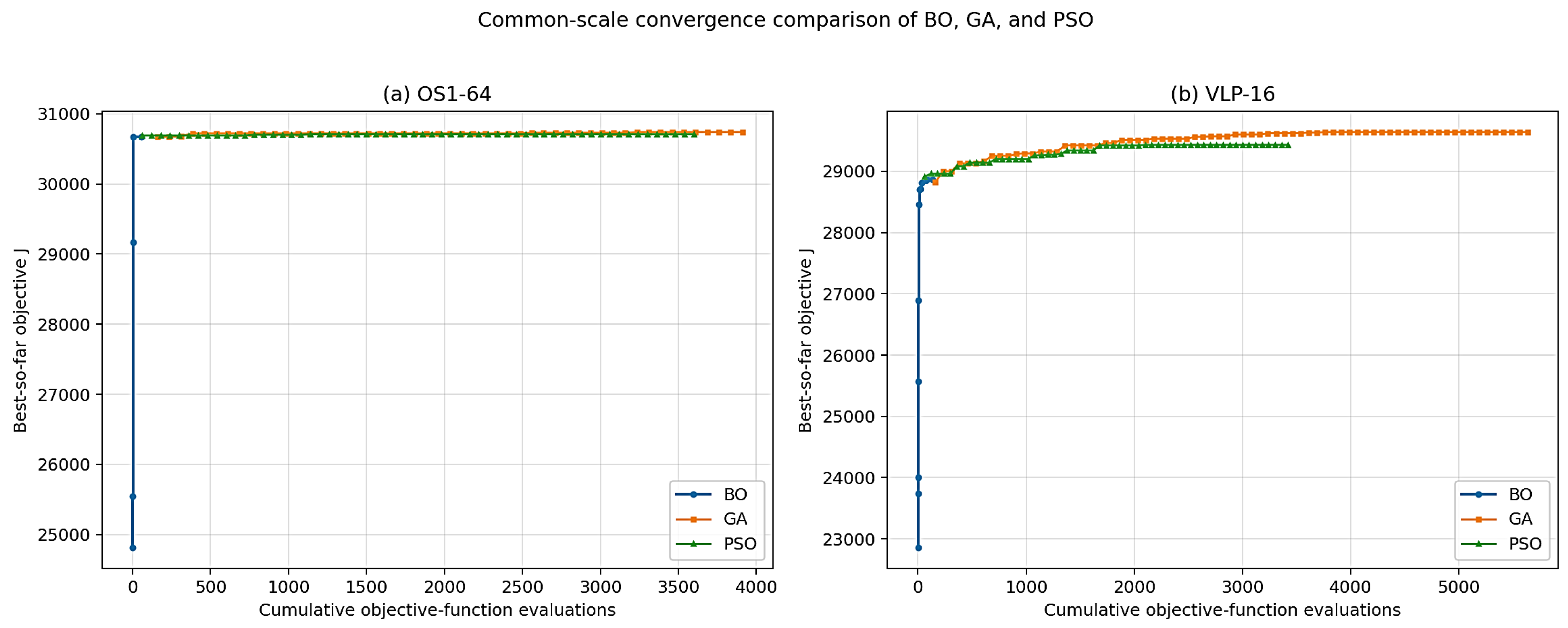
To compare computational efficiency, the convergence results of BO, GA, and PSO were replotted on a shared evaluation scale, as iteration counts differ: one BO iteration equals one evaluation, but a GA generation or PSO iteration involves multiple evaluations. Using cumulative evaluations provides a fairer comparison.
Figure 10 shows the best objective value,
, versus the cumulative number of evaluations for both LiDAR systems.
Figure 10 compares the convergence behaviors of BO, GA, and PSO on a shared evaluation scale. BO performs one evaluation per iteration, whereas GA and PSO perform multiple evaluations per generation or iteration, making cumulative evaluations a fair comparison. Results show that BO quickly reaches near-optimal values within a few evaluations for OS1-64 and VLP-16, whereas GA and PSO require thousands of iterations. This confirms BO’s efficiency in the voxel-simulation sensor-placement optimization problem.
It should be noted that was selected to approximately equal the average marginal coverage gain of a second sensor in preliminary experiments. A limited sensitivity analysis was performed by perturbing the sensor penalty coefficient by ±20% around the nominal value ( = 2000). For the OS1-64 configuration of the optimizer, the final result was an identical symmetric dual-sensor configuration across the tested values (lambda = 1600, 2000, 2400), with no change relative to the original pitch magnitude (25.23°), indicating complete invariance to moderate-scale changes in the reward. For the VLP-16 configuration, this same structure (symmetric dual-sensor) was optimal across all perturbations; however, there was moderate variation in pitch magnitude, with the maximum deviation at a lambda of 1600 (4.34°), and the overall sensor count and geometric domain structure remained unchanged. These results suggest that the structural optimum ( = 2 with bilateral symmetry) is resilient to moderate changes in penalty weighting, whereas fine angular tuning shows limited sensitivity in lower-channel sensors. This stability is consistent with the geometry of 360° spinning LiDARs, in which a second symmetrically mounted sensor already captures most of the remaining blind regions, so the marginal coverage gain from additional sensors decreases rapidly.
On the other hand, to compare computational efficiency independently of raw runtime or iteration count, two normalized efficiency indicators are introduced. The first indicator measures the objective gain per unit wall-clock time:
and the second measures objective gain per objective evaluation:
Higher values of these indicators reflect more efficient optimization in terms of computational cost relative to achieved objective quality. The resulting computational-efficiency metrics for the three optimizers and the two LiDAR systems are summarized in
Table 4.
For both LiDAR systems, all three optimization methods achieve similar objective values. For OS1-64, the total unique voxel coverage remains around 34,900 across all methods, whereas for VLP-16, it is approximately 33,000.
Differences among methods are most apparent in the overlap percentage and the minimum angular separation. For OS1-64, GA has the highest overlap (56.9%), while PSO shows the smallest angular separation (52.0°). For VLP-16, PSO has the largest minimum angular separation (84.0°), whereas GA has the lowest overlap (39.2%).
Regarding computational effort, GA and PSO require thousands of objective evaluations, whereas BO converges in fewer than 100 evaluations for both sensors. As a result, GA shows the longest total runtime in both sensor setups.
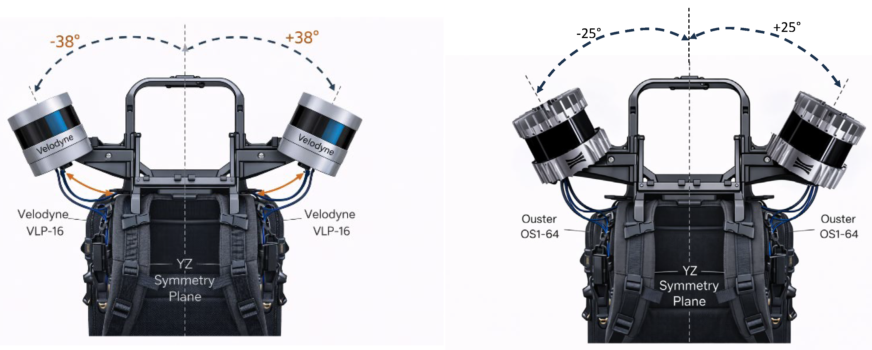
Figure 11 shows a photorealistic dual-LiDAR configuration derived via Bayesian Optimization for the Velodyne VLP-16 (left, ±38°) and the Ouster OS1-64 (right, ±25°). Both configurations preserve YZ-plane symmetry. The larger outward tilt of the VLP-16 compensates for its narrower vertical field of view, while the OS1-64 requires less angular divergence because of its higher channel density and wider vertical coverage.
4.5. Post Optimization Validation
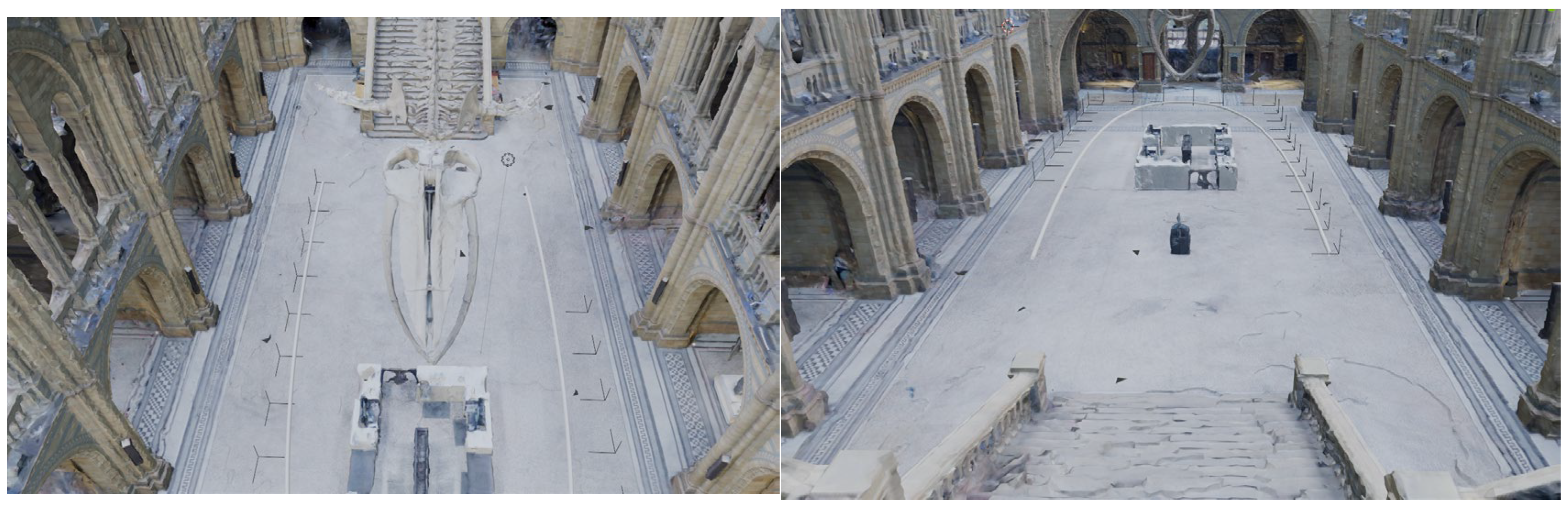
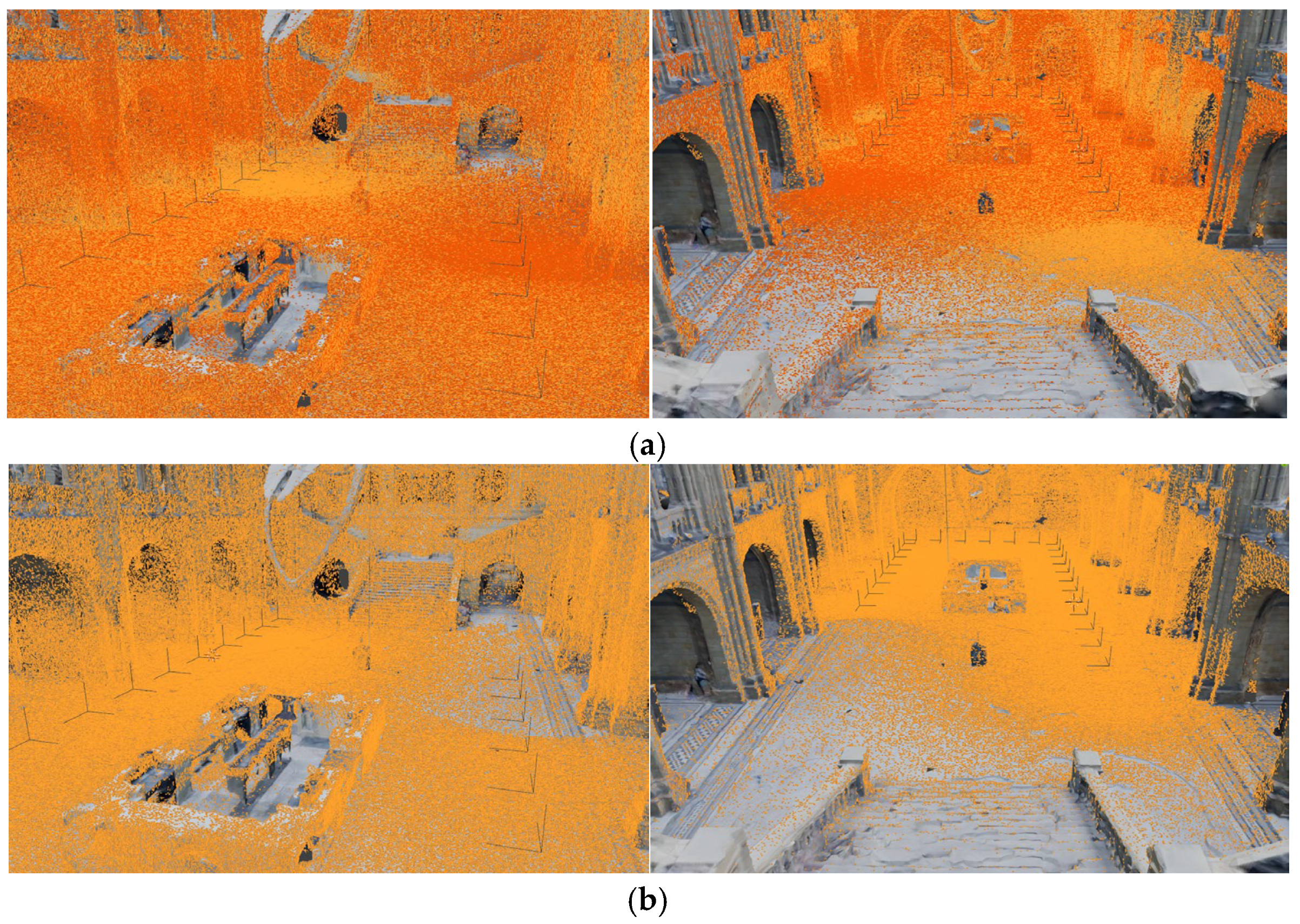
Unlike the voxel-level objective used during optimization, post-optimization validation evaluates surface-based geometric completeness against a high-resolution ground-truth mesh of an indoor environment shown in
Figure 12. The ground-truth model in this validation is a measured mesh and serves as the reference geometry for evaluating the simulated LiDAR point clouds. To analyze surface completeness, the mesh was sampled uniformly to generate 10 million reference surface points. A ground-truth point was considered covered if its nearest simulated LiDAR point was within a specified distance threshold of 0.05 meters. The same sampling method, distance threshold, trajectory, and comparison approach were applied for all single- and dual-sensor setups to ensure consistent comparison between OS1-64 and VLP-16 results.
Although this stage employs realistic trajectories, motion distortion, and surface-based comparison with a high-resolution ground-truth model, it remains simulation-based and does not fully account for real-world effects such as measurement noise, calibration drift, user-body occlusion, synchronization errors, or mounting tolerances.
4.5.1. OS1-64
To assess the practical effectiveness of the optimized dual-LiDAR configurations, a physics-based simulation was performed in Blender. The optimal mounting parameters from BO, GA, and PSO were applied to a realistic backpack-mounted dual Ouster OS1-64 system. The system was simulated walking along a closed-loop polyline trajectory at 1.2 m/s, with the LiDAR spinning at 10 Hz. Motion distortion was enabled to simulate real-world data-collection conditions. The resulting point clouds were exported and compared to a high-resolution ground-truth (GT) mesh using surface-based coverage analysis in CloudCompare [
23]. Surface coverage was calculated by uniformly sampling the GT mesh and measuring the percentage of surface samples within a fixed distance threshold from the simulated point cloud.
As a baseline reference, only one OS1-64 sensor (BO configuration) was activated. From the GT-sampled point cloud of 10 million points, the mapping system with a single OS1 covered 3,684,605 points. This shows that a single OS1-64 sensor mounted on a backpack captures about 37% of the scene during a single walking loop. The missing coverage is mainly due to occlusions, a limited vertical field of view (42.4°), and geometric shadowing.
All three optimization strategies were evaluated under identical simulation and threshold conditions (
Table 5).
Using GA as the best-performing method: = 47.97-36.85 = 10.03″% points.
This corresponds to:
+1,112,432 additional GT surface samples;
~27% relative improvement over single-sensor baseline.
This confirms that:
The second LiDAR significantly improves scene observability.
Symmetric angular placement provides complementary visibility.
The optimization algorithms refine performance within a ~1.5% range.
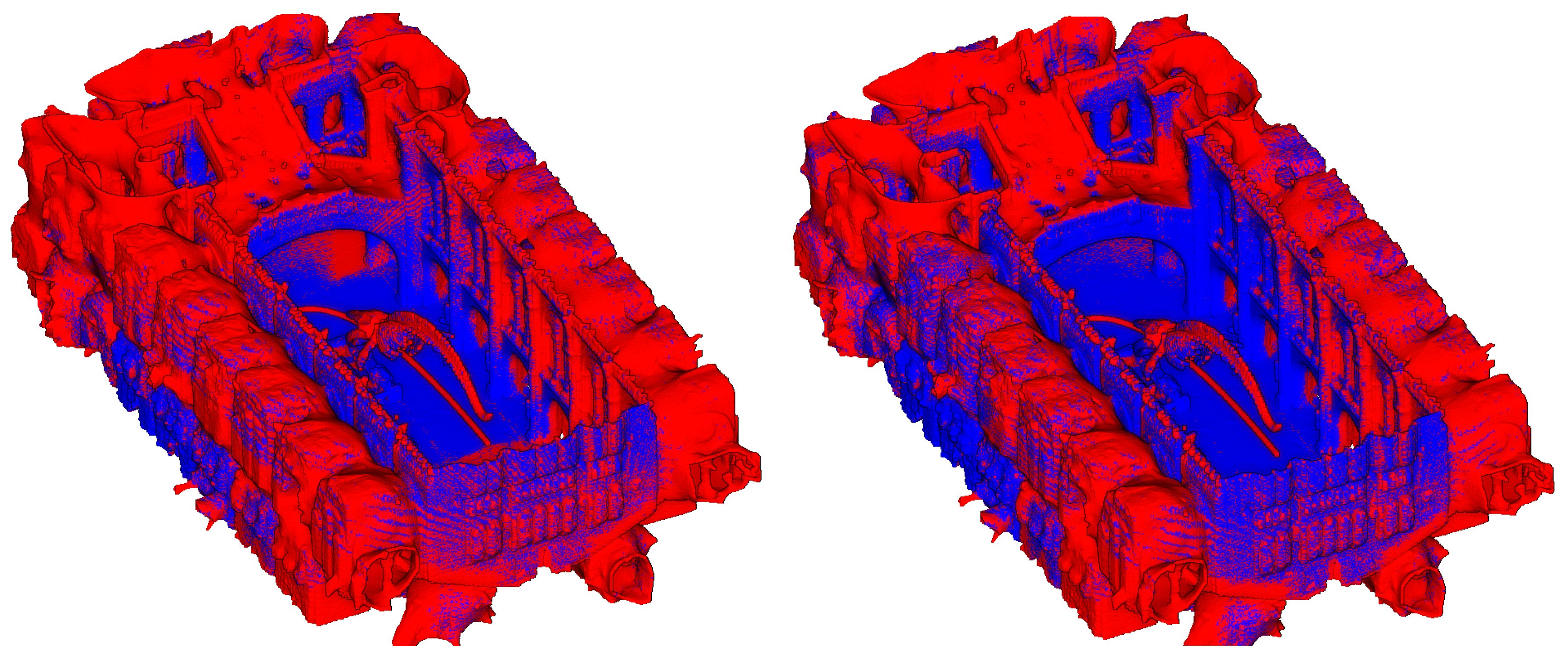
The point-cloud comparison between the single- and dual-sensor configurations is shown in
Figure 13.
4.5.2. VLP-16
To evaluate the effectiveness of the optimized dual-LiDAR configurations for the VLP-16, the best mount parameters obtained from BO, PSO, and GA were exported and simulated in Blender using a realistic walking trajectory. The LiDAR model incorporated:
16 vertical beams;
30° vertical field of view (−15° to +15°);
180 azimuth samples per revolution;
10 Hz spin frequency;
1.2 m/s walking speed;
Motion distortion enabled.
Coverage was computed by comparing the generated point clouds against the ground-truth (GT) mesh using surface sampling in CloudCompare.
Single-Sensor Baseline
A single VLP-16 mounted on the optimized configuration produced:
This establishes the geometric limitation of a single 16-beam sensor in the tested environment.
All three optimization strategies were evaluated under identical simulation and threshold conditions (
Table 6).
All optimization methods achieved similar performance, with GA yielding the highest coverage of 37.41%. The differences between methods remained below 0.7 percentage points, indicating that sensor geometry plays a larger role than the optimization strategy.
Relative to the single-sensor baseline: 37.41 − 26.41 = 11.00% points. This corresponds to a 41.7% relative improvement in surface coverage.
The visual comparison supports the quantitative improvements shown in
Table 5. The dual LiDAR configuration greatly improves coverage of vertical walls and interior structural elements, which are only partially captured by the single-sensor setup. Areas still not covered are mostly in deep concave shapes and under structural overhangs, which belong to physical occlusion rather than unfavorable mounting angles. This found configuration confirms that a symmetric outward-pitch design effectively enhances multi-view visibility.
Figure 14 shows the surface-completeness comparison for the optimized dual VLP-16 configuration.
In absolute terms, the dual configuration covered approximately 1.1 million additional GT samples compared to a single VLP-16. The absolute and relative improvements in surface coverage for both LiDAR systems are summarized in
Table 7.
The post-optimization validation confirms that the proposed optimization yields measurable gains in real-surface completeness.
5. Discussion
The experimental results show that the proposed mixed discrete–continuous optimization framework reliably finds symmetric dual-LiDAR configurations that balance coverage, overlap control, angular diversity, and hardware cost. Although Bayesian Optimization, Genetic Algorithm, and Particle Swarm Optimization use very different search strategies, all three methods tend to find physically feasible, bilaterally symmetric two-sensor configurations for both OS1-64 and VLP-16 systems. This convergence toward similar geometric arrangements offers valuable insights into the structure of the underlying optimization landscape. From a robotic perception perspective, increasing angular separation and implementing controlled redundancy are likely to enhance the geometric conditioning of multi-view registration. However, since a comprehensive SLAM evaluation was not performed, this study does not claim to improve pose-estimation accuracy or loop-closure robustness.
5.1. Stability of the Optimal Configuration Structure
In response to RQ1, all three optimization methods (BO, GA, and PSO) consistently converged to symmetric dual-sensor configurations under the same mixed discrete–continuous formulation. Despite variations in search methods and evaluation budgets, the resulting mount geometries show similar outward pitch directions and coverage statistics. This consistency among the three methods suggests that the best structural solution is robust to different optimization strategies and not restricted to any one of them.
A notable result is that all optimizers consistently selected a single master sensor, which was then, by symmetry, expanded into two physical LiDAR units. Higher-sensor-count configurations were considered during optimization but were not retained in the final optimal solutions. This indicates that adding more LiDARs does not provide sufficient additional coverage to justify the increased hardware cost. Additionally, the results reveal that increasing coverage, overlap, and angular diversity is redundant once two LiDARs are configured. Once sufficient wall and floor coverage and angular diversity are achieved, additional sensors primarily add overlap redundancy rather than new voxel views. Therefore, the regularization term helps avoid over-parameterization and encourages compact, mechanically feasible configurations. The similar results from BO, GA, and PSO illustrate that the symmetric two-sensor setup is a stable optimal solution rather than an artifact of any specific optimizer. This indicates that bilateral symmetry is a key structural feature of the optimal solutions under the tested objective.
Although the main optimization was performed in a simplified enclosed setting for controlled testing, the persistent emergence of outward-tilting symmetric configurations suggests that the solution is influenced by fundamental visibility trade-offs rather than only by the exact placement of walls. Early experiments in a more complex indoor environment (
Section 4.5) confirm that the optimized setups continue to perform well with loop-shaped trajectories and realistic 3D geometry.
Worth noting that the straight trajectory used during optimization was intended to isolate the effect of sensor configuration and ensure fair comparison among optimization methods. The loop-trajectory validation in
Section 4.5 provides initial evidence of the effectiveness of the linear trajectory setup. The broader trajectory sensitivity is a matter of future work.
5.2. Coverage–Overlap–Angular Diversity Trade-Off
Regarding RQ2, the results show a clear trade-off between maximizing unique coverage, controlling overlap within a certain range, and improving inter-sensor angular diversity. The total unique voxel coverage is similar among optimizers for each sensor type. However, variations are more shown in overlap percentages and minimum angular separation.
For OS1-64:
- –
GA yields the highest angular separation.
- –
BO and PSO produce slightly lower separation but comparable coverage.
- –
GA also results in increased overlap.
For VLP-16:
- –
PSO produces the largest angular separation.
- –
GA achieves slightly higher unique coverage.
- –
BO balances angular separation and overlap most conservatively.
These differences illustrate distinct optimizer behaviors as follows:
- –
The GA method explores wider angular ranges and occasionally results in larger pitch angles. This is improving angular diversity but may also lead to redundancy.
- –
The PSO method rapidly converges to smooth and continuous regions. It often identifies angular baselines when the conditions favor gradient-based search behaviors.
- –
The BO method, when guided by a surrogate model, usually enhances small areas with high objective values. It commonly produces balanced solutions that show moderate angular diversity and manage overlap effectively.
Notably, objective values are quite consistent through these optimization methods. This shows that several nearby configurations generate similar results and imply a relatively flat optimum region in the design space rather than a sharp, isolated peak.
5.3. Sensor-Specific Behavior: OS1-64 vs. VLP-16
The total area covered by the OS1-64 multi-LiDAR system consistently exceeds that of the VLP-16 sensor across all three optimizers. This is to be expected when using the OS1-64, as it has greater vertical channel density and higher vertical sampling resolution than the VLP-16. However, the relative differences between the optimization techniques are maintained with both sensors. The VLP-16 optimal system should have a larger pitch angle than the OS1-64 because it requires a greater vertical angular distance between sensors to compensate for the small number of vertical channels. The optimization framework automatically adjusts the mount geometry based on each LiDAR’s characteristics and adapts configurations within hardware limitations. This flexibility confirms that the proposed framework not only optimizes spatial placement but also optimizes geometry. However, the trajectory geometry can still affect the exact optimal mounting parameters, especially the preferred pitch, overlap structure, and the marginal gains from additional sensors.
In this study, a straight trajectory was deliberately used during the optimization phase to isolate the geometric impact of sensor placement, facilitate a fair comparison among BO, GA, and PSO, and keep repeated full-trajectory voxel simulations computationally feasible. The subsequent validation in a more realistic indoor scene, using a high-resolution ground-truth mesh and loop-shaped trajectory, provides initial evidence that the recovered symmetric dual-sensor arrangement is not merely a byproduct of the simplified box environment. Nevertheless, directly optimizing in cluttered, multi-room, outdoor, or strongly nonlinear trajectory settings may affect detailed mounting parameters, such as pitch, overlap structure, and the marginal benefit of additional sensors. Therefore, systematic sensitivity analysis across more complex environments and trajectories remains an important direction for future work.
An important insight arises from the post-optimization surface-based validation. Although OS1-64 consistently achieves higher absolute voxel coverage due to its denser vertical sampling, the proportional improvement in surface coverage from adding a second sensor is greater for the VLP-16 system. While both sensors show roughly a 10–11 percentage-point absolute gain in surface completeness, the relative improvement is about 42% for VLP-16 compared to around 27% for OS1-64. This indicates that lower-channel LiDARs benefit more, proportionally, from symmetric multi-sensor configurations. In other words, a multi-LiDAR configuration more effectively compensates for sparse vertical sampling than does an already dense beam arrangement. These observations confirm that different optimizer behaviors explore the same underlying trade-off surface rather than fundamentally different geometric solutions.
The results for VLP-16 also show a small difference between the GA and PSO solutions. GA produced the lowest post-analysis overlap, whereas PSO produced the largest minimum angular separation. This difference is expected because the two algorithms explore the design space differently. GA keeps several competing layouts active through crossover and mutation, which can help it avoid unnecessary shared coverage. PSO, on the other hand, gradually pulls the particles toward the best-performing region found by the swarm, and in this case, that region favored a wider angular baseline between the mirrored sensors. Therefore, the differences between GA and PSO are mainly reflected in the balance between overlap and angular diversity. They do not change the main geometric conclusion, since both methods still recover the same general configuration: a symmetric, outward-tilted dual-LiDAR arrangement.
5.4. Computational Efficiency and Practical Implications
The primary distinction between the optimization methods lies in computational efficiency. BO typically requires fewer than 100 evaluations for both sensor cases, whereas GA and PSO require thousands of evaluations. The difference is significant since each evaluation entails a complete trajectory-based voxel simulation. Surrogate-based modeling enables the BO method to model the objective requirement, balance exploration and exploitation effectively, and avoid unnecessary evaluations in regions of poor performance. Conversely, the GA method focuses on maintaining global diversity, which increases evaluation costs. The PSO method shows smoother convergence but still requires evaluating large swarms at each iteration.
From a practical system design perspective, the evaluation cost is expected to increase as LiDAR is simulated in more complex environments, such as adding dynamic obstacles or higher voxel resolution. In such scenarios, surrogate-based optimization is more advantageous, making BO the most computationally efficient method for expensive mixed discrete–continuous LiDAR configuration problems. Validation after optimization supports this finding since each configuration was re-simulated with realistic spinning behavior, motion distortion, and ground-truth surface comparisons, which requires more computation than voxel-level evaluation alone. Under these high-fidelity validation conditions, the difference in computational effort between fewer than 100 evaluations with BO and several thousand evaluations with GA or PSO is practically significant. When multi-LiDAR configuration optimization is part of larger system design processes or repeated across multiple environments, surrogate-based strategies provide notable scalability benefits. Worth mentioning that the computational complexity per evaluation is , which explains the high evaluation cost and motivates the use of surrogate modeling.
5.5. Effect of Symmetry Constraints
The proposed method imposes bilateral symmetry, which considerably reduces the search space while ensuring mechanical feasibility and balance for a mobile mapping backpack system. In all experiments in
Section 4, the optimizers consistently maintained symmetric configurations, even when exploring asymmetric intermediate solutions. Thus, symmetry is not only a practical constraint but also a structural asset. Symmetric outward pitch angles generate complementary viewing directions that improve lateral wall visibility and ensure registration overlap. This observation aligns with the design principles of commercial multi-LiDAR platforms and indicates that symmetry constraints are a logical design simplification rather than a limiting assumption.
The present study does not include a direct comparison with fully unconstrained optimization. Instead, it focuses on symmetry as a practical geometric prior for multi-LiDAR system design, rather than treating it as an auxiliary restriction. The results show the effectiveness of symmetry-constrained optimization in the tested context. However, a formal comparison between constrained and unconstrained optimization remains an important direction for future work.
5.6. Robustness of the Mixed Discrete–Continuous Formulation
This research problem combines discrete LiDAR-count and continuous mount positioning with the formulation of nonlinear visibility and piecewise reward structures. All three optimizers converge reliably despite this complexity. This shows that the mixed discrete–continuous design remains manageable with physically grounded evaluation metrics. The piecewise overlap reward and angular-threshold setup provide stable gradients for optimization, preventing issues such as excessive overlap or overly trivial parallel orientations. The alignment between voxel coverage in simulation and mesh-level completeness suggests that the overlap window, angular diversity reward, and sensor penalty collectively reflect actual mapping quality rather than merely theoretical geometric metrics.
From a robotics systems perspective, increased angular diversity and intentional redundancy are enhancing the stability of downstream registration and scan-matching tasks. However, these effects are only inferred in this study, as they were not directly tested within a SLAM pipeline. Consequently, this work primarily demonstrates improved geometric completeness and more systematically organized multi-view baselines. It does not provide direct evidence of enhanced SLAM consistency or pose-estimation accuracy. The computed LiDAR configurations remain relevant for subsequent mapping processes because they reduce blind spots, support cross-view consistency, and ensure more complementary viewing angles. While these qualities are significant for registration and SLAM applications, they are regarded here as geometric proxy benefits rather than confirmed outcomes of SLAM.
Regarding RQ3,
Section 4.5 shows that configurations optimized in a simplified voxel-based setting retain their geometric effectiveness on realistic surface-based ground-truth models. The consistent 11% increase in surface completeness demonstrates that the voxel-level goal effectively captures physically meaningful coverage, rather than merely fitting the optimization environment.
Robustness of the solution also depends on calibration and assembly uncertainties. The current optimization assumes exact mount parameters, but real-world errors can shift sensor positions by centimeters or degrees. Such errors may affect overlap, angular diversity, and visibility. Therefore, a sensitivity analysis of positional and assembly tolerance errors, for example, with ±1–2 cm and ±1–2° perturbations, would further assess robustness under actual hardware conditions. Although BO, GA, and PSO converge on similar configurations, analyzing their sensitivity to calibration errors is a valuable future step.
In addition, a brief roll-sensitivity analysis was performed using the BO framework for both VLP-16 and OS1-64 sensors at fixed roll angles of 0°, ±5°, and ±10°, as well as in a free-roll scenario (
Table 8).
The optimizers always converged to the same solution, a symmetric dual-sensor configuration (n = 2) across all conditions tested. The variations in the roll angle had only a small effect, primarily resulting in slight changes in angle and voxel coverage. For OS1-64, the fixed roll angles of ±5° and ±10° were close to the zero-roll baseline, whereas the free-roll condition yielded a lower objective value and reduced coverage. For VLP-16, the results suggest that the zero-roll assumption used in the main experiments is reasonable. The variations in the roll did not significantly affect the range tested for the main structural optimum.
The validation in
Section 4.5 shows geometric transferability in a high-fidelity simulation but should not be considered a final hardware verification. However, real-world experiments are still needed to evaluate the expected benefits in the presence of noise, occlusions, and small assembly errors. Such tests should use a physical backpack with dual-LiDAR mounting, calibration, and repeatable walking routes.
6. Conclusions
This work proposes a complete optimization framework that uses mixed discrete-continuous methods to design symmetric multi-LiDAR systems for mobile mapping platforms. The proposed approach combines physical simulation with Bayesian Optimization, Genetic Algorithm, and Particle Swarm Optimization to automatically find configurations that maximize coverage, minimize overlap, maximize angular diversity, and minimize the number of sensors. The results show structural stability, measurable geometric trade-offs, and successful implementation on real-world mapping, answering the three research questions posed in
Section 1. All three optimization methods converged to symmetric dual-sensor configurations, consistently for both the OS1-64 and VLP-16 LiDAR systems. Results showed that two well-aligned symmetric LiDAR units can achieve near-optimal coverage in the tested indoor environment. The study addresses a practical need in mobile mapping system design. It also shows that bilateral symmetry is a robust design principle for multi-LiDAR configurations, since symmetric dual-sensor configurations were consistently obtained across different optimizers, sensor types, and moderate parameter changes. Bayesian Optimization was the fastest of the tested approaches, requiring fewer than 100 objective function evaluations, whereas GA and PSO required thousands of evaluations, each of which was a complete trajectory-based voxel simulation. Therefore, surrogate-guided optimization offers a practical advantage for resource-intensive sensor placement tasks.
Post-optimization validation, including realistic trajectory simulation and surface comparison to a high-resolution ground-truth mesh, strongly supports practical transferability under high-fidelity simulation conditions. Nevertheless, because the entire process is still simulation-based, real-world hardware testing with actual sensors is required to confirm full validation.
Using a symmetric dual-LiDAR setup, compared to a single-LiDAR setup, improved surface completeness by roughly 11% scanned points. This resulted in relative improvements of ~27% and ~42% for OS1-64 and VLP-16, respectively. The agreement between voxel-level optimization and mesh-level validation suggests that the proposed objective captures meaningful physical coverage. It is therefore not limited to abstract geometric quantities. As shown in
Section 4.2 and
Section 4.3, the optimization phase used a controlled voxel environment with a linear path, enabling systematic evaluation of coverage metrics and computational performance. The optimized configurations were then validated in a realistic indoor setting, as shown in
Section 4.5. This validation used a U-shaped loop trajectory and a surface-based comparison with a high-resolution 3D ground-truth mesh.
These combined results demonstrate that configurations optimized in a simplified environment can still perform effectively in a more realistic indoor mapping scenario.
Future work will focus on:
- –
Extended sensitivity analysis of the sensor penalty parameter and a systematic hyperparameter sensitivity analysis of the optimization algorithms;
- –
Perturbation-based robustness analysis under realistic calibration and mounting uncertainties, including small positional and angular deviations;
- –
Incorporating a registration-quality term into the objective function, based on scan-matching conditioning, ICP covariance, surface-normal diversity, or degeneracy measures, especially in low-texture or geometrically repetitive environments;
- –
Testing in more complex multi-room or outdoor environments;
- –
Incorporating nonlinear or adaptive trajectories;
- –
Validating through real-world experiments with physical multi-LiDAR systems;
- –
Exploring strategies for dynamic or online configuration adjustments.
Finally, expanding the framework to simultaneously optimize both the sensor(s) and trajectory(s) will increase mapping efficiency and benefit autonomous systems and robot navigation.