An Improved Hydro-Mechanical Coupling Shear Creep Model for Fully Persistent Rock Joints

Abstract

The model is based on the periodic translational symmetry of regular saw-toothed joint surfaces and reveals the time-dependent breaking of this symmetry under hydro-mechanical coupling through the introduction of damage evolution. Traditional creep models typically rely on static constants, which fail to capture the nonlinear, time-dependent degradation of rock under complex conditions. To address this, this paper proposes a novel nonlinear shear creep model for regular saw-toothed joint surfaces under hydro-mechanical coupling. First, a calculation method for effective shear stress is established, accounting for normal stress, asperity height, and water pressure. Next, traditional static parameters are transformed into dynamic variables to accurately model the primary and steady-state creep stages. Finally, a plastic damage element is introduced to simulate the accelerated creep stage, revealing that damage accumulates with time and is exacerbated by higher seepage pressure. By integrating early-stage viscoelastic and late-stage viscoplastic characteristics, this model captures the complete nonlinear shear creep process, providing a robust theoretical basis for long-term stability evaluations.

1. Introduction

During the long-term construction and operation of tunnels or underground energy storage projects, the shear creep of rock materials exhibits obvious nonlinear characteristics, making it necessary to establish nonlinear constitutive models to accurately express their stress–strain relationships. Numerous scholars have conducted extensive shear creep experiments on rocks, revealing that creep curves under various stress levels share clear stage characteristics and similarities. Typically, this time-dependent deformation process displays four distinct stages: instantaneous elastic deformation, primary creep, steady-state creep, and accelerated creep [1,2].

To understand the underlying mechanisms governing these creep stages, researchers have systematically investigated the structural and contact properties of various rock masses. For instance, studies on rocks with weak joints have shown that the magnitudes of both shear and normal stresses significantly influence long-term behavior, with tensile and shear damage along weak planes being key triggers for failure [3]. Similarly, utilizing techniques like CT and laser scanning, contact mechanisms in fractured rocks have been analyzed, demonstrating that shear strength is closely related to maximum contact area and surface roughness [4]. Further experimental investigations have explored shear creep behavior across diverse geological conditions, including discontinuities in marble, shale, different rock mass classes, and rock–bolt anchoring interfaces [5,6,7,8]. Building upon these experimental findings, researchers have proposed improved descriptive models, such as non-stationary shear creep models reflecting viscoelastic deformation, elasto-viscoplastic models for salt rock caverns, and other specific models addressing artificial joints, jointed salt rock, and shale [9,10,11,12,13].

In addition to internal structural factors, external environmental conditions play a critical role in altering rock creep behavior. For example, research has highlighted the detrimental effects of moisture content and freeze–thaw cycles, which increase creep deformation and reduce long-term strength [14]. This is supported by a broad consensus from studies focusing specifically on water content, which consistently demonstrate that increased saturation significantly enhances creep deformation, reduces the time to reach steady-state creep, and degrades long-term shear strength [15,16,17,18,19,20]. Furthermore, under more complex environmental settings, such as cyclic hydro-mechanical conditions, the long-term strength degradation mechanism of weak interlayers has been revealed, leading to the establishment of corresponding damage constitutive models [21].

To mathematically capture these nonlinear creep and complex damage behaviors, significant advancements have been made in constitutive modeling. Many scholars have enhanced classical frameworks, for example, by combining a nonlinear elastic damage element with modified Newton and Kelvin elements based on the Burgers model [22,23], or by developing superlinear viscoplastic models based on the Nishihara model [24]. Moreover, advanced mathematical theories have been introduced to describe time-dependent damage, particularly during the accelerated creep stage. These include the application of the Kachanov creep damage law [25], the integration of fractional derivatives with continuous damage mechanics [26], and the development of comprehensive nonlinear damage creep models for high-stress soft rock [27]. Similarly, fractional derivatives have been used to replace traditional Newton dashpots with Abel dashpots to further optimize creep parameters [28].

In addition to introducing nonlinear elements, some recent studies have adopted the approach of varying creep parameters to preliminarily analyze the influence of factors such as time, water pressure, and freeze–thaw cycles, subsequently validating these approaches numerically [29,30,31,32,33]. Despite advancements in constitutive modeling, a fundamental limitation persists in most previous studies: most of these models perform parameter fitting based on only a single influencing factor and fail to simultaneously reflect the multi-field coupling effects of water pressure, stress, and damage evolution. Rock masses in complex underground environments are continuously subjected to dynamic influences, particularly the coupling effects of groundwater seepage and stress during the excavation of underground caverns. These internal and external factors inevitably cause the structural properties and creep behaviors of fractured rock masses to change with the coupling effect. Consequently, traditional models that rely on fixed parameters or variable-parameter models that change with a single variable are unable to fully reflect the deterioration of rock materials over time, their highly nonlinear characteristics, and their dynamic behaviors, significantly limiting their guiding role and predictive accuracy in long-term engineering practice.

To address this critical gap, this study establishes a novel stress–seepage coupled nonlinear shear creep model that conceptualizes creep parameters as dynamic variables. Specifically, we transformed the steady material parameters of traditional linear models into time-dependent parameters that are explicitly related to loading time, effective shear stress, and osmotic water pressure. To achieve this, a precise calculation method for effective shear stress was determined, establishing its relationship with the applied normal stress, the fluctuation height of the joint surface, and the seepage water pressure. By utilizing the least squares method, the evolutionary relationships of these dynamic creep parameters were solved, allowing the model to more reasonably capture the initial and steady-state creep stages. Furthermore, based on damage fracture mechanics, a plastic damaged body was introduced to simulate the accelerated creep stage. This component successfully characterized the time-dependent accumulation of plastic damage and its intensification under increasing water pressure, thereby accurately capturing the nonlinear accelerated deformation characteristics of rock materials prior to failure.

2. The Proposition of the Shear Creep Model

To better describe the whole creep process of rock joint surface, including initial creep, stable creep and accelerated creep, it is necessary to improve the traditional model to obtain a new model describing rock shear creep deformation. At present, there are three main methods for building nonlinear creep models of rocks [34]: The first method is to series or parallel a nonlinear mechanical element based on the basic mechanical element combination model. The second is to transform the steady material parameters in the combined linear model into time-dependent parameters related to time, stress, or water pressure. The third is to introduce the damage variable into the linear model based on damage mechanics, to establish a new creep constitutive model.

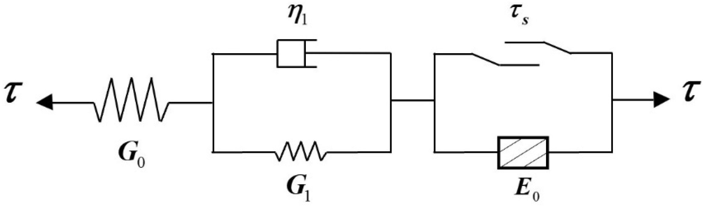
This model adopts the combination of the latter two methods, as shown in Figure 1. First, before the shear stress applied fails to reach the long-term shear strength of the joint surface, the steady material parameters in the linear model combined with the elastomer and the Kelvin model are transformed into time-dependent parameters related to factors such as time, stress, and osmotic water pressure. The deformation characteristics of rock during initial creep and steady creep are described. Then, when the joint surface reaches the long-term shear strength and is about to fail, that is, the rock joint surface enters the accelerated creep stage, at this time, a damaged body will be introduced, and the damaged body will be combined in series with the elastomer and the Kelvin model. When the damaged body is started, plastic damage begins to appear on the rock joint surface and gradually accumulates. The damage degree increases with the increase in creep time, and the damaged body also reflects that the damage intensifies with an increase in water pressure. The plastic damaged body describes the nonlinear accelerated deformation characteristics of the rock joint surface when it enters the accelerated creep stage. Through the combination of an elastomer, Kelvin model and plastic damage body, a new stress–seepage coupled shear creep model is established, which reflects the change characteristics of shear creep of rock joint surface at each stage.

The reaction shear strain in the stress–seepage coupled shear creep model mainly includes three aspects:

The first part is the instantaneous shear strain ${\gamma }_e$ expressed by the elastomer.

$${\gamma }_e={\displaystyle \frac{\tau }{G_0}}$$

(1)

where ${\gamma }_e$ is the instantaneous shear strain, $\tau$ is the shear stress, and $G_0$ is the instantaneous shear modulus.

The second part is the viscoelastic shear strain ${\gamma }_{ve}$ expressed by the Kelvin body. The Kelvin model has a simple structure and few parameters, enabling it to effectively describe the primary and secondary creep stages of rock joint surfaces, with parameters that are easy to identify from experimental data.

$${\gamma }_{ve}={\displaystyle \frac{\tau }{G_1}}(1-e^{{\displaystyle \frac{-G_1}{{\eta }_1}}t})$$

(2)

where ${\gamma }_{ve}$ is viscoelastic shear strain, $G_1$ is viscoelastic shear modulus, ${\eta }_1$ is viscoelastic viscosity coefficient, and $t$ is time.

The third part is the plastic shear strain ${\gamma }_p$ expressed by the plastic damaged body. When establishing the plastic damaged body, firstly, based on Kachanov creep damage theory, creep damage variable D is introduced to describe the change in joint surface parameters in the creep process. Damage variable D refers to the quantitative index of continuous deterioration and decreasing strength of rock materials in the creep process. Damage does not occur under any circumstances, and only when the external stress is greater than the yield stress of the rock can the damage factor of rock creep damage be established on the basis of considering the size of the external stress. Its specific manifestations are as follows:

$$D=\left\{\begin{array}{l}0,\hspace{0.33em}\hspace{0.33em}\hspace{0.33em}\hspace{0.33em}\hspace{0.33em}\hspace{0.33em}\hspace{0.33em}\hspace{0.33em}\hspace{0.33em}\hspace{0.33em}\hspace{0.33em}\hspace{0.33em}\hspace{0.33em}\hspace{0.33em}\hspace{0.33em}\hspace{0.33em}\hspace{0.33em}\hspace{0.33em}\hspace{0.33em}\hspace{0.33em}\hspace{0.33em}\hspace{0.33em}{\tau }_0<{\tau }_s\\ 1-(1-{\displaystyle \frac{t}{t_D}}{)}^{\alpha },\hspace{0.33em}\hspace{0.33em}\hspace{0.33em}\hspace{0.33em}\hspace{0.33em}\hspace{0.33em}\hspace{0.33em}\hspace{0.33em}\hspace{0.33em}\hspace{0.33em}\hspace{0.33em}{\tau }_0\ge {\tau }_s\end{array}\right.$$

(3)

where $t$ is creep time and $t_D$ is rock creep failure time, which can be estimated using some empirical models [35]. $\alpha$ is rock material parameter, ${\tau }_0$ is applied shear stress, and ${\tau }_s$ is long-term shear strength.

At the same time, under the action of seepage, the mechanical, physical and chemical effects of water aggravate the evolution of plastic damage of rock materials, so the factor of seepage water pressure is considered in the quantification of damage variables:

$$D=\left\{\begin{array}{l}0,\hspace{0.33em}\hspace{0.33em}\hspace{0.33em}\hspace{0.33em}\hspace{0.33em}\hspace{0.33em}\hspace{0.33em}\hspace{0.33em}\hspace{0.33em}\hspace{0.33em}\hspace{0.33em}\hspace{0.33em}\hspace{0.33em}\hspace{0.33em}\hspace{0.33em}\hspace{0.33em}\hspace{0.33em}\hspace{0.33em}\hspace{0.33em}\hspace{0.33em}\hspace{0.33em}{\tau }_0<{\tau }_s\\ 1-(1-{\displaystyle \frac{t}{t_D}}{)}^{\alpha P},\hspace{0.33em}\hspace{0.33em}\hspace{0.33em}\hspace{0.33em}\hspace{0.33em}\hspace{0.33em}\hspace{0.33em}\hspace{0.33em}\hspace{0.33em}{\tau }_0\ge {\tau }_s\end{array}\right.$$

(4)

where $t_D$ is rock creep failure time, $\alpha$ is rock material parameter, and $P$ is water pressure.

According to the Lemaitre strain equivalence hypothesis, the damaged element can be established as:

$${\tau }_0=E_p\cdot {\gamma }_p(1-D)$$

(5)

where $E_p$ is the deformation modulus of the damaged body. At the beginning of the damage, the deformation modulus of the damaged body will gradually decrease with the accumulation of damage, and an increase in water pressure will also aggravate the generation of damage. When the stress of the damaged body is less than the yield stress, only elastic strain is generated, and no damage is generated. Since what needs to be studied is the part of the damaged body caused by the stress exceeding the yield stress, that is, reflecting the accelerated creep stage of the rock, the constitutive model of the plastic damaged body is obtained as follows:

$${\gamma }_p=\left\{\begin{array}{l}0,\hspace{0.33em}\hspace{0.33em}\hspace{0.33em}\hspace{0.33em}\hspace{0.33em}\hspace{0.33em}\hspace{0.33em}\hspace{0.33em}\hspace{0.33em}\hspace{0.33em}\hspace{0.33em}\hspace{0.33em}\hspace{0.33em}\hspace{0.33em}\hspace{0.33em}\hspace{0.33em}\hspace{0.33em}\hspace{0.33em}\hspace{0.33em}\hspace{0.33em}\hspace{0.33em}\hspace{0.33em}{\tau }_0<{\tau }_s\\ {\displaystyle \frac{{\tau }_0}{E_p}}(1-{\displaystyle \frac{t}{t_D}}{)}^{-\alpha P},\hspace{0.33em}\hspace{0.33em}\hspace{0.33em}\hspace{0.33em}\hspace{0.33em}\hspace{0.33em}\hspace{0.33em}\hspace{0.33em}\hspace{0.33em}\hspace{0.33em}{\tau }_0\ge {\tau }_s\end{array}\right.$$

(6)

In summary, the stress–seepage coupled shear creep model is expressed as follows:

$$\gamma (t)={\gamma }_e+{\gamma }_{ve}+{\gamma }_p=\left\{\begin{array}{l}\left[{\displaystyle \frac{1}{G_0}}+{\displaystyle \frac{1}{G_1}}(1-e^{{\displaystyle \frac{-G_1}{{\eta }_1}}t})\right]{\tau }_0,\hspace{0.33em}\hspace{0.33em}\hspace{0.33em}\hspace{0.33em}\hspace{0.33em}\hspace{0.33em}\hspace{0.33em}\hspace{0.33em}\hspace{0.33em}\hspace{0.33em}\hspace{0.33em}\hspace{0.33em}\hspace{0.33em}\hspace{0.33em}\hspace{0.33em}\hspace{0.33em}\hspace{0.33em}\hspace{0.33em}\hspace{0.33em}\hspace{0.33em}\hspace{0.33em}\hspace{0.33em}{\tau }_0<{\tau }_s\\ \left[{\displaystyle \frac{1}{G_0}}+{\displaystyle \frac{1}{G_1}}(1-e^{{\displaystyle \frac{-G_1}{{\eta }_1}}t})\right]{\tau }_0+{\displaystyle \frac{{\tau }_0}{E_p}}{(1-{\displaystyle \frac{t}{t_D}})}^{-\alpha P},\hspace{0.33em}\hspace{0.33em}\hspace{0.33em}\hspace{0.33em}\hspace{0.33em}\hspace{0.33em}{\tau }_0\ge {\tau }_s\end{array}\right.$$

(7)

The stress–seepage coupled shear creep model established above is one-dimensional and needs to be derived to three-dimensional constitutive relation. In the three-dimensional stress state, the stress tensor ${\sigma }_{ij}$ of the rock can be decomposed into the partial stress tensor $S_{ij}$ and the spherical stress tensor ${\sigma }_m$. Correspondingly, the strain tensor ${\epsilon }_{ij}$ can be decomposed into the partial strain tensor $e_{ij}$ and the spherical strain tensor ${\epsilon }_m$, namely:

$$\left\{\begin{array}{l}{\sigma }_{ij}=S_{ij}+{\delta }_{ij}{\sigma }_m\\ {\epsilon }_{ij}=e_{ij}+{\delta }_{ij}{\epsilon }_m\end{array}\right.$$

(8)

where ${\delta }_{ij}$ is the Kronecker function; the spherical stress tensor and the spherical strain tensor are:

$$\left\{\begin{array}{l}{\sigma }_m={\displaystyle \frac{1}{3}}({\sigma }_1+{\sigma }_2+{\sigma }_3)={\displaystyle \frac{1}{3}}{\sigma }_{kk}\\ {\epsilon }_m={\displaystyle \frac{1}{3}}({\epsilon }_1+{\epsilon }_2+{\epsilon }_3)={\displaystyle \frac{1}{3}}{\epsilon }_{kk}\end{array}\right.$$

(9)

Then, the partial stress tensor $S_{ij}$ and the partial strain tensor $e_{ij}$ are expressed as:

$$\left\{\begin{array}{l}{S}_{ij}={\sigma }_{ij}-{\delta }_{ij}{\sigma }_m={\sigma }_{ij}-{\displaystyle \frac{1}{3}}{\sigma }_{kk}\\ e_{ij}={\epsilon }_{ij}-{\delta }_{ij}{\epsilon }_m={\epsilon }_{ij}-{\displaystyle \frac{1}{3}}{\epsilon }_{kk}\end{array}\right.$$

(10)

When the three-dimensional constitutive relation is derived from the one-dimensional model, the method of extending the one-dimensional Hooke law to the three-dimensional tensor form is usually adopted in the elastic theory. It is generally believed that the deviational stress tensor $S_{ij}$ only changes the shape of the rock but does not change the volume of the rock, and the spherical stress tensor ${\sigma }_m$ only changes the volume of the rock but does not change the shape of the rock. The following assumptions are made: First, the volume deformation of rock materials is completed in the instant of external force, and the volume deformation is elastic deformation, which does not change with the change in time; secondly, only the deviational stress tensor $S_{ij}$ can cause the creep of rock materials, and the rock materials do not creep under the action of the spherical stress tensor ${\sigma }_m$. Thirdly, Poisson’s ratio does not change during the creep process [36,37].

According to generalized Hooke’s law:

$$\left\{\begin{array}{l}{\sigma }_m=3K{\epsilon }_m\\ S_{ij}=2G{e}_{ij}\end{array}\right.$$

(11)

Among them:

$$\left\{\begin{array}{l}K={\displaystyle \frac{E}{3(1-2\mu )}}\\ G={\displaystyle \frac{E}{1+\mu }}\end{array}\right.$$

(12)

where $K$ is the volume modulus, $G$ is the shear modulus, $E$ is the elastic modulus and $\mu$ is Poisson’s ratio.

According to Formulas (4)–(7), when the applied shear stress is less than the long-term shear strength of the joint surface, that is, when $S_{ij}<S_f$:

$${\gamma }_{ij}={\gamma }_{ij}^{\mathit{e}}+{\gamma }_{ij}^{ve}={\displaystyle \frac{{\sigma }_m{\delta }_{ij}}{3K}}+{\displaystyle \frac{S_{ij}}{2G_0}}+{\displaystyle \frac{S_{ij}}{2G_1}}(1-e^{{\displaystyle \frac{-G_1}{{\eta }_1}}t})$$

(13)

where ${\gamma }_{ij}^e$ is the instantaneous shear strain described by the elastomer, ${\gamma }_{ij}^{ve}$ is the viscoelastic shear strain described by the Kelvin model, $G_0$ is the instantaneous shear modulus, $G_1$ is the viscoelastic shear modulus, and ${\eta }_1$ is the viscoelastic viscosity coefficient.

When the shear stress is greater than the long-term shear strength of the joint surface, that is, $S_{ij}\ge S_f$, the plastic damaged body is activated, and the strain tensor can be obtained by the following formula:

$${\gamma }_{ij}={\gamma }_{ij}^e+{\gamma }_{ij}^{ve}+{\gamma }_{ij}^p={\displaystyle \frac{{\sigma }_m{\delta }_{ij}}{3K}}+{\displaystyle \frac{S_{ij}}{2G_0}}+{\displaystyle \frac{S_{ij}}{2G_1}}(1-e^{{\displaystyle \frac{-G_1}{{\eta }_1}}t})+{\displaystyle \frac{S_{ij}}{E_p}}{(1-{\displaystyle \frac{t}{t_D}})}^{-\alpha P}$$

(14)

where ${\gamma }_{ij}^p$ is the strain described by the plastic damaged body and $E_p$ is the deformation modulus of the plastic damaged body.

Under this loading condition, the rock material has undergone plastic deformation and entered the viscoplastic state. The three-dimensional form for the plastic strain rate is:

$${\dot{\gamma }}_{ij}^p={\displaystyle \frac{1}{E_p}}〈\mathrm{\Phi }\left({\displaystyle \frac{F}{F_0}}\right)〉{\displaystyle \frac{\partial Q}{\partial {\sigma }_{ij}}}$$

(15)

Among them:

$$\left\{\begin{array}{l}〈\mathrm{\Phi }\left({\displaystyle \frac{F}{F_0}}\right)〉=0,\hspace{0.33em}\hspace{0.33em}\hspace{0.33em}\hspace{0.33em}\hspace{0.33em}\hspace{0.33em}\hspace{0.33em}\hspace{0.33em}\hspace{0.33em}\hspace{0.33em}\hspace{0.33em}\hspace{0.33em}\hspace{0.33em}\hspace{0.33em}\hspace{0.33em}\hspace{0.33em}\hspace{0.33em}\hspace{0.33em}F\le 0\\ 〈\mathrm{\Phi }\left({\displaystyle \frac{F}{F_0}}\right)〉=\mathrm{\Phi }\left({\displaystyle \frac{F}{F_0}}\right),\hspace{0.33em}\hspace{0.33em}\hspace{0.33em}\hspace{0.33em}\hspace{0.33em}\hspace{0.33em}\hspace{0.33em}\hspace{0.33em}\hspace{0.33em}\hspace{0.33em}\hspace{0.33em}\hspace{0.33em}F>0\end{array}\right.$$

(16)

where $F$ is the yield function of the joint plane and $F_0$ is the initial reference value of the yield function of the joint plane, which is a parameter of the same unit as $F$. $Q$ is the plastic potential function. We use the law of associated flow, that is, $F=Q$. Some studies found through experiments that the $\mathrm{\Phi }$ function can be expressed as a power function; combined with the associated flow rule, then:

$${\dot{\gamma }}_{ij}^p={\displaystyle \frac{1}{E_p}}{\left({\displaystyle \frac{F}{F_0}}\right)}^M{\displaystyle \frac{\partial F}{\partial {\sigma }_{ij}}}$$

(17)

where $M$ is the rock material parameter, generally taken as 1.

Finally, the three-dimensional creep model of the rock joint surface can be expressed as:

$$\left\{\begin{array}{l}{\gamma }_{ij}={\displaystyle \frac{{\sigma }_m{\delta }_{ij}}{3K}}+{\displaystyle \frac{S_{ij}}{2G_0}}+{\displaystyle \frac{S_{ij}}{2G_1}}(1-e^{{\displaystyle \frac{-G_1}{{\eta }_1}}t}),\hspace{0.33em}\hspace{0.33em}\hspace{0.33em}\hspace{0.33em}\hspace{0.33em}\hspace{0.33em}\hspace{0.33em}\hspace{0.33em}\hspace{0.33em}\hspace{0.33em}\hspace{0.33em}\hspace{0.33em}\hspace{0.33em}\hspace{0.33em}\hspace{0.33em}\hspace{0.33em}\hspace{0.33em}\hspace{0.33em}\hspace{0.33em}\hspace{0.33em}\hspace{0.33em}\hspace{0.33em}\hspace{0.33em}\hspace{0.33em}\hspace{0.33em}\hspace{0.33em}\hspace{0.33em}F<0\\ {\gamma }_{ij}={\displaystyle \frac{{\sigma }_m{\delta }_{ij}}{3K}}+{\displaystyle \frac{S_{ij}}{2G_0}}+{\displaystyle \frac{S_{ij}}{2G_1}}(1-e^{{\displaystyle \frac{-G_1}{{\eta }_1}}t})+{\displaystyle \frac{1}{E_p}}{(1-{\displaystyle \frac{t}{t_D}})}^{-\alpha P}\left({\displaystyle \frac{F}{F_0}}\right),\hspace{0.33em}\hspace{0.33em}\hspace{0.33em}\hspace{0.33em}\hspace{0.33em}\hspace{0.33em}F\ge 0\end{array}\right.$$

(18)

Under the action of direct shear stress, the shear creep model of rock joint surface can be further expressed as:

$$\begin{array}{l}\gamma (t)=\left[{\displaystyle \frac{1}{G_0}}+{\displaystyle \frac{1}{G_1}}(1-e^{{\displaystyle \frac{-G_1}{{\eta }_1}}t})\right]\tau ,\hspace{0.33em}\hspace{0.33em}\hspace{0.33em}\hspace{0.33em}\hspace{0.33em}\hspace{0.33em}\hspace{0.33em}\hspace{0.33em}\hspace{0.33em}\hspace{0.33em}\hspace{0.33em}\hspace{0.33em}\hspace{0.33em}\hspace{0.33em}\hspace{0.33em}\hspace{0.33em}\hspace{0.33em}\hspace{0.33em}\hspace{0.33em}\hspace{0.33em}\hspace{0.33em}\tau <{\tau }_s\\ \gamma (t)=\left[{\displaystyle \frac{1}{G_0}}+{\displaystyle \frac{1}{G_1}}(1-e^{{\displaystyle \frac{-G_1}{{\eta }_1}}t})\right]\tau +{\displaystyle \frac{\tau }{E_p}}{(1-{\displaystyle \frac{t}{t_D}})}^{-\alpha P},\hspace{0.33em}\hspace{0.33em}\hspace{0.33em}\hspace{0.33em}\hspace{0.33em}\tau \ge {\tau }_s\end{array}$$

(19)

where $\gamma$ is the shear strain, $G_0$ is the instantaneous shear modulus, $G_1$ is the viscoelastic shear modulus, ${\eta }_1$ is the viscoelastic viscosity coefficient, $E_p$ is the deformation modulus of the plastic damaged body, $t$ is the creep time, $t_D$ is the creep failure time of the rock joint surface, $\alpha$ is the material parameter, $P$ is the water pressure, $\tau$ is the shear stress, and ${\tau }_s$ is the long-term shear strength of the rock joint surface.

3. The Establishment of the Shear Creep Model

3.1. Calculation of Effective Shear Stress

In the process of shear creep of artificial rock joints with regular serrated teeth under the coupled condition of stress and seepage flow, the external shear stress exerted by the artificial rock joints with regular serrated teeth not only overcomes the cohesion force of the joint teeth but also needs to overcome the friction force of the joint surface. Therefore, the actual effective shear stress exerted on the serrated joint plane should be the difference between the applied shear stress load and the friction resistance of the joint surface, namely:

$$\tilde{\tau }={\tau }_0-f\times {\sigma }_{ne}$$

(20)

where $\tilde{\tau }$ is the effective shear stress, $f$ is the friction coefficient of the joint surface, ${\sigma }_{ne}$ is the normal effective stress of the joint surface, and ${\tau }_0$ is the applied shear stress load.

According to the principle of effective stress, the effective normal stress of the joint surface can be obtained according to the following formula:

$${\sigma }_{ne}={\sigma }_n-\alpha P$$

(21)

where ${\sigma }_n$ is the normal stress load applied, $P$ is the water pressure of the joint surface, and $\alpha$ is the Biot coefficient. Because the sample is a through-crack, the $\alpha$ is 1.

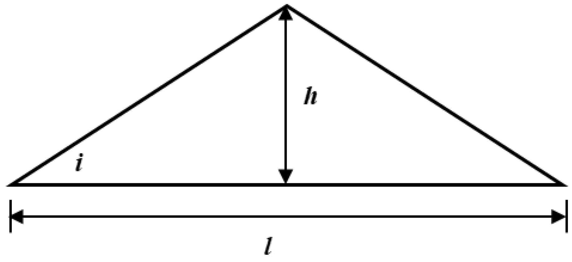
For the regular toothed joint surface, as shown in Figure 2, the equivalent friction angle in the shearing process is the sum of the basic friction angle and the joint fluctuation angle, which is calculated as follows:

$${\varphi }_e={\varphi }_j+i$$

(22)

where ${\varphi }_e$ is the equivalent friction angle, ${\varphi }_j$ is the basic friction angle, $i$ is the undulation angle, $i=\arctan {\displaystyle \frac{h}{l/2}}$, and respectively, $h,l$ are the height and bottom edge length of a single sawtooth.

In this way, the friction coefficient of the joint surface can be calculated:

$$f=\tan {\varphi }_e$$

(23)

Therefore, the effective shear stress under the stress–seepage coupling condition can be calculated by the following formula:

$$\tilde{\tau }={\tau }_0-\tan ({\varphi }_j+\arctan {\displaystyle \frac{h}{l/2}})\times ({\sigma }_n-P)$$

(24)

where $\tilde{\tau }$ is the effective shear stress, ${\tau }_0$ is the actual applied shear stress load, ${\varphi }_j$ is the basic friction angle, $h,l$ are the height of a single sawtooth on the joint surface and the length of the bottom edge, ${\sigma }_n$ is the applied normal stress load, and $P$ is the water pressure on the joint surface.

3.2. The Solution of Creep Parameters

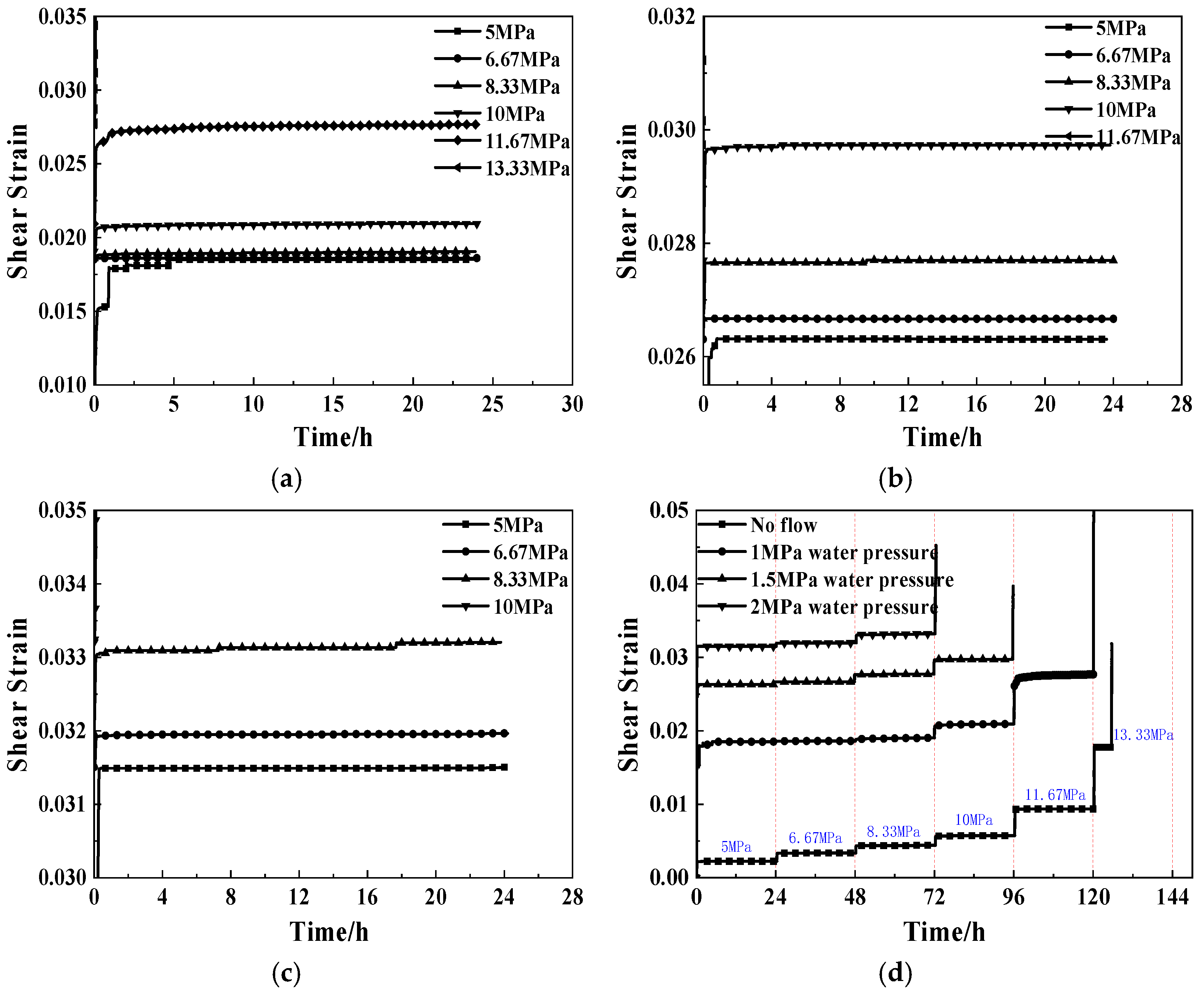
In previous research, considering the actual stress conditions and groundwater occurrence states experienced by joints during the creep process in practical engineering, a series of shear creep tests were conducted on specimens containing through-saw-toothed joints [38]. These tests investigated the hydro-mechanical coupled shear creep characteristics of joints with different degrees of roughness. Furthermore, the influences of joint asperity height, normal stress, and water pressure on the shear creep behavior, long-term shear strength, shear creep rate, dilatancy characteristics, and seepage properties of the joints were evaluated. As shown in Figure 3, an abundance of experimental data and curves was obtained through the tests, providing reliable data support for establishing a stress–seepage coupled shear creep model for rock joints.

The values of various creep parameters in the initial creep stage and the steady creep stage are constantly changing with changes in time, effective shear stress, and osmotic water pressure. Therefore, the changing trends of the instantaneous elastic modulus $G_0$, viscoelastic shear modulus $G_1$, and viscoelastic viscosity coefficient ${\eta }_1$ with time, effective shear stress, and osmotic pressure will be analyzed next.

Based on the experimental data of the coupled shear creep under water pressures of 0, 1 MPa, 1.5 MPa and 2 MPa, the creep parameters were studied. According to the method of calculating effective shear stress, the shear stress at all levels under each working condition was calculated, and the statistics are shown in

Table 1. Test cases.

	Fluctuation Heights/mm	Normal Stress/MPa	Water Pressure/MPa	Effective Shear Stress/MPa
Case 1	6	5	0	1.69, 3.36, 5.02, 6.69, 8.36
Case 2			1	2.35, 4.02, 5.68, 7.35, 9.02
Case 3			1.5	2.68, 4.35, 6.01, 7.68
Case 4			2	3.01, 4.68, 6.34

.

Under constant stress, creep parameters are only time-dependent. Before reaching the accelerated creep stage, 0.5 h, 4 h, 8 h, 12 h, 16 h, 20 h, and 24 h were taken as the analysis time nodes under the effective shear stress of each stage. The creep parameters are considered to remain constant in the inter-cell area around each time. In this interval, 10 groups of test data are taken, and the creep parameters at each time are obtained by Origin-2018 software with the nonlinear least square method [39,40]. According to this method, creep parameters at different times can be obtained and the relationship between parameters and time can be analyzed. According to the creep parameters under different effective shear stresses at the same initial time, the relationship between parameters and effective shear stress can be analyzed.

Table 2. Statistics of creep parameters of Case 1 under the action of effective shear stress at all levels.

Effective Shear Stress/MPa	Time/h	${\mathit{G}}_0$$\mathbf{/}\mathbf{G}\mathbf{P}\mathbf{a}$	${\mathit{G}}_1$$/GPa$	${\mathit{\eta }}_1$$/GPa·h$
1.69	0.5	6.618	1.042	0.025
	4	6.618	0.922	0.084
	8	6.618	0.857	0.195
	12	6.618	0.857	0.293
	16	6.618	0.857	0.392
	20	6.618	0.857	0.496
	24	6.618	0.857	0.592
3.36	0.5	13.167	1.486	0.040
	4	13.167	1.203	0.128
	8	13.167	1.083	0.241
	12	13.167	1.083	0.370
	16	13.167	1.083	0.495
	20	13.167	1.083	0.628
	24	13.167	1.083	0.754
5.02	0.5	19.676	1.712	0.054
	4	19.676	1.438	0.148
	8	19.676	1.218	0.276
	12	19.676	1.218	0.419
	16	19.676	1.218	0.560
	20	19.676	1.203	0.693
	24	19.676	1.203	0.846
6.69	0.5	26.226	1.922	0.071
	4	26.226	1.604	0.149
	8	26.226	1.359	0.302
	12	26.226	1.356	0.462
	16	26.226	1.356	0.631
	20	26.226	1.343	0.777
	24	26.226	1.338	0.933
8.36	0.5	32.775	2.228	0.090
	4	32.775	1.813	0.198
	8	32.775	1.617	0.367
	12	32.775	1.617	0.553
	16	32.775	1.617	0.747
	20	32.775	1.595	0.923
	24	32.775	1.595	1.105

,

Table 3. Statistics of creep parameters of Case 2 under the action of effective shear stress at all levels.

Effective Shear Stress/MPa	Time/h	${\mathit{G}}_0$$/GPa$	${\mathit{G}}_1$$/GPa$	${\mathit{\eta }}_1$$/GPa·\mathbf{h}$
2.35	0.5	4.519	0.191	0.007
	4	4.519	0.158	0.017
	8	4.519	0.153	0.038
	12	4.519	0.153	0.052
	16	4.519	0.153	0.071
	20	4.519	0.153	0.089
	24	4.519	0.153	0.108
4.02	0.5	7.731	0.274	0.011
	4	7.731	0.245	0.027
	8	7.731	0.239	0.054
	12	7.731	0.238	0.082
	16	7.731	0.238	0.111
	20	7.731	0.238	0.139
	24	7.731	0.238	0.167
5.68	0.5	10.923	0.338	0.016
	4	10.923	0.316	0.035
	8	10.923	0.309	0.069
	12	10.923	0.308	0.105
	16	10.923	0.307	0.142
	20	10.923	0.307	0.179
	24	10.923	0.307	0.214
7.35	0.5	14.135	0.399	0.020
	4	14.135	0.373	0.041
	8	14.135	0.364	0.083
	12	14.135	0.362	0.124
	16	14.135	0.362	0.167
	20	14.135	0.361	0.209
	24	14.135	0.360	0.250
9.02	0.5	17.346	0.461	0.023
	4	17.346	0.427	0.046
	8	17.346	0.423	0.095
	12	17.346	0.417	0.138
	16	17.346	0.417	0.191
	20	17.346	0.417	0.240
	24	17.346	0.417	0.288

,

Table 4. Statistics of creep parameters of Case 3 under the action of effective shear stress at all levels.

Effective Shear Stress/MPa	Time/h	${\mathit{G}}_0$$/GPa$	${\mathit{G}}_1$$/GPa$	${\mathit{\eta }}_1$$/GPa·\mathbf{h}$
2.68	0.5	2.668	0.122	0.003
	4	2.668	0.114	0.012
	8	2.668	0.106	0.024
	12	2.668	0.106	0.036
	16	2.668	0.106	0.048
	20	2.668	0.106	0.061
	24	2.668	0.106	0.074
4.35	0.5	4.330	0.198	0.009
	4	4.330	0.184	0.020
	8	4.330	0.169	0.038
	12	4.330	0.169	0.057
	16	4.330	0.169	0.078
	20	4.330	0.169	0.098
	24	4.330	0.169	0.118
6.01	0.5	5.981	0.257	0.013
	4	5.981	0.235	0.027
	8	5.981	0.225	0.050
	12	5.981	0.225	0.076
	16	5.981	0.225	0.104
	20	5.981	0.225	0.130
	24	5.981	0.225	0.155
7.68	0.5	7.643	0.318	0.018
	4	7.643	0.288	0.037
	8	7.643	0.268	0.060
	12	7.643	0.267	0.091
	16	7.643	0.267	0.122
	20	7.643	0.267	0.153
	24	7.643	0.267	0.183

and

Table 5. Statistics of creep parameters of Case 4 under the action of effective shear stress at all levels.

Effective Shear Stress/MPa	Time/h	${\mathit{G}}_0$$/GPa$	${\mathit{G}}_1$$/GPa$	${\mathit{\eta }}_1$$/GPa·\mathbf{h}$
3.01	0.5	1.581	0.119	0.003
	4	1.581	0.109	0.012
	8	1.581	0.102	0.023
	12	1.581	0.102	0.035
	16	1.581	0.102	0.047
	20	1.581	0.102	0.059
	24	1.581	0.102	0.071
4.68	0.5	2.458	0.182	0.004
	4	2.458	0.167	0.017
	8	2.458	0.156	0.035
	12	2.458	0.156	0.053
	16	2.458	0.156	0.072
	20	2.458	0.156	0.091
	24	2.458	0.156	0.108
6.34	0.5	3.329	0.231	0.007
	4	3.329	0.214	0.024
	8	3.329	0.200	0.045
	12	3.329	0.200	0.069
	16	3.329	0.200	0.092
	20	3.329	0.200	0.116
	24	3.329	0.199	0.138

show the creep parameters at different times of the samples under effective shear stresses of 0, 1 MPa, 1.5 MPa, and 2 MPa, respectively.

3.3. The Evolutionary Law of Creep Parameters

According to the creep parameters obtained in the previous section, corresponding nonlinear functions can be customized according to the selected shear creep model, and mathematical expressions of creep parameters and influencing factors can be obtained by the nonlinear curve fitting method [39]. To obtain the values of other arbitrary time parameters according to the creep parameters of the initial time in the fitting expression, the relationship between the parameters of any time and the initial time parameters is often used to fit. Moreover, from the point of view of damage mechanics, establishing the relationship between the initial time and the creep parameters at any time also reflects the damage process of material properties with time. According to the test results, 0.5 h will be used as the initial time in the following paragraphs. In addition, when studying the change law of creep parameters, it is often necessary to fit the combination of the desired parameters and other variables (such as time) so that the fitting curve obtained is more accurate and the fitting function relationship is more intuitive.

3.3.1. Variation in Creep Parameters with Time

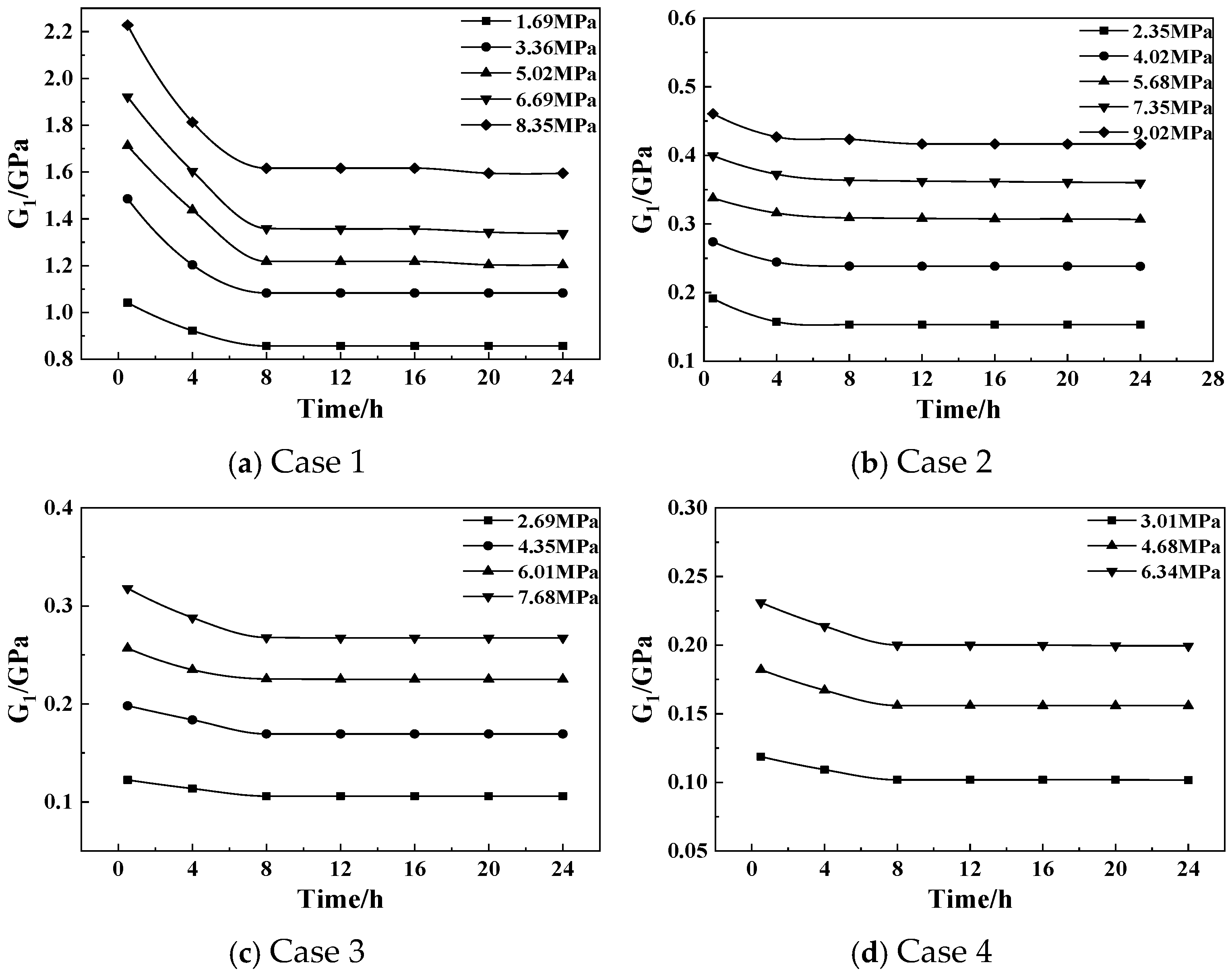
The ratio of shear stress to corresponding instantaneous shear strain in creep tests is defined as the instantaneous elastic shear modulus, so the instantaneous elastic shear modulus has almost no correlation with time. The change in the law of the instantaneous shear modulus with time is not discussed. Figure 4 shows the variation in the viscoelastic shear modulus of the sample with time under different shear stresses under four working conditions. As can be seen from Figure 4, the viscoelastic shear modulus gradually decreases with the extension of creep time and eventually becomes stable. Because the viscoelastic shear modulus determines the limit value of viscoelastic deformation, that is, $S_{ij}/2G_1$, it can be seen from the shear creep test curve that in the process of the shear creep test, with the increase in shear creep time, the viscoelastic deformation will increase to a fixed value and then remain basically unchanged, so the viscoelastic shear modulus gradually decreases with the creep time and finally tends to a fixed value.

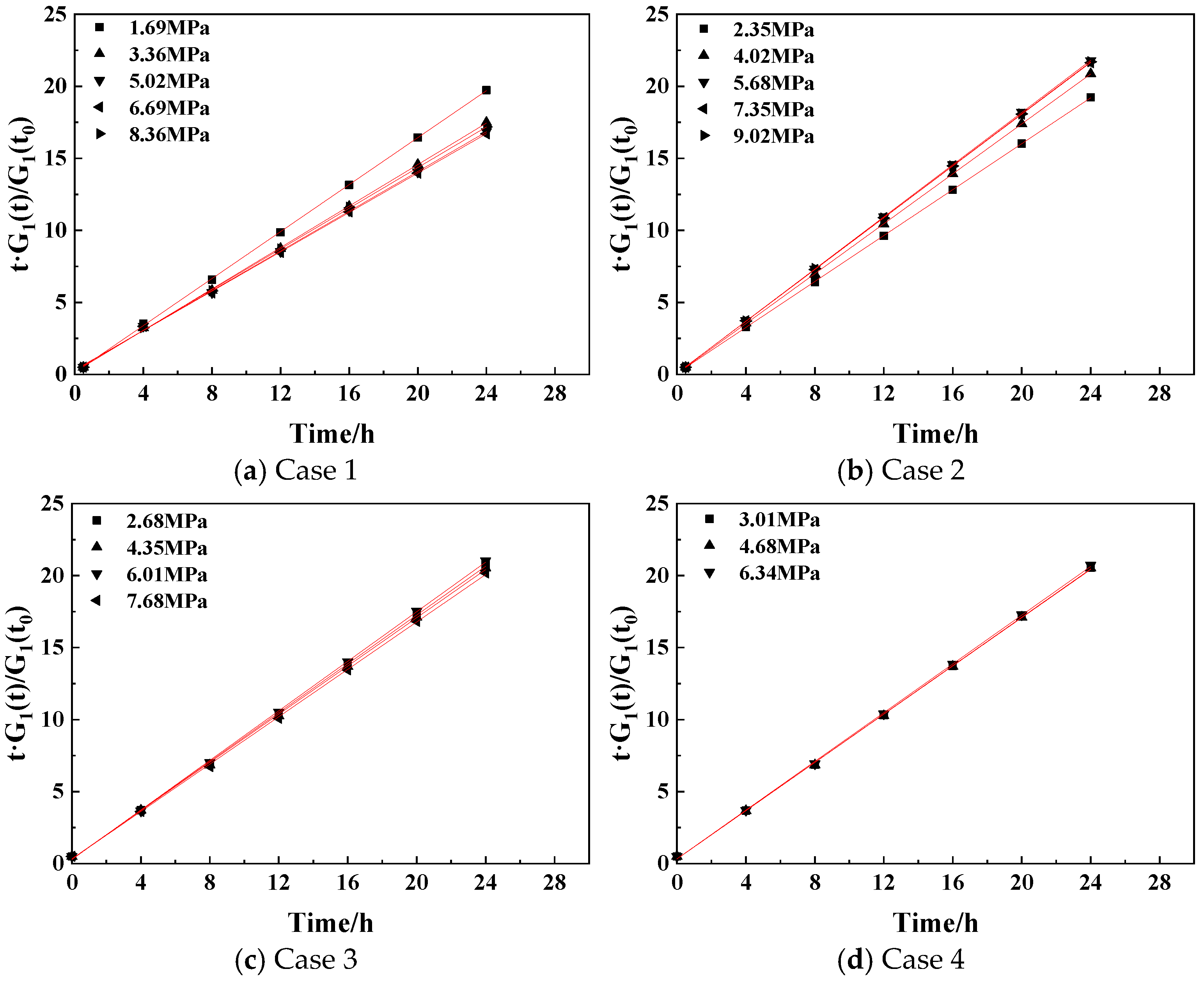
To facilitate the analysis, with a more intuitive and accurate fitting function, $t\times G_1(t)/G_1(t_0)$ is used as the function relationship and change rule between the dependent variable and the independent variable time. It can be seen from Figure 5 that $t\times G_1(t)/G_1(t_0)$ increases linearly with the creep time.

According to data fitting, the relationship between viscoelastic shear modulus and creep time is as follows:

$$t\times G_1(t)/G_1(t_0)=a+b\times t$$

(25)

Then,

$$G_1(t)=G_1(t_0)({\displaystyle \frac{a}{t}}+b)$$

(26)

where $G_1(t)$ is the viscoelastic shear modulus at any time, $G_1(t_0)$ is the viscoelastic shear modulus at the initial time, $t$ is time, where t_min is taken as the starting time of experimental data acquisition (t_min = 0.5 h) in the paper, and $a$, $b$ is the fitting parameter. The fitting coefficient and fitting degree statistics of the viscoelastic shear modulus with time are shown in

Table 6. Fitting coefficient between $t\times G_1(t)/G_1(t_0)$ and $t$.

	Effective Shear Stress/MPa	a	b	Degree of Fitting	F	p
Case 1	1.69	0.133	0.815	0.999	4995	<0.05
	3.36	0.181	0.719	0.999
	5.02	0.306	0.689	0.999
	6.69	0.315	0.683	0.999
	8.35	0.251	0.705	0.999
Case 2	2.35	0.081	0.797	0.999
	4.02	0.066	0.866	0.999
	5.68	0.081	0.905	0.999
	7.35	0.095	0.898	0.999
	9.02	0.085	0.9	0.999
Case 3	2.68	0.321	0.847	0.999
	4.35	0.335	0.837	0.999
	6.01	0.289	0.86	0.999
	7.68	0.327	0.823	0.999
Case 4	3.01	0.332	0.846	0.999
	4.68	0.323	0.838	0.999
	6.34	0.327	0.839	0.999

. According to the fitting results, this functional relationship can well represent the change law of viscoelastic shear modulus with time. Performing an F-test on the fitting results, a p-value of less than 0.05 indicates that the fitting is statistically significant.

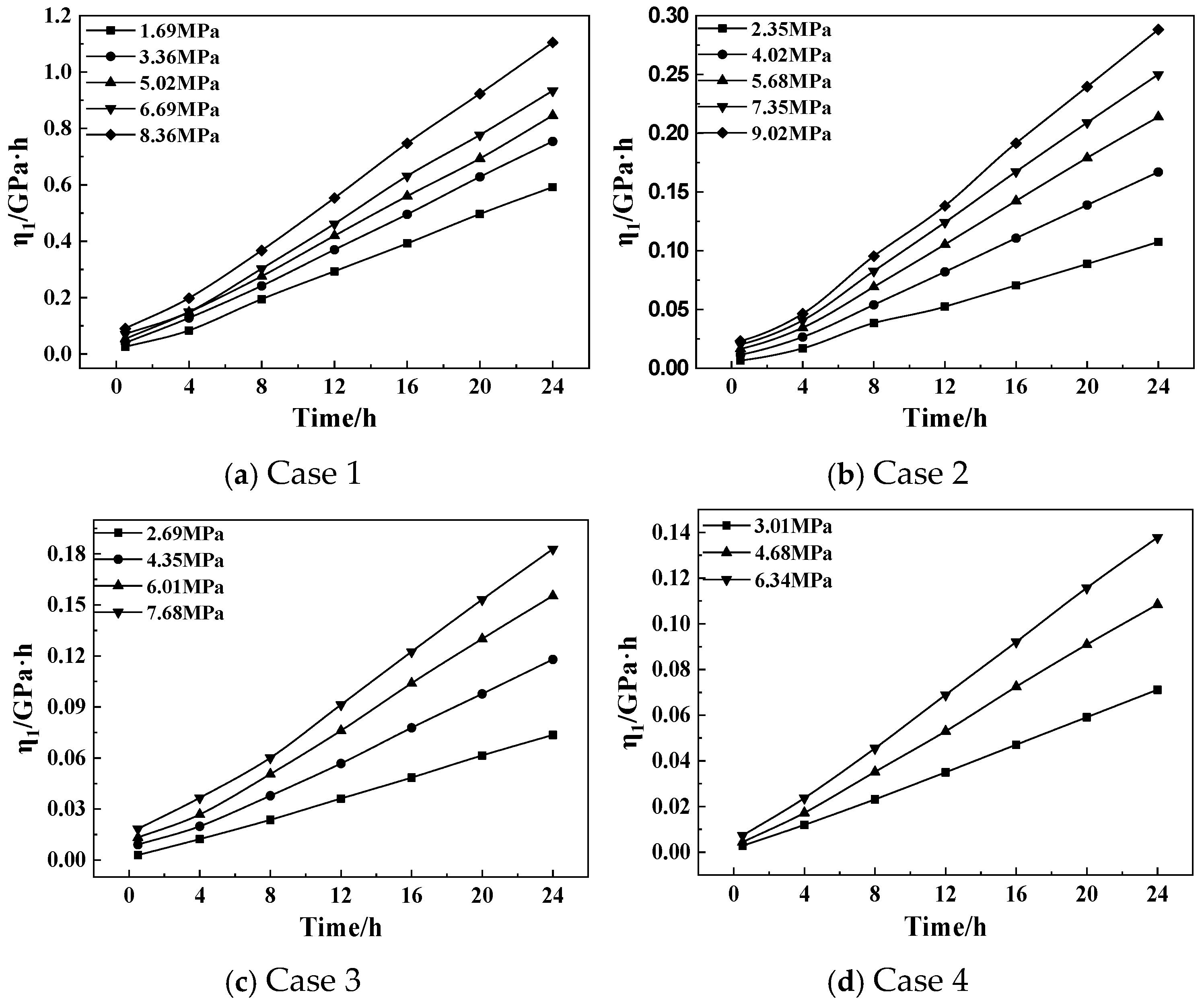
Figure 6 shows the change in the viscoelastic viscosity coefficient of the sample with time under different shear stresses and four different working conditions. As can be seen from Figure 6, the viscoelastic viscosity coefficient basically increases linearly with the extension of time. It can be seen from the creep equation that the length of time to reach the stability stage is determined by the size of the viscoelastic viscosity coefficient. When the time tends to infinity, the viscoelastic deformation of the sample tends to a fixed value. As can be seen from the above, when $G_1$ tends to a fixed value, ${\eta }_1$ should change in a linear relationship with time, and its slope should be fixed.

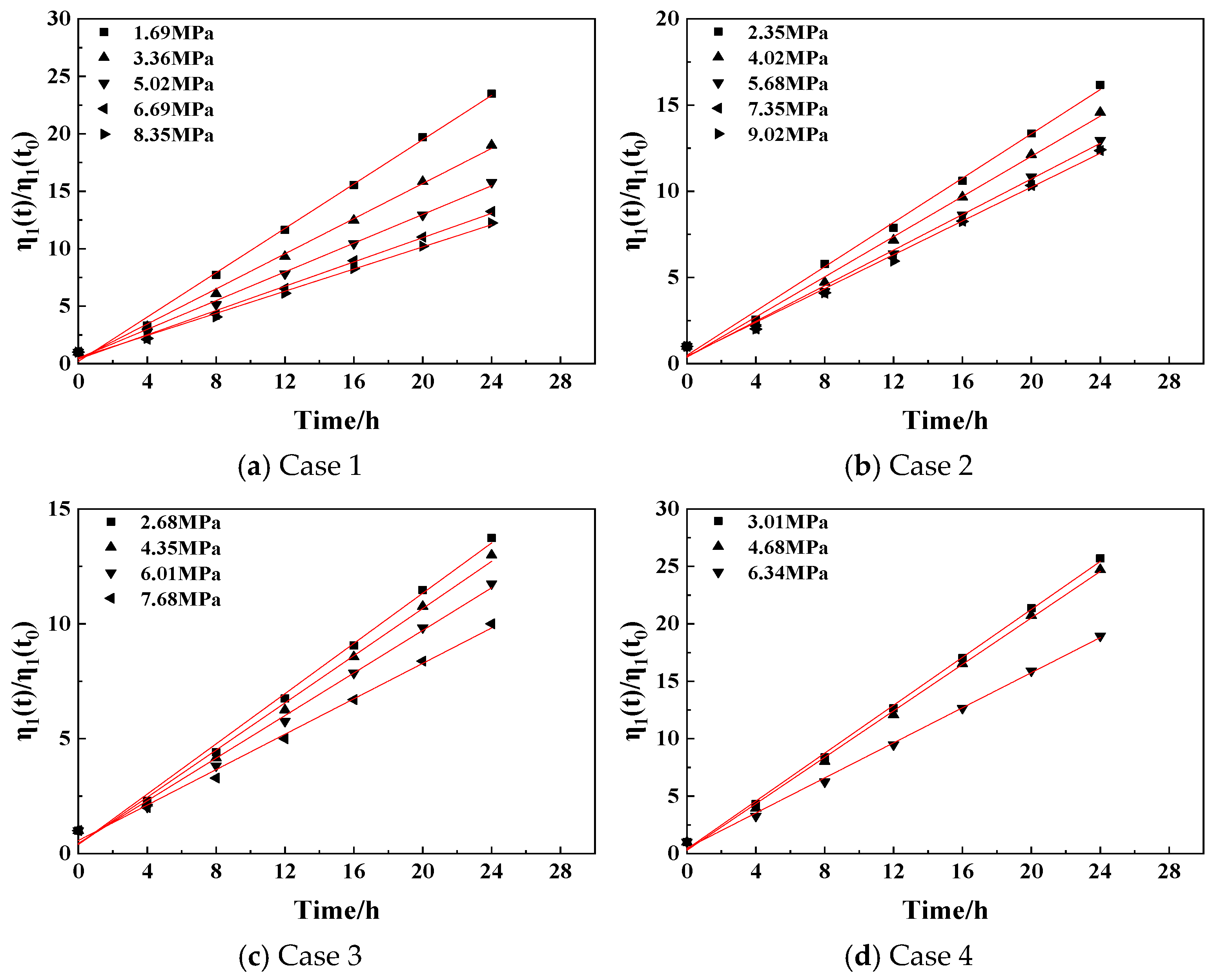
As shown in Figure 7, ${\eta }_1(t)/{\eta }_1(t_0)$ is used as the dependent variable to analyze the functional relationship and change rule between the independent variable times. It can be seen from Figure 7 that ${\eta }_1(t)/{\eta }_1(t_0)$ increases linearly with the creep time.

According to data fitting, the relationship between the viscoelastic viscosity coefficient and creep time is as follows:

$${\eta }_1(t)/{\eta }_1(t_0)=a+bt$$

(27)

Then,

$${\eta }_1(t)={\eta }_1(t_0)\times (a+bt)$$

(28)

where ${\eta }_1(t)$ is the viscoelastic viscosity coefficient at any time, ${\eta }_1(t_0)$ is the viscoelastic viscosity coefficient at the initial time, $t$ is time, and $a$, $b$ is the fitting parameter. The fitting coefficient of the viscoelastic viscosity coefficient with time and the fitting degree statistics are shown in

Table 7. Fitting coefficient between viscoelastic ${\eta }_1(t)/{\eta }_1(t_0)$ and $t$.

	Effective Shear Stress/MPa	a	b	Degree of Fitting	F	p
Case 1	1.69	0.195	0.965	0.999	4995	<0.05
	3.36	0.388	0.764	0.999
	5.02	0.785	0.625	0.999
	6.69	0.396	0.528	0.999
	8.35	0.52	0.482	0.999
Case 2	2.35	0.486	0.642	0.999
	4.02	0.373	0.583	0.999
	5.68	0.393	0.516	0.999
	7.35	0.432	0.49	0.999
	9.02	0.398	0.491	0.999
Case 3	2.68	0.401	0.547	0.999
	4.35	0.396	0.513	0.999
	6.01	0.445	0.463	0.999
	7.68	0.569	0.385	0.999
Case 4	3.01	0.396	1.043	0.999
	4.68	0.292	1.011	0.999
	6.34	0.477	0.763	0.999

. According to the fitting results, this functional relationship can well represent the change in the viscoelastic viscosity coefficient with time. Performing an F-test on the fitting results, a p-value of less than 0.05 indicates that the fitting is statistically significant.

3.3.2. Variation in Creep Parameters with Effective Shear Stress

According to the relationship between creep parameters and effective shear stress, the mathematical expression of creep parameters and effective shear stress can be obtained by the nonlinear curve fitting method. The change of law of each creep parameter and effective shear stress at the initial time is solved below. With t = 0.5 h, $G_0$, $G_1$, and ${\eta }_1$ as the initial values, the variation laws of the three parameters with different shear stresses under different working conditions were obtained.

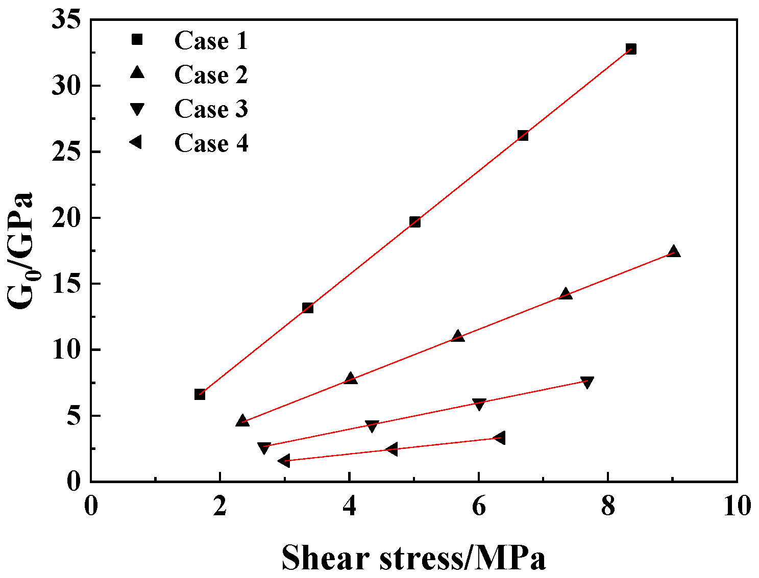
As shown in Figure 8, according to data fitting, the relationship between instantaneous elastic shear modulus and shear stress is as follows:

$$G_0=a\times \tau$$

(29)

where $G_0$ is the instantaneous elastic shear modulus, $\tau$ is the effective shear stress, and $a$, $b$, $c$ is the fitting parameter. The fitting coefficient and fitting degree statistics of the instantaneous elastic shear modulus and effective shear stress are shown in

Table 8. Fitting coefficient between viscoelastic shear modulus and effective shear stress.

	Case 1	Case 2	Case 3	Case 4
a	3.922	1.923	0.995	0.525
Degree of fitting	0.999	0.999	0.999	0.999
F	2997	2997	1998	999
p	<0.05

. According to the fitting results, this functional relationship can well represent the change in the instantaneous elastic shear modulus with effective shear stress. Performing an F-test on the fitting results, a p-value of less than 0.05 indicates that the fitting is statistically significant.

As shown in Figure 9, according to the data fitting, the relationship between the initial viscoelastic shear modulus (when t = 0.5 h) and the effective shear stress is as follows:

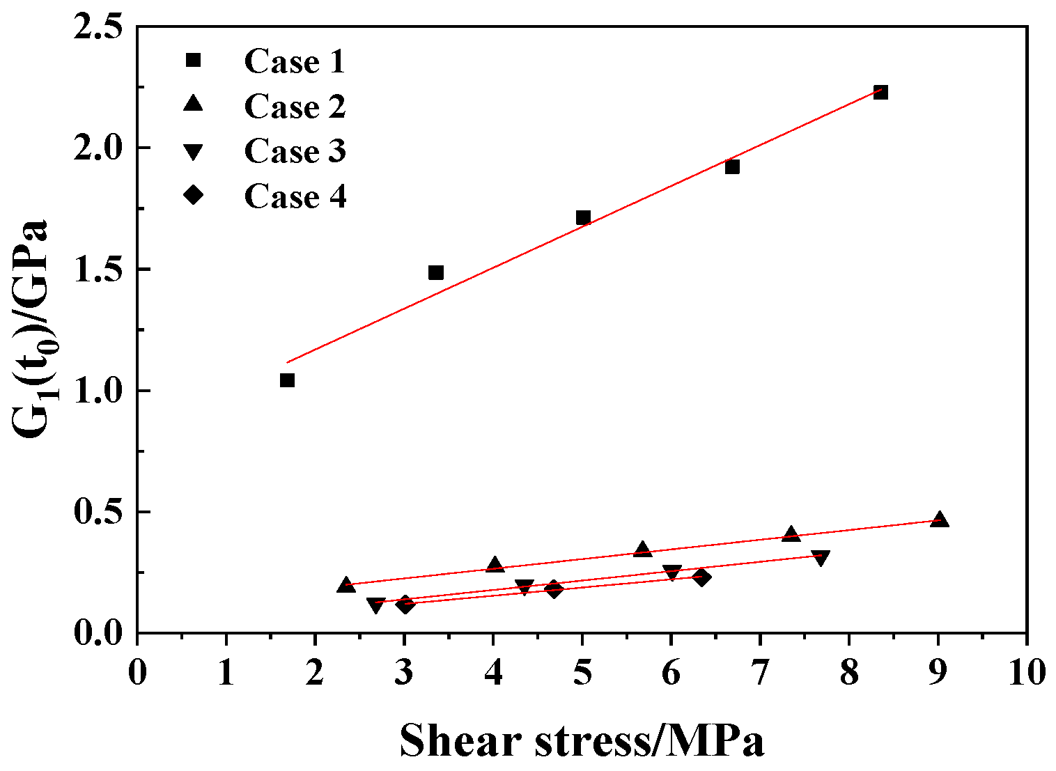
$$G_1(t_0)=a+b\tau$$

(30)

where $G_1(t_0)$ is the viscoelastic shear modulus at the initial moment, $\tau$ is the effective shear stress, and $a$, $b$ is the fitting parameter. The fitting coefficient and fitting degree statistics of the initial viscoelastic shear modulus and effective shear stress are shown in

Table 9. Fitting coefficient between initial viscoelastic shear modulus and effective shear stress.

	Case 1	Case 2	Case 3	Case 4
a	0.832	0.106	0.023	0.019
b	0.169	0.040	0.039	0.034
Degree of fitting	0.981	0.996	0.997	0.997
F	155	747	665	332
p	<0.05

. According to the fitting results, this functional relationship can well represent the change in the initial viscoelastic shear modulus with effective shear stress. Performing an F-test on the fitting results, a p-value of less than 0.05 indicates that the fitting is statistically significant.

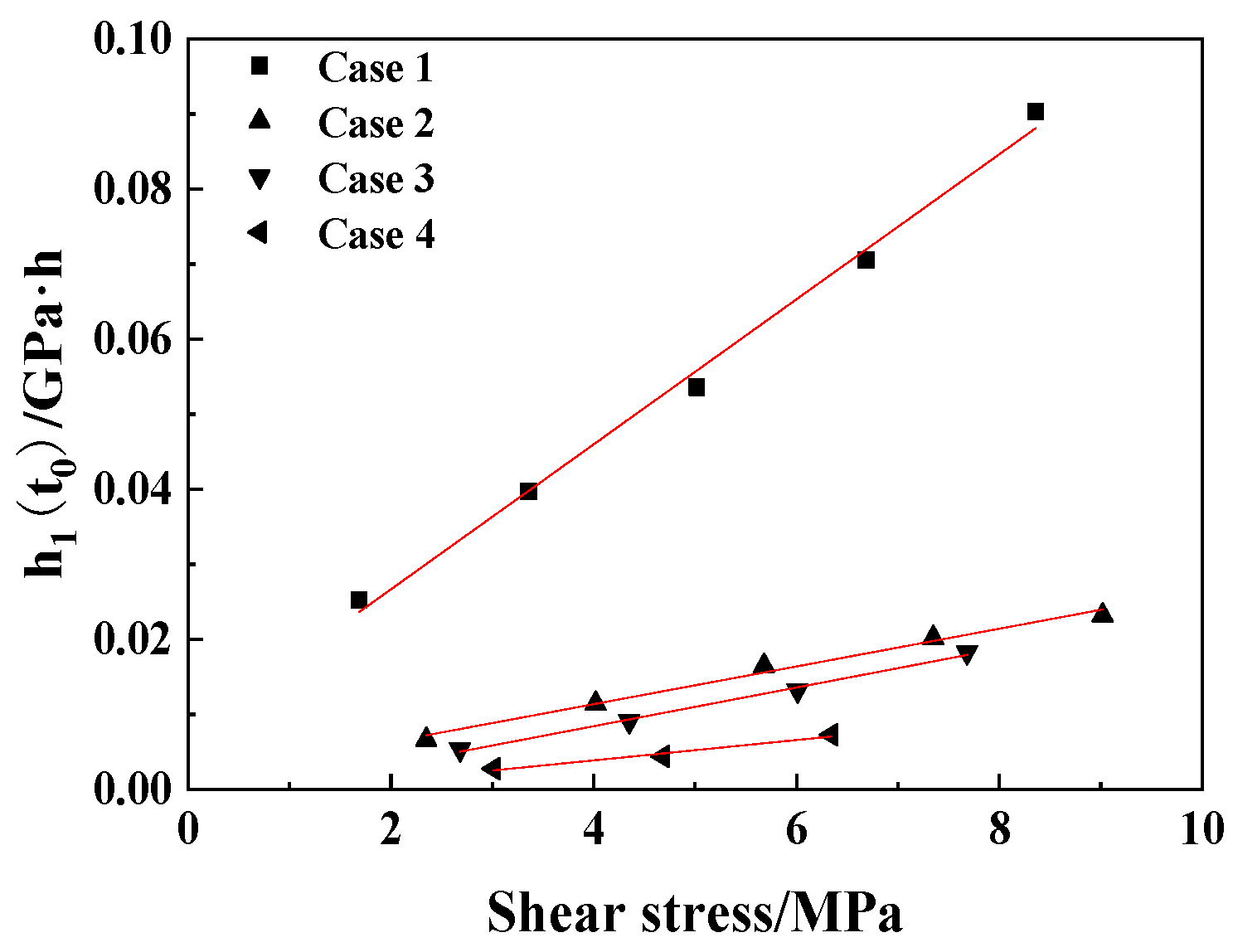
As shown in Figure 10, according to data fitting, the relationship between the initial viscoelastic viscosity coefficient (t = 0.5 h) and the effective shear stress is as follows:

$${\eta }_1(t_0)=a+b\tau$$

(31)

where ${\eta }_1(t_0)$ is the viscoelastic viscosity coefficient at the initial time, $\tau$ is the effective shear stress, and $a$, $b$ is the fitting parameter.

The fitting coefficient and fitting degree statistics of the initial viscoelastic viscosity coefficient and effective shear stress are shown in

Table 10. Fitting coefficient between initial viscoelastic viscosity coefficient and effective shear stress.

	Case 1	Case 2	Case 3	Case 4
a	0.0074	0.0013	−0.0019	−0.0015
b	0.0097	0.0025	0.0026	0.0014
Degree of fitting	0.995	0.989	0.995	0.997
F	597	270	398	332
p	<0.05

. According to the fitting results, this functional relationship can well represent the change law of the initial viscoelastic viscosity coefficient with effective shear stress. Performing an F-test on the fitting results, a p-value of less than 0.05 indicates that the fitting is statistically significant.

3.3.3. Variation in Creep Parameters with Water Pressure

To facilitate the analysis, the magnitude of the initial creep parameter under the same effective shear stress under different water pressure conditions can be obtained according to this change law, and then the influence law of seepage water pressure on the creep parameter at the initial time can be compared and analyzed. The deterioration of seepage on creep parameters can be expressed by seepage damage variables, which are defined as follows:

$$D_P=\left\{\begin{array}{l}0,\hspace{0.33em}\hspace{0.33em}\hspace{0.33em}\hspace{0.33em}\hspace{0.33em}\hspace{0.33em}\hspace{0.33em}\hspace{0.33em}\hspace{0.33em}\hspace{0.33em}\hspace{0.33em}\hspace{0.33em}\hspace{0.33em}\hspace{0.33em}\hspace{0.33em}P=0\\ 1-M_P/M_0,\hspace{0.33em}\hspace{0.33em}\hspace{0.33em}\hspace{0.33em}\hspace{0.33em}\hspace{0.33em}P>0\end{array}\right.$$

(32)

where $M_0$ is the creep parameter under the condition of no water, $M_P$ is the creep parameter after seepage damage and deterioration under arbitrary water pressure, and $P$ is the water pressure.

The above is a general representation of seepage damage variables, which may be expressed in different ways for each creep parameter. The following is the specific expression of the instantaneous elastic shear modulus, viscoelastic shear modulus and viscoelastic viscosity coefficient for seepage damage variables through the analysis and fitting of test data.

The seepage damage variable of the instantaneous elastic shear modulus can be expressed as:

$$D_P=\left\{\begin{array}{l}0,\hspace{0.33em}\hspace{0.33em}\hspace{0.33em}\hspace{0.33em}\hspace{0.33em}\hspace{0.33em}\hspace{0.33em}\hspace{0.33em}\hspace{0.33em}\hspace{0.33em}\hspace{0.33em}\hspace{0.33em}\hspace{0.33em}\hspace{0.33em}\hspace{0.33em}\hspace{0.33em}\hspace{0.33em}\hspace{0.33em}\hspace{0.33em}\hspace{0.33em}\hspace{0.33em}\hspace{0.33em}\hspace{0.33em}\hspace{0.33em}\hspace{0.17em}\hspace{0.17em}P=0\\ 1-G_0(P)/G_0(0),\hspace{0.33em}\hspace{0.33em}\hspace{0.33em}\hspace{0.33em}\hspace{0.33em}\hspace{0.33em}\hspace{0.33em}\hspace{0.33em}\hspace{0.33em}\hspace{0.33em}\hspace{0.33em}\hspace{0.33em}P>0\end{array}\right.$$

(33)

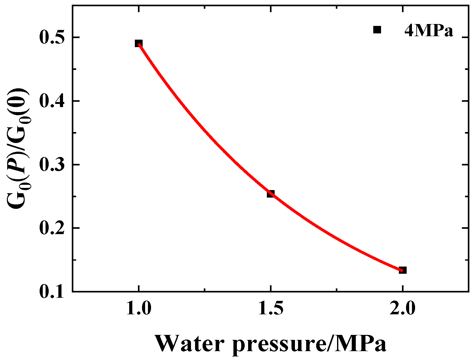
As shown in Figure 11, which was fitted using the data from

Table 11. Value of instantaneous elastic shear modulus under different water pressures.

$\mathbf{Viscoelastic} \mathbf{Shear} \mathbf{Modulus}/\mathbf{GPa}$	Water Pressure/MPa	Effective Shear Stress/MPa
		4	5	6	7	8
$G_0(0)$	0	15.688	19.61	23.532	27.454	31.376
$G_0(p)$	1	7.692	9.615	11.538	13.461	15.384
	1.5	3.98	4.975	5.97	6.965	7.96
	2	2.1	2.625	3.15	3.675	4.2
$G_0(p)/G_0(0)$	1	0.490
	1.5	0.254
	2	0.134

, the following relationship can be obtained:

$${\displaystyle \frac{G_0(P)}{G_0(0)}}=a\times b^P$$

(34)

where $G_0(P)$ is the instantaneous elastic shear modulus under any water pressure, $G_0(0)$ is the instantaneous elastic shear modulus under no water pressure, $P$ is the water pressure, and $a,b$ is the fitting parameter. The fitting coefficient and fitting degree statistics of the viscoelastic shear modulus and water pressure are shown in

Table 12. Fitting coefficient between viscoelastic shear modulus with water pressure.

Effective Shear Stress	a	b	Degree of Fitting	F	p
4~8 MPa	1.810	0.270	0.999	999	<0.05

. According to the fitting results, this functional relationship can well represent the change of the law of instantaneous elastic shear modulus with water pressure. Performing an F-test on the fitting results, a p-value of less than 0.05 indicates that the fitting is statistically significant.

The seepage damage variable of the viscoelastic shear modulus can be expressed as:

$$D_P=\left\{\begin{array}{l}0,\hspace{0.33em}\hspace{0.33em}\hspace{0.33em}\hspace{0.33em}\hspace{0.33em}\hspace{0.33em}\hspace{0.33em}\hspace{0.33em}\hspace{0.33em}\hspace{0.33em}\hspace{0.33em}\hspace{0.33em}\hspace{0.33em}\hspace{0.33em}\hspace{0.33em}\hspace{0.33em}\hspace{0.33em}\hspace{0.33em}\hspace{0.33em}\hspace{0.33em}\hspace{0.33em}\hspace{0.33em}\hspace{0.33em}\hspace{0.33em}\hspace{0.17em}\hspace{0.17em}P=0\\ 1-G_1(P)/G_1(0),\hspace{0.33em}\hspace{0.33em}\hspace{0.33em}\hspace{0.33em}\hspace{0.33em}\hspace{0.33em}\hspace{0.33em}\hspace{0.33em}\hspace{0.33em}\hspace{0.33em}\hspace{0.33em}\hspace{0.33em}P>0\end{array}\right.$$

(35)

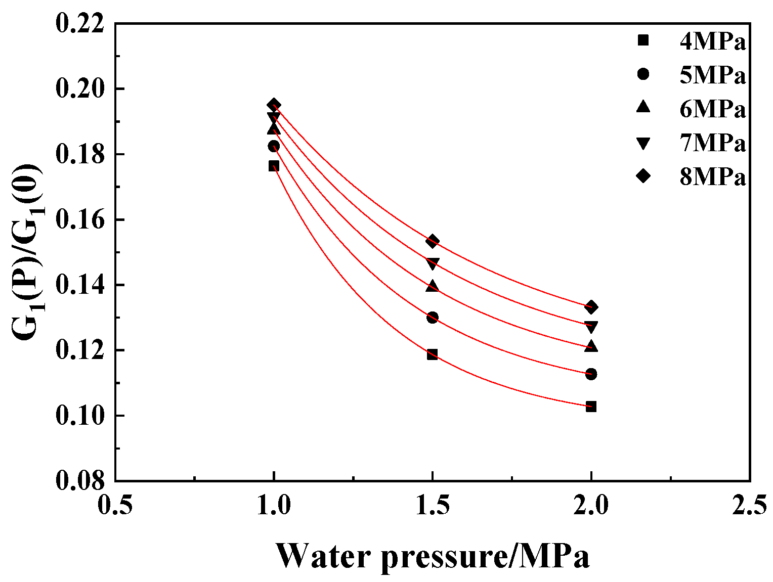
As shown in Figure 12, which was fitted using the data from

Table 13. Value of viscoelastic shear modulus under different water pressures.

$\mathbf{Viscoelastic} \mathbf{Shear} \mathbf{Modulus}/\mathbf{GPa}$	Water Pressure/MPa	Effective Shear Stress/MPa
		4	5	6	7	8
$G_1(0)$	0	1.508	1.677	1.846	2.015	2.184
$G_1(p)$	1	0.266	0.306	0.346	0.386	0.426
	1.5	0.179	0.218	0.257	0.296	0.335
	2	0.155	0.189	0.223	0.257	0.291
$G_1(p)/G_1(0)$	1	0.176	0.182	0.187	0.192	0.195
	1.5	0.119	0.130	0.139	0.147	0.153
	2	0.103	0.113	0.121	0.128	0.133

, the following relationship can be obtained:

$${\displaystyle \frac{G_1(P)}{G_1(0)}}=a-b\times c^P$$

(36)

where $G_1(P)$ is the viscoelastic shear modulus under any water pressure, $G_1(0)$ is the viscoelastic shear modulus under no water pressure, $P$ is the water pressure, and $a,b,c$ is the fitting parameter. The fitting coefficient and fitting degree statistics of viscoelastic shear modulus and water pressure are shown in

Table 14. Fitting coefficient between viscoelastic shear modulus with water pressure.

Effective Shear Stress	4 MPa	5 MPa	6 MPa	7 MPa	8 MPa
a	0.097	0.104	0.109	0.113	0.115
b	−1.050	−0.721	−0.535	−0.420	−0.345
c	0.076	0.109	0.146	0.188	0.234
Degree of fitting	0.999	0.999	0.999	0.999	0.999
F	999
p	<0.05

. According to the fitting results, this functional relationship can well represent the change of the law of viscoelastic shear modulus with water pressure. Performing an F-test on the fitting results, a p-value of less than 0.05 indicates that the fitting is statistically significant.

The seepage damage variable of the viscoelastic viscosity coefficient can be expressed as:

$$D_P=\left\{\begin{array}{l}0,\hspace{0.33em}\hspace{0.33em}\hspace{0.33em}\hspace{0.33em}\hspace{0.33em}\hspace{0.33em}\hspace{0.33em}\hspace{0.33em}\hspace{0.33em}\hspace{0.33em}\hspace{0.33em}\hspace{0.33em}\hspace{0.33em}\hspace{0.33em}\hspace{0.33em}\hspace{0.33em}\hspace{0.33em}\hspace{0.33em}\hspace{0.33em}\hspace{0.33em}\hspace{0.33em}\hspace{0.33em}\hspace{0.33em}\hspace{0.33em}\hspace{0.17em}\hspace{0.17em}P=0\\ 1-{\eta }_1(P)/{\eta }_1(0),\hspace{0.33em}\hspace{0.33em}\hspace{0.33em}\hspace{0.33em}\hspace{0.33em}\hspace{0.33em}\hspace{0.33em}\hspace{0.33em}\hspace{0.33em}\hspace{0.33em}\hspace{0.33em}\hspace{0.33em}\hspace{0.33em}P>0\end{array}\right.$$

(37)

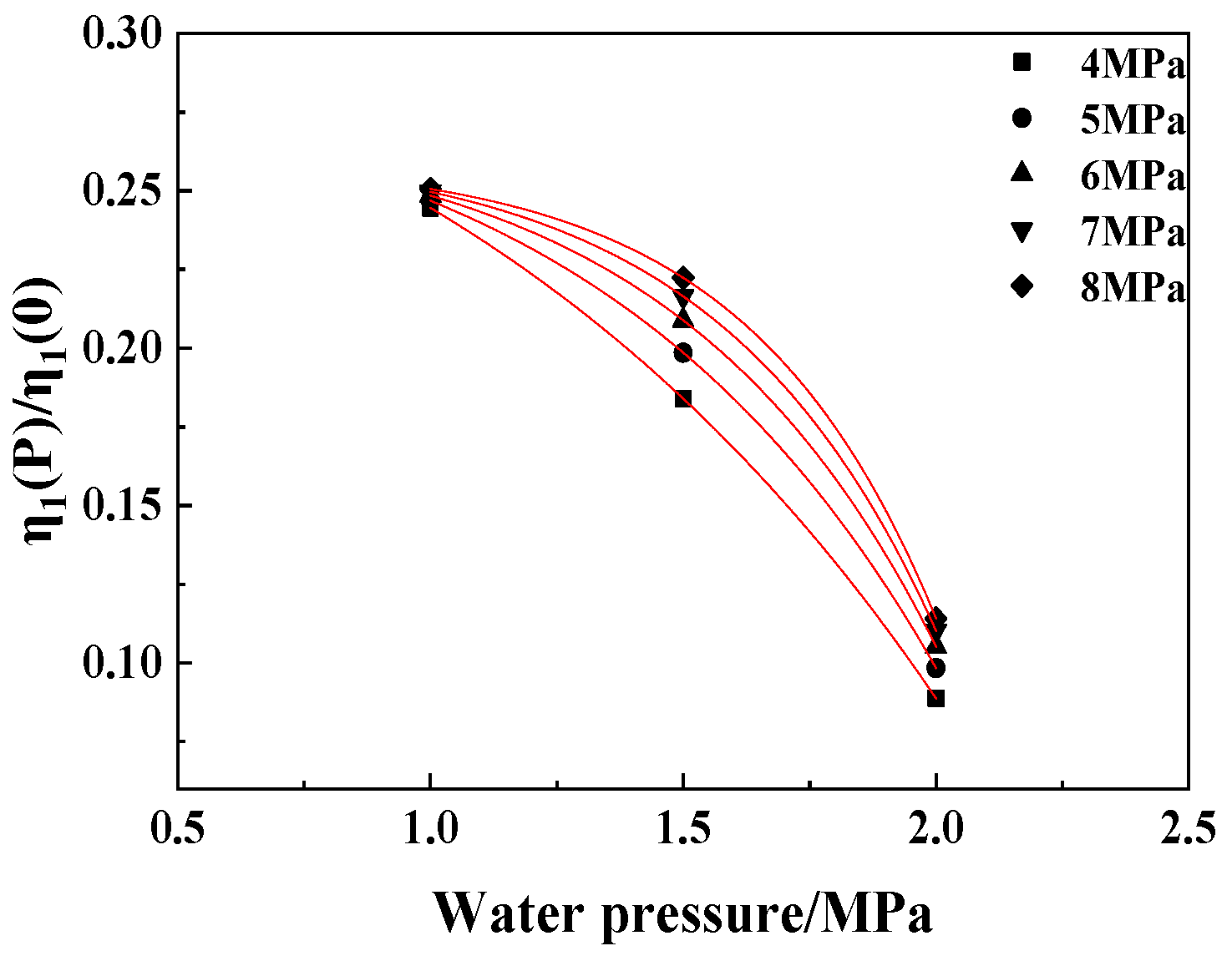
As shown in Figure 13, which was fitted using the data from

Table 15. Value of viscoelastic viscosity coefficient under different water pressure.

$\mathbf{Viscoelastic} \mathbf{Viscous} \mathbf{Coefficient}/\mathbf{GPa}·\mathbf{h}$	Water Pressure/MPa	Effective Shear Stress/MPa
		4	5	6	7	8
${\eta }_1(0)$	0	0.0462	0.0559	0.0656	0.0753	0.0850
${\eta }_1(p)$	1	0.0113	0.0138	0.0163	0.0188	0.0213
	1.5	0.0085	0.0111	0.0137	0.0163	0.0189
	2	0.0041	0.0055	0.0069	0.0083	0.0097
${\eta }_1(p)/{\eta }_1(0)$	1	0.245	0.247	0.248	0.250	0.251
	1.5	0.184	0.199	0.209	0.216	0.222
	2	0.089	0.098	0.105	0.110	0.114

, the following relationship can be obtained:

$${\displaystyle \frac{{\eta }_1(P)}{{\eta }_1(0)}}=a+b\times e^{-P/c}$$

(38)

where ${\eta }_1(P)$ is the viscoelastic viscosity coefficient under any water pressure, ${\eta }_1(0)$ is the viscoelastic viscosity coefficient under no water pressure, $P$ is the water pressure, and $a,b,c$ is the fitting parameter. The fitting coefficient and fitting degree statistics of the viscoelastic viscosity coefficient and water pressure are shown in

Table 16. Fitting coefficient between viscoelastic viscosity coefficient and water pressure.

Effective Shear Stress	4 MPa	5 MPa	6 MPa	7 MPa	8 MPa
a	0.351	0.292	0.273	0.265	0.261
b	−0.043	−0.011	−0.004	−0.001	−0.001
c	−1.106	−0.685	−0.520	−0.430	−0.372
Degree of fitting	0.999	0.999	0.999	0.999	0.999
F	999
p	<0.05

. According to the fitting results, this functional relationship can well represent the change in viscoelastic viscosity coefficient with water pressure. Performing an F-test on the fitting results, a p-value of less than 0.05 indicates that the fitting is statistically significant.

According to the data calculated from Table 11, Table 13 and Table 15, when the water pressure changes from 0 MPa to 2 MPa, the relative change rates of the instantaneous elastic shear modulus, viscoelastic shear modulus, and viscoelastic viscosity coefficient are 86.6%, 89.7%, and 91.1%, respectively. Therefore, it can be roughly concluded that the viscoelastic viscosity coefficient is more significantly affected by the change in water pressure and is more sensitive to the variation in water pressure.

3.4. Time-Dependent Hydro-Mechanical Coupling Shear Creep Model with Damaged Body

According to the above model analysis, before the applied effective shear load does not reach the long-term shear strength of the joint surface, the steady material parameters in the traditional Nishihara linear model are transformed into time-dependent parameters related to time, effective shear stress, and osmotic water pressure. The initial values of the creep parameters are determined by the relationship between the initial values of each creep parameter and the effective shear stress. Then, the parameters have a certain change law with time, and the deterioration effect of seepage on the parameters is taken into account by the seepage damage variable, so as to complete the revision of the creep model during the initial creep and stable creep stages. Then, the joint surface reaches the long-term shear strength and shear failure occurs, that is, the joint surface enters the accelerated creep stage. At this stage, a damaged body is introduced. When the damaged body is started, the damage degree will be aggravated with the increase in creep time and water pressure. Based on the above, stress–seepage coupling with a shear creep constitutive model of joint surface is established, which reflects the characteristics of rock creep at each stage:

$$\gamma (t)=\left\{\begin{array}{l}\left[{\displaystyle \frac{1}{G_0(\tilde{\tau },p)}}+{\displaystyle \frac{1}{G_1(\tilde{\tau },p,t)}}(1-e^{{\displaystyle \frac{-G_1(\tilde{\tau },p,t)}{{\eta }_1(\tilde{\tau },p,t)}}t})\right]\tilde{\tau },\hspace{0.33em}\hspace{0.33em}\hspace{0.33em}\hspace{0.33em}\hspace{0.33em}\hspace{0.33em}\hspace{0.33em}\hspace{0.33em}\hspace{0.33em}\hspace{0.33em}\tilde{\tau }<{\tau }_s\\ \left[{\displaystyle \frac{1}{G_0}}+{\displaystyle \frac{1}{G_1}}(1-e^{{\displaystyle \frac{-G_1}{{\eta }_1}}t})\right]\tilde{\tau }+{\displaystyle \frac{\tilde{\tau }}{E_0}}{(1-{\displaystyle \frac{t}{t_D}})}^{-\alpha P},\hspace{0.33em}\hspace{0.33em}\hspace{0.33em}\hspace{0.33em}\hspace{0.33em}\hspace{0.33em}\hspace{0.33em}\hspace{0.33em}\hspace{0.33em}\hspace{0.33em}\hspace{0.33em}\tilde{\tau }\ge {\tau }_s\end{array}\right.$$

(39)

where $G_0(\tilde{\tau })$ is the instantaneous elastic shear modulus related to the effective shear stress, $G_1(\tilde{\tau },p,t)$ is the viscoelastic shear modulus at any time related to the effective shear stress and water pressure and time, and its initial value $G_1(\tilde{\tau },p,t_0)$ is related to the effective shear stress and the seepage damage variable. ${\eta }_1(\tilde{\tau },p,t)$ is the viscoelastic viscosity coefficient at any time related to the effective shear stress, water pressure, and time, and its initial value ${\eta }_1(\tilde{\tau },p,t_0)$ is related to the effective shear stress and the seepage damage variable. The relationships are as follows:

$$G_0(\tilde{\tau },p)=a\times \tilde{\tau }(1-D_P)$$

(40)

$$\begin{array}{l}{G}_1(\tilde{\tau },p,t)=G_1(\tilde{\tau },p,t_0)\left[{\displaystyle \frac{a}{t}}+b\right]\\ G_1(\tilde{\tau },p,t_0)=(a+b\tilde{\tau })(1-D_P)\end{array}$$

(41)

$$\begin{array}{l}{\eta }_1(\tilde{\tau },p,t)={\eta }_1(\tilde{\tau },p,t_0)\left(a+bt\right)\\ {\eta }_1(\tilde{\tau },p,t_0)=(a+b\tilde{\tau })(1-D_P)\end{array}$$

(42)

In conclusion, the constitutive model reflects not only the viscoelastic characteristics of the rock joint surface at the initial creep stage and the stable creep stage, but also the viscoplastic characteristics of the joint surface at the accelerated creep stage. The relationship and change trend of the parameters and time of the initial and stable creep stages and effective shear stress were studied. The seepage damage variable was introduced to describe the deterioration effect of seepage on creep parameters and the change rule. When the effective shear stress was greater than the long-term shear strength of the joint surface, the plastic damage variable was activated to ensure the creep acceleration stage. The influence of seepage on the creep is considered in the whole creep process. At the same time, a set of shear creep models of a regular sawtooth joint under the coupling of stress and seepage is established by considering the effect of water pressure, fluctuation height and normal stress on the joint surface.

4. The Verification of the Shear Creep Model

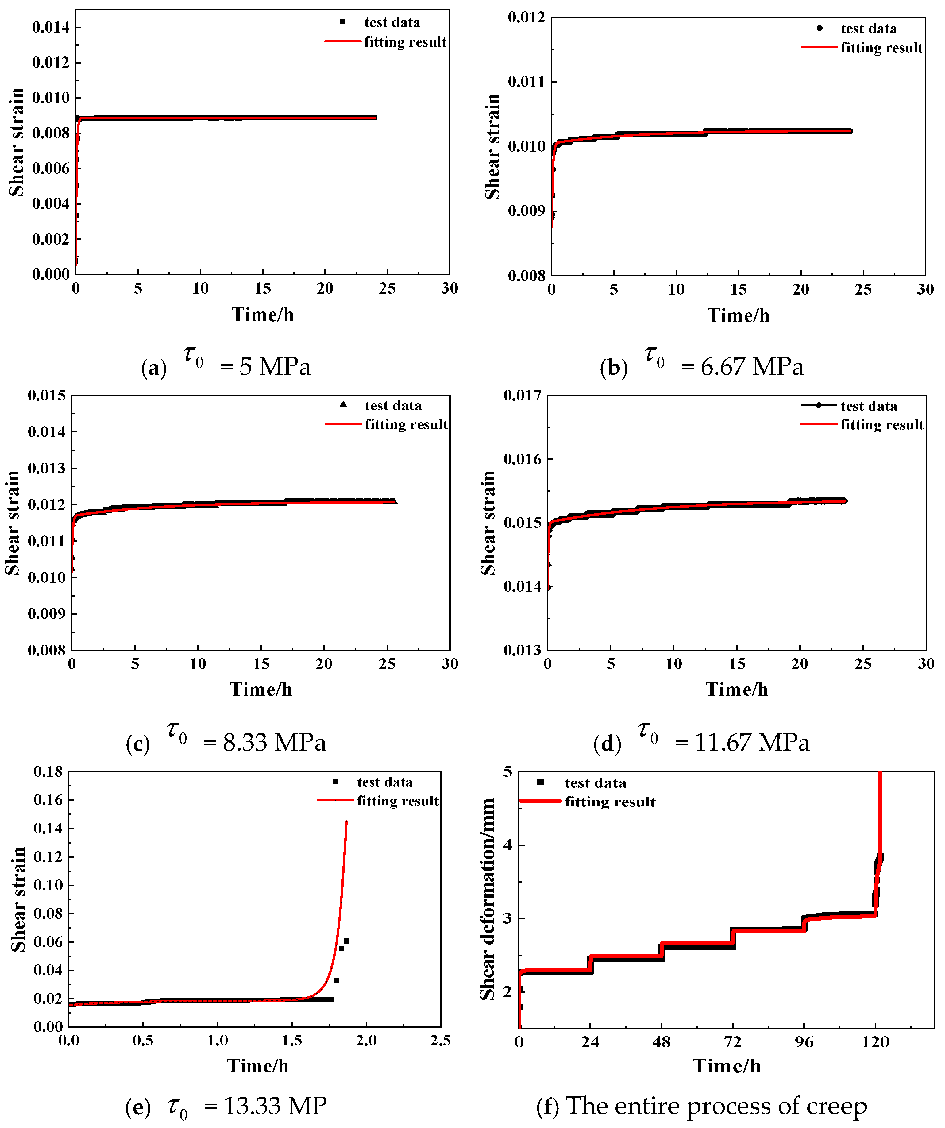
To verify the validity of the shear creep model under the coupling of stress and seepage, the model is used to fit the shear creep curves of other granite joint surfaces to judge the applicability of the model. Because the samples are taken from the same rocks in the same area, it is believed that the creep parameters of the samples conform to the same change law. The verification sample contains a joint surface with a fluctuation height of 10 mm, applied normal stress of 5 MPa, and applied water pressure of 1 MPa.

Table 17. Creep parameters of the sample under the action of effective shear stress at all levels.

Effective Shear Stress/MPa	Time/h	${\mathbf{G}}_0$$/\mathbf{GPa}$	${\mathit{G}}_1$$/GPa$	${\mathit{\eta }}_1$$/GPa·h$
1.22	0.5	3.750	0.151	0.012
	4	3.750	0.150	0.016
	8	3.750	0.150	0.034
	12	3.750	0.150	0.051
	16	3.750	0.150	0.068
	20	3.750	0.150	0.087
	24	3.750	0.150	0.106
2.89	0.5	8.888	0.325	0.025
	4	8.888	0.322	0.035
	8	8.888	0.322	0.072
	12	8.888	0.321	0.109
	16	8.888	0.321	0.147
	20	8.888	0.321	0.185
	24	8.888	0.321	0.227
4.55	0.5	13.996	0.468	0.035
	4	13.996	0.466	0.051
	8	13.996	0.465	0.105
	12	13.996	0.465	0.159
	16	13.996	0.464	0.213
	20	13.996	0.464	0.269
	24	13.996	0.464	0.322
6.22	0.5	19.134	0.576	0.042
	4	19.134	0.570	0.062
	8	19.134	0.569	0.128
	12	19.134	0.569	0.195
	16	19.134	0.568	0.261
	20	19.134	0.563	0.325
	24	19.134	0.563	0.388
7.89	0.5	24.273	0.680	0.050
	4	24.273	0.671	0.074
	8	24.273	0.666	0.150
	12	24.273	0.664	0.227
	16	24.273	0.661	0.303
	20	24.273	0.652	0.377
	24	24.273	0.652	0.453

shows the creep parameters of the sample under various effective shear stresses.

Figure 14 shows the comparison between the fitted value and the actual test value under single-stage shear load and the entire creep process. The fitting results under single-stage shear load have higher consistency due to the finer fitting parameters, and the fitting data in the entire creep process are slightly different from the test data due to the complexity of parameter relationships. However, the results still show a high consistency, and the basic characteristics of the whole creep process of the sample are fitted, which indicates that the shear creep model has a certain rationality and effectiveness.

5. Research Limitations

Although the shear creep constitutive model established in this paper can reflect the creep characteristics of rock joint surfaces under stress–seepage coupling, it still has the following limitations. First, a global sensitivity analysis of the model parameters has not been conducted, making it difficult to quantitatively evaluate the relative contributions of each parameter to the creep response and their order of dominance. Second, the current study only considers the indirect coupling of the stress field, the seepage field, and time, whereas the interactions among multiple fields in actual engineering environments may significantly alter the long-term deformation behavior of the joint surface. Third, the model validation process lacks systematic and rigorous statistical testing, so the reliability of the extrapolation and generalization capability of the model has not been fully quantified. To address these limitations, we will focus on the following improvements in our future work: carrying out parameter screening and simplification based on sensitivity analysis using methods proposed by researchers [41,42,43,44,45]; establishing both a fully coupled multi-field model that accounts for stress, seepage, and time and a predictive model for the time to shear creep failure; and introducing systematic statistical testing methods to rigorously evaluate the accuracy and robustness of the model.

To further enhance the value of this model for engineering design and construction guidance, future efforts can expand and improve the constitutive model in the following directions. First, consider the degradation and wear effects of joint surface roughness and establish dynamically updated evolution equations for joint morphology, so that the model can more realistically reflect the geometric deterioration during long-term shearing. Second, introduce cyclic or variable-amplitude loading to study the creep accumulation law under non-steady stress conditions, thereby making the model applicable to dynamic engineering scenarios such as earthquakes, blasting, and construction disturbances [46,47]. Third, incorporate time–space scale effects into the model and combine laboratory test data with field monitoring data to establish a scaled constitutive relationship that can be extrapolated to the engineering scale. Through continuous improvement in these directions, the model is expected to more comprehensively describe the complex creep behavior of rock joint surfaces under multi-field and multi-factor coupling, thus providing a more reliable theoretical basis for engineering design parameter selection, long-term deformation prediction, and construction risk control.

6. Conclusions

This paper mainly studies the shear creep model under the coupling of stress and seepage. The main conclusions are summarized as follows:

(1) The calculation method of the effective shear stress in the stress–seepage coupled shear creep test is determined and the relationship between the effective shear stress and the normal stress applied on the joints, the fluctuation height of the joints, and the water pressure is established.

(2) An improved rock creep constitutive model is established by transforming the steady material parameters in the linear model into time-dependent parameters related to factors such as time, effective shear stress, and osmotic water pressure and by introducing damage variables into the combined linear model on the basis of damage fracture mechanics to characterize the nonlinear deformation at the accelerated creep stage.

(3) A damaged body is introduced to simulate the deformation within the accelerated creep stage. When the damaged body is started, the plastic damage of the rock material begins to appear and gradually accumulates. The damage degree increases with the increase in creep time, and the damaged body also reflects that the damage intensifies with an increase in water pressure. The plastic damaged body describes the nonlinear accelerated deformation characteristics of the rock material when it enters the accelerated creep stage.

This proposed constitutive model not only reflects the viscoelastic characteristics of the rock joint surface during the primary and steady-state creep stages but also captures its viscoplastic characteristics during the accelerated creep stage, accounting for the influence of seepage throughout the entire creep process. This provides theoretical support for engineering design and construction.

References

1. Hu, B.; Jiang, H.F.; Hu, X.L.; Guo, L.N.; Wang, X.G. Analysis of shear rheological mechanical properties of fuchsia mudstone. Chin. J. Rock Mech. Eng. 2012, 31, 1242−1246. [Google Scholar]
2. Xu, W.Y.; Yang, S.Q. Experiment and modeling and investigating on shear rheological property of joint rock. Chin. J. Rock Mech. Eng. 2005, 24, 5536–5542. [Google Scholar]
3. Xu, T.; Xu, Q.; Tang, C.A.; Ranjith, P.G. The evolution of rock failure with discontinuities due to shear creep. Acta Geotech. 2013, 8, 567–581. [Google Scholar] [CrossRef]
4. Wang, J.A.; Wang, Y.X.; Cao, Q.J.; Ju, Y.; Mao, L.T. Behavior of microcontacts in rock joints under direct shear creep loading. Int. J. Rock Mech. Min. Sci. 2015, 78, 217–229. [Google Scholar] [CrossRef]
5. Sheng, M.R.; Zhang, Q.Z. Study of shear creep characteristics of greenschist discontinuities. Chin. J. Rock Mech. Eng. 2010, 29, 1149–1155. [Google Scholar]
6. Yang, S.Q.; Xu, W.Y.; Yang, Q.L. Investigation on shear rheological mechanical properties of shale in Longtan Hydropower Project. Rock Soil Mech. 2007, 28, 895–902. [Google Scholar]
7. Liu, X.Z.; Su, J.W.; Wang, X.X. Experiment investigation on shear rheological properties of tuff lava with different grades. Chin. J. Rock Mech. Eng. 2009, 28, 190–197. [Google Scholar]
8. Wu, G.J.; Chen, W.Z.; Jia, S.P.; Yang, J.P. Shear creep experiments for anchorage interface mechanics and nonlinear rheological model of rocks. Chin. J. Rock Mech. Eng. 2010, 29, 520–527. [Google Scholar]
9. Zhu, M.L.; Zhu, Z.D.; Li, Z.J.; Chen, W.Z.; Zhu, J.B. Preliminary study of non-stationary shear rheological model of wall of long, large and deep-buried tunnel. Chin. J. Rock Mech. Eng. 2008, 7, 1436–1441. [Google Scholar]
10. Nazary Moghadam, S.; Mirzabozorg, H.; Noorzad, A. Modeling time-dependent behavior of gas caverns in rock salt considering creep, dilatancy and failure. Tunn. Undergr. Space Technol. 2013, 33, 171–185. [Google Scholar] [CrossRef]
11. Drescher, K.; Handley, M.F. Aspects of time-dependent deformation in hard rock at great depth. J. S. Afr. Inst. Min. Metall. 2003, 103, 325–335. [Google Scholar]
12. Asanov, V.A.; Pan’kov, I.L. Deformation of salt rock joints in time. J. Min. Sci. 2004, 40, 355–359. [Google Scholar] [CrossRef]
13. Yang, S.Q.; Cheng, L. Non-stationary and nonlinear visco-elastic shear creep model for shale. Int. J. Rock Mech. Min. Sci. 2011, 48, 1011–1020. [Google Scholar] [CrossRef]
14. Chen, G.Q.; Jian, D.H.; Chen, Y.H.; Wan, Y.; Lin, Z.H. Shear creep characteristics of red sandstone after freeze-thaw with different water contents. Chin. J. Rock Mech. Eng. 2021, 43, 661–669. [Google Scholar]
15. Zhu, H.H.; Ye, B. Experiment study on mechanical properties of rock creep in saturation. Chin. J. Rock Mech. Eng. 2002, 21, 1791–1796. [Google Scholar]
16. Wang, D.S.; Song, Y.J. Present state of research and its development trend on rock rheological mechanics. Sichuan Build. Sci. 2015, 41, 61–65. [Google Scholar]
17. Xu, H.; Hu, B.; Tang, H.M.; Chen, J.L. Experiment and model research on shear rheological properties of saturated sandstone. Chin. J. Rock Mech. Eng. 2010, 29, 2775–2781. [Google Scholar]
18. Yu, Y.J.; Zhang, W.; Zhang, G.N.; Jiang, T.F.; Zhang, C.H. Study of nonlinear shear creep model and creep property experiment of water-rich soft rock. J. Chin. Coal Soci. 2018, 43, 1780–1788. [Google Scholar]
19. Lai, Y.C.; Li, P.W.; Deng, H.; Liu, D.; Su, H. Study on shear creep behavior of mudstone under saturated-dehydrated cycling. Water Res. Hydropower Eng. 2019, 50, 195–201. [Google Scholar]
20. Han, S.L.; Chen, T.L. Shear creep characteristics and constitutive model of saturated and degraded dam foundation rock with weak interlayer. China Meas. Test 2021, 47, 41–46+132. [Google Scholar]
21. Hu, B.; Huang, L.H.; Ding, J.; Li, J.; Cui, K. Study on shear creep test and constitutive model of soft rock under repeated water/air pressure cycle. Nonferrous Met. 2022, 74, 106–115. [Google Scholar]
22. Wu, L.Z.; Li, B.; Huang, R.Q.; Sun, P. Experimental study and modeling of shear rheology in sandstone with non-persistent joints. Eng. Geol. 2017, 222, 201–211. [Google Scholar] [CrossRef]
23. Xu, M.; Jin, D.; Song, E. A rheological model to simulate the shear creep behavior of rockfills considering the influence of stress states. Acta Geotech. 2018, 13, 1313–1327. [Google Scholar] [CrossRef]
24. Wang, J.D.; Wang, X.G.; Zhan, H.B.; Qiu, H.J.; Hu, S. A new superlinear viscoplastic shear model for accelerated rheological deformation. Comput. Geotech. 2019, 114, 103132. [Google Scholar] [CrossRef]
25. Lin, H.; Zhang, X.; Cao, R.H.; Wen, Z.J. Improved nonlinear Burgers shear creep model based on the time-dependent shear strength for rock. Environ. Earth Sci. 2020, 79, 149–157. [Google Scholar] [CrossRef]
26. Tang, H.; Wang, D.P.; Huang, R.Q.; Pei, X.J.; Chen, W.L. A new rock creep model based on variable-order fractional derivatives and continuum damage mechanics. Bull. Eng. Geol. Environ. 2017, 77, 375–383. [Google Scholar] [CrossRef]
27. Ping, C.; Wen, Y.D.; Wang, Y.X.; Yuan, H.P.; Yuan, B.X. Study on nonlinear damage creep constitutive model for high-stress soft rock. Environ. Earth Sci. 2016, 75, 900. [Google Scholar] [CrossRef]
28. Zhou, H.W.; Wang, C.P.; Han, B.B.; Duan, Z.Q. A creep constitutive model for salt rock based on fractional derivatives. Int. J. Rock Mech. Min. Sci. 2011, 48, 116–121. [Google Scholar] [CrossRef]
29. Wang, J.G.; Jin, Q.; Liang, B.; Liu, W.F. Creep features and the creep model of the soft rock variable parameters under the impact of the seepage pressure in the creep process. J. Saf. Environ. 2016, 16, 120–125. [Google Scholar]
30. Liu, C.M.; Zhang, H. Research on Creep Model of Roadway Surrounding Rock Based on Variable Creep Parameters. Saf. Coal Mines 2020, 51, 39–43+49. [Google Scholar]
31. Pan, X.M.; Yang, Z.; Xu, J.C. Application study of nonstationary Nishihara viscoelasto-plastic rheological model. Chin. J. Rock Mech. Eng. 2011, 30, 2640–2646. [Google Scholar]
32. Zhang, F.R.; Jiang, A.N.; Yang, X.R. Effect of pore water pressure on shear creep characteristics of serrate structural plane. Rock Soil Mech. 2020, 41, 2901–2912. [Google Scholar]
33. Zhang, F.R.; Jiang, A.N.; Yang, X.R. Experimental and model research on shear creep of granite under freeze-thaw cycles. Rock Soil Mech. 2020, 41, 509–519. [Google Scholar]
34. Yang, K.; Han, C.; Liu, X.L. Creep experiments and theoretical model on sandstone under step loading and unloading. J. Yangtze River Sci. Res. Inst. 2021, 38, 97–102+109. [Google Scholar]
35. Zhang, L.L.; Chen, H.; Yao, Z.S.; Wang, X.J. Prediction model for rock creep failure time under conventional triaxial compression. Rock Soil Mech. 2025, 46, 2011–2022. [Google Scholar]
36. Liu, K.Y.; Xue, Y.T.; Zhou, H. Study on 3D nonlinear visco-elastic -plastic creep constitutive model with parameter unsteady of soft rock based on improved Bingham model. Rock Soil Mech. 2018, 39, 4157–4164. [Google Scholar]
37. Wang, Y.; Lu, X.Y.; Zhai, G.L. Non-Stationary Creep Model for Rock Based on Nishihara Model. Sci. Tech. Eng. 2022, 22, 676–682. [Google Scholar]
38. Sui, Q.; Chen, W.Z.; Wang, L.Y.; Li, H. Investigation on hydro-mechanical coupling shear creep properties of jointed rock masses. Tunn. Undergr. Space Technol. 2025, 165, 106880. [Google Scholar] [CrossRef]
39. Yan, Y. Research on Rock Creep Tests Under Seepage Flow and Variable Parameters Creep Equation. Ph.D. Thesis, Tsinghua University, Beijing, China, 2009. [Google Scholar]
40. Li, Q.Q. Curve fitting method for creep parameter of soft rock. Chin. J. Rock Mech. Eng. 1998, 5, 81–86. [Google Scholar]
41. Vu-Bac, N.; Lahmer, T.; Zhuang, X.; Nguyen-Thoi, T.; Rabczuk, T. A software framework for probabilistic sensitivity analysis for computationally expensive models. Adv. Eng. Softw. 2016, 100, 19–31. [Google Scholar] [CrossRef]
42. Vu-Bac, N.; Nguyen, A.H.; Luong, V.H. Uncertainty analysis of static fatigue of Hi-Nicalon bundles. Eng. Anal. Bound. Elem. 2024, 167, 105862. [Google Scholar] [CrossRef]
43. Nguyen, T.C.; Vu-Bac, N.; Budarapu, P.R. A Kriging-based uncertainty quantification for fracture assessment. Int. J. Comput. Methods 2025, 22, 2450045. [Google Scholar] [CrossRef]
44. Vu-Bac, N.; Le-Anh, T.; Rabczuk, T. A Machine Learning based uncertainty quantification for compressive strength of high-performance concrete. Front. Struct. Civ. Eng. 2025, 19, 824–836. [Google Scholar] [CrossRef]
45. Nguyen, T.C.; Vu-Bac, N. Machine Learning-Assisted Sensitivity Analysis for Stochastic Fatigue Life Modeling of Metals. Int. J. Mech. Syst. Dyn. 2025, 5, 481–494. [Google Scholar] [CrossRef]
46. Cai, C.; Li, J.; Zhai, C.; Wang, B.; Xue, J.; Dong, Z.; Zhu, Z. Crack propagation characteristics in shale under cyclic in situ methane detonation impact fracturing. Energy Fuel 2026, 40, 6064–6082. [Google Scholar] [CrossRef]
47. Xue, Y.; Wang, L.C.; Liu, Y.; Ranjith, P.G.; Cao, Z.Z.; Shi, X.Y.; Gao, F.; Kong, H.L. Brittleness evaluation of gas-bearing coal based on statistical damage constitution model and energy evolution mechanism. J. Cent. South Univ. 2025, 32, 566–581. [Google Scholar] [CrossRef]
Figure 1. Hydro-mechanical coupling shear creep model.
Symmetry 18 00850 g001
Figure 2. Regular serration of joint surface.
Symmetry 18 00850 g002
Figure 3. Shear creep curves under hydro-mechanical coupling of joint surface with different water pressures: (a) 1 MPa, (b) 1.5 MPa, (c) 2 MPa, and (d) Comparison.
Symmetry 18 00850 g003
Figure 4. Variation curve of viscoelastic shear modulus with time.
Symmetry 18 00850 g004
Figure 5. Fitting curve of t × G 1 ( t ) / G 1 ( t 0 ) and t .
Symmetry 18 00850 g005
Figure 6. Variation curve of viscoelastic viscosity coefficient with time.
Symmetry 18 00850 g006
Figure 7. Fitting curve of η 1 ( t ) / η 1 ( t 0 ) and t .
Symmetry 18 00850 g007
Figure 8. Variation curve of elastic shear modulus with time.
Symmetry 18 00850 g008
Figure 9. Variation curve of initial viscoelastic shear modulus with effective shear stress.
Symmetry 18 00850 g009
Figure 10. Variation curve of initial viscoelastic viscosity coefficient with effective shear stress.
Symmetry 18 00850 g010
Figure 11. Variation curve of G 0 ( p ) / G 0 ( 0 ) with water pressure.
Symmetry 18 00850 g011
Figure 12. Variation curve of G 1 ( p ) / G 1 ( 0 ) with water pressure.
Symmetry 18 00850 g012
Figure 13. Variation curve of η 1 ( p ) / η 1 ( 0 ) with water pressure.
Symmetry 18 00850 g013
Figure 14. Fitting of shear creep curve of joint surface with undulating height of 10 mm and normal pressure of 5 MPa.
Symmetry 18 00850 g014