Sustainable Cryptography: Carbon Asymmetry in Partially Homomorphic Encryption in the Cloud

Abstract

Encryption protects data in the cloud but adds energy cost, especially for partially homomorphic encryption (PHE) schemes that allow computation on encrypted data. Their carbon footprint across cloud data center deployments remains underexplored. We benchmark eight PHE algorithms from the LightPHE open-source Python library, including RSA, ElGamal, Exponential ElGamal, Paillier, Damgård–Jurik, Okamoto–Uchiyama, Goldwasser–Micali, and Elliptic Curve ElGamal, across six cloud environments, and use timing data as input to a carbon estimation model covering Scope 1, Scope 2, and Scope 3 emissions across ten data center configurations. We ground the energy model with a dedicated Intel RAPL calibration on bare-metal hardware using 30 repetitions per configuration. The calibration measures average CPU package power at 34.7 W and total system power at 48.4 W, showing that a fixed 150 W CPU-only assumption overestimates actual CPU power by a factor of 4.3. We present calibrated estimates alongside a 150 W server-class scenario and a sensitivity analysis across power, PUE, and grid carbon intensity. Elliptic curve schemes provide equivalent classical security at a fraction of the energy cost of RSA, and algorithm-specific mathematical structure drives order-of-magnitude differences in carbon output. These results reveal an asymmetry between security and carbon cost across PHE algorithms and establish a sustainable-cryptography baseline for future PQC-based homomorphic schemes.

1. Introduction

The advent of quantum computing poses a growing threat to existing cryptographic systems. Recent developments, such as Google’s Willow quantum chip and Microsoft’s Majorana 1 chip, have shown progress in quantum error correction, potentially bringing us closer to cryptographically relevant quantum computers (CRQCs) [1,2,3]. In response, the National Institute of Standards and Technology (NIST) finalized the first three post-quantum cryptography (PQC) standards in 2024, including ML-KEM, ML-DSA, and SPHINCS+, to prepare for long-term security against quantum attacks [4]. These shifts make the choice and implementation of encryption methods more important than ever, especially in cloud environments where both security and resource use must be considered together.

At the same time, data center energy consumption is rising sharply. The International Energy Agency (IEA) estimates that data centers consume roughly 1 percent of global electricity, with projections indicating this could double by 2026 [5]. In the United States, estimates suggest data center demand may rise from 17 GW in 2022 to 35 GW by 2030 [6,7]. As organizations move more operations to the cloud, the environmental cost of computation, including encryption, becomes a practical concern that can no longer be ignored.

Within this data center energy envelope, cryptographic operations occupy a persistent and growing share. Nearly all modern web traffic is now encrypted at the transport layer, and each secure session involves asymmetric cryptographic operations during the handshake and rekeying. Beyond transport-layer encryption, confidential computing deployments and privacy-preserving cloud workloads introduce additional cryptographic overhead that scales with the volume of processed data. Homomorphic encryption sits at the upper end of this cost spectrum, because a single operation can require orders of magnitude more CPU cycles than symmetric encryption, and this cost grows further with key size. When these per-operation costs are multiplied across the scale of modern cloud deployments, cryptographic energy becomes a design-relevant dimension rather than a fixed overhead.

These two pressures are directly connected. Post-quantum algorithms generally require larger keys and heavier computation, so each cryptographic operation draws more energy than its classical counterpart. On the infrastructure side, carbon-aware scheduling has begun to shift workloads toward times and locations where the grid is cleaner [8], and early eco-aware assessments of computing workloads now report energy per operation alongside throughput as a design metric [9]. In cryptography, this kind of environmental accounting is still uncommon. We use the term sustainable cryptography to describe this emerging area where cryptographic design and deployment choices are evaluated together with their energy consumption and carbon costs.

Homomorphic encryption (HE) addresses one side of this problem: it allows computation on encrypted data without decryption, removing the need to transmit private keys to the cloud [10]. Fully homomorphic encryption (FHE) supports both addition and multiplication on ciphertexts but carries a heavy computational burden. Partially homomorphic encryption (PHE), which supports either addition or multiplication, is lighter and more practical for many real-world tasks [11,12]. The PHE schemes evaluated in this study are classical, not post-quantum. We reference PQC developments above only to illustrate the broader trend that stronger cryptography demands more computation and, by extension, more energy. By establishing a measurement methodology and carbon baseline for classical PHE, this work provides a reference point against which the carbon cost of future PQC-based homomorphic schemes, such as those based on lattice problems or nilpotent Lie algebra constructions [13], can be compared.

Researchers have individually examined energy-efficient HE hardware [14,15], lightweight encryption for constrained devices [16], and sustainable data center operation [8]. Yet the connection between the energy profiles of specific PHE algorithms and Scope 1, Scope 2, and Scope 3 emissions across multiple cloud platforms and data center types remains largely unexplored. This work addresses that gap through a scenario-based carbon estimation framework with explicit uncertainty analysis.

In this paper, we developed LightPHE, an open-source Python library that wraps ten established PHE algorithms, including RSA, ElGamal, Paillier, Damgård–Jurik, Okamoto–Uchiyama, Benaloh, Naccache–Stern, Goldwasser–Micali, Exponential ElGamal, and Elliptic Curve ElGamal [17]. The eight algorithms benchmarked in this study were selected on three grounds. First, they represent the main mathematical families of PHE: RSA and ElGamal for multiplicative homomorphism; Paillier, Damgård–Jurik, Okamoto–Uchiyama, and Exponential ElGamal for additive homomorphism under composite or discrete-logarithm groups; Goldwasser–Micali for bitwise XOR; and Elliptic Curve ElGamal for additive operations with small plaintext. Second, all eight support stable key generation across the 80 to 192-bit symmetric-equivalent security range evaluated here. Third, Benaloh and Naccache–Stern were excluded because their key generation fails within practical retry budgets at 2048 bits and above, and Boneh–Goh–Nissim, which is supported by LightPHE but relies on pairing-based arithmetic, was excluded because its computational profile differs from the other schemes and warrants a separate study.

We benchmark LightPHE’s performance across six cloud environments: five Google Colab runtimes, each backed by the same Intel Xeon host CPU but differing in system memory and idle accelerator hardware, and one Microsoft Azure Spark cluster. Since LightPHE is written in pure Python, all cryptographic operations run on the CPU. The accelerators present in some runtimes were never used by our code, so the observed performance differences across these environments reflect variations in CPU allocation and memory subsystems. Beyond time complexity, we introduce a carbon emission estimation model that maps computational workloads to estimated Scope 1, 2, and 3 greenhouse gas emissions across ten data center configurations with varying energy mixes and power usage effectiveness (PUE) values.

A connection to the concept of symmetry runs through this work at two levels. At the algorithmic level, all PHE schemes studied here are asymmetric, meaning encryption and decryption rely on separate keys. This asymmetry is not only a security feature but also a source of computational imbalance: encryption and decryption differ widely in cost, and this imbalance translates directly into unequal energy profiles. At the infrastructure level, the relationship between security strength and environmental cost is itself asymmetric. Increasing key size by a fixed factor can raise energy consumption by orders of magnitude, while switching to a renewable-powered data center can cut emissions by a comparable factor in the opposite direction. Recognizing and quantifying these asymmetries is what allows practitioners to make balanced decisions about where, how, and with which algorithm to encrypt.

Our main contributions are as follows. First, we present a scenario-based carbon estimation framework that connects PHE algorithm performance to Scope 1, 2, and 3 emissions across multiple cloud and data center configurations, an analysis that, to our knowledge, has not been reported for partially homomorphic encryption. Second, we introduce a carbon estimation model that accounts for hardware power draw, PUE, grid carbon intensity, and renewable energy shares, with explicit uncertainty bounds rather than point estimates. Third, we validate the energy model through a dedicated power calibration experiment using Intel RAPL hardware measurements, revealing the gap between assumed and measured CPU power and providing a literature-grounded reference table of power consumption across platform types. Fourth, we present a security-normalized carbon comparison using NIST key size equivalences, showing that elliptic curve schemes achieve equivalent security at roughly 1.6 percent of the carbon cost of RSA-based alternatives. Fifth, we report statistical analysis with 30 repetitions per configuration, revealing that probabilistic key generation algorithms exhibit execution time variability exceeding 400 percent CV, while deterministic elliptic curve operations remain below 5 percent in the calibration experiment.

1.1. Related Work

Several lines of research are relevant to the intersection of homomorphic encryption, energy efficiency, and cloud computing.

On the cryptographic side, fully homomorphic encryption (FHE) allows both addition and multiplication on ciphertexts [18], but at a high computational cost. Partially homomorphic encryption (PHE) restricts operations to either addition or multiplication, offering lower overhead for specific use cases [11,19]. PHE schemes are used in applications like e-voting and Private Information Retrieval, though their scope is limited by the types of operations they support [12,16,19]. Several FHE libraries exist, such as SEAL [20], TenSEAL [21], Pyfhel [22], and PyFHE [23], but dedicated PHE libraries have been lacking until the introduction of LightPHE [17].

Table 1. Scheme-level coverage of major homomorphic encryption libraries. FHE libraries focus on BFV, BGV, and CKKS; classical PHE schemes are supported only by LightPHE.

Library	Focus	Language	Supported Schemes
SEAL [20]	FHE	C++	BFV, CKKS
OpenFHE [24]	FHE	C++	BFV, BGV, CKKS, FHEW, TFHE
HElib [25]	FHE	C++	BGV, CKKS
PALISADE [26]	FHE	C++	BFV, BGV, CKKS
TenSEAL [21]	FHE wrapper	Python over SEAL	BFV, CKKS
Pyfhel [22]	FHE wrapper	Python over SEAL	BFV, CKKS
LightPHE [17]	PHE	Python	RSA, ElGamal, Exp. ElGamal, EC-ElGamal, Paillier, Damgård–Jurik, Okamoto–Uchiyama, Goldwasser–Micali, Benaloh, Naccache–Stern

summarizes the scheme-level coverage of the major homomorphic encryption libraries. SEAL [20], OpenFHE [24], HElib [25], and PALISADE [26] focus on FHE schemes such as BFV, BGV, and CKKS, with no native support for classical PHE. TenSEAL and Pyfhel are Python wrappers for SEAL and inherit the same FHE-only scope. LightPHE is, to the best of our knowledge, the only actively maintained library that provides a unified Python interface to ten classical PHE algorithms. This scheme-level mismatch is why a direct library-to-library runtime comparison is not meaningful at the algorithm level: SEAL does not implement RSA or Paillier, and LightPHE does not implement BFV or CKKS. We use LightPHE in this study because it provides unified coverage of the eight PHE algorithms evaluated here.

On the hardware optimization side, recent work has explored ways to reduce the energy demands of homomorphic encryption. A 2020 IEEE study investigates computing-in-memory (CiM) architectures, showing reduced latency and energy consumption for HE operations [14]. IEEE Spectrum’s 2023 article discusses hardware accelerators like RISE that aim to make HE more practical on edge devices, though data center-level improvements are still needed [15]. These developments point to a way of reducing the energy demands of HE in line with sustainability goals.

On the benchmarking side, a few recent studies have started to measure the practical performance of HE across different platforms. Valera-Rodriguez et al. tested Microsoft SEAL’s FHE implementation on a standard PC and an NVIDIA Jetson Nano edge device, reporting CPU usage and execution time but not energy consumption or emissions [27]. Kupcova et al. carried out a systematic comparison of PHE, somewhat homomorphic, and fully homomorphic schemes, covering Paillier, ElGamal, BFV, and CKKS under identical 128-bit security settings, and measured encryption time, ciphertext expansion, and memory use [28]. These benchmarking efforts are valuable for understanding algorithm-level trade-offs, but none of them connect their performance data to data center energy profiles or carbon emission scopes.

On the environmental assessment side, the energy consumption of data centers has received growing attention. The IEA reports that data centers account for roughly 1 percent of global electricity use, with projections of doubling by 2026 [5]. The EPRI projects that data centers could consume up to 9 percent of US electricity by 2030 [29]. The categorization of Scope 1, Scope 2, and Scope 3 emissions, as defined by the Greenhouse Gas Protocol [30], has become a standard way to measure the environmental footprint of data center operations [31,32]. Yet, to the best of our knowledge, the energy profiles of specific homomorphic encryption algorithms have not been connected to these emission scopes in a single study covering multiple cloud platforms and data center types. Recent work on post-quantum homomorphic schemes, such as the nilpotent Lie algebra-based construction proposed by [13], further motivates the need for a carbon baseline of classical PHE against which the energy cost of emerging PQC-compatible alternatives can be measured.

1.2. Organization of the Paper

The rest of this paper is organized as follows. Section 2 covers data center emissions and defines Scope 1, 2, and 3 categories. Section 3 presents the PHE algorithms supported by LightPHE and their homomorphic properties. Section 4.1 states the scope and claim boundary of the study, Section 4.2 describes the library’s design and architecture, Section 4.3 presents the power calibration experiment, and Section 4.4 explains the statistical protocol. Section 5 reports experimental results, including time performance across cloud environments, statistical analysis of execution time variability, security-normalized carbon comparisons, sensitivity analysis, and the corresponding energy and emission calculations for representative data center configurations. Section 6 concludes with a summary of findings, limitations, and future work.

2. Data Center Emissions

This section establishes the emission classification system that forms the basis of our carbon estimation model in Section 5.2. Understanding how data center emissions are categorized into Scope 1, Scope 2, and Scope 3 categories is necessary for interpreting the emission calculation results presented later in this paper. Data center energy consumption is increasing due to the spread of cloud computing and artificial intelligence (AI) applications, with direct implications for the environmental footprint in terms of greenhouse gas emissions. Below, we analyze the emissions associated with data centers under these three scopes, as defined by the Greenhouse Gas Protocol, and examine how rising energy demands affect each category.

As mentioned in the introduction, according to the International Energy Agency (IEA), global data center electricity consumption currently accounts for approximately 1% of global electricity use, estimated at around 240 TWh in 2022. The IEA projects that this could double to 480 TWh by 2026, driven by the rapid expansion of AI and cloud services [5]. In the United States, the Lawrence Berkeley National Laboratory’s 2016 report estimated that data center energy consumption was approximately 70 billion kWh per year [33]. More recent estimates suggest that US data center power demand reached approximately 17 GW in 2022 and could rise to between 26 GW and 35 GW by 2030, indicating a potential increase of 53% to 106% [6,7]. This escalation is largely attributable to the energy-intensive nature of AI workloads and the construction of hyperscale data centers.

Emissions Categorization and Impact

The environmental impact of data centers is quantified through three scopes of emissions, each contributing differently to the overall carbon footprint:

Scope 1 Emissions: These are direct greenhouse gas emissions from sources owned or controlled by the data center, such as backup generators, including diesel generators, and refrigerant leaks from cooling systems. Scope 1 emissions are typically minimal compared to Scope 2 and 3, with estimates suggesting they constitute only 0.2% to 0.5% of the total carbon footprint [31]. That said, in scenarios where backup generators are used more frequently due to power outages, these emissions can increase, though they remain relatively small in the context of total emissions.

Scope 2 Emissions: These are indirect emissions associated with the generation of electricity purchased and consumed by the data center. Given the high electricity demand of data centers, Scope 2 emissions are a major component of their environmental impact. For instance, in 2020, US data centers consumed approximately 149 TWh, and assuming an average carbon intensity of 380 gCO₂/kWh for the US grid, the Scope 2 emissions were approximately 56.6 million tons of CO₂ [34]. This represents about 1.1% of the total US CO₂ emissions in 2020, which shows the scale of data centers’ contribution. As energy consumption rises, particularly with the projected doubling by 2026 globally, Scope 2 emissions are expected to increase proportionally, especially in regions with carbon-intensive electricity grids.

Scope 3 Emissions: These encompass all other indirect emissions occurring in the data center’s value chain, including the production and transportation of hardware (servers, storage devices, etc.), construction of facilities, employee travel, and waste management. Scope 3 emissions are often the largest category, with recent studies indicating they can account for 38% to 69% of the total carbon footprint of data centers [31]. For example, the production of semiconductor chips and other hardware components involves considerable embedded carbon, while the construction of new data centers adds to emissions through concrete production and long-distance transportation. Schneider Electric’s 2023 report notes that capital goods, such as hardware, are a primary driver of Scope 3 emissions, with potential for optimization through supply chain strategies [35].

The projected increase in energy consumption will amplify emissions across all scopes, with Scope 2 emissions being directly affected due to higher electricity purchases. If grid decarbonization does not keep pace, the carbon intensity of electricity will continue to drive up Scope 2 emissions. For instance, if global data center consumption reaches 480 TWh by 2026 with an average carbon intensity of 500 gCO₂/kWh, Scope 2 emissions could reach 240 million tons of CO₂ annually. This is a large environmental burden, particularly as AI workloads, which are far more energy-intensive than traditional cloud applications, continue to grow [32].

Scope 3 emissions are indirectly affected by increased energy consumption, as higher demand for computing power necessitates more hardware and potentially new data center constructions, both of which increase emissions from manufacturing and building activities. Compass Datacenters’ 2023 analysis highlights that Scope 3 emissions can be mitigated through supply chain optimization and renewable energy procurement, but the scale of growth in AI and cloud services poses challenges. Scope 1 emissions, while smaller, may also rise if backup generators are used more frequently to meet peak loads, though their contribution remains minimal compared to Scope 2 and Scope 3 emissions [31].

Recent industry analyses provide quantitative insights into the distribution of emissions. Data Center Dynamics’ 2024 article reports that Scope 3 emissions can range from 38% to 69% of the total carbon footprint, with Scope 2 emissions accounting for 31% to 61%, and Scope 1 emissions constituting only 0.2% to 0.5% [31]. These percentages can vary depending on the data center’s location and energy mix; for example, data centers in regions with high renewable energy penetration, such as Nordic countries, may have lower Scope 2 emissions, while those in fossil-fuel-dependent regions, such as parts of the US, face higher Scope 2 impacts. The following table summarizes the typical components and impacts:

Table 2. Data Center Emission Components.

Emission Category	Definition	Typical Sources	Impact of Increased Energy Consumption
Scope 1	Direct emissions from owned or controlled sources	Backup generators, refrigerant leaks	Minimal, may increase with more frequent generator use
Scope 2	Indirect emissions from purchased electricity generation	Grid electricity, heat, and steam purchases	Directly increases with higher electricity consumption
Scope 3	Other indirect emissions in the value chain	Hardware production, transportation, facility construction	Increases with more hardware and new facility builds

illustrates that while Scope 2 emissions are directly tied to energy consumption, Scope 3 emissions are indirectly affected by the need for additional infrastructure, making them a critical area for sustainability strategies.

3. Algorithms

All partially homomorphic encryption algorithms covered in this paper are asymmetric, or public-key, cryptographic schemes. This is inherent to the nature of homomorphic encryption: encryption and decryption use separate keys, with computations performed on ciphertexts using the public key alone. LightPHE wraps RSA, ElGamal, Exponential ElGamal, Elliptic Curve ElGamal, Paillier, Damgård–Jurik, Okamoto–Uchiyama, Benaloh, Naccache–Stern, and Goldwasser–Micali algorithms. Throughout this section, we use $\epsilon$ to denote encryption and D to denote decryption.

Table 3. Supported algorithms in LightPHE.

Algorithm	Year	Homomorphic Multiplication	Homomorphic Addition	Scalar Multiplication	Homomorphic XOR	Ciphertext Regeneration
RSA	1978	✓
Goldwasser–Micali	1984				✓
ElGamal	1985	✓
Exp. ElGamal	1985		✓	✓		✓
Benaloh	1994		✓	✓		✓
EC ElGamal	1998		✓	✓
Naccache–Stern	1998		✓	✓		✓
Okamoto–Uchiyama	1998		✓	✓		✓
Paillier	1999		✓	✓		✓
Damgård–Jurik	2001		✓	✓		✓

shows each algorithm’s homomorphic features. This section presents proofs of their homomorphic features.

3.1. RSA

RSA was introduced in 1978 by Rivest, Shamir, and Adleman [36], and its security relies on the difficulty of factoring large integers. The scheme is multiplicatively homomorphic. Encryption maps a plaintext m to a ciphertext using Equation (1), where $n=pq$ is the product of two large primes and e is the public exponent.

$$\epsilon \left(m\right)={\left(m\right)}^{e}modn$$

(1)

Multiplying two ciphertexts produces the encryption of the product of the corresponding plaintexts, as shown in Equation (2).

$$\epsilon (m_1\times m_2)=\epsilon \left(m_1\right)\times \epsilon \left(m_2\right)$$

(2)

RSA does not use a random key during encryption (

Table 4. Ciphertext types and random key requirements of supported algorithms.

Algorithm	Ciphertext Type	Encryption Requires Random Key
RSA	int	No
Paillier	int	Yes
DamgårdJurik	int	Yes
OkamotoUchiyama	int	Yes
Benaloh	int	Yes
NaccacheStern	int	Yes
GoldwasserMicali	List[int]	Yes
ElGamal	Tuple[int, int]	Yes
Exp. ElGamal	Tuple[int, int]	Yes
EC ElGamal	Tuple[Tuple[int, int], Tuple[int, int]]	Yes

), and it does not support ciphertext regeneration or scalar multiplication. The step-by-step derivation is provided in Supplementary B.

3.2. ElGamal

ElGamal was proposed by Taher ElGamal in 1985 [37], and its security is based on the difficulty of computing discrete logarithms over finite fields. It is multiplicatively homomorphic. Encryption of a message m with a random integer r is shown in Equation (3), where p is a large prime, g is a generator of the multiplicative group modulo p, and $h=g^{a}modp$ is the public key.

$$\epsilon (m,r)=\left(g^r,m\times h^r\right)modp$$

(3)

The multiplicative homomorphic property is captured in Equation (4).

$$\epsilon (m_1,r_1)\times \epsilon (m_2,r_2)=\epsilon (m_1\times m_2,r_1+r_2)$$

(4)

ElGamal does not support ciphertext regeneration or scalar multiplication. The full derivation is in Supplementary B.

3.3. Exponential ElGamal

Exponential ElGamal modifies the standard ElGamal scheme by encrypting $g^m$ instead of m directly, which converts it from multiplicative to additive homomorphism [37]. Using the same notation as in Section 3.2, the encryption produces a tuple as shown in Equation (5).

$$\epsilon (m,r)=\left(g^r,g^m\times h^r\right)modp$$

(5)

The additive homomorphic property is given in Equation (6).

$$\begin{array}{c}\epsilon (m_1,r_1)\times \epsilon (m_2,r_2)=\epsilon (m_1+m_2,r_1+r_2)\end{array}$$

(6)

Decryption yields $g^m$ rather than m itself, so recovering the plaintext requires solving the discrete logarithm problem. For small plaintext spaces, up to a few million, this is feasible with brute force or baby-step giant-step methods. For larger values, the computation becomes impractical, which is why LightPHE raises an error when the plaintext exceeds its lookup range. The scheme supports both ciphertext regeneration and scalar multiplication. Full derivations and feature descriptions are in Supplementary B.

3.4. Elliptic Curve ElGamal

Combining elliptic curve cryptography with the ElGamal scheme produces an additively homomorphic cryptosystem [38]. Elliptic curve cryptography uses much shorter key lengths to achieve the same security level compared to RSA or standard ElGamal. The most common curve forms are Weierstrass [39] and Edwards [40] over prime fields, and Koblitz [41] over binary fields. Each form uses different point addition formulas, but the homomorphic property works the same way across all of them. LightPHE covers elliptic curves in Weierstrass, Koblitz, and Edwards form with around 150 custom curves.

Encryption is shown in Equation (7), where G is the public base point, and Q is the public key point.

$$\epsilon (m,r)=(r\times G,r\times Q+m\times G)$$

(7)

The additive homomorphic property is captured in Equation (8).

$$\epsilon (m_1,r_1)+\epsilon (m_2,r_2)=\epsilon (m_1+m_2,r_1+r_2)$$

(8)

As with Exponential ElGamal, recovering the plaintext from the decrypted point requires solving the elliptic curve discrete logarithm problem, which is feasible only for small plaintext ranges. The scheme supports scalar multiplication but not ciphertext regeneration. Derivations are in Supplementary B.

3.5. Paillier

Paillier was introduced by Pascal Paillier in 1999 [42], and its security relies on the difficulty of computing n-th residue classes. Encryption is shown in Equation (9), where g is a generator, r is a random key, and n is an RSA modulus.

$$\epsilon (m,r)=\left(g^m\times r^n\right)mod{n}^2$$

(9)

Paillier is additively homomorphic, as shown in Equation (10).

$$\epsilon (m_1,r_1)\times \epsilon (m_2,r_2)=\epsilon (m_1+m_2,r_1\times r_2)$$

(10)

The scheme supports both ciphertext regeneration and scalar multiplication. The full derivation and feature descriptions are in Supplementary B.

3.6. Damgård–Jurik

Damgård–Jurik, proposed by Ivan Damgård and Mads Jurik in 2001 [43], generalizes Paillier by working modulo $n^{s+1}$ instead of $n^2$, where n is an RSA modulus. Setting $s=1$ recovers the original Paillier scheme. Its security also depends on the difficulty of computing n-th residue classes. Encryption is shown in Equation (11).

$$\epsilon (m,r)=\left(g^m\times r^{n^s}\right)mod{n}^{s+1}$$

(11)

The additive homomorphic property is given in Equation (12).

$$\epsilon (m_1,r_1)\times \epsilon (m_2,r_2)=\epsilon (m_1+m_2,r_1\times r_2)$$

(12)

Damgård–Jurik supports ciphertext regeneration and scalar multiplication. Full derivations are in Supplementary B.

3.7. Okamoto–Uchiyama

Okamoto–Uchiyama was introduced by Tatsuaki Okamoto and Shigenori Uchiyama in 1998 [44]. Its security relies on a difficulty assumption related to computing discrete logarithms in a group of prime-power order. In the scheme, $n=p^{2}q$ where p and q are large primes, g is an element of high order in ${\mathbb{Z}}_n^{*}$, and $h=g^{n}modn$. Encryption is shown in Equation (13).

$$\epsilon (m,r)=\left(g^m\times h^r\right)modn$$

(13)

The additive homomorphic property is expressed in Equation (14).

$$\epsilon (m_1,r_1)\times \epsilon (m_2,r_2)=\epsilon (m_1+m_2,r_1+r_2)$$

(14)

Okamoto–Uchiyama supports ciphertext regeneration and scalar multiplication. Full derivations are in Supplementary B.

3.8. Goldwasser–Micali

Goldwasser–Micali was proposed by Shafi Goldwasser and Silvio Micali in 1984 [45]. Unlike the other schemes covered here, it encrypts individual bits and is homomorphic with respect to exclusive or (XOR). Encryption is shown in Equation (15), where b is the bit value, r is a random integer, n is an RSA modulus, and x is a quadratic non-residue modulo n.

$$\epsilon (b,r)=\left(r^2\times x^b\right)modn$$

(15)

The XOR homomorphic property is given in Equation (16).

$$\epsilon (b_1,r_1)\times \epsilon (b_2,r_2)=\epsilon (b_1\oplus b_2,r_1\times r_2)$$

(16)

The key observation is that when $b_1=b_2=1$, the sum $b_1+b_2=2$ produces $x^2$, which is a quadratic residue and can be absorbed into the squared random factor. As a result, multiplication and XOR produce the same residuosity class modulo n. Goldwasser–Micali does not support ciphertext regeneration or scalar multiplication. The full derivation is in Supplementary B.

3.9. Benaloh

The Benaloh cryptosystem was proposed by Josh Benaloh in 1994 [46] as an extension of Goldwasser–Micali. While Goldwasser–Micali is XOR-homomorphic, Benaloh shows additive homomorphism. Encryption is shown in Equation (17), where y is a public key element and u is a random element.

$$\epsilon (m,r)=\left(y^m\times u^r\right)modn$$

(17)

The additive homomorphic property is given in Equation (18).

$$\epsilon (m_1,r_1)\times \epsilon (m_2,r_2)=\epsilon (m_1+m_2,r_1+r_2)$$

(18)

As with Exponential ElGamal, decryption in the Benaloh scheme requires solving the discrete logarithm problem. The scheme supports ciphertext regeneration and scalar multiplication. Full derivations are in Supplementary B.

3.10. Naccache–Stern

Naccache–Stern was proposed by David Naccache and Jacques Stern in 1998 [47], and its security relies on the difficulty of the higher residuosity problem. Encryption is shown in Equation (19), where g is a public key element, r is a base for the random component, and $\sigma$ is the random exponent.

$$\epsilon (m,\sigma )=\left(g^m\times r^{\sigma }\right)modn$$

(19)

The additive homomorphic property is expressed in Equation (20).

$$\epsilon (m_1,{\sigma }_1)\times \epsilon (m_2,{\sigma }_2)=\epsilon (m_1+m_2,{\sigma }_1+{\sigma }_2)$$

(20)

As with Benaloh, decryption requires solving the discrete logarithm problem. Naccache–Stern supports ciphertext regeneration and scalar multiplication. Full derivations are in Supplementary B.

4. Materials and Methods

4.1. Scope and Claim Boundary

Before describing the methodology, we explicitly state the scope of this study. This work does not report direct cloud-side energy measurements. It presents a calibrated comparative estimation framework that maps observed execution times to energy-use and carbon-emissions scenarios under clearly stated assumptions. The calibration experiment in Section 4.3 provides direct Intel RAPL measurements at the CPU package and total system levels on bare-metal hardware, and this is the only component of the study that produces direct physical measurements. All cloud-level and data-center-level carbon figures are scenario-based estimates derived from measured execution times combined with power, PUE, and grid carbon intensity parameters that are bounded through the sensitivity analysis in Section 5.6.

The primary contribution, therefore, lies in relative comparisons across algorithms, security levels, and deployment contexts, not in absolute site-specific emissions measurements. Per-algorithm rankings, security-normalized carbon ratios, and the sensitivity of emissions estimates to infrastructure parameters are all within scope. Absolute carbon figures are reported to make the estimation framework reproducible, but they should be read as scenario-conditioned quantities. A reader interested in the absolute emissions of a specific deployment should apply the framework to their own power, PUE, and grid-intensity values rather than transferring the numbers reported here.

4.2. Design and Architecture

An abstract class in programming is a class that cannot be instantiated on its own and is designed to be subclassed, typically containing one or more abstract methods that must be implemented by its subclasses [48]. The LightPHE framework is designed with a generic abstract class called Homomorphic. This class includes all the necessary methods for homomorphic operations, such as ciphertext addition, ciphertext multiplication, ciphertext XOR, scalar multiplication of a ciphertext by a constant, and ciphertext regeneration. In addition to these homomorphic operations, the Homomorphic abstract class has methods for generating key pairs for the cryptosystem, as well as methods for encryption and decryption.

Moreover, each PHE algorithm generates different types of ciphertexts. Basically, this specifies the class design. Table 4 shows the ciphertext types of these algorithms and the availability of random keys in the encryption process.

Each partially homomorphic encryption (PHE) algorithm has its own class that inherits from the Homomorphic abstract class. The abstract class covers all ciphertext types, whereas the PHE algorithm classes follow the design shown in Table 4.

For additively homomorphic algorithms, the framework raises exceptions in PHE classes for homomorphic multiplication and homomorphic XOR operations, as these are not supported by these algorithms. For multiplicatively homomorphic algorithms, the framework raises exceptions for homomorphic addition and homomorphic XOR operations. Also, exceptions will be thrown for scalar multiplication and ciphertext regeneration because these operations are only supported by additively homomorphic algorithms. For exclusively homomorphic algorithms, the framework raises exceptions for both homomorphic addition and homomorphic multiplication. Similarly, exceptions will be thrown for scalar multiplication and ciphertext regeneration because these operations are only supported by additively homomorphic algorithms. In that way, each PHE algorithm class will have the same methods.

Users will only interact with the LightPHE class, and they do not need to play with the backend cryptosystem classes at all. Once a cryptosystem is created, it has its own encrypt and decrypt methods. The encrypt method returns an instance of the ciphertext class, with the values returned by the backend cryptosystems assigned to the value argument of the ciphertext class. The addition, multiplication, and XOR methods are overridden on this class—in this way, adding or multiplying two ciphertext classes will perform homomorphic addition, multiplication, or XOR. Similarly, the right multiplication method is overridden to perform scalar multiplication when multiplying a ciphertext object by a constant.

The framework’s design considers both computational efficiency and environmental impact, but the implementation presented in this work serves as a scenario-based estimation framework rather than a precise measurement tool. The code measures cryptographic operations’ runtime and applies parameterized assumptions, including a base power of 150 W (whose scope and validity are examined in Section 4.3), constant PUE, and fixed grid intensity values, to compute approximate Scope 1, 2, and 3 emissions. The Scope 3 ratio of 0.35, representing embodied emissions from hardware manufacturing and supply chain, is a uniform estimate applied across all configurations. In practice, Scope 3 emissions depend on server model, component mix, refresh cycle, and geographic supply chain, none of which are measured here. Section 5.6 presents a sensitivity analysis testing Scope 3 ratios from 0.20 to 0.65 to quantify the impact of this assumption. All carbon values reported in this paper should therefore be read as comparative scenario estimates, useful for ranking algorithms and infrastructure choices against each other, rather than as absolute physical measurements of any specific data center’s emissions.

Even with these simplifications, the demonstration-based approach still provides insight into how homomorphic encryption algorithms might scale in terms of both resource usage and environmental footprint.

Certain algorithms, particularly at larger key sizes, require much more computational resources. These longer runtimes are mapped to estimated energy consumption and greenhouse gas (GHG) emissions using the framework’s model. The detailed results explained later in the paper.

Rather than calculating emissions for every algorithm variant, the analysis focuses on low and mid-impact cases such as 80-bit and 128-bit resource-intensive homomorphic operations, where environmental considerations are most relevant with the Colab-L4 environment. A full comparison across all CPU and GPU types combined with all data center configurations would exceed the scope of this paper and is left for future work. This targeted assessment investigates how direct on-site emissions (Scope 1), indirect emissions from purchased electricity (Scope 2), and broader lifecycle factors such as hardware manufacturing and cooling systems (Scope 3) scale with computational demand. It is conducted across multiple data centers with varying hardware efficiency (PUE values) and electricity carbon intensities, showing how cryptographic security margins intersect with sustainability goals in different operational contexts.

By emphasizing environments where CPU load is highest, this study sheds light on the relationship between cryptographic performance and ecological impact. That said, all findings should be interpreted as indicative estimates rather than precise measurements. For rigorous emission tracking in an operational data center, one must combine or replace the demonstration model with real-world metrics, such as actual power draw logs and up-to-date carbon intensity data. Within these limitations, the presented approach offers both reliable encryption benchmarking and environmental impact estimations, and so enables more informed decisions about resource allocation and sustainability in cryptographic deployments.

The ten data center configurations in

Table 5. Sample data center configurations.

Data Center	Type	Grid Intensity (gCO2/kWh)	PUE	Renewable Ratio
DC1_Carbon_1	Fully Carbon	600.0	1.3	0.0
DC2_Carbon_2	Fully Carbon	650.0	1.4	0.0
DC3_Carbon_3	Fully Carbon	700.0	1.5	0.0
DC4_Renewable_1	Fully Renewable	100.0	1.1	1.0
DC5_Renewable_2	Fully Renewable	50.0	1.05	1.0
DC6_Renewable_3	Fully Renewable	120.0	1.2	1.0
DC7_Hybrid_1	Hybrid	300.0	1.3	0.6
DC8_Hybrid_2	Hybrid	280.0	1.2	0.7
DC9_Hybrid_3	Hybrid	250.0	1.2	0.8
DC10_Hybrid_4	Hybrid	200.0	1.1	0.9

are grouped into three categories. Fully Fossil-Fuel-Powered (DC1–DC3) are primarily powered by fossil fuels, leading to high Scope 2 emissions. Fully Renewable (DC4–DC6) rely on renewable energy sources, resulting in minimal or zero Scope 1 and Scope 2 emissions, leaving mostly Scope 3 (indirect) emissions. Hybrid (DC7–DC9) operate on a blend of renewable and non-renewable energy, producing emissions that lie between fossil-fuel-powered and fully renewable centers. The configurations are hypothetical scenarios designed to span the realistic operating range of modern data centers. PUE values between 1.05 and 1.5 cover the range from the most efficient hyperscale facilities to older enterprise sites, consistent with industry surveys from the Uptime Institute. Grid carbon intensity values between 50 and 700 gCO₂/kWh reflect the spread from hydro-dominated grids, such as those in Norway or Quebec, to coal-heavy grids in parts of Asia and Eastern Europe. These are not tied to specific real-world sites, so the results should be read as comparative scenarios rather than site-specific predictions.

4.3. Power Calibration Experiment

The carbon estimation model used in the original experiments assumed a fixed CPU power draw of 150 W for all configurations. In practice, CPU power consumption varies with workload intensity, instruction mix, and active core count. To validate and calibrate the energy model, we conducted a dedicated power measurement experiment on a bare-metal workstation using hardware-level telemetry.

4.3.1. Hardware and Software Configuration

The calibration experiments were performed on a Dell Pro Max 16 (MC16250) mobile workstation with the following specifications:

• CPU: Intel Core Ultra 9 285H (Arrow Lake-H), 6 Performance cores (up to 5.4 GHz), 8 Efficient cores (up to 3.7 GHz), 2 Low-Power Efficient cores. Manufacturer-configured PL1: 77 W, PL2: 115 W.
• Memory: 64 GB DDR5.
• GPU: NVIDIA RTX Pro 2000 (idle during all benchmarks; no PHE computation uses GPU resources).
• OS: Microsoft Windows 11 Pro.
• Power measurement: HWiNFO64 v8.44, reading Intel RAPL CPU package power and total system power sensors at 500 ms intervals.
• Library: LightPHE v0.0.21 (pure Python 3.14.5, single-threaded execution).

A mobile workstation was chosen because it provides bare-metal access to RAPL power sensors, which are not available in virtualized cloud environments such as Google Colab. The purpose of this experiment is not to replicate cloud server power profiles, but to measure the gap between assumed and actual CPU-level power draw during PHE workloads. Because LightPHE is single-threaded pure Python, it exercises only one CPU core at a time regardless of platform. The remaining cores and the discrete GPU stay largely idle, a pattern that also occurs on multi-core cloud servers.

4.3.2. Experimental Protocol

We benchmarked all 25 combinations of algorithms and key sizes supported in the main experiments. For each combination, we performed 30 independent repetitions of the full key-generation–encryption–decryption cycle, totaling 750 individual runs. Each run recorded millisecond-precision timestamps for the start and end of key generation, encryption, and decryption. These timestamps were synchronized with the HWiNFO64 power log to enable per-run power correlation.

The protocol included a 3 s idle baseline measurement before and after the benchmark to establish the system’s idle power floor. During the experiment, all non-essential applications were closed to minimize background CPU activity.

4.3.3. Calibration Results

Table 6. Measured vs. Assumed Power Consumption by Algorithm (30 repetitions each).

Algorithm (Key Size)	Mean Time (s)	CPU Power (W)	System Power (W)	Assumed (W)	Overest. Ratio
RSA (1024)	0.036	26.7	39.4	150	5.6×
RSA (2048)	0.438	34.3	48.0	150	4.4×
RSA (4096)	5.210	35.2	48.5	150	4.3×
Paillier (4096)	6.833	34.8	48.5	150	4.3×
EC-ElGamal (ed25519)	0.041	35.7	49.4	150	4.2×
EC-ElGamal (secp256k1)	0.024	35.9	49.5	150	4.2×
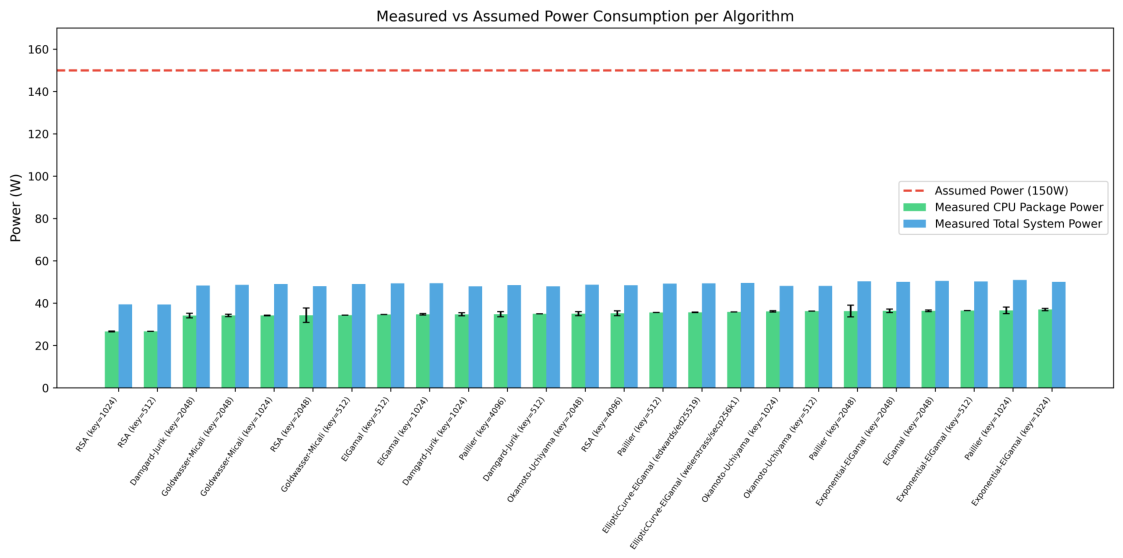
Overall average	—	34.7	48.4	150	4.3×

summarizes the measured power consumption for each algorithm alongside the original 150 W assumption. Across all 750 runs, the average CPU package power was 34.7 W (range: 26.1–40.6 W, std: 2.7 W), and the average total system power, including the idle GPU, memory, and chipset, was 48.4 W (range: 39.4–54.9 W).

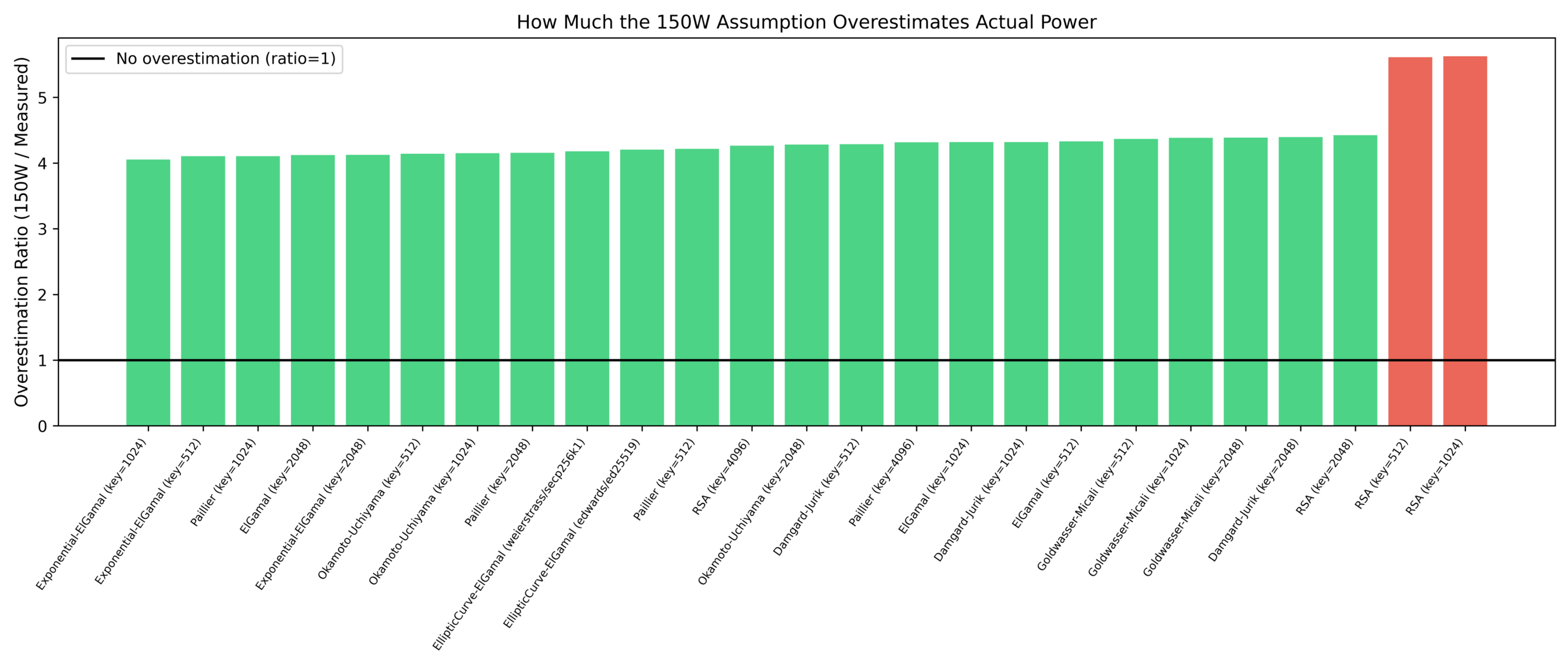
The gap between measured CPU power and the 150 W assumption is substantial: 150 W overestimates CPU-level power by a factor of 4.3. However, as discussed in the transferability analysis below, 150 W may be a reasonable approximation for the total system power on a single-socket rack server. The original manuscript did not specify which power scope the 150 W figure represented, and this ambiguity is itself a methodological weakness that we address in this revision by reporting all three scopes explicitly.

The power variation across algorithms is modest but real: RSA-1024 drew only 26.7 W on average, while Exponential-ElGamal-1024 reached 37.0 W. This difference reflects the distinct instruction profiles of each algorithm. Notably, the idle GPU (NVIDIA RTX Pro 2000) contributed approximately 14 W to the system power (the gap between CPU package power and total system power), mirroring the situation in accelerator-equipped Colab runtimes, where idle accelerator hardware inflates total power readings without participating in PHE computation.

Figure 1 shows the measured CPU and system power per algorithm compared to the 150 W assumption. Figure 2 shows the resulting overestimation ratio.

All carbon emission tables in Section 5.1 and Section 5.2 were originally computed using the 150 W assumption. In the revised manuscript, we present the original estimates alongside calibrated values using the measured 34.7 W average. This allows the reader to assess the impact of the power assumption on all reported carbon figures.

4.3.4. Transferability to Cloud and Data Center Environments

The calibration was performed on a mobile workstation, not a cloud server. This distinction matters because data center servers have higher baseline power consumption due to redundant power supplies, multiple memory channels, storage controllers, network interfaces, and cooling fans. According to the 2024 LBNL United States Data Center Energy Usage Report [7], the average single-socket conventional server drew approximately 118 W over the 2007–2023 period, while dual-socket servers averaged 365 W. A detailed review of server power consumption models based on SPEC data confirms that server power scales nonlinearly with utilization, and that idle power can represent 20–50% of peak power depending on the hardware generation [49].

The empirical server power literature provides additional grounding for the S150 scenario. Idle power in production servers typically accounts for 50 to 70 percent of peak consumption, and the utilization-to-power curve is often super-linear in modern hardware [50,51,52]. Surveys of cloud server power modeling note that fixed single-value assumptions introduce systematic error across utilization regimes, while linear or two-point interpolation models reduce estimation error [53,54,55,56]. A bottom-up decomposition places 150 W in the plausible range for a single-socket rack server under moderate-to-full load: one server-class CPU near its rated TDP (roughly 100 W), ECC DRAM across 8 to 12 channels (roughly 30 W), enterprise NVMe storage (roughly 8 W), and platform baseline covering chipset, voltage regulators, fans, and BMC (roughly 20 W). Masanet et al. further contextualize these numbers by documenting a fourfold reduction in electricity per computation for typical volume servers between 2010 and 2018 [57]. We therefore treat 150 W as a scenario anchored in this literature rather than a single fixed baseline, reporting all three scopes (34.7 W CPU Package, 48.4 W Total System, 150 W S150) together so the reader can navigate between them.

However, the relevant comparison is not full-server power at full load, but the incremental power consumed by a single-threaded Python workload. LightPHE is a pure Python library that uses one CPU core at a time. On our mobile workstation, this single-threaded workload raised CPU package power from approximately 25 W at idle to 35 W under PHE load, an increment of roughly 10 W attributable to the cryptographic computation itself. On a Xeon server, the incremental CPU power for a single-threaded Python task would be comparable, typically 10–20 W above idle, because the per-core power draw depends on the instruction mix and clock frequency rather than the number of inactive cores or peripheral components. Published RAPL-based energy measurements of cryptographic workloads on Intel Core i7 server-class CPUs report similar ranges [58]. An analysis of RAPL measurement methodologies across multiple processor families confirms that RAPL accurately tracks CPU package power for compute-bound workloads [59].

The total system power, which includes idle components, is a separate question. A single-socket server running one PHE thread might draw 120–180 W total, placing the S150 scenario within the plausible range as a total system figure for that class of hardware. Recent energy analysis of cryptographic algorithms in server environments reports total system power in the range of 95–160 W during encryption workloads [60]. The issue is that the original manuscript did not specify whether 150 W referred to CPU-only power, total server power, or some other quantity. In this revision, we explicitly distinguish between three power scopes.

Table 7. Power consumption ranges by platform type and measurement scope; 1S = single-socket, 2S = dual-socket.

Platform Type	CPU Package Power (W)	Total System Power (W)	Source
Mobile workstation (this study)	26–41	39–55	RAPL measurement
Desktop (Core i7)	30–65	80–120	[58]
1S server, idle	20–40	80–120	[7,49]
1S server, single-thread	30–80	100–180	[49,60]
2S server, full load	200–400	400–750	[7,61]
Original assumption	150 W (scope unspecified)		—

summarizes the power consumption ranges for different platform types based on our measurements and published data.

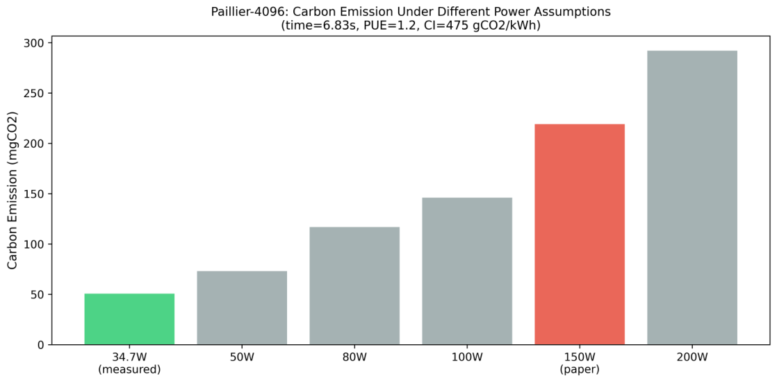
The sensitivity analysis in Section 5.6 tests power assumptions from 34.7 W (measured CPU-only) through 50, 80, 100, 150, and 200 W, covering the full plausible range from CPU-only mobile measurements to total system power on server hardware. This allows readers to select the power figure most appropriate to their deployment scenario and interpret the carbon tables accordingly.

The existing emission tables (Tables S1 and others in the Supplementary Materials) remain computed using the original 150 W assumption, which we hereafter label the S150 server-scenario estimate. As Table 7 shows, 150 W is consistent with total system power for a single-socket server running a single-threaded cryptographic workload. To illustrate the practical impact of the power scope choice,

Table 8. Bridging table: carbon cost under different power scopes (PUE = 1.2, 475 gCO₂/kWh, Scope 3 ratio = 0.35).

Operation	Time (s)	CPU Package (34.7 W) mgCO2	Local System (48.4 W) mgCO2	S150 Server (150 W) mgCO2	S150/CPU Ratio
RSA-2048 keygen	0.438	3.2	4.5	14.0	4.4×
Paillier-4096 keygen	6.833	50.8	70.8	219.1	4.3×
EC-ElGamal secp256k1	0.024	0.2	0.3	0.8	4.3×
Goldwasser–Micali-2048	0.486	3.6	5.1	15.6	4.4×

presents four representative operations with carbon estimates under three power assumptions side by side.

The S150 column reproduces the values used in the emission tables throughout Section 5.2 and the Supplementary Materials. The CPU Package and Local System columns show that the same operations cost under measured power. The ratio column confirms that the S150 assumption scales all carbon values by approximately 4.3× relative to CPU-level measurements. Because this scaling factor is nearly constant across algorithms, the relative ranking between algorithms is preserved regardless of which power scope is used. The sensitivity analysis in Section 5.6 provides the full parameter sweep for readers who need to map these results to a specific deployment scenario.

4.4. Experimental Design and Statistical Protocol

In the original submission, each experiment was repeated 5 times, and only the average was reported. As noted by the reviewers, this is insufficient for cloud environments where execution times can vary due to shared resources, and for algorithms with probabilistic key generation where run-to-run variance is inherently high.

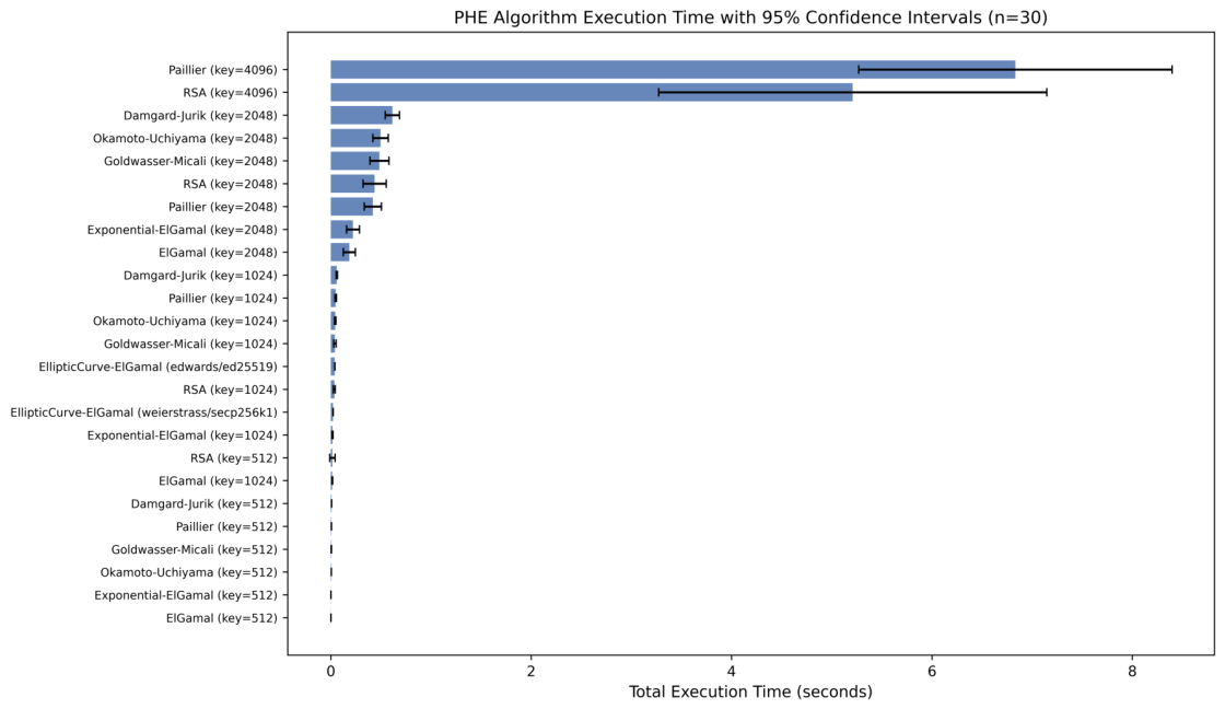
In the calibration experiment, we increased the number of repetitions to 30 for each algorithm and key size combination. For each configuration, we report the following statistics: mean, standard deviation, 95 percent confidence interval (computed via the t-distribution with $n-1$ degrees of freedom), and the coefficient of variation (CV), defined as the ratio of standard deviation to mean expressed as a percentage. A high CV indicates that a single measurement is a poor predictor of the typical value, and that carbon estimates derived from it carry proportionally high uncertainty.

This protocol is applied to the calibration experiment in Section 4.3. The original cloud experiments used 5 repetitions; we acknowledge this as a limitation and present the calibration data as a more statistically grounded reference point.

The execution order within the calibration experiment is sequential rather than randomized, and this is a deliberate methodological choice. Sequential execution preserves CPU cache state, thermal conditions, and memory access patterns across repetitions of the same configuration, which isolates algorithmic variability from scheduling-induced variability. Randomization is the standard choice when the goal is to average over background conditions, but it introduces an additional source of variance that is harder to interpret in per-algorithm energy profiling. Randomized-order benchmarks are a natural complement to the present sequential protocol and are left for future work.

The benchmark scripts, raw timing data, and calibration logs used in this study will be released in the LightPHE GitHub repository under a dedicated revision tag so that the measurements can be reproduced on independent hardware. Exact reproduction of cloud-level numbers is not guaranteed because cloud providers adjust hardware allocations over time, but the relative algorithm ranking and the CV patterns reported here are expected to be stable across different sessions.

5. Results and Discussion

To use the LightPHE framework, the library is imported, and the LightPHE class is initialized with the desired partially homomorphic encryption (PHE) algorithm. The following code example demonstrates this process.

In the example shown in Listing 1, the LightPHE class is imported from the LightPHE library. The algorithms list contains the names of all the supported PHE algorithms. Initializing the LightPHE class with the first algorithm in the list, which corresponds to RSA in this case, generates a random private–public key pair for the chosen cryptosystem. This procedure is sufficient to build a cryptosystem using the selected PHE algorithm.

Listing 1: Building a Cryptosystem.

# install the library if not installed yet !pip install lightphe   # import the library from lightphe import LightPHE   # supported PHE algorithms algorithms = [   “RSA”,   “ElGamal”,   “Goldwasser--Micali”,   “Exponential-ElGamal”,   “EllipticCurve-ElGamal”,   “Paillier”,   “Damgard--Jurik”,   “Okamoto--Uchiyama”,   “Benaloh”,   “Naccache--Stern”, ]   # build cryptosystem with private--public key pair cs = LightPHE(    algorithm_name = algorithms[0],    key_size = 1024, )

Then, the following code demonstrates defining a plaintext value, encrypting it, and then decrypting it to verify correctness.

In the example shown in Listing 2, a plaintext value, m, is defined and set to 17. The encrypt method of the cryptosystem is called with the plaintext value, producing the ciphertext c. The decrypt method of the cryptosystem is then called with the ciphertext as its argument to decrypt the plaintext. An assertion is made to verify that the decrypted value matches the original plaintext m. This ensures that the encryption and decryption processes function correctly within the cryptosystem.

The following code demonstrates homomorphic addition using the Paillier algorithm:

In the example demonstrated in Listing 3, the LightPHE class is initialized with the Paillier algorithm. This generates a random private–public key pair. Two plaintext values, $m_1$ and $m_2$, are defined and set to 10,000, representing the base salary, and 500, representing the wage increase in amount, respectively. The encrypt method of the LightPHE instance cs is called with $m_1$ and $m_2$ as arguments, producing the ciphertexts $c_1$ and $c_2$. Encryption can be done with just public keys, without the need for private keys. These are done on the premises side, and the $c_1$, $c_2$ pair and public keys are sent to the cloud environment.

Listing 2: Encrypt and Decrypt with Built Cryptosystem.

# define plaintext m = 17   # calculate ciphertext with public key c = cs.encrypt(m)   # proof of work - decrypt with private key assert cs.decrypt(c) == m

Listing 3: On-Premises Encryptions.

def encrypt_on_prem() -> Tuple[int, int, dict]:    “““    Build Paillier with random keys & encrypt    Returns:      a tuple of      - c1 (int): 1st ciphertext      - c2 (int): 2nd ciphertext      - public_key (dict): public key    ”””      # on prem builds a Paillier cryptosystem    cs = LightPHE(algorithm_name = “Paillier”)      # on prem defines plaintexts    m1 = 10000 # base salary    m2 = 500 # wage increase in amount      # on prem calculates ciphertexts    c1 = cs.encrypt(m1)    c2 = cs.encrypt(m2)      return (c1.value, c2.value, cs.cs.keys[“public_key”])

Listing 4 summarizes the operations performed on the cloud side. It receives the $c_1$, $c_2$ pair and public keys from the on-premises side. First, the cloud cannot decrypt the $c_1$, $c_2$ pair because it does not have the private key. Second, $c_1$ and $c_2$ are converted to ciphertext objects, and LightPHE overrides the class’s addition method to perform homomorphic addition, as mentioned in Section 4.2. So, homomorphic addition is performed by adding $c_1$ and $c_2$ to produce a new ciphertext, $c_3$, which represents the updated encrypted salary. This operation does not require the private key and can be done using only the public key. Even though $c_3$ was calculated by the cloud system, the cloud itself cannot decrypt it because it does not have the private key. Finally, the cloud stores $c_3$ in its database.

Listing 4: Cloud Calculations.

def perform_homomorphic_operation_on_cloud(   c1: int, c2: int, public_key: dict ) -> int:    “““    Perform homomorphic addition on cloud    Args:      c1 (int): 1st ciphertext      c2 (int): 2nd ciphertext      public_key (dict): public key    Returns:      c3 (int): homomorphic addition of c1 & c2    ”””      # cloud builds same cs with only public key    cs = LightPHE(      algorithm_name = “Paillier”,      keys = public_key    )      # cloud casts c1 and c2 to ciphertext objects    c1 = cs.create_ciphertext_obj(c1)    c2 = cs.create_ciphertext_obj(c2)      def confirm_decrypt_not_possible(ciphertext):       with pytest.raises(        ValueError,        match=“You must have private key”       ):         cs.decrypt(ciphertext)      # confirm that cloud cannot decrypt c1 and c2    confirm_decrypt_not_possible(c1)    confirm_decrypt_not_possible(c2)      # still cloud can perform homomorphic addition    c3 = c1 + c2      # confirm that cloud cannot decrypt c3    confirm_decrypt_not_possible(c3)      return c3.value

   After that, Listing 5 summarizes the proof of work. The on-premises side retrieves $c_3$ from the cloud. An assertion is made to verify that decrypting $c_3$ returns the sum of the original plaintext values ($m_1$ + $m_2$) on the on-premises side. Decryption can only be performed by the data owner, who holds the private key. This demonstrates the correctness of the homomorphic addition operation.

Listing 5: Proof of Work.

# c3 was calculated by the cloud # on prem has a private key to perform decryption assert cs.decrypt(c3) == m1 + m2

   In the example illustrated in Listing 6, a scalar k is defined to represent a 5% wage increase and is set to 1.05. The variable $c_1$ is a type of ciphertext, representing the encrypted base salary of someone, and the class’s right multiplication method is overridden to perform scalar multiplication. So, scalar multiplication is performed by multiplying k with the ciphertext $c_1$ to produce a new ciphertext $c_4$, which represents the encrypted updated salary. This operation does not require the private key and can be done by anyone who has the public keys.

Listing 6: Scalar Multiplication.

# build Paillier - it’s additively homomorphic cs = LightPHE(algorithm_name = “Paillier”)   # define base salary on prem m1 = 10000   # find encrypted base salary on prem c1 = cs.encrypt(m1)   # set 5% wage increase percentage as constant # on prem or in cloud k = 1.05   # calculate encrypted updated salary in cloud # private key is not required! c4 = k ∗ c1   # proof of work on prem - decrypt /w private key assert cs.decrypt(c4) == k ∗ m1

Finally, an assertion is made to verify that decrypting $c_4$ returns the product of the scalar, k, and the original plaintext $m_1$, demonstrating the correctness of the scalar multiplication operation. This verification can only be performed by the data owner, who holds the private key of the cryptosystem.

The following code in Listing 7 demonstrates the limitations of the Paillier algorithm with respect to multiplicative and exclusive homomorphic operations:

Listing 7: Unsupported Operations Raise Errors.

# paillier is not multiplicatively homomorphic with pytest.raises(ValueError):  c3 = c1 ∗ c2   # paillier is not homomorphic with respect to XOR with pytest.raises(ValueError):  c4 = c1 ^ c2

Since the Paillier algorithm is not multiplicatively homomorphic, attempting to multiply ciphertexts $c_1$ and $c_2$ will raise an error with the message “Paillier is not homomorphic with respect to the multiplication”. Similarly, since Paillier is not homomorphic with respect to XOR, attempting to perform an exclusive OR operation on $c_1$ and $c_2$ will raise another error with the message “Paillier is not homomorphic with respect to the exclusive or”. These are raised by the Paillier class’s homomorphic multiply and homomorphic XOR methods. These exceptions make the algorithm’s limitations with respect to unsupported operations explicit.

5.1. Performance

Before reporting performance numbers,

Table 9. NIST’s key size recommendations.

Symmetric Key Size	RSA Variants Key Size Equivalent	ECC Key Size Equivalent	Expected Lifetime
80	1024	160	Until 2010
112	2048	224	Until 2030
128	3072	256	Beyond 2030
192	7680	384	Much Beyond 2030
256	15360	521	Much Beyond 2030

summarizes the National Institute of Standards and Technology (NIST) recommendations for key sizes at each security level. The provided

Table 10. Time consumption of algorithms with 80-bit symmetric-key-size equivalents, in seconds.

Algorithm	Key Size	Key Generation	Encrypt	Decrypt	Homomorphic Operation
RSA	1024	0.1483	0.00305	0.0038	$1.70708\times {10}^{-5}$
ElGamal	1024	0.0177	0.00132	0.0007	$1.66416\times {10}^{-5}$
Paillier	1024	0.0507	0.01162	0.0120	$1.90258\times {10}^{-5}$
Damgård–Jurik	1024	0.0585	0.02356	0.0245	$3.82900\times {10}^{-5}$
Okamoto–Uchiyama	1024	0.1050	0.01148	0.0037	$1.82629\times {10}^{-5}$
Goldwasser–Micali	1024	0.0400	0.00027	0.0093	$6.70433\times {10}^{-5}$
Exponential-ElGamal	1024	0.0302	0.00109	3.1553	$1.03474\times {10}^{-5}$
EllipticCurve-ElGamal	160	0.0053	0.01010	4.1529	$6.82354\times {10}^{-5}$

,

Table 11. Time consumption of algorithms with 112-bit symmetric-key-size equivalents, in seconds.

Algorithm	Key Size	Key Generation	Encrypt	Decrypt	Homomorphic Operation
RSA	2048	1.4959	0.0215	0.0235	$5.04017\times {10}^{-5}$
ElGamal	2048	0.6238	0.00716	0.0037	$1.92165\times {10}^{-5}$
Paillier	2048	0.7613	0.0851	0.0847	$5.97000\times {10}^{-5}$
Damgård–Jurik	2048	0.6388	0.1727	0.1997	$1.04141\times {10}^{-4}$
Okamoto–Uchiyama	2048	0.7543	0.0781	0.0239	$3.19004\times {10}^{-5}$
Goldwasser–Micali	2048	0.6725	0.00067	0.0536	$1.94454\times {10}^{-4}$
Exponential-ElGamal	2048	0.3957	0.00695	10.572	$1.69277\times {10}^{-5}$
EllipticCurve-ElGamal	224	0.0060	0.00862	3.6356	$5.64575\times {10}^{-5}$

,

Table 12. Time consumption of algorithms with 128-bit symmetric-key-size equivalents, in seconds.

Algorithm	Key Size	Key Generation	Encrypt	Decrypt	Homomorphic Operation
RSA	3072	5.8871	0.0886	0.1201	$4.106\times {10}^{-5}$
ElGamal	3072	1.5976	0.0253	0.0120	$3.009\times {10}^{-5}$
Paillier	3072	2.5762	0.3211	0.3188	$1.361\times {10}^{-4}$
Damgård–Jurik	3072	3.0325	0.6973	0.6809	$2.054\times {10}^{-4}$
Okamoto–Uchiyama	3072	2.7635	0.2815	0.0881	$6.485\times {10}^{-5}$
Goldwasser–Micali	3072	3.6569	0.0011	0.4216	$3.805\times {10}^{-4}$
Exponential-ElGamal	3072	1.6232	0.0214	23.171	$2.503\times {10}^{-5}$
EllipticCurve-ElGamal	256	0.0086	0.0119	4.3759	$7.157\times {10}^{-5}$

and

Table 13. Time consumption of algorithms with a 192-bit symmetric key size, equivalent in seconds.

Algorithm	Key Size	Key Generation	Encrypt	Decrypt	Homomorphic Operation
RSA	7680	370.568	0.8109	0.9861	$1.1673\times {10}^{-4}$
ElGamal	7680	22.1267	0.2702	0.1383	$7.1764\times {10}^{-5}$
Paillier	7680	71.0874	3.9756	4.0049	$5.4407\times {10}^{-4}$
Damgård–Jurik	7680	110.567	8.0903	8.1464	$1.0164\times {10}^{-3}$
Okamoto–Uchiyama	7680	84.0547	3.8247	1.1667	$2.6650\times {10}^{-4}$
Goldwasser–Micali	7680	78.9467	0.00583	4.1952	$2.1928\times {10}^{-3}$
Exponential-ElGamal	7680	49.9941	0.2669	117.68	$7.1144\times {10}^{-5}$
EllipticCurve-ElGamal	384	0.01000	0.00717	3.5553	$5.3978\times {10}^{-5}$

then present the performance metrics of various cryptographic algorithms with default configurations, specifically focusing on key generation, encryption, decryption, and homomorphic operations such as addition, multiplication, or XOR with different key sizes. These measurements are important for evaluating the practicality and efficiency of these algorithms in real-world applications. Here, the encryption and homomorphic operation times are represented in scientific notation to illustrate the performance differences clearly. The values in cells represent the times in seconds and are the average of five runs from the original cloud experiments. The calibration experiment in Section 4.3 uses 30 repetitions per configuration for stronger statistical grounding.

In these experiments, 18-bit plaintexts were used to simulate realistic annual salary values, typically ranging in the hundreds of thousands. This choice reflects a practical application scenario where the encryption of such values is relevant.

The tables also adhere to the National Institute of Standards and Technology (NIST) recommendations for key sizes to achieve specific security levels [62] as detailed in Table 9. For an 80-bit symmetric key security level, NIST suggests using 160-bit keys for elliptic curve cryptography (ECC) and 1024-bit keys for other algorithms. For a 112-bit symmetric key security level, 224-bit ECC keys and 2048-bit keys for other algorithms are recommended. For a 128-bit symmetric key security level, NIST recommends 256-bit ECC keys and 3072-bit keys for other algorithms. These guidelines ensure that the cryptographic strength meets the required security standards. We include 80-bit results for historical comparison and to show the energy scaling trend across security levels. Per NIST SP 800-131A Rev. 2, 80-bit security is no longer approved for general use, so practitioners should treat the 128-bit results as the primary reference for deployment decisions.

For the Elliptic Curve ElGamal scheme, although the implementation supports multiple curve forms and parameter sets, we specifically employed the Weierstrass form instantiated with MNT3-1 (160-bit), P-224 (224-bit), secp256k1 (256-bit), and P-384 (384-bit) curves. This choice ensures compatibility with widely adopted cryptographic libraries and provides an estimated 128-bit security level under standard assumptions. The curve parameters were used in their standard form without additional optimizations. Note that performance characteristics may vary across different curve models (e.g., Edwards or Koblitz forms) due to differences in arithmetic efficiency.

One notable observation from the tables is the much higher decryption times for the Elliptic Curve ElGamal and Exponential ElGamal algorithms, particularly at smaller key sizes. This is attributable to the necessity of solving the discrete logarithm problem (DLP) and the elliptic curve discrete logarithm problem (ECDLP) during decryption. This computational complexity renders these cryptosystems more theoretical than practical, especially given the small plaintext values used in the experiments. As the plaintext size increases, the decryption times are expected to rise even further, exacerbating the impracticality.

What stands out is that larger key sizes do not have a major impact on the encryption and decryption times of Elliptic Curve ElGamal. This consistency across different key sizes is worth attention. Still, the decryption time for Elliptic Curve ElGamal remains slow when compared to other cryptosystems, making it less practical with today’s computational power for applications requiring frequent decryption at the 80, 112, and 128-bit symmetric-key-size equivalents. At the 192-bit symmetric-key-size equivalents, though, Elliptic Curve ElGamal becomes advantageous, as it becomes faster in key generation, encryption, and decryption when compared to other additively homomorphic encryption algorithms such as Paillier or Damgård–Jurik. Beyond that, Elliptic Curve ElGamal offers strong classical security at smaller key sizes and more predictable performance scaling. While key generation, encryption, and decryption times grow super-linearly with key size in other schemes, EC-ElGamal shows approximately linear growth because the dominant cost is scalar multiplication on a fixed curve rather than modular arithmetic on increasingly large integers. We note, however, that EC-based schemes are not post-quantum resistant, since the elliptic curve discrete logarithm problem is polynomial-time solvable by Shor’s algorithm. The advantage of EC-ElGamal in this study is efficiency under the classical threat model, not quantum resistance. In this sense, it serves as a baseline against which future PQC-based homomorphic schemes can be compared.

The Benaloh and Naccache–Stern cryptosystems were excluded from these experiments. Although the implementation issues were resolved and both schemes are now operational, key generation remains unreliable. In particular, the key generation procedure may fail to produce valid parameters within a predefined limit, for instance, max_tries = 10,000, resulting in non-deterministic termination and runtime errors. Due to this instability and limited practical feasibility at higher security levels, these cryptosystems were excluded from the comparative evaluation.

As shown in the tables, homomorphic operations and encryption are very fast. This matters in practice because these operations are typically handled frequently, with encryption being performed on-premises and homomorphic operations executed in the cloud. In cloud environments, where performance is a key concern, the swift execution of these tasks keeps the system running well. Although decryption is slower than both homomorphic operations and encryption, its less frequent occurrence mitigates the impact of its slower speed. Key generation occurs only once, and while it may be slightly slower, its infrequent occurrence makes this delay negligible in the overall scheme of cryptographic processes.

Overall, these tables provide valuable insights into the performance and practicality of various cryptographic algorithms under different security settings, emphasizing the balance between theoretical capabilities and real-world applicability.

Finally, the original cloud timing experiments reported in Table 10, Table 11, Table 12 and Table 13 were collected on a system with an 11th Gen Intel Core i7-11370H CPU, whereas the power calibration experiment in Section 4.3 was conducted separately on a Dell Pro Max 16 with an Intel Core Ultra 9 285H.

5.2. Cloud Performance

We conducted experiments on key generation, encryption, decryption, and homomorphic operations using various algorithms with an equivalent 192-bit symmetric key size. These experiments were performed across several cloud environments, including Colab-CPU, Colab-A100, Colab-L4, Colab-T4, Colab-TPU2, and Azure Spark, running five experiments for each task and averaging the consumption times to reduce variance. An important caveat applies throughout this section: LightPHE is a pure Python library that runs all cryptographic operations on the CPU. None of the GPU or TPU resources in the labeled environments were directly used for PHE computations. The performance differences observed across these environments reflect differences in the accompanying CPU and memory subsystems, not GPU or TPU acceleration. LightPHE is available as an open-source Python library (MIT license) at https://github.com/serengil/lightphe (accessed on 1 February 2026) and can be installed via pip. All cloud environments used in this study, including all five Google Colab runtimes and Microsoft Azure Spark, are publicly accessible, allowing researchers to reproduce our experimental setup and results.

A note on variability is in order. Google Colab reassigns virtual machines across sessions and sometimes within sessions, so repetitions across different runs implicitly sample across different underlying physical hosts and tenant configurations. Therefore, the coefficient of variation values reported in Section 4.4 and Section 5.3 reflect both algorithmic execution-time variability and cloud-environment variability, and these two sources cannot be fully separated without coordinated bare-metal access across providers. The calibration experiment in Section 4.3, conducted on a single bare-metal workstation, isolates the algorithmic component of this variability for the 25 configurations it covers.

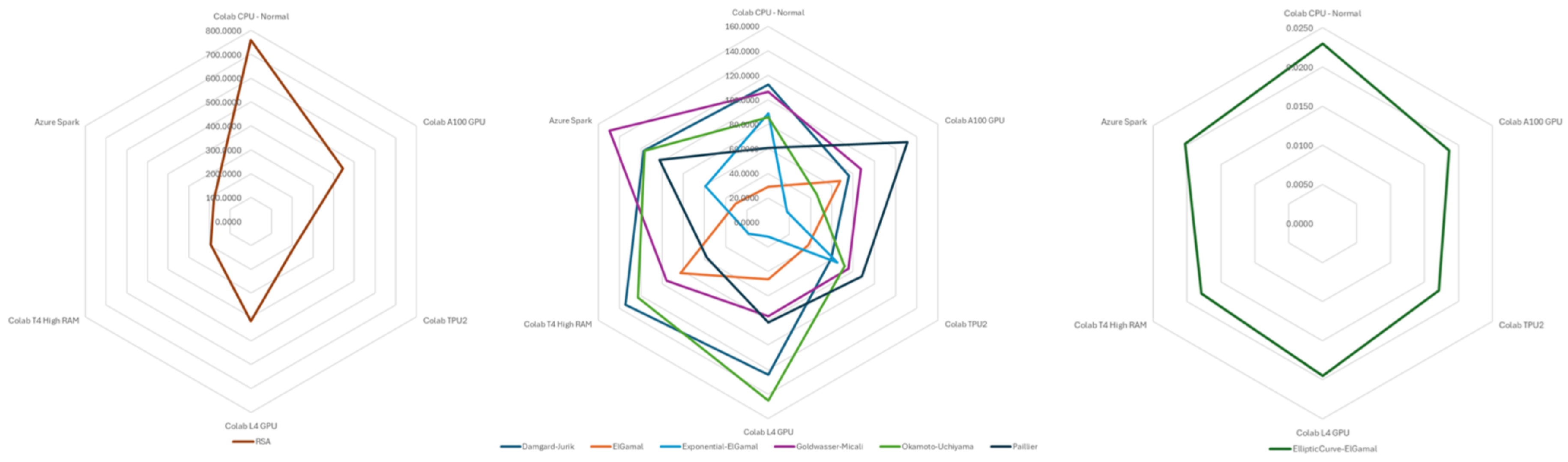
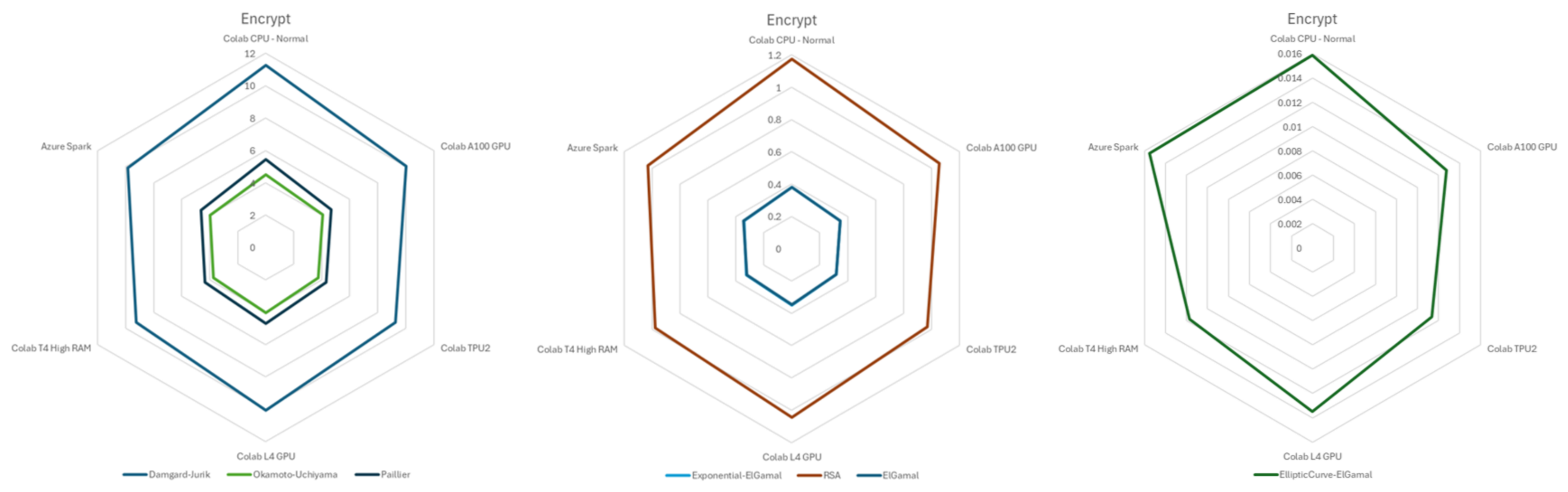
We use radar map charts to present the performance of various algorithms across diverse cloud environments. Multiple radar maps are shown because consolidating them into a single radar map would render it illegible. The radar maps are also arranged from left to right to illustrate slower to faster speeds.

Figure 3 illustrates a radar map depicting key generation times in seconds for different algorithms across various cloud environments. Among these algorithms, RSA emerges as the slowest in key generation, with Elliptic Curve ElGamal demonstrating the fastest performance. Following Elliptic Curve ElGamal, ElGamal and Exponential ElGamal exhibit slightly slower key generation times than Elliptic Curve ElGamal. The remaining algorithms exhibit relatively similar performance to each other. One thing that stands out is that key generation shows noticeable instability compared to encryption, decryption, or homomorphic operations. This instability arises from the inherent requirement of generating random values until a specific condition is met, contributing to fluctuating performance levels.

Figure 4 shows the performance comparisons of various algorithms for encryption tasks across different cloud environments, with values depicted in seconds. Damgård–Jurik, Paillier, and Okamoto–Uchiyama were the slowest performers. ElGamal and Exponential ElGamal charts are overlaid, showing moderate performance, with RSA slightly trailing behind in this category. Meanwhile, Elliptic Curve ElGamal emerged as the fastest option.

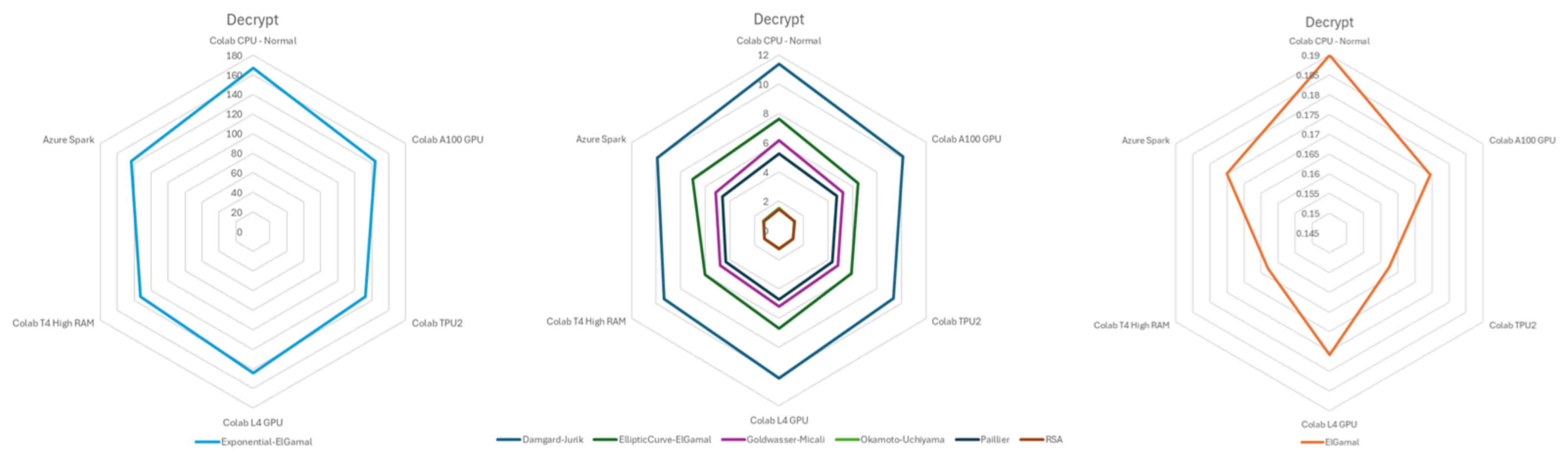
The decryption performance comparison in seconds, shown in Figure 5, revealed Exponential ElGamal as the slowest, ElGamal as the fastest, and other algorithms displaying moderate performance across different cloud environments.

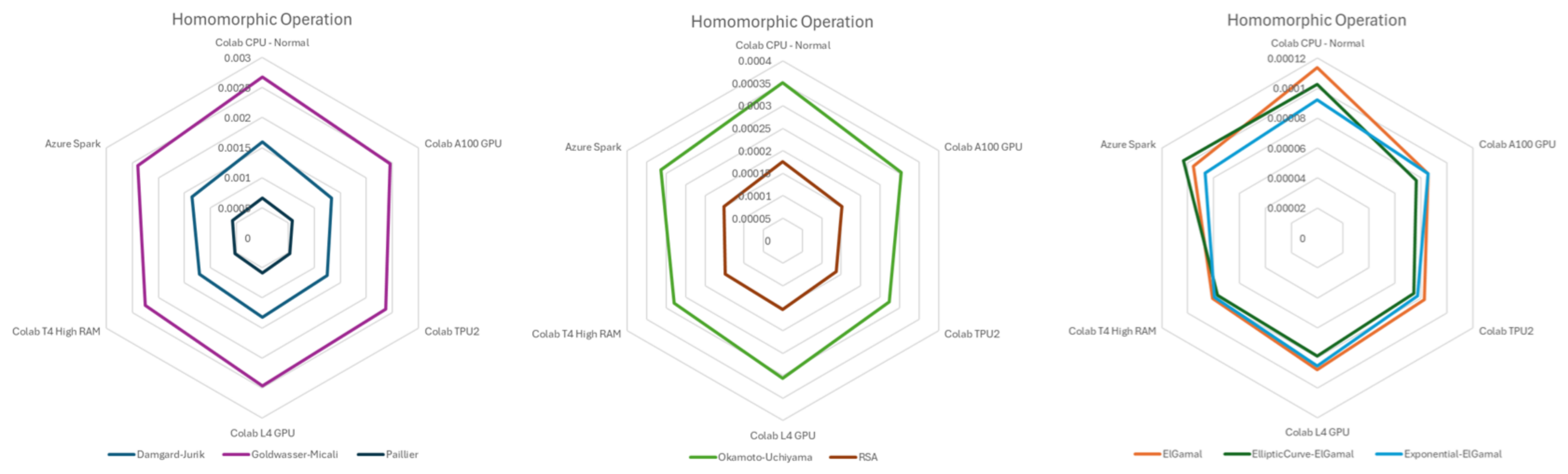
Figure 6 shows the performance of various algorithms for homomorphic operations across different cloud environments, with values depicted in seconds. Damgård–Jurik, Goldwasser–Micali, and Paillier were the slowest, while ElGamal, Exponential ElGamal, and Elliptic Curve ElGamal were the fastest. Okamoto–Uchiyama and RSA demonstrated moderate performance in homomorphic operations. In practice, only the homomorphic operation is performed in the cloud environment, and this operation is performed often.

In evaluating the performance of various tasks across different cloud environments, it becomes evident that the Colab-CPU environment is the slowest, compared to the much faster performance of Colab-TPU2 and Colab-T4, irrespective of the algorithm employed. The performance of various tasks across different cloud environments is summarized in

Table 14. Cloud Environment Configurations. All Colab instances share an Intel Xeon host CPU (∼2.2 GHz, 2 vCPU). Accelerators listed as “idle” were present in the runtime but not used by LightPHE.

Label	Host CPU	Idle Accelerator	System RAM	Provider
Colab-CPU	Intel Xeon ∼2.2 GHz, 2 vCPU	None	∼13 GB	Google Colab
Colab-A100	Intel Xeon ∼2.2 GHz, 2 vCPU	A100 (idle)	∼40 GB	Google Colab
Colab-TPU2	Intel Xeon ∼2.2 GHz, 2 vCPU	TPU v2 (idle)	∼16 GB	Google Colab
Colab-L4	Intel Xeon ∼2.2 GHz, 2 vCPU	L4 (idle)	∼24 GB	Google Colab
Colab-T4	Intel Xeon ∼2.2 GHz, 2 vCPU	T4 (idle)	∼32 GB	Google Colab
Azure Spark	Varies by cluster	None	Varies	Microsoft Azure

.

Google Colab dynamically assigns CPU models to virtual machines, so the exact SKUs may vary between sessions. At the time of our experiments, all Colab runtimes provided an Intel Xeon host processor with 2 vCPUs at approximately 2.2 GHz base frequency. The accelerator-equipped runtimes paired their GPU or TPU with the same Xeon host CPU, but allocated more system memory. Table 14 lists each environment with its host CPU, idle accelerator, and memory allocation. Azure Spark configurations vary by cluster setup. The local machine experiments in Section 5 used a Dell Pro Max 16 with an Intel Core Ultra 9 285H, as described in that section.

The rationale for including accelerator-labeled runtimes in our benchmark is methodological. In practice, cloud users often provision GPU- or TPU-equipped runtimes for mixed workloads where only parts of the pipeline benefit from acceleration, while other parts, including PHE operations, continue to run on the CPU. Benchmarking PHE across such runtimes reveals how host-CPU allocation and memory subsystems affect execution time in the same Xeon host environment, and how idle accelerator hardware inflates total energy consumption without contributing to PHE computation. This is a deliberate design choice rather than a limitation, because it captures a pattern that real-world cloud users encounter when they select a runtime type without changing their code.

As noted earlier, LightPHE is implemented as a pure Python library, meaning the cryptographic operations, such as modular exponentiation and large-integer arithmetic used in RSA, Paillier, and other PHE algorithms, are executed on the CPU rather than offloaded to GPUs or TPUs. No GPU-specific optimizations, such as CUDA-based parallelization or custom memory management strategies for GPU architectures like the NVIDIA A100, were applied. The accelerator-equipped environments, Colab-A100, Colab-L4, and Colab-T4, were selected because they represent commonly available cloud configurations that organizations typically provision. In these setups, the accompanying CPU and system memory characteristics differ from the Colab-CPU environment, which in turn affects the execution performance of CPU-bound Python workloads. As a result, the observed performance differences across accelerator-labeled environments reflect variations in the underlying CPU allocation and memory subsystems rather than direct accelerator use of the PHE algorithms. Exploring GPU-accelerated implementations of specific PHE operations, for instance, through CUDA-based big-integer arithmetic libraries, remains an interesting direction for future work and falls outside the scope of this study. There is one more consideration: in accelerator-equipped runtimes, the GPU or TPU still draws idle power even when it is not used by LightPHE. This idle draw, typically in the range of 30 to 60 watts for modern data center GPUs, adds to the total energy consumption of the machine and, by extension, to its carbon footprint. Our emission model does not currently account for this idle GPU overhead, which means the CO₂ estimates for accelerator-equipped runtimes may slightly understate the true cost. This is a limitation of the current analysis.

For the calculations, each cryptographic operation (key generation, encryption, decryption, and homomorphic operation) is timed, and an estimation-based model, not direct hardware-level power measurement, is used to derive its approximate energy consumption and carbon footprint. No tools such as Intel RAPL, NVIDIA NVML, or external power meters were used. Instead, each operation’s measured wall-clock duration is combined with assumed power and utilization parameters to produce energy estimates. First, the duration of the operation ($\mathit{duration}$) is combined with a fixed CPU utilization factor ($\mathit{cpu}\_\mathit{utilization}$) that is set for each type of operation (e.g., 95%, 85%, etc.). Next, the server’s base power consumption ($\mathit{BASE}\_\mathit{POWER}$, set to 150 W for all scenarios) is used to compute the approximate energy consumption ($\mathit{energy}\_\mathit{wh}$) in watt-hours (Wh), as follows:

$$\mathrm{energy}\_\mathrm{wh}={\displaystyle \frac{\mathrm{BASE}\_\mathrm{POWER}\times \mathrm{cpu}\_\mathrm{utilization}\times \mathrm{duration}\left(\mathrm{s}\right)}{3600}}.$$

All energy values in the per-operation summary table (

Table 15. Energy and carbon per single operation at 128-bit security (DC1, Colab-L4). Values computed using a 150 W server-scenario power assumption (S150); see Section 5.6 for calibrated estimates under alternative power assumptions.

Algorithm	Key Size	Operation	Duration (s)	Energy (Wh)	CO2 (mgCO2)	Wh/Security-Bit
RSA	3072	Key Gen	9.261	0.4765	400.29	0.003723
RSA	3072	Encrypt	0.080	0.0037	3.09	0.000029
RSA	3072	Decrypt	0.093	0.0043	3.59	0.000033
Paillier	3072	Key Gen	3.487	0.1794	150.73	0.001402
Paillier	3072	Encrypt	0.333	0.0154	12.89	0.000120
Paillier	3072	Decrypt	0.336	0.0155	12.99	0.000121
EC-ElGamal	256	Key Gen	0.012	0.0006	0.53	0.000005
EC-ElGamal	256	Encrypt	0.012	0.0006	0.47	0.000004
EC-ElGamal	256	Decrypt	5.887	0.2711	227.69	0.002118
Exp-ElGamal	3072	Key Gen	1.696	0.0873	73.30	0.000682
Exp-ElGamal	3072	Encrypt	0.027	0.0012	1.03	0.000010
Exp-ElGamal	3072	Decrypt	28.011	1.2897	1083.31	0.010075

) and in the emission tables (

Table 16. Cloud Emission Calculations 80-bit, Representative Data Centers (DC1: Carbon, DC4: Renewable, DC7: Hybrid). All values are S150 scenario estimates computed using a fixed 150 W server-level power assumption. Energy is in Wh; emission values are in mgCO₂. See Section 5.6 for the effect of alternative power assumptions. Complete data for all data centers is provided in Supplementary Tables.

Data Center	Algorithm	Key Size	Op.	Dur. (s)	Energy (Wh)	Sc.1 (mgCO2)	Sc.2 (mgCO2)	Sc.3 (mgCO2)	Total (mgCO2)
DC1	RSA	1024	KG	0.2274	0.0117	0.35	7.02	2.46	9.83
DC1	RSA	1024	E	0.004	0.000186	0.01	0.11	0.04	0.16
DC1	RSA	1024	D	0.0045	0.000209	0.01	0.13	0.04	0.18
DC1	RSA	1024	H	0	0	0	0	0	0
DC1	ElGamal	1024	KG	0.0275	0.001417	0.04	0.85	0.3	1.19
DC1	ElGamal	1024	E	0.0015	0.000071	0	0.04	0.01	0.06
DC1	ElGamal	1024	D	0.0009	0.00004	0	0.02	0.01	0.03
DC1	ElGamal	1024	H	0	0	0	0	0	0
DC1	Paillier	1024	KG	0.0439	0.002259	0.07	1.36	0.47	1.9
DC1	Paillier	1024	E	0.0149	0.000686	0.02	0.41	0.14	0.58
DC1	Paillier	1024	D	0.0151	0.000695	0.02	0.42	0.15	0.58
DC1	Paillier	1024	H	0	0.000001	0	0	0	0
DC1	Damgård–Jurik	1024	KG	0.0654	0.003365	0.1	2.02	0.71	2.83
DC1	Damgård–Jurik	1024	E	0.0314	0.001445	0.04	0.87	0.3	1.21
DC1	Damgård–Jurik	1024	D	0.0315	0.001452	0.04	0.87	0.3	1.22
DC1	Damgård–Jurik	1024	H	0	0.000002	0	0	0	0
DC1	Okamoto–Uchiyama	1024	KG	0.076	0.003909	0.12	2.35	0.82	3.28
DC1	Okamoto–Uchiyama	1024	E	0.0139	0.000641	0.02	0.38	0.13	0.54
DC1	Okamoto–Uchiyama	1024	D	0.0047	0.000218	0.01	0.13	0.05	0.18
DC1	Okamoto–Uchiyama	1024	H	0	0.000001	0	0	0	0
DC1	Goldwasser–Micali	1024	KG	0.1013	0.005211	0.16	3.13	1.09	4.38
DC1	Goldwasser–Micali	1024	E	0.0004	0.00002	0	0.01	0	0.02
DC1	Goldwasser–Micali	1024	D	0.0228	0.001052	0.03	0.63	0.22	0.88
DC1	Goldwasser–Micali	1024	H	0.0001	0.000003	0	0	0	0
DC1	Exponential-ElGamal	1024	KG	0.0158	0.000811	0.02	0.49	0.17	0.68
DC1	Exponential-ElGamal	1024	E	0.0016	0.000074	0	0.04	0.02	0.06
DC1	Exponential-ElGamal	1024	D	4.6008	0.21183	6.35	127.1	44.48	177.94
DC1	Exponential-ElGamal	1024	H	0	0	0	0	0	0
DC1	EllipticCurve-ElGamal	160	KG	0.0075	0.000388	0.01	0.23	0.08	0.33
DC1	EllipticCurve-ElGamal	160	E	0.0132	0.000609	0.02	0.37	0.13	0.51
DC1	EllipticCurve-ElGamal	160	D	6.0519	0.27864	8.36	167.18	58.51	234.06
DC1	EllipticCurve-ElGamal	160	H	0.0001	0.000003	0	0	0	0
DC4	RSA	1024	KG	0.0996	0.004336	0	0	0.15	0.15
DC4	RSA	1024	E	0.0041	0.000159	0	0	0.01	0.01
DC4	RSA	1024	D	0.0046	0.000178	0	0	0.01	0.01
DC4	RSA	1024	H	0	0	0	0	0	0
DC4	ElGamal	1024	KG	0.0464	0.002021	0	0	0.07	0.07
DC4	ElGamal	1024	E	0.0016	0.000062	0	0	0	0
DC4	ElGamal	1024	D	0.0009	0.000034	0	0	0	0
DC4	ElGamal	1024	H	0	0	0	0	0	0
DC4	Paillier	1024	KG	0.0755	0.003289	0	0	0.12	0.12
DC4	Paillier	1024	E	0.0151	0.000588	0	0	0.02	0.02
DC4	Paillier	1024	D	0.0152	0.000592	0	0	0.02	0.02
DC4	Paillier	1024	H	0	0.000001	0	0	0	0
DC4	Damgård–Jurik	1024	KG	0.0629	0.002738	0	0	0.1	0.1
DC4	Damgård–Jurik	1024	E	0.0317	0.001234	0	0	0.04	0.04
DC4	Damgård–Jurik	1024	D	0.0317	0.001237	0	0	0.04	0.04
DC4	Damgård–Jurik	1024	H	0	0.000001	0	0	0	0
DC4	Okamoto–Uchiyama	1024	KG	0.0762	0.00332	0	0	0.12	0.12
DC4	Okamoto–Uchiyama	1024	E	0.0139	0.000541	0	0	0.02	0.02
DC4	Okamoto–Uchiyama	1024	D	0.0046	0.00018	0	0	0.01	0.01
DC4	Okamoto–Uchiyama	1024	H	0	0	0	0	0	0
DC4	Goldwasser–Micali	1024	KG	0.086	0.003746	0	0	0.13	0.13
DC4	Goldwasser–Micali	1024	E	0.0004	0.000017	0	0	0	0
DC4	Goldwasser–Micali	1024	D	0.024	0.000937	0	0	0.03	0.03
DC4	Goldwasser–Micali	1024	H	0.0001	0.000003	0	0	0	0
DC4	Exponential-ElGamal	1024	KG	0.0267	0.001162	0	0	0.04	0.04
DC4	Exponential-ElGamal	1024	E	0.0017	0.000065	0	0	0	0
DC4	Exponential-ElGamal	1024	D	4.6526	0.181258	0	0	6.34	6.34
DC4	Exponential-ElGamal	1024	H	0	0	0	0	0	0
DC4	EllipticCurve-ElGamal	160	KG	0.0071	0.000309	0	0	0.01	0.01
DC4	EllipticCurve-ElGamal	160	E	0.0122	0.000476	0	0	0.02	0.02
DC4	EllipticCurve-ElGamal	160	D	5.9941	0.233522	0	0	8.17	8.17
DC4	EllipticCurve-ElGamal	160	H	0.0001	0.000002	0	0	0	0
DC7	RSA	1024	KG	0.2148	0.011051	0.07	1.33	1.16	2.55
DC7	RSA	1024	E	0.004	0.000186	0	0.02	0.02	0.04
DC7	RSA	1024	D	0.0046	0.00021	0	0.03	0.02	0.05
DC7	RSA	1024	H	0	0	0	0	0	0
DC7	ElGamal	1024	KG	0.0535	0.002751	0.02	0.33	0.29	0.64
DC7	ElGamal	1024	E	0.0015	0.000071	0	0.01	0.01	0.02
DC7	ElGamal	1024	D	0.0008	0.000039	0	0	0	0.01
DC7	ElGamal	1024	H	0	0	0	0	0	0
DC7	Paillier	1024	KG	0.0936	0.004818	0.03	0.58	0.51	1.11
DC7	Paillier	1024	E	0.0152	0.000698	0	0.08	0.07	0.16
DC7	Paillier	1024	D	0.0152	0.000702	0	0.08	0.07	0.16
DC7	Paillier	1024	H	0	0.000001	0	0	0	0
DC7	Damgård–Jurik	1024	KG	0.0598	0.003079	0.02	0.37	0.32	0.71
DC7	Damgård–Jurik	1024	E	0.0312	0.001437	0.01	0.17	0.15	0.33
DC7	Damgård–Jurik	1024	D	0.0314	0.001446	0.01	0.17	0.15	0.33
DC7	Damgård–Jurik	1024	H	0	0.000002	0	0	0	0
DC7	Okamoto–Uchiyama	1024	KG	0.112	0.005763	0.03	0.69	0.61	1.33
DC7	Okamoto–Uchiyama	1024	E	0.0139	0.00064	0	0.08	0.07	0.15
DC7	Okamoto–Uchiyama	1024	D	0.0047	0.000215	0	0.03	0.02	0.05
DC7	Okamoto–Uchiyama	1024	H	0	0	0	0	0	0
DC7	Goldwasser–Micali	1024	KG	0.0985	0.00507	0.03	0.61	0.53	1.17
DC7	Goldwasser–Micali	1024	E	0.0004	0.000019	0	0	0	0
DC7	Goldwasser–Micali	1024	D	0.0234	0.001079	0.01	0.13	0.11	0.25
DC7	Goldwasser–Micali	1024	H	0.0001	0.000003	0	0	0	0
DC7	Exponential-ElGamal	1024	KG	0.0726	0.003735	0.02	0.45	0.39	0.86
DC7	Exponential-ElGamal	1024	E	0.0016	0.000073	0	0.01	0.01	0.02
DC7	Exponential-ElGamal	1024	D	4.5853	0.211113	1.27	25.33	22.17	48.77
DC7	Exponential-ElGamal	1024	H	0	0	0	0	0	0
DC7	EllipticCurve-ElGamal	160	KG	0.0072	0.000372	0	0.04	0.04	0.09
DC7	EllipticCurve-ElGamal	160	E	0.0119	0.000547	0	0.07	0.06	0.13
DC7	EllipticCurve-ElGamal	160	D	5.893	0.271324	1.63	32.56	28.49	62.68
DC7	EllipticCurve-ElGamal	160	H	0.0001	0.000003	0	0	0	0

and

Table 17. Cloud emission calculations 128-bit, representative data centers (DC1: Carbon, DC4: Renewable, DC7: Hybrid). All values are S150 scenario estimates computed using a fixed 150 W server-level power assumption. Energy is in Wh; emission values are in mgCO₂. See Section 5.6 for the effect of alternative power assumptions. Complete data for all data centers is provided in Supplementary Tables.

Data Center	Algorithm	Key Size	Op.	Dur. (s)	Energy (Wh)	Sc.1 (mgCO2)	Sc.2 (mgCO2)	Sc.3 (mgCO2)	Total (mgCO2)
DC1	RSA	3072	KG	9.2605	0.47653	14.3	285.92	100.07	400.29
DC1	RSA	3072	E	0.08	0.003684	0.11	2.21	0.77	3.09
DC1	RSA	3072	D	0.0929	0.004277	0.13	2.57	0.9	3.59
DC1	RSA	3072	H	0	0.000001	0	0	0	0
DC1	ElGamal	3072	KG	0.7856	0.040426	1.21	24.26	8.49	33.96
DC1	ElGamal	3072	E	0.0271	0.001247	0.04	0.75	0.26	1.05
DC1	ElGamal	3072	D	0.0139	0.00064	0.02	0.38	0.13	0.54
DC1	ElGamal	3072	H	0	0.000001	0	0	0	0
DC1	Paillier	3072	KG	3.4871	0.17944	5.38	107.66	37.68	150.73
DC1	Paillier	3072	E	0.3333	0.015346	0.46	9.21	3.22	12.89
DC1	Paillier	3072	D	0.336	0.01547	0.46	9.28	3.25	12.99
DC1	Paillier	3072	H	0.0001	0.000005	0	0	0	0
DC1	Damgård–Jurik	3072	KG	2.0441	0.105186	3.16	63.11	22.09	88.36
DC1	Damgård–Jurik	3072	E	0.7094	0.032662	0.98	19.6	6.86	27.44
DC1	Damgård–Jurik	3072	D	0.7171	0.033016	0.99	19.81	6.93	27.73
DC1	Damgård–Jurik	3072	H	0.0003	0.00001	0	0.01	0	0.01
DC1	Okamoto–Uchiyama	3072	KG	1.6661	0.085735	2.57	51.44	18	72.02
DC1	Okamoto–Uchiyama	3072	E	0.295	0.013581	0.41	8.15	2.85	11.41
DC1	Okamoto–Uchiyama	3072	D	0.095	0.004374	0.13	2.62	0.92	3.67
DC1	Okamoto–Uchiyama	3072	H	0.0001	0.000003	0	0	0	0
DC1	Goldwasser–Micali	3072	KG	8.5208	0.438466	13.15	263.08	92.08	368.31
DC1	Goldwasser–Micali	3072	E	0.0017	0.000078	0	0.05	0.02	0.07
DC1	Goldwasser–Micali	3072	D	0.4077	0.018771	0.56	11.26	3.94	15.77
DC1	Goldwasser–Micali	3072	H	0.0005	0.00002	0	0.01	0	0.02
DC1	Exponential-ElGamal	3072	KG	1.6957	0.087258	2.62	52.35	18.32	73.3
DC1	Exponential-ElGamal	3072	E	0.0267	0.001231	0.04	0.74	0.26	1.03
DC1	Exponential-ElGamal	3072	D	28.0105	1.28965	38.69	773.79	270.83	1083.31
DC1	Exponential-ElGamal	3072	H	0	0.000001	0	0	0	0
DC1	EllipticCurve-ElGamal	256	KG	0.0122	0.000628	0.02	0.38	0.13	0.53
DC1	EllipticCurve-ElGamal	256	E	0.0122	0.00056	0.02	0.34	0.12	0.47
DC1	EllipticCurve-ElGamal	256	D	5.8872	0.271057	8.13	162.63	56.92	227.69
DC1	EllipticCurve-ElGamal	256	H	0.0001	0.000003	0	0	0	0
DC4	RSA	3072	KG	3.8942	0.16956	0	0	5.93	5.93
DC4	RSA	3072	E	0.0808	0.003149	0	0	0.11	0.11
DC4	RSA	3072	D	0.0934	0.003639	0	0	0.13	0.13
DC4	RSA	3072	H	0	0.000001	0	0	0	0
DC4	ElGamal	3072	KG	0.1506	0.006557	0	0	0.23	0.23
DC4	ElGamal	3072	E	0.0268	0.001042	0	0	0.04	0.04
DC4	ElGamal	3072	D	0.0137	0.000534	0	0	0.02	0.02
DC4	ElGamal	3072	H	0	0.000001	0	0	0	0
DC4	Paillier	3072	KG	1.3062	0.056874	0	0	1.99	1.99
DC4	Paillier	3072	E	0.3308	0.012889	0	0	0.45	0.45
DC4	Paillier	3072	D	0.3319	0.01293	0	0	0.45	0.45
DC4	Paillier	3072	H	0.0001	0.000004	0	0	0	0
DC4	Damgård–Jurik	3072	KG	4.0465	0.176191	0	0	6.17	6.17
DC4	Damgård–Jurik	3072	E	0.7067	0.027533	0	0	0.96	0.96
DC4	Damgård–Jurik	3072	D	0.7098	0.027653	0	0	0.97	0.97
DC4	Damgård–Jurik	3072	H	0.0003	0.000009	0	0	0	0
DC4	Okamoto–Uchiyama	3072	KG	1.8452	0.080343	0	0	2.81	2.81
DC4	Okamoto–Uchiyama	3072	E	0.2959	0.011529	0	0	0.4	0.4
DC4	Okamoto–Uchiyama	3072	D	0.0951	0.003705	0	0	0.13	0.13
DC4	Okamoto–Uchiyama	3072	H	0.0001	0.000002	0	0	0	0
DC4	Goldwasser–Micali	3072	KG	3.9703	0.172873	0	0	6.05	6.05
DC4	Goldwasser–Micali	3072	E	0.0017	0.000065	0	0	0	0
DC4	Goldwasser–Micali	3072	D	0.4082	0.015903	0	0	0.56	0.56
DC4	Goldwasser–Micali	3072	H	0.0005	0.000017	0	0	0	0
DC4	Exponential-ElGamal	3072	KG	0.6002	0.026134	0	0	0.91	0.91
DC4	Exponential-ElGamal	3072	E	0.0268	0.001045	0	0	0.04	0.04
DC4	Exponential-ElGamal	3072	D	27.782	1.08234	0	0	37.88	37.88
DC4	Exponential-ElGamal	3072	H	0	0.000001	0	0	0	0
DC4	EllipticCurve-ElGamal	256	KG	0.0117	0.000509	0	0	0.02	0.02
DC4	EllipticCurve-ElGamal	256	E	0.012	0.000469	0	0	0.02	0.02
DC4	EllipticCurve-ElGamal	256	D	5.6162	0.218798	0	0	7.66	7.66
DC4	EllipticCurve-ElGamal	256	H	0.0001	0.000002	0	0	0	0
DC7	RSA	3072	KG	14.6075	0.751678	4.51	90.2	78.93	173.64
DC7	RSA	3072	E	0.0802	0.003693	0.02	0.44	0.39	0.85
DC7	RSA	3072	D	0.0934	0.0043	0.03	0.52	0.45	0.99
DC7	RSA	3072	H	0	0.000001	0	0	0	0
DC7	ElGamal	3072	KG	0.9031	0.046472	0.28	5.58	4.88	10.74
DC7	ElGamal	3072	E	0.028	0.001289	0.01	0.15	0.14	0.3
DC7	ElGamal	3072	D	0.0142	0.000654	0	0.08	0.07	0.15
DC7	ElGamal	3072	H	0	0.000001	0	0	0	0
DC7	Paillier	3072	KG	3.0224	0.155528	0.93	18.66	16.33	35.93
DC7	Paillier	3072	E	0.3288	0.015137	0.09	1.82	1.59	3.5
DC7	Paillier	3072	D	0.3311	0.015244	0.09	1.83	1.6	3.52
DC7	Paillier	3072	H	0.0001	0.000005	0	0	0	0
DC7	Damgård–Jurik	3072	KG	4.9993	0.257256	1.54	30.87	27.01	59.43
DC7	Damgård–Jurik	3072	E	0.7044	0.032433	0.19	3.89	3.41	7.49
DC7	Damgård–Jurik	3072	D	0.7052	0.032469	0.19	3.9	3.41	7.5
DC7	Damgård–Jurik	3072	H	0.0003	0.00001	0	0	0	0
DC7	Okamoto–Uchiyama	3072	KG	4.7143	0.24259	1.46	29.11	25.47	56.04
DC7	Okamoto–Uchiyama	3072	E	0.2963	0.013641	0.08	1.64	1.43	3.15
DC7	Okamoto–Uchiyama	3072	D	0.0957	0.004406	0.03	0.53	0.46	1.02
DC7	Okamoto–Uchiyama	3072	H	0.0001	0.000002	0	0	0	0
DC7	Goldwasser–Micali	3072	KG	2.6347	0.135577	0.81	16.27	14.24	31.32
DC7	Goldwasser–Micali	3072	E	0.0017	0.000078	0	0.01	0.01	0.02
DC7	Goldwasser–Micali	3072	D	0.4171	0.019204	0.12	2.3	2.02	4.44
DC7	Goldwasser–Micali	3072	H	0.0005	0.00002	0	0	0	0
DC7	Exponential-ElGamal	3072	KG	3.5652	0.183459	1.1	22.02	19.26	42.38
DC7	Exponential-ElGamal	3072	E	0.0271	0.001247	0.01	0.15	0.13	0.29
DC7	Exponential-ElGamal	3072	D	28.0696	1.292371	7.75	155.08	135.7	298.54
DC7	Exponential-ElGamal	3072	H	0	0.000001	0	0	0	0
DC7	EllipticCurve-ElGamal	256	KG	0.012	0.000617	0	0.07	0.06	0.14
DC7	EllipticCurve-ElGamal	256	E	0.0117	0.00054	0	0.06	0.06	0.12
DC7	EllipticCurve-ElGamal	256	D	5.674	0.26124	1.57	31.35	27.43	60.35
DC7	EllipticCurve-ElGamal	256	H	0.0001	0.000003	0	0	0	0

) are reported in Wh, and the corresponding carbon values are in milligrams of CO₂ (mgCO₂). Table 8 reports carbon comparisons in mgCO₂ only.

This quantity is then multiplied by the data center’s Power Usage Effectiveness (PUE) to account for additional overheads, such as cooling and power distribution. Hence,

$$\mathrm{total}\_\mathrm{energy}=\mathrm{energy}\_\mathrm{wh}\times \mathrm{PUE}.$$

Because a fraction of the power may be from renewable sources, the model uses $\mathit{renewable}\_\mathit{percentage}$ to distinguish between renewable and non-renewable energy consumption. The non-renewable portion ($\mathit{non}\_\mathit{renewable}\_\mathit{energy}$) is assigned a CO₂ intensity ($\mathit{grid}\_\mathit{intensity}$, in gCO₂/kWh) to estimate Scope 2 (purchased electricity) emissions. A small fraction of these non-renewable emissions is assumed to come from backup generators ($\times 0.05$), which constitutes Scope 1. Finally, the model adds Scope 3 emissions by multiplying the total energy by a fixed factor of 0.35. This factor is a simplified proxy for the life-cycle emissions associated with hardware manufacturing, transportation, cooling infrastructure, and end-of-life disposal. Published estimates for the embodied-to-operational carbon ratio of data center equipment vary widely, from roughly 0.2 to 0.5, depending on server type, refresh cycle, and utilization [9]. We chose 0.35 as a mid-range value. Because this factor is applied uniformly across all scenarios, it does not affect the relative ranking of algorithms or data centers, only the absolute Scope 3 numbers. The formulas are:

$$\mathrm{scope}1=\mathrm{non}\_\mathrm{renewable}\_\mathrm{energy}\times \mathrm{grid}\_\mathrm{intensity}\times 0.05,$$

$$\mathrm{scope}2=\mathrm{non}\_\mathrm{renewable}\_\mathrm{energy}\times \mathrm{grid}\_\mathrm{intensity},$$

$$\mathrm{scope}3=\mathrm{total}\_\mathrm{energy}\times \mathrm{grid}\_\mathrm{intensity}\times 0.35.$$

A note on Scope 3 is necessary here. In standard greenhouse gas accounting, Scope 3 covers embodied emissions from hardware manufacturing, transportation, facility construction, and end-of-life disposal. These costs are tied to the supply chain rather than to the local electricity grid, so in principle they should not depend on grid carbon intensity. Our formula nevertheless includes $\mathit{grid}\_\mathit{intensity}$ in the Scope 3 term. We made this choice deliberately as a first-order proxy, not as a physical claim. The reasoning is as follows. Data centers in regions with high grid carbon intensity tend to operate within industrial ecosystems where manufacturing, logistics, and infrastructure also carry higher carbon footprints, partly because these regions rely more heavily on carbon-intensive energy across their entire economies [9]. In that sense, grid intensity serves as a rough correlate of the broader carbon context in which hardware is produced and maintained. We recognize that this coupling overestimates Scope 3 in fossil-heavy regions and underestimates it in renewable-heavy ones. However, because the same multiplicative factor is applied uniformly across all scenarios, the relative ranking of algorithms and the directional comparison between data center types remain unaffected. Only the absolute magnitude of the Scope 3 values changes. For readers who prefer a grid-independent formulation, Scope 3 can be recalculated as $\mathrm{total}\_\mathrm{energy}\times F_{\mathrm{embodied}}$, where $F_{\mathrm{embodied}}$ is a fixed embodied carbon factor in gCO₂/kWh. Published estimates for this factor range from approximately 200 to 500 gCO₂/kWh depending on server model, component mix, refresh cycle, and utilization rate [9]. Our choice of 0.35 as a coefficient, when combined with the grid intensities used in Table 5, produces Scope 3 values that fall within this published range for most configurations. In future work, we plan to decouple Scope 3 from grid intensity entirely and adopt region-specific embodied carbon factors based on actual supply chain data.

Summing these yields $\mathrm{total}\_{\mathrm{mgCO}}_2$. Such a model serves as a demonstration rather than an accurate reflection of real-world data-center measurements, since all parameters (PUE, grid intensity, CPU usage patterns) are fixed and not derived from live monitoring. Nevertheless, it provides a comparative view of how varying cryptographic operations and key sizes might drive differences in energy consumption and resulting emissions. As noted earlier, the emission calculations use 80-bit and 128-bit security levels run on Colab-L4, since including all cloud environments and security levels in the emission tables would make the results too complex to visualize. The data encompass multiple data centers categorized as fossil-fuel-powered (DC1-DC3), fully renewable (DC4-DC6), and hybrid (DC7-DC9). For clarity, the main text presents emission results for one representative data center from each category: DC1 (fossil-fuel-powered), DC4 (renewable), and DC7 (hybrid). The complete emission calculations for all ten data center configurations are available as Supplementary Tables. The analysis below draws on all data centers, but the tables in this section focus on these three representative cases, executing operations such as key generation (KG), encryption (E), decryption (D), and homomorphic operations (H) for algorithms including RSA, ElGamal, Paillier, Damgård–Jurik, Okamoto–Uchiyama, Goldwasser–Micali, Exponential ElGamal, and EllipticCurve-ElGamal. Key sizes analyzed are 1024-bit and 160-bit for the 80-bit security level, and 3072-bit and 256-bit for the 128-bit security level, reflecting equivalent security strengths based on computational complexity.

The obtained results show the clear influence of data center energy sources on the carbon footprint of cryptographic operations. Fully renewable data centers (DC4–DC6) exhibit markedly lower carbon emissions due to effectively zero Scope 1 and Scope 2 emissions, leaving only Scope 3 (indirect) emissions, primarily from hardware manufacturing and supply chains. For example, RSA key generation at 1024-bit in DC4 produced only 0.15 mgCO₂, a reduction of approximately 98% when compared to 9.83 mgCO₂ in the fossil fuel-powered DC1. Fossil-fuel-powered data centers (DC1–DC3), by contrast, recorded the highest emissions, predominantly driven by Scope 2. This is best illustrated by RSA 3072-bit key generation in DC1, which emitted 400.29 mgCO₂ in total, 285.92 mgCO₂ of which can be attributed to electricity sourced from fossil fuels. Hybrid data centers (DC7–DC9) demonstrated emission levels that fell between these extremes. Specifically, RSA 1024-bit key generation in DC7 emitted 2.55 mgCO₂, significantly below DC1 but considerably above DC4.

In comparing the energy intensity of different cryptographic tasks, key generation emerged as the most resource-intensive for most algorithms, such as RSA, ElGamal, and Paillier. For instance, RSA 1024-bit key generation in DC1 required 0.0117 Wh (9.83 mgCO₂), whereas encryption and decryption consumed only 0.000186 Wh (0.16 mgCO₂) and 0.000209 Wh (0.18 mgCO₂), respectively. The exceptions were Exponential ElGamal and EllipticCurve-ElGamal, where decryption proved more energy-intensive due to the complexity of homomorphic properties and discrete logarithm-based computations. A prime example is Exponential ElGamal at 1024-bit, for which the decryption phase in DC1 consumed 0.21183 Wh (177.94 mgCO₂), which is over 260 times that of its own key generation. This makes Exponential ElGamal and Elliptic Curve ElGamal unsuitable for workloads with frequent decryption or large plaintext ranges, since their decryption requires solving a discrete logarithm. In practice, these schemes are only viable when the plaintext space is small, say up to a few million, and decryption is infrequent.

Regarding algorithmic efficiency, elliptic curve-based methods stood out for their reduced energy consumption during key generation and encryption. For instance, EllipticCurve-ElGamal at 160-bit in DC1 consumed only 0.000388 Wh (0.33 mgCO₂) for key generation, noticeably lower than RSA 1024-bit’s 0.0117 Wh. Yet decryption costs remained high for these elliptic curve algorithms at larger key sizes: EllipticCurve-ElGamal at 256-bit required 0.271057 Wh (227.69 mgCO₂) in DC1, contrasting sharply with 0.004277 Wh (3.59 mgCO₂) for RSA 3072-bit decryption. On top of that, scaling security levels from 80-bit to 128-bit produced substantial jumps in both energy usage and emissions. RSA key generation, for instance, increased from 0.0117 Wh (9.83 mgCO₂) at 1024-bit in DC1 to 0.47653 Wh (400.29 mgCO₂) at 3072-bit under the S150 scenario, a ratio of approximately 40. This scaling reflects the cubic relationship between RSA key size and key generation time, compounded by the probabilistic nature of prime search. Similarly, Exponential ElGamal decryption escalated sixfold, reaching 1.28965 Wh (1083.31 mgCO₂) at 3072-bit.

Finally, even among data centers sharing the same primary energy source, operational and hardware variations influenced efficiency. An example is RSA 1024-bit key generation in DC2 (fossil-fuel-powered), which was more efficient at 0.007571 Wh (6.89 mgCO₂) than the 0.0117 Wh (9.83 mgCO₂) measured in DC1. These findings point to the critical role of energy sourcing, algorithm selection, and hardware optimizations in determining the overall carbon footprint and energy consumption of cryptographic processes.

Taken together, these results give concrete support for the sustainable cryptography concept introduced in Section 1. Compared to fully homomorphic encryption, which can impose overhead that is several orders of magnitude higher than plaintext processing [12,18], the PHE schemes tested here show a much lighter energy profile at the same security level, making them a practical choice when only additive or multiplicative homomorphy is needed. As expected from general data center energy research, fossil-heavy and renewable-powered facilities show large emissions differences when running the same workload. In our data, this gap reaches up to 98 percent for fully renewable configurations, consistent with the results of carbon-aware scheduling research, where shifting workloads to cleaner grids is one of the most effective ways to cut operational emissions [8]. In our case, algorithm choice, key size, and deployment location all act as independent levers: a careful combination of the three can reduce the carbon cost of a given security target by two or more orders of magnitude without weakening the cryptographic guarantee itself.

Because the emission model is multiplicative, its sensitivity to each parameter can be stated directly. Scope 2 emissions scale linearly with both PUE and grid carbon intensity: doubling PUE from 1.1 to 2.2 would double the total energy input and so double Scope 2, while doubling grid intensity from 300 to 600 gCO₂/kWh doubles the grams of CO₂ per kilowatt-hour of non-renewable electricity. The ten data center configurations in Table 5 already span a wide range for both parameters, with PUE from 1.05 to 1.5 and grid intensity from 50 to 700 gCO₂/kWh. Across that range, the total emission for the same operation varies by roughly two orders of magnitude. For example, RSA 1024-bit key generation emits 9.83 mgCO₂ in DC1 (PUE 1.3, grid 600) but only 0.07 mgCO₂ in DC5 (PUE 1.05, grid 50). Scope 3 is less sensitive to grid composition because it applies a fixed multiplier to total energy regardless of source. In short, for organizations choosing where to run encrypted workloads, grid carbon intensity is the single most influential parameter, followed by PUE and then algorithm choice.

To put the PHE overhead in perspective, it helps to compare it with that of non-homomorphic encryption. Standard RSA encryption at 128-bit security, corresponding to 3072-bit keys, took 0.004 seconds, and consumed roughly 0.000186 Wh in our measurements. AES-256, a symmetric cipher commonly used for bulk data encryption, typically processes data at gigabytes per second on modern CPUs, so a single AES operation would consume several orders of magnitude less energy than any PHE operation. The additional cost of PHE comes from the mathematical structure needed to allow computation on ciphertexts. Our data show that Paillier encryption at the same 128-bit security level took about 0.125 seconds, roughly 30 times longer than standard RSA encryption. This premium is the price of homomorphic capability, and it needs to be weighed against the alternative of decrypting data in the cloud, which would require sharing private keys and would expose plaintext to the cloud provider.

Table 15 presents the per-operation summary for cross-algorithm comparison, reporting energy per single operation in watt-hours and the corresponding carbon cost in mgCO₂ for DC1 at 128-bit security. We also include energy per security-bit, calculated by dividing the operation energy by 128, which allows a size-independent comparison across algorithms. These normalized values let practitioners estimate the cost of a batch workload by multiplying the per-operation figure by the expected number of operations.

The table shows that for workloads dominated by encryption, EC-ElGamal and Exponential ElGamal are the cheapest options in energy terms, at 0.0006 and 0.0012 Wh per encryption, respectively. But if decryption is frequent, Paillier offers a much more balanced profile with roughly 0.015 Wh for both encryption and decryption, even with its heavier encryption step. RSA key generation stands out as the single most expensive operation at 0.4765 Wh, but its encrypt and decrypt costs are among the lowest. The Wh/security-bit column shows that Exponential ElGamal decryption costs about 0.010 Wh per bit of security, making it roughly 1000 times more expensive per security-bit than its own encryption.

5.3. Statistical Analysis of Execution Time Variability

Table 18. Statistical Summary of Total Execution Time (30 Repetitions per Configuration).

Algorithm (Key)	Mean (s)	Std (s)	CV (%)	95% CI Lower	95% CI Upper	Min–Max (s)
RSA (512)	0.017	0.071	424.0	−0.010	0.043	0.002–0.393
RSA (1024)	0.036	0.026	71.0	0.027	0.046	0.002–0.133
RSA (2048)	0.438	0.310	70.8	0.322	0.554	0.054–1.295
RSA (4096)	5.210	5.186	99.5	3.273	7.146	0.335–20.71
Paillier (4096)	6.833	4.190	61.3	5.268	8.397	1.020–17.83
EC-ElGamal (ed25519)	0.041	0.002	4.2	0.040	0.041	0.038–0.045
EC-ElGamal (secp256k1)	0.024	0.001	4.2	0.023	0.024	0.022–0.026

presents representative statistical profiles from the calibration experiment (30 repetitions per configuration), illustrating the contrast in variability between algorithms that use probabilistic key generation and those that do not.

RSA, ElGamal, and Goldwasser–Micali all rely on generating large prime numbers during key creation. Because prime search is a trial-and-error process, the number of candidates tested before finding a suitable prime varies unpredictably from run to run. This leads to high coefficients of variation: RSA at 512 bits showed a CV of 424 percent, RSA at 4096 bits reached 99.5 percent, and ElGamal at 2048 bits reached 85.7 percent. At these variability levels, a single execution time measurement, or an average of just five runs, is a poor predictor of the typical value.

In contrast, Elliptic Curve ElGamal operations follow a deterministic computation path. Point multiplication on a fixed curve always performs the same sequence of operations regardless of the specific key. Both ed25519 and secp256k1 variants showed a CV of just 4.2 percent, meaning their execution time is nearly constant across runs.

This distinction has a direct practical consequence for carbon estimation. If an algorithm’s execution time varies by a factor of five between runs, the associated carbon estimate carries the same uncertainty. For systems that need to predict or budget their energy cost per cryptographic operation, EC-based schemes offer not only lower average cost but also much more predictable cost.

For brevity, Table 18 reports representative configurations; the full calibration summary for all 25 configurations should be provided in the Supplementary Materials. Figure 7 shows execution times for all 25 configurations with 95 percent confidence intervals.

5.4. Security-Normalized Carbon Comparison

Table 10, Table 11, Table 12 and Table 13 compare algorithms at the same key size, but different cryptosystems achieve different security levels for a given key length. Following NIST SP 800-57 Part 1 Rev. 5 (Table 9), a 256-bit elliptic curve key provides 128 bits of security, while RSA requires a 3072-bit key to reach the same level. Comparing RSA-2048 (112-bit security) against EC-ElGamal with secp256k1 (128-bit security), therefore understates the advantage of elliptic curves: the EC variant provides stronger security while being faster.

Table 19. Carbon cost per operation at equivalent security levels (calibrated power, world-average grid).

Security Level	Algorithm	Key Size	Mean Time (s)	Total gCO2 ($\times {10}^{-3}$)
112-bit	RSA	2048	0.438	2.74
112-bit	EC-ElGamal (P-224)	224	0.006	0.04
128-bit	RSA	3072	∼1.49 *	∼9.31
128-bit	EC-ElGamal (secp256k1)	256	0.024	0.15

* Interpolated from RSA-2048 and RSA-4096 measurements using cubic scaling of key generation time with key length.

presents a comparison in which algorithms are grouped by equivalent security level rather than by key size. Carbon values are computed using the calibrated 34.7 W power measurement, a PUE of 1.2, and the world-average carbon intensity of 475 gCO₂/kWh. Scope 3 emissions use a ratio of 0.35.

At the 128-bit security level, EC-ElGamal completes a full operation cycle in 0.024 s, while the estimated time for RSA-3072 is approximately 1.49 s. This means the elliptic curve variant provides 128-bit security at roughly 1.6 percent of the carbon cost of its RSA equivalent. This ratio is driven by the mathematical structure of the underlying operations: modular exponentiation with multi-thousand-bit integers versus point multiplication on a 256-bit curve.

5.5. Operation-Level Basis of the ECC-RSA Energy Asymmetry

The 1.6 percent ratio above is not accidental. It follows from three differences between RSA and elliptic curve schemes at the level of what the CPU actually computes. We walk through them here because the same pattern governs every security level we report in Table 10, Table 11, Table 12 and Table 13.

RSA encryption computes $c=m^{e}modn$ for a k-bit modulus n. Using square-and-multiply, this call needs about ${log}_{2}e$ modular multiplications, and each modular multiplication on k-bit operands costs $O\left(k^2\right)$ bit operations with schoolbook arithmetic, or $O(klogkloglogk)$ with Schönhage-Strassen. For a fixed small public exponent such as $e=65537$, encryption cost scales as $O\left(k^2\right)$. Decryption uses the private exponent d, whose size is close to k, so its cost grows as $O\left(k^3\right)$. Key generation is the heaviest step: it draws random candidates, runs primality tests on each, and repeats until two $k/2$-bit primes are found. The expected number of candidates grows with k by the prime number theorem, and each Miller-Rabin round is itself cubic, so the total cost is close to $O\left(k^4\right)$. This is what makes RSA key generation time jump from 0.438 s at 2048 bits to 370.568 s at 7680 bits in Table 13. EC-ElGamal replaces all of this with point arithmetic. An encryption call evaluates $kP$ for a scalar k of size close to the order n of the curve and a fixed generator P. Double-and-add requires ${log}_{2}k$ point doublings and about ${\displaystyle \frac{1}{2}}{log}_{2}k$ point additions, and each point operation needs a constant number of field multiplications, additions, and one inversion over an ℓ-bit prime field. The per-encryption cost is therefore $O({\ell }^{2}logk)$, and the same shape holds for decryption on the small-plaintext branch. Key generation picks a random scalar and multiplies the base point, so it shares the same bound. There is no prime search, no retry loop, and no operand of size k: the working width stays at ℓ bits throughout.

The reason these two schemes can use such different operand widths at the same security level comes from how hard their underlying problems are under the best-known classical attacks. RSA rests on integer factorization, for which the general number field sieve runs in sub-exponential time $L_n[1/3,{(64/9)}^{1/3}]$ in the modulus size [63]. EC-ElGamal rests on the elliptic curve discrete logarithm problem, for which Pollard’s rho attack needs $O\left(\sqrt{n}\right)$ group operations, and no better classical algorithm is known for generic curves [64,65]. Sub-exponential growth means the RSA modulus has to grow much faster than the ECC field as the security target rises, while the ECC field length grows almost linearly with the desired security bits.

Putting the two pieces together gives a compact picture of how energy cost scales at the workload level. For a target of s security bits, the GNFS bound forces $k_{\mathrm{RSA}}$ to grow roughly as $s^3$, while Pollard’s rho forces ${\ell }_{\mathrm{ECC}}\approx 2$ s [62]. Per-operation cost then scales as $O\left(k_{\mathrm{RSA}}^2\right)\approx O\left(s^6\right)$ for RSA encryption and $O({\ell }_{\mathrm{ECC}}^{2}log{\ell }_{\mathrm{ECC}})\approx O(s^{2}logs)$ for EC-ElGamal. The ratio is close to $s^4/logs$, and it widens with the security target.

Table 20. Asymptotic Cost Comparison per Operation: RSA versus EC-ElGamal.

Step	RSA (k-Bit Modulus)	EC-ElGamal (ℓ-Bit Field)
Encryption	$O\left(k^2\right)$ with fixed small e	$O({\ell }^{2}logk)$
Decryption	$O\left(k^3\right)$	$O({\ell }^{2}logk)$
Key generation	$O\left(k^4\right)$, probabilistic prime search	$O({\ell }^{2}logk)$, no prime search
Key length at s-bit security	k grows sub-exponentially in s (GNFS)	$\ell \approx 2s$ (Pollard’s rho)
Per-operation cost at s-bit security	$O\left(s^6\right)$ to $O\left(s^9\right)$	$O(s^{2}logs)$

collects the complexity expressions in one place. The operand-side effect is visible in our data: moving from 112-bit to 128-bit security takes RSA from 2048 to 3072 bits, a 1.5-fold increase in modulus width that translates to roughly a 3-fold increase in key generation time in Table 11 and Table 12. The same security step takes EC-ElGamal from 224 to 256 bits, and the measured key generation time rises by about 2-fold over the same range. Because energy per operation tracks execution time closely when CPU power stays in the 30 to 50 watt band measured in our calibration experiment, the same asymmetry shows up in milligrams of CO₂ and not just in seconds. The 1.6 percent figure in Table 19 is the empirical face of this $s^4/logs$ gap at the 128-bit point, and the gap is expected to widen at the 192-bit target, where RSA-7680 key generation needs 370.568 s while EC-ElGamal on a 384-bit curve completes the same step in under one second.

5.6. Sensitivity Analysis

The carbon estimation model is a scenario-based approximation, not a physical measurement of emissions. Each parameter in the model, including power draw, PUE, grid carbon intensity, and the Scope 3 embodied emission ratio, carries uncertainty that depends on the specific deployment context. The Scope 3 ratio of 0.35 used in the base case is a uniform estimate; actual embodied emissions depend on server model, component sourcing, refresh cycle, and regional manufacturing practices. To make the sensitivity of our results to these assumptions transparent, we computed total carbon emissions for all algorithm configurations under a factorial combination of six power assumptions (34.7 W measured baseline, 50, 80, 100, 150, and 200 W), four PUE values (1.1, 1.2, 1.4, 1.6), four Scope 3 ratios (0.20, 0.35, 0.50, 0.65), and six regional carbon intensities (20 to 900 gCO₂/kWh). The results should be read as comparative scenario estimates rather than site-specific predictions.

Table 21. Sensitivity of Paillier-4096 carbon emissions to power assumptions.

Assumed Power (W)	Energy (kWh)	Scopes 1 + 2 (mgCO2)	Total incl. Scope 3 (mgCO2)
34.7 (measured)	$7.93\times {10}^{-5}$	37.7	50.9
50	$1.14\times {10}^{-4}$	54.2	73.2
80	$1.82\times {10}^{-4}$	86.6	116.9
100	$2.28\times {10}^{-4}$	108.2	146.1
150 (original)	$3.41\times {10}^{-4}$	162.0	218.7
200	$4.55\times {10}^{-4}$	216.3	292.0

shows the effect of different power assumptions on the carbon cost of a single Paillier-4096 operation (the longest-running configuration in our benchmark at 6.83 s), holding PUE at 1.2, Scope 3 ratio at 0.35, and carbon intensity at 475 gCO₂/kWh (world average).

Figure 8 visualizes this effect graphically. Moving from the measured 34.7 W to the original 150 W assumption increases the total carbon estimate by a factor of 4.3, confirming the calibration result. Moving from a renewable-heavy grid (20 gCO₂/kWh) to a coal-heavy grid (900 gCO₂/kWh) changes the result by a factor of 45 at any given power level. Varying the Scope 3 ratio from 0.20 to 0.65 increases total emissions by approximately 37 percent. These results confirm that the power assumption and regional carbon intensity are the dominant parameters, while the Scope 3 ratio has a proportional but smaller effect.

The grid intensity range used in this cross-sectional analysis is wider than the typical intraday variation within any single grid. A nuclear-dominated grid, such as France, typically varies between approximately 50 and 90 gCO₂/kWh over a day due to baseload stability, while a coal-dependent grid might vary between roughly 700 and 900 gCO₂/kWh. The 20 to 900 gCO₂/kWh sweep therefore already encompasses the magnitude of short-term temporal variation within any given grid, although it does not capture the specific timing patterns that a carbon-aware scheduler would exploit. Readers interested in time-resolved emissions estimates should combine the framework presented here with live grid-intensity data from services such as Electricity Maps or WattTime.

5.7. Discussion

5.7.1. Implementation-Level Considerations

LightPHE is a pure Python library with no C extensions for core cryptographic operations. Published benchmarks indicate that C++ implementations of number-theoretic operations can be 10 to 100 times faster than equivalent Python code, and in some cryptographic contexts, the performance gap can reach a factor of 400 [66]. Libraries such as Microsoft SEAL and OpenFHE, which are written in C++, focus on fully homomorphic encryption schemes (BFV, BGV, CKKS) rather than the partially homomorphic algorithms studied here, making a direct library-to-library comparison infeasible at the scheme level.

The absolute execution times and energy figures reported in this paper are best understood as a conservative upper bound on the carbon cost of PHE operations. A native C++ implementation of the same algorithms would almost certainly run faster and consume less energy. However, the relative ranking between algorithms is driven primarily by their mathematical structure, the difference between modular exponentiation with multi-thousand-bit integers and elliptic curve point multiplication, and this ranking is largely preserved regardless of the implementation language, since all algorithms run through the same Python interpreter with the same overhead characteristics.

5.7.2. Algorithm-Specific Carbon Patterns

The calibration experiment revealed three algorithm-specific patterns that go beyond the general observation that renewable energy reduces emissions.

First, CPU power draw varies across algorithms even on the same hardware. RSA-1024 averaged 26.7 W while Exponential-ElGamal-1024 reached 37.0 W, a 38 percent difference that reflects distinct instruction profiles.

Second, execution time variability differs by orders of magnitude. Algorithms based on probabilistic prime generation showed CVs between 70 and 424 percent, while deterministic elliptic curve operations showed a CV of just 4.2 percent. For any system that needs to budget or predict its carbon cost per operation, this predictability is a practical advantage independent of the absolute cost.

Third, security-normalized comparisons (Section 5.4) show that elliptic curve schemes achieve the same cryptographic strength at approximately 1.6 percent of the carbon cost of their RSA equivalents. This ratio is a property of the algorithms’ mathematical structure, not of the measurement platform or energy source.

5.7.3. Decision Framework for Practitioners

The combination of algorithm-specific patterns and infrastructure choices motivates a practical decision framework for selecting PHE schemes under real-world constraints.

Table 22. Decision framework for selecting PHE algorithms by workload requirement. Carbon efficiency values are reported at 128-bit symmetric-equivalent security based on the calibrated scenarios in this study.

Workload Requirement	Recommended Algorithm	Rationale	Relative Carbon Cost
Multiplicative homomorphism, classical security	RSA-3072	Only classical multiplicatively homomorphic scheme in the PHE family evaluated here	High per security bit
Additive homomorphism, large plaintext, frequent decryption	Paillier-3072	Stable decryption at 128-bit security without DLP solving	Moderate
Additive homomorphism, ciphertext regeneration support	Damgård–Jurik or Okamoto–Uchiyama	Support regeneration via scalar operations; similar security profile to Paillier	Moderate, slightly above Paillier
Additive homomorphism, small plaintext, infrequent decryption	EC-ElGamal (secp256k1)	Smallest keys at equivalent security; decryption requires DLP solving and is practical only for small plaintext spaces	Approximately 1.6% of RSA at 128-bit
Bitwise XOR homomorphism	Goldwasser–Micali	Only PHE scheme in this study supporting XOR at the bit level	Higher per bit due to bit-level encryption
Carbon-sensitive deployment, any scheme	Chosen algorithm hosted in a renewable-powered data center	Infrastructure carbon intensity dominates total emissions; region choice can shift emissions by roughly 98% at fixed algorithm	Infrastructure-dominated

summarizes algorithm recommendations by workload and sensitivity requirements. For a multiplicative homomorphism, RSA remains the only option within the classical PHE family. For an additive homomorphism with large plaintext and frequent decryption, Paillier is the standard choice because its decryption does not require solving a discrete logarithm. When plaintext values are small and decryption is infrequent, EC-ElGamal offers the lowest carbon cost per security bit, but requires the workload to tolerate DLP-based decryption. Damgård–Jurik and Okamoto–Uchiyama provide an additive homomorphism with ciphertext regeneration support, at a moderate cost premium over Paillier. Goldwasser–Micali is the only scheme providing bitwise XOR homomorphism, at the cost of per-bit ciphertext expansion. Across all algorithms, data center carbon intensity is the dominant lever: a renewable-powered data center can reduce total emissions by approximately 98 percent compared to a fossil-dependent facility, independent of the cryptographic choice.

5.7.4. Scope Summary: What This Paper Establishes and What It Does Not

To close the discussion with a clear statement of epistemic boundaries, we restate the three claims supported by the evidence in this paper and the three claims that remain outside its scope. This paper establishes three results. First, under a common Python implementation environment (LightPHE), classical PHE schemes differ substantially in measured runtime and in carbon cost estimates derived from that runtime, and these differences persist across all three power scenarios considered. Second, after normalization to NIST-equivalent security bits, the same differences remain meaningful: elliptic-curve schemes achieve comparable classical security at approximately 1.6 percent of the per-operation carbon cost of RSA at the 128-bit level. Third, deployment context dominates absolute emission outcomes: in our scenarios, grid carbon intensity and PUE together shift total emissions by roughly two orders of magnitude, a range that exceeds any inter-algorithm difference at fixed infrastructure.

This paper does not establish three related claims. First, it does not provide direct cloud-side physical carbon measurements, so absolute emission figures for any specific cloud deployment should be treated as scenario-conditioned estimates rather than measurements. Second, it does not derive universal cross-platform power laws because the calibration was performed on a single bare-metal workstation and mapped to cloud scenarios through the literature-informed power bounds described in Section 4.3. Third, it does not report implementation-independent absolute rankings: the reported times and energies reflect Python execution costs, and a native C/C++ reimplementation would shift absolute figures downward, although the relative ranking among algorithms is expected to be preserved because it is driven by their mathematical structure. These three negative claims are the natural counterparts of the scope statement in Section 4.1, and they complete the epistemic frame of the study.

6. Conclusions

This study evaluates the computational performance and carbon footprint of eight partially homomorphic encryption algorithms implemented in LightPHE across six cloud environments, and introduces a carbon estimation model covering Scope 1, Scope 2, and Scope 3 emissions. While the PHE algorithms themselves are well established, the connection between their energy profiles and greenhouse gas emissions under different data center conditions has received little attention. Establishing this connection through a calibrated estimation framework is the main contribution of this paper.

In response to methodological concerns identified during review, we conducted a dedicated power calibration experiment using Intel RAPL measurements on a bare-metal workstation (Intel Core Ultra 9 285H), with 30 repetitions per configuration. This experiment revealed that the original fixed 150 W power assumption, which was not explicitly specified as CPU or total system power, overestimates actual CPU package power by a factor of 4.3 (measured average: 34.7 W). When interpreted as total system power for a single-socket rack server, 150 W falls within the plausible range reported in data center energy surveys. The revised manuscript distinguishes between CPU-only, system-level, and estimated server power, and the sensitivity analysis covers the full range from 34.7 W to 200 W.

Three algorithm-specific findings stand out. First, security-normalized comparisons show that elliptic curve schemes achieve the same cryptographic strength at approximately 1.6 percent of the carbon cost of their RSA equivalents, a ratio driven by their mathematical structure rather than by implementation or infrastructure. Second, execution time variability differs dramatically across algorithm families: probabilistic key generation algorithms such as RSA showed coefficients of variation exceeding 400 percent, while deterministic elliptic curve operations remained below 5 percent. This predictability is a practical advantage for systems that need to budget their energy costs per operation. Third, CPU power draw itself varies across algorithms (26.7 W to 37.0 W on the same hardware), reflecting distinct computational patterns that a fixed-power model cannot capture.

The algorithm-specific patterns described above give practitioners concrete levers beyond infrastructure choice: selecting an EC-based scheme over RSA at equivalent security reduces carbon cost by a factor independent of the energy source. On the infrastructure side, renewable-powered data centers showed up to 98 percent lower emissions than fossil-dependent ones in our scenarios, a result consistent with the general data center energy literature and not unique to cryptographic workloads.

This study has several limitations. LightPHE is a pure Python library, and the absolute execution times represent an upper bound compared to native C++ implementations such as Microsoft SEAL or OpenFHE, which focus on fully homomorphic encryption schemes and do not implement the same PHE algorithms. The Scope 3 factor of 0.35 is a uniform estimate that does not account for server-specific manufacturing and lifecycle differences. The calibration experiment was conducted on a mobile workstation, not a cloud server, although the sensitivity analysis covers the plausible power range for both platforms.

Looking ahead, we plan to extend this analysis to post-quantum cryptographic schemes, specifically lattice-based algorithms such as Kyber and Dilithium, using OpenFHE, as their computational profiles and carbon costs are expected to differ from those of the classical PHE schemes studied here. A cross-library comparison between Python and native C++ implementations for the same algorithms would isolate the language overhead from the algorithmic carbon cost. We also plan to publish all calibration scripts, timing data, and emission calculation code in the project repository to support reproducibility.

Four additional directions are explicit targets for subsequent work. First, coordinated RAPL instrumentation across bare-metal cloud instances from multiple providers, including AWS EC2 bare-metal, Azure Dv5 metal, and GCP Compute Engine bare-metal, with identical PHE workloads, would allow direct measurement of cloud-specific overhead and per-provider efficiency differences. Second, integration of time-resolved grid carbon intensity data from services such as Electricity Maps or WattTime would convert the current cross-sectional sensitivity analysis into a time-varying emission model suitable for carbon-aware scheduling decisions. Third, a load-dependent PUE model that accounts for ambient temperature and diurnal load cycles would replace the static PUE assumption used in the present study. Fourth, randomized-order benchmarks would complement the sequential calibration protocol used here by exposing scheduling-induced variance that the current design intentionally isolates.

From a symmetry perspective, the data presented here quantify two distinct forms of asymmetry. The first is algorithmic: encryption and decryption in public-key PHE rely on mathematically different operations, and this structural asymmetry produces energy profiles that can differ by two orders of magnitude for the same algorithm and key size. The second is infrastructural: identical workloads produce vastly different carbon footprints depending on where they are executed. Recognizing and measuring both asymmetries together, rather than treating security and sustainability as separate concerns, is what makes informed deployment decisions possible.

References

1. Aasen, D.; Aghaee, M.; Alam, Z.; Andrzejczuk, M.; Antipov, A.; Astafev, M.; Avilovas, L.; Barzegar, A.; Bauer, B.; Becker, J.; et al. Roadmap to Fault-Tolerant Quantum Computation Using Topological Qubit Arrays. arXiv 2015, arXiv:2502.12252. [Google Scholar] [CrossRef]
2. Russell, J. Quantum Computing 2025. Is It Turning the Corner? 2025. Available online: https://www.hpcwire.com/2025/01/01/quantum-computing-2025-is-it-turning-the-corner/ (accessed on 23 February 2025).
3. Kirsch, Z.; Chow, M. Quantum Computing. The Risk to Existing Encryption Methods. 2015. Available online: https://www.cs.tufts.edu/comp/116/archive/fall2015/zkirsch.pdf (accessed on 23 February 2025).
4. National Institute of Standards and Technology. NIST Releases First 3 Finalized Post-Quantum Encryption Standards. 2024. Available online: https://www.nist.gov/news-events/news/2024/08/nist-releases-first-3-finalized-post-quantum-encryption-standards (accessed on 23 February 2025).
5. Spencer, T.; Singh, S. What the Data Centre and AI Boom Could Mean for the Energy Sector. 2024. Available online: https://www.iea.org/commentaries/what-the-data-centre-and-ai-boom-could-mean-for-the-energy-sector (accessed on 23 February 2025).
6. Data Center Dynamics. Newmark. US Data Center Power Consumption to Double by 2030. 2024. Available online: https://www.datacenterdynamics.com/en/news/us-data-center-power-consumption/ (accessed on 23 February 2025).
7. Shehabi, A.; Smith, S.J.; Hubbard, A.; Newkirk, A.; Lei, N.; Siddik, M.A.; Holecek, B.; Koomey, J.G.; Masanet, E.R.; Sartor, D.A. 2024 United States Data Center Energy Usage Report; Technical report; Lawrence Berkeley National Laboratory: Berkeley, CA, USA, 2024. [CrossRef]
8. Radovanovic, A.; Koningstein, R.; Schneider, I.; Chen, B.; Duarte, A.; Roy, B.; Xiao, D.; Haridasan, M.; Hung, P.; Care, N.; et al. Carbon-Aware Computing for Datacenters. IEEE Trans. Power Syst. 2023, 38, 1270–1280. [Google Scholar] [CrossRef]
9. Wu, C.J.; Raghavendra, R.; Gupta, U.; Acun, B.; Ardalani, N.; Maeng, K.; Chang, G.; Aga, F.; Huang, J.; Bai, C.; et al. Sustainable AI: Environmental Implications, Challenges and Opportunities. Proc. Mach. Learn. Syst. 2022, 4, 795–813. [Google Scholar]
10. Rivest, R.L.; Adleman, L.; Dertouzos, M.L. On Data Banks and Privacy Homomorphisms. Found. Secur. Comput. 1978, 4, 169–179. [Google Scholar]
11. Koc, C.K.; Ozdemir, F.; Ozger, Z.O. Partially Homomorphic Encryption; Springer: Berlin/Heidelberg, Germany, 2021. [Google Scholar]
12. Chatterjee, A.; Aung, K.M.M. Fully Homomorphic Encryption in Real World Applications; Springer: Berlin/Heidelberg, Germany, 2019. [Google Scholar]
13. Selim, A.; Saračević, M.; Ćatović, A. Homomorphic Cryptographic Scheme Based on Nilpotent Lie Algebras for Post-Quantum Security. Symmetry 2025, 17, 1666. [Google Scholar] [CrossRef]
14. Reis, D.; Takeshita, J.; Jung, T.; Niemier, M.; Hu, X.S. Computing-in-Memory for Performance and Energy-Efficient Homomorphic Encryption. IEEE Trans. Very Large Scale Integr. Syst. 2020, 28, 2300–2313. [Google Scholar] [CrossRef]
15. Hampson, M. Low-Power Hardware Accelerator Offers Outsized Security. 2023. Available online: https://spectrum.ieee.org/homomorphic-encryption-rise (accessed on 23 February 2025).
16. Ullah, S.; Li, J.; Chen, J.; Ali, I.; Khan, S.; Hussain, M.T.; Ullah, F.; Leung, V.C.M. Homomorphic Encryption Applications for IoT and Light-Weighted Environments: A Review. IEEE Internet Things J. 2024. [Google Scholar] [CrossRef]
17. Serengil, S.I.; Ozpinar, A. LightPHE: Integrating Partially Homomorphic Encryption into Python with Extensive Cloud Environment Evaluations. arXiv 2024, arXiv:2408.05219. [Google Scholar] [CrossRef]
18. Gentry, C. Fully Homomorphic Encryption Using Ideal Lattices. In Proceedings of the 41st Annual ACM Symposium on Theory of Computing; Association for Computing Machinery: New York, NY, USA, 2009; pp. 169–178. [Google Scholar] [CrossRef]
19. Acar, A.; Aksu, H.; Uluagac, A.S.; Conti, M. A Survey on Homomorphic Encryption Schemes: Theory and Implementation. Acm Comput. Surv. 2018, 51, 1–35. [Google Scholar] [CrossRef]
20. Microsoft SEAL (Release 4.1); Microsoft Research: Redmond, WA, USA, 2023. Available online: https://github.com/Microsoft/SEAL (accessed on 23 February 2025).
21. Benaissa, A.; Retiat, B.; Cebere, B.; Belfedhal, A.E. TenSEAL: A Library for Encrypted Tensor Operations Using Homomorphic Encryption. arXiv 2021, arXiv:2104.03152. [Google Scholar] [CrossRef]
22. Ibarrondo, A.; Viand, A. Pyfhel: Python for Homomorphic Encryption Libraries. In Proceedings of the Workshop on Encrypted Computing and Applied Homomorphic Cryptography; Association for Computing Machinery: New York, NY, USA, 2021; pp. 11–16. [Google Scholar]
23. Erabelli, S. pyFHE. A Python Library for Fully Homomorphic Encryption. Ph.D. Thesis, Massachusetts Institute of Technology, Cambridge, MA, USA, 2020. [Google Scholar]
24. Al Badawi, A.; Bates, J.; Bergamaschi, F.; Cousins, D.B.; Erabelli, S.; Genise, N.; Halevi, S.; Hunt, H.; Kim, A.; Lee, Y.; et al. OpenFHE: Open-Source Fully Homomorphic Encryption Library. In Proceedings of the 10th Workshop on Encrypted Computing and Applied Homomorphic Cryptography (WAHC ’22); Association for Computing Machinery: New York, NY, USA, 2022; Available online: https://openfhe.org (accessed on 23 February 2025).
25. Halevi, S.; Shoup, V. HElib: Homomorphic Encryption Library. IBM Research. 2020. Available online: https://github.com/homenc/HElib (accessed on 23 February 2025).
26. Polyakov, Y.; Rohloff, K.; Ryan, G.W. PALISADE Lattice Cryptography Library. Predecessor of OpenFHE. 2020. Available online: https://palisade-crypto.org (accessed on 23 February 2025).
27. Valera-Rodriguez, F.J.; Manzanares-Lopez, P.; Cano, M.D. Empirical Study of Fully Homomorphic Encryption Using Microsoft SEAL. Appl. Sci. 2024, 14, 4047. [Google Scholar] [CrossRef]
28. Kupcova, E.; Pleva, M.; Khavan, V.; Drutarovsky, M. A Comparative Study of Partially, Somewhat, and Fully Homomorphic Encryption in Modern Cryptographic Libraries. Electronics 2025, 14, 4753. [Google Scholar] [CrossRef]
29. Aljbour, J.; Wilson, T.; Patel, P. Powering Intelligence. Analyzing Artificial Intelligence and Data Center Energy Consumption; Technical Report 3002028905; EPRI: Palo Alto, CA, USA, 2024. [Google Scholar]
30. World Resources Institute and World Business Council for Sustainable Development. The Greenhouse Gas Protocol: A Corporate Accounting and Reporting Standard; Technical report; World Resources Institute: Washington, DC, USA, 2004. [Google Scholar]
31. Data Center Dynamics. Demystifying Data Center Scope 3 Carbon. 2023. Available online: https://www.datacenterdynamics.com/en/opinions/demystifying-data-center-scope-3-carbon/ (accessed on 23 February 2025).
32. Novak, N. Defining Scope 1, 2, 3 Emissions. Available online: https://www.compassdatacenters.com/scope-1-2-3-emissions/ (accessed on 23 February 2025).
33. Shehabi, A.; Smith, S.; Sartor, D.; Brown, R.; Herrlin, M.; Koomey, J.; Masanet, E.; Horner, N.; Azevedo, I.; Lintner, W. United States Data Center Energy Usage Report; Technical report; Lawrence Berkeley National Laboratory: Berkeley, CA, USA, 2016.
34. U.S. Energy Information Administration. Carbon Dioxide Emissions. Carbon Dioxide Volumes by Sector and Source. Available online: https://www.eia.gov/environment/emissions/co2_vol_mass.php (accessed on 23 February 2025).
35. Lin, P.; Bunger, R.; Avelar, V. Quantifying Data Center Scope 3 GHG Emissions to Prioritize Reduction Efforts; White Paper 99; Schneider Electric: Rueil-Malmaison, France, 2023. [Google Scholar]
36. Rivest, R.L.; Shamir, A.; Adleman, L. A Method for Obtaining Digital Signatures and Public-Key Cryptosystems. Commun. ACM 1978, 21, 120–126. [Google Scholar] [CrossRef]
37. ElGamal, T. A Public Key Cryptosystem and a Signature Scheme Based on Discrete Logarithms. IEEE Trans. Inf. Theory 1985, 31, 469–472. [Google Scholar] [CrossRef]
38. Sutikno, S.; Surya, A.; Effendi, R. An Implementation of ElGamal Elliptic Curves Cryptosystems. In Proceedings of the IEEE Asia-Pacific Conference on Circuits and Systems; IEEE: New York, NY, USA, 1998; pp. 483–486. [Google Scholar] [CrossRef]
39. Miller, V.S. Use of Elliptic Curves in Cryptography. In Proceedings of the Advances in Cryptology; CRYPTO 1985; Springer: Berlin/Heidelberg, Germany, 1985; pp. 417–426. [Google Scholar] [CrossRef]
40. Edwards, H.M. A Normal Form for Elliptic Curves. Bull. Am. Math. Soc. 2007, 44, 393–422. [Google Scholar] [CrossRef]
41. Koblitz, N. Elliptic Curve Cryptosystems. Math. Comput. 1987, 48, 203–209. [Google Scholar] [CrossRef]
42. Paillier, P. Public-Key Cryptosystems Based on Composite Degree Residuosity Classes. In Proceedings of the Advances in Cryptology; EUROCRYPT 1999; Springer: Berlin/Heidelberg, Germany, 1999; pp. 223–238. [Google Scholar] [CrossRef]
43. Damgård, I.; Jurik, M. A Generalisation, a Simplification and Some Applications of Paillier’s Probabilistic Public-Key System. In Proceedings of the Public Key Cryptography; PKC 2001; Springer: Berlin/Heidelberg, Germany, 2001; pp. 119–136. [Google Scholar] [CrossRef]
44. Okamoto, T.; Uchiyama, S. A New Public-Key Cryptosystem as Secure as Factoring. In Proceedings of the Advances in Cryptology; EUROCRYPT 1998; Springer: Berlin/Heidelberg, Germany, 1998; pp. 308–318. [Google Scholar] [CrossRef]
45. Goldwasser, S.; Micali, S. Probabilistic Encryption. J. Comput. Syst. Sci. 1984, 28, 270–299. [Google Scholar] [CrossRef]
46. Benaloh, J. Dense Probabilistic Encryption. Available online: https://sacworkshop.org/proc/SAC_94_006.pdf (accessed on 23 February 2025).
47. Naccache, D.; Stern, J. A New Public Key Cryptosystem Based on Higher Residues. In Proceedings of the 5th ACM Conference on Computer and Communications Security; ACM: New York, NY, USA, 1998; pp. 59–66. [Google Scholar] [CrossRef]
48. Mitchell, J.C.; Plotkin, G.D. Abstract Types Have Existential Type. ACM Trans. Program. Lang. Syst. 1988, 10, 470–502. [Google Scholar] [CrossRef]
49. Jin, C.; Bai, X.; Yang, C.; Mao, W.; Xu, X. A review of power consumption models of servers in data centers. Appl. Energy 2020, 265, 114806. [Google Scholar] [CrossRef]
50. Meisner, D.; Gold, B.T.; Wenisch, T.F. PowerNap: Eliminating server idle power. In Proceedings of the 14th International Conference on Architectural Support for Programming Languages and Operating Systems (ASPLOS); ACM: New York, NY, USA, 2009; pp. 205–216. [Google Scholar] [CrossRef]
51. Barroso, L.A.; Hölzle, U. The Case for Energy-Proportional Computing. Computer 2007, 40, 33–37. [Google Scholar] [CrossRef]
52. Hsu, C.H.; Poole, S.W. Revisiting Server Energy Proportionality. In Proceedings of the 2013 42nd International Conference on Parallel Processing (ICPP); IEEE: New York, NY, USA, 2013; pp. 834–840. [Google Scholar] [CrossRef]
53. Ismail, L.; Materwala, H. Computing Server Power Modeling in a Data Center: Survey, Taxonomy, and Performance Evaluation. Acm Comput. Surv. 2020, 53, 1–34. [Google Scholar] [CrossRef]
54. Dayarathna, M.; Wen, Y.; Fan, R. Data Center Energy Consumption Modeling: A Survey. IEEE Commun. Surv. Tutor. 2016, 18, 732–794. [Google Scholar] [CrossRef]
55. Lin, W.; Shi, F.; Wu, W.; Li, K.; Wu, G.; Mohammed, A.A. A Taxonomy and Survey of Power Models and Power Modeling for Cloud Servers. Acm Comput. Surv. 2020, 53, 1–41. [Google Scholar] [CrossRef] [PubMed]
56. Zhang, K.; Ou, D.; Jiang, C.; Qiu, Y.; Yan, L. Power and Performance Evaluation of Memory-Intensive Applications. Energies 2021, 14, 4089. [Google Scholar] [CrossRef]
57. Masanet, E.; Shehabi, A.; Lei, N.; Smith, S.; Koomey, J. Recalibrating global data center energy-use estimates. Science 2020, 367, 984–986. [Google Scholar] [CrossRef]
58. Roma, C.; Tai, C.H.; Hasan, M.A. Energy Efficiency Analysis of Post-Quantum Cryptographic Algorithms. IEEE Access 2021, 9, 71295–71317. [Google Scholar] [CrossRef]
59. Raffin, G.; Trystram, D. Dissecting the Software-Based Measurement of CPU Energy Consumption: A Comparative Analysis. IEEE Trans. Parallel Distrib. Syst. 2024, 36, 96–107. [Google Scholar] [CrossRef]
60. Thakur, S.; Banik, S.; Regazzoni, F. Energy Analysis of Cryptographic Algorithms in Server Environment. In Proceedings of the 2024 Cloud Computing Security Workshop (CCSW ’24); ACM: New York, NY, USA, 2024; pp. 3–14. [Google Scholar] [CrossRef]
61. Tröpgen, H.; Schöne, R.; Ilsche, T.; Hackenberg, D. 16 Years of SPEC Power: An Analysis of x86 Energy Efficiency Trends. In Proceedings of the 2024 IEEE International Conference on Cluster Computing Workshops (CLUSTER Workshops); IEEE: New York, NY, USA, 2024. [Google Scholar] [CrossRef]
62. Barker, E.B.; Barker, W.C.; Burr, W.E.; Polk, W.T.; Smid, M.E. Recommendation for Key Management: Part 1. General; Technical Report NIST Special Publication 800-57 Part 1; National Institute of Standards and Technology: Gaithersburg, MD, USA, 2007.
63. Lenstra, A.K.; Lenstra, H.W., Jr. (Eds.) The Development of the Number Field Sieve; Lecture Notes in Mathematics; Springer: Berlin/Heidelberg, Germany, 1993; Volume 1554. [Google Scholar] [CrossRef]
64. Pollard, J.M. Monte Carlo Methods for Index Computation (mod p). Math. Comput. 1978, 32, 918–924. [Google Scholar] [CrossRef]
65. Hankerson, D.; Menezes, A.J.; Vanstone, S. Guide to Elliptic Curve Cryptography; Springer Professional Computing; Springer: New York, NY, USA, 2004. [Google Scholar] [CrossRef]
66. Raza, A.R.; Mahmood, K.; Amjad, M.F.; Abbas, H.; Afzal, M. On the Efficiency of Software Implementations of Lightweight Block Ciphers from the Perspective of Programming Languages. Future Gener. Comput. Syst. 2020, 104, 43–59. [Google Scholar] [CrossRef]
Figure 1. Measured CPU package power and total system power per algorithm compared to the 150 W assumption used in the original energy model. Error bars indicate one standard deviation across 30 repetitions.
Symmetry 18 00832 g001
Figure 2. Overestimation ratio (150 W divided by measured CPU package power) per algorithm. All configurations show ratios between 4.1× and 5.6×, confirming that the fixed power assumption substantially overstates actual CPU-level consumption.
Symmetry 18 00832 g002
Figure 3. Radar chart of key generation times for the algorithms across cloud environments.
Symmetry 18 00832 g003
Figure 4. Encryption performance of the algorithms across different cloud environments.
Symmetry 18 00832 g004
Figure 5. Decryption performances of algorithms for different cloud environments.
Symmetry 18 00832 g005
Figure 6. Homomorphic Operation Performances of Algorithms for Different Cloud Environments.
Symmetry 18 00832 g006
Figure 7. Total execution time per algorithm and key size with 95 percent confidence intervals (30 repetitions). Algorithms with probabilistic key generation (RSA, ElGamal) show wide intervals, while elliptic curve variants show narrow, stable intervals.
Symmetry 18 00832 g007
Figure 8. Total carbon emissions for a single Paillier-4096 operation under different power assumptions. The green bar marks the measured value (34.7 W); the red bar marks the original paper assumption (150 W). PUE = 1.2, carbon intensity = 475 gCO2/kWh, Scope 3 ratio = 0.35.
Symmetry 18 00832 g008