Article

Inertial Forward–Backward–Forward Algorithm with Moving Point Projection for Monotone Inclusions and Image Restoration


by
Purit Thammasiri
1,
Vasile Berinde
2,3,
Somyot Plubtieng
1,
Kasamsuk Ungchittrakool
1,* and
Rabian Wangkeeree
1
1
Department of Mathematics, Faculty of Science, Naresuan University, Phitsanulok 65000, Thailand
2
Department of Mathematics and Computer Science, North University Center at Baia Mare, Technical University of Cluj-Napoca, Victoriei 76, 430122 Baia Mare, Romania
3
Academy of Romanian Scientists, 3 Ilfov, 050044 Bucharest, Romania
*
Author to whom correspondence should be addressed.
Symmetry 2026, 18(5), 782; https://doi.org/10.3390/sym18050782
Submission received: 12 March 2026 / Revised: 27 April 2026 / Accepted: 29 April 2026 / Published: 2 May 2026

Abstract

This paper introduces a novel inertial forward–backward–forward algorithm driven by a newly conceptualized moving point projection technique for solving monotone inclusion problems in real Hilbert spaces. By leveraging the properties of a Lipschitz continuous, monotone operator and a maximally monotone operator alongside this innovative projection strategy, we dynamically construct a sequence of nonempty, closed, and convex sets that contain the zeros of the sum of the two operators. This geometric construction ensures that the resulting sequence is well defined and guarantees its weak convergence to a solution. Furthermore, to validate the practical efficacy of the proposed theoretical framework, we evaluate our method on image restoration problems. Numerical experiments measuring the improvement in signal-to-noise ratio (ISNR) and the structural similarity index measure (SSIM) confirm that the proposed algorithm is highly efficient and significantly outperforms existing state-of-the-art methods.

1. Introduction

Throughout this work, we assume that H is a real Hilbert space equipped with the inner product · , · , and we denote by s = s , s the norm induced by this inner product for all s H . Let P : H H be a single-valued operator, and let Q : H 2 H be a multivalued operator.
We say that the operator P is:
  • Lipschitz continuous if there exists a constant l 0 such that
    P w P s l w s , w , s H .
    Whether P is contractive or nonexpansive depends on the value of the Lipschitz constant ; specifically, P is contractive if l < 1 and nonexpansive if l 1 .
  • Firmly nonexpansive if
    P w P s 2 P w P s , w s , w , s H .
    Equivalently,
    P w P s 2 w s 2 I P w I P s 2 , w , s H .
  • Quasi-nonexpansive if F ( P ) and
    P w q w q , w H , q F ( P ) .
  • Monotone if
    w s , P w P s 0 , w , s H .
  • σ -cocoercive if there exists a constant σ > 0 such that
    w s , P w P s σ P w P s 2 , w , s H .
Associated with the multivalued mapping Q are the sets zer ( Q ) : = q ˜ H 0 Q ( q ˜ ) and G ( Q ) : = ( w , w ˜ ) H × H w ˜ Q ( w ) , which denote the zero set and the graph of Q , respectively. We say that Q is:
  • Monotone if
    w s , w ˜ s ˜ 0 , w , w ˜ , s , s ˜ G Q .
  • σ -cocoercive if there is σ > 0 such that
    w s , w ˜ s ˜ σ w ˜ s ˜ 2 , w , w ˜ , s , s ˜ G Q .
  • Maximally monotone if Q is monotone and there exists no monotone operator whose graph properly contains the graph of Q . More precisely, if Q ^ : H 2 H is a monotone operator satisfying
    G ( Q ) G ( Q ^ ) ,
    then it necessarily follows that
    G ( Q ) = G ( Q ^ ) .
Let Γ : H H be an operator. The classical fixed point problem consists of finding
s H such that ( Γ I ) s = 0 .
A related problem that frequently arises in nonlinear analysis and optimization is the monotone inclusion problem. Given two operators P : H H and Q : H 2 H , the problem is formulated as finding
s H such that 0 ( P + Q ) s .
Here, P is a single-valued operator and Q is a multivalued operator. Recall that for Q : H 2 H , the resolvent operator associated with Q is defined by
J ω Q = ( I + ω Q ) 1 ,
where ω > 0 . It is well known that if Q is maximally monotone and ω > 0 , then the domain of J ω Q coincides with H , i.e., Dom ( J ω Q ) = H . Moreover, the mapping J ω Q : H H is single-valued and firmly nonexpansive. For further details, see [1,2,3,4,5].
One of the classical approaches for solving monotone inclusion problems is the forward–backward splitting method (FBSM), introduced by Lions and Mercier [6] and Passty [7]. The method generates a sequence { v n } starting from an arbitrary initial point v 0 H according to the following iterative scheme:
v n + 1 = J ω n Q I ω n P v n ,
where ω n ( 0 , + ) for all n N , J ω n Q = ( I + ω n Q ) 1 denotes the resolvent of Q , refs. [1,2] and the operators J ω n Q and ( I ω n P ) are commonly referred to as the backward and forward operators, respectively. The operators P : H H and Q : H 2 H are assumed to be monotone. Since its introduction, the forward–backward splitting method has been widely studied and further developed in the literature.
Subsequently, Tseng [8] proposed a modification of (4) by incorporating an additional correction step. This modification allows the algorithm to guarantee convergence under less restrictive conditions compared with those required by the original scheme (4). The resulting iterative process, known as Tseng’s algorithm, is given by
u n = J ω n Q ( I ω n P ) ( v n ) , v n + 1 = proj C ( u n ω n ( P u n P v n ) ) ,
where C H is a nonempty closed and convex set satisfying C zer ( P + Q ) . The mapping proj C : H C denotes the metric projection.
Furthermore, when C = H , the scheme (5) simplifies to
u n = J ω n Q ( I ω n P ) ( v n ) , v n + 1 = u n ω n ( P u n P v n ) ,
The parameters are chosen as follows. Let γ > 1 and τ , ϑ ( 0 , 1 ) . The stepsize ω n is selected as the largest value ω γ , γ τ , γ τ 2 , such that
ω P u n P v n ϑ u n v n .
This algorithm is also referred to as the forward–backward–forward (FBF) algorithm.
In 1964, Polyak [9] introduced the idea of accelerating the convergence of iterative methods by incorporating the term ω n ( v n v n 1 ) , which is now commonly referred to as the inertial extrapolation term. The inertial technique was later refined by Nesterov [10] for convex optimization. Since then, inertial extrapolation has attracted considerable interest and has been widely developed in various contexts, including monotone inclusion problems—see, e.g., refs. [11,12,13,14,15]—and equilibrium problems and variational inequalities—see, e.g., refs. [16,17,18,19,20].
In 2021, Padcharoen et al. [21] incorporated an inertial extrapolation step into Tseng’s splitting algorithm and reported improved performance compared with several existing methods. Their iterative process is defined as
( PKKK 2021 ) Let v 0 , v 1 H , u n = v n + θ n ( v n v n 1 ) , w n = J ω n Q ( I ω n P ) u n , v n + 1 = w n ω n ( P w n P u n ) ,
where P : H H is a monotone and Lipschitz continuous operator, while Q : H 2 H is maximally monotone. They established that the sequence { v n } generated by (7) converges weakly to a solution of the problem (3), that is, an element of zer ( P + Q ) .
On the other hand, Nakajo and Takahashi [22] introduced the hybrid projection method for solving (2). Let C be a nonempty closed and convex subset of H and define the following iterative process:
u n = θ n v n + ( 1 θ n ) Γ v n , Ω n = q C u n q v n q , Φ n = q C v n q , v 0 v n 0 , v n + 1 = proj Ω n Φ n v 0 , n N ,
In this setting, θ n 0 , 1 , the operator Γ : C C is nonexpansive, and pro j Ω n Φ n denotes the metric projection from C onto Ω n Φ n . Furthermore, they proved that the sequence { v n } converges strongly to proj F ( Γ ) v 0 .
In 2020, Tan et al. [23] proposed an inertial forward–backward–forward algorithm combined with a hybrid projection technique for solving monotone inclusion problems. This method, commonly referred to as the TZQ2020 algorithm, integrates an inertial extrapolation step with Tseng’s forward–backward–forward framework in order to accelerate the iterative process while maintaining strong convergence properties. The iterative scheme is given by
TZQ 2020 Let v 0 , v 1 H , u n = v n + θ n ( v n v n 1 ) , w n = J ω n Q ( I ω n P ) u n , y n = w n ω n ( P w n P u n ) , Ω n = q H y n q 2 u n q 2 1 μ 2 ω n 2 ω n + 1 2 u n w n 2 , Φ n = q H v n q , v n v 0 0 , v n + 1 = proj Ω n Φ n ( v 0 ) , n N .
Although the TZQ2020 algorithm guarantees strong convergence, its projection step involves the intersection of two sets, which may increase the computational cost in practical implementations.
In 2026, Ungchittrakool et al. [24] proposed an inertial forward–backward algorithm with a moving point projection method, which is defined as follows:
u n = v n + θ n v n v n 1 , w n = α n v n + 1 α n J ω n Q I ω n P u n , Ω n + 1 = q H w n q 2 v n q 2 + 1 α n θ n 2 v n v n 1 2 + 2 θ n 1 α n v n q , v n v n 1 , v n + 1 = proj Ω n + 1 v n , n N ,
where the constraint set Ω n + 1 is dynamically constructed at each iteration using Fejér-type inequalities. Unlike classical hybrid projection methods that project onto intersections of fixed reference sets, the projection in this scheme is performed onto a moving convex set determined by the current iterate. This algorithm simplifies the computational structure and ensures weak convergence under suitable control conditions on the parameters.
Motivated by recent advances in the literature, this paper introduces a novel inertial forward–backward–forward algorithm equipped with a moving point projection technique for solving monotone inclusion problems and image restoration in real Hilbert spaces. To clarify the precise novelty and contributions of our work with respect to existing methods, we highlight the following key aspects:
  • Algorithmic Novelty: The genuinely new component of our proposed method (see Algorithm 1 in Section 3) is the core novelty lies in the integration of the moving point projection (MPP) strategy into the inertial forward–backward–forward (I-FBF) framework. Specifically, we dynamically construct a single half-space Ω n + 1 at each iteration and project a convex combination point z n onto it.
  • Distinction from State-of-the-Art: Our method fundamentally differs from the most closely related algorithms in its projection architecture. Unlike the PKKK2021 algorithm [21], which relies on a standard FBF step without a projection mechanism, and the TZQ2020 algorithm [23], which requires calculating the metric projection onto the intersection of two reference sets ( Ω n Φ n ), our algorithm calculates the projection onto a single, dynamically updated moving set. Finally, while the recent work by Ungchittrakool et al. [24] applied the MPP technique to the standard forward–backward method, the proposed algorithm extends this concept to the FBF framework, which accommodates a broader class of monotone operators by relaxing the cocoercivity assumption to mere Lipschitz continuity.
  • Concrete Computational Advantage: By avoiding the intersection of multiple sets, our moving point projection design significantly simplifies the computational structure and reduces the computational cost per iteration. This yields a highly efficient algorithm that theoretically guarantees weak convergence under suitable control conditions, and empirically outperforms state-of-the-art methods in high-dimensional computational tasks.
In addition to the rigorous theoretical convergence analysis, the algorithm is specifically designed for practical implementation in image processing. Numerical experiments evaluating the improvement in signal-to-noise ratio (ISNR) and the structural similarity index measure (SSIM) confirm that our proposed method is highly efficient and achieves superior reconstruction quality compared to current state-of-the-art algorithms.

2. Preliminaries

In this section, we compile key theoretical tools that will play a crucial role in the convergence analysis presented in the following section. Let C be a non-empty, closed, and convex subset of a real Hilbert space H . Throughout this work, the symbols “⇀” and “→” will be used to denote weak and strong convergence, respectively. For a given sequence v n H , we denote by ω w v n : = w H | v n k v n , v n k w the set of all weak sequential cluster points of v n . Let Γ : H H be a mapping. The set of all fixed points of Γ is denoted by F ( Γ ) : = s H | Γ I s = 0 where I denotes the identity mapping.
Lemma 1. 
Let Q : H 2 H be a maximally monotone operator and P : H H be an operator on H . Define T ω : = J ω Q I ω P , ω > 0 . Then we have
F T ω = zer ( P + Q ) , ω > 0 .
Proof. 
See, for example, ([21] Lemma 1).   □
Lemma 2 
([3,4]). Let H be a real Hilbert space. Then the following holds for all w , s H and κ R :
κ w + ( 1 κ ) s 2 = κ w 2 + ( 1 κ ) s 2 κ ( 1 κ ) w s 2 .
Lemma 3 
([12] Lemma 2.3). Let { Γ n } and { δ n } be sequences of nonnegative real numbers such that
Γ n + 1 Γ n + θ n ( Γ n Γ n 1 ) + δ n ,
where { θ n } [ 0 , 1 ) satisfies 0 θ n θ < 1 and n = 1 δ n < . Then the following statements hold:
1.
n = 1 [ Γ n Γ n 1 ] + < , where [ σ ] + : = max { σ , 0 } .
2.
There exists γ * 0 such that lim n Γ n = γ * .
Lemma 4 
([25]). Let Q : H 2 H be a maximally monotone operator and P : H H be a Lipschitz continuous and monotone operator. Then the operator P + Q is a maximally monotone operator.
Lemma 5 
([26]). Let C be a nonempty set of H and { v n } be a sequence in H such that the following two conditions hold:
1.
There exists l R such that lim n v n v = l , for all v C ,
2.
For every subsequence v n k of v n , v n k v H , we have v C .
Then { v n } converges weakly to a point in C .
Lemma 6 
([27] Lemma 2.6). Let P : H H be an operator and Q : H 2 H be a maximally monotone operator. Then, for any y , z H and r > 0 , the following statements are equivalent:
1.
z = J r Q ( I r P ) y ,
2.
There exists w Q z satisfying w = 1 r y z r P y .
Lemma 7 
([27] Lemma 2.7). Let P : H H be a Lipschitz continuous and monotone operator, and let Q : H 2 H be a maximally monotone operator, where H is a real Hilbert space. For any y , z H and any r > 0 satisfying
z = J r Q ( I r P ) y
and for any x * zer ( P + Q ) , the following inequality holds:
y z r P y P z , z x * 0 .

3. Main Results

This section establishes the convergence properties of the proposed inertial forward-backward-forward algorithm with moving point projection (I-FBF-MPP). The subsequent theoretical analysis relies on the following standard assumptions:
(H1)
The monotone inclusion problem admits at least one solution, i.e., v ˜ Υ : = v H | 0 P + Q v
(H2)
Let Q : H 2 H and P : H H be operators such that Q is maximally monotone, while P is monotone and -Lipschitz continuous.
By integrating a Tseng-type evaluation with inertial acceleration, we introduce the I-FBF-MPP method presented in Algorithm 1.
Algorithm 1 I-FBF-MPP Algorithm
Require:(i) θ ¯ [ 0 , 1 ) ,
(ii) { ε n } ( 0 , ) with n = 1 ε n < + ,
(iii) { ω n } [ a , b ] ( 0 , 1 / l ) ,
(iv) { φ n } ( 0 , 1 ) with lim inf n φ n > 0 .
1:
v 0 , v 1 H chosen arbitrarily
2:
for  n = 1 , 2 ,   do
3:
        Compute inertial parameter:
                                                                                    θ n = min θ ¯ , ε n v n v n 1 2 , if v n v n 1 , θ ¯ , otherwise .
4:
         u n = ( 1 + θ n ) v n θ n v n 1
5:
         w n = J ω n Q ( I ω n P ) u n
6:
         y n = w n ω n P w n P u n
7:
        Define half-space:
                                          Ω n + 1 = q H | y n q 2 u n q 2 ( 1 ω n 2 l 2 ) u n w n 2
8:
         z n = φ n y n + ( 1 φ n ) u n
9:
         v n + 1 = proj Ω n + 1 ( z n )
10:
end for

Convergence Analysis

Lemma 8. 
The sequence { v n } generated by Algorithm 1 is well defined and Υ : = ( P + Q ) 1 ( 0 ) Ω n for every n N . Furthermore, the following inequality holds for each n N :
y n g * 2     u n g * 2 1 ω n 2 l 2 u n w n 2 , g * Υ .
Proof. 
We will show that the sequence { v n } is well defined for each n N . First, we prove that the following inequality holds:
y 1 g * 2     u 1 g * 2 1 ω 1 2 l 2 u 1 w 1 2 , g * Υ .
For n = 1 , let g * Υ . We now consider the following inequality
y 1 g * 2 = w 1 ω 1 ( P w 1 P u 1 ) g * 2 = w 1 g * 2 + ω 1 2 P w 1 P u 1 2 2 ω 1 w 1 g * , P w 1 P u 1 = w 1 u 1 2 + u 1 g * 2 + 2 w 1 u 1 , u 1 g * + ω 1 2 P w 1 P u 1 2 2 ω 1 w 1 g * , P w 1 P u 1 = u 1 g * 2 w 1 u 1 2 + ω 1 2 P w 1 P u 1 2 2 u 1 w 1 ω 1 P u 1 P w 1 , w 1 g * u 1 g * 2 1 ω 1 2 l 2 w 1 u 1 2 2 u 1 w 1 ω 1 P u 1 P w 1 , w 1 g * .
By Lemma 7, (14) and ω 1 0 , 1 l , we obtain (13), and then g * Ω 2 . Therefore Υ Ω 2 . By rewriting (13) to be the form of inequality with inner product and the linearity of the inner product, we can verify that Ω 2 is closed and convex, so there exists a unique v 2 Ω 2 such that v 2 = proj Ω 2 z 1 , where z 1 = φ 1 y 1 + ( 1 φ 1 ) u 1 .
Let j > 1 , and suppose that Υ Ω j . By the same process as above, we can rewrite the inequality defining Ω j into the form of an inequality involving inner products, which proves that Ω j is closed and convex. And consequently there exists a unique v j Ω j such that v j = proj Ω j z j 1 . Let g * Υ , and consider the following inequality
y j g * 2 = w j ω j ( P w j P u j ) g * 2 = w j g * 2 + ω j 2 P w j P u j 2 2 ω j w j g * , P w j P u j = w j u j 2 + u j g * 2 + 2 w j u j , u j g * + ω j 2 P w j P u j 2 2 ω j w j g * , P w j P u j = u j g * 2 w j u j 2 + ω j 2 P w j P u j 2 2 u j w j ω j P u j P w j , w j g * u j g * 2 1 ω j 2 l 2 w j u j 2 2 u j w j ω j P u j P w j , w j g * .
By Lemma 7, (15) and ω j 0 , 1 l , we obtain
y j g * 2 u j g * 2 1 ω j 2 l 2 u j w j 2 .
Then g * Ω j + 1 , therefore Υ Ω j + 1 . By rewriting (16) to be the form of inequality with inner product and the linearity of the inner product, we can guarantee that Ω j + 1 is closed and convex. Then there exists a unique v j + 1 Ω j + 1 such that v j + 1 = proj Ω j + 1 z j . By mathematical induction, we can conclude that v n + 1 = proj Ω n + 1 z n for all n N which means { v n } is well defined, and Υ Ω n for each n N . This completes the proof. □
Lemma 9 (Existence of weak cluster point in Υ ).
Assume that hypotheses (H1) and (H2) hold. Let { u n } , { w n } , { v n } be the sequences generated by Algorithm 1. If
lim n u n v n = 0 = lim n u n w n
and { v n k } converges weakly to l ^ H , then l ^ Υ .
Proof. 
Suppose that lim n u n v n = 0 and lim n u n w n = 0 . Then, from the definition of w n in Algorithm 1 it follows that w n k = ( I + ω n k Q ) 1 ( I ω n k P ) u n k , and it is easy to verify the following
1 ω n k u n k w n k ω n k P u n k Q w n k .
Let ( r , q ) G ( P + Q ) . Then, q ( P + Q ) r , that is, q P r Q r . By the monotonicity of Q , we have
r w n k , q P r 1 ω n k u n k w n k ω n k P u n k 0 .
By rearranging the inequality (17), we then obtain
r w n k , q r w n k , P r + 1 ω n k ( u n k w n k ω n k P u n k ) = r w n k , P r P u n k + r w n k , 1 ω n k ( u n k w n k ) = r w n k , P r P w n k + r w n k , P w n k P u n k + r w n k , 1 ω n k ( u n k w n k ) r w n k , P w n k P u n k + r w n k , 1 ω n k ( u n k w n k ) .
By using the fact that u n w n 0 and the Lipschitz continuity of P , we obtain P u n k P w n k 0 . Next, since u n v n 0 and v n k l ^ , it follows that u n k l ^ , which in turn implies w n k l ^ . Together with ω n k a , b , we obtain
r l ^ , q 0 = r l ^ , q = lim k r w n k , q 0 .
From Lemma 4, we deduce that 0 P + Q l ^ , and thus l ^ Υ . □
Lemma 10. 
Let { v n } be the sequence generated by Algorithm 1. Then, for any g * Υ , lim n v n g * exists.
Proof. 
Let g * Υ . From the definition of v n + 1 in Algorithm 1, we have v n + 1 = proj Ω n + 1 ( z n ) . Since g * Υ , and Lemma 8 guarantees that Υ Ω n + 1 for all n N , it follows that g * Ω n + 1 . Recall that the metric projection onto a closed and convex set is a firmly nonexpansive mapping. Thus, by applying (1) and the fact that proj Ω n + 1 ( g * ) = g * , we obtain the following inequality
v n + 1 g * 2 = proj Ω n + 1 ( z n ) proj Ω n + 1 ( g * ) 2 z n g * 2 I proj Ω n + 1 ( z n ) I proj Ω n + 1 ( g * ) 2 = z n g * 2 v n + 1 z n 2 .
By substituting the definition of z n = φ n y n + ( 1 φ n ) u n into z n g * 2 and applying (11), we obtain
z n g * 2 = φ n ( y n g * ) + ( 1 φ n ) ( u n g * ) 2 . = φ n y n g * 2 + ( 1 φ n ) u n g * 2 φ n ( 1 φ n ) y n u n 2 .
By (12), we have
z n g * 2 φ n u n g * 2 ( 1 ω n 2 l 2 ) u n w n 2 + ( 1 φ n ) u n g * 2 φ n ( 1 φ n ) y n u n 2 = u n g * 2 φ n ( 1 ω n 2 l 2 ) u n w n 2 φ n ( 1 φ n ) y n u n 2 .
By applying the identity (11) to expand u n g * 2 , we obtain
u n g * 2 = ( 1 + θ n ) ( v n g * ) θ n ( v n 1 g * ) 2 = ( 1 + θ n ) v n g * 2 θ n v n 1 g * 2 + θ n ( 1 + θ n ) v n v n 1 2 .
By combining (18), (20) and (21), we have
v n + 1 g * 2 ( 1 + θ n ) v n g * 2 θ n v n 1 g * 2 + θ n ( 1 + θ n ) v n v n 1 2 φ n ( 1 ω n 2 l 2 ) u n w n 2 φ n ( 1 φ n ) y n u n 2 v n + 1 z n 2 .
According to Algorithm 1, the parameter θ n is updated such that θ n = min θ ¯ , ε n v n v n 1 2 when v n v n 1 and θ n = θ ¯ when v n = v n 1 . These enforce the condition θ n v n v n 1 2 ε n , where n = 1 ε n < + . Since 0 θ n θ ¯ < 1 , we can deduce that
θ n ( 1 + θ n ) v n v n 1 2 ( 1 + θ ¯ ) ε n .
Define δ n : = θ n ( 1 + θ n ) v n v n 1 2 . Since n = 1 ε n < , it follows that n = 1 δ n < . Setting Γ n : = v n g * 2 and discarding the negative terms in (22), we obtain
Γ n + 1 Γ n + θ n ( Γ n Γ n 1 ) + δ n .
By applying Lemma 3 to (23), we can conclude that lim n v n g * exists. This completes the proof. □
Theorem 1. 
Assume that hypotheses (H1) and (H2) hold. Let { v n } be the sequence generated by Algorithm 1. Then the sequence { v n } converges weakly to a point q * Υ , that is, v n q * Υ .
Proof. 
Let g * Υ . By (22), and Γ n : = v n g * 2 , we have
φ n ( 1 ω n 2 l 2 ) u n w n 2 Γ n Γ n + 1 + θ n ( Γ n Γ n 1 ) + δ n .
We know that ω n [ a , b ] ( 0 , 1 / l ) , which guarantees that ( 1 ω n 2 l 2 ) ( 1 b 2 l 2 ) > 0 . From Lemma 10, we know that lim n Γ n exists, then by letting n in (24) and using condition () in Algorithm 1, it yields that
lim n u n w n = 0 .
On the other hand, it can be observed that
u n v n 2 = θ n 2 v n v n 1 2 θ n ( 1 + θ n ) v n v n 1 2 ( 1 + θ ¯ ) ε n .
Since n = 1 ε n < + , it implies by (26) that
lim n u n v n = 0 .
By employing the triangle inequality, v n w n     v n u n   +   u n w n . Let n and the consequences of (25) and (27), we have
lim n v n w n = 0 .
Next, we will show that ω w ( v n ) Υ . By Lemma 10, we have the sequence { v n } is bounded, and we can verify that ω w ( v n ) . Let q ^ ω w ( v n ) , then there exists a subsequence { v n k } { v n } such that v n k q ^ . By Lemma 9, (25) and (27), we can conclude that q ^ Υ , that is ω w ( v n ) Υ . Now, we have shown that
1.
For each g * Υ , lim n v n g * exists,
2.
ω w ( v n ) Υ .
By Lemma 5, we can conclude that v n q * Υ . This completes the proof. □

4. Numerical Experiments

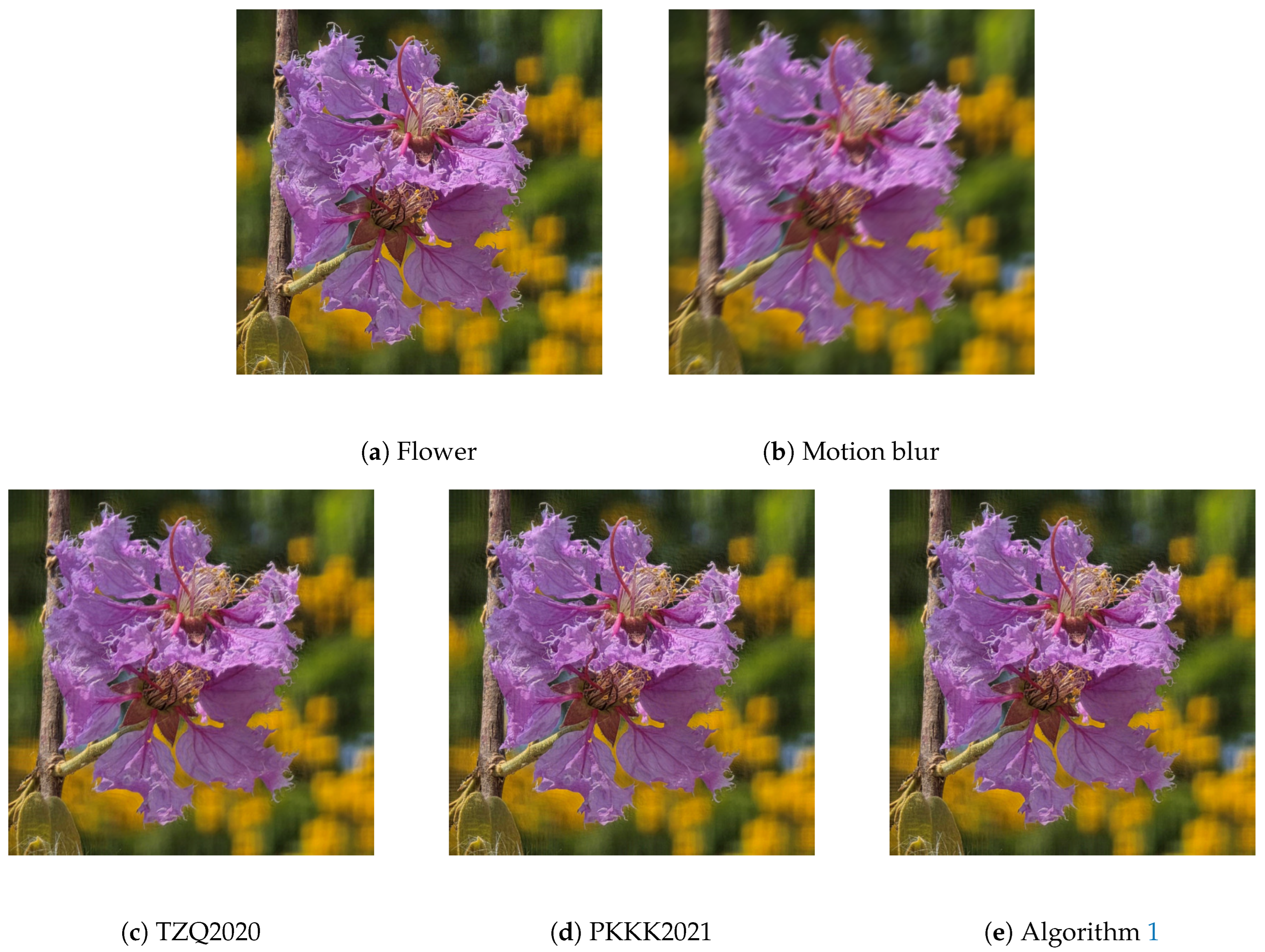
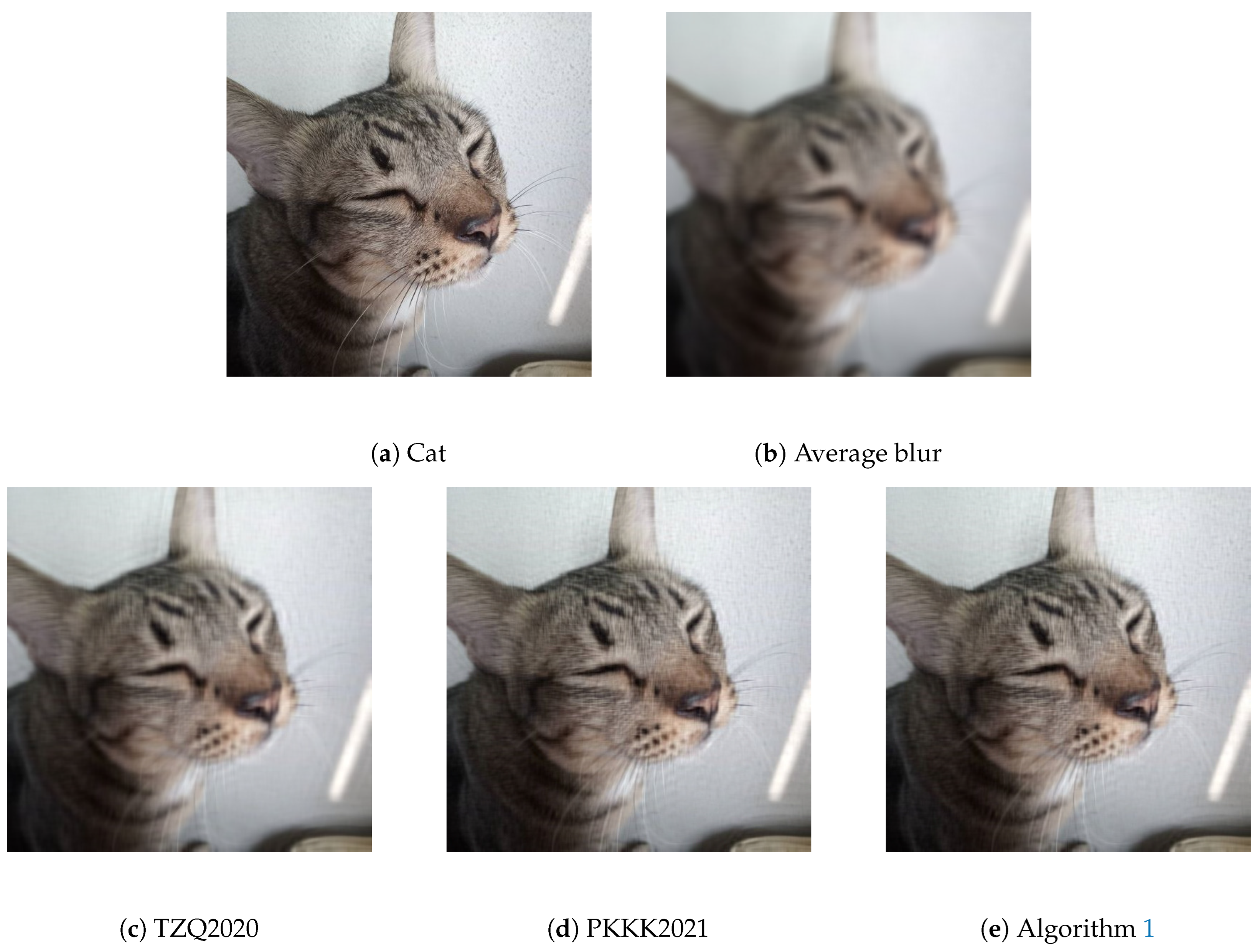
For the numerical experiments, two test images (a flower image and a cat image) captured by the authors using a personal digital camera were used. These images were selected to demonstrate the performance of the proposed algorithm for image restoration under different types of blur and noise. The degraded images were generated by applying blur operators and additive noise, and the restoration performance was evaluated using standard image quality metrics such as ISNR and SSIM. All the experiments were implemented in MATLAB R2019a running on a personal computer with an Intel(R) Core(TM) i7-7700HQ CPU @ 2.80 GHz processor and 20 GB of RAM, running a 64-bit operating system.
Image restoration aims to remove blur artifacts and enhance the quality of degraded images, and has been extensively studied in the literature [28,29,30]. Mathematically, the objective of image restoration is to recover the original image v from a degraded observation u. A commonly used mathematical model describing the relationship between v R n × 1 and u R m × 1 is given by
u = Π v + ε ,
where Π R m × n represents the blur operator, and ε R m × 1 denotes the additive noise. The reconstructed image can be obtained by solving the following LASSO (Least Absolute Shrinkage and Selection Operator) problem:
find v arg min v R n × 1 1 2 Π v u 2 2 + λ v 1 .
where λ > 0 is a penalty parameter, · 1 denotes the l 1 -norm, and · 2 denotes the standard Euclidean norm.
Let h 1 : R n × 1 R be defined by h 1 ( v ) = 1 2 Π v u 2 2 , and let h 2 : R n × 1 R be defined by h 2 ( v ) = λ v 1 . Solving Equation (29) is equivalent to solving a monotone inclusion problem. In particular, the problem corresponds to an image restoration model when we set P as the gradient of h 1 , that is, P : = h 1 , and Q as the subdifferential of h 2 , that is, Q : = h 2 . Hence, the problem can be written as follows:
find v R n × 1 such that 0 ( P + Q ) v ,
where
P = h 1 = 1 2 Π ( · ) u 2 2 = Π T ( Π ( · ) u ) ,
where Π is the transpose of Π and
Q = h 2 v = p H h 2 ( a ) h 2 ( v ) + p , a v , a H .
To quantify the quality of the reconstructed image, we gauge it using the improvement in signal-to-noise ratio (ISNR) for images, which is defined as follows:
ISNR ( n ) = 10 log 10 v u 2 2 v v n 2 2 ,
where v, u and v n represent the original image, degraded image and the restored image at iteration n, respectively. In addition, we also employ the structural similarity index measure (SSIM) [31] to assess the perceptual quality of the reconstructed images. The test images are original photographs taken by the authors and do not belong to any publicly available dataset. The following table summarizes the parameter configurations for each algorithm.
Table 1. Parameter settings of the algorithms.
AlgorithmParameters
θ ¯ ε n ω n φ n
TZQ2020 0.9000 1000 n 2 0.5 150 n 1000 n + 100
PKKK2021 0.9000 1000 n 2 0.5 150 n 1000 n + 100
Proposed (Algorithm 1) 0.9000 1000 n 2 0.5 150 n 1000 n + 100 0.999 ( 0.899 ) 2 n
Table 2. Experimental settings for image restoration tests.
Image/SettingImage SizeType of BlurNoise LevelRegularization Parameter
Flower 512 × 512 Motion ( l = 9 , θ = 40 ) N U ( 0 , σ ) 512 × 512 λ = 0.001
Cat 512 × 512 Average ( 15 × 15 ) N U ( 0 , σ ) 512 × 512 λ = 0.001
Here, θ denotes the motion direction in degrees measured counter-clockwise. The noise is modeled as N U ( 0 , σ ) m × n , where σ controls the noise level. In this study, σ = 0.001 . The notation U ( 0 , σ ) represents the uniform distribution on the interval ( 0 , σ ) , meaning that each entry of N is independently drawn from this distribution.
Figure 1. Comparison of image restoration results for the Flower image. The original image (a) is degraded by motion blur (b). Restoration results obtained by TZQ2020 (c), PKKK2021 (d), and the proposed Algorithm 1 (e) are presented for comparison.
Symmetry 18 00782 g001
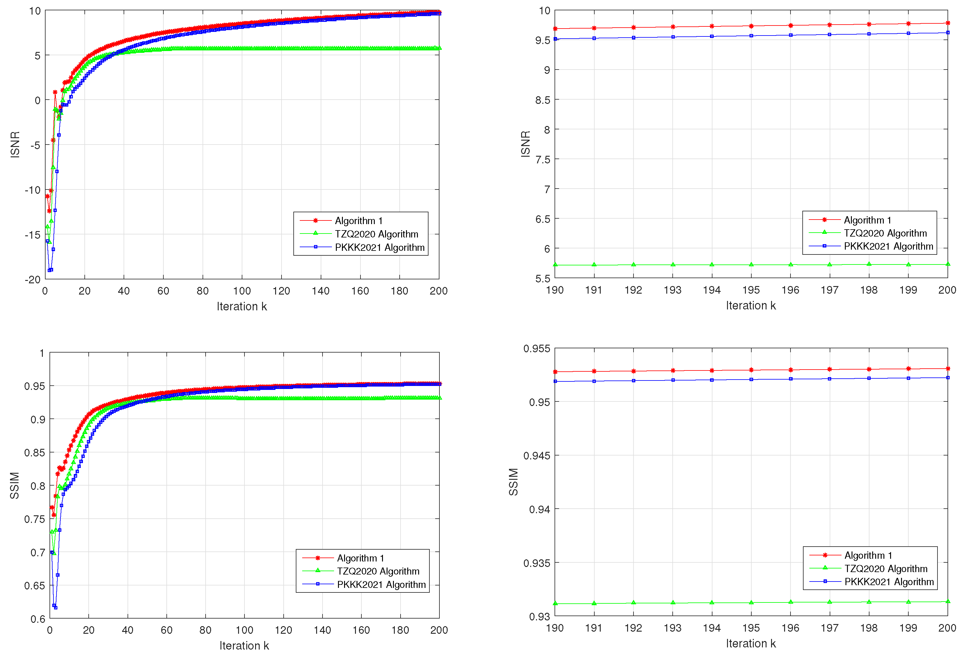
Figure 2. Flower. Quantitative comparison of ISNR and SSIM for different methods under motion blur. The top row shows ISNR curves (full and zoomed views), while the bottom row shows SSIM curves.
Symmetry 18 00782 g002
Figure 3. Comparison of image restoration results for the cat image. The original image (a) is degraded by average blur (b). Restoration results obtained by TZQ2020 (c), PKKK2021 (d), and the proposed Algorithm 1 (e) are presented for comparison.
Symmetry 18 00782 g003
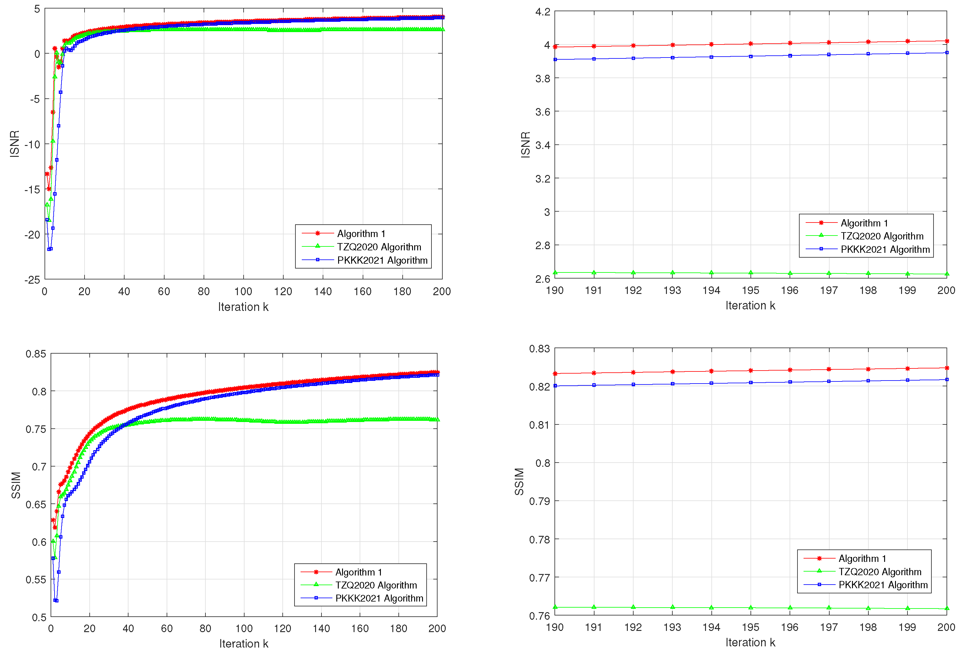
Figure 4. Cat. Quantitative comparison of ISNR and SSIM for different methods under average blur. The top row shows ISNR curves (full and zoomed views), while the bottom row shows SSIM curves.
Symmetry 18 00782 g004
Table 3. ISNR and SSIM values for the “Flower”image obtained by Algorithm 1, TZQ2020, and PKKK2021 at different iterations.
(k)ISNRSSIM
Algorithm 1 TZQ2020 PKKK2021 Algorithm 1 TZQ2020 PKKK2021
1−10.7700−14.1610−15.74400.76690.72940.6995
101.93310.8802−0.60770.85300.81710.8031
507.07535.44646.29960.93530.92710.9280
1008.48865.69628.14620.94710.94720.9449
2009.77945.72559.63140.95320.93130.9525
Table 4. ISNR and SSIM values for the “Cat”image obtained by Algorithm 1, TZQ2020, and PKKK2021 at different iterations.
(k)ISNRSSIM
Algorithm 1 TZQ2020 PKKK2021 Algorithm 1 TZQ2020 PKKK2021
1 13.3190 16.7810 18.3900 0.6283 0.5998 0.5780
10 1.3875 0.8198 0.2304 0.6983 0.6804 0.6636
50 3.0833 2.5646 2.8072 0.7830 0.7585 0.7691
100 3.5384 2.6064 3.4060 0.8044 0.7606 0.7981
2004.0209 2.6247 3.9507 0.8247 0.7616 0.8218

5. Conclusions

In this paper, we proposed a new inertial forward–backward–forward algorithm (Algorithm 1) combined with a moving point projection technique for solving monotone inclusion problems in real Hilbert spaces. The proposed method integrates the advantages of inertial extrapolation and projection-based techniques, while avoiding the need to compute projections onto the intersection of multiple sets as required in some classical hybrid projection methods. Under suitable assumptions on the operators and control parameters, we established the weak convergence of the sequence generated by Algorithm 1 to a solution of the monotone inclusion problem (3).
To demonstrate the practical performance of the proposed method, numerical experiments were conducted on image restoration problems formulated as LASSO problems (29). The parameter settings and experimental configurations are summarized in Table 1 and Table 2, respectively. The visual restoration results shown in Figure 1 and Figure 3 indicate that Algorithm 1 produces clearer reconstructed images. In addition, the quantitative comparisons reported in Table 3 and Table 4, together with the convergence behavior illustrated in Figure 2 and Figure 4, confirm that the proposed method achieves superior performance in terms of the improvement in signal-to-noise ratio (ISNR) and the structural similarity index measure (SSIM) when compared with the TZQ2020 and PKKK2021 algorithms.
Overall, the proposed algorithm provides an effective and reliable approach for solving monotone inclusion problems and shows strong potential for practical applications in image restoration.

Author Contributions

Conceptualization, V.B., K.U., S.P., R.W. and P.T.; methodology, K.U. and P.T.; software, K.U. and P.T.; validation, V.B., S.P., R.W. and K.U.; convergence analysis, K.U. and P.T.; investigation, K.U. and P.T.; writing—original draft preparation, K.U. and P.T.; writing—review and editing, V.B., K.U., S.P. and P.T.; visualization, K.U. and P.T.; project administration, K.U. and P.T. All authors have read and agreed to the published version of the manuscript.

Funding

This project and Kasamsuk Ungchittrakool were supported by National Research Council of Thailand (NRCT) and Naresuan University. Grant NO. N42A660516. Moreover, this work was partially supported by Frontier Research and Innovation Cluster Fund, Naresuan University; Grant number R2569C008.

Data Availability Statement

The data presented in this study are included in the article. The test images used in the numerical experiments (flower and cat images) were captured by the authors using a personal camera and are available from the corresponding author upon reasonable request.

Acknowledgments

The authors sincerely thank Vasile Berinde for the ERASMUS+ grant awarded to Purit Thammasiri for his three-month research visit at the Faculty of Sciences, Technical University of Cluj-Napoca, North University Centre of Baia Mare, Romania, and this project and Kasamsuk Ungchittrakool were supported by National Research Council of Thailand (NRCT) and Naresuan University, Grant NO. N42A660516, while this work was partially supported by Frontier Research and Innovation Cluster Fund, Naresuan University; Grant number R2569C008.

Conflicts of Interest

The authors declare no conflicts of interest.

References

  1. Berinde, V. Approximating Fixed Points of Lipschitzian Pseudocontractions; Mathematics & Mathematics Education (Bethlehem, 2000); World Sci. Publishing: River Edge, NJ, USA, 2002. [Google Scholar]
  2. Berinde, V. Iterative Approximation of Fixed Points, 2nd ed.; Lecture Notes in Mathematics, 1912; Springer: Berlin/Heidelberg, Germany, 2007. [Google Scholar]
  3. Takahashi, W. Nonlinear Functional Analysis; Yokohama Publishers: Yokohama, Japan, 2000. [Google Scholar]
  4. Takahashi, W. Introduction to Nonlinear and Convex Analysis; Yokohama Publishers: Yokohama, Japan, 2009. [Google Scholar]
  5. Ungchittrakool, K. Existence and convergence of fixed points for a strict pseudo-contraction via an iterative shrinking projection technique. J. Nonlinear Convex Anal. 2014, 15, 693–710. [Google Scholar] [CrossRef]
  6. Lions, P.L.; Mercier, B. Splitting Algorithms for the Sum of Two Nonlinear Operators. Siam J. Numer. Anal. 1979, 16, 964–979. [Google Scholar] [CrossRef]
  7. Passty, G.B. Ergodic convergence to a zero of the sum of monotone operators in Hilbert space. J. Math. Anal. Appl. 1979, 72, 383–390. [Google Scholar] [CrossRef]
  8. Tseng, P. A modified forward-backward splitting method for maximal monotone mappings. Siam J. Control Optim. 2000, 38, 431–446. [Google Scholar] [CrossRef]
  9. Polyak, B.T. Some methods of speeding up the convergence of iterative methods. Zh. Vychisl. Mat. Mat. Fiz. 1964, 4, 1–17. [Google Scholar] [CrossRef]
  10. Nesterov, Y. A method for solving a convex programming problem with convergence rate O(1/K2). Dokl. Math. 1983, 27, 367–372. [Google Scholar]
  11. Alvarez, F.; Attouch, H. An inertial proximal method for maximal monotone operators via discretization of a nonlinear oscillator with damping. Set-Valued Anal. 2001, 9, 3–11. [Google Scholar] [CrossRef]
  12. Alvarez, F. Weak convergence of a relaxed and inertial hybrid projection-proximal point algorithm for maximal monotone operators in Hilbert space. SIAM J. Optim. 2004, 14, 773–782. [Google Scholar] [CrossRef]
  13. Attouch, H.; Bolte, J.; Svaiter, B.F. Convergence of descent methods for semi-algebraic and tame problems: Proximal algorithms, forward-backward splitting, and regularized Gauss-Seidel methods. Math. Program. 2009, 137, 91–129. [Google Scholar] [CrossRef]
  14. Lorenz, D.A.; Pock, T. An inertial forward-backward algorithm for monotone inclusions. J. Math. Imaging Vis. 2015, 51, 311–325. [Google Scholar] [CrossRef]
  15. Petrot, N.; Khonchaliew, M.; Suwannaprapa, M. Modified inertial Tseng type method for zeros of the sum of monotone operators in Hilbert spaces. Carpathian J. Math. 2024, 40, 399–417. [Google Scholar] [CrossRef]
  16. Peng, Z.-Y.; Li, D.; Zhao, Y.; Liang, R.-L. An accelerated subgradient extragradient algorithm for solving bilevel variational inequality problems involving non-Lipschitz operator. Commun. Nonlinear Sci. Numer. Simul. 2023, 127, 107549. [Google Scholar] [CrossRef]
  17. Rattanaseeha, K.; Khonchaliew, M. Modified inertial subgradient extragradient algorithm with self-adaptive step sizes for solving split equilibrium problems. J. Nonlinear Anal. Optim. 2023, 14, 71–85. [Google Scholar]
  18. Bnouhachem, A. An inertial extragradient algorithm for a common solution of generalized mixed equilibrium problem and fixed point problem of nonexpansive mappings. Ann. Univ. Ferrara 2025, 71, 10. [Google Scholar] [CrossRef]
  19. Alansari, M.; Ali, R.; Farid, M. Krasnosel’skiǐ-Mann-type subgradient extragradient algorithms for variational inequality and hierarchical fixed-point problems. Mathematics 2025, 13, 3740. [Google Scholar] [CrossRef]
  20. Peng, Z.-Y.; Jolaoso, L.O.; Shehu, Y.; Yao, J.-C. An extrapolated projection and contraction algorithm with past iterates. Numer. Algorithm 2026. [Google Scholar] [CrossRef]
  21. Padcharoen, A.; Kitkuan, D.; Kumam, W.; Kumam, P. Tseng methods with inertial for solving inclusion problems and application to image deblurring and image recovery problems. Comput. Math. Methods 2020, 3, e1088. [Google Scholar] [CrossRef]
  22. Nakajo, K.; Takahashi, W. Strong convergence theorems for nonexpansive mappings and nonexpansive semigroups. J. Math. Anal. Appl. 2003, 279, 372–379. [Google Scholar] [CrossRef]
  23. Tan, B.; Zhou, Z.; Qin, X. Accelerated projection-based forward-backward splitting algorithms for monotone inclusion problems. J. Appl. Anal. Comput. 2020, 10, 2184–2197. [Google Scholar] [CrossRef] [PubMed]
  24. Ungchittrakool, K.; Plubtieng, S.; Tansee, H.; Thammasiri, P. An inertial forward-backward algorithm with moving point projection method for solving monotone inclusion problems. Bangmod Int. J. Math. Comput. Sci. 2026, 12, 1–20. [Google Scholar] [CrossRef]
  25. Brézis, H.; Chapitre, I.I. Operateurs maximaux monotones. North-Holl. Math. Stud. 1973, 5, 19–51. [Google Scholar]
  26. Opial, Z. Weak convergence of the sequence of successive approximations for nonexpansive mappings. Bull. Am. Math. Soc. 1967, 73, 591–597. [Google Scholar] [CrossRef]
  27. Thammasiri, P.; Wangkeeree, R.; Ungchittrakool, K. A modified inertial Tseng’s algorithm with adaptive parameters for solving monotone inclusion problems with efficient applications to image deblurring problems. J. Comput. Anal. Appl. 2024, 33, 782–797. [Google Scholar]
  28. Muangchoo, K.; Phiangsungnoen, S. Hybrid CG-like algorithm for nonlinear equations and image restoration. Carpathian J. Math. 2025, 41, 171–191. [Google Scholar] [CrossRef]
  29. Wangkeeree, R.; Wangkeeree, R.; Belay, Y.A.; Ungchittrakool, K.; Thammasiri, P.; Preechasilp, P. A Halpern method for solving perturbed double inertial Krasnoselskii–Mann iterations with applications to image restoration problems. Bangmod Int. J. Math. Comput. Sci. 2025, 11, 358–360. [Google Scholar] [CrossRef]
  30. Rehman, H.u.; Peng, Z.-Y.; Yao, J.-C. Approximate subgradient extragradient methods for solving variational inequality problems: Convergence analysis and applications in signal and image processing. Commun. Nonlinear Sci. Numer. Simul. 2026, 152, 109211. [Google Scholar] [CrossRef]
  31. Wang, Z.; Bovik, A.C.; Sheikh, H.R.; Simoncelli, E.P. Image quality assessment: From error visibility to structural similarity. IEEE Trans. Image Process. 2004, 13, 600–612. [Google Scholar] [CrossRef]
Disclaimer/Publisher’s Note: The statements, opinions and data contained in all publications are solely those of the individual author(s) and contributor(s) and not of MDPI and/or the editor(s). MDPI and/or the editor(s) disclaim responsibility for any injury to people or property resulting from any ideas, methods, instructions or products referred to in the content.