Variance Analysis of Initial Elasticity Modulus and Bulk Modulus Parameters of Duncan–Chang E-B Model

Abstract

The stress and deformation sensitivity analysis of high earth-rock dams requires knowledge of the statistical mean and standard deviation of deformation parameters of dam materials. However, these parameters are typically determined through grouped tests and sorting. Given the small sample size in each group and the consequently large parameter errors, the inaccuracy of the resulting statistical parameters is evident. The least squares method fits all test points of each group in the same coordinate system for regression calculation, which not only helps to better address the issue of a small sample size, but also eliminates the errors caused by the grouping of test parameters. However, it is found that when the least squares method is applied to the elastic modulus and bulk modulus parameters of the Duncan–Chang E-B model, the residual errors have heteroscedasticity and correlation, which violates the use condition of the least squares method. In order to eliminate the heteroscedasticity and correlation of the fitting residuals of the elastic modulus and bulk modulus parameters of the Duncan–Chang E-B model, this paper decomposes the covariance matrix of the regression residuals to obtain its square root matrix, multiplies the explanatory variables, dependent variables and residual vectors of the regression equation by the square root matrix of the covariance, respectively, and performs variable substitution. The new regression equation has the homogeneity of variance and the irrelevance of the residual. The mean and variance of the model parameters are obtained directly by calculating all the experimental data. The variance of the new parameters is smaller than that of the classical least squares method. The results demonstrate that this generalized least squares method improves the estimation accuracy of elastic modulus and bulk modulus parameters of the Duncan–Chang E-B model.

1. Introduction

Deformation control of the dam body is the most critical technical challenge in high earth-rock dam construction, and stress-deformation prediction during the design stage serves as its foundation. Numerical calculations, despite their current accuracy limitations, have become the primary basis for foundation treatment, material zoning, and deformation control. A reliable prediction requires not only an appropriate constitutive model but also accurate statistical characterization of its deformation parameters. Among existing high core-wall dams, some have experienced surface cracks at the dam top and the upstream slope [1,2]; in high concrete-faced rock dams, phenomena such as disengagement or fracture of the concrete face slab and crushing of vertical joints have occurred. Historically, there have also been cases of core-wall earth-rock dams collapsing due to hydraulic fracturing [3]. All these issues are attributed to inadequate control of dam body deformation [4].

Currently, as the height of dams increases, the design and safety assessment of high earth-rockfill dams increasingly rely on finite element calculations. As specified in the design codes for rolled earth-rockfill dams, namely SL274-2020 [5], detailed requirements are provided for the analysis of stresses and deformations within the dam body. After computations, the numerical results must be analyzed to determine the development and extent of plastic zones, tensile stress zones, cracks, and hydraulic fracturing within the dam. Additionally, the stresses and deformations at the interfaces between the impervious element and the abutments, as well as other structures and connections, must be examined to assess the potential for seepage failure in the impervious element and its interfaces with the abutments and other structural connections. In engineering practice, due to the ambiguity of the concept of the plastic zone, when using the elastoplastic model for calculation, plastic zones may exist everywhere within the dam body. Therefore, in the revision of another book with the same title and the current regulations, NB/T10872-2021 [6], the emphasis on qualitative analysis of factors such as the plastic zone is no longer emphasized. However, the requirements for the stress and deformation analysis of high earth-rock dams have not been reduced; instead, it is required to focus on analyzing settlement, differential settlement, and whether there is cracking, etc. If the calculated post-construction settlement at the dam crest exceeds 1% of the dam height, the reasonableness of the selected fill material compaction criteria and the necessity of implementing engineering measures should be demonstrated based on the analysis of computational results. Therefore, the reliability of finite element calculation results for high earth-rockfill dams directly influences the engineering scheme and safety of the project [7,8,9].

The reliability of numerical stress-deformation analysis for high earth-rockfill dams hinges on whether the selected soil constitutive model and its parameters accurately reflect the actual engineering mechanical properties of the coarse-grained soil materials for dam construction. For numerical simulations of earth and rockfill dams, the Duncan–Chang hyperbolic constitutive model—a nonlinear elastic formulation—has gained widespread acceptance in geotechnical practice. For determining model parameters, the common practice involves collecting bulk samples from the field, transporting them to the laboratory, and reconstituting specimens for testing. However, since the maximum particle size of gravel and rockfill materials is often large, testing usually requires using materials with reduced particle sizes. The general rule is that the maximum particle size used in tests should not exceed one-fifth of the diameter of the triaxial sample, leading to a size effect. Generally speaking, the cost of large triaxial tests is high, the duration is long, and the number of material test groups are limited. The test materials for dam construction cannot cover the gradation variations encountered in the field, nor can they encompass the fluctuations in the on-site filling density. Therefore, a certain number of experiments are usually conducted, and at the same time, engineering analogies are combined to comprehensively determine the numerical calculation parameters [10,11,12].

To better control the deformation of high earth-rock dams, it is often necessary to conduct a sensitivity analysis of the dam deformation based on varying deformation parameters during the design process. The sensitivity analysis of deformation should be carried out in combination with the engineering characteristics, the test results for the dam materials, and the engineering experience, to determine the combination of deformation parameters. The deformation sensitivity analysis of high earth-rock dams requires a clear understanding of the statistical characteristics of each deformation parameter, namely its mean and variance, in order to determine the sensitivity analysis plan. However, due to the limited number of test series for each fill material, determining the mean and variance of deformation parameters is challenging. Even for extra-high earth-rockfill dams, where 11 sets of deformation parameter tests may be conducted for each material, each group of tests consists of six confining pressures. This is because the cost of large-scale triaxial tests is high, and the test period is long, coupled with the fact that each mega-project requires the study of a wide variety of dam-building materials. The current practice is that the sensitivity analysis schemes for the dam body are typically established using combinations of the mean value, small-value average, and large-value average of the deformation parameters. In this context, the small-value average denotes the arithmetic mean of observations falling below the overall mean, whereas the large-value average represents the arithmetic mean of observations exceeding the overall mean. Consequently, these three metrics—small-value average, overall mean, and large-value average—approximate the first quartile (25th percentile), median (50th percentile), and third quartile (75th percentile) of the stress-deformation parameter distribution, respectively [13,14,15].

However, current engineering practice determines deformation parameters through grouped tests with small sample sizes (four to six confining pressures per group), and then uses the mean, small-value average, and large-value average for sensitivity analysis—a crude approximation that ignores parameter uncertainty.

Table 1. Parameters for Stress-Deformation Sensitivity Analysis of a High Core Rockfill Dam.

Earth Material	Scheme 1	Scheme 2	Scheme 3	Scheme 4	Scheme 5
Rockfill I	Mean Value	Small-Value Average	Mean Value	Large-Value Average	Mean Value
Rockfill II					Minimum Value
Core Soil	Mean Value	Small-Value Average	Small-Value Average	Small-Value Average	Mean Value

presents such a computational scheme for a high core rockfill dam, which is evidently relatively crude. A more scientific approach involves determining the variance of the deformation parameters to enable parameter combinations at any percentile among different fill materials, followed by finite element calculations to assess dam safety. Furthermore, with the advancement in design standards, probability distribution and reliability analysis of dam deformation has become imperative, requiring knowledge of the mean and variance of deformation parameters [16,17,18,19]. When ordinary least squares (OLS) are applied to fit the initial elastic modulus and bulk modulus parameters of the Duncan–Chang E-B model, the residuals exhibit heteroscedasticity and correlation across confining pressures, violating the Gauss–Markov assumptions. This study therefore proposes a generalized least squares (GLS) method to eliminate these residual violations and directly obtain the mean and variance of the deformation parameters from all test data, thereby improving estimation accuracy for subsequent reliability analysis.

2. The Duncan–Chang E-B Model and Its Parameter Determination Method

Based on the synthesis of previous experimental stress–strain curves for soils, Kondner postulated that the relationship between deviatoric stress and axial strain could be described by a hyperbolic function [20,21,22].

$${\sigma }_1-{\sigma }_3={\displaystyle \frac{{\epsilon }_a}{a+b{\epsilon }_a}}$$

where ${\sigma }_1-{\sigma }_3$ is the deviatoric stress (difference between the major and minor principal stresses ${\sigma }_1$,${\sigma }_3$); ${\epsilon }_a$ is the axial strain; $a,b$ are intermediate variables; $a=1/E_i,b=1/{({\sigma }_1-{\sigma }_3)}_{ult}$. $E_i$ is the initial tangent modulus of the stress–strain curve; ${({\sigma }_1-{\sigma }_3)}_{ult}$ is the asymptotic value of the deviatoric stress when the strain is large enough [20].

Based on this premise, the tangent modulus formula for the Duncan–Chang E-B model was derived as follows:

$$E_t=E_i{(1-R_{f}S)}^2$$

where $R_f={({\sigma }_1-{\sigma }_3)}_f/{({\sigma }_1-{\sigma }_3)}_{ult}$ is the failure ratio; the stress level is $S=(1-\sin \phi )({\sigma }_1-{\sigma }_3)/(2c\cos \phi +2{\sigma }_3\sin \phi )$. And the cohesion and friction angle of the dam rockfill materials are $c=0,\phi ={\phi }_0-\Delta \phi \lg ({\sigma }_3/P_a)$; the reference atmospheric pressure is $P_a$, equal to 101.325 kPa; the initial elastic modulus is $E_i$, and the bulk modulus $B$ is expressed as follows:

$$E_i=K{P}_a{({\sigma }_3/P_a)}^n,B=K_b{P}_a{({\sigma }_3/P_a)}^m$$

(1)

where $K$ and $n$ are the modulus coefficient and exponent, respectively; $K_b$ and $m$ are the bulk modulus coefficient and exponent, respectively.

Table 2. Classification of Parameters for the Duncan–Chang E-B Model.

Parameter Category	Tangent Modulus Parameters	Bulk Modulus Parameters	Strength Parameters	Failure Ratio
Parameters	$K,n$	$K_b,m$	$c,\phi$ or ${\phi }_0,\Delta \phi$	$R_f$

lists the classification of parameters for the Duncan–Chang E-B model. Parameter $K,n$, governing the initial elastic modulus, and parameter $K_b,m$, governing the bulk modulus (or Poisson’s ratio), are the most critical deformation parameters. For determining parameter $K,n$, the code recommends using the line connecting the data points at 70% and 95% stress levels as the basis for calculating the initial tangent modulus, $E_i$, under each confining pressure [23]. When determining parameter $K_b,m$, the code suggests selecting the peak point on the volumetric strain curve for $B_i=({\sigma }_1-{\sigma }_3)/3{\epsilon }_V$. $({\sigma }_1-{\sigma }_3)$ and ${\epsilon }_V$ are the principal stress differences corresponding to the peak stress point and its volume strain value. If the volumetric strain curve does not exhibit a peak before the principal stress difference reaching 70% of the peak strength, then the point $0.7{({\sigma }_1-{\sigma }_3)}_f$ and its corresponding volumetric strain should be used.

The code further stipulates that each set of tests should include four to six confining pressure levels. Each experimental series, encompassing consolidated drained triaxial compression tests conducted at four to six distinct confining stress levels, generates a unique parameter set characterizing the Duncan–Chang E–B constitutive behavior. If 11 sets of tests are conducted, 11 values for each parameter listed in Table 2 can be compiled, allowing for the calculation of the mean, small-value average, and large-value average of each parameter. However, due to the limited sample size—with only four to six data points available for fitting parameters such as $K,n$, and $K_b,m$—the parameter errors are significant, and the inaccuracy of the resulting statistical parameters is self-evident.

The determination of $K,n$ and $K_b,m$ essentially involves fitting experimental data points. By applying the least squares method to fit all sample points from each test group, the mean values of parameters $K,n$ and $K_b,m$ can be directly obtained. This approach not only effectively addresses the issue of small sample size, but also eliminates the inherent errors contained in the parameters $K,n$ and $K_b,m$ derived from individual test groups. Subsequently, the variance or standard deviation of the parameters can be calculated based on all sample points, thereby enabling the determination of parameter values at any desired percentile.

3. Classical Least Squares Method for Linear Fitting [24,25]

Assuming that Y is the dependent variable, X is the independent variable influencing Y, and they are assumed to exhibit a linear relationship, as follows:

$$Y={\beta }_0+{\beta }_{1}X+e$$

(2)

where e is the residual term, representing the combined effects of factors other than X on Y, as well as experimental measurement errors, etc., ${\beta }_0,{\beta }_1$ are the unknown parameters to be estimated. Given n sets of observed values $(x_i,y_i),i=1,2,\dots ,n$, then:

$$y_i={\beta }_0+{\beta }_1{x}_i+e_i,i=1,2,3,\dots ,n$$

(3)

If the residual term $e_i,i=1,2,\dots ,n$ satisfies the Gauss–Markov assumptions, namely: (a) $E(e_i)=0$; (b) $Var(e_i)={\sigma }^2$, $i=1,2,\dots ,n$ (constant variance); and (c) $Cov(e_i,e_j)=0$, $i\ne j$ (no correlation), then the least squares estimators are valid. The matrix form of the aforementioned equation can be obtained:

$$y=X\beta +e,E(e)=0,Cov(e)={\sigma }^{2}I$$

(4)

A fundamental technique for estimating the parameter vector $\beta$ is the least squares method. It aims to find an estimate of $\beta$ such that the squared length (i.e., the sum of squares) of the residual vector $e=y-X\beta$, expressed as ${‖y-X\beta ‖}^2$, is minimized. In other words:

$$Q(\beta )={‖y-X\beta ‖}^2=(y-X\beta {)}^{\prime }(y-X\beta )$$

where $(y-X\beta {)}^{\prime }$ is the transpose of matrix $(y-X\beta )$. Expanding this equation can be given as follows:

$$Q(\beta )=y^{\prime }y-2y^{\prime }X\beta +{\beta }^{\prime }{X}^{\prime }X\beta$$

Taking the partial derivatives with respect to $\beta$ and setting them to zero, the normal equations can be obtained:

$$X^{\prime }X\beta =X^{\prime }y$$

(5)

The solution for parameter $\beta$ is given as

$$\beta =(X^{\prime }X{)}^{-1}{X}^{\prime }y$$

Substituting the n sets of observed data $(x_i,y_i)$ into the above equation yields an estimated value of the parameter as $\widehat{\beta }$.

$$\widehat{\beta }={(X^{\prime }X)}^{-1}{X}^{\prime }y$$

(6)

The covariance matrix of the parameter $\widehat{\beta }$ can be expressed as

$$Cov(\widehat{\beta })={\sigma }^2{(X^{\prime }X)}^{-1}$$

(7)

4. Test for Homoscedasticity and Non-Correlation of Residuals in the Duncan–Chang E-B Model Parameter Fitting Equations

All data used in this paper were obtained from actual large-scale triaxial tests conducted in the laboratory. The test program was sufficiently extensive, and the results met expectations. The presented mean and variance of deformation parameters for each dam construction material provide a basis for probabilistic calculations of deformation in high earth-rockfill dams.

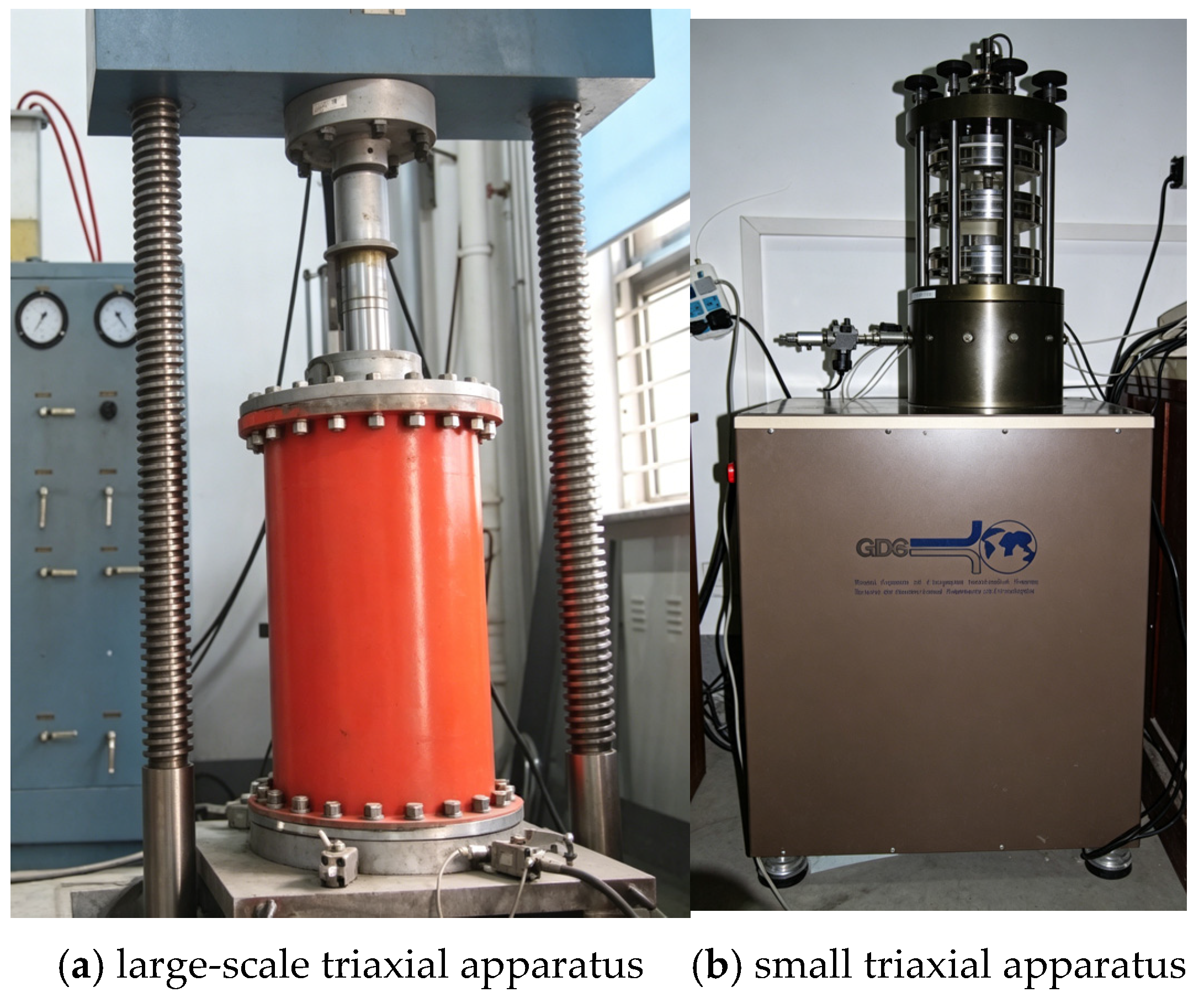
The equipment used for the stress–strain curve test of the dam construction materials is shown in Figure 1. Large triaxial consolidation drained (CD) tests were conducted on the Zone I granite rockfill material. Meanwhile, small triaxial consolidation drained (CD) tests were performed on the gravelly clay and sand. The sample diameter for the large-scale triaxial test was 300 mm, and the height was 600 mm. The small triaxial apparatus can conduct triaxial tests with two different diameters. For the sand, tests had a sample diameter of 61.8 mm and a height of 150 mm. For the gravelly clay triaxial test, the sample diameter was 100 mm, and the height was 200 mm.

4.1. Goodness-of-Fit Test for Initial Elastic Modulus Parameters K and n

Dividing both sides of the first expression in Equation (1) by $P_a$ and taking the logarithm yields the following [20]:

$$\log (E_i/P_a)=\lg (K)+n\lg ({\sigma }_3/P_a)$$

(8)

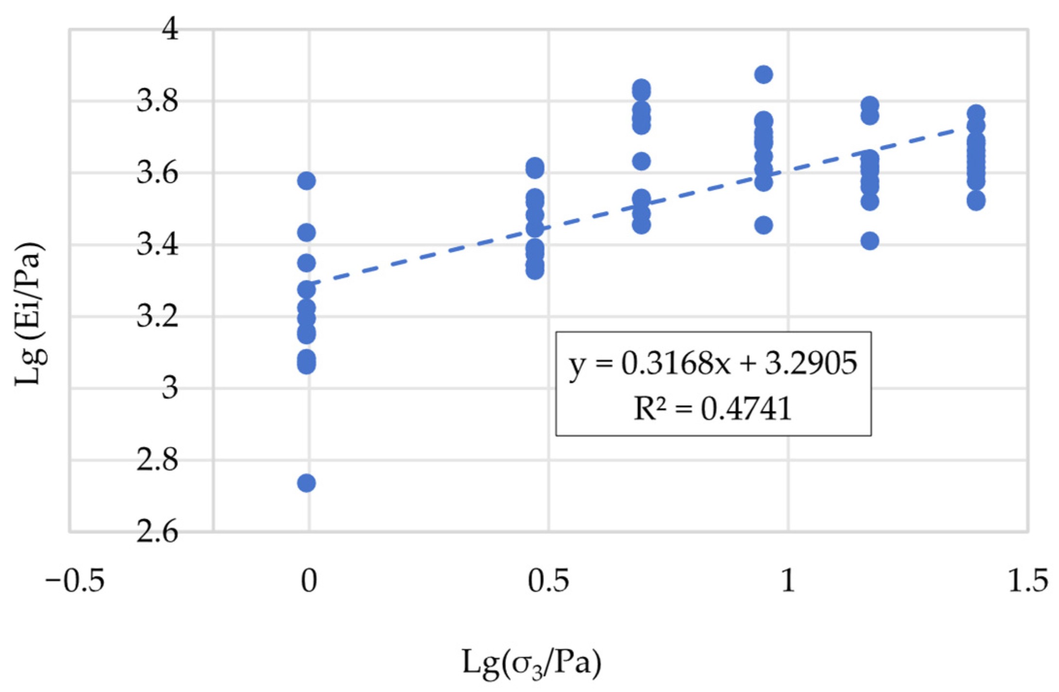
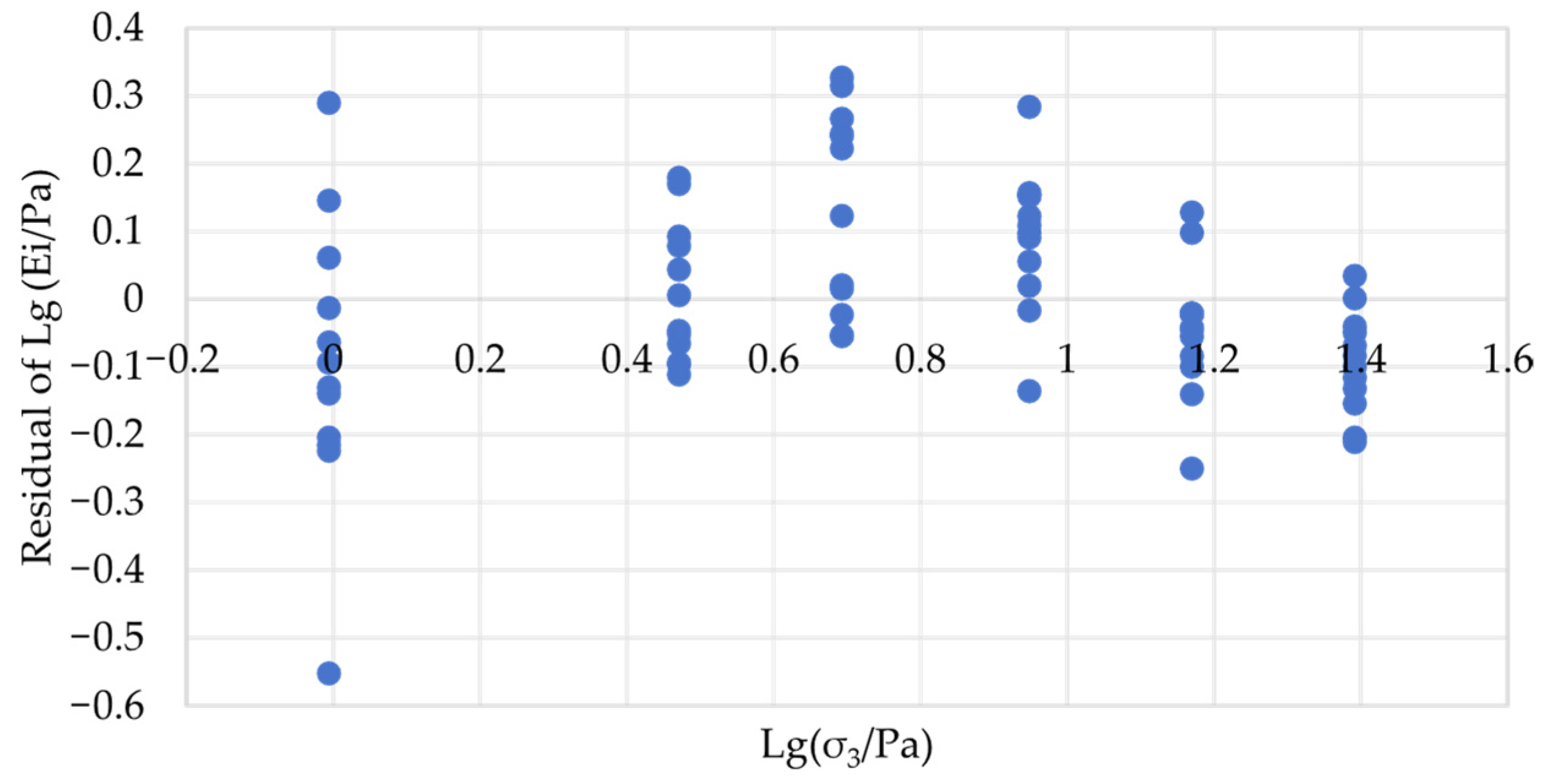
Twelve sets of tests were conducted on the Zone I granite rockfill material from a high dam, and the initial elastic modulus parameters of K and n were fitted, as presented in Figure 2. Figure 3 shows the corresponding residual plot. It can be observed from the figure that the residuals exhibit an inconsistent distribution across different confining pressures.

The coefficient of determination (R² = 0.4741) for this global fitting is relatively low, indicating considerable scatter in the measured initial elastic modulus of the rockfill material. Such scatter is common in practical engineering due to variations in gradation, compaction density, and testing errors. The conventional grouped-test approach would produce 12 separate parameter sets with even greater uncertainty. The low R² actually underscores the necessity of studying the variance of the elastic modulus parameters. By directly providing the mean equation and the variance of the parameters, the proposed GLS method enables deformation predictions at different probability levels, which is more informative for engineering design.

Whether the regression residuals of the elastic modulus satisfy homoscedasticity and non-correlation must be verified through hypothesis testing. The specific procedure is as follows: first, the Kolmogorov–Smirnov (K-S) test is used to examine whether the residuals at each confining pressure conform to a normal distribution; then, based on the fact that the ratio of sample variances of the regression residuals across different confining pressures follows an F-distribution, a test is conducted to determine whether the residual variances at various confining pressures are consistent at a certain probability level (quantile), i.e., a homoscedasticity test; finally, the serial correlation among regression disturbances across varying confinement levels is examined via hypothesis testing.

For the 12 test sets on Zone I granite rockfill material of the high dam, the residuals of the elastic modulus regression $\lg (E_i/P_a)$ under each confining pressure and their variances are presented in

Table 3. Residuals and Residual Variances from the Least Squares Regression of the Elastic Modulus.

The Confining Pressure (kPa)	$\mathbf{Residual} \mathbf{of} \mathbf{lg}({\mathit{E}}_{\mathit{i}}/{\mathit{P}}_{\mathit{a}})/\times {10}^{-2}$												Variance
100	−1.33	−55.26	−6.4	−20.48	−13.06	28.94	14.53	6.07	−21.55	−9.41	−13.96	−22.41	4.48
300	0.55	−6.59	4.33	−11.17	−9.5	−9.58	−5.18	17.88	−4.71	9.21	7.85	16.97	1.06
500	−5.5	−5.36	22.24	24.33	2.01	31.46	32.68	−2.33	12.27	24.1	1.51	26.59	2.19
900	1.92	−13.61	15.15	15.63	28.38	12.22	9.73	9.07	5.54	10.87	−1.69	15.34	1.09
1500	−14.06	−5.54	9.78	−10.02	−4.44	−25.05	12.75	−2.11	−2.26	−8.42	−4.22	−2.16	0.98
2500	−8.4	−6.93	−15.45	−11.61	−9.99	−21.09	−20.46	−4.96	3.42	0.1	−13.23	−4.06	0.57

.

4.1.1. K-S Test for Normality of Regression Residuals

(1)

Null and alternative hypotheses $H_0:F\left(x\right)=F_0(x),H_1:F\left(x\right)\ne F_0(x)$, where $F_0(x)$ is the hypothesized normal distribution function.

(2)

Selection of the test statistic: Using $D_n=\sup \left|F_n(x)-F(x)\right|$ as the pivot, where $F_n\left(x\right)$ is the sample distribution function, sup$\left|\dots \right|$ is the maximum vertical distance between the cumulative distribution functions. When the null hypothesis is true, the test statistic follows distribution $D_n=\sup \left|F_n(x)-F_0(x)\right|$. At a significance level $\alpha$, a reasonable test is to reject the null hypothesis if $\sqrt{n}{D}_n>k$, where $k$ is an appropriate constant, and n is the sample size. Kolmogorov derived the limiting distribution of $\sqrt{n}{D}_n$ and tabulated it for reference.

(3)

Determination of the rejection region: Given the significance level $\alpha$, such that $P(\sqrt{n}{D}_n\ge t_{\alpha })=\alpha$, look up the quantile $t_{\alpha }$ as the critical value. The rejection region is then defined as $\left[t_{\alpha },\infty \right)$.

If a significance level of $\alpha =0.05$ is given, satisfying condition $P(\sqrt{n}{D}_n\ge t_{0.05})=0.05$, the tabulated value $t=1.22$ is used as an approximation for $t_{0.05}$, resulting in the rejection region $\left[1.22,+\infty \right)$. The computational results of the normality test for the regression residuals under each confining pressure are presented in

Table 4. Normality Test of Regression Residuals Under Various Confining Pressures.

Confining Pressure/kPa	Mean of Residuals	Standard Deviation of Residuals	${\mathit{d}}_{01}$	${\mathit{d}}_{02}$	$\sqrt{\mathit{n}}{\mathit{D}}_{\mathit{n}}$	$\mathbf{Falls} \mathbf{into} \mathbf{Rejection} \mathbf{Region} \left[1.22,+\mathit{\infty }\right)$	Normal Distribution
100	−0.095	0.212	0.1876	0.1071	0.65	No	Accept
300	0.0084	0.1029	0.1221	0.2054	0.71	No	Accept
500	0.1367	0.1481	0.219	0.2019	0.759	No	Accept
900	0.0905	0.1044	0.1667	0.181	0.609	No	Accept
1500	−0.0465	0.0990	0.1474	0.2307	0.776	No	Accept
2500	−0.0939	0.0754	0.06287	0.0959	0.323	No	Accept

. It can be concluded that the regression residuals $\lg (E_i/P_a)$ at each confining pressure follow normal distribution.

4.1.2. Test for Homoscedasticity of Regression Residuals Under Various Confining Pressures

Theoretical studies indicate that the F-test is particularly sensitive to deviations from homoscedasticity; therefore, it is employed to examine the variances of residuals across different confining pressures. The null hypothesis (H₀) and alternative hypothesis are as follows: $H_0:{\sigma }_1^2={\sigma }_2^2=\dots ={\sigma }_k^2$, $H_1:{\sigma }_1^2,{\sigma }_2^2,\dots ,{\sigma }_k^2$ not all equal.

(1)

The test statistic of the F-distribution

According to the variance test theory of the bivariate normal distribution population, the ratio of the sample variance of residuals under two confining pressures to the overall variance follows an F distribution, i.e.,

$${\displaystyle \frac{S_1^2/{\sigma }_1^2}{S_2^2/{\sigma }_2^2}}\sim F\left(n_1-1,n_2-1\right)$$

where $S_1^2$ and $S_2^2$ are the variances of the sample regression residuals under two compressive pressures, ${\sigma }_1^2$ and ${\sigma }_2^2$ are the overall variances of the regression residuals, and $n_1$ and $n_2$ are the sample sizes.

If the null hypothesis holds, that is, the variances of the regression residuals under the two confining pressures are equal, then the statistic is

$$F=S_1^2/S_2^2$$

It follows an F distribution with degrees of freedom $\left(n_1-1,n_2-1\right)$.

(2)

Determination of the rejection region

Take $\alpha =0.05$ such that

$$P(F\le F_{1-\frac{\alpha }{2}}(n_1-1,n_2-1))={\displaystyle \frac{\alpha }{2}}, P(F\ge F_{\frac{\alpha }{2}}(n_1-1,n_2-1))={\displaystyle \frac{\alpha }{2}}$$

(9)

$$P({\displaystyle \frac{S_1^2}{S_2^2}}\le F_{0.975}(11,11))=0.025$$

$$F_{0.975}(11,11)={\displaystyle \frac{1}{F_{0.025}(11,11)}}={\displaystyle \frac{1}{3.48}}=0.287356$$

$$F_{0.025}(11,11)=3.48$$

Then, the rejection region is defined by $\left(0,0.2874\right]$ and $\left[3.48,+\infty \right)$.

(3)

Test for homoscedasticity of regression residuals

Table 5. Variance Ratios of Least Squares Regression Residuals Under Different Confining Pressures.

Confining Pressure/kPa	100	300	500	900	1500	2500
100	1/$\surd$	0.2359/$\times$	0.489/$\surd$	0.2432/$\times$	0.2186/$\times$	0.1268/$\times$
300	0.2359/$\times$	1/$\surd$	2.0725/$\surd$	1.0308/$\surd$	0.9267/$\surd$	0.5372/$\surd$
500	0.489/$\surd$	2.0725/$\surd$	1/$\surd$	0.4974/$\surd$	0.4471/$\surd$	0.2592/$\times$
900	0.2432/$\times$	1.0308/$\surd$	0.4974/$\surd$	1/$\surd$	0.899/$\surd$	0.5212/$\surd$
1500	0.2186/$\times$	0.9267/$\surd$	0.4471/$\surd$	0.899/$\surd$	1/$\surd$	0.5798/$\surd$
2500	0.1268/$\times$	0.5372/$\surd$	0.2592/$\times$	0.5212/$\surd$	0.5798/$\surd$	1/$\surd$

Note: √ means the null hypothesis is not rejected; × means rejection.

lists the variance ratios of the regression residuals under each confining pressure and indicates whether they fall within the rejection region. The symbol “$\surd$” indicates that the variance ratio lies within the acceptance region, and the null hypothesis can be accepted; the symbol “$\times$” indicates that the variance ratio falls within the rejection region, and the null hypothesis is rejected.

It can be observed that, with the exception of the diagonal entries where the variance ratio of regression residuals at each confining pressure equals 1, 10 instances of the variance ratios fall within the acceptance region, while five instances lie in the rejection region. Therefore, the null hypothesis of homoscedasticity for the residuals of the original regression equation is rejected.

4.1.3. Test for Independence of Elastic Modulus Regression Residuals Under Various Confining Pressures

Assuming the regression residuals under different confining pressures are two distinct random variables, X and Y, the test for independence is equivalent to testing their correlation coefficient $\rho$.

(1)

The null and alternative hypotheses are $H_0:\rho =0,H_1:\rho \ne 0$. The sample correlation coefficient $R$ serves as the point estimator for $\rho$. The calculation of $R$ is according to Equation (10) and presented in

Table 6. Computation of R Values.

Confining Pressure/kPa	100	300	500	900	1500	2500
100	1	-	-	-	-	-
300	0.027	1	-	-	-	-
500	0.424	−0.11	1	-	-	-
900	0.413	−0.053	0.453	1	-	-
1500	−0.14	0.242	0.077	0.077	1	-
2500	−0.54	0.380	−0.029	−0.143	−0.029	1

.

$$R={\displaystyle \frac{{\displaystyle {\sum }_{i=1}^n(X_i-\overline{X})(Y_i-\overline{Y})}}{\sqrt{{\displaystyle {\sum }_{i=1}^n{(X_i-\overline{X})}^2}}\sqrt{{\displaystyle {\sum }_{i=1}^n{(Y_i-\overline{Y})}^2}}}}$$

(10)

(2)

The test statistic of the t-distribution

When the null hypothesis (H₀) is true, it can be shown that the statistic is as follows:

$$t={\displaystyle \frac{R}{\sqrt{1-R^2}}}\sqrt{n-2}$$

(11)

which follows a t-distribution with n − 2 degrees of freedom. The computation of $t$ is presented in

Table 7. Calculation of t-Values.

Confining Pressure/kPa	100	300	500	900	1500	2500
100	-	-	-	-	-	-
300	0.086/$\surd$	-	-	-	-	-
500	1.479/$\surd$	−0.351/$\surd$	-	-	-	-
900	1.433/$\surd$	−0.169/$\surd$	1.605/$\surd$	-	-	-
1500	−0.447/$\surd$	0.79/$\surd$	0.243/$\surd$	0.243/$\surd$	-	-
2500	−2.031/$\times$	1.3/$\surd$	−0.091/$\surd$	−0.455/$\surd$	−0.091/$\surd$	-

Note: √ means the null hypothesis is not rejected; × means rejection.

.

Determine the rejection region.

Given a significance level $\alpha$, such that

$$P\left(\left|t\right|\ge t_{\frac{\alpha }{2}}(n-2)\right)=\alpha$$

(12)

If the observed value of $t$ satisfies condition $\left|t\right|\ge t_{\frac{\alpha }{2}}(n-2)$, then the null hypothesis $H_0$ is rejected. Given $\alpha =0.1$, $P(\left|t\right|\ge t_{0.05}(10))=0.05$, and $t_{0.05}(10)=1.8125$, the rejection region is defined as the union of $\left(-\infty ,-1.8125\right]$ and $\left[1.8125,+\infty \right)$.

(3)

Test for independence of regression residuals

As can be seen from Table 7, one of the aforementioned t-values lies within the rejection region; therefore, the hypothesis of residual independence across confining pressures is rejected.

The above analysis demonstrates that when fitting the initial elastic modulus parameters $K,n$ of the Duncan–Chang E-B model for rockfill material, the residuals exhibit both heteroscedasticity and correlation, thereby violating the Gauss–Markov assumptions. Since satisfaction of the Gauss–Markov assumptions is a prerequisite for linear regression using the least squares method, it is imperative to seek an enhancement of this method to overcome the heteroscedasticity and correlation in the fitting residuals [24,25].

4.2. Goodness-of-Fit Test for Parameters $K_b,m$

Dividing both sides of the second expression in Equation (1) by $P_a$ and taking the logarithm yields the following:

$$\lg (B/P_a)=\lg (K_b)+m\lg ({\sigma }_3/P_a)$$

(13)

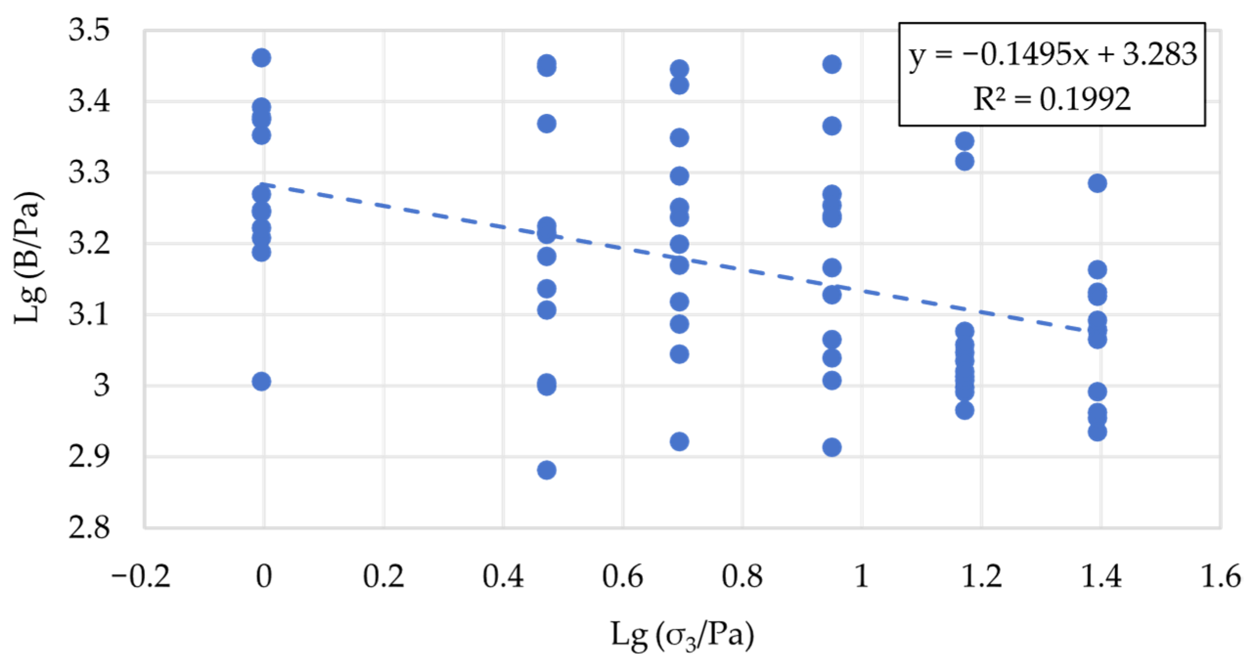
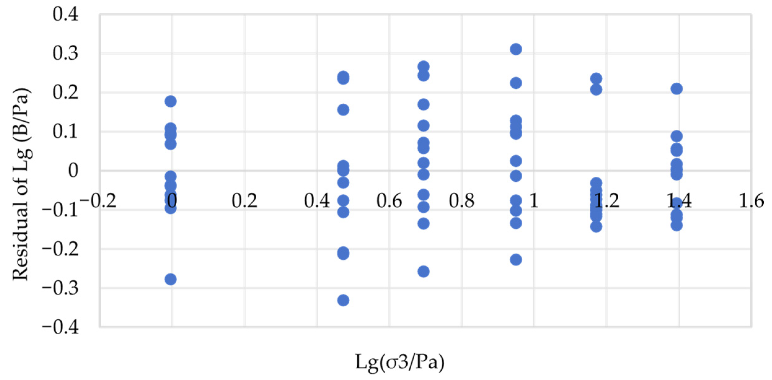
The bulk modulus values obtained from 12 triaxial tests on Zone I rockfill material from a specific project were fitted using the least squares method, as shown in Figure 4. The residuals from the fitted bulk modulus are presented in Figure 5.

For the 12 triaxial tests on Zone I rockfill material, the residuals of the least squares regression for the bulk modulus $\lg (B/P_a)$ under each confining pressure and their variances are listed in

Table 8. Residuals and Residual Variances from the Least Squares Regression of the Bulk Modulus.

Confining Pressure/kPa	$\mathbf{Residual} \mathbf{of} \mathbf{lg}(\mathit{B}/{\mathit{P}}_{\mathit{a}})$												Variance
100	−0.037	−0.2775	−0.0395	−0.0145	0.0688	−0.0757	0.0909	0.1778	−0.0615	0.1084	0.0942	−0.0956	0.0136
300	0.0006	−0.3311	−0.0303	−0.2085	−0.076	0.0124	0.1564	0.2356	0.0036	−0.2129	−0.1058	0.2406	0.0288
500	−0.0096	−0.1348	0.0718	0.0202	−0.0611	−0.2575	0.2439	0.1158	0.0578	0.1699	−0.0925	0.2666	0.0222
900	−0.0131	−0.0761	0.0948	0.1283	0.1129	−0.2275	0.3114	0.2246	−0.1019	0.0252	−0.1335	0.0981	0.0221
1500	−0.0949	−0.0314	−0.0614	−0.1103	−0.1165	−0.1424	0.2361	0.2079	−0.0728	−0.1008	−0.0878	−0.0502	0.0141
2500	0.0039	0.0034	−0.1394	−0.12	0.0568	0.0173	−0.1122	0.2101	0.0512	−0.0093	−0.083	0.0887	0.0093

.

4.2.1. K-S Test for Normality of Bulk Modulus Regression Residuals

Normality Test of Bulk Modulus Regression Residuals Under Each Confining Pressure

Given a significance level of $\alpha =0.05$, let $P(\sqrt{n}{D}_n\ge t_{0.05})=0.05$ and $t=1.22$ serve as approximate values for $t_{0.05}$; then, the rejection region is $\left[1.22,+\infty \right)$. The computational results are presented in

Table 9. Normality Test for Regression Residuals of $\lg (B/P_a)$ Under Various Confining Pressures.

Confining Pressure/kPa	Mean of Residuals	Standard Deviation of Residuals	${\mathit{d}}_{01}$	${\mathit{d}}_{02}$	${\mathit{n}}^{0.5}{\mathit{D}}_{\mathit{n}}$	$\mathbf{Falls} \mathbf{into} \mathbf{Rejection} \mathbf{Region} \left[1.22,+\mathit{\infty }\right)$	Normal Distribution
100	−0.0051	0.1168	0.11707	0.1265	0.5308	No	Accept
300	−0.0268	0.1699	0.1090	0.1599	0.5541	No	Accept
500	0.0325	0.1489	0.0889	0.0686	0.3078	No	Accept
900	0.0369	0.1487	0.1513	0.1097	0.5241	No	Accept
1500	−0.0354	0.1188	0.2366	0.3200	1.1084	No	Accept
2500	−0.0027	0.0964	0.1394	0.1310	0.4829	No	Accept

.

Therefore, it can be concluded that the regression residuals of $\lg (B/P_a)$ under various confining pressures follow normal distribution.

4.2.2. Test for Homoscedasticity of Bulk Modulus Regression Residuals Under Various Confining Pressures

As with the elastic modulus, the F-test is employed to assess homoscedasticity. The null and alternative hypotheses are as follows: $H_0:{\sigma }_1^2={\sigma }_2^2=\dots ={\sigma }_k^2$, $H_1:{\sigma }_1^2,{\sigma }_2^2,\dots ,{\sigma }_k^2$ not all equal.

Given a confidence level $\alpha =0.05$, if conditions $P\left(F\le F_{1-\alpha /2}(n_1-1,n_2-1)\right)=\alpha /2$ and $P\left(F\ge F_{\alpha /2}(n_1-1,n_2-1)\right)=\alpha /2$ satisfied, then the rejection region comprises both $\left(0,0.2874\right]$ and $\left[3.48,+\infty \right)$.

Table 10. Variance Ratios of Least Squares Regression Bulk Modulus Residuals Under Different Confining Pressures.

Confining Pressure/kPa	100	300	500	900	1500	2500
100	1/$\surd$	0.4730/$\surd$	0.6155/$\surd$	0.6168/$\surd$	0.9661/$\surd$	1.4685/$\surd$
300	0.4730/$\surd$	1/$\surd$	1.3013/$\surd$	1.3039/$\surd$	2.0424/$\surd$	3.1045/$\surd$
500	0.6155/$\surd$	1.3013/$\surd$	1/$\surd$	1.0020/$\surd$	1.5695/$\surd$	2.3858/$\surd$
900	0.6168/$\surd$	1.3039/$\surd$	1.0020/$\surd$	1/$\surd$	1.5664/$\surd$	2.3809/$\surd$
1500	0.9661/$\surd$	2.0424/$\surd$	1.5695/$\surd$	1.5664/$\surd$	1/$\surd$	1.5200/$\surd$
2500	1.4685/$\surd$	3.1045/$\surd$	2.3858/$\surd$	2.3809/$\surd$	1.5200/$\surd$	1/$\surd$

Note: √ means the null hypothesis is not rejected.

lists the variance ratios of the bulk modulus regression residuals under each confining pressure and indicates whether they fall within the rejection region. A check mark (√) indicates that the variance ratio lies within the acceptance region and the null hypothesis can be accepted; a cross symbol (×) signifies that the F-statistic ratio lies in the critical region, leading to the rejection of the null hypothesis. As can be seen from Table 10, the variance homoscedasticity for the bulk modulus regression residual $\lg (B/P_a)$ is accepted.

4.2.3. Test for Independence of Bulk Modulus Regression Residuals Under Various Confining Pressures

Similarly to Section 4.1.3, the independence test is equivalent to testing the correlation coefficient $\rho$ of the bulk modulus regression residuals under different confining pressures. The null and alternative hypotheses are $H_0:\rho =0,H_1:\rho \ne 0$. The sample correlation coefficient $R$ is used as the point estimator for $\rho$. The computed values of E are given in

Table 11. Correlation Coefficients of Least Squares Regression Bulk Modulus Residuals Under Different Confining Pressures.

Confining Pressure/kPa	100	300	500	900	1500	2500
100	1	-	-	-	-	-
300	0.3704	1	-	-	-	-
500	0.3611	0.5056	1	-	-	-
900	0.4727	0.4271	0.7375	1	-	-
1500	0.3923	0.5594	0.5238	0.7096	1	-
2500	0.1133	0.4450	0.0574	0.0080	0.2060	1

, and the t-values are provided in

Table 12. The t-Values of the Least Squares Regression Bulk Modulus Residuals Under Different Confining Pressures.

Confining Pressure/kPa	100	300	500	900	1500	2500
100	-	-	-	-	-	-
300	1.2612/$\surd$	-	-	-	-	-
500	1.2247/$\surd$	1.8533/$\surd$	-	-	-	-
900	1.6961/$\surd$	1.4938/$\surd$	3.4531/$\times$	-	-	-
1500	1.3486/$\surd$	2.1342/$\surd$	1.9444/$\surd$	3.1847/$\times$	-	-
2500	0.3604/$\surd$	1.5712/$\surd$	0.1820/$\surd$	0.0252/$\surd$	0.6657/$\surd$	-

Note: √ means the null hypothesis is not rejected; × means rejection.

.

If the observed t-value satisfies condition $\left|t\right|\ge t_{\frac{\alpha }{2}}(n-2)$, the null hypothesis is rejected. Taking $\alpha =0.05$, $P(\left|t\right|\ge t_{0.025}(10))=0.025$, and $t_{0.025}(10)=2.2281$, the rejection region is defined as the union of $\left(-\infty ,-2.2281\right]$ and $\left[2.2281,+\infty \right)$.

It can be observed that two of the aforementioned t-values fall within the rejection region. Although 13 values lie in the acceptance region, the null hypothesis is nevertheless rejected. Consequently, when fitting the bulk modulus parameters K_b and m of the Duncan–Chang E-B model for rockfill, the residual vectors are considered to be correlated and not independent, despite the presence of homoscedasticity. This violates the Gauss–Markov assumptions and therefore fails to satisfy the application conditions of the least squares method [24,25].

5. Generalized Least Squares Method for Eliminating Residual Heteroscedasticity and Correlation [24,25]

If the covariance matrix of the residuals can be obtained as

$$Cov(e)={\sigma }^{2}V$$

(14)

Then the linear regression equation possesses the following property:

$$y=X\beta +e, E(e)=0, Cov(e)={\sigma }^{2}V$$

(15)

where $V$ is nonsingular and positive definite, and there exists a nonsingular symmetric matrix $K$ such that $K^{\prime }K=K^{-1}K=V$. The matrix $K$ is the square root matrix of $V$.

Define new variables as follows:

$$z=K^{-1}y, B=K^{-1}X, g=K^{-1}e$$

(16)

Then, the regression equation $y=X\beta +\epsilon$ is transformed into $K^{-1}y=K^{-1}X\beta +K^{-1}e$, namely:

$$z=B\beta +g$$

(17)

After this transformation, the error term of the model possesses a zero mean, i.e., $E(g)=K^{-1}E(e)=0$. Furthermore, the covariance matrix of $g$ is

$$\begin{gathered} Var(g)=\left\{\left.\left[g-E(g)\right]{\left[g-E(g)\right]}^{\prime }\right\}\right.=E(g{g}^{\prime }) \\ =E(K^{-1}e{e}^{\prime }{K}^{-1})=K^{-1}E(e{e}^{\prime })K^{-1} \\ ={\sigma }^2{K}^{-1}V{K}^{-1}={\sigma }^2{K}^{-1}KK{K}^{-1} \\ ={\sigma }^{2}I \end{gathered}$$

Therefore, the elements of g possess the properties of zero mean, constant variance, and being uncorrelated. Hence, Equation (12) satisfies the general assumptions of the classical least squares estimation. The least squares function can be obtained:

$$Q(\beta )=g^{\prime }g=e^{\prime }{V}^{-1}e=(y-X\beta {)}^{\prime }{V}^{-1}(y-X\beta )$$

The normal equation for the least squares can be expressed as

$$X^{\prime }{V}^{-1}X{\widehat{\beta }}^{*}=X^{\prime }{V}^{-1}y$$

The solution to this equation can be expressed as

$${\widehat{\beta }}^{*}={(X^{\prime }{V}^{-1}X)}^{-1}{X}^{\prime }{V}^{-1}y$$

(18)

Since

$$E({\widehat{\beta }}^{*})=E\left[{(X^{\prime }{V}^{-1}X)}^{-1}{X}^{\prime }{V}^{-1}y\right]={(X^{\prime }{V}^{-1}X)}^{-1}{X}^{\prime }{V}^{-1}X\beta =\beta$$

Therefore, ${\widehat{\beta }}^{*}$ is the generalized least squares estimate of $\beta$.

The covariance of ${\widehat{\beta }}^{*}$ can be expressed as

$$\begin{gathered} Var({\widehat{\beta }}^{*})=Var\left({(X^{\prime }{V}^{-1}X)}^{-1}{X}^{\prime }{V}^{-1}y\right)={(X^{\prime }{V}^{-1}X)}^{-1}{X}^{\prime }{V}^{-1}{\sigma }^{2}V{V}^{-1}{X}^{\prime }{(X^{\prime }{V}^{-1}X)}^{-1} \\ ={\sigma }^2{(X^{\prime }{V}^{-1}X)}^{-1} \end{gathered}$$

(19)

6. Calculation of Duncan–Chang E-B Model Parameters Using the Generalized Least Squares Method

6.1. Elastic Modulus Coefficient and Exponent of the Duncan–Chang E-B Model [26,27]

$$\lg (E_i/P_a)=\lg (K)+n\lg ({\sigma }_3/P_a)$$

Let $\lg (K)={\beta }_0$, $n={\beta }_1$, $\lg (E_i/P_a)=y$, and $\lg ({\sigma }_3/P_a)=x$, then $y={\beta }_0+{\beta }_{1}x$.

By applying the Taylor expansion to $y={\beta }_0+{\beta }_{1}x$, and in accordance with the variance theory in probability theory, we can obtain

$${\sigma }_K^2={(\mathsf{\partial }K/\mathsf{\partial }{\beta }_0)}^2{\sigma }_{{\beta }_0}^2, {\sigma }_n^2={\sigma }_{{\beta }_1}^2,$$

$$Cov(K,n)={\displaystyle \frac{\mathsf{\partial }K}{\mathsf{\partial }{\beta }_0}}{\displaystyle \frac{\mathsf{\partial }n}{\mathsf{\partial }{\beta }_0}}{\sigma }_{{\beta }_0}^2+{\displaystyle \frac{\mathsf{\partial }K}{\mathsf{\partial }{\beta }_1}}{\displaystyle \frac{\mathsf{\partial }n}{\mathsf{\partial }{\beta }_1}}{\sigma }_{{\beta }_1}^2+{\displaystyle \frac{\mathsf{\partial }K}{\mathsf{\partial }{\beta }_0}}{\displaystyle \frac{\mathsf{\partial }n}{\mathsf{\partial }{\beta }_1}}Cov({\beta }_0,{\beta }_1)={\displaystyle \frac{\mathsf{\partial }K}{\mathsf{\partial }{\beta }_0}}Cov({\beta }_0,{\beta }_1)$$

$${\displaystyle \frac{\mathsf{\partial }K}{\mathsf{\partial }{\beta }_0}}={10}^{{\beta }_0}\ln 10$$

where ${\sigma }_K^2,{\sigma }_n^2$ are the variance of the initial shear modulus coefficient and exponent of the Duncan–Chang E-B model, and $Cov(K,n)$ is the covariance of K and n.

The generalized least squares method was applied to the initial elastic modulus obtained from triaxial tests on six groups of sand, 12 groups of gravelly clay core material, and 12 groups of Zone I granite rockfill material. The resulting regression parameters ${\beta }_0$ and ${\beta }_1$ are presented in

Table 13. Regression Parameters and Variances for Initial Modulus.

Material	Least Squares Method	${\mathit{\beta }}_0$	${\mathit{\beta }}_1$	$\mathbf{Variance} \mathbf{of} {\mathit{\beta }}_0$	$\mathbf{Variance} \mathbf{of} {\mathit{\beta }}_1$	$\mathbf{Covariance} \mathbf{Between} {\mathit{\beta }}_0$$\mathbf{and}{\mathit{\beta }}_1$	Heteroscedasticity of Residuals	Correlation of Residuals
Sand	Classical	2.690	0.4656	0.0423	0.0671	−0.0255	Exists	Exists
	Generalized	2.656	0.4864	0.0392	0.0656	−0.0236	Eliminate	Eliminate
Gravelly Clay Core Material	Classical	2.6196	0.4999	0.0236	0.0242	−0.0223	Exists	Exists
	Generalized	2.6594	0.4700	0.0105	0.0114	−0.0097	Eliminate	Eliminate
Zone I Granite Rockfill Material	Classical	3.291	0.317	0.028	0.024	−0.025	Exists	Exists
	Generalized	3.374	0.184	0.015	0.011	−0.012	Eliminate	Eliminate

, while the mean, variance, standard deviation, and coefficient of variation for the initial elastic modulus coefficient and exponent are summarized in

Table 14. Mean, Variance, and Standard Deviation of Initial Modulus Parameters K and n.

Material	Least Squares Method	K	n	Variance of K	Variance of n	Covariance between K and n	Standard Deviation of K	Standard Deviation of n	Coefficient of Variation of K	Coefficient of Variation of n
Sand	Classical	489.9	0.4656	53,833	0.067	−28.73	232.0	0.259	0.4736	0.5565
	Generalized	452.8	0.4864	42,651	0.066	−24.60	206.5	0.257	0.4560	0.5281
Gravelly Clay Core Material	Classical	416.5	0.50	21,701	0.024	−21.368	147.312	0.1557	0.3537	0.3114
	Generalized	456.5	0.47	11,557	0.011	−10.695	107.503	0.1066	0.2355	0.2267
Zone I Granite Rockfill Material	Classical	1952	0.32	573,403	0.0249	−114.2	757	0.158	0.3879	0.4983
	Generalized	2365	0.18	455,435	0.0106	−65.6	675	0.103	0.2854	0.5594

.

It can be observed from the table that, in the regression of the initial elastic modulus, the generalized least squares method not only reduces the variance of the regression parameters ${\beta }_0$ and ${\beta }_1$ compared to the classical least squares method, but also further decreases the standard deviation of the elastic modulus coefficient and exponent in the Duncan–Chang E-B model, thereby enhancing the precision of the regression parameters.

6.2. Bulk Modulus Coefficient and Exponent of the Duncan–Chang E-B Model

$$\lg (B/P_a)=\lg (K_b)+m\lg ({\sigma }_3/P_a)$$

Let $\lg (K_b)={\beta }_0$, $m={\beta }_1$, $\lg (B/P_a)=y$, and $\lg ({\sigma }_3/P_a)=x$, then $y={\beta }_0+{\beta }_{1}x$.

Performing a Taylor expansion of $y={\beta }_0+{\beta }_{1}x$ and applying the variance theory of probability, we can obtain

$${\sigma }_{K_b}^2={(\mathsf{\partial }{K}_b/\mathsf{\partial }{\beta }_0)}^2{\sigma }_{{\beta }_0}^2, {\sigma }_n^2={\sigma }_{{\beta }_1}^2, Cov(K_b,m)={\displaystyle \frac{\mathsf{\partial }{K}_b}{\mathsf{\partial }{\beta }_0}}Cov({\beta }_0,{\beta }_1)$$

where ${\displaystyle \frac{\mathsf{\partial }{K}_b}{\mathsf{\partial }{\beta }_0}}={10}^{{\beta }_0}\ln 10$.

The generalized least squares method was applied to the bulk modulus data obtained from triaxial tests on six groups of sand, 12 groups of gravelly clay core material, and 12 groups of Zone I granite rockfill material. The resulting regression parameters ${\beta }_0$ and ${\beta }_1$ are listed in

Table 15. Regression Parameters ${\beta }_0$ and ${\beta }_1$ for Bulk Modulus from Sand Tests.

Material	Least Squares Method	${\mathit{\beta }}_0$	${\mathit{\beta }}_1$	$\mathbf{Variance} \mathbf{of} {\mathit{\beta }}_0$	$\mathbf{Variance} \mathbf{of} {\mathit{\beta }}_1$	$\mathbf{Covariance} \mathbf{Between} {\mathit{\beta }}_0$$\mathbf{and}{\mathit{\beta }}_1$	Heteroscedasticity of Residuals	Correlation of Residuals
Sand	Classical	1.9635	1.0942	0.2922	1.176	−0.542749	Exists	Exists
	Generalized	2.21085	0.59205	0.0249	0.074	−0.000147	Eliminate	Eliminate
Gravelly Clay Core Material	Classical	2.5267	0.3417	0.02075	0.04469	−0.024786	Exists	Exists
	Generalized	2.4509	0.3612	0.01681	0.04023	−0.024178	Eliminate	Eliminate
Zone I Granite Rockfill Material	Classical	3.2573	−0.129	0.0273	0.0121	−0.0147	Exists	Exists
	Generalized	3.2491	−0.120	0.0191	0.0114	−0.0125	Eliminate	Eliminate

, while the mean, variance, standard deviation, and coefficient of variation of the bulk modulus coefficient and exponent are summarized in

Table 16. Mean, Variance, and Standard Deviation of Bulk Modulus Parameters K_b and m for Sand.

Material	Classical or Generalized LSM	Kb	m	Variance of Kb	Variance of m	Covariance of Kb-m	Standard Deviation of Kb	Standard Deviation of m	Coefficient of Variation of Kb	Coefficient of Variation of m
Sand	Classical	91.9	1.094	13,095	1.176	−114.899	114.4	1.084	1.245	0.991
	Generalized	162.5	0.592	3488	0.074	−0.0559	59.1	0.272	0.363	0.460
Gravelly Clay Core	Classical	336.3	0.34	12,443	0.045	−19.192	111.548	0.2114	0.3317	0.6186
	Generalized	282.5	0.36	7,111	0.040	−15.724	84.327	0.2006	0.2986	0.5553
Zone I Granite Rockfill	Classical	1808.4	−0.13	472,999	0.0121	−19.192	687.7	0.110	0.380	−0.85
	Generalized	1774.5	−0.12	319,128	0.0114	−15.724	564.9	0.107	0.318	−0.89

.

As can be seen from the table above, for the regression of the bulk modulus, the generalized least squares method is superior to the classical least squares method, not only in reducing the variance of the regression parameters ${\beta }_0$ and ${\beta }_1$, but also in lowering the standard deviation of the bulk modulus coefficient and exponent in the Duncan–Chang E-B model, thereby enhancing the precision of the estimated parameters.

7. Conclusions

The control of dam body deformation is a key technical challenge in the construction of high earth-rock dams. And the prerequisite for deformation control during the design stage is the prediction of dam deformation. Given that the calculated deformation of current high earth-rock dams is generally smaller than the actual measured deformation, the existing core wall dams often exhibit cracks at the dam top and the upstream slope, while concrete-faced rockfill dams frequently encounter disengagement of the slab and the cushioning material, fracture of the concrete face slab, and crushing of the concrete on both sides of the vertical joints. To improve the situation of deformation control for high earth-rock dams, conducting a sensitivity analysis of deformation based on variable parameters is a feasible compromise method. The purpose of the deformation sensitivity analysis of the dam is to study the most dangerous conditions of the stress and deformation through finite element calculations with varying parameters, in order to assess the safety of the dam body and obtain the optimal structural layout. For example, when studying the hydraulic splitting problem of a high core-wall rockfill dam, the rockfill material of the dam shell should adopt relatively hard parameters (such as large-value averages), while the core wall should adopt relatively soft parameters (such as small-value averages) for calculation and analysis. The sensitivity analysis of the dam body is also applied to consider the uncertainty of calculation parameters caused by differences in the gradation curves of the earth-rock materials in actual engineering, fluctuations in compaction density, size effect in indoor scaled tests, and errors in indoor experiments.

At present, the deformation sensitivity analysis of the dam body adopts a simple method to take the mean value, the small-value average, which is the average of the values less than the mean of whole samples, and the large-value average, which is the average of the values larger than the mean of whole samples, as calculation indicators. Based on this, the deformation of the dam body under several parameter combinations is obtained, and the safety of the high earth-rock dam is judged accordingly. However, this approach is clearly insufficiently comprehensive. Future development is focused on the probability analysis of the deformation of the dam body of high earth-rock dams. This clearly requires first studying the mean and variance of the deformation parameters of the dam materials.

This paper proposes a method where all data points from various test groups are combined in a single coordinate system, and the least squares method is applied to directly regress the mean values and variance of the parameters. This approach not only effectively addresses the issue of small sample size but also eliminates errors inherent in the parameters derived from individual test groups. However, calculations reveal that when fitting the initial elastic modulus and bulk modulus parameters of the Duncan–Chang E-B model using the least squares method, the residuals exhibit heteroscedasticity and correlation. This violates the assumptions of the least squares method, introducing defects in parameter estimation.

To eliminate the heteroscedasticity and correlation of residuals during the fitting of the initial elastic modulus and bulk modulus parameters in the Duncan–Chang E-B model, this paper decomposes the covariance matrix of the regression residuals and computes its square root matrix. This matrix, serving as transformation matrix, is pre-multiplied by the explanatory variables, dependent variables, and residual vectors, respectively, to perform variable substitution. The transformed regression equation is compliant with the Gauss–Markov assumptions of homoscedastic and serially uncorrelated disturbances. The generalized least squares (GLS) estimation procedure was implemented on triaxial experimental data encompassing six suites of sandy soils, 12 suites of gravelly clay core materials, and 12 suites of Zone I granite rockfill specimens, enabling direct computation of both the first and second moments (mean and variance) for the constitutive parameters. Relative to conventional ordinary least squares (OLS) estimation, the GLS approach produced reduced variance estimates for both the initial tangent modulus coefficients and exponent, and the volumetric modulus coefficients and exponent within the Duncan–Chang E-B framework, thereby improving the accuracy and reliability of parameter estimation.

References

- Ji, E.Y.; Chen, S.S. Simulation method and application of crest cracks in high soil core dams. Chin. J. Geotech. Eng. 2020, 42, 997–1004. [Google Scholar]
- Ai, Z.T.; Ma, G.; Zhang, G.; Wang, J.; Huang, Z.; Zhou, W.; Yang, Q. Supervised parameter updating of deformation analyses for rockfill dams using prior knowledge. Comput. Aided Civ. Infrastruct. Eng. 2025, 40, 4583–4606. [Google Scholar] [CrossRef]
- Chakraborty, A.; Dey, A.; Gautam, S.S. Assessing hydraulic fracturing in earthen-rockfill dam core based on extended finite element (XFEM) framework. Can. Geotech. J. 2025, 62, 1–23. [Google Scholar] [CrossRef]
- Mao, J.; Wang, Z.Z.; Yu, X.K.; Liu, Q.H. Analysis on the zoning and initial elastic modulus of main and secondary rock-fill of CFRD deformation. Adv. Mech. Eng. 2011, 52–54, 601–605. [Google Scholar] [CrossRef]
- SL 274-2020; Design Code for Rolled Earth-Rock Fill Dams. Ministry of Water Resources of the People’s Republic of China: Beijing, China, 2020.
- NB/T 10872-2021; Design Code for Rolled Earth-Rock Fill Dams. National Energy Administration of China: Beijing, China, 2021.
- Wang, X.G. Discussion on several problems of high earth-rockfill dams. Chin. J. Geotech. Eng. 2018, 40, 203–222. [Google Scholar]
- Deng, G.; Huangfu, Z.H.; Wu, Y.L.; Zhang, Y.; Chen, H.; Zhang, Y.; Yang, Y. Development and prospect of deformation compatibility control of earth core embankment dams. J. Hydroelectr. Eng. 2020, 39, 1–16. [Google Scholar]
- Pan, S.; Li, T.; Shi, G.; Cui, Z.; Zhang, H.; Yuan, L. The inversion analysis and material parameter optimization of a high earth-rockfill dam during construction periods. Appl. Sci. 2022, 12, 4991. [Google Scholar] [CrossRef]
- Guo, Q.; Huang, H.; Lu, X.; Chen, J.; Zhang, X.; Zhao, Z. A Methodology for Modeling a Multi-Dimensional Joint Distribution of Parameters Based on Small-Sample Data, and Its Application in High Rockfill Dams. Appl. Sci. 2024, 14, 7646. [Google Scholar] [CrossRef]
- Wu, Y.K.; Zhang, B.Y.; Zhang, Z.L.; Yu, Y. Consolidation analysis of Nuozhadu high earth-rockfill dam based on the coupling of seepage and stress-deformation physical state. Int. J. Geomech. 2016, 16, 04015075. [Google Scholar] [CrossRef]
- Wu, Y.K.; Yuan, H.N.; Yu, Y.Z.; Zhang, B.Y.; Zhang, Z.L. Displacement-based back-analysis of the model parameters of the Nuozhadu high earth-rockfill dam. Sci. World J. 2014, 2014, 247096. [Google Scholar] [CrossRef]
- Han, H.M.; Huang, X.X.; Zha, F.S.; Shi, B.; Zhang, X.; Wei, G. Spatiotemporal settlement deformation characteristics analysis of rockfill dam with anti-impact FBG sensing array. Acta Geotech. 2025, 20, 4803–4816. [Google Scholar] [CrossRef]
- Chen, Z.P.; Yin, Y.; Yu, J.W. Internal deformation monitoring for earth-rockfill dam via high-precision flexible pipeline measurements. Autom. Constr. 2022, 136, 104177. [Google Scholar] [CrossRef]
- Qiu, Z.F.; Meng, Q.; Ma, A.J.; Liu, Y. Influence of stone content, relative density, and gradation on shear dilatancy characteristics of rock-soil mixtures. Mar. Georesources Geotechnol. 2025, 43, 2407–2422. [Google Scholar] [CrossRef]
- Jiang, S.H.; Feng, Z.W.; Liu, X.; Jiang, Q.H.; Huang, J.S.; Zhou, C.B. Inference of probability distributions of geotechnical parameters using adaptive Bayesian updating approach. Rock Soil Mech. 2020, 41, 325–335. (In Chinese) [Google Scholar] [CrossRef]
- Wang, P.Y.; Shen, H.; Qin, Y.; Chen, Y.H.; Lei, H.Z. Spatially Variant Slope Reliability Analysis and Updating Based on Convolutional Neural Networks. J. Wuhan Univ. Technol. 2024, 46, 83–89. (In Chinese) [Google Scholar]
- Tian, H.M.; Li, D.Q. Collaborative updating method for stability reliability of spatially variable soil slopes under changing investigation data. Chin. J. Geotech. Eng. 2024, 46, 1613–1621. [Google Scholar]
- Jiang, S.H.; Zhu, G.Y.; Pan, M.; Lin, L. Parameters Statistics and Reliability Updating of Slopes Based on Monitoring Data. J. Disaster Prev. Mitig. Eng. 2023, 43, 324–332. (In Chinese) [Google Scholar] [CrossRef]
- GB/T 50123-2019; Standard for Geotechnical Testing Method. Ministry of Housing and Urban-Rural Development of the People’s Republic of China: Beijing, China, 2019.
- Akhtarpour, A.; Khodaii, A. Experimental study of asphaltic concrete dynamic properties as an impervious core in embankment dams. Constr. Build. Mater. 2013, 41, 319–334. [Google Scholar] [CrossRef]
- Dong, W.X.; Hu, L.M.; Lv, H.; Yu, Y.Z. Comparison between Duncan and Chang’s EB Model and the Generalized Plasticity Model in the analysis of a high earth-rockfill dam. J. Appl. Math. 2013, 2013, 928721. [Google Scholar] [CrossRef]
- Wang, K.; Tang, H.J.; Zhang, J.M.; Wang, R. Development and evaluation of a practical nonlinear elastic constitutive model for rockfill dam deformation simulation based on monitoring results. Acta Geotech. 2024, 19, 3467–3485. [Google Scholar] [CrossRef]
- Wang, S.G.; Chen, M.; Chen, L.P. Linear Statistical Model: Linear Regression and Variance Analysis; China Higher Education Press: Beijing, China, 1999. (In Chinese) [Google Scholar]
- Montgomery, D.C.; Peck, E.A.; Vining, G.G. Introduction to Linear Regression Analysis, 5th ed.; China Machine Press: Beijing, China, 2022. [Google Scholar]
- Ding, S.L.; Pan, J.J.; Zhao, X.D.; Wang, Y.; Wang, L.; Xu, H.; Lu, Y. Data-driven iterative calibration method for prior knowledge of earth-rockfill dam wetting model parameters. J. Rock Mech. Geotech. Eng. 2026, 18, 1621–1632. [Google Scholar] [CrossRef]
- Ran, L.; Li, M.; Sun, Y.; Ding, S.; Yang, J.; Ma, C. A method for determining the displacement monitoring index for rockfill dams considering material uncertainty. Appl. Sci. 2025, 15, 4164. [Google Scholar] [CrossRef]
Figure 1.
Test apparatus used in this study.
Figure 2.
Global fitting of 12 test sets on Zone I granite rockfill from a high dam: determined initial elastic modulus parameters (K = 1952, n = 0.32).
Figure 3.
Residual plot of the fitted initial elastic modulus coefficient and exponent from 12 test sets on Zone I granite rockfill material of a high dam.
Figure 4.
Fitted bulk modulus coefficient and exponent from 12 triaxial tests on Zone I rockfill material of the project (Kb = 1914, m = −0.1495).
Figure 5.
Residuals of the fitted bulk modulus from 12 triaxial tests on Zone I rockfill material of the project.