A Modified-Degenerate Operational Reformulation of W_α,β,ν-Type Exponential, Trigonometric, and Hyperbolic Functions and Their Laplace Transforms

Abstract

We study a modified-degenerate version of the $W_{\alpha ,\beta ,\nu }$-factorial and the associated exponential, trigonometric, and hyperbolic families obtained by replacing the Euler gamma function with the modified-degenerate gamma function ${\Gamma }_{\lambda }^{*}$, where $\lambda \in (0,1)$. A main conclusion of this paper is that this construction does not generate a genuinely new transcendental family. Indeed, since ${\Gamma }_{\lambda }^{*}\left(s\right)=b_{\lambda }^s\Gamma \left(s\right),b_{\lambda }={\displaystyle \frac{\lambda }{\log (1+\lambda )}},$ all modified-degenerate W-functions reduce to exact rescalings of their non-degenerate counterparts. The novelty of the present work is therefore operational rather than structural. We formulate this transport principle explicitly, derive the corresponding modified-degenerate Laplace-transform identities directly in the spectral variable s, establish the induced convolution rule, and obtain first-order asymptotic expansions as $\lambda \to 0^{+}$. We further show that the associated W-derivative is a formal coefficient-shift operator, and conjugate it to the non-degenerate one under the scaling map. As an application, we present a complete Volterra integral-equation example with polynomial memory, including an explicit resolvent representation for the case $m=1$, together with convergence and residual-error checks supporting the numerical illustrations.

1. Introduction

Generalized factorials are a convenient way to organize the coefficients that appear when one repeatedly applies a nonstandard operator. Once such a factorial is fixed, it naturally generates an “exponential” function by a power series, and its even and odd parts give trigonometric and hyperbolic analogues. This viewpoint is common in fractional calculus and in operational methods, where the series coefficients encode iterated fractional integration and differentiation; see, e.g., [1,2,3].

Droghei and Garra [4] introduced the $W_{\alpha ,\beta ,\nu }$-factorial and the related families ${\mathrm{ExpW}}_{\alpha ,\beta ,\nu }$, ${\mathrm{cosW}}_{\alpha ,\beta ,\nu }$, ${\mathrm{sinW}}_{\alpha ,\beta ,\nu }$, ${\mathrm{coshW}}_{\alpha ,\beta ,\nu }$ and ${\mathrm{sinhW}}_{\alpha ,\beta ,\nu }$. Their analytic background is closely tied to the classical literature initiated by Wright on generalized hypergeometric and generalized Bessel functions [5,6] (see also [7,8,9,10,11,12] for related Wright/Fox–Wright type special functions and their Laplace-transform and fractional-calculus setting). These functions can be viewed as deformed versions of the classical exponential, sine/cosine, and hyperbolic sine/cosine. They also fit naturally into operational calculi for variable-coefficient fractional differential equations, where the underlying generalized factorial captures repeated action of fractional operators. From the viewpoint of applications, this is an important point: generalized exponential, trigonometric, and hyperbolic kernels of Wright/Mittag–Leffler type occur in fractional relaxation and oscillation, viscoelastic wave propagation and dissipation with memory, and fractional-order circuit and control models; see, for example, [13,14,15,16,17]. In that sense, the $W_{\alpha ,\beta ,\nu }$ families are not only formal special functions but also candidate response kernels for hereditary models. The examples developed later in this paper remain benchmark mathematical problems, yet they are chosen to mirror these physically meaningful classes.

In a separate line of work, “degenerate” and “modified-degenerate” versions of the gamma function and the Laplace transform have been studied by deforming the usual exponential kernel; see [18,19,20,21,22,23] and the recent Laplace-type variant [24]. Recent applications of degenerate gamma-based special functions to fractional viscoelasticity may also be found in [17]. For $\lambda \in (0,1)$, the modified-degenerate Laplace transform is:

$${\mathcal{L}}_{\lambda }^{*}\left\{f\right\}\left(s\right)={\int }_0^{\infty }{(1+\lambda s)}^{-t/\lambda }f\left(t\right)dt.$$

Related modified Laplace transforms tailored to generalized fractional operators were proposed in [25]. These are especially convenient for applications: these keep the usual convolution theorem and reduce exactly to the classical Laplace transform after the change in variable ${\rho }_{\lambda }\left(s\right)=\log (1+\lambda s)/\lambda$. A similar simplification holds for the modified-degenerate gamma function, which admits the closed form ${\Gamma }_{\lambda }^{*}\left(s\right)=b_{\lambda }^s\Gamma \left(s\right)$ with $b_{\lambda }=\lambda /\log (1+\lambda )$.

Compared with the existing literature, the present paper occupies a deliberately narrow but explicit position. Relative to [4], we do not enlarge the analytic class of W-type functions; instead, we show how that existing class is transported into the modified-degenerate transform setting. Relative to recent papers on degenerate and modified-degenerate Laplace-type transforms [18,19,24], our contribution is likewise not a new transform theory, but a worked operational calculus written directly in the native spectral variable s. Making this positioning explicit is important for assessing the scope and novelty of the manuscript.

The goal of this paper is to merge these two frameworks in a transparent way and to record precisely what is gained—and what is not gained—from the modified-degenerate replacement. We replace the Euler gamma function in the $W_{\alpha ,\beta ,\nu }$-factorial by ${\Gamma }_{\lambda }^{*}$ and obtain a modified-degenerate factorial ${\left[n\right]}_{\alpha ,\beta ,\nu ;\lambda }^{*}!$. Because ${\Gamma }_{\lambda }^{*}\left(s\right)=b_{\lambda }^s\Gamma \left(s\right)$, the resulting construction is found to be an exact transport of the original $W_{\alpha ,\beta ,\nu }$ theory under a simple scaling of the argument. This is made explicit later in Propositions 3 and 4. Accordingly, we do not claim that a genuinely new special function appears here. Instead, the value of the construction is that the corresponding transform pairs, convolution formulas, and model problems can be written directly in the modified-degenerate Laplace variable s, which is the natural variable in applications based on ${\mathcal{L}}_{\lambda }^{*}$.

For ease of reference, we summarize the main outcomes of this paper as follows:

• We define ${\left[n\right]}_{\alpha ,\beta ,\nu ;\lambda }^{*}!$ and introduce the associated series ${\mathrm{ExpW}}^{*}$, ${\mathrm{cosW}}^{*}$, ${\mathrm{sinW}}^{*}$, ${\mathrm{coshW}}^{*}$, and ${\mathrm{sinhW}}^{*}$.
• Using ${\Gamma }_{\lambda }^{*}\left(s\right)=b_{\lambda }^s\Gamma \left(s\right)$, we prove the exact scaling law ${\left[n\right]}_{\alpha ,\beta ,\nu ;\lambda }^{*}!=b_{\lambda }^{n(\alpha +\beta )}{\left[n\right]}_{\alpha ,\beta ,\nu }!$ and deduce that each modified-degenerate W-function is obtained from its non-degenerate counterpart by rescaling the argument. We further quantify the limit $\lambda \to 0^{+}$ by first-order asymptotic expansions.
• We prove that ${\mathcal{L}}_{\lambda }^{*}$ inherits the classical convolution theorem through the change in variable ${\rho }_{\lambda }\left(s\right)=\log (1+\lambda s)/\lambda$, and we derive explicit transform identities for ${\mathrm{ExpW}}^{*}$ and for the trigonometric/hyperbolic families. The formulas are expressed through the factorial-ratio series ${\Psi }_{\alpha ,\beta ,\nu ;\lambda }^{*}\left(z\right)={\sum }_{n\ge 0}{z}^{n}n!/{\left[n\right]}_{\alpha ,\beta ,\nu ;\lambda }^{*}!$.
• We clarify that the associated W-derivative is a formal coefficient-shift operator, conjugated to the corresponding non-degenerate operator under the scaling map, and not an ordinary closed-form differential operator.
• We include a complete worked Volterra example with polynomial memory, including an explicit inversion for the case $m=1$, and we expand the numerical discussion with convergence and residual checks.

This paper is organized as follows: Section 2 recalls the basic definitions and tools. Section 3 introduces the modified-degenerate $W_{\alpha ,\beta ,\nu }$-factorial. Section 4 defines the induced exponential, trigonometric, and hyperbolic families and records their basic properties. Section 5 discusses the limit $\lambda \to 0^{+}$. Section 6 derives the modified-degenerate Laplace-transform formulas, and Section 7 presents operational and convolution-based applications. In particular, we now make explicit how the generalized oscillator and Volterra-memory examples connect to prototype models from viscoelasticity, wave propagation with memory, and fractional-order engineering systems. Our aim is not to claim a fully calibrated device-specific model, but to show that the modified-degenerate formalism fits analytical structures that are standard in physics and engineering.

2. Preliminaries

This section recalls the $W_{\alpha ,\beta ,\nu }$ factorial and its exponential/trigonometric families from [4], and records the basic properties of the modified-degenerate gamma function that we use later.

Let $\alpha ,\beta \in (0,1)$ and $\nu >0$. The generalized factorial introduced in [4] is:

$${\left[n\right]}_{\alpha ,\beta ,\nu }!={\displaystyle \prod _{i=1}^n}{\displaystyle \frac{\Gamma (\beta i+1)}{\Gamma (\beta i+1-\alpha )}}·{\displaystyle \frac{\Gamma (\beta n+1-\alpha +\nu )}{\Gamma (1-\alpha +\nu )}},n\in \mathbb{N},$$

(1)

with ${\left[0\right]}_{\alpha ,\beta ,\nu }!=1$. The associated exponential function is:

$${\mathrm{ExpW}}_{\alpha ,\beta ,\nu }\left(z\right)={\displaystyle \sum _{n=0}^{\infty }}{\displaystyle \frac{z^n}{{\left[n\right]}_{\alpha ,\beta ,\nu }!}}.$$

(2)

The generalized trigonometric and hyperbolic functions are defined by the even/odd parts:

$$\begin{array}{cccc}\hfill {\mathrm{cosW}}_{\alpha ,\beta ,\nu }\left(z\right)& ={\displaystyle \sum _{n=0}^{\infty }}{\displaystyle \frac{{(-1)}^n{z}^{2n}}{{\left[2n\right]}_{\alpha ,\beta ,\nu }!}},\hfill & \hfill {\mathrm{sinW}}_{\alpha ,\beta ,\nu }\left(z\right)& ={\displaystyle \sum _{n=0}^{\infty }}{\displaystyle \frac{{(-1)}^n{z}^{2n+1}}{{[2n+1]}_{\alpha ,\beta ,\nu }!}},\hfill \end{array}$$

(3)

$$\begin{array}{cccc}\hfill {\mathrm{coshW}}_{\alpha ,\beta ,\nu }\left(z\right)& ={\displaystyle \sum _{n=0}^{\infty }}{\displaystyle \frac{z^{2n}}{{\left[2n\right]}_{\alpha ,\beta ,\nu }!}},\hfill & \hfill {\mathrm{sinhW}}_{\alpha ,\beta ,\nu }\left(z\right)& ={\displaystyle \sum _{n=0}^{\infty }}{\displaystyle \frac{z^{2n+1}}{{[2n+1]}_{\alpha ,\beta ,\nu }!}}.\hfill \end{array}$$

(4)

Fix $\lambda \in (0,1)$. The modified-degenerate gamma function [20] is:

$${\Gamma }_{\lambda }^{*}\left(s\right)={\int }_0^{\infty }{(1+\lambda )}^{-t/\lambda }{t}^{s-1}dt,\Re \left(s\right)>0.$$

(5)

We emphasize that (5) uses the modified-degenerate kernel ${(1+\lambda )}^{-t/\lambda }$. This differs from the degenerate gamma kernel ${(1+\lambda t)}^{-1/\lambda }$ considered in [21]. In particular, the constant $b_{\lambda }=\lambda /\log (1+\lambda )$ arises from the present kernel (5), because this kernel is exactly an exponential kernel in disguise.

Because ${(1+\lambda )}^{-t/\lambda }=\exp \left(-\left(\log \right(1+\lambda )/\lambda )t\right)$, the integral in (5) is a rescaled classical gamma integral ([26], Ch. 5). For later use, we set:

$$b_{\lambda }:={\displaystyle \frac{\lambda }{\log (1+\lambda )}}.$$

(6)

Note that $b_{\lambda }>1$ for all $\lambda \in (0,1)$.

Proposition 1.

For every s with $\Re \left(s\right)>0$:

$${\Gamma }_{\lambda }^{*}\left(s\right)=b_{\lambda }^s\Gamma \left(s\right).$$

(7)

Proof. 

Let $a_{\lambda }:=\log (1+\lambda )/\lambda >0$. Then, ${(1+\lambda )}^{-t/\lambda }=e^{-a_{\lambda }t}$ and (5) becomes ${\Gamma }_{\lambda }^{*}\left(s\right)={\int }_0^{\infty }{e}^{-a_{\lambda }t}{t}^{s-1}dt$. With the change in variables $u=a_{\lambda }t$, we get:

$${\Gamma }_{\lambda }^{*}\left(s\right)=a_{\lambda }^{-s}{\int }_0^{\infty }{e}^{-u}{u}^{s-1}du=a_{\lambda }^{-s}\Gamma \left(s\right).$$

Since $a_{\lambda }>0$, we interpret the complex power by the real logarithm, $a_{\lambda }^{-s}:=\exp (-s\log a_{\lambda })$. Because $a_{\lambda }^{-1}=b_{\lambda }>0$, we have:

$$a_{\lambda }^{-s}=\exp (-s\log a_{\lambda })=\exp \left(s\log b_{\lambda }\right)=b_{\lambda }^s,$$

and therefore (7) follows. □

Corollary 1.

For $\Re \left(s\right)>0$, the function ${\Gamma }_{\lambda }^{*}$ satisfies:

$${\Gamma }_{\lambda }^{*}(s+1)=b_{\lambda }s{\Gamma }_{\lambda }^{*}\left(s\right),b_{\lambda }={\displaystyle \frac{\lambda }{\log (1+\lambda )}}.$$

(8)

Proof. 

From (7) and the classical identity $\Gamma (s+1)=s\Gamma \left(s\right)$, we obtain:

$${\Gamma }_{\lambda }^{*}(s+1)=b_{\lambda }^{s+1}\Gamma (s+1)=b_{\lambda }^{s+1}s\Gamma \left(s\right)=\left(b_{\lambda }s\right)b_{\lambda }^s\Gamma \left(s\right)=b_{\lambda }s{\Gamma }_{\lambda }^{*}\left(s\right),$$

which is the stated formula. □

The modified-degenerate Laplace transform [20] is:

$${\mathcal{L}}_{\lambda }^{*}\left\{f\right\}\left(s\right)={\int }_0^{\infty }{(1+\lambda s)}^{-t/\lambda }f\left(t\right)dt,$$

(9)

whenever the integral converges.

Lemma 1.

Assume that $1+\lambda s\notin (-\infty ,0]$ and let

$${\rho }_{\lambda }\left(s\right):={\displaystyle \frac{\log (1+\lambda s)}{\lambda }}$$

(10)

where log is the principal branch. Then:

$${\mathcal{L}}_{\lambda }^{*}\left\{f\right\}\left(s\right)={\int }_0^{\infty }{e}^{-{\rho }_{\lambda }\left(s\right)t}f\left(t\right)dt=\mathcal{L}\left\{f\right\}\left({\rho }_{\lambda }\left(s\right)\right),$$

(11)

where $\mathcal{L}\left\{f\right\}\left(p\right)={\int }_0^{\infty }{e}^{-pt}f\left(t\right)dt$ denotes the classical Laplace transform [27].

Proof. 

Starting from (9), write the kernel using the principal logarithm:

$${(1+\lambda s)}^{-t/\lambda }=\exp \left(-{\displaystyle \frac{t}{\lambda }}\log (1+\lambda s)\right).$$

With ${\rho }_{\lambda }\left(s\right)=\log (1+\lambda s)/\lambda$ as in (10), this is simply ${(1+\lambda s)}^{-t/\lambda }=e^{-{\rho }_{\lambda }\left(s\right)t}$; so, (9) becomes

$${\mathcal{L}}_{\lambda }^{*}\left\{f\right\}\left(s\right)={\int }_0^{\infty }{e}^{-{\rho }_{\lambda }\left(s\right)t}f\left(t\right)dt.$$

Whenever this integral converges (for instance, when $\Re \left({\rho }_{\lambda }\left(s\right)\right)>0$ and f is of exponential order), it is exactly the classical Laplace transform of f evaluated at $p={\rho }_{\lambda }\left(s\right)$, i.e., ${\mathcal{L}}_{\lambda }^{*}\left\{f\right\}\left(s\right)=\mathcal{L}\left\{f\right\}\left({\rho }_{\lambda }\left(s\right)\right)$. □

A basic identity is the transform of monomials [20]. We give a short proof because we will use it several times.

Lemma 2.

For $n\in {\mathbb{N}}_0$ and $\Re \left({\rho }_{\lambda }\left(s\right)\right)>0$,

$${\mathcal{L}}_{\lambda }^{*}\left\{t^n\right\}\left(s\right)={\left({\displaystyle \frac{\lambda }{\log (1+\lambda s)}}\right)}^{n+1}n!.$$

(12)

Proof. 

By Lemma 1,

$${\mathcal{L}}_{\lambda }^{*}\left\{t^n\right\}\left(s\right)={\int }_0^{\infty }{e}^{-{\rho }_{\lambda }\left(s\right)t}{t}^{n}dt={\displaystyle \frac{n!}{{\rho }_{\lambda }{\left(s\right)}^{n+1}}},$$

where the last equality is the standard Laplace integral for monomials [27]. Since ${\rho }_{\lambda }{\left(s\right)}^{-1}=\lambda /\log (1+\lambda s)$, we obtain (12). □

Proposition 2.

Assume that the classical Laplace convolution theorem applies to f and g at the point $p={\rho }_{\lambda }\left(s\right)$. Then.

$${\mathcal{L}}_{\lambda }^{*}\left\{(f\ast g)\left(t\right)\right\}\left(s\right)={\mathcal{L}}_{\lambda }^{*}\left\{f\right\}\left(s\right){\mathcal{L}}_{\lambda }^{*}\left\{g\right\}\left(s\right),(f\ast g)\left(t\right):={\int }_0^{t}f\left(\tau \right)g(t-\tau )d\tau .$$

(13)

Proof. 

By Lemma 1,

$${\mathcal{L}}_{\lambda }^{*}\{f\ast g\}\left(s\right)=\mathcal{L}\{f\ast g\}\left({\rho }_{\lambda }\left(s\right)\right).$$

Applying the classical convolution theorem at $p={\rho }_{\lambda }\left(s\right)$ gives:

$$\mathcal{L}\{f\ast g\}\left({\rho }_{\lambda }\left(s\right)\right)=\mathcal{L}\left\{f\right\}\left({\rho }_{\lambda }\left(s\right)\right)\mathcal{L}\left\{g\right\}\left({\rho }_{\lambda }\left(s\right)\right)={\mathcal{L}}_{\lambda }^{*}\left\{f\right\}\left(s\right){\mathcal{L}}_{\lambda }^{*}\left\{g\right\}\left(s\right),$$

which is exactly (13). □

Remark 1.

The degenerate gamma function and degenerate Laplace transform use the kernels ${(1+\lambda t)}^{-1/\lambda }$ and ${(1+\lambda t)}^{-s/\lambda }$, respectively [21]. We work with the modified versions because Lemma 1 and Proposition 2 show that the entire operational calculus is transported from the classical Laplace transform by the single substitution $p={\rho }_{\lambda }\left(s\right)$. Thus, the modified-degenerate transform is not “new” in a structural sense, but it is operationally convenient when a problem is naturally formulated with the kernel ${(1+\lambda s)}^{-t/\lambda }$ or when one wishes to keep transform tables, convolution formulas, and inversion formulas in the original spectral variable s rather than rewriting every model in terms of ${\rho }_{\lambda }\left(s\right)$.

3. A Modified-Degenerate ${\mathit{W}}_{\mathit{\alpha },\mathit{\beta },\mathit{\nu }}$ Factorial

This section introduces the modified-degenerate $W_{\alpha ,\beta ,\nu }$ factorial by replacing the classical Gamma function with the modified-degenerate Gamma function, and we derive its scaling relation and recurrence.

Definition 1.

Let $\alpha ,\beta \in (0,1)$, $\nu >0$, and $\lambda \in (0,1)$. We define:

$${\left[n\right]}_{\alpha ,\beta ,\nu ;\lambda }^{*}!={\displaystyle \prod _{i=1}^n}{\displaystyle \frac{{\Gamma }_{\lambda }^{*}(\beta i+1)}{{\Gamma }_{\lambda }^{*}(\beta i+1-\alpha )}}·{\displaystyle \frac{{\Gamma }_{\lambda }^{*}(\beta n+1-\alpha +\nu )}{{\Gamma }_{\lambda }^{*}(1-\alpha +\nu )}},n\in \mathbb{N},$$

(14)

and ${\left[0\right]}_{\alpha ,\beta ,\nu ;\lambda }^{*}!=1$.

Proposition 3.

Let $b_{\lambda }$ be as in (6). Then, for every $n\in {\mathbb{N}}_0$:

$${\left[n\right]}_{\alpha ,\beta ,\nu ;\lambda }^{*}!=b_{\lambda }^{n(\alpha +\beta )}{\left[n\right]}_{\alpha ,\beta ,\nu }!.$$

(15)

Proof. 

For each $i\ge 1$, Proposition 1 gives:

$${\displaystyle \frac{{\Gamma }_{\lambda }^{*}(\beta i+1)}{{\Gamma }_{\lambda }^{*}(\beta i+1-\alpha )}}={\displaystyle \frac{b_{\lambda }^{\beta i+1}\Gamma (\beta i+1)}{b_{\lambda }^{\beta i+1-\alpha }\Gamma (\beta i+1-\alpha )}}=b_{\lambda }^{\alpha }{\displaystyle \frac{\Gamma (\beta i+1)}{\Gamma (\beta i+1-\alpha )}}.$$

Multiplying these n factors yields a total factor $b_{\lambda }^{\alpha n}$.

For the remaining ratio, we similarly obtain:

$${\displaystyle \frac{{\Gamma }_{\lambda }^{*}(\beta n+1-\alpha +\nu )}{{\Gamma }_{\lambda }^{*}(1-\alpha +\nu )}}={\displaystyle \frac{b_{\lambda }^{\beta n+1-\alpha +\nu }\Gamma (\beta n+1-\alpha +\nu )}{b_{\lambda }^{1-\alpha +\nu }\Gamma (1-\alpha +\nu )}}=b_{\lambda }^{\beta n}{\displaystyle \frac{\Gamma (\beta n+1-\alpha +\nu )}{\Gamma (1-\alpha +\nu )}}.$$

Combining the factors proves (15). The case $n=0$ is immediate from the conventions. □

Corollary 2.

For $n\ge 1$:

$${\displaystyle \frac{{\left[n\right]}_{\alpha ,\beta ,\nu ;\lambda }^{*}!}{{[n-1]}_{\alpha ,\beta ,\nu ;\lambda }^{*}!}}={\displaystyle \frac{{\Gamma }_{\lambda }^{*}(\beta n+1)}{{\Gamma }_{\lambda }^{*}(\beta n+1-\alpha )}}{\displaystyle \frac{{\Gamma }_{\lambda }^{*}(\beta n+1-\alpha +\nu )}{{\Gamma }_{\lambda }^{*}(\beta (n-1)+1-\alpha +\nu )}}.$$

(16)

In particular, ${\left[n\right]}_{\alpha ,\beta ,\nu ;\lambda }^{*}!>0$ for all n.

Proof. 

For $n\ge 1$, we compare the defining products (14) for n and for $n-1$. Write:

$${\left[n\right]}_{\alpha ,\beta ,\nu ;\lambda }^{*}!=\left({\displaystyle \prod _{i=1}^{n-1}}{\displaystyle \frac{{\Gamma }_{\lambda }^{*}(\beta i+1)}{{\Gamma }_{\lambda }^{*}(\beta i+1-\alpha )}}\right){\displaystyle \frac{{\Gamma }_{\lambda }^{*}(\beta n+1)}{{\Gamma }_{\lambda }^{*}(\beta n+1-\alpha )}}·{\displaystyle \frac{{\Gamma }_{\lambda }^{*}(\beta n+1-\alpha +\nu )}{{\Gamma }_{\lambda }^{*}(1-\alpha +\nu )}}$$

and

$${[n-1]}_{\alpha ,\beta ,\nu ;\lambda }^{*}!=\left({\displaystyle \prod _{i=1}^{n-1}}{\displaystyle \frac{{\Gamma }_{\lambda }^{*}(\beta i+1)}{{\Gamma }_{\lambda }^{*}(\beta i+1-\alpha )}}\right)·{\displaystyle \frac{{\Gamma }_{\lambda }^{*}(\beta (n-1)+1-\alpha +\nu )}{{\Gamma }_{\lambda }^{*}(1-\alpha +\nu )}}.$$

Therefore:

$${\displaystyle \frac{{\left[n\right]}_{\alpha ,\beta ,\nu ;\lambda }^{*}!}{{[n-1]}_{\alpha ,\beta ,\nu ;\lambda }^{*}!}}={\displaystyle \frac{{\displaystyle \left({\displaystyle \prod _{i=1}^{n-1}}\frac{{\Gamma }_{\lambda }^{*}(\beta i+1)}{{\Gamma }_{\lambda }^{*}(\beta i+1-\alpha )}\right)\frac{{\Gamma }_{\lambda }^{*}(\beta n+1)}{{\Gamma }_{\lambda }^{*}(\beta n+1-\alpha )}\frac{{\Gamma }_{\lambda }^{*}(\beta n+1-\alpha +\nu )}{{\Gamma }_{\lambda }^{*}(1-\alpha +\nu )}}}{{\displaystyle \left({\displaystyle \prod _{i=1}^{n-1}}\frac{{\Gamma }_{\lambda }^{*}(\beta i+1)}{{\Gamma }_{\lambda }^{*}(\beta i+1-\alpha )}\right)\frac{{\Gamma }_{\lambda }^{*}(\beta (n-1)+1-\alpha +\nu )}{{\Gamma }_{\lambda }^{*}(1-\alpha +\nu )}}}},$$

and cancellation of the common product and denominator immediately gives (16).

For the positivity statement, note that ${\Gamma }_{\lambda }^{*}\left(x\right)>0$ for every real $x>0$ by the integral representation (5). Under our parameter restrictions, the arguments of ${\Gamma }_{\lambda }^{*}$ in (14) are positive real numbers; hence, each factor in (14) is positive and so is ${\left[n\right]}_{\alpha ,\beta ,\nu ;\lambda }^{*}!$. □

Remark 2.

A parallel construction can be done by replacing Γ in (1) with the degenerate gamma function ${\Gamma }_{\lambda }$ from [21]. We do not pursue it here. This distinction is important: for the modified-degenerate choice treated in the present paper, Proposition 3 shows that the whole construction collapses to an exact rescaling. A genuinely new special-function family would therefore have to come from a deformation, such as ${\Gamma }_{\lambda }$, for which such a simple scaling law is unavailable.

4. Modified-Degenerate ${\mathit{W}}_{\mathit{\alpha },\mathit{\beta },\mathit{\nu }}$ Exponential and Trigonometric Families

This section defines the modified-degenerate W-exponential, trigonometric, and hyperbolic functions via power series built from the new factorial, and we establish their basic analytic properties.

Definition 2.

We define:

$${\mathrm{ExpW}}_{\alpha ,\beta ,\nu ;\lambda }^{*}\left(z\right)={\displaystyle \sum _{n=0}^{\infty }}{\displaystyle \frac{z^n}{{\left[n\right]}_{\alpha ,\beta ,\nu ;\lambda }^{*}!}},$$

(17)

for every $z\in \mathbb{C}$.

Definition 3.

We define:

$$\begin{array}{cccc}\hfill {\mathrm{cosW}}_{\alpha ,\beta ,\nu ;\lambda }^{*}\left(z\right)& ={\displaystyle \sum _{n=0}^{\infty }}{\displaystyle \frac{{(-1)}^n{z}^{2n}}{{\left[2n\right]}_{\alpha ,\beta ,\nu ;\lambda }^{*}!}},\hfill & \hfill {\mathrm{sinW}}_{\alpha ,\beta ,\nu ;\lambda }^{*}\left(z\right)& ={\displaystyle \sum _{n=0}^{\infty }}{\displaystyle \frac{{(-1)}^n{z}^{2n+1}}{{[2n+1]}_{\alpha ,\beta ,\nu ;\lambda }^{*}!}},\hfill \end{array}$$

(18)

$$\begin{array}{cccc}\hfill {\mathrm{coshW}}_{\alpha ,\beta ,\nu ;\lambda }^{*}\left(z\right)& ={\displaystyle \sum _{n=0}^{\infty }}{\displaystyle \frac{z^{2n}}{{\left[2n\right]}_{\alpha ,\beta ,\nu ;\lambda }^{*}!}},\hfill & \hfill {\mathrm{sinhW}}_{\alpha ,\beta ,\nu ;\lambda }^{*}\left(z\right)& ={\displaystyle \sum _{n=0}^{\infty }}{\displaystyle \frac{z^{2n+1}}{{[2n+1]}_{\alpha ,\beta ,\nu ;\lambda }^{*}!}}.\hfill \end{array}$$

(19)

Theorem 1.

Let $\alpha ,\beta \in (0,1)$, $\nu >0$, and $\lambda \in (0,1)$. Then, the series in Definitions 2 and 3 converge absolutely for every $z\in \mathbb{C}$. Consequently, the functions ${\mathrm{ExpW}}_{\alpha ,\beta ,\nu ;\lambda }^{*}$, ${\mathrm{cosW}}_{\alpha ,\beta ,\nu ;\lambda }^{*}$, ${\mathrm{sinW}}_{\alpha ,\beta ,\nu ;\lambda }^{*}$, ${\mathrm{coshW}}_{\alpha ,\beta ,\nu ;\lambda }^{*}$, and ${\mathrm{sinhW}}_{\alpha ,\beta ,\nu ;\lambda }^{*}$ are entire.

Proof. 

Fix $z\in \mathbb{C}$ and set ${\left[n\right]}^{*}:={\left[n\right]}_{\alpha ,\beta ,\nu ;\lambda }^{*}!$ for brevity. Consider the coefficients

$$a_n\left(z\right):={\displaystyle \frac{z^n}{{\left[n\right]}^{*}}},n\in {\mathbb{N}}_0.$$

By Corollary 2:

$${\displaystyle \frac{{[n+1]}^{*}}{{\left[n\right]}^{*}}}={\displaystyle \frac{{\Gamma }_{\lambda }^{*}(\beta (n+1)+1)}{{\Gamma }_{\lambda }^{*}(\beta (n+1)+1-\alpha )}}{\displaystyle \frac{{\Gamma }_{\lambda }^{*}(\beta (n+1)+1-\alpha +\nu )}{{\Gamma }_{\lambda }^{*}(\beta n+1-\alpha +\nu )}}.$$

(20)

Hence:

$$\left|{\displaystyle \frac{a_{n+1}\left(z\right)}{a_n\left(z\right)}}\right|=\left|z\right|{\displaystyle \frac{{\left[n\right]}^{*}}{{[n+1]}^{*}}}={\displaystyle \frac{\left|z\right|}{{[n+1]}^{*}/{\left[n\right]}^{*}}}.$$

Using Proposition 1 in (20) yields.

$${\displaystyle \frac{{[n+1]}^{*}}{{\left[n\right]}^{*}}}=b_{\lambda }^{\alpha +\beta }{\displaystyle \frac{\Gamma \left(\beta \right(n+1)+1)}{\Gamma \left(\beta \right(n+1)+1-\alpha )}}{\displaystyle \frac{\Gamma \left(\beta \right(n+1)+1-\alpha +\nu )}{\Gamma (\beta n+1-\alpha +\nu )}}.$$

Set:

$$x_n:=\beta (n+1)+1-\alpha ,y_n:=\beta n+1-\alpha +\nu .$$

Then, the right-hand side becomes:

$$b_{\lambda }^{\alpha +\beta }{\displaystyle \frac{\Gamma (x_n+\alpha )}{\Gamma \left(x_n\right)}}{\displaystyle \frac{\Gamma (y_n+\beta )}{\Gamma \left(y_n\right)}}.$$

Since $x_n\to \infty$ and $y_n\to \infty$ as $n\to \infty$, the classical gamma-ratio asymptotics:

$${\displaystyle \frac{\Gamma (u+a)}{\Gamma (u+b)}}=u^{a-b}\left(1+O\left(u^{-1}\right)\right)(u\to \infty )$$

(see, e.g., ([26], § 5.11)) give

$${\displaystyle \frac{\Gamma (x_n+\alpha )}{\Gamma \left(x_n\right)}}=x_n^{\alpha }\left(1+O\left(n^{-1}\right)\right),{\displaystyle \frac{\Gamma (y_n+\beta )}{\Gamma \left(y_n\right)}}=y_n^{\beta }\left(1+O\left(n^{-1}\right)\right).$$

Therefore:

$${\displaystyle \frac{{[n+1]}^{*}}{{\left[n\right]}^{*}}}=b_{\lambda }^{\alpha +\beta }{x}_n^{\alpha }{y}_n^{\beta }\left(1+O\left(n^{-1}\right)\right)=C{n}^{\alpha +\beta }\left(1+O\left(n^{-1}\right)\right),$$

for some constant $C>0$ depending only on $\alpha ,\beta ,\nu ,\lambda$. It follows that:

$$\left|{\displaystyle \frac{a_{n+1}\left(z\right)}{a_n\left(z\right)}}\right|={\displaystyle \frac{\left|z\right|}{{[n+1]}^{*}/{\left[n\right]}^{*}}}=O\left({\displaystyle \frac{1}{n^{\alpha +\beta }}}\right)⟶0(n\to \infty ).$$

By the ratio test, the series (17) converges absolutely for every $z\in \mathbb{C}$. The series in (18) and (19) are obtained by selecting even/odd indices; hence, they also converge absolutely for every $z\in \mathbb{C}$. Since these are power series with infinite radius of convergence, all the corresponding functions are whole. □

Proposition 4.

Let $b_{\lambda }$ be as in (6). For every $z\in \mathbb{C}$, we have:

$$\begin{array}{cc}\hfill {\mathrm{ExpW}}_{\alpha ,\beta ,\nu ;\lambda }^{*}\left(z\right)& ={\mathrm{ExpW}}_{\alpha ,\beta ,\nu }\left({\displaystyle \frac{z}{b_{\lambda }^{\alpha +\beta }}}\right),\hfill \end{array}$$

(21)

$$\begin{array}{cc}\hfill {\mathrm{cosW}}_{\alpha ,\beta ,\nu ;\lambda }^{*}\left(z\right)& ={\mathrm{cosW}}_{\alpha ,\beta ,\nu }\left({\displaystyle \frac{z}{b_{\lambda }^{\alpha +\beta }}}\right),{\mathrm{sinW}}_{\alpha ,\beta ,\nu ;\lambda }^{*}\left(z\right)={\mathrm{sinW}}_{\alpha ,\beta ,\nu }\left({\displaystyle \frac{z}{b_{\lambda }^{\alpha +\beta }}}\right),\hfill \end{array}$$

(22)

$$\begin{array}{cc}\hfill {\mathrm{coshW}}_{\alpha ,\beta ,\nu ;\lambda }^{*}\left(z\right)& ={\mathrm{coshW}}_{\alpha ,\beta ,\nu }\left({\displaystyle \frac{z}{b_{\lambda }^{\alpha +\beta }}}\right),{\mathrm{sinhW}}_{\alpha ,\beta ,\nu ;\lambda }^{*}\left(z\right)={\mathrm{sinhW}}_{\alpha ,\beta ,\nu }\left({\displaystyle \frac{z}{b_{\lambda }^{\alpha +\beta }}}\right).\hfill \end{array}$$

(23)

Proof. 

By Proposition 3, ${\left[n\right]}_{\alpha ,\beta ,\nu ;\lambda }^{*}!=b_{\lambda }^{n(\alpha +\beta )}{\left[n\right]}_{\alpha ,\beta ,\nu }!$. Substituting into (17) gives:

$${\mathrm{ExpW}}_{\alpha ,\beta ,\nu ;\lambda }^{*}\left(z\right)={\displaystyle \sum _{n=0}^{\infty }}{\displaystyle \frac{{(z/b_{\lambda }^{\alpha +\beta })}^n}{{\left[n\right]}_{\alpha ,\beta ,\nu }!}}={\mathrm{ExpW}}_{\alpha ,\beta ,\nu }\left({\displaystyle \frac{z}{b_{\lambda }^{\alpha +\beta }}}\right),$$

which is (21). The remaining identities follow by the same substitution in (18) and (19). □

Remark 3.

Proposition 4 makes the scope of the modified-degenerate construction completely explicit: no new transcendental function appears here in the strict sense. Rather, the modified-degenerate families are the original $W_{\alpha ,\beta ,\nu }$ families composed with the linear scaling $z\mapsto z/b_{\lambda }^{\alpha +\beta }$. The usefulness of the construction is therefore operational: it provides transform pairs, convolution formulas, and benchmark model problems directly in the ${\mathcal{L}}_{\lambda }^{*}$-framework. We have revised the presentation of this paper accordingly.

Proposition 5.

For every $z\in \mathbb{C}$:

$${\mathrm{ExpW}}_{\alpha ,\beta ,\nu ;\lambda }^{*}\left(z\right)={\mathrm{coshW}}_{\alpha ,\beta ,\nu ;\lambda }^{*}\left(z\right)+{\mathrm{sinhW}}_{\alpha ,\beta ,\nu ;\lambda }^{*}\left(z\right),$$

(24)

and

$${\mathrm{ExpW}}_{\alpha ,\beta ,\nu ;\lambda }^{*}\left(iz\right)={\mathrm{cosW}}_{\alpha ,\beta ,\nu ;\lambda }^{*}\left(z\right)+i{\mathrm{sinW}}_{\alpha ,\beta ,\nu ;\lambda }^{*}\left(z\right).$$

(25)

Proof. 

For (24), split the defining series (17) into its even and odd parts:

$${\displaystyle \sum _{n=0}^{\infty }}{\displaystyle \frac{z^n}{{\left[n\right]}^{*}!}}={\displaystyle \sum _{n=0}^{\infty }}{\displaystyle \frac{z^{2n}}{{\left[2n\right]}^{*}!}}+{\displaystyle \sum _{n=0}^{\infty }}{\displaystyle \frac{z^{2n+1}}{{[2n+1]}^{*}!}}={\mathrm{coshW}}^{*}\left(z\right)+{\mathrm{sinhW}}^{*}\left(z\right).$$

For (25), substitute $iz$ into (17) and again group even and odd indices: ${\left(iz\right)}^{2n}={(-1)}^n{z}^{2n}$ and ${\left(iz\right)}^{2n+1}=i{(-1)}^n{z}^{2n+1}$, which matches (18). □

Corollary 3.

The functions ${\mathrm{cosW}}^{*}$ and ${\mathrm{coshW}}^{*}$ are even, ${\mathrm{sinW}}^{*}$ and ${\mathrm{sinhW}}^{*}$ are odd, and

$${\mathrm{cosW}}^{*}\left(0\right)={\mathrm{coshW}}^{*}\left(0\right)=1,{\mathrm{sinW}}^{*}\left(0\right)={\mathrm{sinhW}}^{*}\left(0\right)=0.$$

Proof. 

From Definition 3 we have:

$${\mathrm{cosW}}_{\alpha ,\beta ,\nu ;\lambda }^{*}\left(z\right)={\displaystyle \sum _{n=0}^{\infty }}{\displaystyle \frac{{(-1)}^n{z}^{2n}}{{\left[2n\right]}_{\alpha ,\beta ,\nu ;\lambda }^{*}!}},{\mathrm{sinW}}_{\alpha ,\beta ,\nu ;\lambda }^{*}\left(z\right)={\displaystyle \sum _{n=0}^{\infty }}{\displaystyle \frac{{(-1)}^n{z}^{2n+1}}{{[2n+1]}_{\alpha ,\beta ,\nu ;\lambda }^{*}!}},$$

and similarly for ${\mathrm{coshW}}^{*}$ and ${\mathrm{sinhW}}^{*}$. Replacing z by $-z$ leaves each even power $z^{2n}$ unchanged and flips the sign of each odd power $z^{2n+1}$. Therefore, ${\mathrm{cosW}}^{*}(-z)={\mathrm{cosW}}^{*}\left(z\right)$ and ${\mathrm{coshW}}^{*}(-z)={\mathrm{coshW}}^{*}\left(z\right)$, while ${\mathrm{sinW}}^{*}(-z)=-{\mathrm{sinW}}^{*}\left(z\right)$ and ${\mathrm{sinhW}}^{*}(-z)=-{\mathrm{sinhW}}^{*}\left(z\right)$.

For the initial values, substitute $z=0$ into the same series. In each cosine/cosh series, only the $n=0$ term survives, giving value 1, whereas in each sine/sinh series, every term contains a factor z, giving value 0. □

5. Limit as $\mathbf{\lambda }\to {\mathbf{0}}^{+}$

This section shows that the modified-degenerate deformation is consistent: as $\lambda \to 0^{+}$, the modified-degenerate Gamma function, factorial, and the resulting W-functions converge to their non-degenerate counterparts. We also record the first nontrivial terms of the small-$\lambda$ expansion, which quantify the rate of convergence.

The next results show that our definitions are consistent with the non-degenerate case.

Lemma 3.

As $\lambda \to 0^{+}$ we have $b_{\lambda }\to 1$, and for every fixed s with $s\notin (-\infty ,0]$:

$${\rho }_{\lambda }\left(s\right)={\displaystyle \frac{\log (1+\lambda s)}{\lambda }}⟶s.$$

(26)

Proof. 

For $b_{\lambda }=\lambda /\log (1+\lambda )$, both numerator and denominator tend to 0 as $\lambda \to 0^{+}$. Since $\log (1+\lambda )$ is differentiable for $\lambda >-1$, l’Hôpital’s rule gives:

$$\underset{\lambda \to 0^{+}}{lim}{b}_{\lambda }=\underset{\lambda \to 0^{+}}{lim}{\displaystyle \frac{1}{\frac{d}{d\lambda }\log (1+\lambda )}}=\underset{\lambda \to 0^{+}}{lim}{\displaystyle \frac{1}{1/(1+\lambda )}}=\underset{\lambda \to 0^{+}}{lim}(1+\lambda )=1.$$

Fix $s\notin (-\infty ,0]$. For $\lambda >0$ sufficiently small, the point $1+\lambda s$ stays away from the branch cut; so, $\log (1+\lambda s)$ is analytic in $\lambda$ near 0. Hence:

$$\log (1+\lambda s)=\lambda s+O\left({\lambda }^2\right)(\lambda \to 0^{+}),$$

and dividing by $\lambda$ yields ${\rho }_{\lambda }\left(s\right)=\log (1+\lambda s)/\lambda \to s$ as claimed in (26). □

Proposition 6.

For fixed $s\notin (-\infty ,0]$:

$$\begin{array}{cc}\hfill b_{\lambda }& =1+{\displaystyle \frac{\lambda }{2}}-{\displaystyle \frac{{\lambda }^2}{12}}+O\left({\lambda }^3\right),\hfill \end{array}$$

(27)

$$\begin{array}{cc}\hfill {\rho }_{\lambda }\left(s\right)& =s-{\displaystyle \frac{\lambda s^2}{2}}+{\displaystyle \frac{{\lambda }^2{s}^3}{3}}+O\left({\lambda }^3\right)(\lambda \to 0^{+}).\hfill \end{array}$$

(28)

Consequently, for each fixed $n\in {\mathbb{N}}_0$:

$${\left[n\right]}_{\alpha ,\beta ,\nu ;\lambda }^{*}!={\left[n\right]}_{\alpha ,\beta ,\nu }!\left(1+{\displaystyle \frac{n(\alpha +\beta )}{2}}\lambda +O\left({\lambda }^2\right)\right),\lambda \to 0^{+}.$$

(29)

Moreover, if F denotes any one of ${\mathrm{ExpW}}_{\alpha ,\beta ,\nu }$, ${\mathrm{cosW}}_{\alpha ,\beta ,\nu }$, ${\mathrm{sinW}}_{\alpha ,\beta ,\nu }$, ${\mathrm{coshW}}_{\alpha ,\beta ,\nu }$, or ${\mathrm{sinhW}}_{\alpha ,\beta ,\nu }$, then, uniformly on compact subsets of $\mathbb{C}$:

$$F_{\alpha ,\beta ,\nu ;\lambda }^{*}\left(z\right)=F\left(z\right)-{\displaystyle \frac{\alpha +\beta }{2}}\lambda z{F}^{\prime }\left(z\right)+O\left({\lambda }^2\right),\lambda \to 0^{+},$$

(30)

where $F^{*}$ denotes the corresponding modified-degenerate function.

Proof. 

The expansion (27) follows from the Taylor series $\log (1+\lambda )=\lambda -{\lambda }^2/2+{\lambda }^3/3+O\left({\lambda }^4\right)$. Similarly:

$${\rho }_{\lambda }\left(s\right)={\displaystyle \frac{\log (1+\lambda s)}{\lambda }}={\displaystyle \frac{\lambda s-{\lambda }^2{s}^2/2+{\lambda }^3{s}^3/3+O\left({\lambda }^4\right)}{\lambda }},$$

which gives (28).

Next, Proposition 3 implies:

$${\left[n\right]}_{\alpha ,\beta ,\nu ;\lambda }^{*}!={\left[n\right]}_{\alpha ,\beta ,\nu }!b_{\lambda }^{n(\alpha +\beta )}.$$

Using (27) and the binomial/Taylor expansion $b_{\lambda }^{n(\alpha +\beta )}=1+{\displaystyle \frac{n(\alpha +\beta )}{2}}\lambda +O\left({\lambda }^2\right)$ yields (29).

Finally, Proposition 4 gives:

$$F_{\alpha ,\beta ,\nu ;\lambda }^{*}\left(z\right)=F\left({\displaystyle \frac{z}{b_{\lambda }^{\alpha +\beta }}}\right).$$

Since $b_{\lambda }^{-(\alpha +\beta )}=1-{\displaystyle \frac{\alpha +\beta }{2}}\lambda +O\left({\lambda }^2\right)$, we have:

$${\displaystyle \frac{z}{b_{\lambda }^{\alpha +\beta }}}=z-{\displaystyle \frac{\alpha +\beta }{2}}\lambda z+O\left({\lambda }^2\right).$$

Because each F above is entire, Taylor’s formula on compact sets yields (30). □

Proposition 7.

For every s with $\Re \left(s\right)>0$, we have:

$$\underset{\lambda \to 0^{+}}{lim}{\Gamma }_{\lambda }^{*}\left(s\right)=\Gamma \left(s\right).$$

Proof. 

By Proposition 1 we have

$${\Gamma }_{\lambda }^{*}\left(s\right)=b_{\lambda }^s\Gamma \left(s\right),\Re \left(s\right)>0.$$

Since $b_{\lambda }>0$, we can write $b_{\lambda }^s=\exp \left(s\log b_{\lambda }\right)$ using the real logarithm. Lemma 3 gives $b_{\lambda }\to 1$; hence, $\log b_{\lambda }\to 0$, and therefore $b_{\lambda }^s\to e^{s·0}=1$. Multiplying by the constant factor $\Gamma \left(s\right)$ proves that ${\Gamma }_{\lambda }^{*}\left(s\right)\to \Gamma \left(s\right)$ as $\lambda \to 0^{+}$. □

Corollary 4.

For each fixed $n\in {\mathbb{N}}_0$:

$$\underset{\lambda \to 0^{+}}{lim}{\left[n\right]}_{\alpha ,\beta ,\nu ;\lambda }^{*}!={\left[n\right]}_{\alpha ,\beta ,\nu }!.$$

Consequently, for each fixed $z\in \mathbb{C}$ in the convergence domain:

$${\mathrm{ExpW}}_{\alpha ,\beta ,\nu ;\lambda }^{*}\left(z\right)\to {\mathrm{ExpW}}_{\alpha ,\beta ,\nu }\left(z\right),{\mathrm{cosW}}_{\alpha ,\beta ,\nu ;\lambda }^{*}\left(z\right)\to {\mathrm{cosW}}_{\alpha ,\beta ,\nu }\left(z\right),{\mathrm{sinW}}_{\alpha ,\beta ,\nu ;\lambda }^{*}\left(z\right)\to {\mathrm{sinW}}_{\alpha ,\beta ,\nu }\left(z\right),$$

and similarly for $\mathrm{coshW}$ and $\mathrm{sinhW}$.

Proof. 

From Proposition 3, we have ${\left[n\right]}_{\alpha ,\beta ,\nu ;\lambda }^{*}!=b_{\lambda }^{n(\alpha +\beta )}{\left[n\right]}_{\alpha ,\beta ,\nu }!$. By Lemma 3, $b_{\lambda }^{n(\alpha +\beta )}\to 1$, so the factorials converge.

For the functions, Proposition 4 gives:

$${\mathrm{ExpW}}_{\alpha ,\beta ,\nu ;\lambda }^{*}\left(z\right)={\mathrm{ExpW}}_{\alpha ,\beta ,\nu }\left({\displaystyle \frac{z}{b_{\lambda }^{\alpha +\beta }}}\right).$$

As $\lambda \to 0^{+}$ we have $b_{\lambda }^{-(\alpha +\beta )}\to 1$, hence $z/b_{\lambda }^{\alpha +\beta }\to z$. Since ${\mathrm{ExpW}}_{\alpha ,\beta ,\nu }$ is analytic on its convergence domain, it is continuous there; therefore, ${\mathrm{ExpW}}_{\alpha ,\beta ,\nu }(z/b_{\lambda }^{\alpha +\beta })\to {\mathrm{ExpW}}_{\alpha ,\beta ,\nu }\left(z\right)$. The same argument applies to the trigonometric and hyperbolic families. □

Remark 4.

Lemma 1 and (26) also show that, under standard dominated-convergence assumptions on f, ${\mathcal{L}}_{\lambda }^{*}\left\{f\right\}\left(s\right)\to \mathcal{L}\left\{f\right\}\left(s\right)$ as $\lambda \to 0^{+}$.

6. Modified-Degenerate Laplace Transforms of the Induced Functions

This section derives modified-degenerate Laplace transforms of the induced functions. To keep formulas compact, we introduce an auxiliary factorial-ratio series, record simple convergence criteria for the auxiliary series, and relate the results to the classical case by a simple rescaling.

To keep the formulas compact, we set:

$$A_{\lambda }\left(s\right):={\displaystyle \frac{\lambda }{\log (1+\lambda s)}}={\displaystyle \frac{1}{{\rho }_{\lambda }\left(s\right)}}.$$

(31)

The monomial rule (12) shows that modified-degenerate transforms naturally produce the ratio $n!/{\left[n\right]}_{\alpha ,\beta ,\nu ;\lambda }^{*}!$.

Definition 4.

We define the associated factorial-ratio series:

$${\Psi }_{\alpha ,\beta ,\nu ;\lambda }^{*}\left(z\right):={\displaystyle \sum _{n=0}^{\infty }}{z}^n{\displaystyle \frac{n!}{{\left[n\right]}_{\alpha ,\beta ,\nu ;\lambda }^{*}!}},$$

(32)

wherever the series converges.

Definition 5.

We also introduce the non-degenerate analogue:

$${\Psi }_{\alpha ,\beta ,\nu }\left(z\right):={\displaystyle \sum _{n=0}^{\infty }}{z}^n{\displaystyle \frac{n!}{{\left[n\right]}_{\alpha ,\beta ,\nu }!}},$$

(33)

wherever the series converges.

Proposition 8.

For every z belonging to the convergence domain of ${\Psi }_{\alpha ,\beta ,\nu ;\lambda }^{*}$:

$${\Psi }_{\alpha ,\beta ,\nu ;\lambda }^{*}\left(z\right)={\Psi }_{\alpha ,\beta ,\nu }\left({\displaystyle \frac{z}{b_{\lambda }^{\alpha +\beta }}}\right).$$

(34)

Proof. 

Start from the definition (32) and substitute the scaling law for the factorial from Proposition 3:

$${\Psi }_{\alpha ,\beta ,\nu ;\lambda }^{*}\left(z\right)={\displaystyle \sum _{n=0}^{\infty }}{z}^n{\displaystyle \frac{n!}{{\left[n\right]}_{\alpha ,\beta ,\nu ;\lambda }^{*}!}}={\displaystyle \sum _{n=0}^{\infty }}{z}^n{\displaystyle \frac{n!}{b_{\lambda }^{n(\alpha +\beta )}{\left[n\right]}_{\alpha ,\beta ,\nu }!}}.$$

Factor the constant $b_{\lambda }^{-n(\alpha +\beta )}$ into the power of z:

$${\Psi }_{\alpha ,\beta ,\nu ;\lambda }^{*}\left(z\right)={\displaystyle \sum _{n=0}^{\infty }}{\left({\displaystyle \frac{z}{b_{\lambda }^{\alpha +\beta }}}\right)}^n{\displaystyle \frac{n!}{{\left[n\right]}_{\alpha ,\beta ,\nu }!}}={\Psi }_{\alpha ,\beta ,\nu }\left({\displaystyle \frac{z}{b_{\lambda }^{\alpha +\beta }}}\right),$$

which is exactly (34). □

Proposition 9.

Let.

$$a_n\left(z\right):=z^n{\displaystyle \frac{n!}{{\left[n\right]}_{\alpha ,\beta ,\nu ;\lambda }^{*}!}},n\in {\mathbb{N}}_0.$$

Then:

$$\left|{\displaystyle \frac{a_{n+1}\left(z\right)}{a_n\left(z\right)}}\right|\sim {\displaystyle \frac{\left|z\right|}{b_{\lambda }^{\alpha +\beta }{\beta }^{\alpha +\beta }}}{n}^{1-(\alpha +\beta )}(n\to \infty ).$$

Consequently, the factorial-ratio series ${\Psi }_{\alpha ,\beta ,\nu ;\lambda }^{*}$ satisfies:

(i) 

If $\alpha +\beta >1$, it converges absolutely for every $z\in \mathbb{C}$;

(ii) 

If $\alpha +\beta =1$, it converges absolutely for $\left|z\right|<\beta b_{\lambda }$;

(iii) 

If $\alpha +\beta <1$, it converges only at $z=0$.

In particular, when $\alpha +\beta >1$, the convergence assumption in Lemma 4 and Theorems 2 and 3 is automatic for every fixed $c\in \mathbb{C}$ and every s with $\Re \left({\rho }_{\lambda }\left(s\right)\right)>0$.

Proof. 

Set ${\left[n\right]}^{*}:={\left[n\right]}_{\alpha ,\beta ,\nu ;\lambda }^{*}!$ for brevity. By Corollary 2:

$${\displaystyle \frac{{[n+1]}^{*}}{{\left[n\right]}^{*}}}={\displaystyle \frac{{\Gamma }_{\lambda }^{*}(\beta (n+1)+1)}{{\Gamma }_{\lambda }^{*}(\beta (n+1)+1-\alpha )}}{\displaystyle \frac{{\Gamma }_{\lambda }^{*}(\beta (n+1)+1-\alpha +\nu )}{{\Gamma }_{\lambda }^{*}(\beta n+1-\alpha +\nu )}}.$$

Using Proposition 1 and the classical gamma-ratio asymptotics from the proof of Theorem 1, we obtain:

$${\displaystyle \frac{{[n+1]}^{*}}{{\left[n\right]}^{*}}}\sim b_{\lambda }^{\alpha +\beta }{\left(\beta n\right)}^{\alpha +\beta }(n\to \infty ).$$

Therefore:

$$\left|{\displaystyle \frac{a_{n+1}\left(z\right)}{a_n\left(z\right)}}\right|=\left|z\right|(n+1){\displaystyle \frac{{\left[n\right]}^{*}}{{[n+1]}^{*}}}\sim {\displaystyle \frac{\left|z\right|}{b_{\lambda }^{\alpha +\beta }{\beta }^{\alpha +\beta }}}{n}^{1-(\alpha +\beta )}.$$

The three cases now follow directly from the ratio test. □

Lemma 4.

Fix $c\in \mathbb{C}$ and s such that $\Re \left({\rho }_{\lambda }\left(s\right)\right)>0$. If the series ${\Psi }_{\alpha ,\beta ,\nu ;\lambda }^{*}$ converges absolutely at $\left|c\right||A_{\lambda }\left(s\right)|$, then the integral defining ${\mathcal{L}}_{\lambda }^{*}\left\{{\mathrm{ExpW}}_{\alpha ,\beta ,\nu ;\lambda }^{*}\left(ct\right)\right\}\left(s\right)$ is absolutely convergent and termwise application of ${\mathcal{L}}_{\lambda }^{*}$ to (17) is justified.

Proof. 

Using Lemma 1 and $\Re \left({\rho }_{\lambda }\left(s\right)\right)>0$ we estimate, for each n:

$${\int }_0^{\infty }\left|e^{-{\rho }_{\lambda }\left(s\right)t}{\displaystyle \frac{{\left(ct\right)}^n}{{\left[n\right]}^{*}!}}\right|dt\le {\displaystyle \frac{{\left|c\right|}^n}{{|\left[n\right]}^{*}!|}}{\int }_0^{\infty }{e}^{-\Re \left({\rho }_{\lambda }\left(s\right)\right)t}{t}^{n}dt={\displaystyle \frac{{\left|c\right|}^n}{{|\left[n\right]}^{*}!|}}{\displaystyle \frac{n!}{\Re {\left({\rho }_{\lambda }\left(s\right)\right)}^{n+1}}}.$$

Since $|A_{\lambda }\left(s\right)|=1/|{\rho }_{\lambda }\left(s\right)|\le 1/\Re \left({\rho }_{\lambda }\left(s\right)\right)$, we have:

$${\displaystyle \frac{{\left|c\right|}^{n}n!}{{|\left[n\right]}^{*}!|\Re {\left({\rho }_{\lambda }\left(s\right)\right)}^{n+1}}}\le \left|A_{\lambda }\left(s\right)\right|{\left(\left|c\right||A_{\lambda }\left(s\right)|\right)}^n{\displaystyle \frac{n!}{{|\left[n\right]}^{*}!|}}.$$

Absolute convergence of ${\Psi }^{*}$ at $\left|c\right||A_{\lambda }\left(s\right)|$ implies that the series of upper bounds is finite; so, Tonelli’s theorem allows for the interchange of sum and integral. □

Theorem 2.

Fix $c\in \mathbb{C}$ and s such that $\Re \left({\rho }_{\lambda }\left(s\right)\right)>0$ and ${\Psi }_{\alpha ,\beta ,\nu ;\lambda }^{*}$ converges absolutely at $\left|c\right||A_{\lambda }\left(s\right)|$. Then

$${\mathcal{L}}_{\lambda }^{*}\left\{{\mathrm{ExpW}}_{\alpha ,\beta ,\nu ;\lambda }^{*}\left(ct\right)\right\}\left(s\right)=A_{\lambda }\left(s\right){\Psi }_{\alpha ,\beta ,\nu ;\lambda }^{*}\left(c{A}_{\lambda }\left(s\right)\right).$$

(35)

Proof. 

By Lemma 4, the defining series (17) may be transformed term by term:

$${\mathcal{L}}_{\lambda }^{*}\left\{{\mathrm{ExpW}}_{\alpha ,\beta ,\nu ;\lambda }^{*}\left(ct\right)\right\}\left(s\right)={\displaystyle \sum _{n=0}^{\infty }}{\displaystyle \frac{c^n}{{\left[n\right]}_{\alpha ,\beta ,\nu ;\lambda }^{*}!}}{\mathcal{L}}_{\lambda }^{*}\left\{t^n\right\}\left(s\right).$$

For each $n\in {\mathbb{N}}_0$, Lemma 2 gives:

$${\mathcal{L}}_{\lambda }^{*}\left\{t^n\right\}\left(s\right)={\displaystyle \frac{n!}{{\rho }_{\lambda }{\left(s\right)}^{n+1}}}=A_{\lambda }{\left(s\right)}^{n+1}n!,A_{\lambda }\left(s\right):={\rho }_{\lambda }{\left(s\right)}^{-1}={\displaystyle \frac{\lambda }{\log (1+\lambda s)}}.$$

Substituting this into the previous series and factoring out the common $A_{\lambda }\left(s\right)$ yields:

$${\mathcal{L}}_{\lambda }^{*}\left\{{\mathrm{ExpW}}_{\alpha ,\beta ,\nu ;\lambda }^{*}\left(ct\right)\right\}\left(s\right)=A_{\lambda }\left(s\right){\displaystyle \sum _{n=0}^{\infty }}{\left(c{A}_{\lambda }\left(s\right)\right)}^n{\displaystyle \frac{n!}{{\left[n\right]}_{\alpha ,\beta ,\nu ;\lambda }^{*}!}}=A_{\lambda }\left(s\right){\Psi }_{\alpha ,\beta ,\nu ;\lambda }^{*}\left(c{A}_{\lambda }\left(s\right)\right),$$

which is (35). □

Theorem 3.

Under the same assumptions as in Theorem 2, we have:

$$\begin{array}{cc}\hfill {\mathcal{L}}_{\lambda }^{*}\left\{{\mathrm{cosW}}_{\alpha ,\beta ,\nu ;\lambda }^{*}\left(ct\right)\right\}\left(s\right)& =A_{\lambda }\left(s\right){\displaystyle \sum _{n=0}^{\infty }}{(-1)}^n{\left(c{A}_{\lambda }\left(s\right)\right)}^{2n}{\displaystyle \frac{\left(2n\right)!}{{\left[2n\right]}_{\alpha ,\beta ,\nu ;\lambda }^{*}!}},\hfill \end{array}$$

(36)

$$\begin{array}{cc}\hfill {\mathcal{L}}_{\lambda }^{*}\left\{{\mathrm{sinW}}_{\alpha ,\beta ,\nu ;\lambda }^{*}\left(ct\right)\right\}\left(s\right)& =A_{\lambda }\left(s\right){\displaystyle \sum _{n=0}^{\infty }}{(-1)}^n{\left(c{A}_{\lambda }\left(s\right)\right)}^{2n+1}{\displaystyle \frac{(2n+1)!}{{[2n+1]}_{\alpha ,\beta ,\nu ;\lambda }^{*}!}},\hfill \end{array}$$

(37)

$$\begin{array}{cc}\hfill {\mathcal{L}}_{\lambda }^{*}\left\{{\mathrm{coshW}}_{\alpha ,\beta ,\nu ;\lambda }^{*}\left(ct\right)\right\}\left(s\right)& =A_{\lambda }\left(s\right){\displaystyle \sum _{n=0}^{\infty }}{\left(c{A}_{\lambda }\left(s\right)\right)}^{2n}{\displaystyle \frac{\left(2n\right)!}{{\left[2n\right]}_{\alpha ,\beta ,\nu ;\lambda }^{*}!}},\hfill \end{array}$$

(38)

$$\begin{array}{cc}\hfill {\mathcal{L}}_{\lambda }^{*}\left\{{\mathrm{sinhW}}_{\alpha ,\beta ,\nu ;\lambda }^{*}\left(ct\right)\right\}\left(s\right)& =A_{\lambda }\left(s\right){\displaystyle \sum _{n=0}^{\infty }}{\left(c{A}_{\lambda }\left(s\right)\right)}^{2n+1}{\displaystyle \frac{(2n+1)!}{{[2n+1]}_{\alpha ,\beta ,\nu ;\lambda }^{*}!}}.\hfill \end{array}$$

(39)

Proof. 

We treat ${\mathrm{cosW}}^{*}$ and ${\mathrm{sinW}}^{*}$; the hyperbolic cases are the same without the alternating signs. From (18), we have:

$${\mathrm{cosW}}_{\alpha ,\beta ,\nu ;\lambda }^{*}\left(ct\right)={\displaystyle \sum _{n=0}^{\infty }}{\displaystyle \frac{{(-1)}^n{\left(ct\right)}^{2n}}{{\left[2n\right]}_{\alpha ,\beta ,\nu ;\lambda }^{*}!}},{\mathrm{sinW}}_{\alpha ,\beta ,\nu ;\lambda }^{*}\left(ct\right)={\displaystyle \sum _{n=0}^{\infty }}{\displaystyle \frac{{(-1)}^n{\left(ct\right)}^{2n+1}}{{[2n+1]}_{\alpha ,\beta ,\nu ;\lambda }^{*}!}}.$$

Under the assumptions of Theorem 2, the same dominated-convergence argument as in Lemma 4 justifies applying ${\mathcal{L}}_{\lambda }^{*}$ term by term to these even/odd subseries. Using Lemma 2, we obtain:

$${\mathcal{L}}_{\lambda }^{*}\left\{{\left(ct\right)}^{2n}\right\}\left(s\right)=c^{2n}{A}_{\lambda }{\left(s\right)}^{2n+1}\left(2n\right)!,{\mathcal{L}}_{\lambda }^{*}\left\{{\left(ct\right)}^{2n+1}\right\}\left(s\right)=c^{2n+1}{A}_{\lambda }{\left(s\right)}^{2n+2}(2n+1)!.$$

Substituting into the termwise transforms and factoring out one power of $A_{\lambda }\left(s\right)$ yields (36) and (37). Replacing ${(-1)}^n$ by 1 gives (38) and (39). □

Definition 6.

Wherever the relevant series converge, we define the even and odd parts of ${\Psi }_{\alpha ,\beta ,\nu ;\lambda }^{*}$ by:

$$\begin{array}{cc}\hfill {\Psi }_{\alpha ,\beta ,\nu ;\lambda }^{\ast ,\mathrm{even}}\left(z\right)& :={\displaystyle \sum _{n=0}^{\infty }}{z}^{2n}{\displaystyle \frac{\left(2n\right)!}{{\left[2n\right]}_{\alpha ,\beta ,\nu ;\lambda }^{*}!}}={\displaystyle \frac{{\Psi }_{\alpha ,\beta ,\nu ;\lambda }^{*}\left(z\right)+{\Psi }_{\alpha ,\beta ,\nu ;\lambda }^{*}(-z)}{2}},\hfill \end{array}$$

(40)

$$\begin{array}{cc}\hfill {\Psi }_{\alpha ,\beta ,\nu ;\lambda }^{\ast ,\mathrm{odd}}\left(z\right)& :={\displaystyle \sum _{n=0}^{\infty }}{z}^{2n+1}{\displaystyle \frac{(2n+1)!}{{[2n+1]}_{\alpha ,\beta ,\nu ;\lambda }^{*}!}}={\displaystyle \frac{{\Psi }_{\alpha ,\beta ,\nu ;\lambda }^{*}\left(z\right)-{\Psi }_{\alpha ,\beta ,\nu ;\lambda }^{*}(-z)}{2}}.\hfill \end{array}$$

(41)

Corollary 5.

Under the assumptions of Theorem 3, the four transform formulas in (36)–(39) can be written compactly as follows:

$$\begin{array}{cc}\hfill {\mathcal{L}}_{\lambda }^{*}\left\{{\mathrm{coshW}}_{\alpha ,\beta ,\nu ;\lambda }^{*}\left(ct\right)\right\}\left(s\right)& =A_{\lambda }\left(s\right){\Psi }_{\alpha ,\beta ,\nu ;\lambda }^{\ast ,\mathrm{even}}\left(c{A}_{\lambda }\left(s\right)\right),\hfill \end{array}$$

(42)

$$\begin{array}{cc}\hfill {\mathcal{L}}_{\lambda }^{*}\left\{{\mathrm{sinhW}}_{\alpha ,\beta ,\nu ;\lambda }^{*}\left(ct\right)\right\}\left(s\right)& =A_{\lambda }\left(s\right){\Psi }_{\alpha ,\beta ,\nu ;\lambda }^{\ast ,\mathrm{odd}}\left(c{A}_{\lambda }\left(s\right)\right),\hfill \end{array}$$

(43)

$$\begin{array}{cc}\hfill {\mathcal{L}}_{\lambda }^{*}\left\{{\mathrm{cosW}}_{\alpha ,\beta ,\nu ;\lambda }^{*}\left(ct\right)\right\}\left(s\right)& =A_{\lambda }\left(s\right){\Psi }_{\alpha ,\beta ,\nu ;\lambda }^{\ast ,\mathrm{even}}\left(ic{A}_{\lambda }\left(s\right)\right),\hfill \end{array}$$

(44)

$$\begin{array}{cc}\hfill {\mathcal{L}}_{\lambda }^{*}\left\{{\mathrm{sinW}}_{\alpha ,\beta ,\nu ;\lambda }^{*}\left(ct\right)\right\}\left(s\right)& =-i{A}_{\lambda }\left(s\right){\Psi }_{\alpha ,\beta ,\nu ;\lambda }^{\ast ,\mathrm{odd}}\left(ic{A}_{\lambda }\left(s\right)\right).\hfill \end{array}$$

(45)

Proof. 

Insert the definitions (40) and (41) into the right-hand sides and compare term by term with (36)–(39). For the sine transform, note that ${\Psi }^{\ast ,\mathrm{odd}}\left(iz\right)=i{\sum }_{n\ge 0}{(-1)}^n{z}^{2n+1}(2n+1)!/{[2n+1]}^{*}!$; so, multiplying by $-i$ recovers (37). □

Corollary 6.

Using Proposition 8, (35) can be rewritten as follows:

$${\mathcal{L}}_{\lambda }^{*}\left\{{\mathrm{ExpW}}_{\alpha ,\beta ,\nu ;\lambda }^{*}\left(ct\right)\right\}\left(s\right)=A_{\lambda }\left(s\right){\Psi }_{\alpha ,\beta ,\nu }\left({\displaystyle \frac{c{A}_{\lambda }\left(s\right)}{b_{\lambda }^{\alpha +\beta }}}\right),$$

with absolute convergence guaranteed, in particular, by Proposition 9 when $\alpha +\beta >1$.

7. Operational and Convolution-Based Applications

This section presents two applications that illustrate the calculus behind the induced families: an operator that interacts naturally with the W-series, and a convolution/Laplace-transform approach to a Volterra integral equation with polynomial-type memory. These examples are intended as operational benchmarks for working directly in the modified-degenerate spectral variable rather than as evidence of a genuinely new dynamical class beyond the rescaling identified earlier. At the same time, they are not arbitrary: the oscillator example mirrors memory-dependent vibration models, while the Volterra equation represents a standard hereditary formulation used in viscoelasticity, dissipation, and related engineering systems [13,14,15,16]. The numerical results accompanying these examples are organized as follows:

Table 1. Convergence of the truncated series for ${\mathrm{cosW}}_{\alpha ,\beta ,\nu ;\lambda }^{*}\left(10\right)$ with $(\alpha ,\beta ,\nu ,\lambda )=(0.6,0.8,1.2,0.5)$.

N	Partial Sum	Change from Previous Truncation
10	1.447973402844	—
20	1.447973399756	$3.089\times {10}^{-9}$
40	1.447973399756	$1.958\times {10}^{-31}$
60	1.447973399756	<${10}^{-40}$

and

Table 2. Sample values for the non-degenerate and modified-degenerate W–oscillator solutions in Figure 1 ($\lambda =0.5$).

t	${\mathbf{cosW}}_{\mathit{\alpha },\mathit{\beta },\mathit{\nu }}\left(\mathit{t}\right)$	${\mathbf{cosW}}_{\mathit{\alpha },\mathit{\beta },\mathit{\nu };\mathit{\lambda }}^{*}\left(\mathit{t}\right)$	${\mathbf{cosW}}_{\mathit{\alpha },\mathit{\beta },\mathit{\nu };\mathit{\lambda }}^{*}\left(\mathit{t}\right)-{\mathbf{cosW}}_{\mathit{\alpha },\mathit{\beta },\mathit{\nu }}\left(\mathit{t}\right)$
0	1.000000	1.000000	0.000000
2	0.125255	0.479444	0.354189
4	−1.100687	−0.599142	0.501545
6	−0.356228	−1.156969	−0.800741
8	2.129439	−0.389894	−2.519333
10	2.790676	1.447973	−1.342703

summarize the oscillator calculation, while

Table 3. Convergence of the truncated double series (64) at $t=5$ for the Volterra example.

$({\mathit{N}}_{\mathit{n}},{\mathit{N}}_{\mathit{j}})$	Truncated Value of $\mathit{u}\left(5\right)$	Change from Previous Truncation
$(20,10)$	116.560792959614	—
$(30,20)$	116.560795373611	$2.414\times {10}^{-6}$
$(40,30)$	116.560795373611	$1.714\times {10}^{-22}$
$(50,40)$	116.560795373611	<${10}^{-40}$

,

Table 4. Sample values for the Volterra example.

t	$\mathit{h}\left(\mathit{t}\right)$	$\mathit{u}\left(\mathit{t}\right)$	$\mathit{R}\left(\mathit{t}\right)$
0	1.000000	1.000000	0.000000
1	1.448374	2.062721	0.000003
2	2.095710	5.581892	0.000011
3	3.024194	15.469137	0.000032
4	4.347636	42.587160	0.000090
5	6.222874	116.560795	0.000245

and

Table 5. Comparison between the analytic series solution and a direct marching quadrature solver for the same Volterra problem.

t	Analytic Series $\mathit{u}\left(\mathit{t}\right)$	Direct Solver ${\mathit{u}}_{\mathbf{num}}\left(\mathit{t}\right)$	Absolute Difference
0	1.000000	1.000000	0.000000
1	2.062721	2.062720	$1.35\times {10}^{-7}$
2	5.581892	5.581892	$6.37\times {10}^{-7}$
3	15.469137	15.469134	$2.41\times {10}^{-6}$
4	42.587160	42.587151	$8.34\times {10}^{-6}$
5	116.560795	116.560768	$2.76\times {10}^{-5}$

summarize the Volterra convergence, sample values, and direct-solver comparison.

7.1. A Formal W-Shift Operator and a W-Oscillator

Here, we define a formal coefficient-shift operator that acts on the W-series in the expected way, and we show that the modified-degenerate exponential and trigonometric functions play the role of eigenfunctions and oscillator solutions.

The W-type power series introduced in Section 4, Section 5 and Section 6 are naturally adapted to an operational calculus in which a series operator lowers the index of the generalized factorial. Similar constructions appear in fractional-calculus operational methods; see, e.g., [1,3,4]. We stress, however, that the operator introduced below is formal: in the present paper we use it as a coefficient-shift device on the natural W-series space, not as a closed-form ordinary, fractional, or degenerate differential operator in the variable t.

Definition 7.

Let f be a function admitting an expansion of the form:

$$f\left(t\right)={\displaystyle \sum _{n=0}^{\infty }}{a}_n{\displaystyle \frac{t^n}{{\left[n\right]}_{\alpha ,\beta ,\nu ;\lambda }^{*}!}}.$$

We define the associated formal W-shift operator (or formal W-derivative) by:

$${\mathfrak{D}}_{\alpha ,\beta ,\nu ;\lambda }^{*}f\left(t\right):={\displaystyle \sum _{n=1}^{\infty }}{a}_n{\displaystyle \frac{t^{n-1}}{{[n-1]}_{\alpha ,\beta ,\nu ;\lambda }^{*}!}}.$$

(46)

For comparison, define the non-degenerate formal operator:

$${\mathfrak{D}}_{\alpha ,\beta ,\nu }\left({\displaystyle \sum _{n=0}^{\infty }}{a}_n{\displaystyle \frac{t^n}{{\left[n\right]}_{\alpha ,\beta ,\nu }!}}\right):={\displaystyle \sum _{n=1}^{\infty }}{a}_n{\displaystyle \frac{t^{n-1}}{{[n-1]}_{\alpha ,\beta ,\nu }!}},$$

and introduce the scaling map:

$$\left({\mathcal{S}}_{\lambda }g\right)\left(t\right):=g\left({\displaystyle \frac{t}{b_{\lambda }^{\alpha +\beta }}}\right).$$

(47)

Proposition 10.

On the space of formal W-series:

$${\mathfrak{D}}_{\alpha ,\beta ,\nu ;\lambda }^{*}\left({\mathcal{S}}_{\lambda }g\right)={\mathcal{S}}_{\lambda }\left({\mathfrak{D}}_{\alpha ,\beta ,\nu }g\right),$$

(48)

or equivalently:

$${\mathfrak{D}}_{\alpha ,\beta ,\nu ;\lambda }^{*}={\mathcal{S}}_{\lambda }{\mathfrak{D}}_{\alpha ,\beta ,\nu }{\mathcal{S}}_{\lambda }^{-1}.$$

Proof. 

Let:

$$g\left(t\right)={\displaystyle \sum _{n=0}^{\infty }}{a}_n{\displaystyle \frac{t^n}{{\left[n\right]}_{\alpha ,\beta ,\nu }!}}.$$

By Proposition 3:

$$\left({\mathcal{S}}_{\lambda }g\right)\left(t\right)={\displaystyle \sum _{n=0}^{\infty }}{a}_n{\displaystyle \frac{{(t/b_{\lambda }^{\alpha +\beta })}^n}{{\left[n\right]}_{\alpha ,\beta ,\nu }!}}={\displaystyle \sum _{n=0}^{\infty }}{a}_n{\displaystyle \frac{t^n}{{\left[n\right]}_{\alpha ,\beta ,\nu ;\lambda }^{*}!}}.$$

Applying Definition 7 gives:

$${\mathfrak{D}}_{\alpha ,\beta ,\nu ;\lambda }^{*}\left({\mathcal{S}}_{\lambda }g\right)\left(t\right)={\displaystyle \sum _{n=1}^{\infty }}{a}_n{\displaystyle \frac{t^{n-1}}{{[n-1]}_{\alpha ,\beta ,\nu ;\lambda }^{*}!}}.$$

Using Proposition 3 once again, this is:

$${\displaystyle \sum _{n=1}^{\infty }}{a}_n{\displaystyle \frac{{(t/b_{\lambda }^{\alpha +\beta })}^{n-1}}{{[n-1]}_{\alpha ,\beta ,\nu }!}}=\left({\mathcal{S}}_{\lambda }{\mathfrak{D}}_{\alpha ,\beta ,\nu }g\right)\left(t\right),$$

which proves (48). □

Remark 5.

Proposition 10 shows that ${\mathfrak{D}}_{\alpha ,\beta ,\nu ;\lambda }^{*}$ is not an independent differential operator arising from a new local or fractional calculus; it is the scaled transport of the original formal W-shift operator. We therefore use it only at the level of its natural series domain and do not claim a closed-form representation in terms of $d/dt$ or standard fractional derivatives.

Proposition 11.

For every $c\in \mathbb{C}$ and all t in the convergence domain, the following identities hold:

$$\begin{array}{cc}\hfill {\mathfrak{D}}_{\alpha ,\beta ,\nu ;\lambda }^{*}{\mathrm{ExpW}}_{\alpha ,\beta ,\nu ;\lambda }^{*}\left(ct\right)& =c{\mathrm{ExpW}}_{\alpha ,\beta ,\nu ;\lambda }^{*}\left(ct\right),\hfill \end{array}$$

(49)

$$\begin{array}{cc}\hfill {\mathfrak{D}}_{\alpha ,\beta ,\nu ;\lambda }^{*}{\mathrm{cosW}}_{\alpha ,\beta ,\nu ;\lambda }^{*}\left(ct\right)& =-c{\mathrm{sinW}}_{\alpha ,\beta ,\nu ;\lambda }^{*}\left(ct\right),\hfill \end{array}$$

(50)

$$\begin{array}{cc}\hfill {\mathfrak{D}}_{\alpha ,\beta ,\nu ;\lambda }^{*}{\mathrm{sinW}}_{\alpha ,\beta ,\nu ;\lambda }^{*}\left(ct\right)& =c{\mathrm{cosW}}_{\alpha ,\beta ,\nu ;\lambda }^{*}\left(ct\right),\hfill \end{array}$$

(51)

$$\begin{array}{cc}\hfill {\mathfrak{D}}_{\alpha ,\beta ,\nu ;\lambda }^{*}{\mathrm{coshW}}_{\alpha ,\beta ,\nu ;\lambda }^{*}\left(ct\right)& =c{\mathrm{sinhW}}_{\alpha ,\beta ,\nu ;\lambda }^{*}\left(ct\right),\hfill \end{array}$$

(52)

$$\begin{array}{cc}\hfill {\mathfrak{D}}_{\alpha ,\beta ,\nu ;\lambda }^{*}{\mathrm{sinhW}}_{\alpha ,\beta ,\nu ;\lambda }^{*}\left(ct\right)& =c{\mathrm{coshW}}_{\alpha ,\beta ,\nu ;\lambda }^{*}\left(ct\right).\hfill \end{array}$$

(53)

Proof. 

We prove (49); the remaining identities follow by the same index-shift computation.

From (17):

$${\mathrm{ExpW}}_{\alpha ,\beta ,\nu ;\lambda }^{*}\left(ct\right)={\displaystyle \sum _{n=0}^{\infty }}{\displaystyle \frac{{\left(ct\right)}^n}{{\left[n\right]}_{\alpha ,\beta ,\nu ;\lambda }^{*}!}}.$$

Applying Definition 7 termwise gives:

$${\mathfrak{D}}_{\alpha ,\beta ,\nu ;\lambda }^{*}{\mathrm{ExpW}}_{\alpha ,\beta ,\nu ;\lambda }^{*}\left(ct\right)={\displaystyle \sum _{n=1}^{\infty }}{\displaystyle \frac{c^n{t}^{n-1}}{{[n-1]}_{\alpha ,\beta ,\nu ;\lambda }^{*}!}}.$$

Re-index with $m=n-1$ to obtain:

$${\mathfrak{D}}_{\alpha ,\beta ,\nu ;\lambda }^{*}{\mathrm{ExpW}}_{\alpha ,\beta ,\nu ;\lambda }^{*}\left(ct\right)=c{\displaystyle \sum _{m=0}^{\infty }}{\displaystyle \frac{{\left(ct\right)}^m}{{\left[m\right]}_{\alpha ,\beta ,\nu ;\lambda }^{*}!}}=c{\mathrm{ExpW}}_{\alpha ,\beta ,\nu ;\lambda }^{*}\left(ct\right),$$

which is (49).

For ${\mathrm{cosW}}^{*}$ and ${\mathrm{sinW}}^{*}$, apply ${\mathfrak{D}}^{*}$ termwise to the even/odd series in (18) and re-index. Differentiating the even series produces an odd series (and vice versa), and the factor ${(-1)}^n$ yields the sign in (50)–(51). The hyperbolic relations (52)–(53) follow identically from (19). □

Corollary 7.

Within the space of formal W-series, the functions ${\mathrm{cosW}}_{\alpha ,\beta ,\nu ;\lambda }^{*}\left(ct\right)$ and ${\mathrm{sinW}}_{\alpha ,\beta ,\nu ;\lambda }^{*}\left(ct\right)$ solve the formal generalized second-order initial-value problem:

$${\left({\mathfrak{D}}_{\alpha ,\beta ,\nu ;\lambda }^{*}\right)}^{2}u\left(t\right)+c^{2}u\left(t\right)=0,u\left(0\right)=u_0,\left({\mathfrak{D}}_{\alpha ,\beta ,\nu ;\lambda }^{*}u\right)\left(0\right)=v_0,$$

(54)

via the representation:

$$u\left(t\right)=u_0{\mathrm{cosW}}_{\alpha ,\beta ,\nu ;\lambda }^{*}\left(ct\right)+{\displaystyle \frac{v_0}{c}}{\mathrm{sinW}}_{\alpha ,\beta ,\nu ;\lambda }^{*}\left(ct\right).$$

(55)

Likewise, ${\mathrm{coshW}}^{*}$ and ${\mathrm{sinhW}}^{*}$ provide the fundamental solutions of ${\left({\mathfrak{D}}_{\alpha ,\beta ,\nu ;\lambda }^{*}\right)}^{2}u\left(t\right)-c^{2}u\left(t\right)=0$.

Proof. 

Let u be given by (55) and write ${\mathfrak{D}}^{*}$ as shorthand for ${\mathfrak{D}}_{\alpha ,\beta ,\nu ;\lambda }^{*}$. By Proposition 11:

$${\mathfrak{D}}^{*}u\left(t\right)=u_0{\mathfrak{D}}^{*}{\mathrm{cosW}}^{*}\left(ct\right)+{\displaystyle \frac{v_0}{c}}{\mathfrak{D}}^{*}{\mathrm{sinW}}^{*}\left(ct\right)=u_0\left(-c{\mathrm{sinW}}^{*}\left(ct\right)\right)+v_0{\mathrm{cosW}}^{*}\left(ct\right).$$

Applying ${\mathfrak{D}}^{*}$ once more and using Proposition 11 again gives:

$${\left({\mathfrak{D}}^{*}\right)}^{2}u\left(t\right)=u_0\left(-c·c{\mathrm{cosW}}^{*}\left(ct\right)\right)+v_0\left(-c{\mathrm{sinW}}^{*}\left(ct\right)\right)=-c^{2}u\left(t\right),$$

so, u satisfies the differential equation in (54). Evaluating the defining series at $t=0$ shows ${\mathrm{cosW}}^{*}\left(0\right)=1$ and ${\mathrm{sinW}}^{*}\left(0\right)=0$ (Corollary 3); hence, $u\left(0\right)=u_0$. Moreover, the expression for ${\mathfrak{D}}^{*}u\left(t\right)$ above gives $\left({\mathfrak{D}}^{*}u\right)\left(0\right)=v_0$. The hyperbolic case is obtained in the same way using (52) and (53). All identities are understood within the formal W-series space introduced above. □

Remark 6.

Although Corollary 7 is formulated in terms of the formal operator ${\mathfrak{D}}_{\alpha ,\beta ,\nu ;\lambda }^{*}$, it is meant to parallel the role played by generalized oscillators in fractional models of damped structures, viscoelastic vibrations, and fractional-order circuit/control dynamics; see, for example, [13,15,16,17]. In such settings, generalized sine/cosine-type responses replace classical harmonics because memory modifies attenuation and phase. The present modified-degenerate family does not introduce a new constitutive law by itself; rather, Proposition 4 shows that it provides the same oscillatory profile under a λ-dependent time-scale change, which can still be useful when the analysis is carried out directly in the spectral variable of ${\mathcal{L}}_{\lambda }^{*}$.

NumericalIllustration and Parameter Sensitivity

To complement Corollary 7, we illustrate the W–oscillator response and how the modified-degenerate parameter $\lambda$ affects the time scale through the rescaling identity (22). Throughout this example, we fix:

$$(\alpha ,\beta ,\nu )=(0.6,0.8,1.2),c=1,u_0=1,v_0=0,$$

so that $u\left(t\right)={\mathrm{cosW}}_{\alpha ,\beta ,\nu ;\lambda }^{*}\left(t\right)$. As the natural reference curve, we use the non-degenerate function ${\mathrm{cosW}}_{\alpha ,\beta ,\nu }\left(t\right)$, because Corollary 4 shows that ${\mathrm{cosW}}_{\alpha ,\beta ,\nu ;\lambda }^{*}\left(t\right)\to {\mathrm{cosW}}_{\alpha ,\beta ,\nu }\left(t\right)$ as $\lambda \to 0^{+}$. All plotted values are obtained from the defining series, truncated after N terms, and the ratio estimate in the proof of Theorem 1 predicts rapid convergence because ${[n+1]}^{*}/{\left[n\right]}^{*}\sim C{n}^{\alpha +\beta }$ with $\alpha +\beta =1.4$.

A representative convergence check at $t=10$ is listed in Table 1. The approximation stabilizes already by $N=20$. In all subsequent oscillator plots and tables, we therefore use $N=20$ terms; compared with the $N=60$ truncation, the absolute truncation error is below $2\times {10}^{-31}$ for ${\mathrm{cosW}}_{\alpha ,\beta ,\nu ;\lambda }^{*}\left(t\right)$ and below $5\times {10}^{-26}$ for ${\mathrm{cosW}}_{\alpha ,\beta ,\nu }\left(t\right)$ on the displayed interval $0\le t\le 10$.

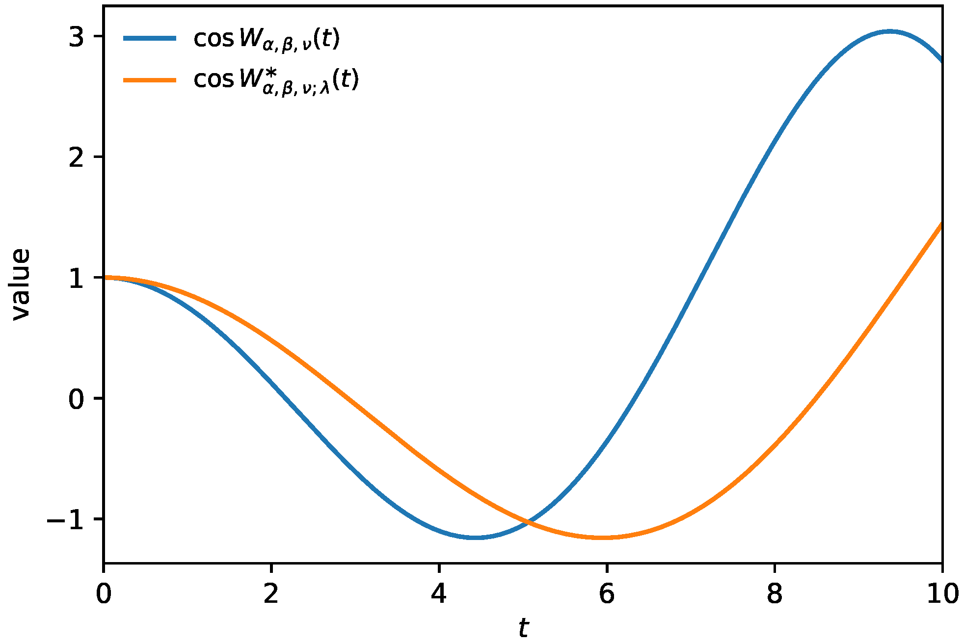
Table 2 reports representative pointwise values of the non-degenerate reference solution and its modified-degenerate counterpart for $\lambda =0.5$. These values complement Figure 1 by quantifying the effect of the scaling relation in Proposition 4 at selected time points. In particular, the last column shows that the modified-degenerate response does not differ from the reference curve by a uniform vertical shift; rather, the difference changes sign and magnitude as t increases, reflecting the $\lambda$-dependent time rescaling of the underlying non-degenerate W–oscillator profile.

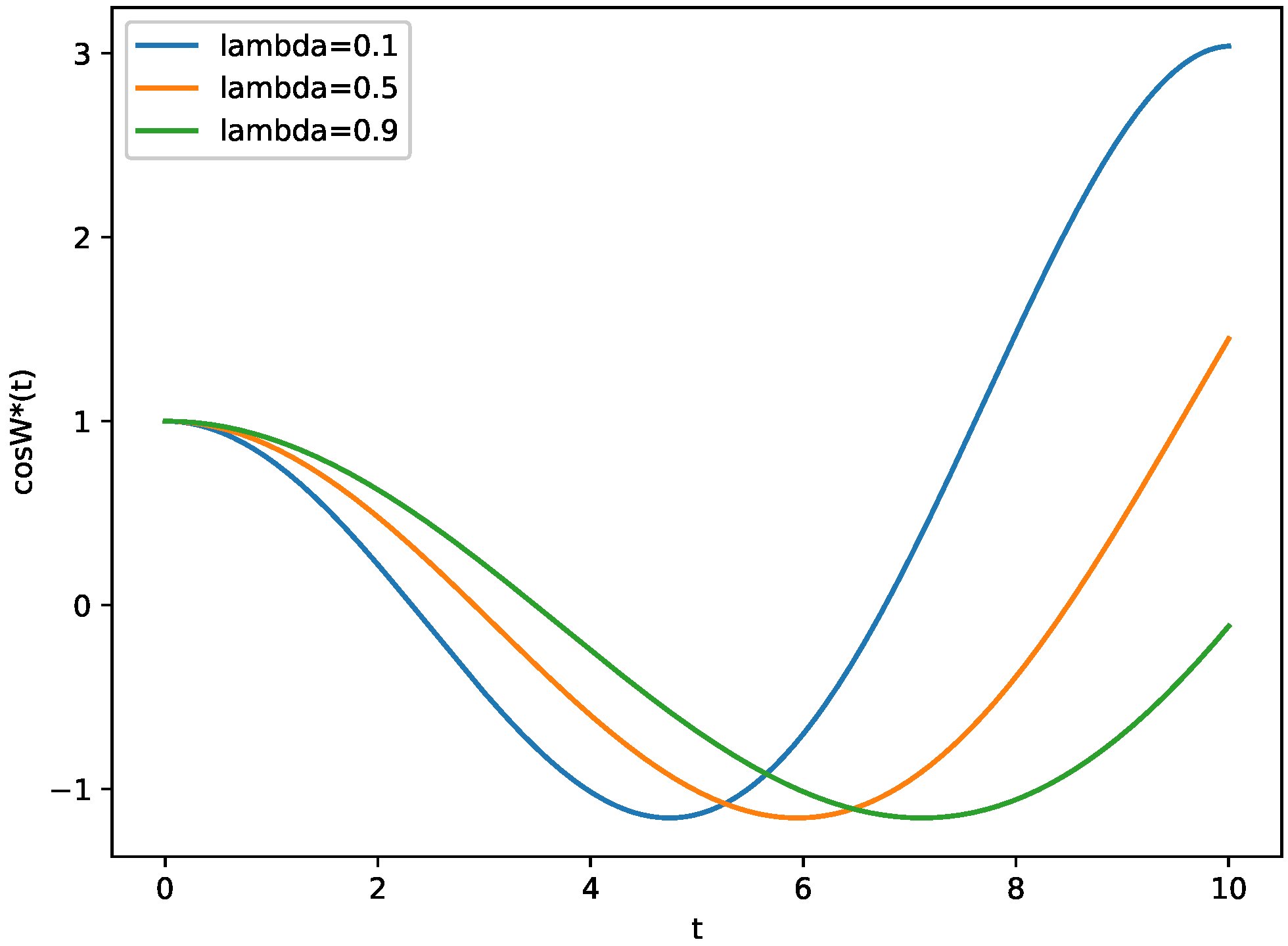
For the values shown in Figure 2, the corresponding time-stretch factors are $b_{0.2}^{\alpha +\beta }\approx 1.1383$, $b_{0.5}^{\alpha +\beta }\approx 1.3410$, and $b_{0.8}^{\alpha +\beta }\approx 1.5396$. Thus, increasing $\lambda$ does not change the shape of the underlying non-degenerate profile; it shifts the oscillation scale to the right in a quantitatively predictable way, exactly as stated by Proposition 4. This is the sense in which the numerical parameter study should be read.

7.2. A Volterra Equation with Polynomial Memory

Here, we use the convolution theorem for the modified-degenerate Laplace transform to solve a Volterra integral equation with polynomial memory, obtaining an explicit solution in terms of the induced W-type functions. This type of example is also physically meaningful: convolution equations are canonical hereditary models in which the kernel encodes memory, as in linear viscoelasticity, relaxation/dissipation, and diffusion-wave processes with after-effects [14,15,28]. Choosing polynomial memory keeps the analysis fully explicit while preserving the nonlocal-in-time structure that is central in applications.

One reason to use ${\mathcal{L}}_{\lambda }^{*}$ is its convolution theorem [20]. Let $(f\ast g)\left(t\right)={\int }_0^{t}f\left(\tau \right)g(t-\tau )d\tau$. For general background on resolvent kernels and Neumann-series solutions of Volterra equations, see [28].

Remark 7.

Lemma 1 shows that ${\mathcal{L}}_{\lambda }^{*}$ is the classical Laplace transform evaluated at ${\rho }_{\lambda }\left(s\right)$. Hence, the convolution theorem is the usual Laplace convolution theorem written in the variable s.

Consider the Volterra equation:

$$u\left(t\right)=h\left(t\right)+(\kappa \ast u)\left(t\right),$$

(56)

where h and $\kappa$ are given kernels. Assume that ${\mathcal{L}}_{\lambda }^{*}$ exists for $u,h,\kappa$ and that the convolution rule applies. Taking ${\mathcal{L}}_{\lambda }^{*}$ on both sides gives:

$$U\left(s\right)=H\left(s\right)+K\left(s\right)U\left(s\right)\Rightarrow U\left(s\right)={\displaystyle \frac{H\left(s\right)}{1-K\left(s\right)}}.$$

Fix $m\in {\mathbb{N}}_0$ and set:

$${\kappa }_m\left(t\right):={\displaystyle \frac{t^m}{m!}}(t\ge 0).$$

Using the monomial rule (12), we obtain:

$$K_m\left(s\right)={\mathcal{L}}_{\lambda }^{*}\left\{{\kappa }_m\right\}\left(s\right)=A_{\lambda }{\left(s\right)}^{m+1}.$$

(57)

For $\Re \left({\rho }_{\lambda }\left(s\right)\right)$ large, we have $|A_{\lambda }\left(s\right)|<1$, so that:

$${\displaystyle \frac{1}{1-K_m\left(s\right)}}={\displaystyle \sum _{j=0}^{\infty }}{A}_{\lambda }{\left(s\right)}^{j(m+1)}.$$

If, in addition, $h\left(t\right)={\mathrm{ExpW}}_{\alpha ,\beta ,\nu ;\lambda }^{*}\left(ct\right)$, then by (35):

$$H\left(s\right)=A_{\lambda }\left(s\right){\Psi }_{\alpha ,\beta ,\nu ;\lambda }^{*}\left(c{A}_{\lambda }\left(s\right)\right),$$

and therefore:

$$U\left(s\right)={\displaystyle \sum _{j=0}^{\infty }}{A}_{\lambda }{\left(s\right)}^{j(m+1)+1}{\Psi }_{\alpha ,\beta ,\nu ;\lambda }^{*}\left(c{A}_{\lambda }\left(s\right)\right).$$

(58)

Expanding ${\Psi }^{*}$ by (32) and inverting termwise with (12) yields the explicit series representation:

$$u\left(t\right)={\displaystyle \sum _{j=0}^{\infty }}{\displaystyle \sum _{n=0}^{\infty }}{c}^n{\displaystyle \frac{n!}{{\left[n\right]}_{\alpha ,\beta ,\nu ;\lambda }^{*}!}}{\displaystyle \frac{t^{n+j(m+1)}}{(n+j(m+1\left)\right)!}}.$$

(59)

Proposition 12.

For every fixed $t\ge 0$, the double series (59) converges absolutely. More precisely:

$${\displaystyle \sum _{j=0}^{\infty }}{\displaystyle \sum _{n=0}^{\infty }}\left|c^n{\displaystyle \frac{n!}{{\left[n\right]}_{\alpha ,\beta ,\nu ;\lambda }^{*}!}}{\displaystyle \frac{t^{n+j(m+1)}}{(n+j(m+1\left)\right)!}}\right|\le {\mathrm{ExpW}}_{\alpha ,\beta ,\nu ;\lambda }^{*}\left(\right|c\left|t\right){\displaystyle \sum _{j=0}^{\infty }}{\displaystyle \frac{t^{j(m+1)}}{\left(j\right(m+1\left)\right)!}}<\infty .$$

(60)

Hence, (59) defines a legitimate solution candidate term by term. If, in addition, $\alpha +\beta >1$ and $|A_{\lambda }\left(s\right)|<1$, then the Neumann expansion of $1/(1-K_m\left(s\right))$, the expansion of ${\Psi }^{*}$, and the corresponding termwise transform/inversion steps are all justified by absolute convergence.

Proof. 

Let $k=j(m+1)$. Since $(n+k)!\ge n!k!$, we have:

$$\left|c^n{\displaystyle \frac{n!}{{\left[n\right]}^{*}!}}{\displaystyle \frac{t^{n+k}}{(n+k)!}}\right|\le {\displaystyle \frac{{\left(\right|c\left|t\right)}^n}{{\left[n\right]}^{*}!}}{\displaystyle \frac{t^k}{k!}}.$$

Summing first over n and then over j gives exactly (60). The first factor is ${\mathrm{ExpW}}_{\alpha ,\beta ,\nu ;\lambda }^{*}\left(\right|c\left|t\right)$, which is finite by Theorem 1, and the second factor is a subseries of $e^t$. This proves absolute convergence of (59). If $\alpha +\beta >1$, then Proposition 9 shows that ${\Psi }^{*}$ is whole; so, together with $|A_{\lambda }\left(s\right)|<1$, the geometric factor and the factorial-ratio series are absolutely convergent in the transform domain. The stated interchanges then follow from the same Tonelli/dominated-convergence arguments used earlier in Section 6. □

Remark 8.

The Neumann-series point of view corresponds to $u={\sum }_{j=0}^{\infty }{\kappa }_m^{\ast j}\ast h$. In the present polynomial case, one has the closed form ${\kappa }_m^{\ast j}\left(t\right)=t^{j(m+1)-1}/(j(m+1)-1)!$ for $j\ge 1$, which follows immediately from (57) and the monomial rule (12).

7.2.1. Complete Worked Example: The Case $m=1$

We now spell out the inversion in a concrete case. Let:

$${\kappa }_1\left(t\right)=t,\mathrm{so}\mathrm{that}{K}_1\left(s\right)=A_{\lambda }{\left(s\right)}^2={\displaystyle \frac{1}{{\rho }_{\lambda }{\left(s\right)}^2}}.$$

Then:

$$U\left(s\right)={\displaystyle \frac{H\left(s\right)}{1-A_{\lambda }{\left(s\right)}^2}}=H\left(s\right)\left(1+{\displaystyle \frac{1}{{\rho }_{\lambda }{\left(s\right)}^2-1}}\right).$$

(61)

Since the classical Laplace transform satisfies:

$$\mathcal{L}\left\{\sinh t\right\}\left(p\right)={\displaystyle \frac{1}{p^2-1}}(\Re \left(p\right)>1),$$

Lemma 1 yields:

$${\mathcal{L}}_{\lambda }^{*}\left\{\sinh t\right\}\left(s\right)={\displaystyle \frac{1}{{\rho }_{\lambda }{\left(s\right)}^2-1}}.$$

(62)

Combining (61) and (62), we obtain the explicit resolvent formula:

$$u\left(t\right)=h\left(t\right)+(\sinh \ast h)\left(t\right)=h\left(t\right)+{\int }_0^t\sinh (t-\tau )h\left(\tau \right)d\tau .$$

(63)

If we now choose $h\left(t\right)={\mathrm{ExpW}}_{\alpha ,\beta ,\nu ;\lambda }^{*}\left(ct\right)$, then:

$$h\left(\tau \right)={\displaystyle \sum _{n=0}^{\infty }}{\displaystyle \frac{c^n{\tau }^n}{{\left[n\right]}_{\alpha ,\beta ,\nu ;\lambda }^{*}!}},\sinh (t-\tau )={\displaystyle \sum _{j=0}^{\infty }}{\displaystyle \frac{{(t-\tau )}^{2j+1}}{(2j+1)!}}.$$

Substituting these series into (63) and integrating term by term gives:

$$u\left(t\right)={\mathrm{ExpW}}_{\alpha ,\beta ,\nu ;\lambda }^{*}\left(ct\right)+{\displaystyle \sum _{j=0}^{\infty }}{\displaystyle \sum _{n=0}^{\infty }}{\displaystyle \frac{c^n}{{\left[n\right]}_{\alpha ,\beta ,\nu ;\lambda }^{*}!}}{\displaystyle \frac{1}{(2j+1)!}}{\int }_0^t{(t-\tau )}^{2j+1}{\tau }^{n}d\tau .$$

Using the beta-integral identity:

$${\int }_0^t{(t-\tau )}^{2j+1}{\tau }^{n}d\tau =t^{n+2j+2}{\displaystyle \frac{(2j+1)!n!}{(n+2j+2)!}},$$

we arrive at:

$$u\left(t\right)={\mathrm{ExpW}}_{\alpha ,\beta ,\nu ;\lambda }^{*}\left(ct\right)+{\displaystyle \sum _{j=0}^{\infty }}{\displaystyle \sum _{n=0}^{\infty }}{c}^n{\displaystyle \frac{n!}{{\left[n\right]}_{\alpha ,\beta ,\nu ;\lambda }^{*}!}}{\displaystyle \frac{t^{n+2j+2}}{(n+2j+2)!}}.$$

Re-indexing with $k=j+1$ shows that this is exactly the $m=1$ specialization of (59):

$$u\left(t\right)={\displaystyle \sum _{k=0}^{\infty }}{\displaystyle \sum _{n=0}^{\infty }}{c}^n{\displaystyle \frac{n!}{{\left[n\right]}_{\alpha ,\beta ,\nu ;\lambda }^{*}!}}{\displaystyle \frac{t^{n+2k}}{(n+2k)!}}.$$

(64)

Thus, the inversion is completely explicit in this case: the resolvent kernel is $\sinh t$, and the analytic series solution follows by direct termwise convolution.

7.2.2. Numerical Example and Residual Check

We next evaluate the explicit series (64) and verify numerically that it satisfies (56). Choose:

$$(\alpha ,\beta ,\nu )=(0.6,0.8,1.2),\lambda =0.5,m=1,c=0.7,$$

so that ${\kappa }_1\left(t\right)=t$ and $h\left(t\right)={\mathrm{ExpW}}_{\alpha ,\beta ,\nu ;\lambda }^{*}\left(ct\right)$. We approximate (64) by truncating the double sum to $0\le n\le 50$ and $0\le j\le 40$ and evaluate $({\kappa }_1\ast u)\left(t\right)$ by a composite trapezoidal rule on $[0,t]$ with step size $\Delta t=5\times {10}^{-3}$. A representative truncation study at $t=5$ is reported in Table 3; the values stabilize very rapidly, with the change dropping from $2.4\times {10}^{-6}$ to below ${10}^{-40}$ over the displayed truncations. 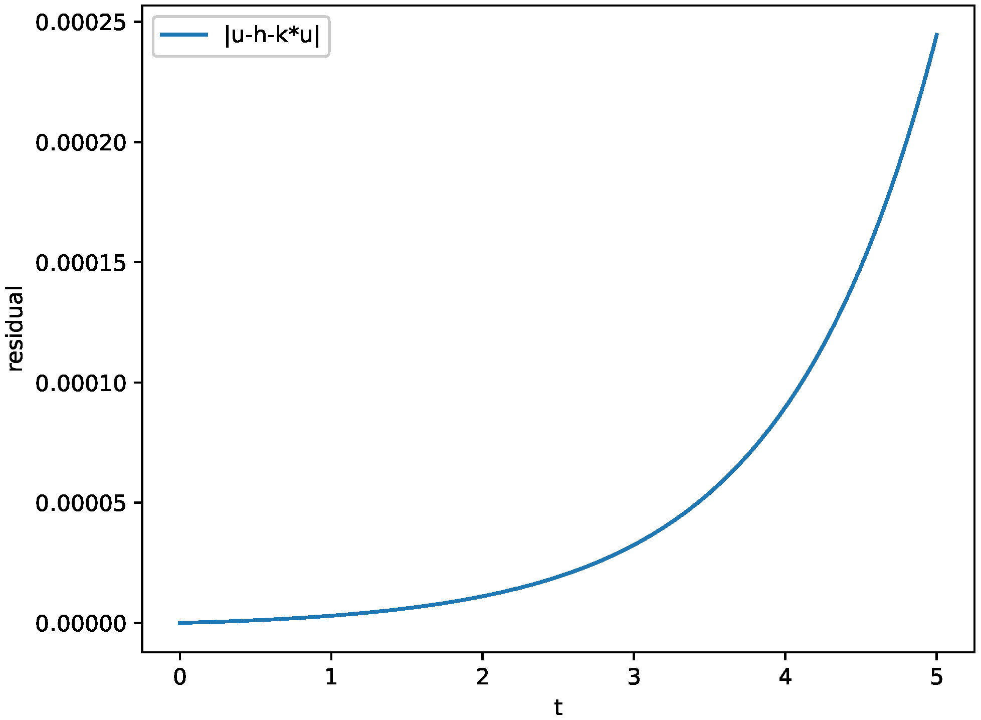On $t\in [0,5]$, the maximum absolute residual:

$$R\left(t\right):=u\left(t\right)-h\left(t\right)-({\kappa }_1\ast u)\left(t\right)$$

is ${max}_{[0,5]}\left|R\left(t\right)\right|\approx 2.5\times {10}^{-4}$.

This residual should be interpreted as a numerical consistency check rather than as an independent proof of the analytic solution: it measures the mismatch between two separate approximations, namely the truncated series for u and the numerical quadrature for the convolution term. The mild growth of $\left|R\right(t\left)\right|$ near the right end of the interval is caused by the rapid growth of $u\left(t\right)$ itself; for example, Table 4 gives $u\left(5\right)\approx 1.17\times {10}^2$; so, the endpoint residual is only about $2.1\times {10}^{-6}$ in relative size.

To add an independent benchmark, we also solved (56) by a direct marching quadrature method on a uniform grid with step size $\Delta t={10}^{-3}$. Since the kernel is ${\kappa }_1\left(t\right)=t$, the discretized Volterra integral contains no implicit $u\left(t_i\right)$ term at the right endpoint; so, the nodal values can be computed sequentially from left to right. Denoting this second approximation by $u_{\mathrm{num}}$, we found that the absolute difference between the analytic truncated series and the direct solver stays below $2.8\times {10}^{-5}$ on the sampled grid $t=0,0.05,0.10,\dots ,5.00$. 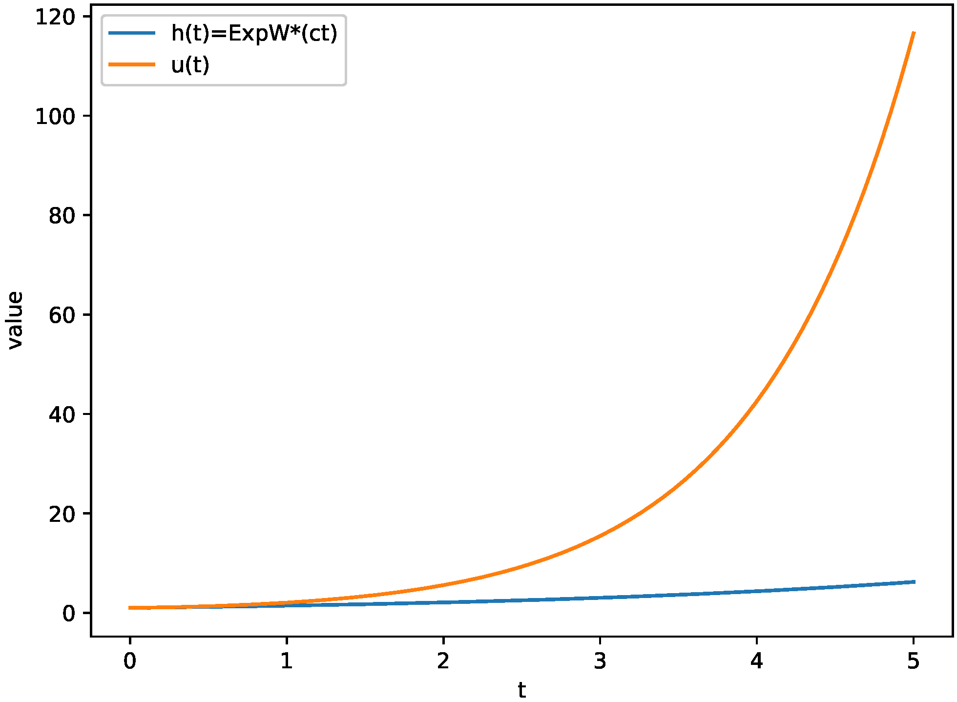Representative values are listed in Table 5. This comparison is not used to derive the closed form; it is included only as an external numerical check that the explicit series solution is consistent with a standard solver for Volterra equations. The forcing and solution profiles used in this check are shown in Figure 3, and the corresponding residual curve is shown in Figure 4.

8. Discussion

The main message of this manuscript is best understood as a transport principle. Replacing $\Gamma$ by ${\Gamma }_{\lambda }^{*}$ does not generate a new independent W-function hierarchy; rather, it moves the existing $W_{\alpha ,\beta ,\nu }$ framework into the modified-degenerate spectral setting by an exact scaling. This point is important in relation to the recent literature. Relative to [4], the present work does not extend the analytic class of Wright-type objects. Relative to studies on degenerate and modified-degenerate Laplace integrals, however, it supplies a self-contained operational calculus written directly in the native variable s of ${\mathcal{L}}_{\lambda }^{*}$.

From a methodological perspective, the value of this paper therefore lies in explicit formulas and transparent bookkeeping. Once the scaling relation is made precise, the transform pairs, convolution rule, and coefficient-shift operator can all be transported from the classical setting without ambiguity. This also explains the role of the two worked examples: they are intended as benchmark operational problems showing how the formalism behaves in oscillator and Volterra-memory settings that resemble standard hereditary models from applied analysis.

The same mechanism also marks the limitations of the present study. Because the deformation is an exact rescaling, the modified-degenerate families do not exhibit fundamentally new growth, zero, or singularity patterns beyond those of the non-degenerate theory. Likewise, the W-derivative introduced here should be read as a formal series operator rather than as a closed-form differential operator in the classical sense. These limitations are not weaknesses of the derivation; they define precisely the scope of the contribution.

In view of this, genuinely new analytic phenomena are more likely to arise in the degenerate gamma/Laplace framework of [21], where the simple rescaling mechanism is absent. This is also the most natural route if one wishes to go beyond the transport principle established here: once the multiplicative scaling identity fails, the factorial, the induced W-functions, and their transform theory can no longer be reduced to the non-degenerate case by a single change in variables. Other natural directions include the study of growth and zero distributions via Proposition 4, numerical inversion in more general memory-kernel problems, and extensions to broader fractional and variable-coefficient models with nonclassical convolution structures.

9. Conclusions

We introduced a modified-degenerate analogue of the $W_{\alpha ,\beta ,\nu }$-factorial and the associated exponential, trigonometric, and hyperbolic families. The central structural result is that ${\Gamma }_{\lambda }^{*}\left(s\right)=b_{\lambda }^s\Gamma \left(s\right)$; so, the entire construction is an exact rescaling of the non-degenerate $W_{\alpha ,\beta ,\nu }$ theory rather than a genuinely new transcendental family. In concrete terms, Propositions 3 and 4 show that both the factorial and the induced functions are transported from the known theory by a single scaling parameter.

Within that rescaled framework, we derived explicit modified-degenerate Laplace-transform identities, proved the inherited convolution theorem, quantified the limit $\lambda \to 0^{+}$, clarified the formal W-shift operator, and developed operational examples including a complete Volterra case with numerical consistency checks. In this sense, this paper contributes a precise operational reformulation of the existing W-theory in the ${\mathcal{L}}_{\lambda }^{*}$ setting.

References

- Haubold, H.J.; Mathai, A.M.; Saxena, R.K. Mittag-Leffler functions and their applications. J. Appl. Math. 2011, 2011, 298628. [Google Scholar] [CrossRef] [Scilit]
- Kilbas, A.A. Fractional calculus of the generalized Wright function. Fract. Calc. Appl. Anal. 2005, 8, 113–126. [Google Scholar]
- Kiryakova, V. A guide to special functions in fractional calculus. Mathematics 2021, 9, 106. [Google Scholar] [CrossRef] [Scilit]
- Droghei, R.; Garra, R. Wα,β,ν trigonometric and hyperbolic generalized functions. Integral Transform. Spec. Funct. 2025, 37, 225–248. [Google Scholar] [CrossRef] [Scilit]
- Wright, E.M. The asymptotic expansion of the generalized hypergeometric function. J. Lond. Math. Soc. 1935, 10, 286–293. [Google Scholar] [CrossRef] [Scilit]
- Wright, E.M. The generalized Bessel function of order greater than one. Q. J. Math. 1940, 11, 36–48. [Google Scholar] [CrossRef] [Scilit]
- Aceto, L.; Durastante, F. Efficient computation of the Wright function and its applications to fractional diffusion-wave equations. ESAIM Math. Model. Numer. Anal. 2022, 56, 2181–2196. [Google Scholar] [CrossRef] [Scilit]
- Droghei, R. Properties of the multi-index special function . Fract. Calc. Appl. Anal. 2023, 26, 2057–2068. [Google Scholar] [CrossRef] [Scilit]
- Kiryakova, V.; Paneva-Konovska, J. Going next after “A guide to special functions in fractional calculus”: A discussion survey. Mathematics 2024, 12, 319. [Google Scholar] [CrossRef] [Scilit]
- Mainardi, F.; Consiglio, A. The Wright functions of the second kind in mathematical physics. Mathematics 2020, 8, 884. [Google Scholar] [CrossRef] [Scilit]
- Mainardi, F.; Paris, R.B.; Consiglio, A. Wright functions of the second kind and Whittaker functions. Fract. Calc. Appl. Anal. 2022, 25, 858–875. [Google Scholar] [CrossRef] [Scilit]
- Paneva-Konovska, J.; Kiryakova, V. The generalized Fox–Wright function: The Laplace transform, the Erdélyi–Kober fractional integral and its role in fractional calculus. Mathematics 2024, 12, 1918. [Google Scholar] [CrossRef] [Scilit]
- Bagley, R.L.; Torvik, P.J. Fractional calculus—A different approach to the analysis of viscoelastically damped structures. AIAA J. 1983, 21, 741–748. [Google Scholar] [CrossRef] [Scilit] [PubMed]
- Caputo, M.; Mainardi, F. A new dissipation model based on memory mechanism. Pure Appl. Geophys. 1971, 91, 134–147. [Google Scholar] [CrossRef] [Scilit]
- Mainardi, F. Fractional Calculus and Waves in Linear Viscoelasticity: An Introduction to Mathematical Models; Imperial College Press: London, UK, 2010. [Google Scholar]
- Podlubny, I. Fractional Differential Equations: An Introduction to Fractional Derivatives, Fractional Differential Equations, to Methods of Their Solution and Some of Their Applications; Mathematics in Science and Engineering; Academic Press: San Diego, CA, USA, 1999; Volume 198. [Google Scholar]
- Yağcı, O. Degenerate Mittag–Leffler functions defined via the degenerate gamma function and applications to fractional Maxwell–Zener viscoelasticity. Anal. Math. Phys. 2026, 16, 46. [Google Scholar] [CrossRef] [Scilit]
- Almalki, Y.; Abdalla, M.; Abd-Elmageed, H. Results on the modified degenerate Laplace-type integral associated with applications involving fractional kinetic equations. Demonstr. Math. 2023, 56, 20230112. [Google Scholar] [CrossRef] [Scilit]
- Campos, H.J.; Fernandez, J.C.; Natuil, J.B.M. On degenerate Laplace-type integral transform. Eur. J. Pure Appl. Math. 2023, 16, 2213–2233. [Google Scholar] [CrossRef] [Scilit]
- Kim, Y.; Kim, B.M.; Jang, L.-C.; Kwon, J. A note on modified degenerate gamma and Laplace transformation. Symmetry 2018, 10, 471. [Google Scholar] [CrossRef] [Scilit]
- Kim, T.; Kim, D.S. Degenerate Laplace transform and degenerate gamma function. Russ. J. Math. Phys. 2017, 24, 241–248. [Google Scholar] [CrossRef] [Scilit]
- Yağcı, O.; Khan, W.A.; Mohamed, K.S.; Iqbal, A.; Koh, W.S. Degenerate two-variable q-Legendre polynomials via q-operational calculus and degenerate Laplace/Sumudu transforms. AIMS Math. 2026, 11, 7207–7234. [Google Scholar] [CrossRef] [Scilit]
- Yağcı, O.; Şahin, R. Degenerate Pochhammer symbol, degenerate Sumudu transform, and degenerate hypergeometric function with applications. Hacet. J. Math. Stat. 2021, 50, 1448–1465. [Google Scholar] [CrossRef] [Scilit]
- Ege, İ. Modified Laplace-type transform and its properties. Eur. J. Pure Appl. Math. 2025, 18, 5986. [Google Scholar] [CrossRef] [Scilit]
- Jarad, F.; Abdeljawad, T. A modified Laplace transform for certain generalized fractional operators. Results Nonlinear Anal. 2018, 1, 88–98. [Google Scholar]
- Olver, F.W.J.; Daalhuis, A.B.O.; Lozier, D.W.; Schneider, B.I.; Boisvert, R.F.; Clark, C.W.; Miller, B.R.; Saunders, B.V.; Cohl, H.S.; McClain, M.A. (Eds.) NIST Digital Library of Mathematical Functions; Version 1.2.5 (release date 2025-12-15); National Institute of Standards and Technology: Gaithersburg, MD, USA, 2025. Available online: https://dlmf.nist.gov/ (accessed on 5 January 2026).
- Widder, D.V. The Laplace Transform, 2nd ed.; Princeton Mathematical Series; Princeton University Press: Princeton, NJ, USA, 1946; Volume 6. [Google Scholar]
- Gripenberg, G.; Londen, S.-O.; Staffans, O. Volterra Integral and Functional Equations; Encyclopedia of Mathematics and its Applications; Cambridge University Press: Cambridge, UK, 1990; Volume 34. [Google Scholar]