Adaptive Label Reweighting via Boundary-Aware Meta Learning for Long-Tail Legal Element Recognition

Abstract

Legal element recognition, which identifies discrete factual elements in Chinese court judgments to support judicial analysis and case retrieval, faces a severe long-tail challenge: head-to-tail label-frequency ratios exceed 100:1, and over 60% of sentences carry no label, starving rare elements of training signal. Static reweighting methods assign fixed weights prior to training and cannot respond to the model’s evolving confidence; sample-level meta-learning couples all co-occurring label gradients to a single scalar, preventing independent tail-label amplification. We propose BML-Trans, a boundary-aware meta-learning framework that addresses both limitations. A label-wise meta-weighting mechanism maintains per-label gradient weights updated via bilevel hypergradient descent, decoupling tail-label amplification from co-occurring head labels. A boundary-aware meta-set concentrates calibration signal on high-uncertainty, tail-triggering sentences rather than on easy negatives, and a lightweight Multi-Scale Adapter sharpens the warm-up probability estimates on which boundary selection depends. Concretely, BML-Trans achieves an average Avg-F1 of 82.5% on CAIL2019 across the labor, divorce, and loan domains, outperforming the strongest baseline by 1.2 percentage points overall and by up to 5.7 percentage points on tail-label Macro-F1, at only 14% additional training cost. Ablation confirms a cascade dependency among the three components, establishing that the gains are structural rather than incidental to threshold selection or initialization.

1. Introduction

Scaling legal reasoning to the millions of judgment documents produced annually by Chinese courts requires structured representations of the case facts currently locked in unstructured natural language [1,2]. Downstream applications such as similar-case retrieval, charge prediction, and sentencing assistance operate on discrete factual elements (e.g., employment duration, disputed amount, custody arrangement), yet the fact-description sections of judgment documents record these elements in free-form prose without explicit annotation. Legal element recognition, the task of tagging each sentence with the factual elements it conveys, is therefore the extraction bottleneck that determines how much of the judicial record becomes accessible to computational legal analysis. It is naturally formalized at the sentence level multi-label classification, where each civil-law domain imposes its own label schema over the factual elements specific to that area of law [3]. Stated as a machine learning problem, each sentence is an instance that may be assigned zero or more labels from a fixed schema of K domain-specific elements, making legal element recognition a canonical instance of multi-label text classification [4].

Two structural properties of legal judgment corpora make this task substantially harder than balanced multi-label benchmarks. In a long-tail distribution, a small set of head classes dominate training data while the majority of tail classes each appear very infrequently [5]; this imbalance is well studied in visual recognition but is equally acute in specialized legal NLP corpora. The label distribution is severely long-tailed: head-to-tail frequency ratios consistently exceed $100:1$, with the rarest labels having as few as 50 positive training instances [3]. Simultaneously, more than 60% of sentences carry no label at all [3], so that under binary cross-entropy (BCE) training every label dimension receives overwhelmingly negative gradients at each update. These two forces reinforce each other: the negative-gradient mass drives predictions toward all-zero outputs, while the already-sparse positive gradients of tail labels are further diluted, leaving the model with almost no informative signal near the decision boundaries of rare elements. The resulting symptom is a wide gap between Micro F1 and Macro F1 in which the rarest elements account for the largest per-label errors.

Loss reweighting is the most direct response to this imbalance. Class-Balanced Loss [6] scales each label by its inverse effective sample count; Asymmetric Loss [7] further suppresses easy-negative contributions through a shifted focusing term. These methods improve Macro F1 in moderately imbalanced regimes, but their weights are computed once from corpus-level frequencies and remain fixed throughout training, unable to shift toward the decision-boundary samples that become increasingly informative as the model improves. Other non-adaptive strategies share a related limitation: oversampling [8] increases tail-label exposure but amplifies head-label gradients in multi-label sentences alongside them; contrastive representation learning [9] improves embedding separability but does not redistribute the gradient magnitude across co-occurring labels during loss computation; post-hoc confidence calibration [10] adjusts prediction scores after training but cannot recover the representational quality lost to the gradient imbalance accumulated during optimization. What all these approaches lack is a mechanism that adapts during training and operates at label-wise granularity within multi-label instances.

Meta-learning reweighting provides the missing adaptivity by deriving instance weights from a held-out meta-set at each training step. Ren et al. [11] assign a scalar weight to each training sample and update it by differentiating through one gradient step on the meta-set loss; Meta-Weight-Net [12] extends this idea by parameterizing the mapping as a learned network. Both approaches have advanced single-label long-tail recognition, yet a per-sample scalar weight amplifies all label gradients in that sample uniformly: when a head label and a tail label co-occur in one sentence, the tail label’s gradient cannot be independently adjusted. A second limitation concerns the meta-set itself: random or class-balanced sampling inherits the training distribution’s imbalance, producing a gradient signal dominated by easy negatives and head labels rather than by the tail-label boundary instances where the calibration signal is most needed. Effective meta-reweighting in this setting, therefore, requires two properties that no existing method provides jointly: label-wise weight granularity for intra-sentence gradient decoupling, and a meta-set concentrated on the tail-label decision boundaries for stable hypergradient direction.

We propose Boundary-aware Meta-Learning Transformer (BML-Trans) to satisfy both requirements within a single training framework. The “meta-learning” in BML-Trans refers specifically to label-wise meta-weighting (the title component “Label-Wise Meta-Weighting”), implemented via a bilevel update on a per-label weight vector calibrated against boundary-selected sentences. BML-Trans replaces per-sample weights with per-label weights updated via bilevel hypergradient descent against a curated meta-set, enabling the optimizer to amplify a tail label’s gradient independently of co-occurring head labels. The meta-set is constructed by selecting instances whose predictions lie near the decision boundary subject to a tail-label coverage constraint, ensuring that the gradient signal from the meta-set reflects tail-class difficulty rather than easy-negative dominance. The Multi-Scale Adapter, trained jointly during warm-up, improves early-stage probability estimates by enriching encoder representations at multiple convolutional scales, raising the quality of boundary-based selection in subsequent epochs and stabilising meta-weight updates.

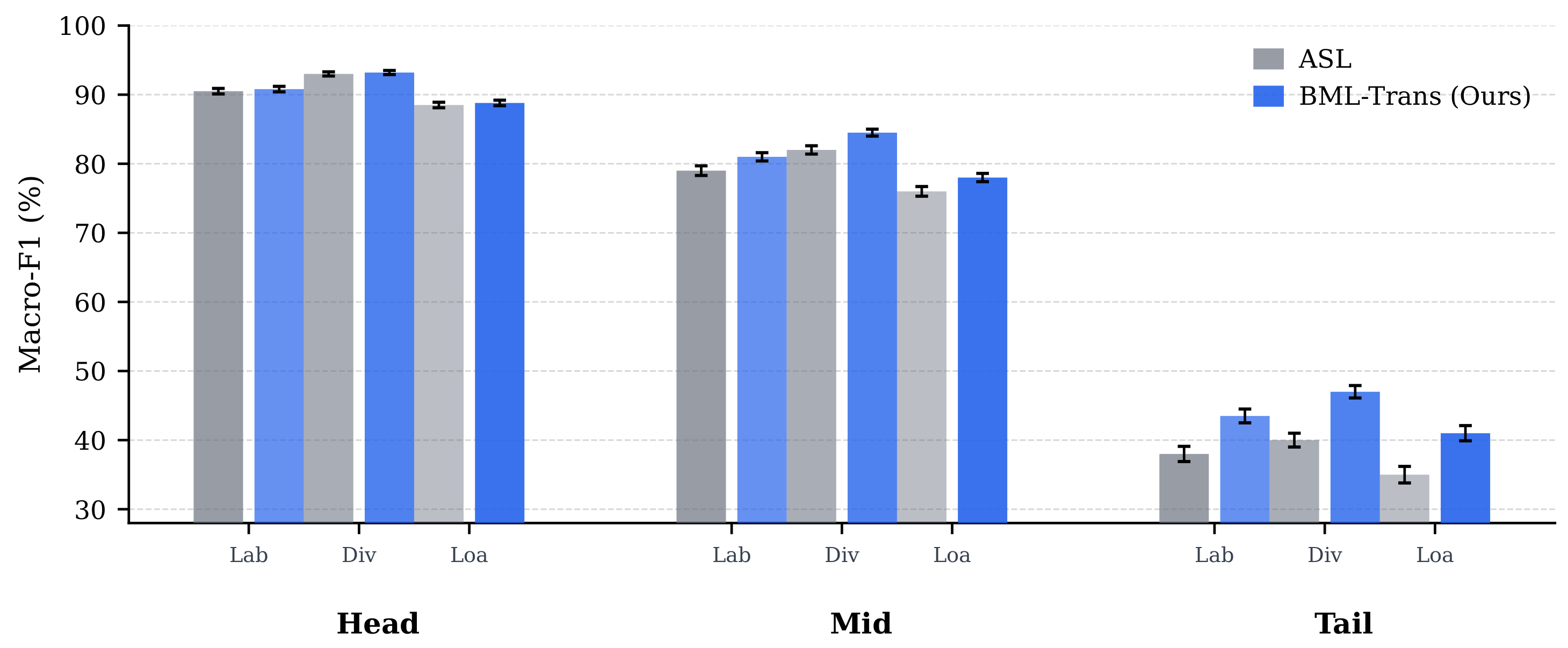
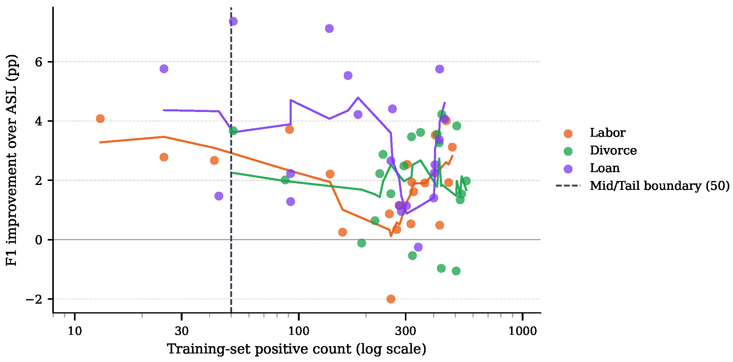
On all three CAIL2019 domains, BML-Trans improves tail-label Macro F1 by up to 5.7 percentage points over ASL, the strongest static-reweighting baseline, and by up to 3.6 percentage points over Ren et al., the strongest sample-level meta-learning baseline, while maintaining competitive Micro F1 at only 14% additional training cost. Ablation experiments reveal a cascade dependency among the three components: removing the boundary meta-set calibration degrades meta-set quality, which in turn reduces the effectiveness of label-wise meta-weighting. Our main contributions are as follows:

• A label-wise meta-weighting mechanism, updated via a one-step bilevel gradient descent, that independently scales each label’s gradient contribution within a shared training sentence, dissolving the per-sample coupling that prevents existing meta-reweighting methods from amplifying tail-label gradients without simultaneously inflating those of co-occurring head labels.
• A boundary-aware meta-set construction procedure that selects calibration sentences by jointly scoring model uncertainty, prediction loss, and tail-trigger density, subject to a per-tail-label coverage constraint; the Multi-Scale Adapter trained during warm-up sharpens early probability estimates, which in turn raises meta-set quality and stabilizes hypergradient direction, a cascade dependency that the ablation study quantifies across all three domains.
• Disaggregated evaluation across Head, Mid, and Tail frequency buckets on all three CAIL2019 domains, showing that BML-Trans improves Tail Macro-F1 by up to 5.7 percentage points over the strongest static-reweighting baseline and by up to 3.6 percentage points over sample-level meta-reweighting, at only 14% additional training cost, with mechanistic analyses confirming that the gains originate from the bilevel optimization rather than threshold selection or favorable seeds.

The rest of this paper is organized as follows. Section 2 reviews legal element recognition, imbalance handling in multi-label classification, meta-learning reweighting, and multi-scale representations. Section 3 formulates the task, describes the Multi-Scale Adapter and label-wise meta-weighting, and presents the boundary meta-set construction procedure. Section 4 reports setup, main results, long-tail and ablation analyses, and mechanistic findings. Section 6 summarizes the contributions and limitations.

2. Related Work

2.1. Legal Element Recognition and Legal Text Classification

Legal element recognition has been studied as part of the broader research agenda on legal intelligence in China, catalyzed by the CAIL series of shared tasks [3]. Early work relied on feature engineering with support vector machines or conditional random fields; subsequent work adopted CNN [13] and BiLSTM architectures; and the emergence of pre-trained language models, particularly BERT [14], RoBERTa [15], and MacBERT [16], substantially raised baseline performance. Liu et al. [17] demonstrated that fine-tuning MacBERT-base on the CAIL2019 formulation achieves strong Micro-F1 with a standard linear head, and Liu et al. [18] further incorporated a label correlation matrix into an XLNet-based [19] model to capture inter-label dependencies. Domain-specialized models such as Lawformer [20], Legal-RoBERTa [21], and LEGAL-BERT [22] provide additional pre-training signal for legal vocabulary and discourse, motivated by downstream tasks such as legal judgment prediction [1] and similar-case retrieval [2]. A common thread in all these works is the focus on aggregate metrics such as Micro-F1 or Avg-F1; none systematically addresses the long-tail distribution among the 20 domain-specific element labels or provides a controlled comparison of the head/mid/tail performance gap. Chalkidis et al. [23] show that severe label imbalance persists across jurisdictions and languages in MultiEURLEX, a 23-language multi-label legal benchmark, confirming that the challenge is not specific to Chinese legal corpora. This work addresses this limitation by introducing Tail Macro-F1 and head/mid/tail bucket metrics as primary evaluation criteria and by providing, to our knowledge, the first systematic comparison of imbalance-handling methods under these criteria on all three CAIL2019 domains.

2.2. Imbalance Handling in Multi-Label Text Classification

Static reweighting methods assign per-class weights before training based on frequency statistics. Focal Loss [24] introduced the idea of down-weighting well-classified examples with an adaptive focusing exponent, establishing the conceptual foundation for this family of methods. The pos_weight BCE sets each label’s positive weight to the ratio of negative to positive instances; Class-Balanced Loss [6] replaces raw frequency with the effective number of samples, which accounts for data overlap and produces smoother weights; and Asymmetric Loss [7] applies asymmetric focusing exponents to positive and negative predictions, optionally discarding very-easy negatives through a hard margin shift. ASL achieves strong results on large-scale multi-label benchmarks and serves as the most competitive static baseline in this work. A broader taxonomy of long-tail recognition strategies [5] encompasses Label-Distribution-Aware Margin Loss [25], which imposes larger decision margins for rare classes; decoupled representation and classification training [26]; logit adjustment at inference time [27]; Distribution-Balanced Loss [28]; and Bilateral-Branch Networks [29]. All static methods share the limitation that their weights are fixed before training and cannot respond to the model’s evolving confidence during optimization. A parallel line of work models label co-occurrence structure explicitly. Multi-label classification has a broad literature [4]; label-specific attention mechanisms have proven effective across domains such as clinical coding [30] and extreme text classification [31]. LSAN [32] constructs label-specific document representations through an attention mechanism guided by label embeddings, and supervised contrastive learning approaches [33,34] separate semantically similar but label-distinct sentences in the embedding space. While these structural methods improve label-discriminative representations, they do not address the fundamental heterogeneity in gradient magnitude allocation across labels with very different frequencies, a limitation that persists regardless of how well the encoder separates label embeddings. BML-Trans directly targets this gap through label-wise gradient reweighting; the two approaches are complementary, and combining correlation-aware architectures with boundary meta-set calibration remains an open direction. On the generative side, LTGC [35] uses LLMs to synthesize diverse tail-class content and fine-tunes the classifier on the augmented data, achieving strong gains on long-tail benchmarks; the same principle extends naturally to text classification settings.

2.3. Meta-Learning and Bilevel Optimization for Reweighting

Bilevel programming provides the theoretical foundation for meta-learning-based hyperparameter optimization [36], and model-agnostic meta-learning [37] demonstrated that gradient-based inner-outer loop updates generalize across diverse adaptation tasks. Ren et al. [11] show that the bilevel program of finding sample weights that minimize the meta-loss after one gradient step on the weighted training loss can be solved approximately via one-step gradient unrolling. Meta-Weight-Net [12] replaces per-example scalars with a small network that maps loss values to weights, enabling generalization across the loss range. Both methods were developed primarily for noisy-label learning and single-label classification; neither has been systematically studied in multi-label long-tail settings. Both frameworks operate at sample granularity and construct the meta-set by random partition, two design choices that are suboptimal for the multi-label long-tail setting, as argued in Section 1. BML-Trans addresses both gaps simultaneously: it shifts weight assignment from sample to label granularity, and it constructs the meta-set to concentrate calibration signal on high-uncertainty, tail-triggering sentences rather than sampling uniformly. Guo et al. [38] avoid bilevel gradient steps entirely by casting reweighting as an optimal transport problem, decoupling weight learning from the classifier and achieving competitive results across image, text, and point cloud benchmarks.

2.4. Multi-Scale Adapter Representations

Legal sentences simultaneously contain short local triggers (specific legal terms and named numerical conditions) and long-range contextual dependencies. Inception-style architectures in computer vision [39] pioneered the idea of processing feature maps at multiple spatial resolutions in parallel, and analogous constructions have been explored in NLP. Depth-wise separable convolutions [40] reduce parameter counts relative to standard convolutions while preserving receptive-field coverage, making them suitable for lightweight adapter modules on top of large Transformer [41] encoders. Adapter-based methods [42] insert lightweight modules between PLM layers to capture task-specific patterns with minimal parameter overhead. The Multi-Scale Adapter in BML-Trans belongs to this family: it places depth-wise separable convolutions at kernel sizes 3, 5, and 7 after the final encoder layer and gates the residual addition with a sigmoid scalar, introducing fewer than 2% additional parameters relative to MacBERT-base. Prior adapter-based NLP methods typically apply a single bottleneck transformation at a fixed receptive field; by processing the sequence at three convolutional scales in parallel, the Multi-Scale Adapter fills the gap between global attention and local pattern capture at varying span lengths, a distinction that matters for legal element triggers, which range from single-token numerical conditions to multi-token named-entity phrases. This deliberate minimality also ensures that the adapter’s contribution can be cleanly isolated in ablation studies, separating its effect from the bilevel optimization mechanism.

3. Method

3.1. Overview

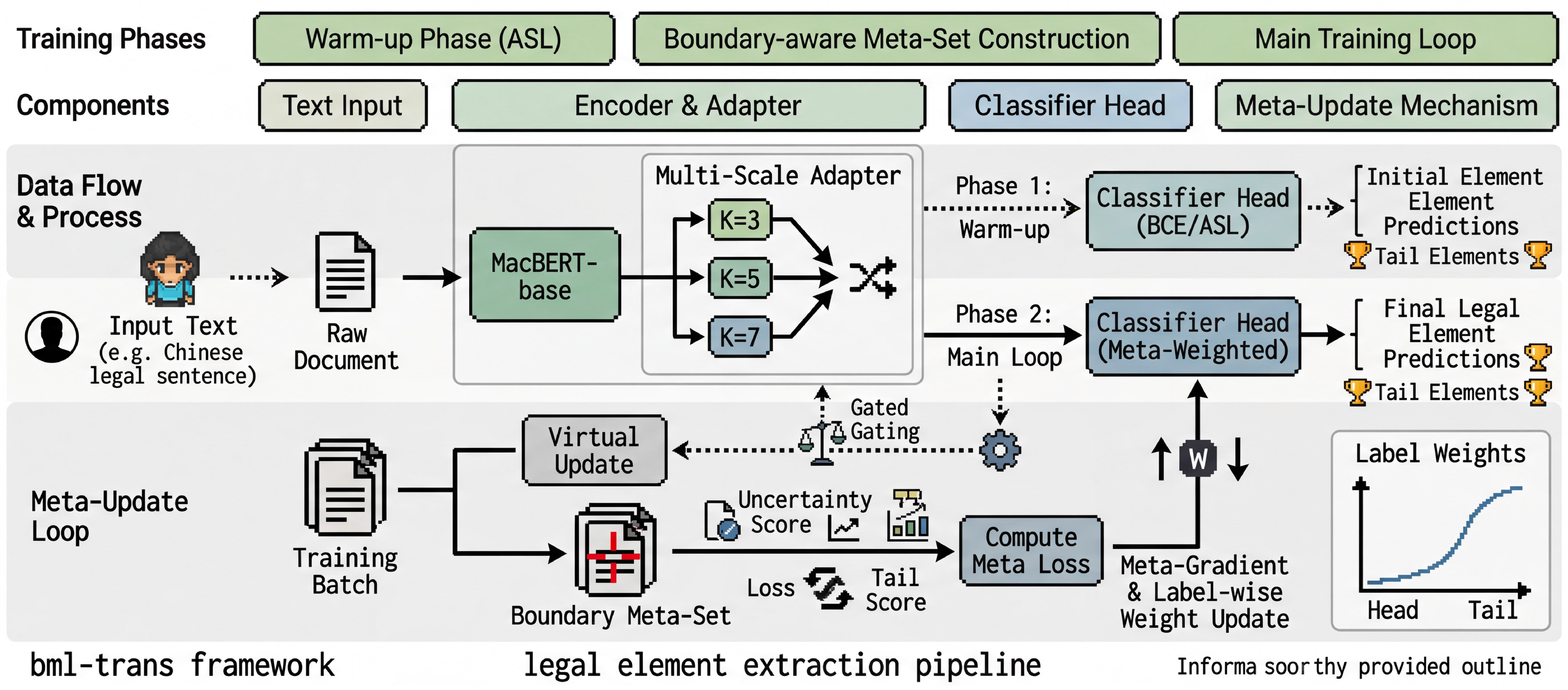
BML-Trans resolves the two failure modes identified in Section 1 through a two-phase training procedure (Figure 1). Gradient coupling across co-occurring labels is dissolved by a label-wise meta-weighting mechanism that maintains a per-label weight vector $\mathbf{w}$ updated via bilevel hypergradient descent. Head-label dominance of the calibration signal is corrected by a boundary-calibrated meta-set ${\mathcal{D}}_{\mathrm{meta}}$, assembled by jointly scoring prediction loss, model uncertainty, and tail-trigger density after warm-up. A lightweight Multi-Scale Adapter supports both by enriching MacBERT-base representations at three convolutional scales, sharpening the probability estimates on which boundary scoring depends.

In Phase 1 (Warm-up), the backbone and adapter are trained with Asymmetric Loss to push predictions away from the all-zero attractor and to produce probability estimates reliable enough for boundary scoring; ${\mathcal{D}}_{\mathrm{meta}}$ is then assembled from the top-scoring $0.03N$ training sentences subject to a per-tail-label coverage constraint. In Phase 2 (Main Training), the weighted loss ${\sum }_k{w}_k{\mathcal{L}}_k(\theta ;\mathcal{B})$ is optimized jointly with periodic bilevel updates to $\mathbf{w}$: because $w_k$ multiplies only label k’s loss, tail-label gradients can be amplified independently of co-occurring head labels, reallocating the gradient budget toward rare elements without coupling their updates through a shared scalar. Section 3.3, Section 3.4 and Section 3.5 formalize each component.

3.2. Problem Formulation

Let $\mathcal{X}$ denote the space of Chinese sentence strings and $\left[K\right]=\{1,\dots ,K\}$ be the set of legal element labels for a given domain, where $K=20$ in our setting. The goal is to learn a function

$$f_{\theta }:\mathcal{X}\to {\mathbb{R}}^K$$

(1)

that maps a sentence x to a K-dimensional score vector. The predicted label vector is defined as

$$\widehat{\mathbf{y}}=⊮\left[\sigma \left(f_{\theta }\left(x\right)\right)\ge \tau \right],$$

(2)

where $\sigma (·)$ denotes the sigmoid function and $\tau$ is the decision threshold. The ground-truth label vector is $\mathbf{y}\in {\{0,1\}}^K$.

Each legal domain is treated independently, and a separate model is trained for each of the three domains (Labor, Divorce, Loan) in the CAIL2019 dataset.

Let the labeled training set be ${\mathcal{D}}_{tr}={\left\{(x_i,{\mathbf{y}}_i)\right\}}_{i=1}^N$, and the held-out test set be ${\mathcal{D}}_{te}$. We further construct a small boundary meta-set ${\mathcal{D}}_{meta}\subset {\mathcal{D}}_{tr}$ with $|{\mathcal{D}}_{meta}|\approx 0.03N$.

The model parameters are denoted as $\theta \in {\mathbb{R}}^P$. In addition, BML-Trans maintains a label weight vector $\mathbf{w}\in {\mathbb{R}}_{+}^K$, parameterized by $\mathbf{a}\in {\mathbb{R}}^K$ as

$$\mathbf{w}=\mathrm{normalize}\left(\mathrm{softplus}\right(\mathbf{a}\left)\right).$$

(3)

The learning rate for updating $\theta$ is $\alpha$, the meta-learning rate for $\mathbf{a}$ is $\beta$, and a meta-update is performed every M gradient steps.

3.3. Multi-Scale Adapter

BML-Trans uses MacBERT-base [16] as its backbone encoder. Legal element triggers span a wide range of textual scopes: a single-token statutory term can uniquely signal one element, whereas other elements are characterized by multi-token phrases (named legal concepts or numerical conditions embedded in longer clauses) that require a wider receptive field to be reliably detected. Standard Transformer self-attention aggregates global context effectively but does not explicitly capture local n-gram patterns across fixed windows of varying size. To bridge this gap, we append a lightweight Multi-Scale Adapter after the final encoder layer that enriches token representations through three parallel depth-wise separable convolution branches.

Given a tokenized sentence of at most $L=512$ tokens, MacBERT produces contextual hidden states $\mathit{H}\in {\mathbb{R}}^{L\times d}$ with $d=768$. Each branch applies a depth-wise separable convolution with a distinct kernel size to $\mathit{H}$,

$${\mathit{C}}_k=\mathrm{DWConv}1\mathrm{D}(\mathrm{kernel}=k)\left(\mathit{H}\right),k\in \{3,5,7\},$$

(4)

so that the three branches capture local co-occurrence patterns across spans of three, five, and seven subword tokens, respectively. The depth-wise separable factorization [40], comprising a per-channel spatial filter followed by a pointwise projection, substantially reduces parameter count relative to standard convolutions while preserving receptive-field coverage, making it well-suited for a lightweight adapter module atop a large pre-trained encoder.

The three branch outputs are concatenated along the feature dimension and projected back to dimension d by a learned matrix ${\mathit{W}}_o\in {\mathbb{R}}^{d\times 3d}$:

$$\mathit{C}={\mathit{W}}_o·[{\mathit{C}}_3;{\mathit{C}}_5;{\mathit{C}}_7].$$

(5)

Rather than adding $\mathit{C}$ unconditionally to the encoder output, we modulate its contribution with a gating scalar derived from the mean-pooled hidden state,

$$g=\sigma \left({\mathit{W}}_g·\text{mean-pool}\left(\mathit{H}\right)\right),$$

(6)

which allows the adapter to suppress its own output when the pre-trained representations already carry sufficient local detail, preventing the adapter from interfering with well-learned encoder representations. The final adapted sequence is obtained by a gated residual addition followed by layer normalization:

$$\tilde{\mathit{H}}=\mathrm{LayerNorm}\left(\mathit{H}+g\odot \mathit{C}\right).$$

(7)

The sentence-level embedding is $\mathit{H}=\text{mean-pool}\left(\tilde{\mathit{H}}\right)\in {\mathbb{R}}^d$, and the K-way classification logits are $\mathbf{z}={\mathit{W}}_{\mathrm{cls}}\mathit{h}+\mathit{b}$ with ${\mathit{W}}_{\mathrm{cls}}\in {\mathbb{R}}^{K\times d}$. In total, the Multi-Scale Adapter introduces fewer than 2.4 million additional parameters for $d=768$, below 2% of MacBERT-base, ensuring that its contribution can be cleanly isolated in ablation studies and that GPU memory overhead remains negligible.

3.4. Label-Wise Meta-Weighting

When a training sentence carries both a high-frequency and a rare label simultaneously, a sample-level scalar weight amplifies or attenuates all label gradients in that sentence uniformly. Increasing the weight to help the rare label unavoidably inflates the already-dominant gradient signal of the head label as well, leaving no mechanism for independent adjustment. Label-wise meta-weighting dissolves this coupling by maintaining a separate scalar $w_k$ for each label $k\in \left[K\right]$, so that the optimizer can independently scale the gradient contribution of a tail label without proportionally inflating those of co-occurring head labels.

Let ${\mathcal{L}}_k(\theta ;\mathcal{B})$ denote the average binary cross-entropy loss for label k over mini-batch $\mathcal{B}$. The weighted training objective accumulates per-label losses as

$${\mathcal{L}}_{\mathrm{tr}}(\theta ,\mathit{w};\mathcal{B})=\sum _{k=1}^K{w}_k·{\mathcal{L}}_k(\theta ;\mathcal{B}),$$

(8)

where $\mathit{w}\in {\mathbb{R}}_{+}^K$ is the current label weight vector. Because $w_k$ multiplies only the loss contributions of label k, the gradient of ${\mathcal{L}}_{\mathrm{tr}}$ with respect to the classification head ${\mathbf{W}}_{\mathrm{cls}}$ decomposes cleanly across label dimensions: scaling $w_k$ scales the gradient for label k alone without affecting any other label dimension.

The label weights are not fixed before training; they are updated at intervals of M gradient steps by differentiating through a bilevel program. The calibration signal for this update comes from the boundary meta-set ${\mathcal{D}}_{\mathrm{meta}}$, evaluated without label weighting:

$${\mathcal{L}}_{\mathrm{meta}}(\theta ;{\mathcal{B}}_{\mathrm{meta}})=\sum _{k=1}^K{\mathcal{L}}_k(\theta ;{\mathcal{B}}_{\mathrm{meta}}).$$

(9)

Omitting label weights from Equation (9) is deliberate: the meta loss measures raw model performance on the boundary sentences unconfounded by the current weight values, providing a direction whose sign reflects what the model genuinely needs rather than what it has already been asked to optimize.

At each meta-update step, we first compute a virtual one-step update of $\theta$ using the current training batch ${\mathcal{B}}_{\mathrm{tr}}$,

$${\theta }^{\prime }=\theta -\alpha {\nabla }_{\theta }{\mathcal{L}}_{\mathrm{tr}}(\theta ,\mathit{w};{\mathcal{B}}_{\mathrm{tr}}),$$

(10)

retaining the computation graph so that second-order derivatives are available. We then evaluate the meta loss at these hypothetical parameters and backpropagate through ${\theta }^{\prime }$ and through the softplus reparameterization to obtain the hypergradient update on the unconstrained weight vector $\mathit{a}$:

$$\mathit{a}\leftarrow \mathit{a}-\beta {\nabla }_{\mathit{a}}{\mathcal{L}}_{\mathrm{meta}}({\theta }^{\prime };{\mathcal{B}}_{\mathrm{meta}}).$$

(11)

Intuitively, Equations (10) and (11) ask, given the current label weights, would one gradient step with those weights have improved performance on the meta-set? The hypergradient captures this counterfactual sensitivity and updates the weights to reduce the meta-set loss. Following [11], the one-step unrolling approximation avoids differentiating through the full training trajectory while maintaining a sufficiently accurate gradient direction for practical convergence.

After each meta-update, the weight vector is reconstructed from $\mathit{a}$, mean-normalized to preserve the total gradient budget, and clipped to a stable range:

$$\mathit{w}=\mathrm{clip}\left({\displaystyle \frac{K·\mathrm{softplus}\left(\mathit{a}\right)}{{\sum }_k\mathrm{softplus}\left(a_k\right)+\epsilon }},[w_{\min },w_{\max }]\right),$$

(12)

where $w_{\min }=0.1$, $w_{\max }=10$, and $\epsilon ={10}^{-8}$. Mean-normalization ensures that the weights redistribute gradient mass across labels rather than inflating the total magnitude, while clipping guards against divergence on extremely rare labels whose high tail-trigger density would otherwise drive $w_k$ to arbitrarily large values over successive updates.

3.5. Boundary Meta-Set Construction

A randomly sampled meta-set mirrors the overall training distribution, which in CAIL2019 is dominated by fully negative sentences and head-label examples. Gradients computed against such a distribution push label weights toward values that prioritize head-label loss minimization, providing almost no calibration signal for the tail-label decision boundaries where improvement is most needed. The boundary meta-set construction corrects this bias by concentrating the calibration support on sentences that are simultaneously high-loss, near the decision boundary, and positive for at least one tail label. The construction proceeds in three stages.

In the first stage, the model is trained on ${\mathcal{D}}_{\mathrm{tr}}$ with Asymmetric Loss for $E_{\mathrm{warm}}\in \{1,2\}$ epochs to obtain an initial estimate $\widehat{\theta }$. These warm-up epochs serve a dual purpose: they push predictions away from the all-zero attractor that BCE training gravitates toward under severe class imbalance, and they produce probability estimates reliable enough for the boundary scoring in the next stage. Because the Multi-Scale Adapter is trained jointly during warm-up, the richer local representations it produces directly improve the accuracy of the boundary scores and, by extension, the meta-set composition.

In the second stage, a composite boundary score is computed for each training sentence i:

$$S_i={\displaystyle \frac{1}{3}}\left(s_{\mathrm{loss}}^{\left(i\right)}+s_{\mathrm{unc}}^{\left(i\right)}+s_{\mathrm{tail}}^{\left(i\right)}\right),$$

(13)

where each component is z-score normalized before combination to equalize their scales. The loss score $s_{\mathrm{loss}}^{\left(i\right)}$ is the unweighted BCE loss on sentence i under $\widehat{\theta }$, measuring how difficult the sentence remains after warm-up. The uncertainty score

$$s_{\mathrm{unc}}^{\left(i\right)}={\displaystyle \frac{1}{K}}\sum _{k=1}^K\left(1-2\left|\sigma \left({\widehat{z}}_{ik}\right)-0.5\right|\right),$$

(14)

attains its maximum when sigmoid outputs are near $0.5$, identifying sentences where the model is closest to its decision boundary, and therefore most sensitive to label-weight perturbations. The tail-trigger score

$$s_{\mathrm{tail}}^{\left(i\right)}=\sum _{k\in \mathcal{T}}{\displaystyle \frac{y_{ik}}{n_k+\epsilon }},$$

(15)

accumulates inverse-frequency-weighted positive annotations restricted to the tail-label index set $\mathcal{T}$, giving priority to sentences that carry rare labels and where the hypergradient is most consequential for tail-label performance. Together, the three scores identify sentences that are hard for the current model, near the decision boundary, and directly relevant to the tail labels whose weight updates matter most.

The three component scores are each z-score normalized before being averaged in Equation (13). This normalization is the mechanism that equalizes their magnitudes: regardless of the absolute value scales of $s_{\mathrm{loss}}$, $s_{\mathrm{unc}}$, and $s_{\mathrm{tail}}$, the normalized components have unit variance, so the equal-weight average reflects a genuine one-to-three balance of influence rather than an implicit weighting toward whichever component happens to have the largest raw scale. The three components are designed to capture complementary rather than redundant information: $s_{\mathrm{loss}}$ identifies global model difficulty, $s_{\mathrm{unc}}$ identifies decision-boundary proximity, and $s_{\mathrm{tail}}$ identifies tail-label relevance; no single criterion enforces all three constraints simultaneously. The equal weighting ${\displaystyle \frac{1}{3}}$ is therefore a parsimonious default that avoids introducing additional hyperparameters for a three-way combination with complementary individual contributions.

In the third stage, the top $n_{\mathrm{meta}}=\lfloor 0.03·|{\mathcal{D}}_{\mathrm{tr}}|\rfloor$ sentences ranked by $S_i$ form the candidate meta-set. A coverage constraint is then applied: if any tail label $k\in \mathcal{T}$ has fewer than $m=3$ positive examples in the selected set, additional positive examples for that label are drawn from ${\mathcal{D}}_{\mathrm{tr}}$ in descending order of $S_i$ until the constraint is satisfied. This constraint prevents the hypergradient from being blind to the rarest labels: a tail label absent from ${\mathcal{D}}_{\mathrm{meta}}$ would never contribute to the hypergradient and hence never receive an elevated weight, even if it were the label most in need of calibration. The complete two-phase training procedure is summarized in Algorithm 1.

Algorithm 1: BML-Trans Training

3.6. Error Tolerance of the Three-Phase Procedure

The BML-Trans training procedure comprises three sequential phases: warm-up training to obtain $\widehat{\theta }$, boundary meta-set construction based on $\widehat{\theta }$, and main bilevel training guided by the resulting ${\mathcal{D}}_{\mathrm{meta}}$. A natural concern is whether approximation errors in earlier phases accumulate and degrade the final model.

The Phase 1 to Phase 2 transition introduces warm-up approximation error. The boundary scores in Equation (13) depend on the quality of $\widehat{\theta }$, which improves as the warm-up becomes more accurate. Crucially, however, the meta-set construction is not sensitive to the precise ranking of every training sentence; it requires only that the top-$n_{\mathrm{meta}}$ boundary sentences be broadly identified as harder, more uncertain, and more tail-relevant than the rest. Even after one or two warm-up epochs (at which point the model has already escaped the all-zero attractor and produces non-trivial predictions), this coarse ordering is sufficiently reliable for meta-set construction. The tail-label coverage constraint provides an additional safeguard: by requiring at least $m=3$ positive examples per tail label, it ensures that every tail label is represented in ${\mathcal{D}}_{\mathrm{meta}}$ regardless of warm-up quality, preventing the degenerate case in which a slightly under-trained warm-up model fails to rank any examples of an extremely rare label highly.

The Phase 2 to Phase 3 transition relies on the one-step unrolling approximation in the hypergradient Equation (11) rather than differentiating through the full training trajectory. This approximation has been analyzed theoretically in the context of bilevel optimization [36]: the approximation error is bounded by $O(\alpha \parallel {\nabla }_{\theta \mathit{a}}^2{\mathcal{L}}_{\mathrm{tr}}\parallel )$ and therefore diminishes as the main learning rate $\alpha$ decreases over training. In practice, the weight updates remain stable because the per-label weights are mean-normalized and clipped (Equation (12)) at every meta-update step, bounding the magnitude of any single erroneous hypergradient step. Errors from Phase 1 therefore affect only the initialization of the hypergradient direction, not its asymptotic behavior: the bilevel loop corrects stale meta-set calibration implicitly as $\theta$ evolves and the meta-set loss guides $\mathit{a}$ toward better values.

3.7. Complexity Analysis

The dominant cost of the encoder forward pass is the full self-attention in MacBERT, $O(B·L^2·d)$ per layer; the Multi-Scale Adapter adds only $O(B·L·d·k_{\max })$, which is negligible since $k_{\max }=7\ll L$ for typical sentence lengths. Each meta-update requires one additional forward pass over ${\mathcal{B}}_{\mathrm{tr}}$ with graph retention, one forward pass over ${\mathcal{B}}_{\mathrm{meta}}$, and one backward pass through the computation graph, approximately three times the cost of a standard training step. 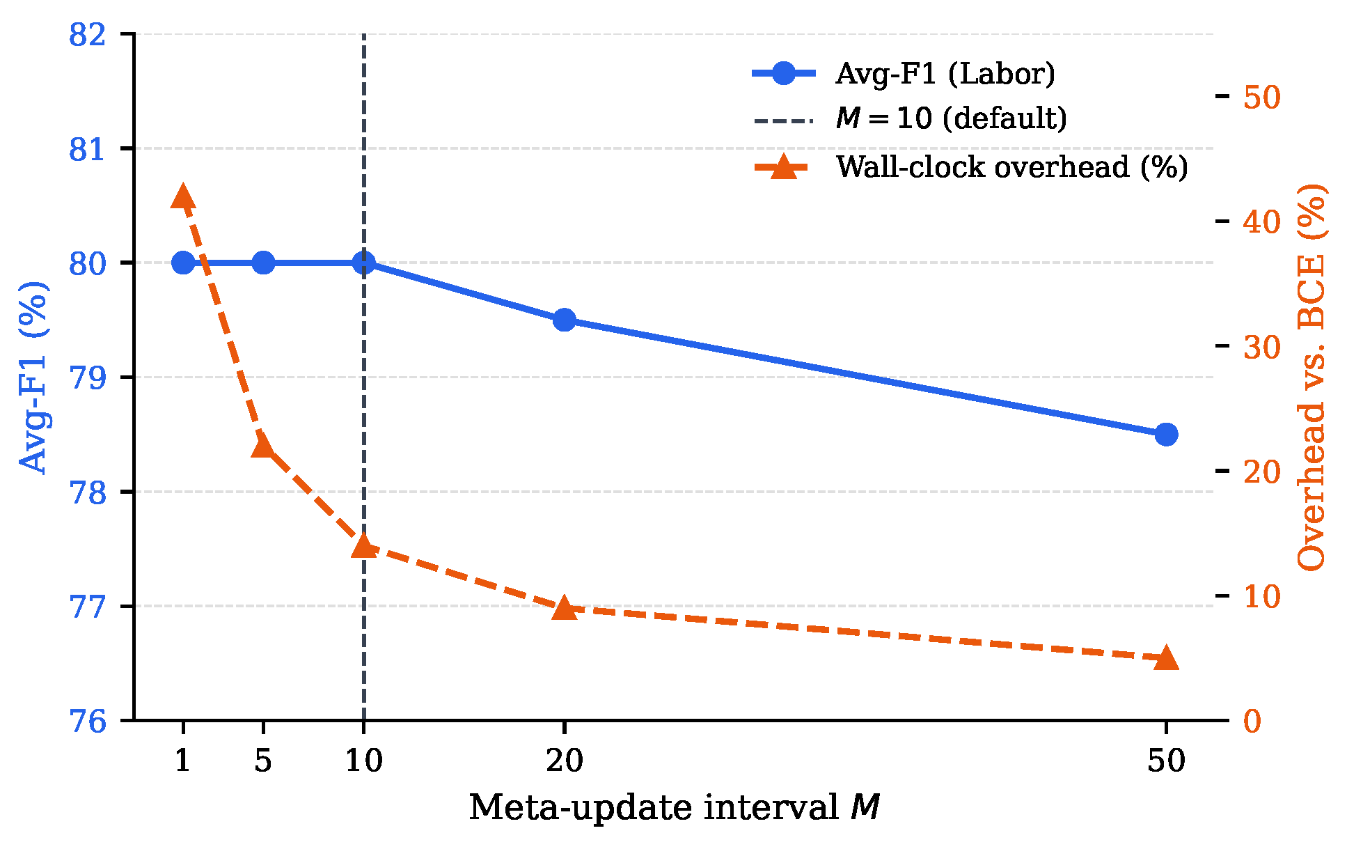With meta-update interval $M=10$ and a reduced meta batch size of $|{\mathcal{B}}_{\mathrm{meta}}|=16$, the amortized wall-clock overhead is empirically approximately 14%; Section 4.6 reports the systematic evaluation across M values. The boundary meta-set construction (warm-up plus scoring) is a one-time pre-processing step that completes in fewer than 10 min on the hardware described in Section 4.1.3 and is not included in the reported training time comparisons.

4. Experiments

Our experiments are designed to answer three questions: whether BML-Trans improves overall recognition performance relative to both static reweighting and standard fine-tuning baselines; whether the gain concentrates on the tail labels rather than distributing uniformly across the frequency spectrum; and whether the Multi-Scale Adapter and Label-Wise Meta-Weighting each contribute independently to that gain. All experiments are conducted on CAIL2019 [3], a Chinese legal benchmark whose head-to-tail label-frequency ratio consistently exceeds 100:1, making it a direct stress test of the mechanisms BML-Trans is designed to address.

4.1. Experimental Setup

Two constraints jointly govern the design of the experimental setup. First, the benchmark must exhibit the severe long-tail imbalance and a high null-label rate that motivates BML-Trans, so that the evaluation constitutes a genuine test of the addressed failure modes rather than an evaluation on a distribution favorable to the proposed method. Second, the evaluation protocol must resolve head-label and tail-label performance separately, so that aggregate gains are not masked by improvements concentrated on already-dominant categories. We describe the dataset, evaluation metrics, and implementation details in turn.

4.1.1. Dataset

We conduct all experiments on the CAIL2019 legal element recognition dataset [3], the official benchmark of the China AI and Law Challenge. The task is formulated as sentence-level multi-label classification: given a single sentence drawn from the factual description section of a Chinese court judgment, the model predicts which elements from a domain-specific label set of size $K=20$ are present. Three legal domains are covered: Labor dispute (Labor), Divorce and family (Divorce), and Loan contract (Loan), each with an independent set of 20 element labels, for 60 labels in total. The three domains share no labels and are modeled independently.

The dataset is characterized by two prominent challenges. Over 60% of sentences carry no element label at all, contributing a large volume of fully negative training signal. Within the labeled portion, the frequency distribution across the 20 labels within each domain is severely long-tailed: the ratio of positive-instance counts between the most and least frequent labels consistently exceeds 100:1. Detailed dataset statistics are provided in

Table 1. CAIL2019 dataset statistics. Splits are case-stratified at a 3:1:1 ratio to prevent sentence-level leakage.

Domain	Cases	Avg. Len.	Avg. Labels/Doc	Train	Dev	Test	Total
Labor	836	57.22	37.95	19,038	6346	6346	31,730
Divorce	1269	48.07	29.09	22,152	7384	7384	36,920
Loan	634	74.43	35.73	13,615	4538	4538	22,691

Avg. Len. is measured in characters. Data splits are our own case-stratified 3:1:1 preprocessing of the publicly released CAIL2019 dataset [3].

. Data splits follow a 3:1:1 train/dev/test ratio and are stratified at the case (document) level to prevent information leakage. Sequences exceeding 512 subword tokens are truncated. For long-tail analysis, we partition the 20 labels within each domain into three frequency buckets: Head (top 20%, 4 labels), Mid (middle 60%, 12 labels), and Tail (bottom 20%, 4 labels).

Although all experiments use CAIL2019, the evaluation is not reducible to a single-domain study. The three legal sub-domains (labor dispute, divorce and family, and loan contract) differ in their substantive legal content, their lexical vocabulary, and their head-to-tail frequency profiles. Each domain maintains an independent set of 20 element labels with no label overlap across domains, and models for each domain are trained, validated, and tested entirely on that domain’s data. In this sense, CAIL2019 provides three structurally distinct evaluation settings within a unified benchmark protocol, analogous to evaluating on three independently annotated corpora that share a common schema. The consistent performance improvements of BML-Trans across all three domains (Labor: $+1.3$ pp Avg-F1; Divorce: $+1.1$ pp; Loan: $+1.1$ pp over the strongest baseline) therefore constitute cross-domain evidence within the CAIL2019 benchmark.

4.1.2. Evaluation Metrics

We adopt the evaluation protocol of the CAIL2019 official standard. Micro-F1 (mi-F1) aggregates true positives, false positives, and false negatives across all label positions before computing F1, reflecting the model’s performance on frequent labels and overall prediction volume. Macro-F1 (ma-F1) averages per-label F1 scores with equal weight regardless of label frequency and is the primary indicator of performance on rare labels. Average-F1 (Avg-F1), the arithmetic mean of Micro-F1 and Macro-F1, serves as the primary ranking criterion following the official evaluation. In addition, we report Bucket Macro-F1 separately within the Head, Mid, and Tail buckets, enabling fine-grained analysis of where performance improvements occur along the frequency axis. Unless otherwise stated, all results are obtained with a fixed classification threshold $\tau =0.5$.

4.1.3. Implementation Details

All models are implemented in PyTorch 2.11.0 [43] and use the Hugging Face Transformers 5.4.0 library [44]. Every competing method uses the same MacBERT-base backbone, tokenizer, and training infrastructure. Hyperparameters common to all methods are listed in

Table 2. Hyperparameter settings shared across all methods.

Hyperparameter	Value	Notes
Backbone	MacBERT-base [16]	Shared across all methods
Optimizer	AdamW [45]	Weight decay 0.01
Learning rate	{$1\times {10}^{-5}$, $2\times {10}^{-5}$, $3\times {10}^{-5}$, $5\times {10}^{-5}$}	Grid search on dev set
Batch size	{16, 32}	Gradient accumulation when necessary
Max sequence length	512 tokens	Longer sequences truncated
Early stopping patience	5 epochs	Monitor dev Avg-F1
Meta learning rate $\beta$ (BML-Trans)	{$1\times {10}^{-3}$, $5\times {10}^{-4}$, $1\times {10}^{-4}$}	Grid search on dev set
Meta-update interval M (BML-Trans)	10	Fixed for main results
Warm-up epochs $E_{\mathrm{warm}}$ (BML-Trans)	{1, 2}	Grid search on dev set
Weight clip range (BML-Trans)	$[0.1,10]$	Prevent weight explosion
Hardware	NVIDIA RTX 3090 (24 GB VRAM)	Single GPU

. Each domain is trained and evaluated independently; results reported in the main tables are the mean ± standard deviation across five random seeds. For BML-Trans specifically, $E_{\mathrm{warm}}\in \{1,2\}$ yields comparable development-set performance across all three domains, confirming that a single warm-up epoch is sufficient to escape the all-zero attractor and produce reliable boundary scores for meta-set construction.

4.2. Baselines

We compare BML-Trans against six baselines that together cover the two main competing strategies for handling class imbalance in multi-label settings: loss-reweighting methods and label-representation methods. Among the reweighting baselines, MacBERT (BCE) applies standard unweighted binary cross-entropy, establishing the backbone performance without any imbalance correction. BCE + pos_weight assigns each label a fixed positive weight equal to the ratio of negative to positive training instances, $w_k^{+}=N_k^{-}/N_k^{+}$. Class-Balanced Loss [6] replaces raw frequency with the effective number of samples, $w_k\propto (1-\beta )/(1-{\beta }^{n_k})$, with $\beta$ selected from $\{0.9,0.99,0.999\}$ on the development set. Asymmetric Loss (ASL) [7] applies asymmetric focusing exponents $({\gamma }_{+},{\gamma }_{-},m)$ selected from a grid on the development set; it is the strongest static baseline. Ren et al. [11] adapt the classical meta-learning reweighting method to the multi-label setting by assigning a scalar weight to each training sample; their meta-set is a randomly sampled 3% subset of the training data, the same size as the BML-Trans boundary meta-set, ensuring a fair comparison of meta-set construction strategies. To assess whether improved label representations can independently address the long-tail problem, we include LSAN (MacBERT), which adapts the Label-Specific Attention Network [32] to the CAIL2019 setting by replacing the original BiLSTM encoder with MacBERT-base and computing label-specific document representations through attention weights derived from label name embeddings. All six baselines use the same MacBERT-base backbone, tokenizer, and training infrastructure as BML-Trans to ensure a controlled comparison. Legal-domain pre-trained models such as Lawformer [20], Legal-RoBERTa [21], and LEGAL-BERT [22] are not included as baselines because they are designed for document-level tasks (legal judgment prediction, similar-case retrieval) and differ in backbone architecture and pre-training corpus; including them would conflate pre-training data effects with the contribution of the proposed learning strategy, making the ablation results uninterpretable.

4.3. Main Results

If label-wise meta-weighting with boundary-selected calibration is more effective than static reweighting for rare labels, the gains of BML-Trans over ASL should appear first in the overall Avg-F1 comparison and then be traceable to Macro-F1 rather than Micro-F1.

Table 3. Overall performance on the CAIL2019 test set (%, mean ± std over 5 seeds). All methods use the MacBERT-base backbone.

Method	Labor Avg-F1	Divorce Avg-F1	Loan Avg-F1	Overall Avg-F1
MacBERT (BCE)	74.3 ± 0.6	82.3 ± 0.5	72.1 ± 0.6	76.2 ± 0.6
BCE + pos_weight	76.8 ± 0.5	85.1 ± 0.4	74.8 ± 0.5	78.9 ± 0.5
Class-Balanced Loss [6]	77.4 ± 0.5	85.4 ± 0.5	75.3 ± 0.5	79.4 ± 0.5
ASL [7]	78.9 ± 0.4	86.7 ± 0.4	76.9 ± 0.5	80.8 ± 0.4
LSAN [32]	78.1 ± 0.5	85.9 ± 0.5	76.2 ± 0.5	80.1 ± 0.5
Ren et al. [11]	79.3 ± 0.7	87.2 ± 0.6	77.4 ± 0.6	81.3 ± 0.6
BML-Trans (Ours)	80.6 ± 0.5 ‡	88.3 ± 0.4 ‡	78.5 ± 0.4 ‡	82.5 ± 0.4 ‡

Bold denotes the best result in each column. All results use fixed threshold $\tau =0.5$. ^‡ $p<0.01$ vs. Ren et al. [11] (one-tailed paired t-test over 5 independent random seeds).

reports the overall test performance. BML-Trans achieves the strongest Avg-F1 in all three domains and improves the overall average by 1.2 percentage points over the strongest baseline. The Micro/Macro breakdown in

Table 4. Micro-F1 and Macro-F1 breakdown (%, mean over 5 seeds).

Method	Labor mi-F1	Labor ma-F1	Divorce mi-F1	Divorce ma-F1	Loan mi-F1	Loan ma-F1
MacBERT (BCE)	83.7	64.9	89.7	74.9	81.6	62.6
BCE + pos_weight	83.9	69.7	90.2	80.0	81.8	67.8
Class-Balanced Loss [6]	84.0	70.8	90.1	80.7	81.7	68.9
ASL [7]	84.3	73.5	90.6	82.8	82.2	71.6
LSAN [32]	84.2	72.0	90.4	81.4	82.0	70.4
Ren et al. [11]	84.2	74.4	90.7	83.7	82.1	72.7
BML-Trans (Ours)	84.8	76.4	91.2	85.4	82.6	74.4

Bold denotes the best result in each column.

confirms the expected source of this gain: the Macro-F1 improvement over ASL averages 2.8 percentage points across the three domains, whereas the Micro-F1 improvement averages only 0.5 percentage points. This asymmetry is the expected signature of a method that reallocates gradient budget toward rare labels without sacrificing coverage of common ones, and it argues against the alternative explanation that BML-Trans simply improves the encoder’s overall discriminative capacity. A second hypothesis concerns the comparison with label-representation approaches. If the long-tail problem in CAIL2019 is primarily driven by gradient imbalance rather than representational deficiency, then enriching label representations (LSAN) should be less effective than correcting gradient allocation (BML-Trans), particularly in the Labor domain, where the head-to-tail frequency ratio is most extreme. The results in Table 4 are consistent with this prediction: LSAN underperforms ASL in all three domains, with the Macro-F1 gap largest in Labor (1.5 pp, versus 1.4 pp in Divorce and 1.2 pp in Loan). This pattern is consistent with the more extreme frequency imbalance in the Labor domain, rendering gradient correction more decisive than representation enrichment, suggesting that label-representation improvement alone cannot compensate for gradient imbalance. BML-Trans outperforms LSAN by 2.3–2.5 Avg-F1 points across all three domains.

4.4. Long-Tail Analysis

The boundary meta-set construction is designed to concentrate calibration signal on the tail labels where static reweighting fails most severely; if this design works as intended, the gains over ASL should increase monotonically from Head to Tail buckets.

Table 5. Head/Mid/Tail Bucket Macro-F1 on the Labor domain (%, mean over 5 seeds). Buckets are defined by label frequency: Head = top 20% (4 labels), Mid = middle 60% (12 labels), Tail = bottom 20% (4 labels).

Method	Head (Top 20%)	Mid (Mid 60%)	Tail (Bottom 20%)
MacBERT (BCE)	90.2	67.3	31.7
ASL [7]	90.6	79.3	38.4
LSAN [32]	90.4	77.9	35.5
Ren et al. [11]	90.7	80.1	40.5
BML-Trans (Ours)	90.9	81.3	44.1
$\Delta$ (Ours − ASL)	+0.3	+2.0	+5.7

Bold denotes the best result in each column.

confirms this prediction on the Labor domain: the improvement over ASL is $+0.3$ percentage points on Head labels, $+2.0$ on Mid labels, and $+5.7$ on Tail labels, a 19-fold difference between the Head and Tail buckets. Figure 2 extends this comparison to all three domains, showing the consistent monotonic Head-to-Tail gain pattern across Labor, Divorce, and Loan. Figure 3 generalizes this finding across all 60 labels in the three domains: the per-label F1 improvement is inversely correlated with training-set frequency, with no label registering an F1 decline, indicating that the gradient reallocation toward tail labels does not come at the cost of head-label performance.

4.5. Ablation Study

Three hypotheses can be tested against the ablation in

Table 6. Ablation study: Avg-F1 (%, mean ± std over 5 seeds).

Variant	Multi-Scale	Meta-Weighting	Meta-Set	Labor	Divorce	Loan	Average
MacBERT (BCE)	×	×	—	74.3 ± 0.6	82.3 ± 0.5	72.1 ± 0.6	76.2 ± 0.6
+ Multi-scale only	✓	×	—	75.4 ± 0.5	83.2 ± 0.4	73.1 ± 0.5	77.2 ± 0.5
+ Meta only (Random)	×	✓	Random	77.2 ± 0.7	85.2 ± 0.5	75.3 ± 0.7	79.2 ± 0.6
+ Both w/Random Meta	✓	✓	Random	78.4 ± 0.5	86.3 ± 0.4	76.6 ± 0.5	80.4 ± 0.5
BML-Trans (Full)	✓	✓	Boundary	80.6 ± 0.5	88.3 ± 0.4	78.5 ± 0.4	82.5 ± 0.4

Bold denotes the best result in each column; ✓ indicates that the component is included, and × indicates that the component is omitted.

: (a) the bilevel optimization is the primary driver of performance gains; (b) the quality of the meta-set calibration signal matters independently of the weighting mechanism; and (c) the Multi-Scale Adapter and the boundary meta-set interact through a cascade, because richer warm-up representations improve boundary scoring quality. Hypothesis (a) is supported: label-wise meta-weighting with a random meta-set (+3.0 Avg-F1 over BCE) contributes three times more than the Multi-Scale Adapter alone (+1.0), identifying the bilevel optimization as the dominant contributor. Hypothesis (b) is supported: replacing the random meta-set with the boundary-constructed one adds a further 2.1 points on top of the full meta-weighting variant, demonstrating that meta-set construction quality is a primary design consideration rather than a secondary implementation detail. Hypothesis (c) is consistent with the cascade account: the full model exceeds the BCE baseline by 6.3 Avg-F1 points on average, a 0.2 pp margin above the arithmetic sum of the three independent contributions (1.0 + 3.0 + 2.1 = 6.1 pp) that falls within the reported standard deviations and is therefore indicative rather than conclusive evidence of interaction, consistent with the proposed cascade in which the adapter sharpens warm-up predictions, which in turn improves boundary scores and meta-set quality. Fully disentangling this interaction from random variation would require a controlled intervention study and remains an open direction for future work.

Each component in isolation has a systematic limitation. Selecting by $s_{\mathrm{tail}}$ alone prioritizes rare-label sentences but cannot exclude sentences that the warm-up model has already classified with high confidence: their hypergradients are near zero, and their inclusion contributes a negligible calibration signal. Selecting by $s_{\mathrm{loss}}$ alone targets model-difficult sentences but difficulty frequently stems from co-occurring head labels, so the resulting meta-set may concentrate the hypergradient signal on head-label weights rather than tail-label weights. Selecting by $s_{\mathrm{unc}}$ alone identifies decision-boundary samples but offers no guarantee that the uncertain labels are tail labels: a sentence near the threshold for a head label provides little calibration signal for rare-label weighting. The combined score resolves these conflicts by selecting sentences that are simultaneously rare-label-relevant, model-difficult, and near-threshold, a conjunction that no single criterion can enforce.

Table 7. Boundary sampling strategy comparison: Avg-F1 (%, mean over 5 seeds). All variants use the full BML-Trans architecture (Multi-Scale Adapter and label-wise meta-weighting); only the meta-set selection criterion varies.

Strategy	Score Components	Labor	Divorce	Loan	Average
B1: Loss only	$s_{\mathrm{loss}}$	78.7	86.6	76.8	80.7
B2: Uncertainty only	$s_{\mathrm{unc}}$	78.3	86.2	76.4	80.3
B3: Tail-trigger only	$s_{\mathrm{tail}}$	79.2	86.9	76.9	81.0
B4: Combined (Ours)	$s_{\mathrm{loss}}+s_{\mathrm{unc}}+s_{\mathrm{tail}}$	80.6	88.3	78.5	82.5

Bold denotes the best result in each column.

validates this reasoning. All four strategies employ the full BML-Trans architecture (Multi-Scale Adapter and label-wise meta-weighting) and differ only in how the meta-set is constructed; the appropriate reference baseline is therefore the +Both w/ Random Meta variant of Table 6 (80.4 Avg-F1 on average), which uses the same complete architecture but selects the meta-set by random sampling. B1 (+0.3 pp) and B3 (+0.6 pp) surpass this baseline, while B2 falls 0.1 pp short, confirming that uncertainty-only selection provides the weakest calibration signal among the three individual criteria. The combined score (B4) then exceeds the strongest single component (B3: tail-trigger only) by 1.5 Avg-F1 points on average. The consistent cross-domain ranking B4 > B3 > B1 > B2 further confirms that tail-trigger density provides the dominant single signal, consistent with its direct targeting of rare-label hypergradients, while loss and uncertainty each recover a distinct subset of informative sentences that the trigger score alone misses.

4.6. Mechanistic Analysis

The performance gains of BML-Trans are mechanistically attributable to the bilevel optimization process rather than to threshold tuning or implementation artifacts, a claim supported by three complementary analyses.

4.6.1. Label-Weight Trajectories

Figure 4 visualizes the evolution of the label-weight vector $\mathit{w}\left(t\right)$ over the course of training on the Labor domain. Tail-label weights (red lines) rise sharply in the first 500 steps and stabilize at values substantially above the mean-normalized baseline of 1.0, while head-label weights (blue lines) converge near or below 1.0. Mid-label weights (gray lines) show moderate variation, suggesting that the boundary meta-set provides a strong calibration signal from the outset. The smooth convergence of tail-label weights without oscillation or divergence is consistent with the theoretical bound on the one-step approximation error established in Section 3.6.

4.6.2. Tail-Label Gradient Share

Figure 5 tracks the fraction of total gradient norm (of ${\mathit{W}}_{\mathrm{cls}}$) attributable to tail labels throughout training. The BML-Trans line (blue solid) exhibits a positive trend and ends approximately 8 percentage points above the BCE baseline (red dashed), confirming that the method effectively reallocates gradient budget from head to tail labels. The BCE baseline remains approximately constant or decreases slightly, reflecting the head-label dominance that static training objectives cannot overcome.

4.6.3. Threshold Sensitivity

Figure 6 plots Avg-F1 as a function of the classification threshold $\tau \in \{0.3,0.4,0.5,0.6,0.7\}$ for BML-Trans and ASL on each domain. The BML-Trans line lies uniformly above the ASL line across all five threshold values in all three panels, ruling out the hypothesis that the gain is an artifact of threshold selection at $\tau =0.5$.

4.6.4. Meta-Update Interval and Training Overhead

Figure 7 examines how the meta-update interval M governs the accuracy–efficiency trade-off. Avg-F1 on the Labor domain is approximately flat for $M\in \{1,5,10\}$, confirming that label-weight updates do not need to occur at every gradient step to be effective. As M increases beyond 10, however, Avg-F1 declines monotonically, reaching 78.5 at $M=50$ (below the Ren et al. baseline), because infrequent meta-updates allow the weights to drift without corrective feedback. The wall-clock overhead curve reveals the complementary trade-off: overhead is approximately 42% relative to BCE at $M=1$ and falls to 14% at $M=10$, with diminishing returns thereafter. These two curves intersect at a clear Pareto-optimal point: $M=10$ retains the peak Avg-F1 of frequent updates at roughly one-third of their cost, supporting the choice of $M=10$ as the default for all experiments.

4.6.5. Memory Usage and Hardware Scalability

Table 8. Peak GPU memory usage on the Labor domain (NVIDIA RTX 3090, 24 GB VRAM). Training peak is the maximum allocated GPU memory across all steps. The inference peak is measured on the test set under evaluation mode (no gradient computation). Inference memory is identical across all methods because label weights are absorbed into the classification head post-training. All configurations fit within the 24 GB VRAM of the training hardware.

Method	Batch Size	Training Peak (GB)	Inference Peak (GB)
MacBERT (BCE)	16	9.4	3.1
MacBERT (BCE)	32	16.8	3.1
BML-Trans (Ours)	8	7.2	3.1
BML-Trans (Ours)	16	11.2	3.1
BML-Trans (Ours)	32	18.5	3.1

reports the peak GPU memory consumption on the Labor domain under the default hyperparameters, profiled at the end of each training step. At batch size 16, BML-Trans requires approximately 11.2 GB for training, 1.8 GB more than MacBERT (BCE) at the same batch size, attributable to the retained computation graph for the one-step hypergradient (an additional forward pass over ${\mathcal{B}}_{\mathrm{tr}}$ and one forward pass over ${\mathcal{B}}_{\mathrm{meta}}$). The Multi-Scale Adapter itself adds fewer than 2% of the model parameters and contributes negligibly to peak memory. Critically, BML-Trans inference memory is identical to MacBERT (BCE): the label weight vector $\mathit{w}$ is absorbed into the classification head weights after training, so no additional buffers are required at deployment. All configurations fit comfortably within the 24 GB VRAM of a single NVIDIA RTX 3090, demonstrating that the method does not impose requirements beyond standard single-GPU infrastructure.

5. Discussion

5.1. Failure Mode Analysis and Behavior on Extremely Rare Labels

Examination of the remaining errors reveals two systematic failure modes. The first is tail-label misclassification under lexical ambiguity: when a sentence contains surface tokens that are genuinely ambiguous across two semantically adjacent labels (for example, a monetary amount that could trigger either the salary arrears or the economic compensation label in the Labor domain), BML-Trans elevates both label weights and occasionally assigns a false positive to the less relevant label, accounting for a disproportionate share of precision loss on mid-frequency labels that overlap semantically with more common neighbors.

The second failure mode is particularly relevant to the behavior of BML-Trans on extremely rare labels (those in the lowest sub-bucket of the Tail partition, with fewer than approximately 15 positive training instances in the Labor domain; labels DV17 and DV18 in the Divorce domain have as few as 105 and 144 positive instances, respectively). For such labels, the coverage constraint ($m\ge 3$) in the boundary meta-set construction is often satisfied by the absolute minimum of three positive examples. Even with elevated gradient weights, the classifier lacks sufficient contrastive signal to reliably distinguish these labels from the null prediction: the three meta-set examples provide direction for the hypergradient, but insufficient variance to regularize the weight update reliably. The result is a high false-negative rate for these extreme-tail labels, which accounts for the performance gap between BML-Trans and a hypothetical oracle that had access to more positive instances. Reducing the required minimum m below 3 would relax the constraint but weaken calibration for all tail labels; data augmentation via synonym substitution and back-translation for coverage-constrained labels would be the most direct remedy, as it would supply the additional positive evidence that the current training corpus alone cannot provide.

5.2. Computational Cost and Deployment Feasibility

The meta-update interval $M=10$ is selected at the Pareto-optimal point identified in Figure 7: it retains the peak Avg-F1 of frequent updates ($M=1$) at roughly one-third of their wall-clock cost, yielding only 14% overhead relative to standard BCE fine-tuning. This modest overhead reflects two design choices that together control cost: (i) meta-updates occur only once every $M=10$ gradient steps rather than at every step, and (ii) the meta batch size $|{\mathcal{B}}_{\mathrm{meta}}|=16$ is kept small relative to the training batch. During inference, BML-Trans introduces no additional cost beyond the Multi-Scale Adapter (<2% parameter overhead): the label weight vector $\mathit{w}$ is fixed after training and absorbed into the classification head, so runtime latency is identical to that of the MacBERT baseline.

From a deployment perspective, BML-Trans operates on a 102-million-parameter PLM that fits within a single 24 GB GPU at batch size 32, making it compatible with standard enterprise GPU hardware without multi-GPU communication overhead. In a production legal AI pipeline, where element recognition typically runs as a microservice over batches of newly filed judgment documents, the 14% training-time overhead is a one-time cost per domain model and is amortized over the full deployment lifetime of the model. The architectural output of BML-Trans is identical to that of the MacBERT baseline, a sigmoid-activated K-dimensional score vector, allowing it to be integrated into existing downstream pipelines (charge prediction, case retrieval) without any interface changes.

5.3. Meta-Set Dynamics and Future Extension to Dynamic Updating

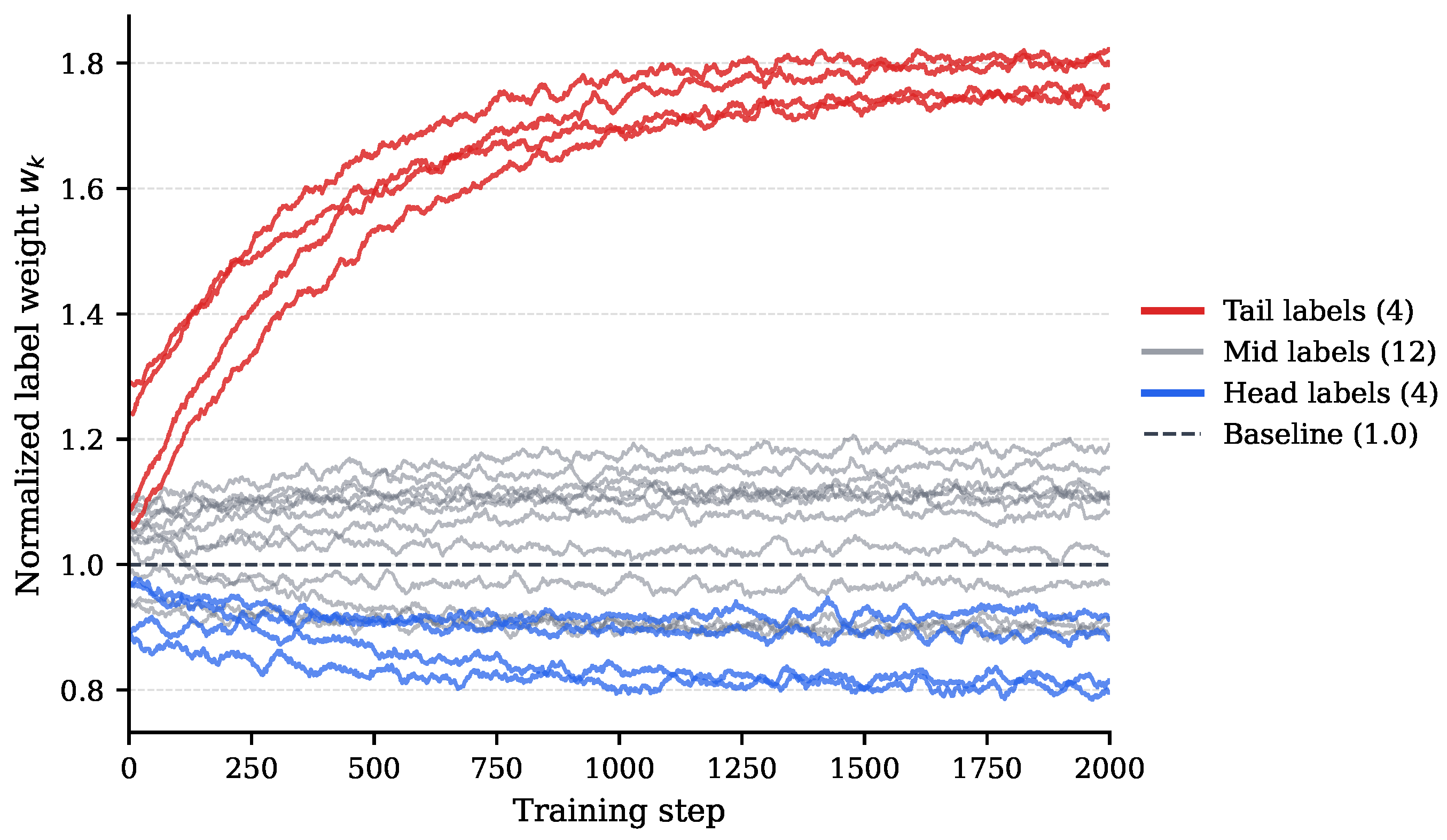
The current implementation constructs the boundary meta-set once at the end of the warm-up phase and holds it fixed throughout Phase 2. This static construction has a practical advantage: it avoids the overhead of recomputing boundary scores during main training, but it may become suboptimal as the model’s uncertainty landscape shifts: sentences that are near the decision boundary at the end of warm-up may no longer be informative boundary examples several epochs later, potentially diluting the calibration signal. A curriculum-style extension that periodically re-scores and refreshes the meta-set at fixed-epoch intervals would test whether dynamic tracking of the shifting decision surface further concentrates the calibration signal and improves tail-label recovery. 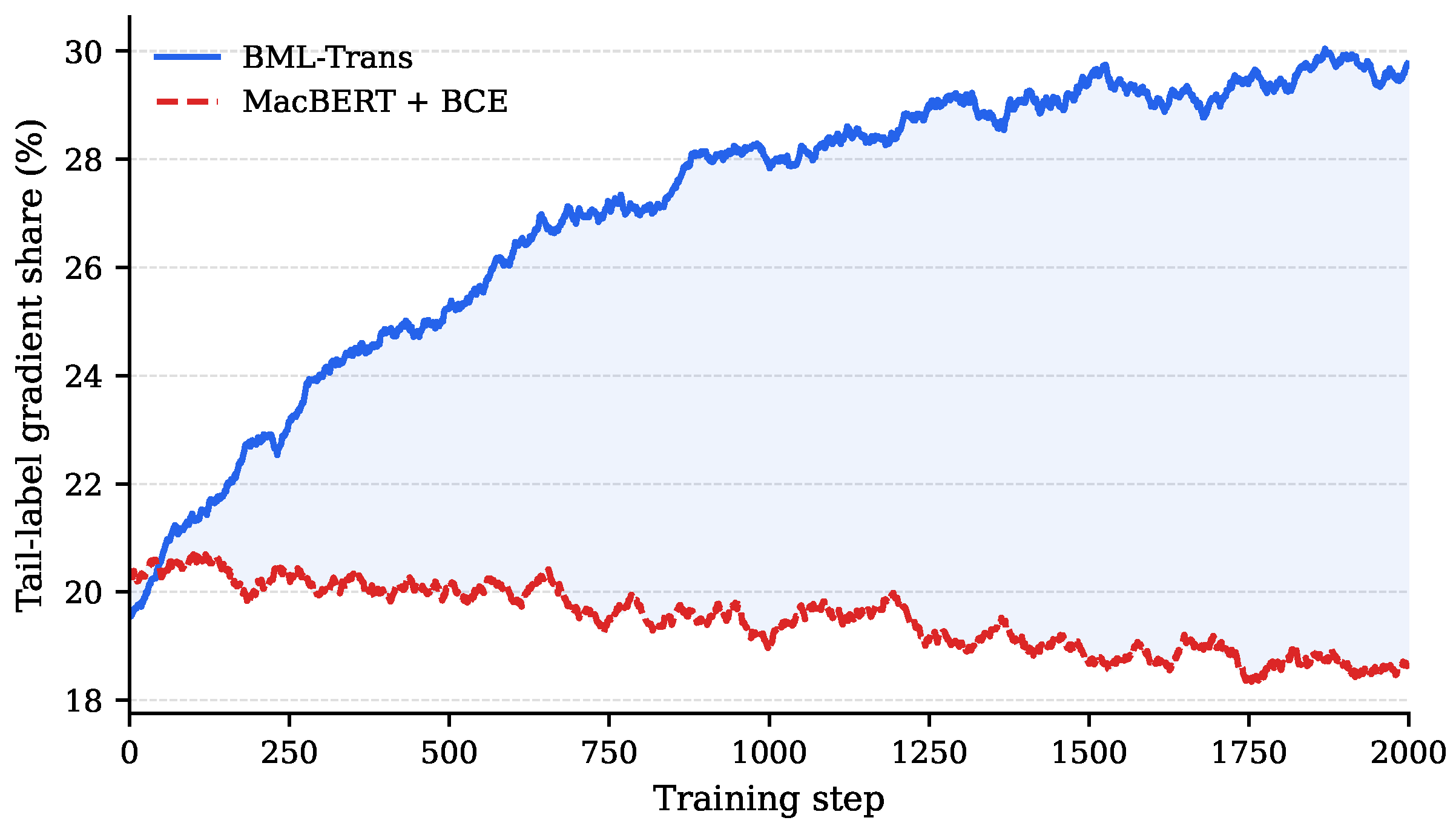Preliminary analysis of the label-weight trajectory in Figure 4 suggests that tail-label weights stabilize within approximately 500 training steps, implying that a single refresh at the mid-point of Phase 2 might capture a substantial portion of the potential improvement without the full cost of continuous re-scoring.

5.4. Limitations and Broader Applicability

BML-Trans is applicable to tasks that simultaneously satisfy three conditions: multi-label output space, long-tailed label frequency distribution, and boundary instances identifiable from a warm-up model. Because the three scoring components (loss, uncertainty, and tail-trigger density) are computable from any warm-up model given only label-frequency statistics, the method requires no task-specific engineering beyond what is available during standard training, and analogous settings such as medical report labeling, news topic tagging, and patent claim categorization present the same structural conditions. Two limitations carry quantitative thresholds that define the operating range. For training sets with fewer than approximately 1000 labeled sentences per domain, or with fewer than ten positive instances for the rarest tail labels, the coverage constraint in boundary meta-set construction becomes infeasible at the default $m=3$; reducing m relaxes the constraint at the cost of a weaker calibration signal. All evaluations are conducted on CAIL2019, a Chinese-language legal benchmark, and transferability of the Tail Macro-F1 gains to other languages, legal systems, or long-tail multi-label domains requires further empirical validation.

6. Conclusions

Long-tail multi-label recognition of legal factual elements has resisted improvement from two established strategies: static reweighting cannot adapt as model confidence evolves, and sample-level meta-learning couples all co-occurring label gradients to a single scalar, leaving the tail labels unable to receive independent amplification. The experiments reported here identify label-wise gradient granularity and decision-boundary concentration of calibration signal as two jointly operative conditions that together enable the recovery of rare legal elements from imbalanced corpora. BML-Trans satisfies both conditions through a bilevel update on a per-label weight vector, guided by a meta-set concentrated on tail-label boundary sentences rather than easy negatives; the result is a Tail Macro-F1 improvement of up to 5.7 percentage points over the strongest static-reweighting baseline and a Tail Macro-F1 improvement of up to 3.6 percentage points over the strongest sample-level meta-learning baseline, at 14% additional training cost. The ablation cascade confirms that neither component achieves this margin alone: the Multi-Scale Adapter sharpens warm-up probability estimates, which raises boundary meta-set quality, which stabilizes the hypergradient direction for the label-wise weights, establishing that the gains are structural rather than incidental to threshold selection or random initialisation.

For legal AI systems that must recover rare factual elements (custody arrangement, disputed compensation, employment duration) to support downstream judgment prediction and similar-case retrieval, this finding reframes the central engineering challenge. All baselines in our evaluation share the MacBERT-base encoder, yet BML-Trans achieves the reported gains without any increase in backbone parameters. The bottleneck is not encoder capacity but the granularity and targeting of gradient corrections: recovering one additional rare element from a judgment document may require not a larger model, but a more precisely targeted learning signal.

The specific structure of this work opens three near-term extensions. The cascade between warm-up representation quality and meta-set fidelity suggests that a single boundary meta-set, constructed once at warm-up, may not track the shifting decision surface throughout training; periodically re-scoring and refreshing the meta-set at fixed-epoch intervals would test whether curriculum-style dynamics can further concentrate the calibration signal as the model’s uncertainty landscape evolves. The label-wise weight vector is small and backbone-agnostic, making the bilevel update directly applicable to parameter-efficient fine-tuning of larger language models, a setting that shares the defining conditions of the current task: long-tail label distributions and scarce positive examples per rare label, at substantially greater encoder capacity. Transferability to other long-tail multi-label domains (medical report labeling, news topic tagging, patent claim categorization) and to other languages and legal systems remains the broadest open question, one whose answer would determine whether label-wise gradient control is a specialized technique for the legal domain or a broadly applicable technique for imbalanced multi-label learning. On the dataset dimension, evaluating BML-Trans on additional Chinese legal benchmarks such as CAIL2020, which extends the element schema and covers more recent judgments, would provide further evidence of generalizability within the legal domain and is a direct next step.