Evaluation of a Non-Parametric Penalized Kaplan–Meier Estimator Under Interval-Censored Survival Data


Abstract
1. Introduction
2. Materials and Methods
2.1. Kaplan–Meier Estimator
2.2. Non-Parametric Penalized Kaplan–Meier Estimator
2.3. Imputation Methods for Interval Censoring
2.3.1. Midpoint Imputation
2.3.2. Regression Imputation
- A pseudo-exact time was initially created for each interval-censored observation using the midpoint of .
- The Weibull accelerated failure time (AFT) model was estimated using the survreg() function from the survival package in R. The survreg() function fits parametric survival regression models under the AFT framework by maximizing the full likelihood, accommodating right-, left-, and interval-censored survival data. Specifically, survreg() assumes that the logarithm of the survival time follows a linear regression model with an additive error term whose distribution determines the parametric form of the survival model. For the Weibull specification, the error term is assumed to follow a standard extreme value (Gumbel) distribution, which implies a Weibull distribution for the survival time . Model parameters, including the regression coefficients , the intercept , and the scale parameter , are estimated via maximum likelihood.The Weibull shape parameter is given by and the scale parameter is , linking the AFT parameterization used by survreg() to the conventional Weibull distribution. This flexibility, combined with native support for interval-censored data, makes survreg() well suited for regression-based imputation and survival modeling in interval-censored settings.
- The fitted model produced predicted event timeswhich were then truncated to the subject’s interval:
- In instances where the Weibull AFT model failed to converge, typically due to limited data variability, sparse failures, or instability in the likelihood, the midpoint of the interval was used as a robust fallback imputation:
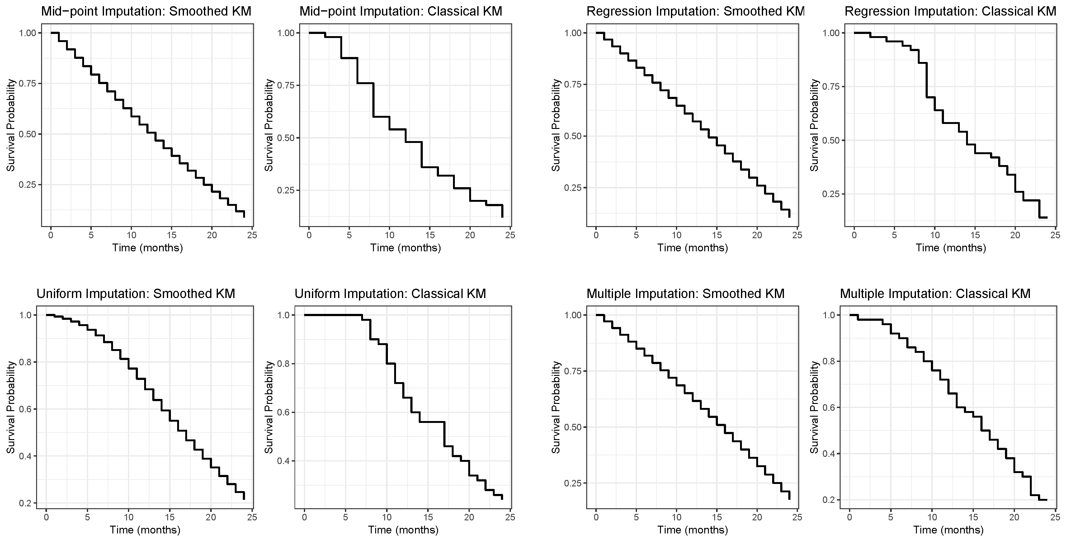
- The final regression imputed times were analyzed using both the classical KM estimator and the smoothed penalized-likelihood KM estimator.
2.3.3. Uniform Imputation
2.3.4. Multiple Imputation
- Generate M independent completed datasets:where each is drawn from an approximation to the posterior predictive distribution
- Fit the desired model separately to each imputed dataset, obtaining point estimates and the corresponding variance estimates .
- Combine M results using Rubin’s rules:where is the pooled point estimate, represents the average within-imputation variance, B represents the between-imputation variance, and T represents the total variance incorporating both within- and between-imputation uncertainty.
2.4. Performance Evaluation Metrics
2.4.1. Mean Absolute Error (MAE)
2.4.2. Normalized Mean Absolute Error (NMAE)
2.4.3. Maximum Absolute Error (MaxAE)
2.4.4. Mean Squared Error (MSE)
2.4.5. Normalized Root Mean Squared Error (NRMSE)
2.4.6. Normalized Average Root Median Error Deviation (NARMED)
3. Results
3.1. Simulation Study
3.1.1. Monte Carlo Simulation Design
3.1.2. Simulation of Interval-Censored Data
- The population size based on a total of observations was initially generated to serve as the source population.
- Random samples of size were drawn from the population in each iteration.
- For each sample size, bootstrap replicates were generated to ensure stability and precision of the performance estimates.
- The different prevalence rates were applied.
3.1.3. Generation of True Survival Estimates
- A population of size was used as the source population from which bootstrap samples were drawn.
- For each bootstrap iteration , with , a random sample of size n was drawn from the population with a replacement.
- For each bootstrap sample and each imputation method, a KM estimator was computed based on the imputed event times.
- To reduce sampling variability and obtain a continuous survival estimate, each KM curve was smoothed using cubic spline interpolation.
- The smoothed survival curves were evaluated on a dense and fixed time grid:
- The final reference (true) survival function was obtained by averaging the smoothed survival estimates across all bootstrap samples:where denotes the smoothed KM survival probability at time t from the bootstrap replicate.
- The resulting averaged survival function was treated as the true survival curve and used as the benchmark for evaluating estimator performance.
3.1.4. Computation of Performance Evaluation Metrics
3.2. Monte Carlo Simulation Results
3.2.1. Descriptive Analysis of Simulated Interval-Censored Data
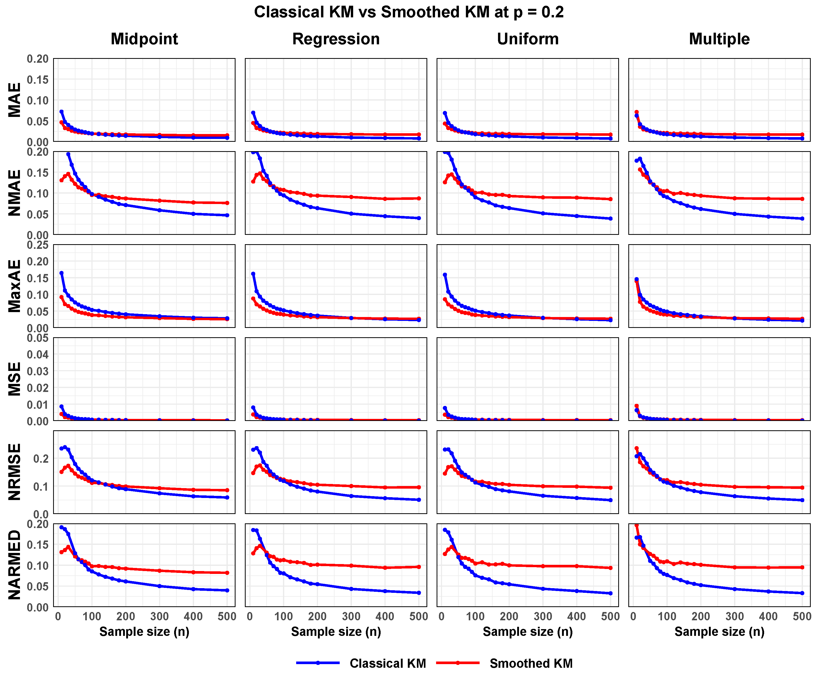
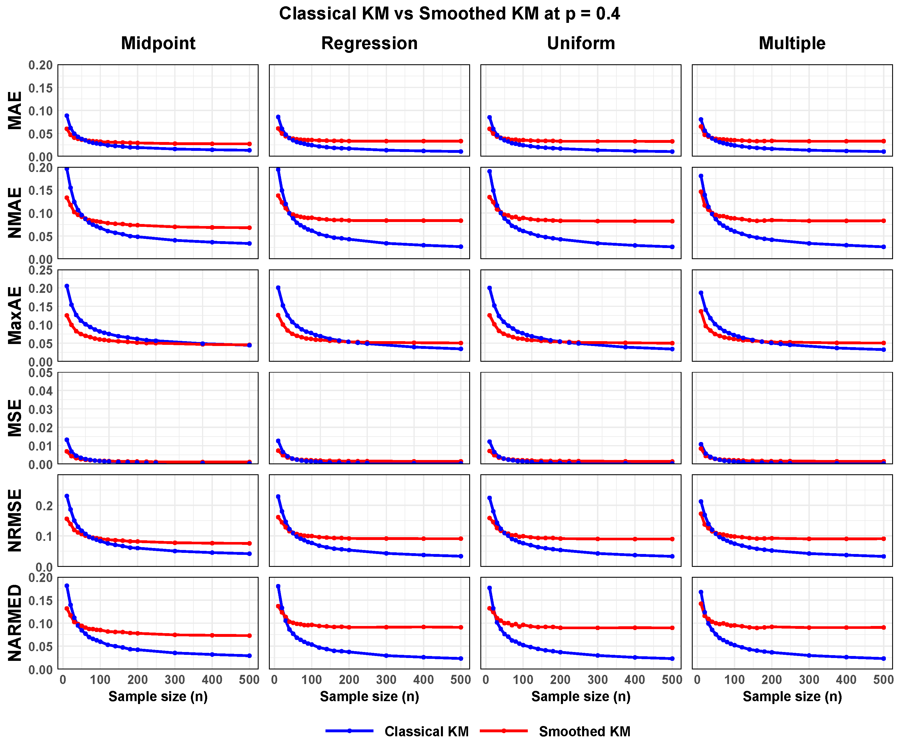
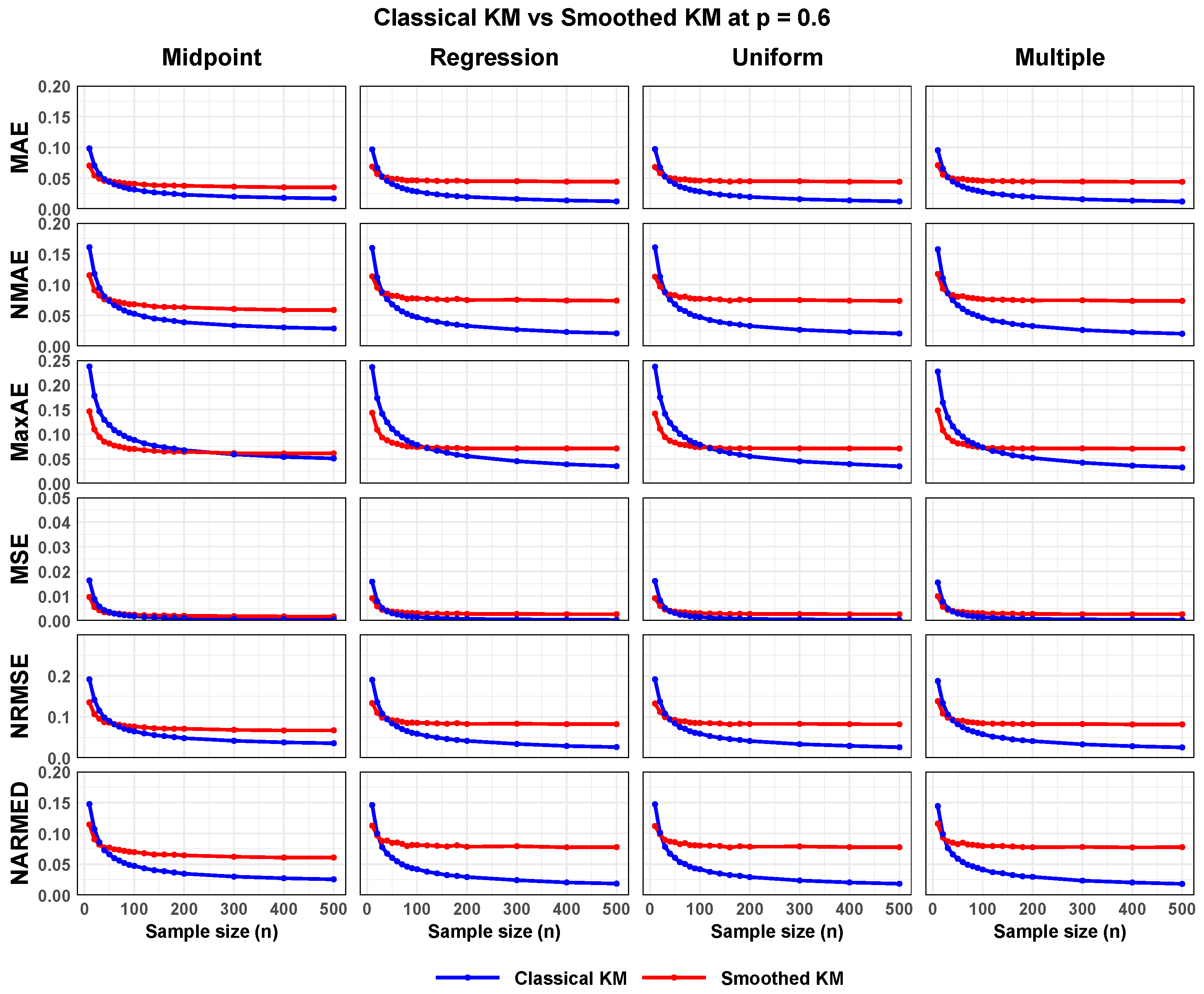
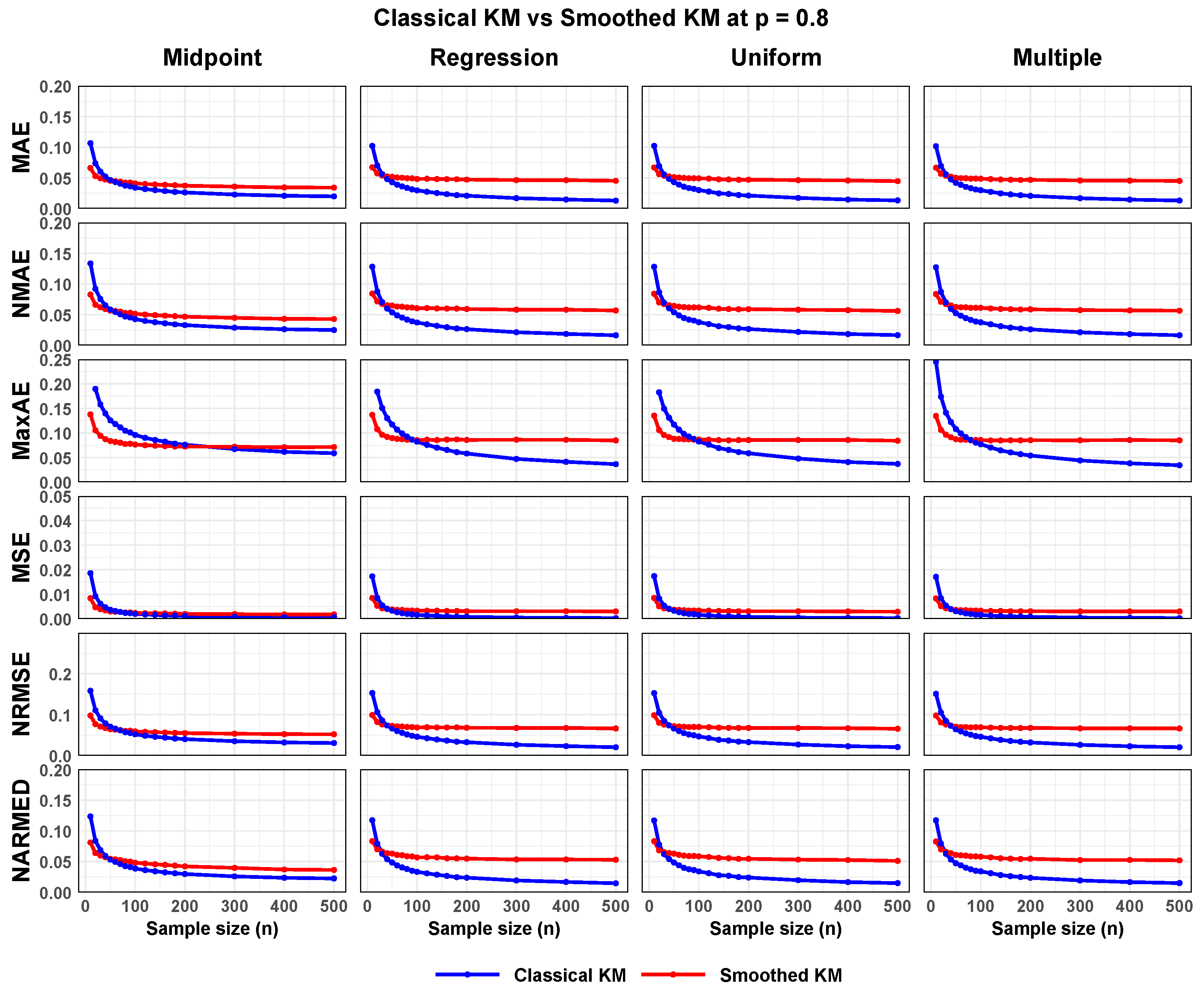
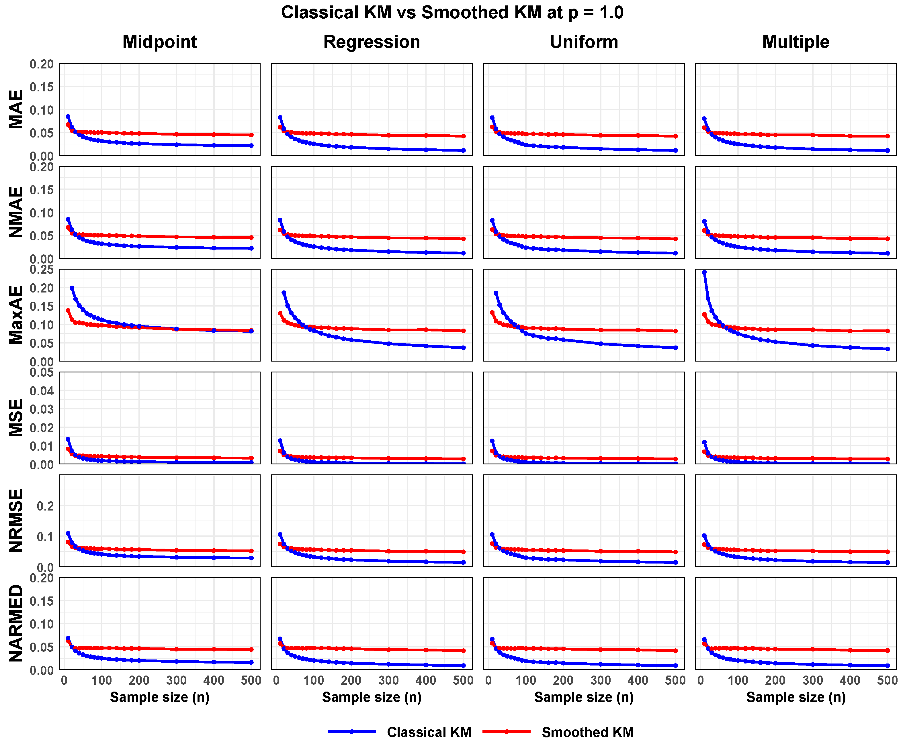
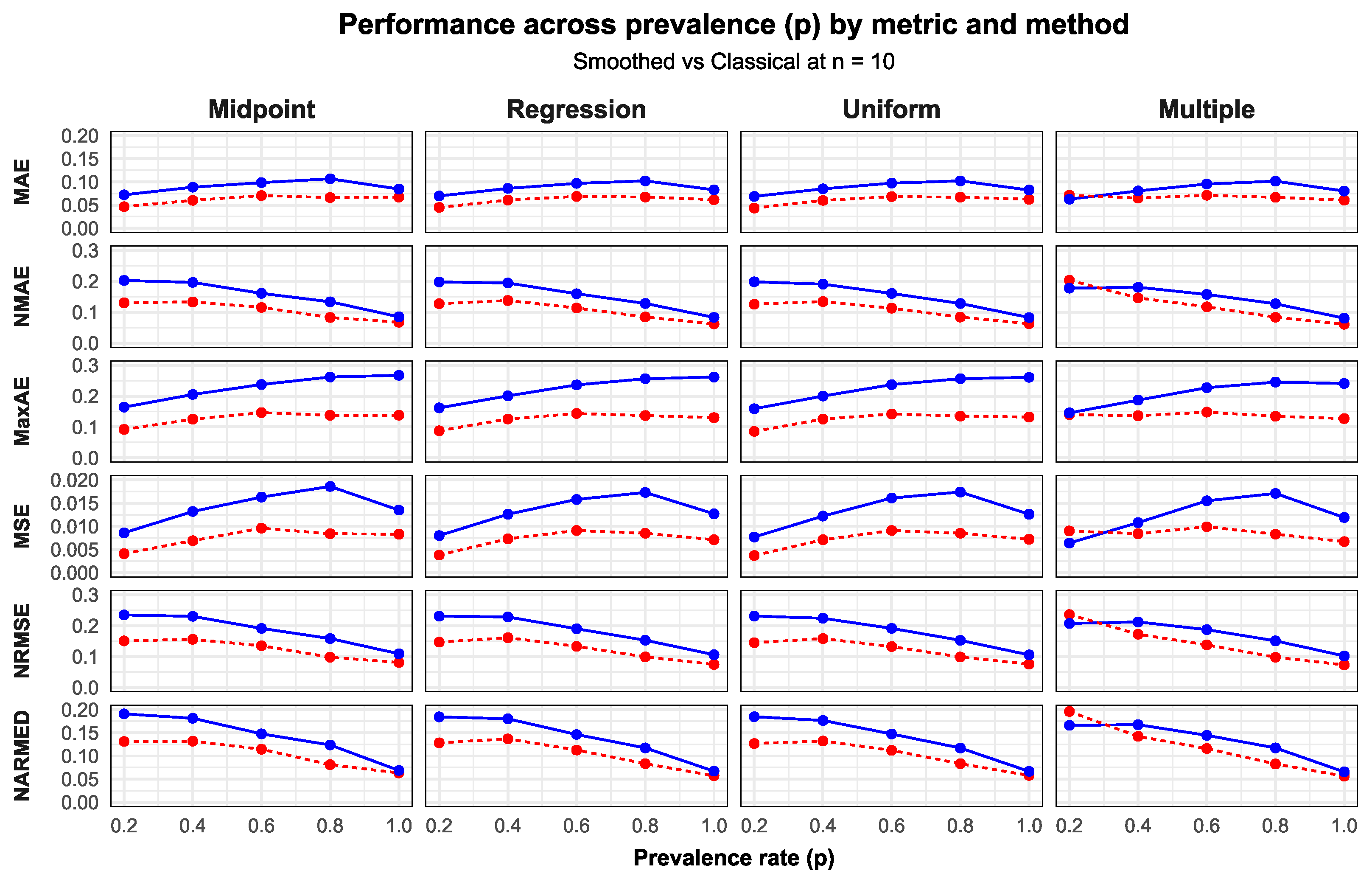
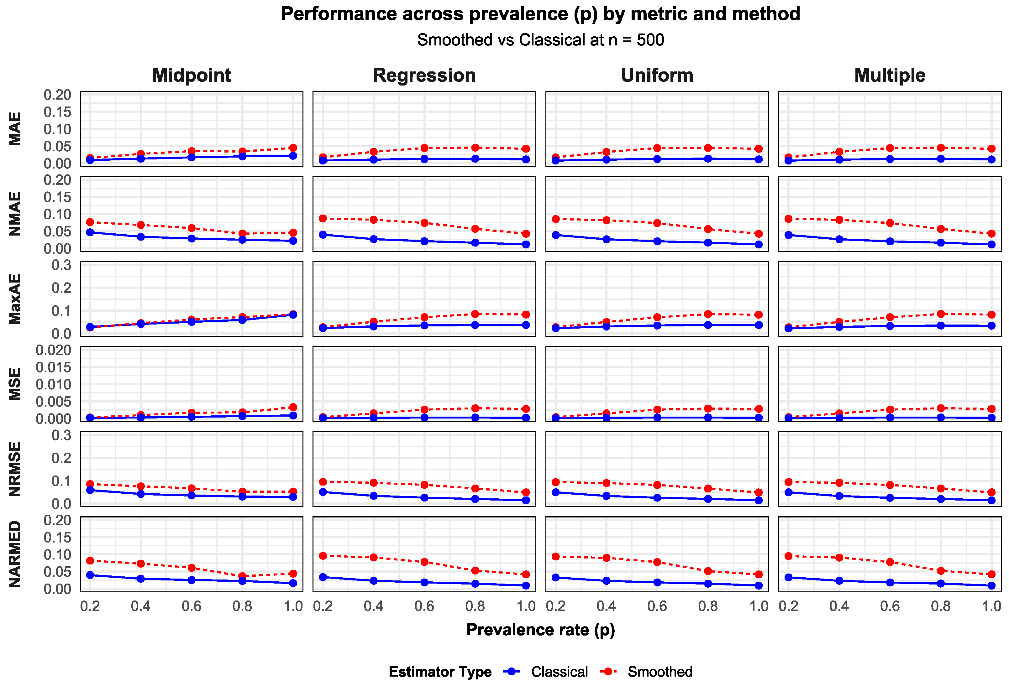
3.2.2. Monte Carlo Performance Evaluation of the KM-Based Estimators
3.2.3. Convergence Validation for Simulated Data
3.3. Empirical Study
3.3.1. Real Data Description
3.3.2. Real Data Bootstrapping Procedure
- Randomly sample n observations with a replacement from the ACTG181 dataset;
- Impute event times using the same imputation method under consideration;
- Fit a KM survival curve on ;
- Interpolate the resulting KM step function onto the common time grid.
3.4. Real Data Application Results
3.4.1. Descriptive Analysis for the ACTG181 Data
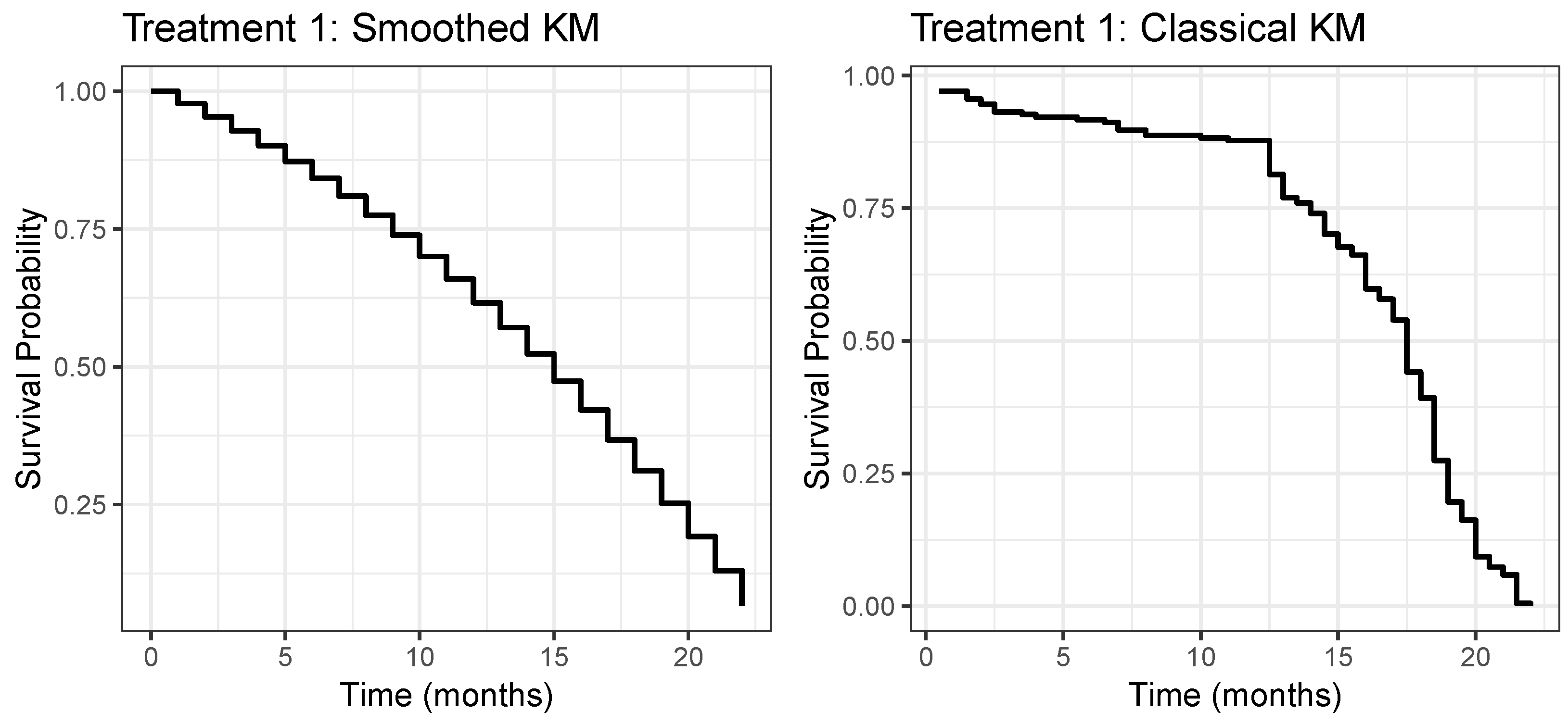
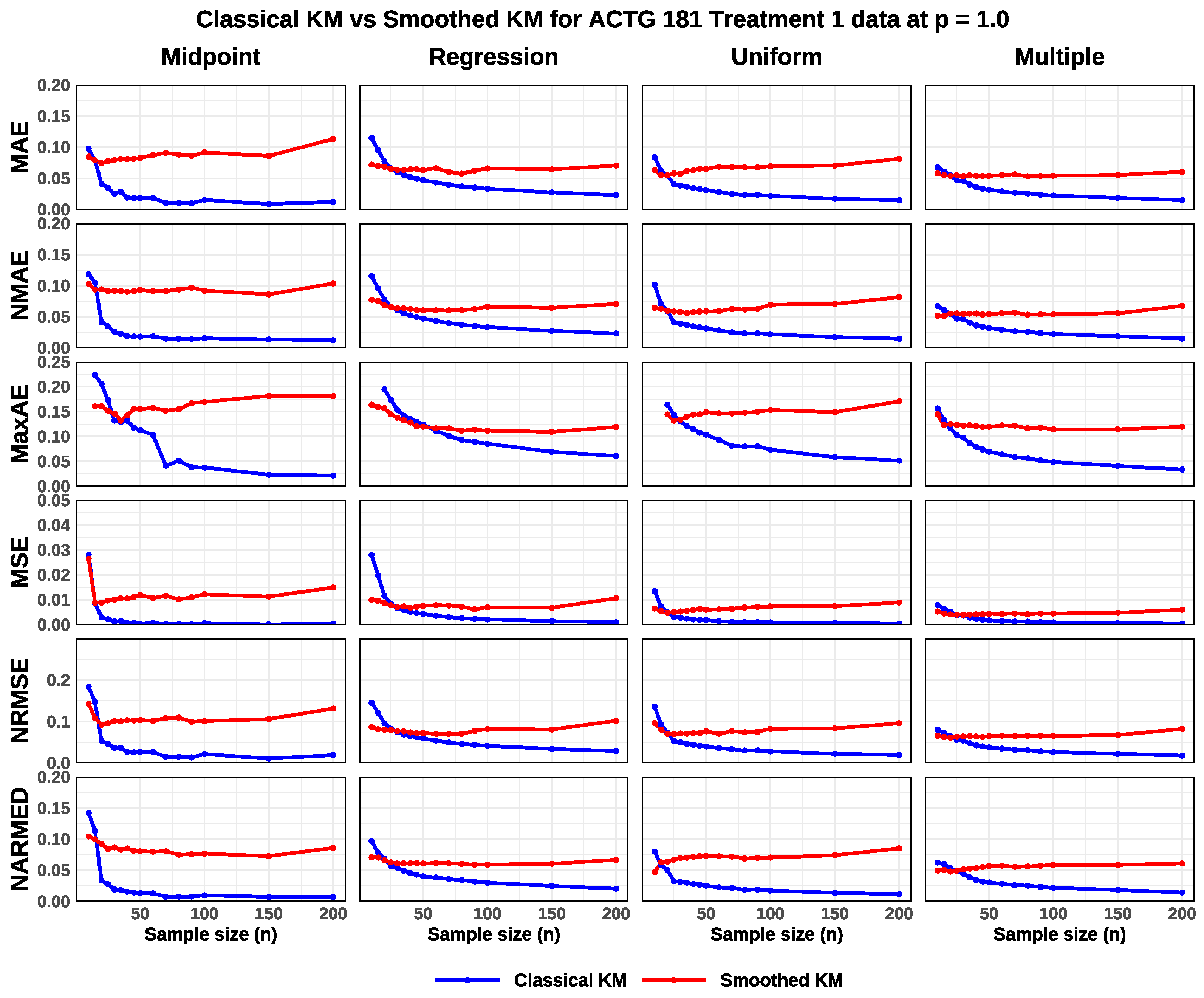
3.4.2. Real Data Bootstrap Resampling Results
3.4.3. Convergence Validation for ACTG181 Real Data
4. Discussion and Conclusions
Author Contributions
Funding
Data Availability Statement
Acknowledgments
Conflicts of Interest
Appendix A

| Symbol/Abbreviation | Description |
|---|---|
| T | True (unobserved) event or failure time |
| L | Left endpoint of the censoring interval |
| R | Right endpoint of the censoring interval |
| I | Interval within which the event time lies |
| n | Sample size |
| p | Prevalence rate |
| Time point i at which survival is evaluated | |
| True survival function at time t | |
| Estimated survival function at time t | |
| Estimated survival probability at time point i | |
| R (normalization) | Range of the true survival function, used for normalization |
| Convergence threshold or error tolerance | |
| KM | Kaplan–Meier |
| TB | Turnbull |
| NPMLE | Nonparametric Maximum Likelihood Estimator |
| MLE | Maximum Likelihood Estimation |
| MI | Multiple Imputation |
| AFT | Accelerated Failure Time |
| MC | Monte Carlo |
| MAE | Mean Absolute Error |
| NMAE | Normalized Mean Absolute Error |
| MaxAE | Maximum Absolute Error |
| MSE | Mean Squared Error |
| NRMSE | Normalized Root Mean Squared Error |
| NARMED | Normalized Root Median Error Deviation |
| MAC | Mycobacterium Avium Complex |
| CMV | Cytomegalovirus |
| HIV | Human Immunodeficiency Virus |
| AIDS | Acquired Immunodeficiency Syndrome |
| ACTG | AIDS Clinical Trials Group |
| Metric | Imputation Methods | ||||||||
|---|---|---|---|---|---|---|---|---|---|
| Midpoint | Regression | Uniform | Multiple | ||||||
| Smoothed | Classical | Smoothed | Classical | Smoothed | Classical | Smoothed | Classical | ||
| 10 | MAE | 0.0465 | 0.0721 | 0.0449 | 0.0696 | 0.0436 | 0.0687 | 0.0713 | 0.0627 |
| NMAE | 0.1305 | 0.2025 | 0.1274 | 0.1976 | 0.1257 | 0.1982 | 0.2032 | 0.1775 | |
| MaxAE | 0.0920 | 0.1641 | 0.0877 | 0.1617 | 0.0855 | 0.1590 | 0.1398 | 0.1455 | |
| MSE | 0.0041 | 0.0086 | 0.0038 | 0.0080 | 0.0037 | 0.0077 | 0.0090 | 0.0064 | |
| NRMSE | 0.1507 | 0.2348 | 0.1467 | 0.2306 | 0.1449 | 0.2310 | 0.2360 | 0.2072 | |
| NARMED | 0.1312 | 0.1907 | 0.1283 | 0.1842 | 0.1267 | 0.1846 | 0.1958 | 0.1660 | |
| 20 | MAE | 0.0328 | 0.0476 | 0.0329 | 0.0458 | 0.0328 | 0.0454 | 0.0360 | 0.0419 |
| NMAE | 0.1402 | 0.2032 | 0.1435 | 0.1997 | 0.1418 | 0.1961 | 0.1564 | 0.1821 | |
| MaxAE | 0.0707 | 0.1116 | 0.0702 | 0.1094 | 0.0700 | 0.1083 | 0.0777 | 0.0988 | |
| MSE | 0.0022 | 0.0040 | 0.0022 | 0.0037 | 0.0022 | 0.0036 | 0.0027 | 0.0030 | |
| NRMSE | 0.1660 | 0.2395 | 0.1701 | 0.2364 | 0.1681 | 0.2318 | 0.1859 | 0.2149 | |
| NARMED | 0.1361 | 0.1862 | 0.1408 | 0.1831 | 0.1377 | 0.1786 | 0.1497 | 0.1672 | |
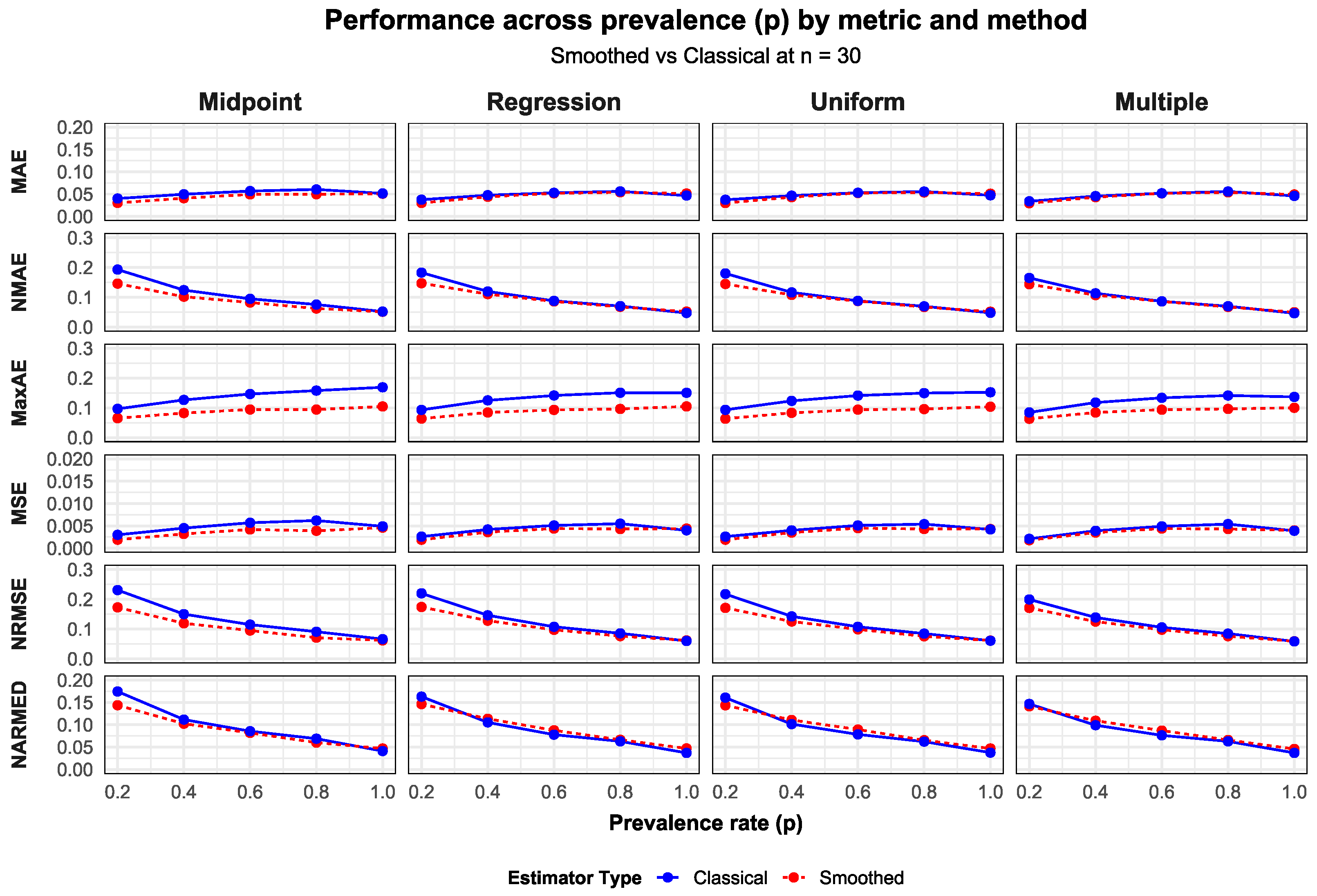
| 30 | MAE | 0.0303 | 0.0401 | 0.0302 | 0.0375 | 0.0300 | 0.0373 | 0.0295 | 0.0339 |
| NMAE | 0.1458 | 0.1930 | 0.1471 | 0.1828 | 0.1445 | 0.1800 | 0.1437 | 0.1650 | |
| MaxAE | 0.0653 | 0.0967 | 0.0639 | 0.0932 | 0.0635 | 0.0933 | 0.0633 | 0.0847 | |
| MSE | 0.0019 | 0.0030 | 0.0019 | 0.0026 | 0.0019 | 0.0026 | 0.0018 | 0.0021 | |
| NRMSE | 0.1727 | 0.2309 | 0.1741 | 0.2201 | 0.1710 | 0.2173 | 0.1709 | 0.1995 | |
| NARMED | 0.1437 | 0.1745 | 0.1462 | 0.1630 | 0.1435 | 0.1607 | 0.1413 | 0.1466 | |
| 40 | MAE | 0.0266 | 0.0338 | 0.0271 | 0.0311 | 0.0270 | 0.0314 | 0.0275 | 0.0296 |
| NMAE | 0.1319 | 0.1678 | 0.1336 | 0.1532 | 0.1344 | 0.1562 | 0.1379 | 0.1483 | |
| MaxAE | 0.0574 | 0.0849 | 0.0569 | 0.0812 | 0.0563 | 0.0815 | 0.0573 | 0.0755 | |
| MSE | 0.0015 | 0.0021 | 0.0015 | 0.0018 | 0.0015 | 0.0019 | 0.0015 | 0.0017 | |
| NRMSE | 0.1568 | 0.2036 | 0.1582 | 0.1867 | 0.1590 | 0.1905 | 0.1629 | 0.1807 | |
| NARMED | 0.1299 | 0.1483 | 0.1330 | 0.1342 | 0.1339 | 0.1358 | 0.1385 | 0.1298 | |
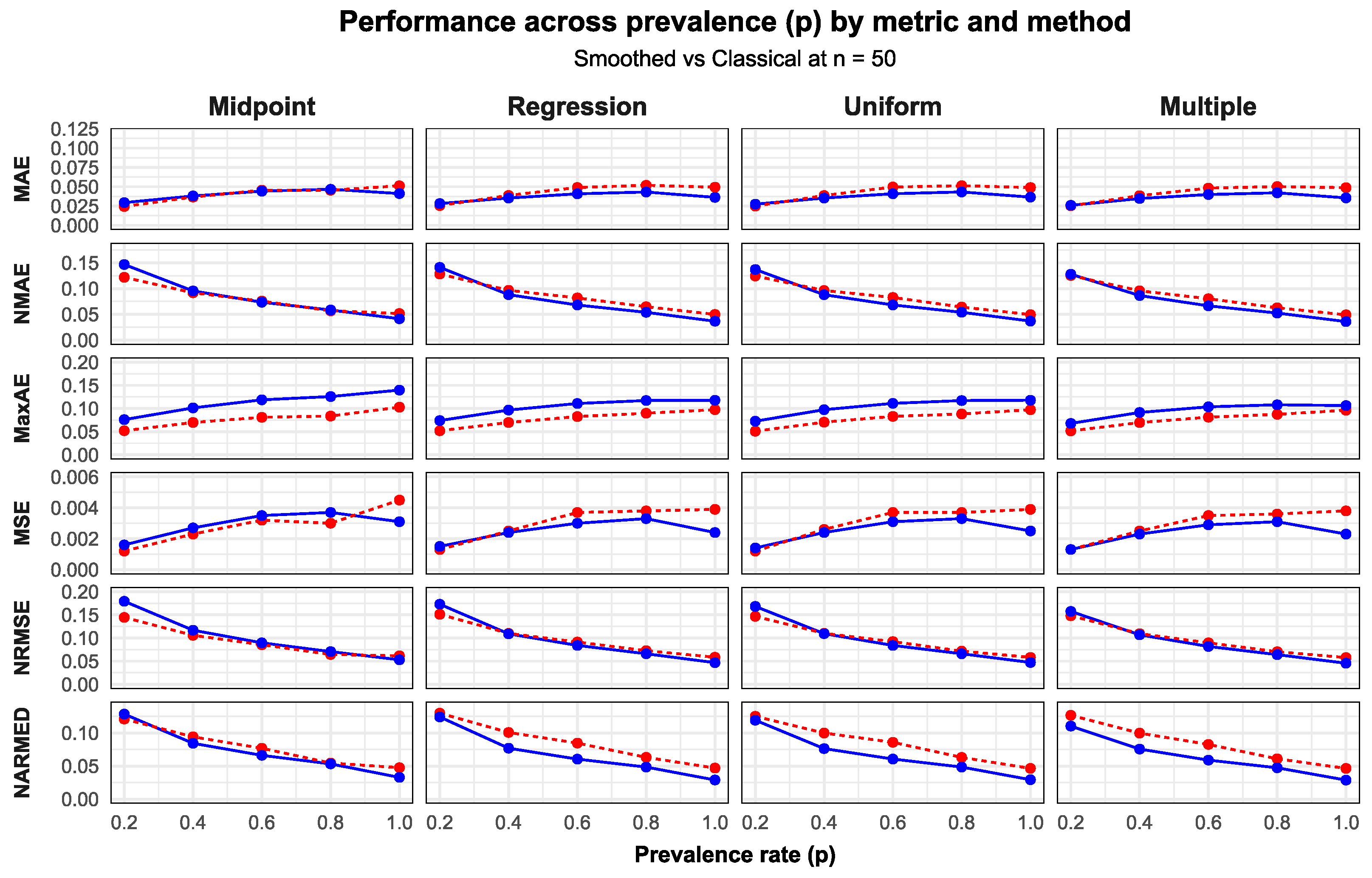
| 50 | MAE | 0.0244 | 0.0294 | 0.0256 | 0.0282 | 0.0249 | 0.0274 | 0.0253 | 0.0259 |
| NMAE | 0.1219 | 0.1468 | 0.1284 | 0.1413 | 0.1245 | 0.1371 | 0.1254 | 0.1279 | |
| MaxAE | 0.0520 | 0.0760 | 0.0520 | 0.0740 | 0.0510 | 0.0726 | 0.0517 | 0.0678 | |
| MSE | 0.0012 | 0.0016 | 0.0013 | 0.0015 | 0.0012 | 0.0014 | 0.0013 | 0.0013 | |
| NRMSE | 0.1445 | 0.1793 | 0.1512 | 0.1729 | 0.1467 | 0.1682 | 0.1481 | 0.1574 | |
| NARMED | 0.1210 | 0.1284 | 0.1298 | 0.1241 | 0.1251 | 0.1192 | 0.1266 | 0.1103 | |
| 80 | MAE | 0.0213 | 0.0228 | 0.0219 | 0.0210 | 0.0224 | 0.0213 | 0.0214 | 0.0200 |
| NMAE | 0.1066 | 0.1142 | 0.1103 | 0.1058 | 0.1117 | 0.1061 | 0.1061 | 0.0994 | |
| MaxAE | 0.0431 | 0.0607 | 0.0421 | 0.0575 | 0.0435 | 0.0585 | 0.0419 | 0.0540 | |
| MSE | 0.0009 | 0.0010 | 0.0009 | 0.0009 | 0.0009 | 0.0009 | 0.0009 | 0.0008 | |
| NRMSE | 0.1248 | 0.1407 | 0.1284 | 0.1315 | 0.1302 | 0.1319 | 0.1240 | 0.1239 | |
| NARMED | 0.1083 | 0.1003 | 0.1134 | 0.0908 | 0.1147 | 0.0915 | 0.1085 | 0.0848 | |
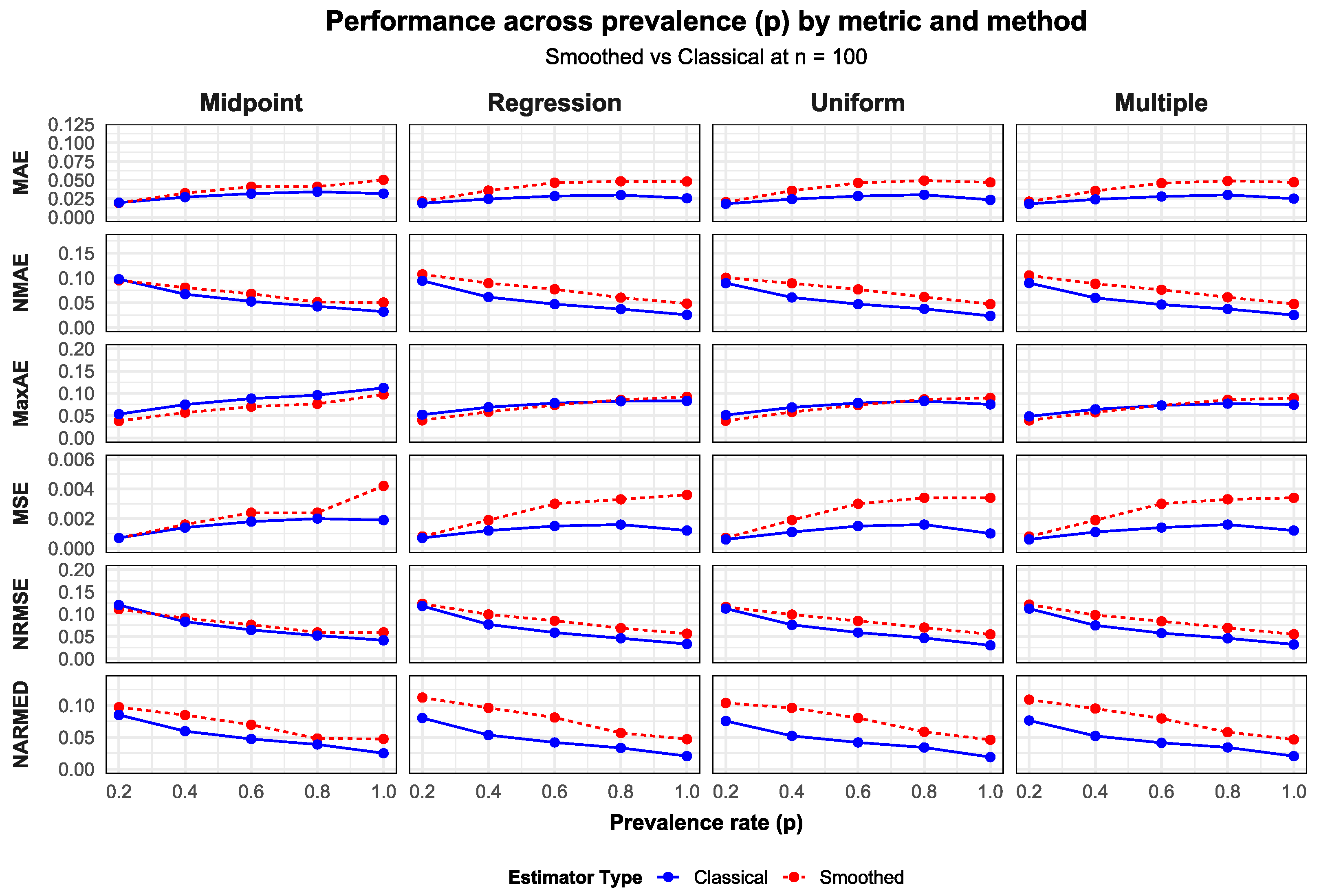
| 100 | MAE | 0.0191 | 0.0196 | 0.0213 | 0.0188 | 0.0202 | 0.0180 | 0.0210 | 0.0179 |
| NMAE | 0.0953 | 0.0976 | 0.1074 | 0.0944 | 0.1005 | 0.0898 | 0.1052 | 0.0899 | |
| MaxAE | 0.0382 | 0.0535 | 0.0396 | 0.0523 | 0.0385 | 0.0513 | 0.0394 | 0.0485 | |
| MSE | 0.0007 | 0.0007 | 0.0008 | 0.0007 | 0.0007 | 0.0006 | 0.0008 | 0.0006 | |
| NRMSE | 0.1112 | 0.1204 | 0.1233 | 0.1182 | 0.1163 | 0.1126 | 0.1214 | 0.1124 | |
| NARMED | 0.0972 | 0.0851 | 0.1124 | 0.0803 | 0.1039 | 0.0756 | 0.1091 | 0.0764 | |
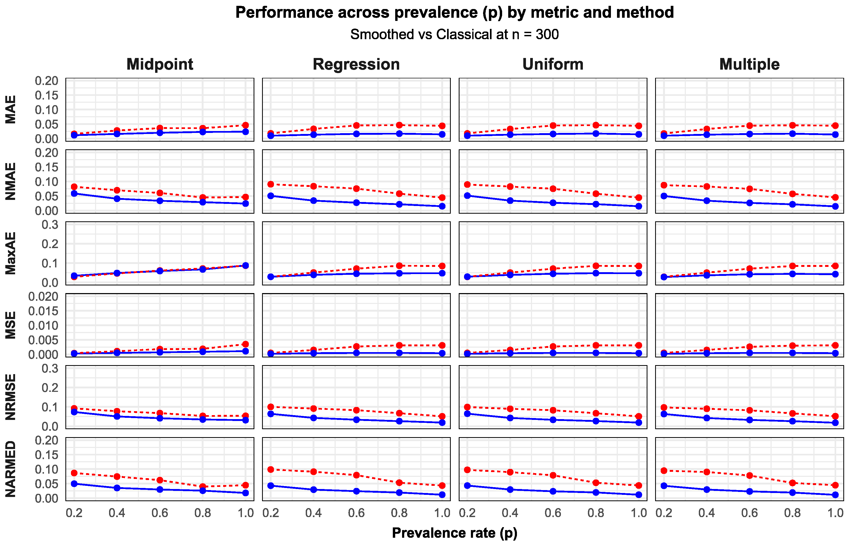
| 300 | MAE | 0.0163 | 0.0117 | 0.0180 | 0.0101 | 0.0179 | 0.0102 | 0.0176 | 0.0101 |
| NMAE | 0.0818 | 0.0587 | 0.0905 | 0.0506 | 0.0896 | 0.0513 | 0.0874 | 0.0501 | |
| MaxAE | 0.0290 | 0.0345 | 0.0292 | 0.0294 | 0.0292 | 0.0298 | 0.0291 | 0.0280 | |
| MSE | 0.0004 | 0.0003 | 0.0005 | 0.0002 | 0.0005 | 0.0002 | 0.0005 | 0.0002 | |
| NRMSE | 0.0922 | 0.0738 | 0.1000 | 0.0641 | 0.0993 | 0.0651 | 0.0971 | 0.0634 | |
| NARMED | 0.0867 | 0.0498 | 0.0988 | 0.0431 | 0.0975 | 0.0434 | 0.0947 | 0.0427 | |
| 500 | MAE | 0.0153 | 0.0094 | 0.0174 | 0.0080 | 0.0171 | 0.0078 | 0.0172 | 0.0078 |
| NMAE | 0.0762 | 0.0467 | 0.0871 | 0.0399 | 0.0854 | 0.0388 | 0.0859 | 0.0388 | |
| MaxAE | 0.0260 | 0.0285 | 0.0273 | 0.0233 | 0.0273 | 0.0229 | 0.0269 | 0.0217 | |
| MSE | 0.0003 | 0.0002 | 0.0004 | 0.0001 | 0.0004 | 0.0001 | 0.0004 | 0.0001 | |
| NRMSE | 0.0851 | 0.0590 | 0.0955 | 0.0507 | 0.0939 | 0.0494 | 0.0943 | 0.0493 | |
| NARMED | 0.0817 | 0.0396 | 0.0958 | 0.0338 | 0.0934 | 0.0326 | 0.0948 | 0.0331 | |
| Metric | Imputation Methods | ||||||||
|---|---|---|---|---|---|---|---|---|---|
| Midpoint | Regression | Uniform | Multiple | ||||||
| Smoothed | Classical | Smoothed | Classical | Smoothed | Classical | Smoothed | Classical | ||
| 10 | MAE | 0.0601 | 0.0886 | 0.0608 | 0.0859 | 0.0600 | 0.0850 | 0.0651 | 0.0805 |
| NMAE | 0.1332 | 0.1963 | 0.1377 | 0.1944 | 0.1344 | 0.1905 | 0.1461 | 0.1805 | |
| MaxAE | 0.1252 | 0.2051 | 0.1258 | 0.2006 | 0.1255 | 0.1999 | 0.1363 | 0.1868 | |
| MSE | 0.0069 | 0.0132 | 0.0073 | 0.0126 | 0.0071 | 0.0122 | 0.0084 | 0.0108 | |
| NRMSE | 0.1558 | 0.2301 | 0.1611 | 0.2282 | 0.1582 | 0.2239 | 0.1722 | 0.2121 | |
| NARMED | 0.1318 | 0.1812 | 0.1368 | 0.1801 | 0.1321 | 0.1765 | 0.1422 | 0.1674 | |
| 20 | MAE | 0.0470 | 0.0620 | 0.0497 | 0.0602 | 0.0495 | 0.0597 | 0.0470 | 0.0561 |
| NMAE | 0.1174 | 0.1549 | 0.1229 | 0.1489 | 0.1234 | 0.1488 | 0.1164 | 0.1391 | |
| MaxAE | 0.0996 | 0.1542 | 0.1006 | 0.1523 | 0.1013 | 0.1521 | 0.0965 | 0.1407 | |
| MSE | 0.0043 | 0.0068 | 0.0048 | 0.0066 | 0.0048 | 0.0065 | 0.0044 | 0.0057 | |
| NRMSE | 0.1385 | 0.1862 | 0.1443 | 0.1801 | 0.1450 | 0.1800 | 0.1373 | 0.1683 | |
| NARMED | 0.1167 | 0.1397 | 0.1235 | 0.1331 | 0.1241 | 0.1321 | 0.1157 | 0.1235 | |
| 30 | MAE | 0.0408 | 0.0496 | 0.0440 | 0.0475 | 0.0431 | 0.0465 | 0.0431 | 0.0455 |
| NMAE | 0.1018 | 0.1240 | 0.1104 | 0.1194 | 0.1079 | 0.1163 | 0.1072 | 0.1132 | |
| MaxAE | 0.0825 | 0.1266 | 0.0844 | 0.1251 | 0.0832 | 0.1234 | 0.0843 | 0.1178 | |
| MSE | 0.0032 | 0.0045 | 0.0036 | 0.0042 | 0.0035 | 0.0040 | 0.0035 | 0.0039 | |
| NRMSE | 0.1194 | 0.1501 | 0.1281 | 0.1462 | 0.1253 | 0.1426 | 0.1251 | 0.1389 | |
| NARMED | 0.1024 | 0.1116 | 0.1134 | 0.1053 | 0.1107 | 0.1015 | 0.1090 | 0.0990 | |
| 40 | MAE | 0.0384 | 0.0426 | 0.0401 | 0.0398 | 0.0406 | 0.0399 | 0.0399 | 0.0391 |
| NMAE | 0.0960 | 0.1065 | 0.0999 | 0.0992 | 0.1017 | 0.1000 | 0.0998 | 0.0978 | |
| MaxAE | 0.0746 | 0.1110 | 0.0752 | 0.1076 | 0.0753 | 0.1079 | 0.0745 | 0.1017 | |
| MSE | 0.0027 | 0.0034 | 0.0029 | 0.0030 | 0.0029 | 0.0030 | 0.0028 | 0.0029 | |
| NRMSE | 0.1113 | 0.1299 | 0.1152 | 0.1223 | 0.1168 | 0.1233 | 0.1149 | 0.1202 | |
| NARMED | 0.0981 | 0.0948 | 0.1029 | 0.0863 | 0.1054 | 0.0872 | 0.1028 | 0.0853 | |
| 50 | MAE | 0.0366 | 0.0380 | 0.0387 | 0.0353 | 0.0386 | 0.0353 | 0.0384 | 0.0347 |
| NMAE | 0.0918 | 0.0954 | 0.0966 | 0.0882 | 0.0963 | 0.0881 | 0.0957 | 0.0865 | |
| MaxAE | 0.0698 | 0.1013 | 0.0698 | 0.0966 | 0.0705 | 0.0974 | 0.0696 | 0.0914 | |
| MSE | 0.0023 | 0.0027 | 0.0025 | 0.0024 | 0.0026 | 0.0024 | 0.0025 | 0.0023 | |
| NRMSE | 0.1058 | 0.1168 | 0.1100 | 0.1090 | 0.1101 | 0.1094 | 0.1094 | 0.1069 | |
| NARMED | 0.0941 | 0.0843 | 0.1007 | 0.0769 | 0.0998 | 0.0763 | 0.0997 | 0.0756 | |
| 80 | MAE | 0.0333 | 0.0298 | 0.0361 | 0.0276 | 0.0366 | 0.0276 | 0.0363 | 0.0271 |
| NMAE | 0.0832 | 0.0745 | 0.0901 | 0.0688 | 0.0915 | 0.0689 | 0.0908 | 0.0677 | |
| MaxAE | 0.0600 | 0.0820 | 0.0616 | 0.0776 | 0.0620 | 0.0769 | 0.0612 | 0.0721 | |
| MSE | 0.0018 | 0.0017 | 0.0021 | 0.0015 | 0.0021 | 0.0015 | 0.0021 | 0.0014 | |
| NRMSE | 0.0943 | 0.0920 | 0.1011 | 0.0861 | 0.1025 | 0.0858 | 0.1016 | 0.0844 | |
| NARMED | 0.0871 | 0.0658 | 0.0957 | 0.0593 | 0.0979 | 0.0599 | 0.0968 | 0.0589 | |
| 100 | MAE | 0.0323 | 0.0270 | 0.0358 | 0.0245 | 0.0356 | 0.0243 | 0.0353 | 0.0240 |
| NMAE | 0.0807 | 0.0674 | 0.0897 | 0.0615 | 0.0893 | 0.0608 | 0.0883 | 0.0599 | |
| MaxAE | 0.0570 | 0.0749 | 0.0588 | 0.0690 | 0.0583 | 0.0686 | 0.0577 | 0.0642 | |
| MSE | 0.0016 | 0.0014 | 0.0019 | 0.0012 | 0.0019 | 0.0011 | 0.0019 | 0.0011 | |
| NRMSE | 0.0909 | 0.0832 | 0.0995 | 0.0770 | 0.0991 | 0.0761 | 0.0980 | 0.0748 | |
| NARMED | 0.0849 | 0.0596 | 0.0962 | 0.0535 | 0.0962 | 0.0522 | 0.0951 | 0.0521 | |
| 300 | MAE | 0.0279 | 0.0162 | 0.0334 | 0.0136 | 0.0330 | 0.0137 | 0.0331 | 0.0136 |
| NMAE | 0.0698 | 0.0406 | 0.0836 | 0.0341 | 0.0824 | 0.0341 | 0.0827 | 0.0339 | |
| MaxAE | 0.0466 | 0.0486 | 0.0511 | 0.0393 | 0.0508 | 0.0390 | 0.0506 | 0.0367 | |
| MSE | 0.0011 | 0.0005 | 0.0015 | 0.0004 | 0.0015 | 0.0004 | 0.0015 | 0.0004 | |
| NRMSE | 0.0777 | 0.0507 | 0.0915 | 0.0432 | 0.0901 | 0.0429 | 0.0904 | 0.0426 | |
| NARMED | 0.0744 | 0.0352 | 0.0911 | 0.0294 | 0.0897 | 0.0297 | 0.0902 | 0.0297 | |
| 500 | MAE | 0.0273 | 0.0135 | 0.0334 | 0.0107 | 0.0328 | 0.0106 | 0.0333 | 0.0106 |
| NMAE | 0.0680 | 0.0337 | 0.0833 | 0.0268 | 0.0821 | 0.0264 | 0.0831 | 0.0264 | |
| MaxAE | 0.0449 | 0.0413 | 0.0509 | 0.0308 | 0.0501 | 0.0303 | 0.0505 | 0.0286 | |
| MSE | 0.0010 | 0.0003 | 0.0015 | 0.0002 | 0.0014 | 0.0002 | 0.0015 | 0.0002 | |
| NRMSE | 0.0757 | 0.0421 | 0.0910 | 0.0339 | 0.0898 | 0.0334 | 0.0908 | 0.0332 | |
| NARMED | 0.0728 | 0.0291 | 0.0909 | 0.0231 | 0.0897 | 0.0229 | 0.0905 | 0.0230 | |
| Metric | Imputation Methods | ||||||||
|---|---|---|---|---|---|---|---|---|---|
| Midpoint | Regression | Uniform | Multiple | ||||||
| Smoothed | Classical | Smoothed | Classical | Smoothed | Classical | Smoothed | Classical | ||
| 10 | MAE | 0.0705 | 0.0984 | 0.0688 | 0.0968 | 0.0683 | 0.0973 | 0.0711 | 0.0954 |
| NMAE | 0.1152 | 0.1608 | 0.1134 | 0.1596 | 0.1128 | 0.1605 | 0.1173 | 0.1574 | |
| MaxAE | 0.1463 | 0.2374 | 0.1434 | 0.2360 | 0.1418 | 0.2369 | 0.1480 | 0.2270 | |
| MSE | 0.0096 | 0.0163 | 0.0091 | 0.0158 | 0.0091 | 0.0161 | 0.0099 | 0.0155 | |
| NRMSE | 0.1350 | 0.1912 | 0.1332 | 0.1899 | 0.1323 | 0.1912 | 0.1379 | 0.1871 | |
| NARMED | 0.1144 | 0.1476 | 0.1127 | 0.1462 | 0.1120 | 0.1473 | 0.1159 | 0.1444 | |
| 20 | MAE | 0.0547 | 0.0707 | 0.0571 | 0.0670 | 0.0583 | 0.0678 | 0.0559 | 0.0656 |
| NMAE | 0.0911 | 0.1178 | 0.0954 | 0.1118 | 0.0971 | 0.1129 | 0.0933 | 0.1102 | |
| MaxAE | 0.1094 | 0.1779 | 0.1090 | 0.1732 | 0.1108 | 0.1751 | 0.1082 | 0.1642 | |
| MSE | 0.0055 | 0.0087 | 0.0058 | 0.0079 | 0.0060 | 0.0082 | 0.0056 | 0.0077 | |
| NRMSE | 0.1063 | 0.1415 | 0.1099 | 0.1355 | 0.1119 | 0.1368 | 0.1080 | 0.1334 | |
| NARMED | 0.0905 | 0.1070 | 0.0968 | 0.0999 | 0.0985 | 0.1011 | 0.0933 | 0.0989 | |
| 30 | MAE | 0.0493 | 0.0568 | 0.0517 | 0.0529 | 0.0524 | 0.0530 | 0.0516 | 0.0519 |
| NMAE | 0.0823 | 0.0947 | 0.0859 | 0.0879 | 0.0871 | 0.0880 | 0.0858 | 0.0863 | |
| MaxAE | 0.0944 | 0.1464 | 0.0931 | 0.1415 | 0.0940 | 0.1413 | 0.0937 | 0.1336 | |
| MSE | 0.0042 | 0.0057 | 0.0044 | 0.0051 | 0.0045 | 0.0051 | 0.0044 | 0.0049 | |
| NRMSE | 0.0950 | 0.1149 | 0.0975 | 0.1076 | 0.0989 | 0.1076 | 0.0977 | 0.1056 | |
| NARMED | 0.0818 | 0.0856 | 0.0875 | 0.0778 | 0.0893 | 0.0784 | 0.0870 | 0.0763 | |
| 40 | MAE | 0.0458 | 0.0486 | 0.0511 | 0.0458 | 0.0502 | 0.0455 | 0.0498 | 0.0448 |
| NMAE | 0.0762 | 0.0808 | 0.0852 | 0.0764 | 0.0837 | 0.0758 | 0.0829 | 0.0747 | |
| MaxAE | 0.0845 | 0.1289 | 0.0875 | 0.1241 | 0.0866 | 0.1230 | 0.0860 | 0.1158 | |
| MSE | 0.0034 | 0.0042 | 0.0041 | 0.0038 | 0.0040 | 0.0038 | 0.0039 | 0.0037 | |
| NRMSE | 0.0867 | 0.0983 | 0.0955 | 0.0940 | 0.0939 | 0.0933 | 0.0930 | 0.0916 | |
| NARMED | 0.0769 | 0.0727 | 0.0884 | 0.0673 | 0.0867 | 0.0672 | 0.0849 | 0.0661 | |
| 50 | MAE | 0.0455 | 0.0442 | 0.0490 | 0.0408 | 0.0496 | 0.0409 | 0.0482 | 0.0399 |
| NMAE | 0.0757 | 0.0735 | 0.0819 | 0.0681 | 0.0828 | 0.0682 | 0.0803 | 0.0665 | |
| MaxAE | 0.0810 | 0.1187 | 0.0826 | 0.1108 | 0.0830 | 0.1111 | 0.0813 | 0.1036 | |
| MSE | 0.0032 | 0.0035 | 0.0037 | 0.0030 | 0.0037 | 0.0031 | 0.0035 | 0.0029 | |
| NRMSE | 0.0855 | 0.0896 | 0.0913 | 0.0840 | 0.0922 | 0.0840 | 0.0896 | 0.0818 | |
| NARMED | 0.0768 | 0.0661 | 0.0846 | 0.0604 | 0.0858 | 0.0605 | 0.0826 | 0.0589 | |
| 80 | MAE | 0.0420 | 0.0349 | 0.0461 | 0.0315 | 0.0468 | 0.0314 | 0.0469 | 0.0313 |
| NMAE | 0.0699 | 0.0580 | 0.0767 | 0.0524 | 0.0779 | 0.0523 | 0.0782 | 0.0522 | |
| MaxAE | 0.0725 | 0.0964 | 0.0749 | 0.0872 | 0.0760 | 0.0869 | 0.0754 | 0.0816 | |
| MSE | 0.0026 | 0.0022 | 0.0031 | 0.0018 | 0.0031 | 0.0018 | 0.0031 | 0.0018 | |
| NRMSE | 0.0783 | 0.0711 | 0.0848 | 0.0650 | 0.0862 | 0.0648 | 0.0863 | 0.0644 | |
| NARMED | 0.0716 | 0.0519 | 0.0796 | 0.0461 | 0.0811 | 0.0461 | 0.0816 | 0.0466 | |
| 100 | MAE | 0.0410 | 0.0317 | 0.0464 | 0.0284 | 0.0461 | 0.0284 | 0.0458 | 0.0278 |
| NMAE | 0.0682 | 0.0527 | 0.0774 | 0.0472 | 0.0770 | 0.0473 | 0.0763 | 0.0464 | |
| MaxAE | 0.0701 | 0.0883 | 0.0737 | 0.0783 | 0.0736 | 0.0785 | 0.0731 | 0.0731 | |
| MSE | 0.0024 | 0.0018 | 0.0030 | 0.0015 | 0.0030 | 0.0015 | 0.0030 | 0.0014 | |
| NRMSE | 0.0762 | 0.0646 | 0.0852 | 0.0586 | 0.0848 | 0.0588 | 0.0841 | 0.0575 | |
| NARMED | 0.0697 | 0.0473 | 0.0811 | 0.0419 | 0.0803 | 0.0419 | 0.0796 | 0.0413 | |
| 300 | MAE | 0.0363 | 0.0201 | 0.0453 | 0.0163 | 0.0451 | 0.0160 | 0.0447 | 0.0158 |
| NMAE | 0.0605 | 0.0336 | 0.0754 | 0.0271 | 0.0750 | 0.0267 | 0.0746 | 0.0263 | |
| MaxAE | 0.0614 | 0.0589 | 0.0712 | 0.0451 | 0.0711 | 0.0448 | 0.0712 | 0.0421 | |
| MSE | 0.0018 | 0.0007 | 0.0027 | 0.0005 | 0.0027 | 0.0005 | 0.0026 | 0.0005 | |
| NRMSE | 0.0680 | 0.0414 | 0.0831 | 0.0338 | 0.0827 | 0.0333 | 0.0824 | 0.0328 | |
| NARMED | 0.0621 | 0.0299 | 0.0793 | 0.0241 | 0.0788 | 0.0236 | 0.0780 | 0.0233 | |
| 500 | MAE | 0.0352 | 0.0171 | 0.0444 | 0.0125 | 0.0443 | 0.0124 | 0.0442 | 0.0122 |
| NMAE | 0.0589 | 0.0287 | 0.0740 | 0.0209 | 0.0737 | 0.0206 | 0.0736 | 0.0203 | |
| MaxAE | 0.0608 | 0.0507 | 0.0709 | 0.0350 | 0.0707 | 0.0347 | 0.0706 | 0.0324 | |
| MSE | 0.0017 | 0.0005 | 0.0026 | 0.0003 | 0.0026 | 0.0003 | 0.0026 | 0.0003 | |
| NRMSE | 0.0669 | 0.0354 | 0.0819 | 0.0261 | 0.0816 | 0.0257 | 0.0815 | 0.0253 | |
| NARMED | 0.0609 | 0.0254 | 0.0778 | 0.0185 | 0.0775 | 0.0183 | 0.0777 | 0.0181 | |
| Metric | Imputation Methods | ||||||||
|---|---|---|---|---|---|---|---|---|---|
| Midpoint | Regression | Uniform | Multiple | ||||||
| Smoothed | Classical | Smoothed | Classical | Smoothed | Classical | Smoothed | Classical | ||
| 10 | MAE | 0.0662 | 0.1067 | 0.0673 | 0.1022 | 0.0671 | 0.1022 | 0.0667 | 0.1016 |
| NMAE | 0.0828 | 0.1335 | 0.0844 | 0.1281 | 0.0840 | 0.1280 | 0.0836 | 0.1272 | |
| MaxAE | 0.1378 | 0.2616 | 0.1369 | 0.2561 | 0.1353 | 0.2562 | 0.1346 | 0.2451 | |
| MSE | 0.0084 | 0.0186 | 0.0085 | 0.0173 | 0.0085 | 0.0174 | 0.0083 | 0.0171 | |
| NRMSE | 0.0979 | 0.1583 | 0.0989 | 0.1528 | 0.0986 | 0.1526 | 0.0979 | 0.1509 | |
| NARMED | 0.0811 | 0.1236 | 0.0833 | 0.1173 | 0.0832 | 0.1171 | 0.0827 | 0.1173 | |
| 20 | MAE | 0.0531 | 0.0738 | 0.0573 | 0.0702 | 0.0562 | 0.0693 | 0.0567 | 0.0697 |
| NMAE | 0.0663 | 0.0921 | 0.0716 | 0.0876 | 0.0700 | 0.0865 | 0.0710 | 0.0872 | |
| MaxAE | 0.1054 | 0.1897 | 0.1078 | 0.1841 | 0.1058 | 0.1829 | 0.1063 | 0.1741 | |
| MSE | 0.0047 | 0.0092 | 0.0053 | 0.0085 | 0.0051 | 0.0083 | 0.0052 | 0.0084 | |
| NRMSE | 0.0769 | 0.1105 | 0.0819 | 0.1060 | 0.0802 | 0.1048 | 0.0809 | 0.1050 | |
| NARMED | 0.0641 | 0.0837 | 0.0700 | 0.0791 | 0.0684 | 0.0777 | 0.0699 | 0.0793 | |
| 30 | MAE | 0.0496 | 0.0604 | 0.0540 | 0.0561 | 0.0537 | 0.0556 | 0.0538 | 0.0558 |
| NMAE | 0.0621 | 0.0755 | 0.0676 | 0.0703 | 0.0671 | 0.0695 | 0.0674 | 0.0698 | |
| MaxAE | 0.0943 | 0.1580 | 0.0964 | 0.1508 | 0.0958 | 0.1496 | 0.0964 | 0.1414 | |
| MSE | 0.0039 | 0.0062 | 0.0043 | 0.0055 | 0.0043 | 0.0054 | 0.0043 | 0.0054 | |
| NRMSE | 0.0710 | 0.0910 | 0.0761 | 0.0856 | 0.0756 | 0.0847 | 0.0759 | 0.0846 | |
| NARMED | 0.0600 | 0.0688 | 0.0663 | 0.0629 | 0.0654 | 0.0622 | 0.0659 | 0.0628 | |
| 40 | MAE | 0.0474 | 0.0523 | 0.0524 | 0.0482 | 0.0524 | 0.0485 | 0.0522 | 0.0477 |
| NMAE | 0.0591 | 0.0652 | 0.0653 | 0.0601 | 0.0654 | 0.0605 | 0.0652 | 0.0596 | |
| MaxAE | 0.0875 | 0.1398 | 0.0920 | 0.1301 | 0.0916 | 0.1310 | 0.0915 | 0.1225 | |
| MSE | 0.0034 | 0.0047 | 0.0040 | 0.0041 | 0.0040 | 0.0041 | 0.0039 | 0.0040 | |
| NRMSE | 0.0672 | 0.0788 | 0.0734 | 0.0734 | 0.0734 | 0.0740 | 0.0731 | 0.0726 | |
| NARMED | 0.0572 | 0.0593 | 0.0636 | 0.0538 | 0.0639 | 0.0542 | 0.0638 | 0.0535 | |
| 50 | MAE | 0.0454 | 0.0467 | 0.0518 | 0.0431 | 0.0513 | 0.0432 | 0.0502 | 0.0421 |
| NMAE | 0.0568 | 0.0584 | 0.0648 | 0.0539 | 0.0642 | 0.0540 | 0.0627 | 0.0525 | |
| MaxAE | 0.0837 | 0.1258 | 0.0898 | 0.1172 | 0.0882 | 0.1171 | 0.0874 | 0.1080 | |
| MSE | 0.0030 | 0.0037 | 0.0038 | 0.0033 | 0.0037 | 0.0033 | 0.0036 | 0.0031 | |
| NRMSE | 0.0644 | 0.0706 | 0.0726 | 0.0660 | 0.0717 | 0.0660 | 0.0704 | 0.0641 | |
| NARMED | 0.0545 | 0.0532 | 0.0631 | 0.0484 | 0.0630 | 0.0484 | 0.0609 | 0.0473 | |
| 80 | MAE | 0.0424 | 0.0376 | 0.0496 | 0.0337 | 0.0495 | 0.0336 | 0.0488 | 0.0333 |
| NMAE | 0.0529 | 0.0470 | 0.0619 | 0.0420 | 0.0617 | 0.0419 | 0.0611 | 0.0416 | |
| MaxAE | 0.0776 | 0.1047 | 0.0864 | 0.0925 | 0.0869 | 0.0925 | 0.0851 | 0.0859 | |
| MSE | 0.0026 | 0.0024 | 0.0034 | 0.0020 | 0.0034 | 0.0020 | 0.0034 | 0.0020 | |
| NRMSE | 0.0604 | 0.0571 | 0.0698 | 0.0516 | 0.0697 | 0.0516 | 0.0688 | 0.0510 | |
| NARMED | 0.0505 | 0.0426 | 0.0587 | 0.0378 | 0.0589 | 0.0376 | 0.0586 | 0.0375 | |
| 100 | MAE | 0.0411 | 0.0342 | 0.0483 | 0.0298 | 0.0493 | 0.0302 | 0.0488 | 0.0300 |
| NMAE | 0.0514 | 0.0428 | 0.0604 | 0.0373 | 0.0617 | 0.0378 | 0.0611 | 0.0375 | |
| MaxAE | 0.0765 | 0.0961 | 0.0855 | 0.0825 | 0.0865 | 0.0828 | 0.0856 | 0.0771 | |
| MSE | 0.0024 | 0.0020 | 0.0033 | 0.0016 | 0.0034 | 0.0016 | 0.0033 | 0.0016 | |
| NRMSE | 0.0591 | 0.0520 | 0.0686 | 0.0459 | 0.0699 | 0.0466 | 0.0691 | 0.0459 | |
| NARMED | 0.0482 | 0.0387 | 0.0568 | 0.0333 | 0.0585 | 0.0340 | 0.0580 | 0.0341 | |
| 300 | MAE | 0.0359 | 0.0230 | 0.0465 | 0.0171 | 0.0464 | 0.0175 | 0.0459 | 0.0170 |
| NMAE | 0.0449 | 0.0288 | 0.0581 | 0.0214 | 0.0580 | 0.0219 | 0.0574 | 0.0213 | |
| MaxAE | 0.0718 | 0.0673 | 0.0863 | 0.0472 | 0.0858 | 0.0480 | 0.0851 | 0.0441 | |
| MSE | 0.0019 | 0.0009 | 0.0031 | 0.0005 | 0.0031 | 0.0005 | 0.0030 | 0.0005 | |
| NRMSE | 0.0534 | 0.0351 | 0.0674 | 0.0264 | 0.0672 | 0.0269 | 0.0665 | 0.0262 | |
| NARMED | 0.0398 | 0.0259 | 0.0534 | 0.0193 | 0.0532 | 0.0197 | 0.0525 | 0.0193 | |
| 500 | MAE | 0.0343 | 0.0200 | 0.0454 | 0.0131 | 0.0448 | 0.0134 | 0.0452 | 0.0132 |
| NMAE | 0.0429 | 0.0250 | 0.0568 | 0.0164 | 0.0560 | 0.0167 | 0.0565 | 0.0165 | |
| MaxAE | 0.0714 | 0.0588 | 0.0848 | 0.0365 | 0.0843 | 0.0371 | 0.0851 | 0.0343 | |
| MSE | 0.0018 | 0.0007 | 0.0030 | 0.0003 | 0.0029 | 0.0003 | 0.0030 | 0.0003 | |
| NRMSE | 0.0521 | 0.0306 | 0.0662 | 0.0203 | 0.0655 | 0.0207 | 0.0661 | 0.0203 | |
| NARMED | 0.0364 | 0.0225 | 0.0530 | 0.0147 | 0.0512 | 0.0149 | 0.0520 | 0.0150 | |
| Metric | Imputation Methods | ||||||||
|---|---|---|---|---|---|---|---|---|---|
| Midpoint | Regression | Uniform | Multiple | ||||||
| Smoothed | Classical | Smoothed | Classical | Smoothed | Classical | Smoothed | Classical | ||
| 10 | MAE | 0.0671 | 0.0846 | 0.0617 | 0.0829 | 0.0625 | 0.0824 | 0.0606 | 0.0802 |
| NMAE | 0.0673 | 0.0849 | 0.0618 | 0.0831 | 0.0627 | 0.0826 | 0.0607 | 0.0803 | |
| MaxAE | 0.1379 | 0.2671 | 0.1301 | 0.2614 | 0.1320 | 0.2606 | 0.1271 | 0.2407 | |
| MSE | 0.0083 | 0.0135 | 0.0071 | 0.0127 | 0.0072 | 0.0126 | 0.0067 | 0.0119 | |
| NRMSE | 0.0808 | 0.1091 | 0.0746 | 0.1061 | 0.0756 | 0.1056 | 0.0730 | 0.1020 | |
| NARMED | 0.0632 | 0.0687 | 0.0571 | 0.0671 | 0.0578 | 0.0666 | 0.0563 | 0.0656 | |
| 20 | MAE | 0.0543 | 0.0618 | 0.0538 | 0.0578 | 0.0524 | 0.0576 | 0.0521 | 0.0567 |
| NMAE | 0.0547 | 0.0622 | 0.0541 | 0.0581 | 0.0528 | 0.0580 | 0.0525 | 0.0571 | |
| MaxAE | 0.1133 | 0.1987 | 0.1112 | 0.1860 | 0.1090 | 0.1847 | 0.1077 | 0.1701 | |
| MSE | 0.0054 | 0.0071 | 0.0050 | 0.0062 | 0.0048 | 0.0061 | 0.0047 | 0.0059 | |
| NRMSE | 0.0664 | 0.0794 | 0.0650 | 0.0743 | 0.0635 | 0.0740 | 0.0630 | 0.0724 | |
| NARMED | 0.0497 | 0.0496 | 0.0489 | 0.0458 | 0.0476 | 0.0458 | 0.0476 | 0.0459 | |
| 30 | MAE | 0.0509 | 0.0515 | 0.0513 | 0.0467 | 0.0509 | 0.0473 | 0.0492 | 0.0459 |
| NMAE | 0.0513 | 0.0519 | 0.0517 | 0.0471 | 0.0514 | 0.0477 | 0.0497 | 0.0463 | |
| MaxAE | 0.1046 | 0.1690 | 0.1047 | 0.1506 | 0.1038 | 0.1524 | 0.1001 | 0.1368 | |
| MSE | 0.0046 | 0.0049 | 0.0044 | 0.0040 | 0.0043 | 0.0042 | 0.0040 | 0.0039 | |
| NRMSE | 0.0618 | 0.0661 | 0.0617 | 0.0600 | 0.0613 | 0.0609 | 0.0591 | 0.0585 | |
| NARMED | 0.0468 | 0.0411 | 0.0470 | 0.0370 | 0.0468 | 0.0376 | 0.0457 | 0.0370 | |
| 40 | MAE | 0.0512 | 0.0451 | 0.0504 | 0.0402 | 0.0495 | 0.0409 | 0.0494 | 0.0399 |
| NMAE | 0.0516 | 0.0455 | 0.0509 | 0.0406 | 0.0500 | 0.0413 | 0.0499 | 0.0403 | |
| MaxAE | 0.1047 | 0.1512 | 0.1009 | 0.1307 | 0.0992 | 0.1315 | 0.0987 | 0.1189 | |
| MSE | 0.0046 | 0.0038 | 0.0041 | 0.0030 | 0.0040 | 0.0031 | 0.0040 | 0.0030 | |
| NRMSE | 0.0619 | 0.0581 | 0.0602 | 0.0518 | 0.0591 | 0.0526 | 0.0589 | 0.0510 | |
| NARMED | 0.0468 | 0.0360 | 0.0473 | 0.0318 | 0.0465 | 0.0326 | 0.0467 | 0.0323 | |
| 50 | MAE | 0.0512 | 0.0411 | 0.0494 | 0.0362 | 0.0489 | 0.0365 | 0.0487 | 0.0355 |
| NMAE | 0.0516 | 0.0414 | 0.0498 | 0.0366 | 0.0494 | 0.0369 | 0.0491 | 0.0359 | |
| MaxAE | 0.1029 | 0.1397 | 0.0975 | 0.1178 | 0.0974 | 0.1179 | 0.0962 | 0.1063 | |
| MSE | 0.0045 | 0.0031 | 0.0039 | 0.0024 | 0.0039 | 0.0025 | 0.0038 | 0.0023 | |
| NRMSE | 0.0615 | 0.0530 | 0.0585 | 0.0468 | 0.0582 | 0.0472 | 0.0578 | 0.0456 | |
| NARMED | 0.0475 | 0.0328 | 0.0469 | 0.0289 | 0.0464 | 0.0293 | 0.0464 | 0.0287 | |
| 80 | MAE | 0.0499 | 0.0340 | 0.0480 | 0.0286 | 0.0484 | 0.0284 | 0.0473 | 0.0279 |
| NMAE | 0.0504 | 0.0343 | 0.0485 | 0.0288 | 0.0489 | 0.0287 | 0.0478 | 0.0281 | |
| MaxAE | 0.0985 | 0.1190 | 0.0928 | 0.0923 | 0.0938 | 0.0923 | 0.0915 | 0.0838 | |
| MSE | 0.0042 | 0.0022 | 0.0036 | 0.0015 | 0.0037 | 0.0015 | 0.0035 | 0.0014 | |
| NRMSE | 0.0595 | 0.0442 | 0.0564 | 0.0369 | 0.0570 | 0.0367 | 0.0557 | 0.0359 | |
| NARMED | 0.0469 | 0.0269 | 0.0467 | 0.0231 | 0.0469 | 0.0229 | 0.0460 | 0.0227 | |
| 100 | MAE | 0.0502 | 0.0317 | 0.0480 | 0.0254 | 0.0468 | 0.0233 | 0.0470 | 0.0249 |
| NMAE | 0.0506 | 0.0320 | 0.0485 | 0.0257 | 0.0473 | 0.0235 | 0.0475 | 0.0252 | |
| MaxAE | 0.0975 | 0.1123 | 0.0923 | 0.0831 | 0.0898 | 0.0752 | 0.0893 | 0.0748 | |
| MSE | 0.0042 | 0.0019 | 0.0036 | 0.0012 | 0.0034 | 0.0010 | 0.0034 | 0.0012 | |
| NRMSE | 0.0594 | 0.0414 | 0.0562 | 0.0330 | 0.0548 | 0.0301 | 0.0549 | 0.0321 | |
| NARMED | 0.0474 | 0.0250 | 0.0470 | 0.0204 | 0.0460 | 0.0189 | 0.0465 | 0.0204 | |
| 300 | MAE | 0.0461 | 0.0237 | 0.0440 | 0.0147 | 0.0440 | 0.0147 | 0.0447 | 0.0141 |
| NMAE | 0.0465 | 0.0240 | 0.0445 | 0.0148 | 0.0445 | 0.0148 | 0.0452 | 0.0143 | |
| MaxAE | 0.0867 | 0.0875 | 0.0849 | 0.0477 | 0.0848 | 0.0475 | 0.0853 | 0.0427 | |
| MSE | 0.0035 | 0.0011 | 0.0031 | 0.0004 | 0.0031 | 0.0004 | 0.0031 | 0.0004 | |
| NRMSE | 0.0539 | 0.0315 | 0.0513 | 0.0190 | 0.0512 | 0.0190 | 0.0519 | 0.0182 | |
| NARMED | 0.0446 | 0.0180 | 0.0434 | 0.0119 | 0.0437 | 0.0119 | 0.0446 | 0.0115 | |
| 500 | MAE | 0.0448 | 0.0218 | 0.0422 | 0.0113 | 0.0420 | 0.0113 | 0.0422 | 0.0111 |
| NMAE | 0.0453 | 0.0220 | 0.0426 | 0.0115 | 0.0425 | 0.0114 | 0.0427 | 0.0112 | |
| MaxAE | 0.0836 | 0.0814 | 0.0826 | 0.0368 | 0.0819 | 0.0367 | 0.0823 | 0.0335 | |
| MSE | 0.0033 | 0.0009 | 0.0028 | 0.0002 | 0.0028 | 0.0002 | 0.0028 | 0.0002 | |
| NRMSE | 0.0521 | 0.0292 | 0.0492 | 0.0147 | 0.0489 | 0.0147 | 0.0492 | 0.0143 | |
| NARMED | 0.0440 | 0.0161 | 0.0415 | 0.0092 | 0.0415 | 0.0092 | 0.0418 | 0.0090 | |
| Metric | Imputation Methods | |||||||||
|---|---|---|---|---|---|---|---|---|---|---|
| Midpoint | Regression | Uniform | Multiple | |||||||
| Smoothed | Classical | Smoothed | Classical | Smoothed | Classical | Smoothed | Classical | |||
| 0.2 | MAE | 0.0465 | 0.0721 | 0.0449 | 0.0696 | 0.0436 | 0.0687 | 0.0713 | 0.0627 | |
| NMAE | 0.1305 | 0.2025 | 0.1274 | 0.1976 | 0.1257 | 0.1982 | 0.2032 | 0.1775 | ||
| MaxAE | 0.0920 | 0.1641 | 0.0877 | 0.1617 | 0.0855 | 0.1590 | 0.1398 | 0.1455 | ||
| MSE | 0.0041 | 0.0086 | 0.0038 | 0.0080 | 0.0037 | 0.0077 | 0.0090 | 0.0064 | ||
| NRMSE | 0.1507 | 0.2348 | 0.1467 | 0.2306 | 0.1449 | 0.2310 | 0.2360 | 0.2072 | ||
| NARMED | 0.1312 | 0.1907 | 0.1283 | 0.1842 | 0.1267 | 0.1846 | 0.1958 | 0.1660 | ||
| 0.4 | MAE | 0.0601 | 0.0886 | 0.0608 | 0.0859 | 0.0600 | 0.0850 | 0.0651 | 0.0805 | |
| NMAE | 0.1332 | 0.1963 | 0.1377 | 0.1944 | 0.1344 | 0.1905 | 0.1461 | 0.1805 | ||
| MaxAE | 0.1252 | 0.2051 | 0.1258 | 0.2006 | 0.1255 | 0.1999 | 0.1363 | 0.1868 | ||
| MSE | 0.0069 | 0.0132 | 0.0073 | 0.0126 | 0.0071 | 0.0122 | 0.0084 | 0.0108 | ||
| NRMSE | 0.1558 | 0.2301 | 0.1611 | 0.2282 | 0.1582 | 0.2239 | 0.1722 | 0.2121 | ||
| NARMED | 0.1318 | 0.1812 | 0.1368 | 0.1801 | 0.1321 | 0.1765 | 0.1422 | 0.1674 | ||
| 10 | 0.6 | MAE | 0.0705 | 0.0984 | 0.0688 | 0.0968 | 0.0683 | 0.0973 | 0.0711 | 0.0954 |
| NMAE | 0.1152 | 0.1608 | 0.1134 | 0.1596 | 0.1128 | 0.1605 | 0.1173 | 0.1574 | ||
| MaxAE | 0.1463 | 0.2374 | 0.1434 | 0.2360 | 0.1418 | 0.2369 | 0.1480 | 0.2270 | ||
| MSE | 0.0096 | 0.0163 | 0.0091 | 0.0158 | 0.0091 | 0.0161 | 0.0099 | 0.0155 | ||
| NRMSE | 0.1350 | 0.1912 | 0.1332 | 0.1899 | 0.1323 | 0.1912 | 0.1379 | 0.1871 | ||
| NARMED | 0.1144 | 0.1476 | 0.1127 | 0.1462 | 0.1120 | 0.1473 | 0.1159 | 0.1444 | ||
| 0.8 | MAE | 0.0662 | 0.1067 | 0.0673 | 0.1022 | 0.0671 | 0.1022 | 0.0667 | 0.1016 | |
| NMAE | 0.0828 | 0.1335 | 0.0844 | 0.1281 | 0.0840 | 0.1280 | 0.0836 | 0.1272 | ||
| MaxAE | 0.1378 | 0.2616 | 0.1369 | 0.2561 | 0.1353 | 0.2562 | 0.1346 | 0.2451 | ||
| MSE | 0.0084 | 0.0186 | 0.0085 | 0.0173 | 0.0085 | 0.0174 | 0.0083 | 0.0171 | ||
| NRMSE | 0.0979 | 0.1583 | 0.0989 | 0.1528 | 0.0986 | 0.1526 | 0.0979 | 0.1509 | ||
| NARMED | 0.0811 | 0.1236 | 0.0833 | 0.1173 | 0.0832 | 0.1171 | 0.0827 | 0.1173 | ||
| 1.0 | MAE | 0.0671 | 0.0846 | 0.0617 | 0.0829 | 0.0625 | 0.0824 | 0.0606 | 0.0802 | |
| NMAE | 0.0673 | 0.0849 | 0.0618 | 0.0831 | 0.0627 | 0.0826 | 0.0607 | 0.0803 | ||
| MaxAE | 0.1379 | 0.2671 | 0.1301 | 0.2614 | 0.1320 | 0.2606 | 0.1271 | 0.2407 | ||
| MSE | 0.0083 | 0.0135 | 0.0071 | 0.0127 | 0.0072 | 0.0126 | 0.0067 | 0.0119 | ||
| NRMSE | 0.0808 | 0.1091 | 0.0746 | 0.1061 | 0.0756 | 0.1056 | 0.0730 | 0.1020 | ||
| NARMED | 0.0632 | 0.0687 | 0.0571 | 0.0671 | 0.0578 | 0.0666 | 0.0563 | 0.0656 | ||
| 0.2 | MAE | 0.0303 | 0.0401 | 0.0302 | 0.0375 | 0.0300 | 0.0373 | 0.0295 | 0.0339 | |
| NMAE | 0.1458 | 0.1930 | 0.1471 | 0.1828 | 0.1445 | 0.1800 | 0.1437 | 0.1650 | ||
| MaxAE | 0.0653 | 0.0967 | 0.0639 | 0.0932 | 0.0635 | 0.0933 | 0.0633 | 0.0847 | ||
| MSE | 0.0019 | 0.0030 | 0.0019 | 0.0026 | 0.0019 | 0.0026 | 0.0018 | 0.0021 | ||
| NRMSE | 0.1727 | 0.2309 | 0.1741 | 0.2201 | 0.1710 | 0.2173 | 0.1709 | 0.1995 | ||
| NARMED | 0.1437 | 0.1745 | 0.1462 | 0.1630 | 0.1435 | 0.1607 | 0.1413 | 0.1466 | ||
| 0.4 | MAE | 0.0408 | 0.0496 | 0.0440 | 0.0475 | 0.0431 | 0.0465 | 0.0431 | 0.0455 | |
| NMAE | 0.1018 | 0.1240 | 0.1104 | 0.1194 | 0.1079 | 0.1163 | 0.1072 | 0.1132 | ||
| MaxAE | 0.0825 | 0.1266 | 0.0844 | 0.1251 | 0.0832 | 0.1234 | 0.0843 | 0.1178 | ||
| MSE | 0.0032 | 0.0045 | 0.0036 | 0.0042 | 0.0035 | 0.0040 | 0.0035 | 0.0039 | ||
| NRMSE | 0.1194 | 0.1501 | 0.1281 | 0.1462 | 0.1253 | 0.1426 | 0.1251 | 0.1389 | ||
| NARMED | 0.1024 | 0.1116 | 0.1134 | 0.1053 | 0.1107 | 0.1015 | 0.1090 | 0.0990 | ||
| 30 | 0.6 | MAE | 0.0493 | 0.0568 | 0.0517 | 0.0529 | 0.0524 | 0.0530 | 0.0516 | 0.0519 |
| NMAE | 0.0823 | 0.0947 | 0.0859 | 0.0879 | 0.0871 | 0.0880 | 0.0858 | 0.0863 | ||
| MaxAE | 0.0944 | 0.1464 | 0.0931 | 0.1415 | 0.0940 | 0.1413 | 0.0937 | 0.1336 | ||
| MSE | 0.0042 | 0.0057 | 0.0044 | 0.0051 | 0.0045 | 0.0051 | 0.0044 | 0.0049 | ||
| NRMSE | 0.0950 | 0.1149 | 0.0975 | 0.1076 | 0.0989 | 0.1076 | 0.0977 | 0.1056 | ||
| NARMED | 0.0818 | 0.0856 | 0.0875 | 0.0778 | 0.0893 | 0.0784 | 0.0870 | 0.0763 | ||
| 0.8 | MAE | 0.0496 | 0.0604 | 0.0540 | 0.0561 | 0.0537 | 0.0556 | 0.0538 | 0.0558 | |
| NMAE | 0.0621 | 0.0755 | 0.0676 | 0.0703 | 0.0671 | 0.0695 | 0.0674 | 0.0698 | ||
| MaxAE | 0.0943 | 0.1580 | 0.0964 | 0.1508 | 0.0958 | 0.1496 | 0.0964 | 0.1414 | ||
| MSE | 0.0039 | 0.0062 | 0.0043 | 0.0055 | 0.0043 | 0.0054 | 0.0043 | 0.0054 | ||
| NRMSE | 0.0710 | 0.0910 | 0.0761 | 0.0856 | 0.0756 | 0.0847 | 0.0759 | 0.0846 | ||
| NARMED | 0.0600 | 0.0688 | 0.0663 | 0.0629 | 0.0654 | 0.0622 | 0.0659 | 0.0628 | ||
| 1.0 | MAE | 0.0509 | 0.0515 | 0.0513 | 0.0467 | 0.0509 | 0.0473 | 0.0492 | 0.0459 | |
| NMAE | 0.0513 | 0.0519 | 0.0517 | 0.0471 | 0.0514 | 0.0477 | 0.0497 | 0.0463 | ||
| MaxAE | 0.1046 | 0.1690 | 0.1047 | 0.1506 | 0.1038 | 0.1524 | 0.1001 | 0.1368 | ||
| MSE | 0.0046 | 0.0049 | 0.0044 | 0.0040 | 0.0043 | 0.0042 | 0.0040 | 0.0039 | ||
| NRMSE | 0.0618 | 0.0661 | 0.0617 | 0.0600 | 0.0613 | 0.0609 | 0.0591 | 0.0585 | ||
| NARMED | 0.0468 | 0.0411 | 0.0470 | 0.0370 | 0.0468 | 0.0376 | 0.0457 | 0.0370 | ||
| Metric | Imputation Methods | |||||||||
|---|---|---|---|---|---|---|---|---|---|---|
| Midpoint | Regression | Uniform | Multiple | |||||||
| Smoothed | Classical | Smoothed | Classical | Smoothed | Classical | Smoothed | Classical | |||
| 0.2 | MAE | 0.0244 | 0.0294 | 0.0256 | 0.0282 | 0.0249 | 0.0274 | 0.0253 | 0.0259 | |
| NMAE | 0.1219 | 0.1468 | 0.1284 | 0.1413 | 0.1245 | 0.1371 | 0.1254 | 0.1279 | ||
| MaxAE | 0.0520 | 0.0760 | 0.0520 | 0.0740 | 0.0510 | 0.0726 | 0.0517 | 0.0678 | ||
| MSE | 0.0012 | 0.0016 | 0.0013 | 0.0015 | 0.0012 | 0.0014 | 0.0013 | 0.0013 | ||
| NRMSE | 0.1445 | 0.1793 | 0.1512 | 0.1729 | 0.1467 | 0.1682 | 0.1481 | 0.1574 | ||
| NARMED | 0.1210 | 0.1284 | 0.1298 | 0.1241 | 0.1251 | 0.1192 | 0.1266 | 0.1103 | ||
| 0.4 | MAE | 0.0366 | 0.0380 | 0.0387 | 0.0353 | 0.0386 | 0.0353 | 0.0384 | 0.0347 | |
| NMAE | 0.0918 | 0.0954 | 0.0966 | 0.0882 | 0.0963 | 0.0881 | 0.0957 | 0.0865 | ||
| MaxAE | 0.0698 | 0.1013 | 0.0698 | 0.0966 | 0.0705 | 0.0974 | 0.0696 | 0.0914 | ||
| MSE | 0.0023 | 0.0027 | 0.0025 | 0.0024 | 0.0026 | 0.0024 | 0.0025 | 0.0023 | ||
| NRMSE | 0.1058 | 0.1168 | 0.1100 | 0.1090 | 0.1101 | 0.1094 | 0.1094 | 0.1069 | ||
| NARMED | 0.0941 | 0.0843 | 0.1007 | 0.0769 | 0.0998 | 0.0763 | 0.0997 | 0.0756 | ||
| 50 | 0.6 | MAE | 0.0455 | 0.0442 | 0.0490 | 0.0408 | 0.0496 | 0.0409 | 0.0482 | 0.0399 |
| NMAE | 0.0757 | 0.0735 | 0.0819 | 0.0681 | 0.0828 | 0.0682 | 0.0803 | 0.0665 | ||
| MaxAE | 0.0810 | 0.1187 | 0.0826 | 0.1108 | 0.0830 | 0.1111 | 0.0813 | 0.1036 | ||
| MSE | 0.0032 | 0.0035 | 0.0037 | 0.0030 | 0.0037 | 0.0031 | 0.0035 | 0.0029 | ||
| NRMSE | 0.0855 | 0.0896 | 0.0913 | 0.0840 | 0.0922 | 0.0840 | 0.0896 | 0.0818 | ||
| NARMED | 0.0768 | 0.0661 | 0.0846 | 0.0604 | 0.0858 | 0.0605 | 0.0826 | 0.0589 | ||
| 0.8 | MAE | 0.0454 | 0.0467 | 0.0518 | 0.0431 | 0.0513 | 0.0432 | 0.0502 | 0.0421 | |
| NMAE | 0.0568 | 0.0584 | 0.0648 | 0.0539 | 0.0642 | 0.0540 | 0.0627 | 0.0525 | ||
| MaxAE | 0.0837 | 0.1258 | 0.0898 | 0.1172 | 0.0882 | 0.1171 | 0.0874 | 0.1080 | ||
| MSE | 0.0030 | 0.0037 | 0.0038 | 0.0033 | 0.0037 | 0.0033 | 0.0036 | 0.0031 | ||
| NRMSE | 0.0644 | 0.0706 | 0.0726 | 0.0660 | 0.0717 | 0.0660 | 0.0704 | 0.0641 | ||
| NARMED | 0.0545 | 0.0532 | 0.0631 | 0.0484 | 0.0630 | 0.0484 | 0.0609 | 0.0473 | ||
| 1.0 | MAE | 0.0512 | 0.0411 | 0.0494 | 0.0362 | 0.0489 | 0.0365 | 0.0487 | 0.0355 | |
| NMAE | 0.0516 | 0.0414 | 0.0498 | 0.0366 | 0.0494 | 0.0369 | 0.0491 | 0.0359 | ||
| MaxAE | 0.1029 | 0.1397 | 0.0975 | 0.1178 | 0.0974 | 0.1179 | 0.0962 | 0.1063 | ||
| MSE | 0.0045 | 0.0031 | 0.0039 | 0.0024 | 0.0039 | 0.0025 | 0.0038 | 0.0023 | ||
| NRMSE | 0.0615 | 0.0530 | 0.0585 | 0.0468 | 0.0582 | 0.0472 | 0.0578 | 0.0456 | ||
| NARMED | 0.0475 | 0.0328 | 0.0469 | 0.0289 | 0.0464 | 0.0293 | 0.0464 | 0.0287 | ||
| 0.2 | MAE | 0.0191 | 0.0196 | 0.0213 | 0.0188 | 0.0202 | 0.0180 | 0.0210 | 0.0179 | |
| NMAE | 0.0953 | 0.0976 | 0.1074 | 0.0944 | 0.1005 | 0.0898 | 0.1052 | 0.0899 | ||
| MaxAE | 0.0382 | 0.0535 | 0.0396 | 0.0523 | 0.0385 | 0.0513 | 0.0394 | 0.0485 | ||
| MSE | 0.0007 | 0.0007 | 0.0008 | 0.0007 | 0.0007 | 0.0006 | 0.0008 | 0.0006 | ||
| NRMSE | 0.1112 | 0.1204 | 0.1233 | 0.1182 | 0.1163 | 0.1126 | 0.1214 | 0.1124 | ||
| NARMED | 0.0972 | 0.0851 | 0.1124 | 0.0803 | 0.1039 | 0.0756 | 0.1091 | 0.0764 | ||
| 0.4 | MAE | 0.0323 | 0.0270 | 0.0358 | 0.0245 | 0.0356 | 0.0243 | 0.0353 | 0.0240 | |
| NMAE | 0.0807 | 0.0674 | 0.0897 | 0.0615 | 0.0893 | 0.0608 | 0.0883 | 0.0599 | ||
| MaxAE | 0.0570 | 0.0749 | 0.0588 | 0.0690 | 0.0583 | 0.0686 | 0.0577 | 0.0642 | ||
| MSE | 0.0016 | 0.0014 | 0.0019 | 0.0012 | 0.0019 | 0.0011 | 0.0019 | 0.0011 | ||
| NRMSE | 0.0909 | 0.0832 | 0.0995 | 0.0770 | 0.0991 | 0.0761 | 0.0980 | 0.0748 | ||
| NARMED | 0.0849 | 0.0596 | 0.0962 | 0.0535 | 0.0962 | 0.0522 | 0.0951 | 0.0521 | ||
| 100 | 0.6 | MAE | 0.0410 | 0.0317 | 0.0464 | 0.0284 | 0.0461 | 0.0284 | 0.0458 | 0.0278 |
| NMAE | 0.0682 | 0.0527 | 0.0774 | 0.0472 | 0.0770 | 0.0473 | 0.0763 | 0.0464 | ||
| MaxAE | 0.0701 | 0.0883 | 0.0737 | 0.0783 | 0.0736 | 0.0785 | 0.0731 | 0.0731 | ||
| MSE | 0.0024 | 0.0018 | 0.0030 | 0.0015 | 0.0030 | 0.0015 | 0.0030 | 0.0014 | ||
| NRMSE | 0.0762 | 0.0646 | 0.0852 | 0.0586 | 0.0848 | 0.0588 | 0.0841 | 0.0575 | ||
| NARMED | 0.0697 | 0.0473 | 0.0811 | 0.0419 | 0.0803 | 0.0419 | 0.0796 | 0.0413 | ||
| 0.8 | MAE | 0.0411 | 0.0342 | 0.0483 | 0.0298 | 0.0493 | 0.0302 | 0.0488 | 0.0300 | |
| NMAE | 0.0514 | 0.0428 | 0.0604 | 0.0373 | 0.0617 | 0.0378 | 0.0611 | 0.0375 | ||
| MaxAE | 0.0765 | 0.0961 | 0.0855 | 0.0825 | 0.0865 | 0.0828 | 0.0856 | 0.0771 | ||
| MSE | 0.0024 | 0.0020 | 0.0033 | 0.0016 | 0.0034 | 0.0016 | 0.0033 | 0.0016 | ||
| NRMSE | 0.0591 | 0.0520 | 0.0686 | 0.0459 | 0.0699 | 0.0466 | 0.0691 | 0.0459 | ||
| NARMED | 0.0482 | 0.0387 | 0.0568 | 0.0333 | 0.0585 | 0.0340 | 0.0580 | 0.0341 | ||
| 1.0 | MAE | 0.0502 | 0.0317 | 0.0480 | 0.0254 | 0.0468 | 0.0233 | 0.0470 | 0.0249 | |
| NMAE | 0.0506 | 0.0320 | 0.0485 | 0.0257 | 0.0473 | 0.0235 | 0.0475 | 0.0252 | ||
| MaxAE | 0.0975 | 0.1123 | 0.0923 | 0.0831 | 0.0898 | 0.0752 | 0.0893 | 0.0748 | ||
| MSE | 0.0042 | 0.0019 | 0.0036 | 0.0012 | 0.0034 | 0.0010 | 0.0034 | 0.0012 | ||
| NRMSE | 0.0594 | 0.0414 | 0.0562 | 0.0330 | 0.0548 | 0.0301 | 0.0549 | 0.0321 | ||
| NARMED | 0.0474 | 0.0250 | 0.0470 | 0.0204 | 0.0460 | 0.0189 | 0.0465 | 0.0204 | ||
| Metric | Imputation Methods | |||||||||
|---|---|---|---|---|---|---|---|---|---|---|
| Midpoint | Regression | Uniform | Multiple | |||||||
| Smoothed | Classical | Smoothed | Classical | Smoothed | Classical | Smoothed | Classical | |||
| 0.2 | MAE | 0.0163 | 0.0117 | 0.0180 | 0.0101 | 0.0179 | 0.0102 | 0.0176 | 0.0101 | |
| NMAE | 0.0818 | 0.0587 | 0.0905 | 0.0506 | 0.0896 | 0.0513 | 0.0874 | 0.0501 | ||
| MaxAE | 0.0290 | 0.0345 | 0.0292 | 0.0294 | 0.0292 | 0.0298 | 0.0291 | 0.0280 | ||
| MSE | 0.0004 | 0.0003 | 0.0005 | 0.0002 | 0.0005 | 0.0002 | 0.0005 | 0.0002 | ||
| NRMSE | 0.0922 | 0.0738 | 0.1000 | 0.0641 | 0.0993 | 0.0651 | 0.0971 | 0.0634 | ||
| NARMED | 0.0867 | 0.0498 | 0.0988 | 0.0431 | 0.0975 | 0.0434 | 0.0947 | 0.0427 | ||
| 0.4 | MAE | 0.0279 | 0.0162 | 0.0334 | 0.0136 | 0.0330 | 0.0137 | 0.0331 | 0.0136 | |
| NMAE | 0.0698 | 0.0406 | 0.0836 | 0.0341 | 0.0824 | 0.0341 | 0.0827 | 0.0339 | ||
| MaxAE | 0.0466 | 0.0486 | 0.0511 | 0.0393 | 0.0508 | 0.0390 | 0.0506 | 0.0367 | ||
| MSE | 0.0011 | 0.0005 | 0.0015 | 0.0004 | 0.0015 | 0.0004 | 0.0015 | 0.0004 | ||
| NRMSE | 0.0777 | 0.0507 | 0.0915 | 0.0432 | 0.0901 | 0.0429 | 0.0904 | 0.0426 | ||
| NARMED | 0.0744 | 0.0352 | 0.0911 | 0.0294 | 0.0897 | 0.0297 | 0.0902 | 0.0297 | ||
| 300 | 0.6 | MAE | 0.0363 | 0.0201 | 0.0453 | 0.0163 | 0.0451 | 0.0160 | 0.0447 | 0.0158 |
| NMAE | 0.0605 | 0.0336 | 0.0754 | 0.0271 | 0.0750 | 0.0267 | 0.0746 | 0.0263 | ||
| MaxAE | 0.0614 | 0.0589 | 0.0712 | 0.0451 | 0.0711 | 0.0448 | 0.0712 | 0.0421 | ||
| MSE | 0.0018 | 0.0007 | 0.0027 | 0.0005 | 0.0027 | 0.0005 | 0.0026 | 0.0005 | ||
| NRMSE | 0.0680 | 0.0414 | 0.0831 | 0.0338 | 0.0827 | 0.0333 | 0.0824 | 0.0328 | ||
| NARMED | 0.0621 | 0.0299 | 0.0793 | 0.0241 | 0.0788 | 0.0236 | 0.0780 | 0.0233 | ||
| 0.8 | MAE | 0.0359 | 0.0230 | 0.0465 | 0.0171 | 0.0464 | 0.0175 | 0.0459 | 0.0170 | |
| NMAE | 0.0449 | 0.0288 | 0.0581 | 0.0214 | 0.0580 | 0.0219 | 0.0574 | 0.0213 | ||
| MaxAE | 0.0718 | 0.0673 | 0.0863 | 0.0472 | 0.0858 | 0.0480 | 0.0851 | 0.0441 | ||
| MSE | 0.0019 | 0.0009 | 0.0031 | 0.0005 | 0.0031 | 0.0005 | 0.0030 | 0.0005 | ||
| NRMSE | 0.0534 | 0.0351 | 0.0674 | 0.0264 | 0.0672 | 0.0269 | 0.0665 | 0.0262 | ||
| NARMED | 0.0398 | 0.0259 | 0.0534 | 0.0193 | 0.0532 | 0.0197 | 0.0525 | 0.0193 | ||
| 1.0 | MAE | 0.0461 | 0.0237 | 0.0440 | 0.0147 | 0.0440 | 0.0147 | 0.0447 | 0.0141 | |
| NMAE | 0.0465 | 0.0240 | 0.0445 | 0.0148 | 0.0445 | 0.0148 | 0.0452 | 0.0143 | ||
| MaxAE | 0.0867 | 0.0875 | 0.0849 | 0.0477 | 0.0848 | 0.0475 | 0.0853 | 0.0427 | ||
| MSE | 0.0035 | 0.0011 | 0.0031 | 0.0004 | 0.0031 | 0.0004 | 0.0031 | 0.0004 | ||
| NRMSE | 0.0539 | 0.0315 | 0.0513 | 0.0190 | 0.0512 | 0.0190 | 0.0519 | 0.0182 | ||
| NARMED | 0.0446 | 0.0180 | 0.0434 | 0.0119 | 0.0437 | 0.0119 | 0.0446 | 0.0115 | ||
| 0.2 | MAE | 0.0153 | 0.0094 | 0.0174 | 0.0080 | 0.0171 | 0.0078 | 0.0172 | 0.0078 | |
| NMAE | 0.0762 | 0.0467 | 0.0871 | 0.0399 | 0.0854 | 0.0388 | 0.0859 | 0.0388 | ||
| MaxAE | 0.0260 | 0.0285 | 0.0273 | 0.0233 | 0.0273 | 0.0229 | 0.0269 | 0.0217 | ||
| MSE | 0.0003 | 0.0002 | 0.0004 | 0.0001 | 0.0004 | 0.0001 | 0.0004 | 0.0001 | ||
| NRMSE | 0.0851 | 0.0590 | 0.0955 | 0.0507 | 0.0939 | 0.0494 | 0.0943 | 0.0493 | ||
| NARMED | 0.0817 | 0.0396 | 0.0958 | 0.0338 | 0.0934 | 0.0326 | 0.0948 | 0.0331 | ||
| 0.4 | MAE | 0.0273 | 0.0135 | 0.0334 | 0.0107 | 0.0328 | 0.0106 | 0.0333 | 0.0106 | |
| NMAE | 0.0680 | 0.0337 | 0.0833 | 0.0268 | 0.0821 | 0.0264 | 0.0831 | 0.0264 | ||
| MaxAE | 0.0449 | 0.0413 | 0.0509 | 0.0308 | 0.0501 | 0.0303 | 0.0505 | 0.0286 | ||
| MSE | 0.0010 | 0.0003 | 0.0015 | 0.0002 | 0.0014 | 0.0002 | 0.0015 | 0.0002 | ||
| NRMSE | 0.0757 | 0.0421 | 0.0910 | 0.0339 | 0.0898 | 0.0334 | 0.0908 | 0.0332 | ||
| NARMED | 0.0728 | 0.0291 | 0.0909 | 0.0231 | 0.0897 | 0.0229 | 0.0905 | 0.0230 | ||
| 500 | 0.6 | MAE | 0.0352 | 0.0171 | 0.0444 | 0.0125 | 0.0443 | 0.0124 | 0.0442 | 0.0122 |
| NMAE | 0.0589 | 0.0287 | 0.0740 | 0.0209 | 0.0737 | 0.0206 | 0.0736 | 0.0203 | ||
| MaxAE | 0.0608 | 0.0507 | 0.0709 | 0.0350 | 0.0707 | 0.0347 | 0.0706 | 0.0324 | ||
| MSE | 0.0017 | 0.0005 | 0.0026 | 0.0003 | 0.0026 | 0.0003 | 0.0026 | 0.0003 | ||
| NRMSE | 0.0669 | 0.0354 | 0.0819 | 0.0261 | 0.0816 | 0.0257 | 0.0815 | 0.0253 | ||
| NARMED | 0.0609 | 0.0254 | 0.0778 | 0.0185 | 0.0775 | 0.0183 | 0.0777 | 0.0181 | ||
| 0.8 | MAE | 0.0343 | 0.0200 | 0.0454 | 0.0131 | 0.0448 | 0.0134 | 0.0452 | 0.0132 | |
| NMAE | 0.0429 | 0.0250 | 0.0568 | 0.0164 | 0.0560 | 0.0167 | 0.0565 | 0.0165 | ||
| MaxAE | 0.0714 | 0.0588 | 0.0848 | 0.0365 | 0.0843 | 0.0371 | 0.0851 | 0.0343 | ||
| MSE | 0.0018 | 0.0007 | 0.0030 | 0.0003 | 0.0029 | 0.0003 | 0.0030 | 0.0003 | ||
| NRMSE | 0.0521 | 0.0306 | 0.0662 | 0.0203 | 0.0655 | 0.0207 | 0.0661 | 0.0203 | ||
| NARMED | 0.0364 | 0.0225 | 0.0530 | 0.0147 | 0.0512 | 0.0149 | 0.0520 | 0.0150 | ||
| 1.0 | MAE | 0.0448 | 0.0218 | 0.0422 | 0.0113 | 0.0420 | 0.0113 | 0.0422 | 0.0111 | |
| NMAE | 0.0453 | 0.0220 | 0.0426 | 0.0115 | 0.0425 | 0.0114 | 0.0427 | 0.0112 | ||
| MaxAE | 0.0836 | 0.0814 | 0.0826 | 0.0368 | 0.0819 | 0.0367 | 0.0823 | 0.0335 | ||
| MSE | 0.0033 | 0.0009 | 0.0028 | 0.0002 | 0.0028 | 0.0002 | 0.0028 | 0.0002 | ||
| NRMSE | 0.0521 | 0.0292 | 0.0492 | 0.0147 | 0.0489 | 0.0147 | 0.0492 | 0.0143 | ||
| NARMED | 0.0440 | 0.0161 | 0.0415 | 0.0092 | 0.0415 | 0.0092 | 0.0418 | 0.0090 | ||
| Metric | Imputation Methods | ||||||||
|---|---|---|---|---|---|---|---|---|---|
| Midpoint | Regression | Uniform | Multiple | ||||||
| Smoothed | Classical | Smoothed | Classical | Smoothed | Classical | Smoothed | Classical | ||
| 10 | MAE | 0.0850 | 0.0979 | 0.0722 | 0.1152 | 0.0634 | 0.0840 | 0.0583 | 0.0679 |
| NMAE | 0.1030 | 0.1182 | 0.0775 | 0.1156 | 0.0644 | 0.1014 | 0.0516 | 0.0670 | |
| MaxAE | 0.5941 | 0.6332 | 0.1640 | 0.2972 | 0.3829 | 0.4126 | 0.1447 | 0.1564 | |
| MSE | 0.0264 | 0.0281 | 0.0100 | 0.0280 | 0.0065 | 0.0135 | 0.0053 | 0.0079 | |
| NRMSE | 0.1430 | 0.1840 | 0.0869 | 0.1455 | 0.0961 | 0.1363 | 0.0662 | 0.0806 | |
| NARMED | 0.1045 | 0.1422 | 0.0709 | 0.0967 | 0.0470 | 0.0801 | 0.0497 | 0.0625 | |
| 20 | MAE | 0.0744 | 0.0414 | 0.0684 | 0.0774 | 0.0550 | 0.0544 | 0.0543 | 0.0548 |
| NMAE | 0.0942 | 0.0414 | 0.0684 | 0.0775 | 0.0597 | 0.0591 | 0.0551 | 0.0550 | |
| MaxAE | 0.1610 | 0.2058 | 0.1568 | 0.1951 | 0.1443 | 0.1639 | 0.1249 | 0.1166 | |
| MSE | 0.0088 | 0.0030 | 0.0087 | 0.0116 | 0.0048 | 0.0050 | 0.0041 | 0.0051 | |
| NRMSE | 0.0921 | 0.0541 | 0.0802 | 0.0958 | 0.0703 | 0.0728 | 0.0614 | 0.0648 | |
| NARMED | 0.0923 | 0.0335 | 0.0663 | 0.0684 | 0.0641 | 0.0503 | 0.0480 | 0.0535 | |
| 30 | MAE | 0.0795 | 0.0254 | 0.0637 | 0.0602 | 0.0572 | 0.0387 | 0.0537 | 0.0460 |
| NMAE | 0.0917 | 0.0260 | 0.0637 | 0.0602 | 0.0578 | 0.0390 | 0.0548 | 0.0462 | |
| MaxAE | 0.1464 | 0.1321 | 0.1379 | 0.1535 | 0.1339 | 0.1307 | 0.1217 | 0.0978 | |
| MSE | 0.0100 | 0.0013 | 0.0070 | 0.0067 | 0.0053 | 0.0028 | 0.0039 | 0.0036 | |
| NRMSE | 0.1015 | 0.0364 | 0.0766 | 0.0745 | 0.0711 | 0.0499 | 0.0640 | 0.0543 | |
| NARMED | 0.0869 | 0.0192 | 0.0609 | 0.0539 | 0.0700 | 0.0313 | 0.0515 | 0.0445 | |
| 40 | MAE | 0.0812 | 0.0190 | 0.0646 | 0.0522 | 0.0632 | 0.0346 | 0.0541 | 0.0360 |
| NMAE | 0.0902 | 0.0190 | 0.0624 | 0.0522 | 0.0577 | 0.0346 | 0.0552 | 0.0361 | |
| MaxAE | 0.1424 | 0.1319 | 0.1283 | 0.1355 | 0.1441 | 0.1148 | 0.1210 | 0.0793 | |
| MSE | 0.0105 | 0.0007 | 0.0068 | 0.0052 | 0.0058 | 0.0021 | 0.0041 | 0.0023 | |
| NRMSE | 0.1034 | 0.0266 | 0.0738 | 0.0652 | 0.0717 | 0.0440 | 0.0640 | 0.0428 | |
| NARMED | 0.0851 | 0.0154 | 0.0614 | 0.0458 | 0.0716 | 0.0279 | 0.0534 | 0.0343 | |
| 50 | MAE | 0.0830 | 0.0181 | 0.0634 | 0.0472 | 0.0652 | 0.0313 | 0.0541 | 0.0318 |
| NMAE | 0.0930 | 0.0181 | 0.0603 | 0.0471 | 0.0588 | 0.0313 | 0.0541 | 0.0318 | |
| MaxAE | 0.1689 | 0.1128 | 0.1197 | 0.1243 | 0.1487 | 0.1036 | 0.1196 | 0.0697 | |
| MSE | 0.0119 | 0.0003 | 0.0075 | 0.0043 | 0.0060 | 0.0018 | 0.0044 | 0.0017 | |
| NRMSE | 0.1037 | 0.0268 | 0.0718 | 0.0594 | 0.0765 | 0.0400 | 0.0647 | 0.0378 | |
| NARMED | 0.0805 | 0.0132 | 0.0610 | 0.0403 | 0.0732 | 0.0251 | 0.0568 | 0.0304 | |
| 80 | MAE | 0.0885 | 0.0105 | 0.0576 | 0.0372 | 0.0680 | 0.0234 | 0.0534 | 0.0259 |
| NMAE | 0.0938 | 0.0145 | 0.0605 | 0.0372 | 0.0618 | 0.0234 | 0.0534 | 0.0260 | |
| MaxAE | 0.1547 | 0.0414 | 0.1218 | 0.0927 | 0.1479 | 0.0799 | 0.1164 | 0.0562 | |
| MSE | 0.0102 | 0.0002 | 0.0072 | 0.0026 | 0.0069 | 0.0010 | 0.0042 | 0.0012 | |
| NRMSE | 0.1094 | 0.0148 | 0.0706 | 0.0459 | 0.0741 | 0.0301 | 0.0661 | 0.0309 | |
| NARMED | 0.0751 | 0.0077 | 0.0604 | 0.0342 | 0.0690 | 0.0187 | 0.0561 | 0.0254 | |
| 100 | MAE | 0.0918 | 0.0154 | 0.0661 | 0.0335 | 0.0696 | 0.0219 | 0.0544 | 0.0224 |
| NMAE | 0.0921 | 0.0154 | 0.0661 | 0.0335 | 0.0696 | 0.0219 | 0.0540 | 0.0224 | |
| MaxAE | 0.2095 | 0.0877 | 0.1116 | 0.0855 | 0.1533 | 0.0735 | 0.1144 | 0.0487 | |
| MSE | 0.0132 | 0.0005 | 0.0070 | 0.0021 | 0.0073 | 0.0009 | 0.0045 | 0.0009 | |
| NRMSE | 0.1012 | 0.0216 | 0.0821 | 0.0416 | 0.0825 | 0.0281 | 0.0655 | 0.0266 | |
| NARMED | 0.0767 | 0.0098 | 0.0592 | 0.0300 | 0.0705 | 0.0175 | 0.0586 | 0.0219 | |
| 150 | MAE | 0.0862 | 0.0087 | 0.0645 | 0.0274 | 0.0706 | 0.0173 | 0.0556 | 0.0187 |
| NMAE | 0.0860 | 0.0136 | 0.0645 | 0.0274 | 0.0706 | 0.0173 | 0.0556 | 0.0187 | |
| MaxAE | 0.1816 | 0.0233 | 0.1394 | 0.0692 | 0.1491 | 0.0585 | 0.1143 | 0.0409 | |
| MSE | 0.0113 | 0.0001 | 0.0068 | 0.0014 | 0.0074 | 0.0006 | 0.0048 | 0.0006 | |
| NRMSE | 0.1061 | 0.0107 | 0.0809 | 0.0340 | 0.0835 | 0.0223 | 0.0675 | 0.0223 | |
| NARMED | 0.0728 | 0.0073 | 0.0605 | 0.0249 | 0.0742 | 0.0139 | 0.0587 | 0.0183 | |
| 200 | MAE | 0.1134 | 0.0124 | 0.0807 | 0.0232 | 0.0816 | 0.0148 | 0.0675 | 0.0150 |
| NMAE | 0.1136 | 0.0124 | 0.0807 | 0.0232 | 0.0816 | 0.0148 | 0.0675 | 0.0150 | |
| MaxAE | 0.2557 | 0.0816 | 0.1791 | 0.0610 | 0.1706 | 0.0515 | 0.1356 | 0.0337 | |
| MSE | 0.0199 | 0.0004 | 0.0106 | 0.0010 | 0.0099 | 0.0004 | 0.0070 | 0.0004 | |
| NRMSE | 0.1413 | 0.0191 | 0.1021 | 0.0291 | 0.0959 | 0.0193 | 0.0821 | 0.0180 | |
| NARMED | 0.0860 | 0.0068 | 0.0669 | 0.0204 | 0.0852 | 0.0116 | 0.0709 | 0.0145 | |


References
- Sun, J. The Statistical Analysis of Interval-Censored Failure Time Data; Springer: New York, NY, USA, 2006. [Google Scholar]
- Du, M.; Su, J. Statistical analysis of interval-censored failure time data. Chin. J. Appl. Probab. Stat. 2021, 37, 627–654. [Google Scholar]
- Sun, J.; Chen, D.G. (Eds.) Emerging Topics in Modeling Interval-Censored Survival Data; Springer: Cham, Switzerland, 2022. [Google Scholar]
- Finkelstein, D.M.; Wolfe, R.A. A semiparametric model for regression analysis of interval-censored failure time data. Biometrics 1985, 41, 933–945. [Google Scholar] [CrossRef] [Scilit] [PubMed]
- Turnbull, B.W. The empirical distribution function with arbitrarily grouped, censored, and truncated data. J. R. Stat. Soc. Ser. B (Methodol.) 1976, 38, 290–295. [Google Scholar] [CrossRef] [Scilit]
- Finkelstein, D.M. A proportional hazards model for interval-censored failure time data. Biometrics 1986, 42, 845–854. [Google Scholar] [CrossRef] [Scilit]
- Lindsey, J.C.; Ryan, L.M. Tutorial in biostatistics: Methods for interval-censored data. Stat. Med. 1998, 17, 219–238. [Google Scholar] [CrossRef] [Scilit]
- Jin, S.; Liu, Y.; Mao, G.; Sun, J.; Wu, Y. Nonparametric estimation of a survival function in the presence of measurement errors on the failure time of interest. Can. J. Stat. 2024, 52, 783–803. [Google Scholar] [CrossRef] [Scilit]
- Rücker, G.; Messerer, D. Remission duration: An example of interval-censored observations. Stat. Med. 1988, 7, 1139–1145. [Google Scholar] [CrossRef] [Scilit]
- Odell, P.M.; Anderson, K.M.; D’Agostino, R.B. Maximum likelihood estimation for interval-censored data using a Weibull-based accelerated failure time model. Biometrics 1992, 48, 951–959. [Google Scholar] [CrossRef] [Scilit]
- Dorey, F.J.; Little, R.J.; Schenker, N. Multiple imputation for threshold-crossing data with interval censoring. Stat. Med. 1993, 12, 1589–1603. [Google Scholar] [CrossRef] [Scilit]
- Kaplan, E.L.; Meier, P. Nonparametric estimation from incomplete observations. J. Am. Stat. Assoc. 1958, 53, 457–481. [Google Scholar] [CrossRef]
- Smith, P.J.; Thompson, T.J.; Jereb, J.A. A model for interval-censored tuberculosis outbreak data. Stat. Med. 1997, 16, 485–496. [Google Scholar] [CrossRef]
- Turkson, A.J.; Ayiah-Mensah, F.; Nimoh, V. Handling censoring and censored data in survival analysis. Int. J. Math. Math. Sci. 2021, 2021, 9307475. [Google Scholar] [CrossRef] [Scilit]
- Ali, A.K.; Arasan, J. Left, Right, Midpoint and Random Point Imputation Techniques for Weibull Regression Model with Right and Interval-Censored Data. Appl. Math. Comput. Intell. (AMCI) 2024, 13, 115–142. [Google Scholar] [CrossRef] [Scilit]
- Nakagawa, Y.; Sozu, T. Improvement of Midpoint Imputation for Estimation of Median Survival Time for Interval-Censored Time-to-Event Data. Ther. Innov. Regul. Sci. 2024, 58, 721–729. [Google Scholar] [CrossRef] [Scilit]
- Lou, Y.; Ma, Y.; Xiang, L.; Sun, J. A multiple imputation approach for flexible modelling of interval-censored data with missing and censored covariates. Comput. Stat. Data Anal. 2025, 209, 108177. [Google Scholar] [CrossRef] [Scilit]
- Huang, J.; Wellner, J.A. Efficient estimation for the proportional hazards model. Ann. Stat. 1995, 23, 749–768. [Google Scholar]
- Dempster, A.P.; Laird, N.M.; Rubin, D.B. Maximum likelihood from incomplete data via the EM algorithm. J. R. Stat. Soc. Ser. B (Methodol.) 1977, 39, 1–38. [Google Scholar] [CrossRef] [Scilit]
- Bishop, C.M. Pattern Recognition and Machine Learning; Springer: New York, NY, USA, 2016. [Google Scholar]
- Kuo, L.; Peng, F. A mixture-model approach to the analysis of survival data. In Generalized Linear Models: A Bayesian Perspective; Taylor and Francis: New York, NY, USA, 2000; pp. 255–270. [Google Scholar]
- Yavuz, A.Ç.; Lambert, P. Smooth estimation of survival functions and hazard ratios from interval-censored data using Bayesian penalized B-splines. Stat. Med. 2011, 30, 75–90. [Google Scholar] [CrossRef] [Scilit]
- Zhang, Y.; Hua, L.; Huang, J. A spline-based semiparametric maximum likelihood estimation method for the Cox model with interval-censored data. Scand. J. Stat. 2010, 37, 338–354. [Google Scholar] [CrossRef] [Scilit]
- Kooperberg, C.; Stone, C.J. Logspline density estimation for censored data. J. Comput. Graph. Stat. 1992, 1, 301–328. [Google Scholar] [CrossRef] [Scilit]
- Rosenblatt, M. Remarks on some nonparametric estimates of a density function. Ann. Math. Stat. 1956, 27, 832–837. [Google Scholar] [CrossRef] [Scilit]
- Whittle, P. On the smoothing of probability density functions. J. R. Stat. Soc. Ser. B (Methodol.) 1958, 20, 334–343. [Google Scholar] [CrossRef] [Scilit]
- Parzen, E. On estimation of a probability density function and mode. Ann. Math. Stat. 1962, 33, 1065–1076. [Google Scholar] [CrossRef] [Scilit]
- Wang, S.; Chen, W.; Chen, M.; Zhou, Y. Maximum likelihood estimation of the parameters of the inverse Gaussian distribution using maximum ranked set sampling with unequal samples. Math. Popul. Stud. 2023, 30, 1–21. [Google Scholar] [CrossRef] [Scilit]
- Chen, M.; Chen, W.X.; Yang, R. Double moving extremes ranked set sampling design. Acta Math. Appl. Sin. Engl. Ser. 2024, 40, 75–90. [Google Scholar] [CrossRef] [Scilit]
- Chen, M.; Chen, W.X.; Deng, C.H. Some new results on parameter estimation of the exponential–Poisson distribution in ranked set sampling. Appl. Math. J. Chin. Univ. 2025, 40, 413–428. [Google Scholar] [CrossRef] [Scilit]
- Wang, J.L. Smoothing hazard rates. Encycl. Biostat. 2005, 7, 4986–4997. [Google Scholar]
- Efron, B. The two-sample problem with censored data. In Proceedings of the Fifth Berkeley Symposium in Mathematical Statistics, IV; Prentice-Hall: New York, NY, USA, 1967; Volume 4, pp. 831–853. [Google Scholar]
- Babyak, M.A. What you see may not be what you get: A brief, nontechnical introduction to overfitting in regression-type models. Biopsychosoc. Med. 2004, 66, 411–421. [Google Scholar]
- Wu, Y.; Kolassa, J. Interval-specific censoring set adjusted Kaplan–Meier estimator. J. Appl. Stat. 2024, 51, 2436–2456. [Google Scholar] [CrossRef] [Scilit]
- Tubbs, J.D.; Chen, L.G.; Thach, T.Q.; Sham, P.C. Improved nonparametric penalized maximum likelihood estimation for arbitrarily censored survival data. Stat. Med. 2022, 41, 4006–4021. [Google Scholar] [CrossRef] [Scilit]
- Peterson, A.V., Jr. Expressing the Kaplan–Meier estimator as a function of empirical subsurvival functions. J. Am. Stat. Assoc. 1977, 72, 854–858. [Google Scholar]
- Nadaraya, E.A. On estimating regression. Theory Probab. Its Appl. 1964, 9, 141–142. [Google Scholar] [CrossRef] [Scilit]
- Buck, S.F. A method of estimation of missing values in multivariate data suitable for use with an electronic computer. J. R. Stat. Soc. Ser. B (Methodol.) 1960, 22, 302–306. [Google Scholar] [CrossRef] [Scilit]
- Little, R.J.; Rubin, D.B. Statistical Analysis with Missing Data; John Wiley & Sons: New York, NY, USA, 2019. [Google Scholar]
- Geskus, R.B. Cause-specific cumulative incidence estimation and the Fine–Gray model under both left truncation and right censoring. Biometrics 2011, 67, 39–49. [Google Scholar] [CrossRef] [Scilit]
- Zhang, Z.; Sun, J. Interval censoring. Stat. Methods Med. Res. 2010, 19, 53–70. [Google Scholar] [CrossRef] [Scilit] [PubMed]
- Hsu, C.H.; Taylor, J.M.; Murray, S.; Commenges, D. Multiple imputation for interval-censored data with auxiliary variables. Stat. Med. 2007, 26, 769–781. [Google Scholar] [CrossRef] [Scilit]
- Rubin, D.B. Multiple Imputation for Nonresponse in Surveys; Wiley: New York, NY, USA, 1987. [Google Scholar]
- Willmott, C.J.; Matsuura, K. Advantages of the mean absolute error (MAE) over the root mean square error (RMSE) in assessing average model performance. Clim. Res. 2005, 30, 79–82. [Google Scholar] [CrossRef] [Scilit]
- Hastie, T.; Tibshirani, R.; Friedman, J.H. The Elements of Statistical Learning: Data Mining, Inference, and Prediction, 2nd ed.; Springer: Berlin/Heidelberg, Germany, 2009. [Google Scholar] [CrossRef]
- Wang, Y.; Flowers, C.R.; Li, Z.; Huang, X. CondiS: A conditional survival distribution-based method for censored data imputation overcoming the hurdle in machine learning-based survival analysis. J. Biomed. Inform. 2022, 131, 104117. [Google Scholar] [CrossRef] [Scilit]
- Zhou, H.; Wang, H.; Wang, S.; Zou, Y. SurvMetrics: An R package for predictive evaluation metrics in survival analysis. R J. 2023, 14, 252–263. [Google Scholar] [CrossRef] [Scilit]
- Harrell, F.E.; Califf, R.M.; Pryor, D.B.; Lee, K.L.; Rosati, R.A. Evaluating the yield of medical tests. J. Am. Med. Assoc. 2022, 247, 2543–2546. [Google Scholar] [CrossRef]
- Schemper, M. The explained variation in proportional hazards regression. Biometrika 1990, 77, 216–218. [Google Scholar] [CrossRef]
- Graf, E.; Schmoor, C.; Sauerbrei, W.; Schumacher, M. Assessment and comparison of prognostic classification schemes for survival data. Stat. Med. 1999, 18, 2529–2545. [Google Scholar] [CrossRef]
- Moradian, H.; Larocque, D.; Bellavance, F. L1 splitting rules in survival forests. Lifetime Data Anal. 2017, 23, 671–691. [Google Scholar] [CrossRef] [Scilit]
- Qi, S.A.; Kumar, N.; Farrokh, M.; Sun, W.; Kuan, L.H.; Ranganath, R.; Greiner, R. An effective meaningful way to evaluate survival models. arXiv 2023, arXiv:2306.01196. [Google Scholar] [CrossRef] [Scilit]
- Haganawiga, K.J.; Pal, S.K.; Sirohi, A. A choice of performance metrics for evaluating predictive accuracy of survival models. Int. J. Stat. Med. Res. 2025, 14, 153–160. [Google Scholar] [CrossRef] [Scilit]
- Efron, B.; Tibshirani, R. An Introduction to the Bootstrap; Chapman & Hall/CRC: Boca Raton, FL, USA, 1993. [Google Scholar]
- Robert, C.P.; Casella, G. Monte Carlo Statistical Methods; Springer: New York, NY, USA, 1999. [Google Scholar]
- Pan, W. Smooth estimation of the survival function for interval-censored data. Stat. Med. 2000, 19, 2611–2624. [Google Scholar] [CrossRef] [Scilit] [PubMed]
- Betensky, R.A.; Finkelstein, D.M. A non-parametric maximum likelihood estimator for bivariate interval-censored data. Stat. Med. 1999, 18, 3089–3100. [Google Scholar] [CrossRef] [Scilit]
- Finkelstein, D.M.; Goggins, W.B.; Schoenfeld, D.A. Analysis of failure time data with dependent interval censoring. Biometrics 2002, 58, 298–304. [Google Scholar] [CrossRef] [Scilit]
- Hackmann, T.; Thomassen, D.; Stiggelbout, A.M.; le Cessie, S.; Putter, H.; de Wreede, L.C.; Steyerberg, E.W. The 4D PICTURE Consortium. Effective sample size for the Kaplan-Meier estimator: A valuable measure of uncertainty? Am. Stat. 2025, 80, 100–108. [Google Scholar] [CrossRef] [Scilit]
- Yang, D.; Small, D.S. An R package and a study of methods for computing empirical likelihood. J. Stat. Comput. Simul. 2013, 83, 1363–1372. [Google Scholar] [CrossRef] [Scilit]
- Marange, C.S. Finite-sample performance of convex optimization algorithms in empirical likelihood ratio-based goodness-of-fit test statistics. J. Stat. Comput. Simul. 2025, 95, 3330–3352. [Google Scholar] [CrossRef] [Scilit]
- Moghaddam, S.; Newell, J.; Hinde, J. A Bayesian approach for imputation of censored survival data. Stats 2022, 5, 89–107. [Google Scholar] [CrossRef] [Scilit]
- Shahmirzalou, P.; Rasekhi, A.; Jafari Khaledi, M.; Khayamzadeh, M. Comparison performance of the Bayesian Approach with the Weibull and Birnbaum-Saunders distributions in imputation of time-to-event censors. PLoS ONE 2024, 19, e0295977. [Google Scholar] [CrossRef] [Scilit] [PubMed]
- Soutinho, G.; Meira-Machado, L. Imputation of the Response Variable in Survival Analysis with Interval-Censored Data. In International Conference on Computational Science and Its Applications; Springer: Cham, Switzerland, 2025; pp. 78–88. [Google Scholar]


| ID | Left (L) | Right (R) | Censoring |
|---|---|---|---|
| 1 | 23 | 24 | 1 |
| 2 | 24 | NA | 0 |
| 3 | 14 | 15 | 1 |
| 4 | 19 | 20 | 1 |
| 5 | 22 | 23 | 1 |
| 6 | 5 | 6 | 1 |
| 7 | 10 | 11 | 1 |
| 8 | 24 | NA | 0 |
| 9 | 13 | 14 | 1 |
| 10 | 5 | 6 | 1 |
| Metric | Prevalence Rate | Midpoint | Regression | Uniform | Multiple |
|---|---|---|---|---|---|
| 0.2 | 60 | 40 | 40 | 40 | |
| 0.4 | 40 | 30 | 30 | 30 | |
| MAE | 0.6 | 40 | 30 | 30 | 30 |
| 0.8 | 40 | 30 | 30 | 30 | |
| 1.0 | 30 | 20 | 30 | 20 | |
| 0.2 | 90 | 60 | 60 | 50 | |
| 0.4 | 50 | 40 | 40 | 40 | |
| NMAE | 0.6 | 40 | 30 | 30 | 30 |
| 0.8 | 50 | 30 | 30 | 30 | |
| 1.0 | 30 | 20 | 30 | 20 | |
| 0.2 | 100 | 90 | 80 | 70 | |
| 0.4 | 300 | 140 | 140 | 120 | |
| MaxAE | 0.6 | 200 | 100 | 100 | 90 |
| 0.8 | 200 | 90 | 90 | 80 | |
| 1.0 | 180 | 70 | 80 | 60 | |
| 0.2 | 30 | 20 | 20 | 20 | |
| 0.4 | 20 | 20 | 20 | 10 | |
| MSE | 0.6 | 20 | 20 | 20 | 20 |
| 0.8 | 20 | 20 | 20 | 20 | |
| 1.0 | 20 | 20 | 20 | 20 | |
| 0.2 | 80 | 60 | 60 | 50 | |
| 0.4 | 40 | 30 | 30 | 30 | |
| NRMSE | 0.6 | 40 | 30 | 30 | 30 |
| 0.8 | 40 | 30 | 30 | 30 | |
| 1.0 | 30 | 20 | 30 | 20 | |
| 0.2 | 80 | 60 | 60 | 50 | |
| 0.4 | 40 | 30 | 30 | 30 | |
| NARMED | 0.6 | 40 | 30 | 30 | 30 |
| 0.8 | 40 | 30 | 30 | 30 | |
| 1.0 | 30 | 20 | 30 | 20 |
| ID | Left (L) | Right (R) | Censoring |
|---|---|---|---|
| 1 | 1 | 21 | 1 |
| 2 | 11 | 24 | 1 |
| 3 | 3 | 24 | 1 |
| 4 | 10 | 24 | 1 |
| 5 | 6 | 24 | 1 |
| 6 | 8 | 24 | 1 |
| 7 | 10 | 24 | 1 |
| 8 | 6 | 20 | 1 |
| 9 | 8 | 16 | 1 |
| 10 | 10 | 22 | 1 |
| Metric | Midpoint | Regression | Uniform | Multiple |
|---|---|---|---|---|
| MAE | 15 | 25 | 20 | 20 |
| NMAE | 15 | 25 | 20 | 20 |
| MaxAE | 35 | 50 | 30 | 25 |
| MSE | 15 | 30 | 20 | 25 |
| NRMSE | 20 | 30 | 20 | 20 |
| NARMED | 15 | 20 | 15 | 20 |
Disclaimer/Publisher’s Note: The statements, opinions and data contained in all publications are solely those of the individual author(s) and contributor(s) and not of MDPI and/or the editor(s). MDPI and/or the editor(s) disclaim responsibility for any injury to people or property resulting from any ideas, methods, instructions or products referred to in the content. |
© 2026 by the authors. Licensee MDPI, Basel, Switzerland. This article is an open access article distributed under the terms and conditions of the Creative Commons Attribution (CC BY) license.
Share and Cite
Chophela, K.; Marange, C.S.; Odeyemi, A.S. Evaluation of a Non-Parametric Penalized Kaplan–Meier Estimator Under Interval-Censored Survival Data. Symmetry 2026, 18, 519. https://doi.org/10.3390/sym18030519
Chophela K, Marange CS, Odeyemi AS. Evaluation of a Non-Parametric Penalized Kaplan–Meier Estimator Under Interval-Censored Survival Data. Symmetry. 2026; 18(3):519. https://doi.org/10.3390/sym18030519
Chicago/Turabian StyleChophela, Kayakazi, Chioneso Show Marange, and Akinwumi Sunday Odeyemi. 2026. "Evaluation of a Non-Parametric Penalized Kaplan–Meier Estimator Under Interval-Censored Survival Data" Symmetry 18, no. 3: 519. https://doi.org/10.3390/sym18030519
APA StyleChophela, K., Marange, C. S., & Odeyemi, A. S. (2026). Evaluation of a Non-Parametric Penalized Kaplan–Meier Estimator Under Interval-Censored Survival Data. Symmetry, 18(3), 519. https://doi.org/10.3390/sym18030519