Asymptotic Theory for Multivariate Nonparametric Quantile Regression with Stationary Ergodic Functional Covariates and Missing-at-Random Responses



Abstract
1. Introduction
1.1. Paper Organization
1.2. Notation
2. Statistical Framework
| Algorithm 1 Computation of (MAR kernel geometric quantile) |
 |
3. Main Results
3.1. Assumptions
- (A1)
- is a non-negative, bounded kernel of class over its support , such that . The derivative exists on and satisfies the condition for all , and for .
- (A2)
- For , there exists a sequence of non-negative random functionals almost surely bounded by a sequence of deterministic quantities , a sequence of random functions , a deterministic non-negative bounded functional , and a non-negative real function tending to zero as its argument tends to 0, such that
- (i)
- as .
- (ii)
- For any , , with as , and almost surely bounded. Moreover, as , for .
- (iii)
- almost surely as , for .
- (iv)
- There exists a nondecreasing bounded function such that, uniformly in , as , and for , .
- (v)
- as .
- (A3)
- (i) For all , , we have
- uniformly in m (), for some and constant , whenever . By convention, .
- (ii)
- For denote by , for ,The function is continuous at x and , for .
- (A4)
- For all and , the conditional mean of and given depend only on , i.e., for any :
- (i)
- a.s.
- (ii)
- a.s.
- (A5)
- For and any , , we haveand
- (A6)
- a.s.
- (A7)
- For , we have
- (A8)
- For some and for any , , the real functionis continuous in .
- (A9)
- is continuous in a neighborhood of x, that is
Comments
3.2. Strong Consistency with Rate
3.3. Asymptotic Distribution
3.4. Confidence Region
- (i)
- Long-memory discrete-time processes: Let denote a white noise process with variance , and let I and B represent the identity operator and the backshift operator, respectively. [73] proved (see Theorem 1, p. 55) that the k-factor Gegenbauer processwhere if , or if , for , is a long-memory, stationary, causal, and invertible process. This process has a moving average representation, expressed aswhereensuring that the process is well-behaved in the asymptotic sense.On the other hand, Ref. [74] demonstrated that if is a Gaussian process, the above process is not strongly mixing. Nevertheless, the moving average representation confirms that the process is stationary, Gaussian, and ergodic. This example highlights the subtlety of mixing conditions and the importance of the moving average representation in understanding the long-term behavior of the process.
- (ii)
- The stationary solution of the linear Markov process: Consider the processwhere are independent symmetric Bernoulli random variables taking values −1 and 1. This process is not α-mixing, as shown by [64], because of the inherent dependence structure between consecutive values of . However, despite the lack of strong mixing, the process is Markovian, stationary, and ergodic. This example demonstrates how a Markov process, even when it does not exhibit strong mixing, can still exhibit ergodicity, which is crucial for many statistical analyses in time series and functional data analysis.
- (iii)
- A stationary process with an representation: Let be an i.i.d. sequence uniformly distributed on , and define the processwhere represent the decimal expansion of . This process is stationary and can be expressed in the form of an process:where is a strong white noise. While this process is not α-mixing (see [75], Example A.3, p. 349), it is ergodic. This example illustrates a situation where a process that is not strongly mixing can still exhibit the necessary statistical properties of ergodicity, making it suitable for applications in nonparametric FDA.
4. Simulation Study
4.1. Data-Generating Mechanism
4.1.1. Functional Covariate
4.1.2. Conditional Distribution of Y
4.1.3. Missingness Mechanisms
4.1.4. Sample Sizes and Replications
4.2. Estimator, Kernel and Bandwidth
4.2.1. Directional Geometric Loss
4.2.2. Kernel and Weights
4.2.3. Bandwidth Selection
4.2.4. Variance Estimation and Confidence Regions
4.3. Performance Criteria
4.4. Results
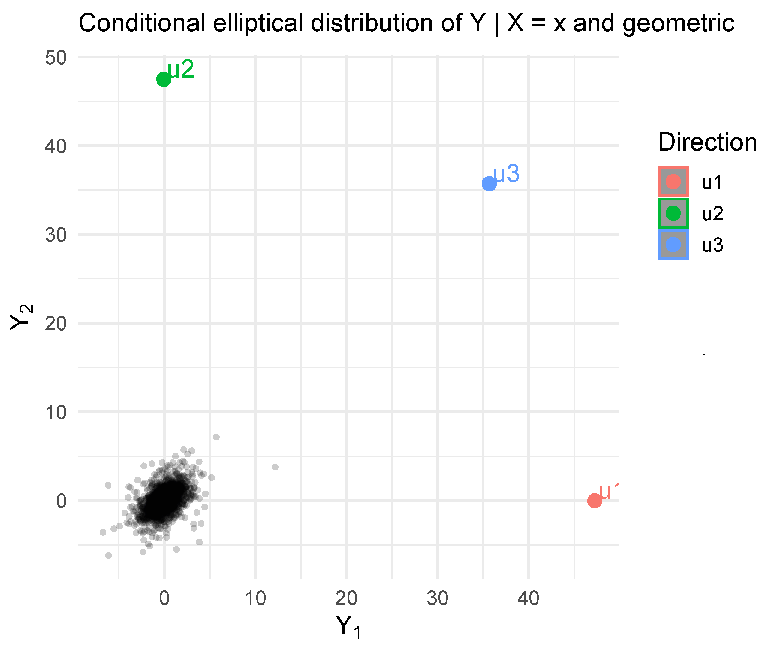
4.4.1. Shape of the Conditional Cloud
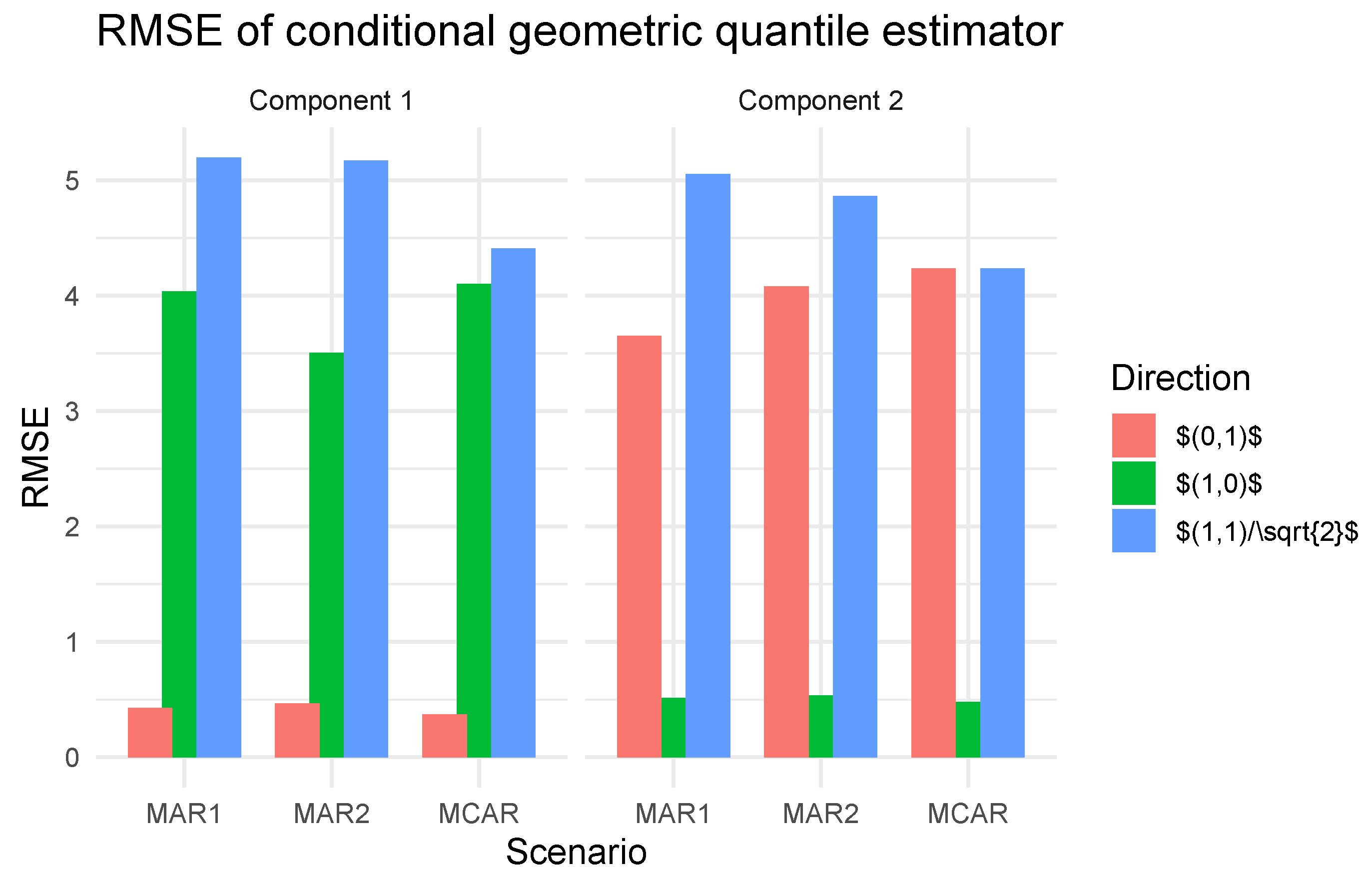
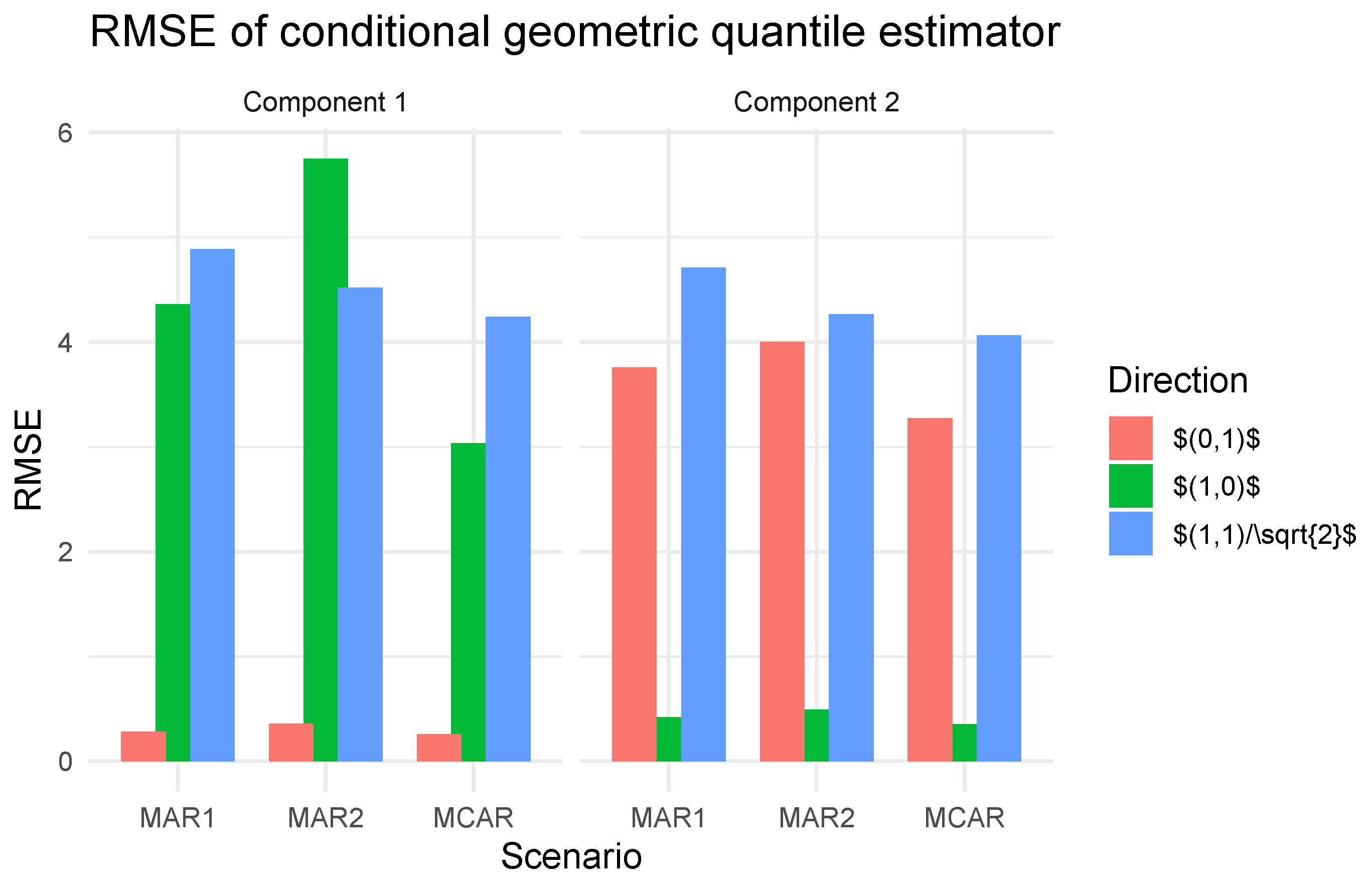
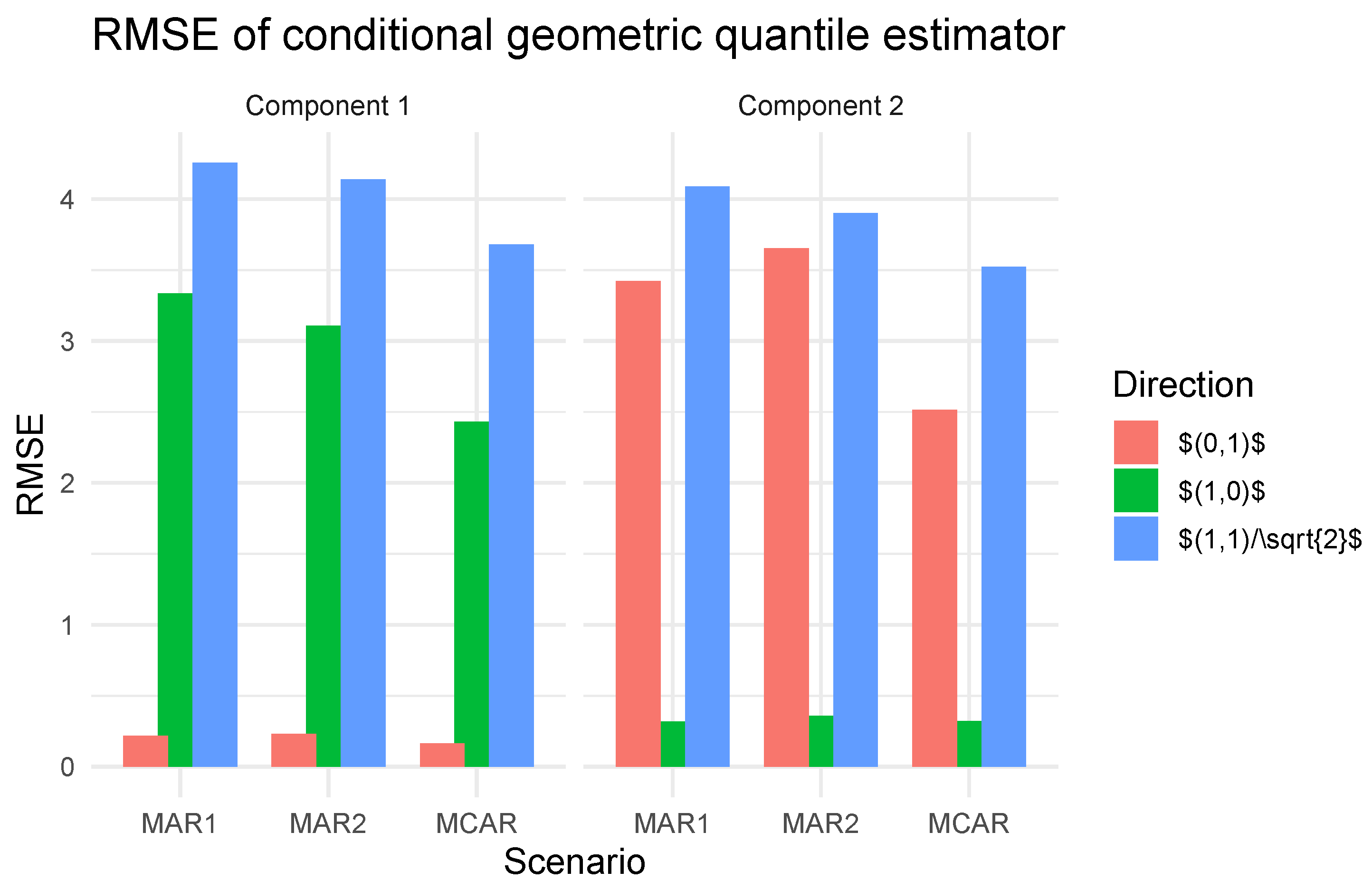
4.4.2. RMSE Behavior
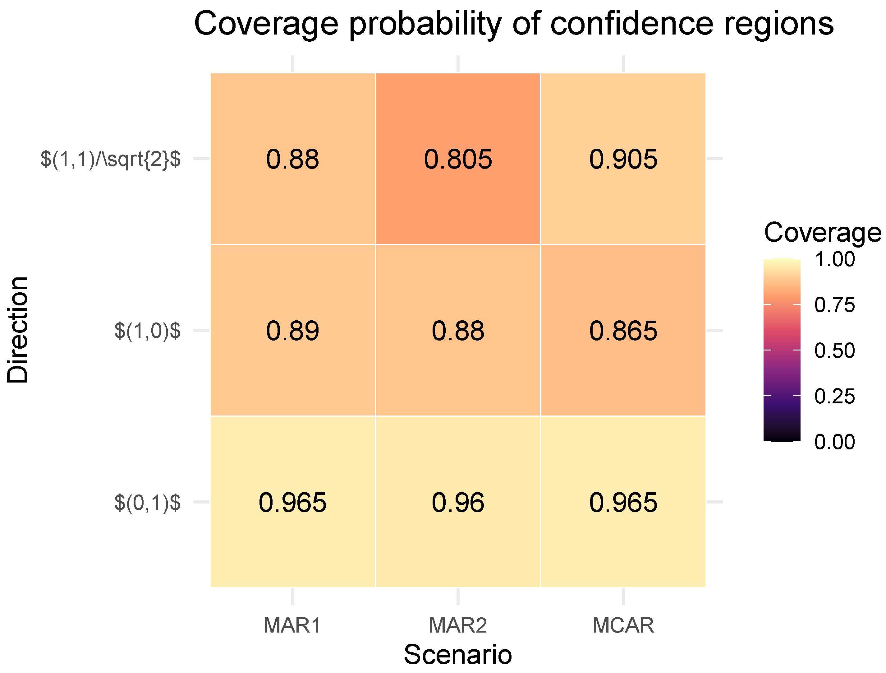
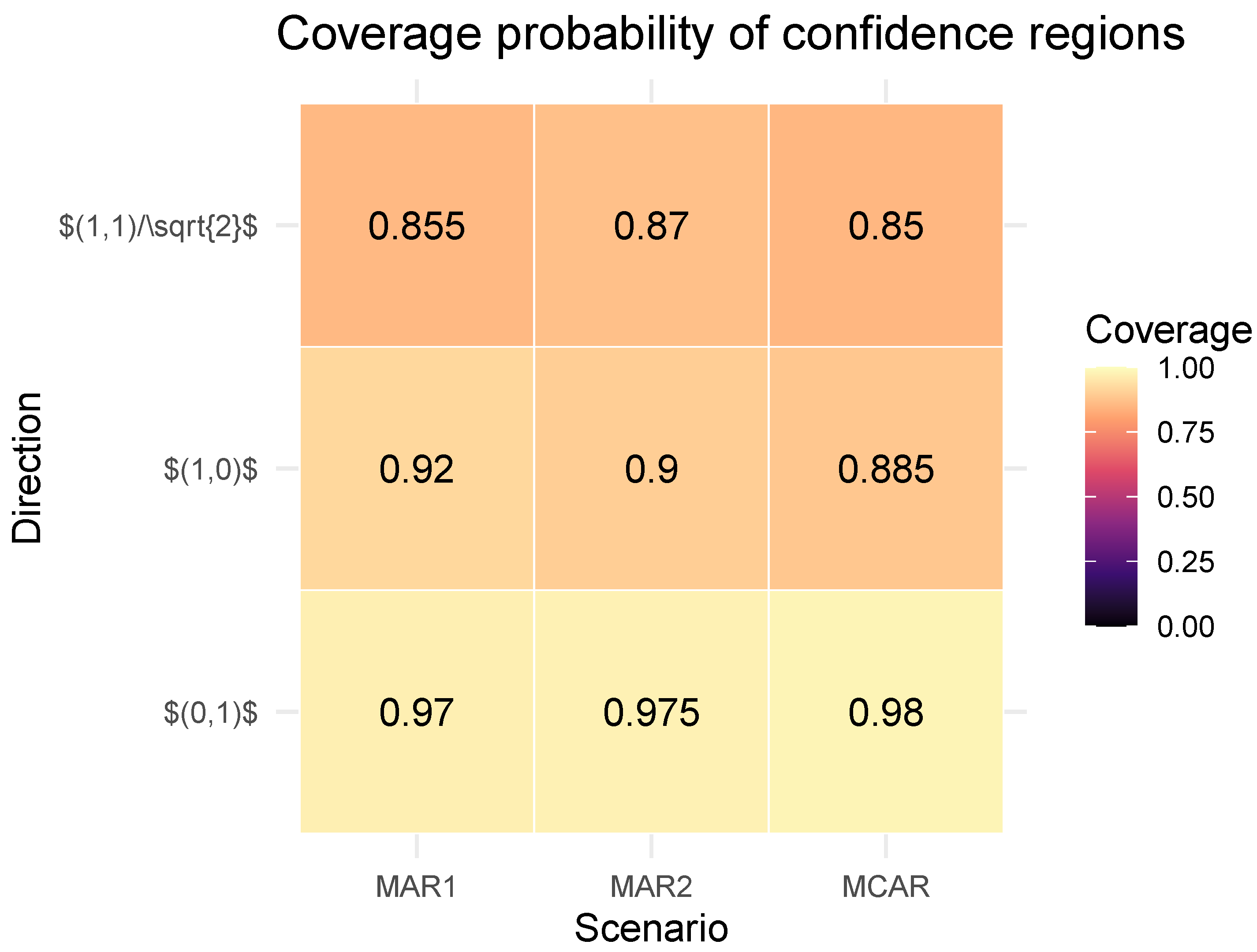
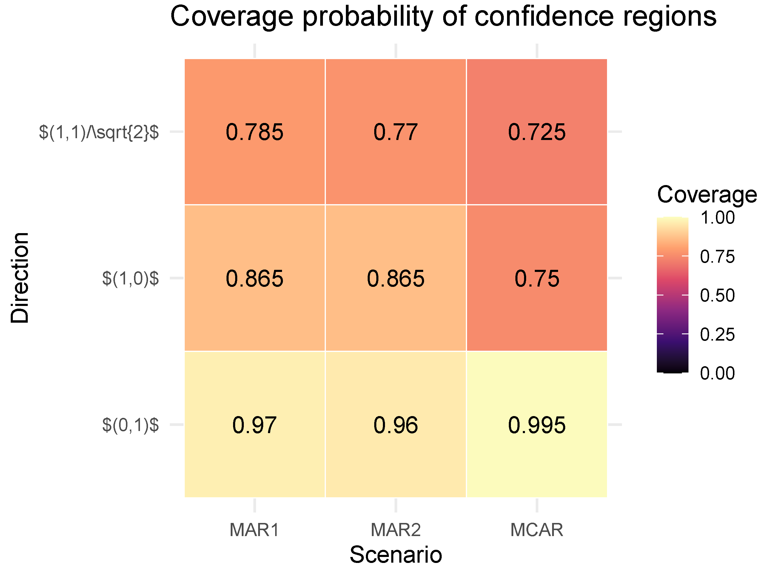
4.4.3. Coverage of Asymptotic Confidence Regions
- For small-to-moderate sample sizes ( and ), coverage is remarkably close to the nominal level for MAR1 and MAR2 in all directions: values range roughly between and , with a slight under-coverage in some MCAR configurations for at and . This indicates that the plug-in variance estimator captures well both the effect of the functional small-ball probability and the MAR correction.
- For the largest sample size the situation becomes more nuanced: MAR2 still displays excellent coverage, often slightly above , while MCAR exhibits noticeable under-coverage in some directions (e.g., coverage around – for and ). This behavior can be traced back to the way the small-ball functionals are estimated: when n grows, the empirical small-ball probability becomes very small under the fixed h selection rule, which makes the variance estimator sensitive to numerical regularization and to the roughness of near its boundary. In practice, this suggests that for very large n one should either let h grow slowly with n or refine the approximation of to stabilise the variance.
- Across directions, coverage is generally slightly better for than for and . This is consistent with the fact that the conditional variance along is more dominated by the noise component and less affected by the non-linear drift, making local quadratic approximations more accurate.
5. Real Data
5.1. Application to Real Blood-Spectroscopy Data
5.2. Data Description and Clinical Context
5.3. Functional Preprocessing and MAR Structure
- 1.
- Identification of functional coordinates. We treat as spectral (functional) coordinates all numeric columns that are neither biomarker targets nor obvious meta-variables (such as IDs and acquisition conditions). Formally, let be the set of indices corresponding to variables such as Reading_ID, donation_id, temperature, and humidity, and let contain the three targets. Then the index set of absorbance wavelengths isand we define as the restriction of the raw observation to coordinates in .
- 2.
- Zero-variance filtering. To avoid degeneracies in the metric and to comply with the small-ball structure of (A2), we remove all spectral coordinates with null empirical variance. Writing for the value of wavelength for individual i, we computeand retain only those wavelengths for which . This is a necessary regularization step in high-dimensional FDA: in the notation of (A2), it prevents the local mass functional from being dominated by degenerate directions and stabilizes the local geometry of the ball .
- 3.
- Per-wavelength centering and scaling. We then standardize the retained spectral channels asso that each wavelength has zero empirical mean and unit (or at least non-zero) variance. This ensures that the semi-metric remains isotropic across wavelengths and that the small-ball probabilities of (A2) and (A3) are not dominated by a few high-energy channels, which would lead to ill-conditioned local neighborhoods and unstable bandwidth selection.
- 4.
- Response and MAR indicator. The bivariate response is constructed asIn this dataset the target variables are essentially fully observed, so that the MAR indicatoris identically equal to one for almost all i. From the point of view of the theory in Section 2, this corresponds to the special case in assumption (A9), so that the MAR correction is neutral. However, all estimation and inference procedures are implemented in their general MAR-robust form, so that the pipeline remains valid for genuinely incomplete panels of biomarkers.
5.4. Choice of Conditioning Point and Bandwidth
- 1.
- We compute the pairwise distances for all , and takethe empirical 15% quantile of the positive distances. This plays the role of a data-driven reference radius in the sense of in (A2).
- 2.
- For each curve , we compute the local MAR-effective massWe then restrict attention to those indices with , which guarantees that the effective local sample size appearing in Proposition 1 and Theorem 3 is sufficiently large.
- 3.
- Among these candidates we define asso that is located in the most densely populated part of the trajectory space (under the MAR-corrected local metric).
5.5. Local Diagnostics for
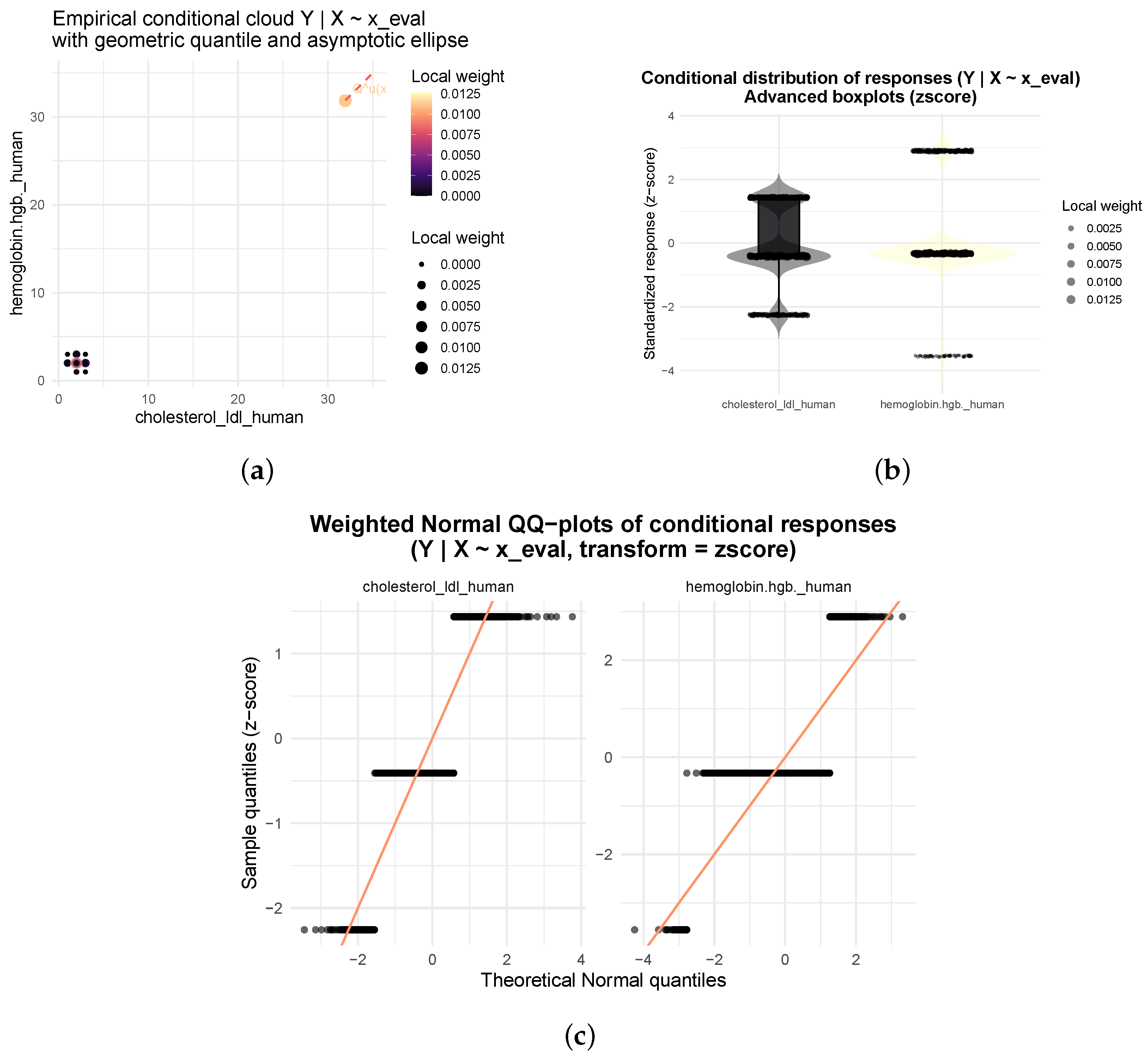
5.6. Directional Conditional Geometric Quantiles
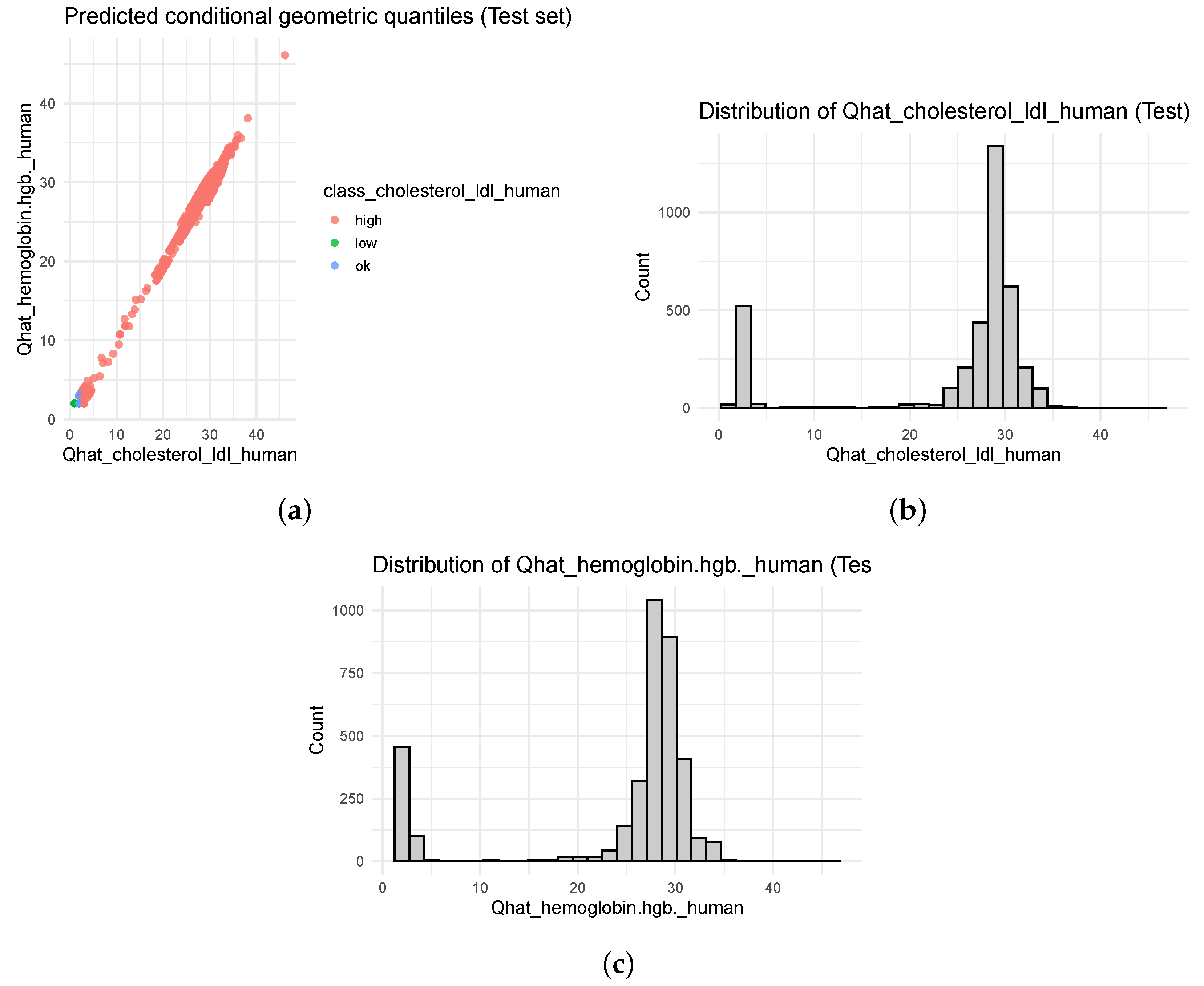
5.7. Out-of-Sample Prediction
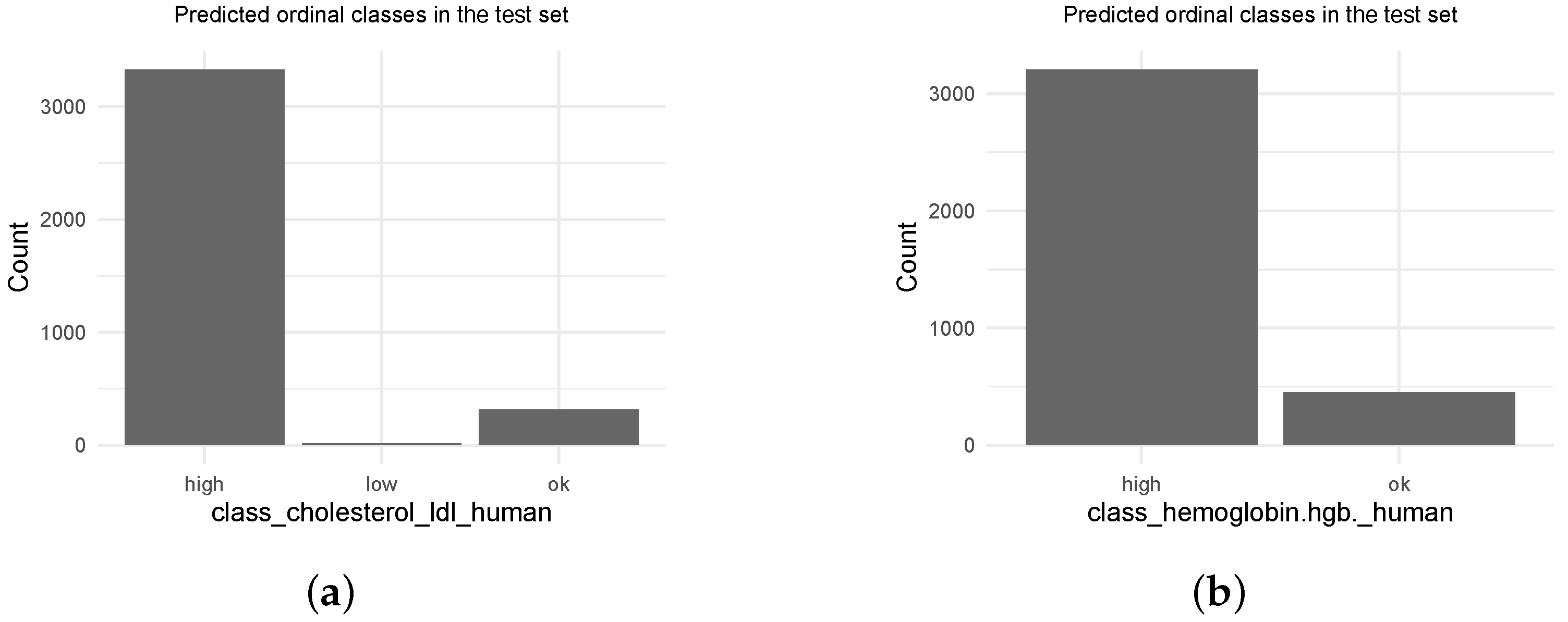
5.8. Ordinal Stratification and Clinical Risk Profiles
5.9. Summary and Perspectives
- The LOOCV bandwidth strategy, although aligned with the geometric loss, could be complemented by a theoretically motivated selector derived from the bias-variance decomposition driven by and in Proposition 1, thereby tightening the link between practice and asymptotic theory.
- The choice of directions u is clinically interpretable; an adaptive scheme (e.g., based on angular sparsity or local tail diagnostics) may uncover latent geometric anisotropies in the conditional law that are not accessible through a priori specified directions.
- Stability of the small-ball behavior could benefit from a preliminary local dimension-reduction step (such as wavelet dictionaries or local FPCA), particularly for spectra with wavelength-dependent heteroscedasticity.
- Since the MAR mechanism in the present dataset is essentially trivial (), a controlled perturbation study or synthetic MAR contamination would illustrate the robustness of the estimator in genuinely incomplete settings and thus emphasize the relevance of assumptions (A4) and (A9).
- Finally, integrating clinical thresholding (e.g., WHO/SFBC hematological ranges) into the ordinal projection could facilitate the translation of geometric quantile diagnostics into operational medical categories.
5.10. The Tecator Data Under MAR
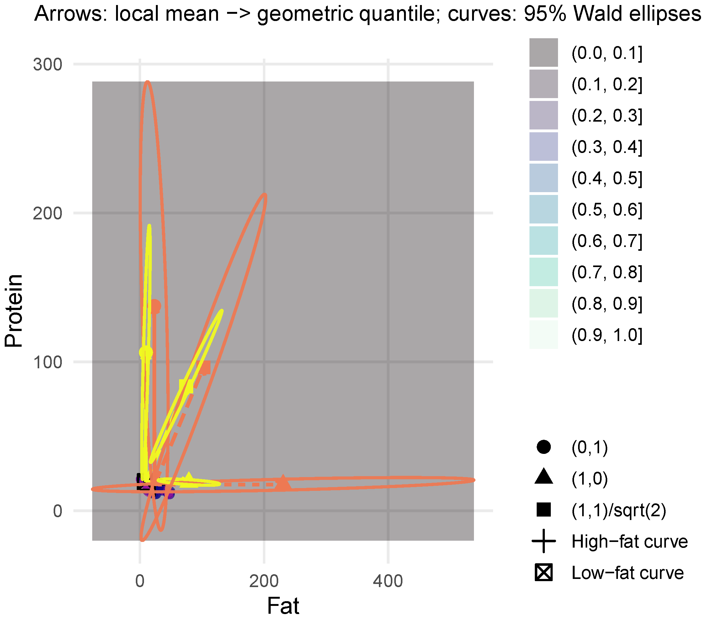
- Main scatter with conditional geometric quantiles: In Figure 12, the joint distribution of is represented via a bivariate density estimate. Local means (with respect to ) at and are marked, and arrows indicate the shift from these means to the estimated conditional geometric quantiles for the different directions u. The associated Wald ellipses are superimposed.
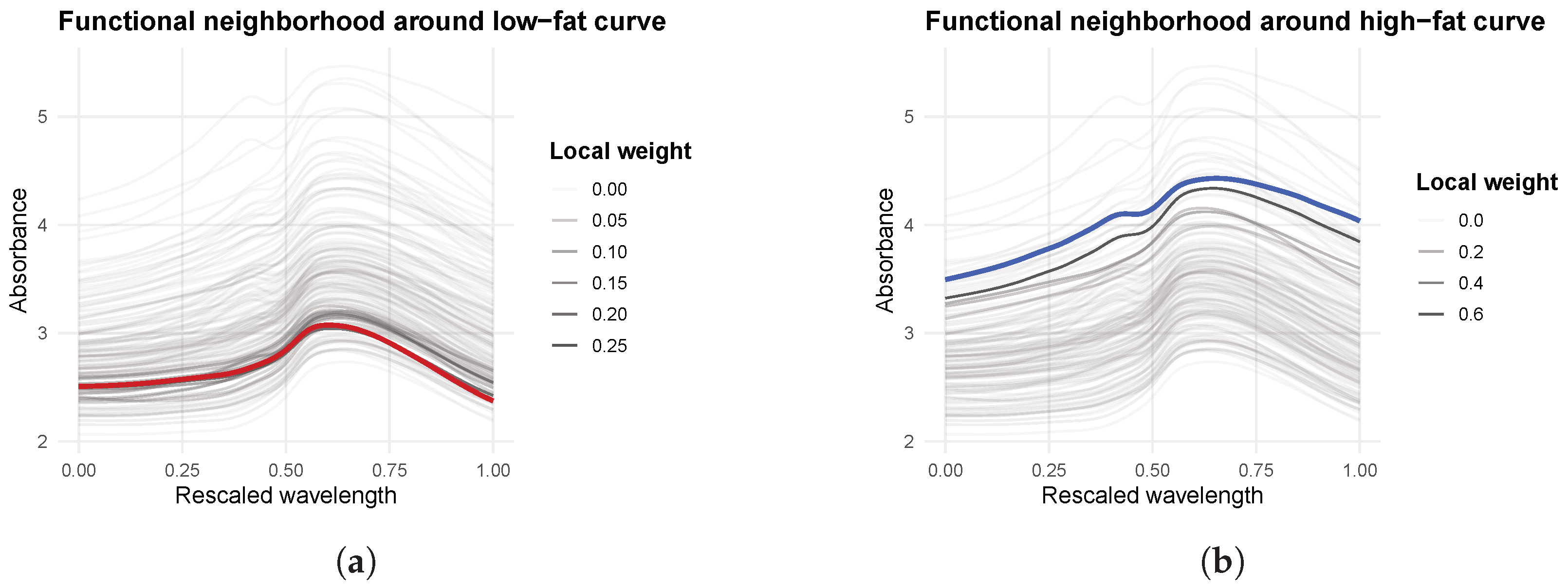
- Functional neighborhoods around the evaluation curves:Figure 13 displays the absorbance curves with transparency proportional to the local weights and , respectively. The evaluation curves and are highlighted, showing how the local neighborhood adapts to the functional geometry.
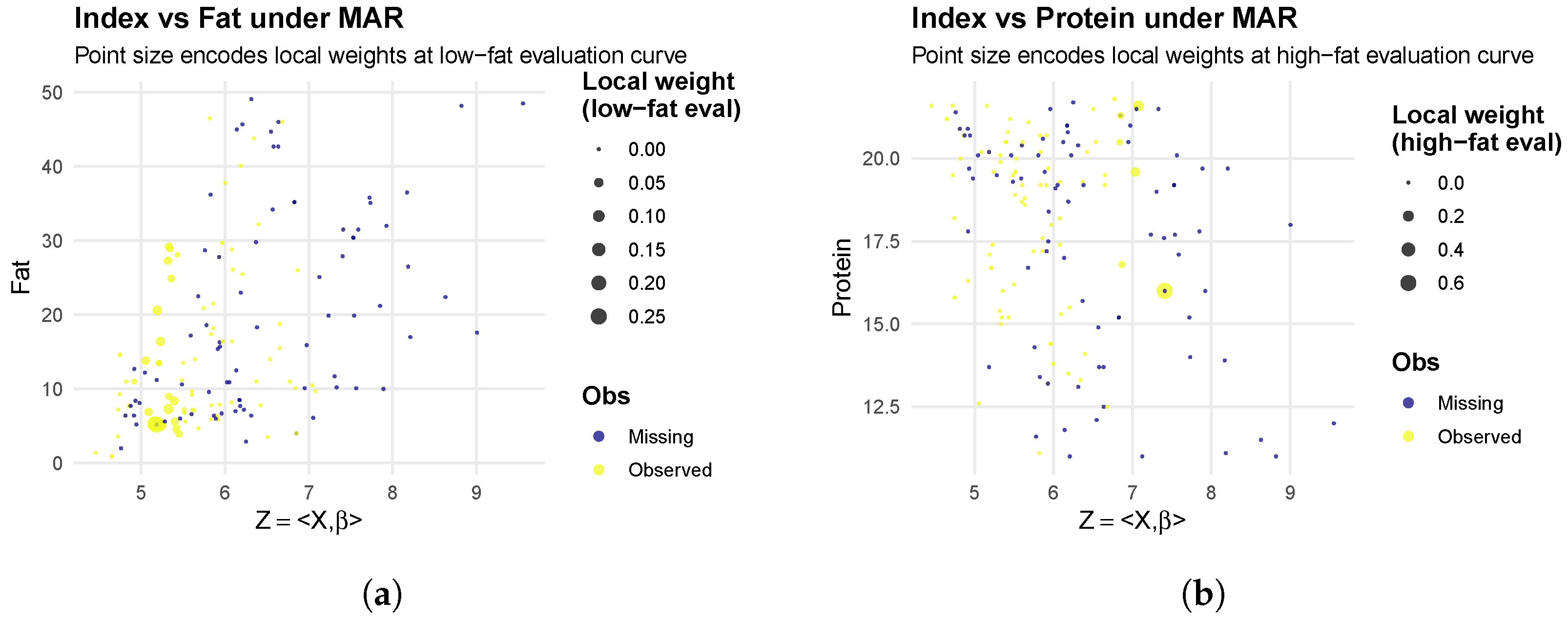
- Index-response plots:Figure 14 shows scatterplots of the scalar index versus Fat and Protein. Points are colored according to the response-availability indicator and their size encodes the local weights at the corresponding evaluation curve. This reveals the MAR pattern and the impact of local weighting.
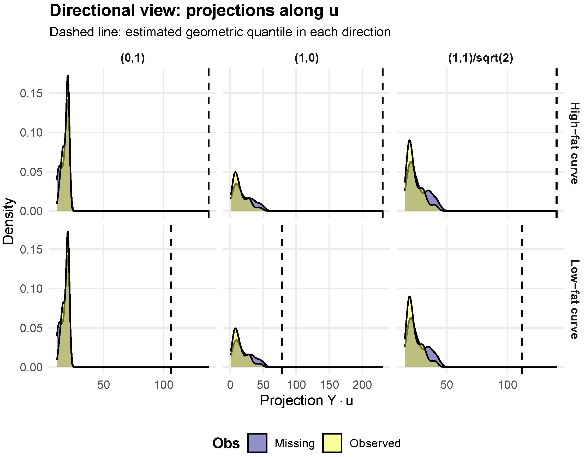
- Directional projections: Finally, Figure 15 reports, for each evaluation point and direction u, the empirical density of the projected responses (distinguishing observed and missing responses) together with a vertical line at the corresponding projected geometric quantile .
6. Concluding Remarks
7. Mathematical Developments
- (i)
- (ii)
- (iii)
- (i)
- (ii)
- (iii)
- we have
- Let such that , the forms a triangular array of stationary martingale differences with respect to the -field . In order to prove Lemma 12, we need to verify the following key conditions:
- (a)
- Conditional variance convergence.
- (b)
- Lindeberg condition [95].holds for any .
Author Contributions
Funding
Data Availability Statement
Acknowledgments
Conflicts of Interest
References
- Ramsay, J.O.; Silverman, B.W. Applied Functional Data Analysis; Springer Series in Statistics; Methods and Case Studies; Springer: New York, NY, USA, 2002; p. x+190. [Google Scholar] [CrossRef]
- Ferraty, F.; Vieu, P. Nonparametric Functional Data Analysis: Theory and Practice; Springer Series in Statistics; Springer: New York, NY, USA, 2006; p. xx+258. [Google Scholar]
- Araujo, A.; Giné, E. The Central Limit Theorem for Real and Banach Valued Random Variables; Wiley Series in Probability and Mathematical Statistics; John Wiley & Sons: New York, NY, USA, 1980; p. xiv+233. [Google Scholar]
- Gasser, T.; Hall, P.; Presnell, B. Nonparametric estimation of the mode of a distribution of random curves. J. R. Stat. Soc. Ser. B Stat. Methodol. 1998, 60, 681–691. [Google Scholar] [CrossRef]
- Bosq, D. Linear Processes in Function Spaces: Theory and Applications; Lecture Notes in Statistics; Springer: New York, NY, USA, 2000; Volume 149, p. xiv+283. [Google Scholar] [CrossRef]
- Horváth, L.; Kokoszka, P. Inference for Functional Data with Applications; Springer Series in Statistics; Springer: New York, NY, USA, 2012; p. xiv+422. [Google Scholar] [CrossRef]
- Kokoszka, P.; Reimherr, M. Introduction to Functional Data Analysis; Texts in Statistical Science Series; CRC Press: Boca Raton, FL, USA, 2017; p. xvi+290. [Google Scholar]
- Ferraty, F.; Laksaci, A.; Tadj, A.; Vieu, P. Rate of uniform consistency for nonparametric estimates with functional variables. J. Stat. Plann. Inference 2010, 140, 335–352. [Google Scholar] [CrossRef]
- Bouzebda, S. On the weak convergence and the uniform-in-bandwidth consistency of the general conditional U-processes based on the copula representation: Multivariate setting. Hacet. J. Math. Stat. 2023, 52, 1303–1348. [Google Scholar] [CrossRef]
- Bouzebda, S. General tests of conditional independence based on empirical processes indexed by functions. Jpn. J. Stat. Data Sci. 2023, 6, 115–177. [Google Scholar] [CrossRef]
- Bouzebda, S.; Nezzal, A. Uniform in number of neighbors consistency and weak convergence of kNN empirical conditional processes and kNN conditional U-processes involving functional mixing data. AIMS Math. 2024, 9, 4427–4550. [Google Scholar] [CrossRef]
- Bouzebda, S.; Nezzal, A. Uniform consistency and uniform in number of neighbors consistency for nonparametric regression estimates and conditional U-statistics involving functional data. Jpn. J. Stat. Data Sci. 2022, 5, 431–533. [Google Scholar] [CrossRef]
- Kara-Zaitri, L.; Laksaci, A.; Rachdi, M.; Vieu, P. Uniform in bandwidth consistency for various kernel estimators involving functional data. J. Nonparametr. Stat. 2017, 29, 85–107. [Google Scholar] [CrossRef]
- Attouch, M.; Laksaci, A.; Rafaa, F. On the local linear estimate for functional regression: Uniform in bandwidth consistency. Comm. Stat. Theory Methods 2019, 48, 1836–1853. [Google Scholar] [CrossRef]
- Chen, C.X.; Ling, N.X.; Ling, J.; Liu, Y. Convergence rate of nonparametric recursive M-estimation for functional stationary ergodic data. J. Hefei Univ. Technol. Nat. Sci. 2019, 42, 710–714. [Google Scholar]
- Mohammedi, M.; Bouzebda, S.; Laksaci, A. The consistency and asymptotic normality of the kernel type expectile regression estimator for functional data. J. Multivar. Anal. 2021, 181, 104673. [Google Scholar] [CrossRef]
- Bouzebda, S.; Laksaci, A.; Mohammedi, M. Single index regression model for functional quasi-associated time series data. REVSTAT Stat. J. 2022, 20, 605–631. [Google Scholar]
- Bouzebda, S.; Laksaci, A.; Mohammedi, M. The k-nearest neighbors method in single index regression model for functional quasi-associated time series data. Rev. Mat. Complut. 2023, 36, 361–391. [Google Scholar] [CrossRef]
- Agua, B.M.; Bouzebda, S. Single index regression for locally stationary functional time series. AIMS Math. 2024, 9, 36202–36258. [Google Scholar] [CrossRef]
- Bouanani, O.; Bouzebda, S. Limit theorems for local polynomial estimation of regression for functional dependent data. AIMS Math. 2024, 9, 23651–23691. [Google Scholar] [CrossRef]
- Bouzebda, S. Weak convergence of the conditional single index U-statistics for locally stationary functional time series. AIMS Math. 2024, 9, 14807–14898. [Google Scholar] [CrossRef]
- Bouzebda, S. Limit Theorems in the Nonparametric Conditional Single-Index U-Processes for Locally Stationary Functional Random Fields under Stochastic Sampling Design. Mathematics 2024, 12, 1996. [Google Scholar] [CrossRef]
- Bouzebda, S. Uniform in Number of Neighbor Consistency and Weak Convergence of k-Nearest Neighbor Single Index Conditional Processes and k-Nearest Neighbor Single Index Conditional U-Processes Involving Functional Mixing Data. Symmetry 2024, 16, 1576. [Google Scholar] [CrossRef]
- Bouzebda, S.; Soukarieh, I. Non-Parametric Conditional U-Processes for Locally Stationary Functional Random Fields under Stochastic Sampling Design. Mathematics 2023, 11, 16. [Google Scholar] [CrossRef]
- Lestari, B.; Chamidah, N.; Nyoman Budiantara, I.; Aydin, D. Determining confidence interval and asymptotic distribution for parameters of multiresponse semiparametric regression model using smoothing spline estimator. J. King Saud Univ. Sci. 2023, 35, 102664. [Google Scholar] [CrossRef]
- Chamidah, N.; Lestari, B.; Budiantara, I.N.; Saifudin, T.; Rulaningtyas, R.; Aryati, A.; Wardani, P.; Aydin, D. Consistency and Asymptotic Normality of Estimator for Parameters in Multiresponse Multipredictor Semiparametric Regression Model. Symmetry 2022, 14, 336. [Google Scholar] [CrossRef]
- Koenker, R.; Bassett, G., Jr. Regression quantiles. Econometrica 1978, 46, 33–50. [Google Scholar] [CrossRef]
- Koenker, R. Econometric Society Monographs. In Quantile Regression; Cambridge University Press: Cambridge, UK, 2005; Volume 38, p. xvi+349. [Google Scholar] [CrossRef]
- Kong, D.; Maity, A.; Hsu, F.C.; Tzeng, J.Y. Testing and estimation in marker-set association study using semiparametric quantile regression kernel machine. Biometrics 2016, 72, 364–371. [Google Scholar] [CrossRef]
- Kato, K. Estimation in functional linear quantile regression. Ann. Stat. 2012, 40, 3108–3136. [Google Scholar] [CrossRef]
- Lu, Y.; Du, J.; Sun, Z. Functional partially linear quantile regression model. Metrika 2014, 77, 317–332. [Google Scholar] [CrossRef]
- Yu, P.; Du, J.; Zhang, Z. Varying-coefficient partially functional linear quantile regression models. J. Korean Stat. Soc. 2017, 46, 462–475. [Google Scholar] [CrossRef]
- Du, J.; Zhang, Z.; Sun, Z. Variable selection for partially linear varying coefficient quantile regression model. Int. J. Biomath. 2013, 6, 1350015. [Google Scholar] [CrossRef]
- Xu, D.; Du, J. Nonparametric quantile regression estimation for functional data with responses missing at random. Metrika 2020, 83, 977–990. [Google Scholar] [CrossRef]
- Rubin, D.B. Inference and missing data. Biometrika 1976, 63, 581–592. [Google Scholar] [CrossRef]
- Little, R.J.A.; Rubin, D.B. Statistical Analysis with Missing Data, 2nd ed.; Wiley Series in Probability and Statistics; John Wiley & Sons: Hoboken, NJ, USA, 2002; p. xviii+381. [Google Scholar] [CrossRef]
- Josse, J.; Reiter, J.P. Introduction to the special section on missing data. Stat. Sci. 2018, 33, 139–141. [Google Scholar] [CrossRef]
- Claeskens, G.; Hjort, N.L. Model Selection and Model Averaging; Cambridge Series in Statistical and Probabilistic Mathematics; Cambridge University Press: Cambridge, UK, 2008; Volume 27, p. xviii+312. [Google Scholar] [CrossRef]
- Seaman, S.; Galati, J.; Jackson, D.; Carlin, J. What is meant by “missing at random”? Stat. Sci. 2013, 28, 257–268. [Google Scholar] [CrossRef]
- Mealli, F.; Rubin, D.B. Clarifying missing at random and related definitions, and implications when coupled with exchangeability. Biometrika 2015, 102, 995–1000. [Google Scholar] [CrossRef]
- Doretti, M.; Geneletti, S.; Stanghellini, E. Missing data: A unified taxonomy guided by conditional independence. Int. Stat. Rev. 2018, 86, 189–204. [Google Scholar] [CrossRef]
- Bouzebda, S.; Taachouche, N. Limit theorems for conditional U-statistics analysis on hyperspheres for missing at random data in the presence of measurement error. J. Comput. Appl. Math. 2026, 472, 116811. [Google Scholar] [CrossRef]
- Abdous, B.; Theodorescu, R. Note on the spatial quantile of a random vector. Stat. Probab. Lett. 1992, 13, 333–336. [Google Scholar] [CrossRef]
- Chaudhuri, P. On a geometric notion of quantiles for multivariate data. J. Am. Stat. Assoc. 1996, 91, 862–872. [Google Scholar] [CrossRef]
- Hallin, M.; Paindaveine, D.; Šiman, M. Multivariate quantiles and multiple-output regression quantiles: From L1 optimization to halfspace depth. Ann. Stat. 2010, 38, 635–669. [Google Scholar] [CrossRef]
- Koltchinskii, V.I. M-estimation, convexity and quantiles. Ann. Stat. 1997, 25, 435–477. [Google Scholar] [CrossRef]
- Liu, R.Y.; Parelius, J.M.; Singh, K. Multivariate analysis by data depth: Descriptive statistics, graphics and inference (with discussion and a rejoinder by Liu and Singh). Ann. Stat. 1999, 27, 783–858. [Google Scholar] [CrossRef]
- Hlávka, Z.; Hlubinka, D.; Hudecová, V. Multivariate quantile-based permutation tests with application to functional data. J. Comput. Graph. Stat. 2025, 34, 1276–1290. [Google Scholar] [CrossRef]
- Bernard, C.; Perchiazzo, A.; Vanduffel, S. Multivariate portfolio choice via quantiles. Quant. Finance 2026, 26, 15–39. [Google Scholar] [CrossRef]
- Hlubinka, D.; Kotík, L.; Šiman, M. Multivariate quantiles with both overall and directional probability interpretation. Scand. J. Stat. 2022, 49, 1586–1604. [Google Scholar] [CrossRef]
- Llorens-Terrazas, J. An oracle inequality for multivariate dynamic quantile forecasting. J. Bus. Econ. Stat. 2025, 43, 603–614. [Google Scholar] [CrossRef]
- Shin, H.Y.; Oh, H.S. Geometric quantile-based measures of multivariate distributional characteristics. Stat. Probab. Lett. 2025, 219, 110325. [Google Scholar] [CrossRef]
- Bhattacharya, I.; Ghosal, S. Bayesian multivariate quantile regression using dependent Dirichlet process prior. J. Multivariate Anal. 2021, 185, 104763. [Google Scholar] [CrossRef]
- Berlinet, A.; Cadre, B.; Gannoun, A. On the conditional L1-median and its estimation. J. Nonparametr. Stat. 2001, 13, 631–645. [Google Scholar] [CrossRef]
- Cadre, B.; Gannoun, A. Asymptotic normality of consistent estimate of the conditional L1-median. Ann. ISUP 2000, 44, 13–33. [Google Scholar]
- Cheng, Y.; De Gooijer, J.G. On the uth geometric conditional quantile. J. Stat. Plann. Inference 2007, 137, 1914–1930. [Google Scholar] [CrossRef]
- De Gooijer, J.G.; Gannoun, A.; Zerom, D. A multivariate quantile predictor. Comm. Stat. Theory Methods 2006, 35, 133–147. [Google Scholar] [CrossRef]
- Bouzebda, S.; Taachouche, N. Multivariate spatial conditional U-quantiles: A Bahadur–Kiefer representation. Results Appl. Math. 2025, 26, 100593. [Google Scholar] [CrossRef]
- Chaouch, M.; Laïb, N. Nonparametric multivariate L1-median regression estimation with functional covariates. Electron. J. Stat. 2013, 7, 1553–1586. [Google Scholar] [CrossRef]
- Ramsay, J.O.; Silverman, B.W. Functional Data Analysis, 2nd ed.; Springer Series in Statistics; Springer: New York, NY, USA, 2005; p. xx+426. [Google Scholar]
- Ezzahrioui, M.; Ould Saïd, E. Some asymptotic results of a non-parametric conditional mode estimator for functional time-series data. Stat. Neerl. 2010, 64, 171–201. [Google Scholar] [CrossRef]
- Masry, E. Nonparametric regression estimation for dependent functional data: Asymptotic normality. Stoch. Process. Appl. 2005, 115, 155–177. [Google Scholar] [CrossRef]
- Rosenblatt, M. Uniform ergodicity and strong mixing. Z. Wahrscheinlichkeitstheorie Verw. Geb. 1972, 24, 79–84. [Google Scholar] [CrossRef]
- Andrews, D.W.K. Non-strong mixing autoregressive processes. J. Appl. Probab. 1984, 21, 930–934. [Google Scholar] [CrossRef]
- Bouzebda, S.; Didi, S.; El Hajj, L. Multivariate wavelet density and regression estimators for stationary and ergodic continuous time processes: Asymptotic results. Math. Methods Stat. 2015, 24, 163–199. [Google Scholar] [CrossRef]
- Bouzebda, S.; Chaouch, M.; Didi Biha, S. Asymptotics for function derivatives estimators based on stationary and ergodic discrete time processes. Ann. Inst. Stat. Math. 2022, 74, 737–771. [Google Scholar] [CrossRef]
- Laïb, N.; Ould-Saïd, E. A robust nonparametric estimation of the autoregression function under an ergodic hypothesis. Canad. J. Stat. 2000, 28, 817–828. [Google Scholar] [CrossRef][Green Version]
- Bouzebda, S.; Didi, S. Additive regression model for stationary and ergodic continuous time processes. Comm. Stat. Theory Methods 2017, 46, 2454–2493. [Google Scholar] [CrossRef]
- Bouzebda, S.; Didi, S. Some asymptotic properties of kernel regression estimators of the mode for stationary and ergodic continuous time processes. Rev. Mat. Complut. 2021, 34, 811–852. [Google Scholar] [CrossRef]
- Bouzebda, S.; Didi, S. Some results about kernel estimators for function derivatives based on stationary and ergodic continuous time processes with applications. Comm. Stat. Theory Methods 2022, 51, 3886–3933. [Google Scholar] [CrossRef]
- Bouzebda, S.; Chaouch, M. Uniform limit theorems for a class of conditional Z-estimators when covariates are functions. J. Multivar. Anal. 2022, 189, 104872. [Google Scholar] [CrossRef]
- Chaouch, M.; Laïb, N. Regression estimation for continuous-time functional data processes with missing at random response. J. Nonparametr. Stat. 2025, 37, 1–32. [Google Scholar] [CrossRef]
- Giraitis, L.; Leipus, R. A generalized fractionally differencing approach in long-memory modeling. Liet. Mat. Rink. 1995, 35, 65–81. [Google Scholar] [CrossRef]
- Guégan, D.; Ladoucette, S. Non-mixing properties of long memory processes. C. R. Acad. Sci. Paris Sér. I Math. 2001, 333, 373–376. [Google Scholar] [CrossRef]
- Francq, C.; Zakoïan, J.M. GARCH Models: Structure, Statistical Inference and Financial Applications; John Wiley & Sons, Ltd.: Chichester, UK, 2010; p. xiv+489. [Google Scholar] [CrossRef]
- Dang, X.; Serfling, R. Nonparametric depth-based multivariate outlier identifiers, and masking robustness properties. J. Stat. Plann. Inference 2010, 140, 198–213. [Google Scholar] [CrossRef]
- Mazumder, S.; Serfling, R. A robust sample spatial outlyingness function. J. Stat. Plann. Inference 2013, 143, 144–159. [Google Scholar] [CrossRef]
- Konen, D.; Paindaveine, D. On the robustness of spatial quantiles. Ann. Inst. Henri Poincaré Probab. Stat. 2026, 62, 548–581. [Google Scholar] [CrossRef]
- Altukhaes, W.B.; Roozbeh, M.; Mohamed, N.A. Robust Liu Estimator Used to Combat Some Challenges in Partially Linear Regression Model by Improving LTS Algorithm Using Semidefinite Programming. Mathematics 2024, 12, 2787. [Google Scholar] [CrossRef]
- Hsing, T.; Eubank, R. Theoretical Foundations of Functional Data Analysis, with an Introduction to Linear Operators; Wiley Series in Probability and Statistics; John Wiley & Sons, Ltd.: Chichester, UK, 2015; p. xiv+334. [Google Scholar] [CrossRef]
- Yao, W. A bias corrected nonparametric regression estimator. Stat. Probab. Lett. 2012, 82, 274–282. [Google Scholar] [CrossRef]
- Karlsson, A. Bootstrap methods for bias correction and confidence interval estimation for nonlinear quantile regression of longitudinal data. J. Stat. Comput. Simul. 2009, 79, 1205–1218. [Google Scholar] [CrossRef]
- Didi, S.; Bouzebda, S. Wavelet Density and Regression Estimators for Continuous Time Functional Stationary and Ergodic Processes. Mathematics 2022, 10, 4356. [Google Scholar] [CrossRef]
- Didi, S.; Al Harby, A.; Bouzebda, S. Wavelet Density and Regression Estimators for Functional Stationary and Ergodic Data: Discrete Time. Mathematics 2022, 10, 3433. [Google Scholar] [CrossRef]
- Bouzebda, S.; Nezzal, A. Asymptotic properties of conditional U-statistics using delta sequences. Comm. Stat. Theory Methods 2024, 53, 4602–4657. [Google Scholar] [CrossRef]
- Cheng, M.Y.; Wu, H.T. Local linear regression on manifolds and its geometric interpretation. J. Amer. Stat. Assoc. 2013, 108, 1421–1434. [Google Scholar] [CrossRef]
- de la Peña, V.H.; Giné, E. Decoupling: From Dependence to Independence; Randomly Stopped Processes U-Statistics and Processes Martingales and Beyond; Probability and Its Applications; Springer: New York, NY, USA, 1999; p. xvi+392. [Google Scholar] [CrossRef]
- Laib, N.; Louani, D. Nonparametric kernel regression estimation for functional stationary ergodic data: Asymptotic properties. J. Multivariate Anal. 2010, 101, 2266–2281. [Google Scholar] [CrossRef]
- Burkholder, D.L. The best constant in the Davis inequality for the expectation of the martingale square function. Trans. Amer. Math. Soc. 2002, 354, 91–105. [Google Scholar] [CrossRef]
- Davis, B. On the integrability of the martingale square function. Israel J. Math. 1970, 8, 187–190. [Google Scholar] [CrossRef]
- Burkholder, D.L.; Gundy, R.F. Extrapolation and interpolation of quasi-linear operators on martingales. Acta Math. 1970, 124, 249–304. [Google Scholar] [CrossRef]
- Hall, P.; Heyde, C.C. Martingale Limit Theory and Its Application; Probability and Mathematical Statistics; Academic Press, Inc.: London, UK, 1980; p. xii+308. [Google Scholar]
- Azuma, K. Weighted sums of certain dependent random variables. Tohoku Math. J. 1967, 19, 357–367. [Google Scholar] [CrossRef]
- Hoeffding, W. Probability inequalities for sums of bounded random variables. J. Amer. Stat. Assoc. 1963, 58, 13–30. [Google Scholar] [CrossRef]
- Lindeberg, J.W. Eine neue Herleitung des Exponentialgesetzes in der Wahrscheinlichkeitsrechnung. Math. Z. 1922, 15, 211–225. [Google Scholar] [CrossRef]



| Symbol | Meaning |
|---|---|
| (X,Y) | Random element taking values in |
| E | Semi-metric functional covariate space (e.g., Hilbert or Banach space) |
| d(x,) | Semi-metric measuring distance between curves in E |
| Euclidean inner product in | |
| Euclidean norm in | |
| Unit ball | |
| Strictly stationary ergodic sequence of observations | |
| Sigma-field generated by past observations up to time i | |
| Sigma-field generated by past observations and | |
| Shift operator of the underlying stochastic process | |
| Small-ball probability | |
| (h) | Conditional small-ball probability given |
| (h) | Rate function such that as |
| Leading term in the small-ball expansion | |
| (s) | Limit ratio as |
| Meaning | |
|---|---|
| u | Direction parameter in defining the geometric quantile |
| m | Candidate location vector in |
| Geometric quantile loss | |
| Conditional risk | |
| Conditional geometric quantile | |
| Gradient of the conditional risk with respect to m | |
| Hessian matrix of | |
| Subgradient of : | |
| Local curvature matrix of the geometric loss | |
| Conditional covariance matrix of given |
| Meaning | |
|---|---|
| Kernel function supported on | |
| Bandwidth parameter with as | |
| Kernel weight | |
| Nadaraya–Watson weight (complete data) | |
| MAR-corrected Nadaraya–Watson weight | |
| Kernel estimator of | |
| MAR-weighted kernel estimator of | |
| Kernel estimator of (complete data) | |
| Kernel estimator under MAR | |
| Response indicator (1 if observed) | |
| Response probability | |
| Kernel estimator of | |
| Empirical small-ball probability | |
| Kernel small-ball constants in asymptotic variance | |
| Asymptotic covariance matrix of |
| Scenario | Direction | Bias | RMSE | Coverage | |||
|---|---|---|---|---|---|---|---|
| 250 | MCAR | 1.027 | 0.311 | 4.100 | 0.481 | 0.865 | |
| 0.018 | 1.554 | 0.373 | 4.236 | 0.965 | |||
| −3.356 | −3.089 | 4.410 | 4.235 | 0.905 | |||
| MAR1 | 0.206 | 0.317 | 4.035 | 0.515 | 0.890 | ||
| 0.018 | 0.859 | 0.428 | 3.650 | 0.965 | |||
| −3.460 | −3.140 | 5.197 | 5.053 | 0.880 | |||
| MAR2 | −0.695 | 0.265 | 3.504 | 0.537 | 0.880 | ||
| −0.026 | 0.499 | 0.467 | 4.079 | 0.960 | |||
| −3.727 | −3.336 | 5.169 | 4.861 | 0.805 | |||
| 500 | MCAR | 0.791 | 0.232 | 3.035 | 0.353 | 0.885 | |
| −0.026 | 1.308 | 0.259 | 3.275 | 0.980 | |||
| −2.945 | −2.667 | 4.241 | 4.064 | 0.850 | |||
| MAR1 | 1.420 | 0.260 | 4.362 | 0.420 | 0.920 | ||
| −0.024 | 1.246 | 0.280 | 3.760 | 0.970 | |||
| −3.412 | -3.145 | 4.889 | 4.710 | 0.855 | |||
| MAR2 | 0.570 | 0.288 | 5.749 | 0.490 | 0.900 | ||
| −0.063 | 1.273 | 0.360 | 4.004 | 0.975 | |||
| −3.331 | −2.992 | 4.519 | 4.263 | 0.870 | |||
| 1000 | MCAR | 0.775 | 0.275 | 2.432 | 0.322 | 0.750 | |
| −0.006 | 1.249 | 0.163 | 2.516 | 0.995 | |||
| −2.269 | −2.005 | 3.681 | 3.524 | 0.725 | |||
| MAR1 | 1.230 | 0.239 | 3.335 | 0.319 | 0.865 | ||
| −0.024 | 1.346 | 0.217 | 3.424 | 0.970 | |||
| −2.833 | −2.571 | 4.258 | 4.089 | 0.785 | |||
| MAR2 | 0.812 | 0.283 | 3.108 | 0.358 | 0.865 | ||
| −0.074 | 1.576 | 0.230 | 3.655 | 0.960 | |||
| −3.177 | −2.861 | 4.140 | 3.902 | 0.770 | |||
| Direction | ||
|---|---|---|
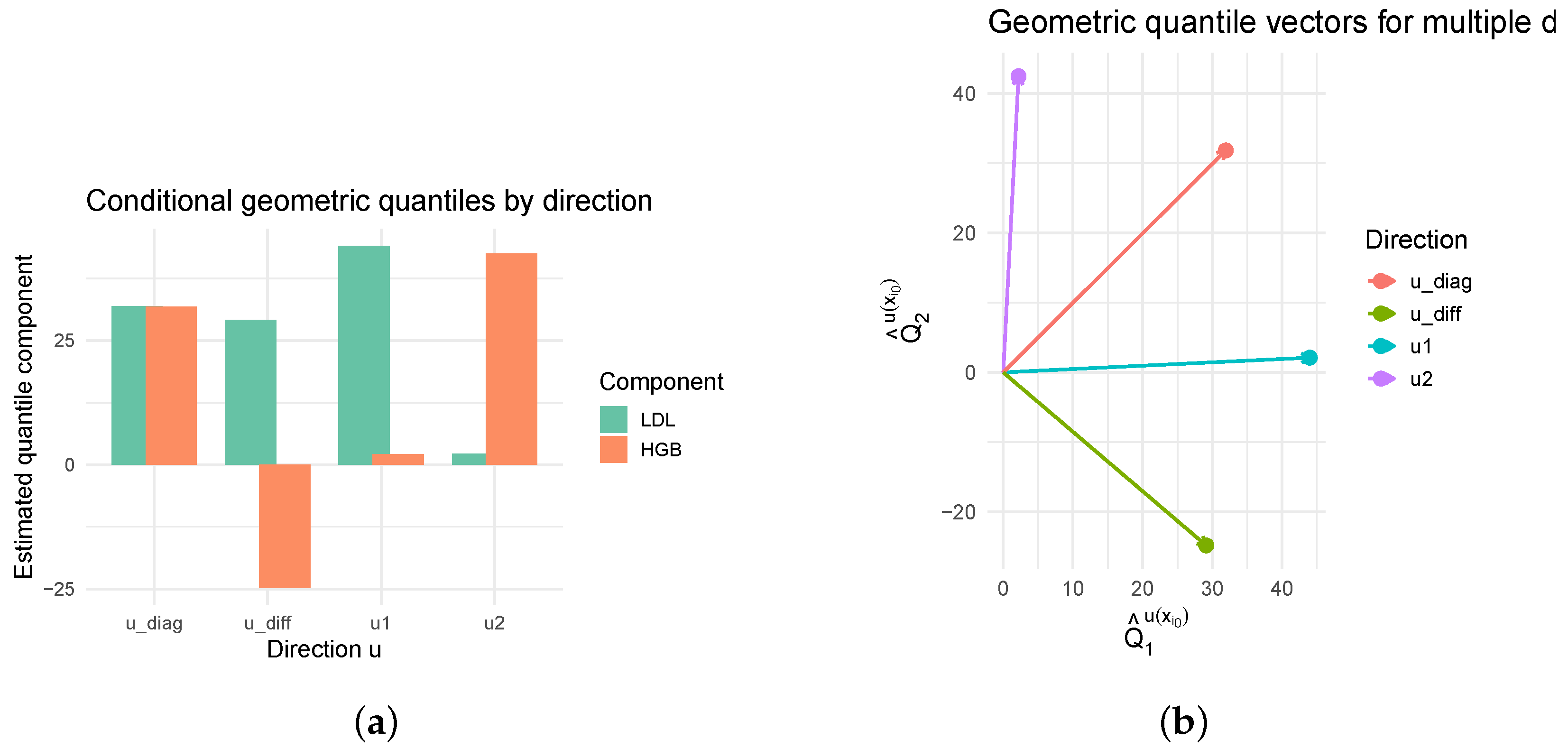
| u1 | 44.00 | 2.11 |
| u2 | 2.20 | 42.46 |
| u_diag | 31.93 | 31.83 |
| u_diff | 29.11 | −24.81 |
Disclaimer/Publisher’s Note: The statements, opinions and data contained in all publications are solely those of the individual author(s) and contributor(s) and not of MDPI and/or the editor(s). MDPI and/or the editor(s) disclaim responsibility for any injury to people or property resulting from any ideas, methods, instructions or products referred to in the content. |
© 2026 by the authors. Licensee MDPI, Basel, Switzerland. This article is an open access article distributed under the terms and conditions of the Creative Commons Attribution (CC BY) license.
Share and Cite
Belhas, H.; Mohammedi, M.; Bouzebda, S. Asymptotic Theory for Multivariate Nonparametric Quantile Regression with Stationary Ergodic Functional Covariates and Missing-at-Random Responses. Symmetry 2026, 18, 445. https://doi.org/10.3390/sym18030445
Belhas H, Mohammedi M, Bouzebda S. Asymptotic Theory for Multivariate Nonparametric Quantile Regression with Stationary Ergodic Functional Covariates and Missing-at-Random Responses. Symmetry. 2026; 18(3):445. https://doi.org/10.3390/sym18030445
Chicago/Turabian StyleBelhas, Hadjer, Mustapha Mohammedi, and Salim Bouzebda. 2026. "Asymptotic Theory for Multivariate Nonparametric Quantile Regression with Stationary Ergodic Functional Covariates and Missing-at-Random Responses" Symmetry 18, no. 3: 445. https://doi.org/10.3390/sym18030445
APA StyleBelhas, H., Mohammedi, M., & Bouzebda, S. (2026). Asymptotic Theory for Multivariate Nonparametric Quantile Regression with Stationary Ergodic Functional Covariates and Missing-at-Random Responses. Symmetry, 18(3), 445. https://doi.org/10.3390/sym18030445