Bonferroni Mean Operators on Weighted Hesitant Fuzzy Set and Its Application in Multi-Criteria Symmetric Group Decision Making

Abstract

The Bonferroni mean operator, as a powerful aggregation operator, is widely applied as a solution to various problems, owing to its strong ability to capture relevance between different variables. Compared with other extensions, the weighted hesitant fuzzy set (WHFS) can depict the fuzziness of relationships between things better. Considering the advantage of weighted hesitant fuzzy sets (describing fuzziness more objectively in real problems), the Bonferroni mean is introduced into weighted hesitant fuzzy set theory. In this paper, by merging and transforming weighted hesitant fuzzy weighted average/geometric (WHFWA/WHFWG) operators, a novel weighted hesitant fuzzy geometric Bonferroni mean (WHFGBM) operator is developed using weighted hesitant fuzzy theory, so as to fuse information and provide idea support for practical tasks under various experts’ common judgment. To show the effectiveness of the novel operator intuitively, the comparison results of symmetric numeric examples are displayed.

1. Introduction

Fuzzy set employs a membership degree to describe fuzziness between things, which was proposed by Zadeh [1] in 1965, attracted many researchers’ interest, and is widely applied in many information-fusion-related fields, such as intelligence control, etc. To enlarge the application range and meet actual needs, more and more extensions are proposed by scholars so that they can describe uncertainty in the real world better. Intuitionistic fuzzy sets [2] introduce a positive membership degree and negative membership degree to depict the relationship between belonging and not belonging. Based on intuitionistic fuzzy sets, Yager [3] proposed a Pythagorean fuzzy set by releasing the restriction, which can depict fuzzy information in a wider range. In some real scenarios, it is more realistic to adopt interval values to describe the membership degree; the interval-valued fuzzy set [4,5,6] plays a more adaptable role in fuzzy information fusion. The type-2 fuzzy set [7] introduces a lower membership function and upper membership function to further fuzzify the membership degree and describe fuzziness comprehensively. To simulate multiple experts’ judgment, the hesitant fuzzy set (HFS) [8,9] adopts several values in the range $[0,1]$ to describe grades from different experts. The data structure of a hesitant fuzzy element (HFE) is n elements tuple, where the value n depends on the number of experts. Compared with classical fuzzy sets and other extensions, HFS depicts hesitancy more objectively, owing to the common decision-making process. With the efforts of scholars, HFS-related topics and meaningful conclusions are proposed. Weighted hesitant fuzzy set theory can further describe fuzziness by adding weights for every value in HFE, which helps decision makers give more objective results from a broad perspective.

Based on these extensions of fuzzy theory, researchers proposed many operators aiming at information fusion under different scenarios. Wang et al. [10] proposed power operators based on Aczel–Alsina T-norm/conorm for logistic service provider selection. Ulucay [11] proposed prioritized operators for the evaluation of renewable energy sources. Kavitha et al. [12] employed Einstein and Dombi aggregation operators under a hesitant fuzzy scenario for ensemble feature selection. Shit and Ghorai [13] developed a novel kind of Aczel–Alsina operator to obtain a solution for the selection of the best brand of educational institution. Sun et al. [14] developed novel aggregation operators under the hybrid Pythagorean hesitant fuzzy scenario combining the Aczel–Alsina norm for decision making. Özlü [15] developed novel Dombi operators for Bipolar-valued complex aggregation. Dong et al. [16] proposed operators under a probabilistic linguistic hesitant fuzzy scenario for a rural revitalization project selection in China. Muhammad [17] developed Muirhead mean aggregation operators for regenerative energy source selection under interval-valued probabilistic dual hesitant fuzzy scenarios. Gupta et al. [18] proposed a Bonferroni mean pre-aggregation operator-assisted dynamic fuzzy histogram equalization for retina vascular segmentation. Maneckshaw et al. [19] proposed hesitant fuzzy aggregation with a non-dominated sorting genetic algorithm for multi-object allocation. Mahmood et al. [20] constructed complex fuzzy frank aggregation operators for choosing an optimal encryption algorithm candidate. Jiang et al. [21] proposed a rough integrated asymmetric cloud model under multi-granularity linguistic environments for MCDM. Hu et al. [22] proposed a three-parameter generalized weighted Heronian mean for MADM problems. For MCDM tasks in different scenarios, operators were combined with different extensions of fuzzy theory display availability and flexibility.

The Bonferroni mean operator [23], as a popular aggregation operator, has attracted researchers’ interests since being proposed by Bonferroni. It can complete information fusion and yield value for obtaining rankings. It consists of common arithmetic mean and geometric mean operators. Owing to its prominent ability to integrate and compute averages of different elements, many scholars have investigated it and given it more extension operators. Wei et al. [24] introduced an uncertain linguistic Bonferroni mean and investigated related properties. Xu and Chen [25] developed an interval-valued Bonferroni mean. Xia et al. [26] provided a generalization and extension of the Bonferroni mean operator based on an intuitionistic fuzzy environment. Beliakov et al. [27] provided generalization by composing aggregation functions. Recently, more scholars gave more extensions in novel scenarios. Liu et al. [28] introduced a novel definition and concept of the Bonferroni mean operator based on picture fuzzy set theory. Debnath [29] introduced the Aczel–Alsina generalized weighted Bonferroni mean operator into MABAC methods. Gowtham [30] employed a Bonferroni mean and fuzzy pattern tree in epileptic EEG classification. Vommi [31] constructed a novel filter for feature selection with the help of a fuzzy kNN based on the Bonferroni mean. In this paper, HFWA/HFWG is introduced to propose a definition of the novel operator, hesitant fuzzy geometric Bonferroni mean (HFGBM); further, the Bonferroni mean WHFS is integrated to propose a weighted hesitant fuzzy geometric mean (WHFGBM) operator. The novel operator will aggregate information in a symmetrical way. Finally, comparisons with other operators are given to show effectiveness.

The organization of this paper is as follows: In Section 2, basic concepts, including HFS and their related functions, are reviewed. Classical and geometric Bonferroni operators are given, and their properties are investigated. In Section 3, WHFWA and WHFWG are introduced. The Bonferroni mean operator is integrated to propose WHFGBM based on WHFE, and related properties are provided. In Section 4, the proposed operator is applied in practical tasks to display validation and effectiveness. Conclusions are given in the last section.

2. Preliminaries

In this paper, the symbol $X=\{x_1,x_2,\dots ,x_n\}$ is utilized to represent the set. HFS represents the set of multiple HFEs. By adding weights, multiple WHFEs will be integrated into WHFS. For convenience, the symbols h and $h^w$ are utilized as HFE and WHFE, respectively.

2.1. Hesitant Fuzzy Set

Definition 1

([8]). For a fixed set X, an HFS on X is in terms of a function that, when applied to X, returns a subset of $[0,1]$. Xia and Xu [8] proposed a mathematical representation of HFS as follows:

$$E=\{<x,h_E\left(x\right)>\}$$

(1)

where $h_E\left(x\right)$ contains multiple values in $[0,1]$, which denotes the membership degree of the element x to the set X. For convenience, the HFE is called $h_E\left(x\right)$ and denoted by h.

Definition 2

([8]). Considering three HFEs $h,h_1,h_2$, $h^{-}$ denotes the minimum of h, $h^{+}$ denotes the maximum of h, and $h^c$, complement of h, denotes ${\bigcup }_{\gamma \in h}\{1-\gamma \}$. The union and intersection operations of two HFEs are defined as $h_1\bigcup h_2=\{\gamma \in h_1\cup h_2|\gamma \ge max(h_1^{-},h_2^{-})\}$ and $h_1\bigcap h_2=\{\gamma \in h_1\cap h_2|\gamma \ge max(h_1^{-},h_2^{-})\}$. Further, Xia and Xu [8] proposed new representation: $h_1\bigcup h_2={\bigcup }_{{\gamma }_1\in h_1,{\gamma }_2\in h_2}max\{{\gamma }_1,{\gamma }_2\}$ and $h_1\bigcap h_2={\bigcap }_{{\gamma }_1\in h_1,{\gamma }_2\in h_2}min\{{\gamma }_1,{\gamma }_2\}$.

Furthermore, for given HFEs $h,h_1,h_2$, Xia [32] and Liao [33] introduced the operations below. These operators are used to construct the whole computing system based on HFEs.

• $h^{\lambda }={\bigcup }_{\gamma \in h}\left\{{\gamma }^{\lambda }\right\},\lambda >0$;
• $\lambda h={\bigcup }_{\gamma \in h}\{1-{(1-\gamma )}^{\lambda }\},\lambda >0$;
• $h_1\oplus h_2={\bigcup }_{{\gamma }_1\in h_1,{\gamma }_2\in h_2}\{{\gamma }_1+{\gamma }_2-{\gamma }_1{\gamma }_2\}$;
• $h_1\otimes h_2={\bigcup }_{{\gamma }_1\in h_1,{\gamma }_2\in h_2}\left\{{\gamma }_1{\gamma }_2\right\}$;
• ${\oplus }_{i=1}^n{h}_i={\bigcup }_{{\gamma }_i\in h_i}\{1-{\prod }_{i=1}^n(1-{\gamma }_i)\}$;
• ${\otimes }_{i=1}^n{h}_i={\bigcup }_{{\gamma }_i\in h_i}\left\{{\prod }_{i=1}^n{\gamma }_i\right\}$.

To compare two HFEs, a score function [32] is introduced as the “average” concept to achieve comparison. For a given HFE h, the score function can be defined as

$$s\left(h\right)={\displaystyle \frac{1}{l\left(h\right)}}\sum _{\gamma \in h}\gamma$$

(2)

where $l\left(h\right)$ is the length of the HFE, which generally means the number of decision makers in decision-making tasks.

To compare two HFEs, rankings can be obtained through this rule: If $s\left(h_1\right)>s\left(h_2\right)$, then $h_1>h_2$; if $s\left(h_1\right)=s\left(h_2\right)$, then $h_1=h_2$. Scholars further give more rules in their research [34,35].

Definition 3

([33]). Even though the score function can be used to compare two HFEs, to obtain final rankings when they have the same score values, the scholars [33] gave a variance function, these two indices will be used in combination. For a given HFE h, the variance function can be written as follows:   

$$v\left(h\right)={\displaystyle \frac{1}{l\left(h\right)}}\sqrt{\sum _{{\gamma }_i,{\gamma }_j\in h}{({\gamma }_i-{\gamma }_j)}^2}$$

(3)

Then, the score function and variance function are used in combination to produce the rankings of HFEs:

(a) 

When $s\left(h_1\right)>s\left(h_2\right)$, then $h_1>h_2$.

(b) 

When $s\left(h_1\right)=s\left(h_2\right)$, then

(1) 

When $v\left(h_1\right)=v\left(h_2\right)$, then $h_1=h_2$.

(2) 

When $v\left(h_1\right)>v\left(h_2\right)$, then $h_1<h_2$.

2.2. Bonferroni Mean

The Bonferroni mean was proposed by Bonferroni. To expand the application scope, Yager gave a generalization of the Bonferroni mean:

Definition 4.

$p,q\ge 0$, and $a_i(i=1,\dots ,n)$ is a non-negative, real number.

$$B^{p,q}(a_1,\dots ,a_n)={\left({\displaystyle \frac{1}{n(n-1)}}\sum _{i,j=1,i\ne j}^n{a}_i^p{a}_j^q\right)}^{{\displaystyle \frac{1}{p+q}}}$$

(4)

$p,q$ are two important parameters for Bonferroni. If $q=0$, the Bonferroni mean will degenerate into a generalized operator:

$$B^{p,0}(a_1,\dots ,a_n)={\left({\displaystyle \frac{1}{n}}\sum _{i=1}^n{a}_i^p\left({\displaystyle \frac{1}{n-1}}\sum _{j=1,j\ne i}{a}_j^0\right)\right)}^{{\displaystyle \frac{1}{p+0}}}={\left({\displaystyle \frac{1}{n}}\sum _{i=1}^n{a}_i^p\right)}^{{\displaystyle \frac{1}{p}}}$$

(5)

Further, if $p=1$ and $q=0$, then the Bonferroni mean operator will degenerate into basic arithmetic mean:

$$B^{1,0}=(a_1,\dots ,a_n)={\displaystyle \frac{1}{n}}\sum _{i=1}^n{a}_i$$

(6)

Generally, mean operators contains two common types, arithmetic and geometric ($A(a_1,\dots ,a_n)={\displaystyle \frac{1}{n}}{\sum }_{i=1}^n{a}_i$ and $G(a_1,\dots ,a_n)={\left({\prod }_{i=1}^n\right)}^{{\displaystyle \frac{1}{n}}}$).

The Bonferroni mean was proposed by Bonferroni in 1950. Many researchers have given different generalizations and investigated some properties. Xia et al. [26] proposed a geometric Bonferroni mean (GB), and its definition is given as follows:

$$G{B}^{p,q}(a_1,a_2,\dots ,a_n)={\displaystyle \frac{1}{p+q}}\prod _{\begin{array}{c}i,j=1\\ i\ne j\end{array}}^n{(p{a}_i+q{a}_j)}^{{\displaystyle \frac{1}{n(n-1)}}}={\displaystyle \frac{1}{p+q}}\prod _{i=1}^n{\left(\prod _{j\ne i}^n{(p{a}_i+q{a}_j)}^{{\displaystyle \frac{1}{n-1}}}\right)}^{{\displaystyle \frac{1}{n}}}$$

(7)

Li et al. [36] introduced geometric Bonferroni mean (GBM) by comparing arithmetic and geometric means and investigating the relationship inspired by Xia et al. [26], and its definition is given as follows:

$$GB{M}^{p,q}=(a_1,\dots ,a_n)={\displaystyle \frac{1}{p+q}}\prod _{i=1}^n{\left(p{a}_i+\prod _{j\ne i}^n{\left(q{a}_j\right)}^{{\displaystyle \frac{1}{n-1}}}\right)}^{{\displaystyle \frac{1}{n}}}$$

(8)

Example 1.

Let $a_1=0.0185,a_2=0.8214,a_3=0.4447$ and $p=1,q=2$ is assigned, then it can be known:

$$G{B}^{p,q}(0.0185,0.8214,0.4447)=0.3809\ne GB{M}^{1,2}(0.0185,0.8214,0.4447)=0.3159$$

Some properties of the GBM are listed as follows:

1. Idempotency: $GB{M}^{p,q}(a,a,\dots ,a)=a$ if $a_i=a$ for all i.

2. Monotonicity: $GB{M}^{p,q}(a_1,a_2,\dots ,a_n)\ge GB{M}^{p,q}(b_1,b_2,\dots ,b_n)$, if $a_i\ge b_i$ for all i.

3. Boundedness: $mi{n}_i\left\{a_i\right\}\le GB{M}^{p,q}(a_1,a_2,\dots ,a_n)\le ma{x}_i\left\{a_i\right\}$

3. Weighted Hesitant Fuzzy Geometric Bonferroni Mean

For a given set $X=\{x_1,\dots ,x_n\}$, Zhang and Wu [37] introduced the concept of WHFS $E^w$ defined on X, which can be represented by the following mathematical symbol:

$$E^w=\{<x,h_E^w\left(x\right)>|x\in X\}$$

where $h_E^w\left(x\right)=\{<{\gamma }_1,w_1>,<{\gamma }_2,w_2>,\dots ,<{\gamma }_m,w_m>\}$; ${\gamma }_j,j=1,2,\dots ,m$, forming a non-descending collection containing m membership degrees in range [0, 1]; and weight $w_j\in [0,1],j=1,2,\dots ,m$, ${\sum }_{j=1}^m{w}_j=1$, which represents the importance of the membership degree ${\gamma }_j$. On the other hand, weights display the preference of the decision maker in real decision-making processes. Therefore, $h^w=h_E^w\left(x\right)$ is called a WHFE.

Furthermore, Zhang and Wu [37] introduced some operations of WHFSs below. These operators are used to construct the whole computing system based on WHFEs.

Given three WHFEs $h^w={\bigcup }_{\gamma \in h^w}\{<\gamma ,w_{\gamma }>\},h_1^w={\bigcup }_{{\gamma }_1\in h_1^w}\{<{\gamma }_1,w_{{\gamma }_1}>\}$ and $h_2^w={\bigcup }_{{\gamma }_2\in h_2^w}\{<{\gamma }_2,w_{{\gamma }_2}>\}$, for $\lambda >0$, then

(1) ${\left(h^w\right)}^c={\bigcup }_{\gamma \in h^w}\{<1-\gamma ,w_{\gamma }>\}$;

(2) $h_1^w\bigcup h_2^w={\bigcup }_{{\gamma }_1\in h_1^w,{\gamma }_2\in h_2^w}\{<{\gamma }_1\vee {\gamma }_2,w_{{\gamma }_1}·w_{{\gamma }_2\}}>\}$;

(3) $h_1^w\bigcap h_2^w={\bigcup }_{{\gamma }_1\in h_1^w,{\gamma }_2\in h_2^w}\{<{\gamma }_1\wedge {\gamma }_2,w_{{\gamma }_1}·w_{{\gamma }_2\}}>\}$;

(4) ${\left(h^w\right)}^{\lambda }={\bigcup }_{\gamma \in h^w}\{<{\gamma }^{\lambda },w_{\gamma }>\}$;

(5) $\lambda h^w={\bigcup }_{\gamma \in h^w}\{<1-{(1-\gamma )}^{\lambda },w_{\gamma }>\}$;

(6) $h_1^w\oplus h_2^w={\bigcup }_{{\gamma }_1\in h_1^w,{\gamma }_2\in h_2^w}\{<{\gamma }_1+{\gamma }_2-{\gamma }_1{\gamma }_2,w_{{\gamma }_1}{w}_{{\gamma }_2}>\}$;

(7) $h_1^w\otimes h_2^w={\bigcup }_{{\gamma }_1\in h_1^w,{\gamma }_2\in h_2^w}\{<{\gamma }_1{\gamma }_2,w_{{\gamma }_1}{w}_{{\gamma }_2}>\}$.

After that, Zeng et al. [38] pointed out the shortcoming of “⋃” and “⋂” operations on WHFSs, redefined their novel operations and investigated their properties.

Here, the operations, such as “⊕” and “⊗”, on WHFEs are investigated in the following:

Example 2.

For a given WHFE $h_1^w=\{<0.6,0.3>,<0.7,0.25>,<0.8,0.45>\}$, there is

$$\begin{array}{cc}\hfill h_1^w\oplus h_1^w=\{& <0.84,0.09>,<0.88,0.15>,<0.91,0.065>,\hfill \\ & <0.92,0.27>,<0.94,0.225>,<0.96,0.2025>\}\hfill \end{array}$$

$$\begin{array}{cc}\hfill h_1^w\otimes h_1^w=\{& <0.36,0.09>,<0.42,0.15>,<0.48,0.27>,\hfill \\ & <0.49,0.0625>,<0.56,0.225>,<0.64,0.2025>\}\hfill \end{array}$$

Based on the above operations, the following results are obtained:

$$2h_1^w=\bigcup _{\gamma \in h_1^w}\{<1-{(1-\gamma )}^2,w_{\gamma }>\}=\{<0.84,0.3>,<0.91,0.25>,<0.96,0.45>\}$$

$${\left(h_1^w\right)}^2=\bigcup _{\gamma \in h_1^w}\{<{\gamma }^2,w_{\gamma }>\}=\{<0.36,0.3>,<0.49,0.25>,<0.64,0.45>\}$$

Hence, $h_1^w\oplus h_1^w\ne 2h_1^w,h_1^w\otimes h_1^w\ne {\left(h_1^w\right)}^2$. Obviously, these results are in contradiction with our tuition. Hence, providing novel definitions of “⊕” and “⊗” not only will make results more objective and accurate but also accord with human perception.

Given WHFEs $h_1^w={\bigcup }_{i=1}^{l_1}\{<{\gamma }_1^{\left(i\right)},w_{{\gamma }_1^{\left(i\right)}}>\}$, $h_2^w={\bigcup }_{i=1}^{l_2}\{<{\gamma }_2^{\left(i\right)},w_{{\gamma }_2^{\left(i\right)}}>\}$, where $l_1$ and $l_2$ are the lengths of WHFEs $h_1^w$ and $h_2^w$, respectively.

Owing to the difference in the number of experts, the number of corresponding elements in WHFEs is also different. In most cases, $h_1^w$ and $h_2^w$ have different lengths ($l_1\ne l_2$). To make WHFEs comparable, every WHFE with a less-than-opimal length will be complemented by adding a maximal, minimal, or any value. Optimists and pessimists will decide which value is used for complementation to make all the WHFEs have the same length. In this paper, the minimal value will be utilized for complementation. For convenience, $l=max\{l_1,l_2\}$ is adopted.

Definition 5.

For given WHFEs $h_1^w={\bigcup }_{i=1}^{l_1}\{<{\gamma }_1^{\left(i\right)},w_{{\gamma }_1^{\left(i\right)}}>\}$, $h_2^w={\bigcup }_{i=1}^{l_2}\{<{\gamma }_2^{\left(i\right)},w_{{\gamma }_2^{\left(i\right)}}>\}$, then

• $h_1^w\dot{\oplus }{h}_2^w={\bigcup }_{i=1}^l\{<{\gamma }_i,w_i>\}$, where ${\displaystyle {\gamma }_i={\gamma }_1^{\left(i\right)}+{\gamma }_2^{\left(i\right)}-{\gamma }_1^{\left(i\right)}{\gamma }_2^{\left(i\right)},w_i=\frac{w_{{\gamma }_1}^{\left(i\right)}\vee w_{{\gamma }_2}^{\left(i\right)}}{{\sum }_{k=1}^l(w_{{\gamma }_1}^{\left(k\right)}\vee w_{{\gamma }_2}^{\left(k\right)})}}$;
• $h_1^w\dot{\otimes }{h}_2^w={\bigcup }_{i=1}^l\{<{\gamma }_i,w_i>\}$, where ${\displaystyle {\gamma }_i={\gamma }_1^{\left(i\right)}{\gamma }_2^{\left(i\right)},w_i=\frac{w_{{\gamma }_1}^{\left(i\right)}\vee w_{{\gamma }_2}^{\left(i\right)}}{{\sum }_{k=1}^l(w_{{\gamma }_1}^{\left(k\right)}\vee w_{{\gamma }_2}^{\left(k\right)})}}$.

For $h_1^w=\{<0.6,0.3>,<0.7,0.25>,<0.8,0.45>\}$,  $h_2^w=\{<0.65,0.4>,<0.7,0.35>,<0.9,0.25>\}$, then:

$h_1^w\dot{\oplus }{h}_2^w=\{<0.86,0.333>,<0.91,0.292>,<0.98,0.375>\}$;

$h_1^w\dot{\otimes }{h}_2^w=\{<0.39,0.333>,<0.49,0.292>,<0.72,0.375>\}$.

Here, the Example 2 is recalculated.

For a given WHFE, $h_1^w=\{<0.6,0.3>,<0.7,0.25>,<0.8,0.45>\}$; then

$$h_1^w\dot{\oplus }{h}_1^w=\{<0.84,0.3>,<0.91,0.25>,<0.96,0.45>\}=2h_1^w$$

$$h_1^w\dot{\otimes }{h}_1^w=\{<0.36,0.3>,<0.49,0.25>,<0.64,0.45>\}={\left(h_1^w\right)}^2$$

Furthermore, the following property is obtained:

Property: For a given WHFE $h_w$, then:

(1)

$\underset{\underset{n}{︸}}{h^w\dot{\oplus }{h}^w\dot{\oplus }\cdots \dot{\oplus }{h}^w}=n{h}^w$;

(2)

$\underset{\underset{n}{︸}}{h^w\dot{\otimes }{h}^w\dot{\otimes }\cdots \dot{\otimes }{h}^w}={\left(h^w\right)}^n$.

Proof. 

(1) Firstly, for $h^w={\bigcup }_{i=1}^l\{{\gamma }^{\left(i\right)},w_{{\gamma }^{\left(i\right)}}\}$, applying the mathematical induction, then:

Case 1: Basic step: For $n=2$, then

$$\begin{array}{cc}{h}^w\dot{\oplus }{h}^w\hfill & =\bigcup _{i=1}^l\{{\gamma }^{\left(i\right)}+{\gamma }^{\left(i\right)}-{\gamma }^{\left(i\right)}{\gamma }^{\left(i\right)},w_{{\gamma }^{\left(i\right)}}\vee w_{{\gamma }^{\left(i\right)}}\}\hfill \\ & =\bigcup _{i=1}^l\{<2{\gamma }^{\left(i\right)}-{\left({\gamma }^{\left(i\right)}\right)}^2,w_{{\gamma }^{\left(i\right)}}>\}\hfill \\ & =\bigcup _{i=1}^l\{<1-{(1-{\gamma }^{\left(i\right)})}^2,w_{{\gamma }^{\left(i\right)}}>\}\hfill \\ & =2h^w\hfill \end{array}$$

Case 2: Induction step: Assume that the property (1) holds for some fixed $n=k\ge 2$. Namely, $\underset{\underset{k}{︸}}{h^w\dot{\oplus }{h}^w\dot{\oplus }\cdots \dot{\oplus }{h}^w}=k{h}^w$.

Now, for $n=k+1$, then $\underset{\underset{n}{︸}}{h^w\dot{\oplus }{h}^w\dot{\oplus }\cdots \dot{\oplus }{h}^w}=n{h}^w$ holds.   

$$\begin{array}{cc}\underset{\underset{k+1}{︸}}{h^w\dot{\oplus }{h}^w\dot{\oplus }\cdots \dot{\oplus }{h}^w}\hfill & =\underset{\underset{k}{︸}}{h^w\dot{\oplus }{h}^w\dot{\oplus }\cdots \dot{\oplus }{h}^w}\dot{\oplus }{h}^w\hfill \\ & =\bigcup _{i=1}^l\{<1-{(1-{\gamma }^{\left(i\right)})}^k,w_{{\gamma }^{\left(i\right)}}>\}\dot{\oplus }{h}^w\hfill \\ & =\bigcup _{i=1}^l\{<1-{(1-{\gamma }^{\left(i\right)})}^k+{\gamma }^{\left(i\right)})-{\gamma }^{\left(i\right)}[1-{(1-{\gamma }^{\left(i\right)})}^k],w_{{\gamma }^{\left(i\right)}}\vee w_{{\gamma }^{\left(i\right)}}>\}\hfill \\ & =\bigcup _{i=1}^l\{<1-{(1-{\gamma }^{\left(i\right)})}^k+{\gamma }^{\left(i\right)}{(1-{\gamma }^{\left(i\right)})}^k,w_{{\gamma }^{\left(i\right)}}>\}\hfill \\ & =\bigcup _{i=1}^l\{<1-{(1-{\gamma }^{\left(i\right)})}^{k+1},w_{{\gamma }^{\left(i\right)}}>\}\hfill \\ & =(k+1)h^w\hfill \end{array}$$

(2)  For $h^w={\bigcup }_{i=1}^l\{{\gamma }^{\left(i\right)},w_{{\gamma }^{\left(i\right)}}\}$, applying the mathematical induction:

Case 3: Basic step: For $n=2$, then

$$\begin{array}{cc}{h}^w\dot{\otimes }{h}^w\hfill & =\bigcup _{i=1}^l\{<{\gamma }^{\left(i\right)}{\gamma }^{\left(i\right)},w_{{\gamma }^{\left(i\right)}}\vee w_{{\gamma }^{\left(i\right)}}>\}\hfill \\ & =\bigcup _{i=1}^l\{{\left({\gamma }^{\left(i\right)}\right)}^2,w_{{\gamma }^{\left(i\right)}}\}\hfill \\ & ={\left(h^w\right)}^2\hfill \end{array}$$

Case 4: Induction step: Assume that the property (2) holds for some fixed $n=k\ge 2$. Namely, $\underset{\underset{k}{︸}}{h^w\dot{\otimes }{h}^w\dot{\otimes }\cdots \dot{\otimes }{h}^w}={\left(h^w\right)}^k$.

$$\begin{array}{cc}\underset{\underset{k+1}{︸}}{h^w\dot{\otimes }{h}^w\dot{\otimes }\cdots \dot{\otimes }{h}^w}\hfill & =\underset{\underset{k}{︸}}{h^w\dot{\otimes }{h}^w\dot{\otimes }\cdots \dot{\otimes }{h}^w}\dot{\otimes }{h}^w\hfill \\ & =\bigcup _{i=1}^l\{<{\left({\gamma }^{\left(i\right)}\right)}^k,w_{{\gamma }^{\left(i\right)}}>\}\dot{\otimes }\{{\gamma }^{\left(i\right)},w_{{\gamma }^{\left(i\right)}}\}\hfill \\ & =\bigcup _{i=1}^l\{{\left({\gamma }^{\left(i\right)}\right)}^k{\dot{\gamma }}^{\left(i\right)},w_{{\gamma }^{\left(i\right)}}\vee w_{{\gamma }^{\left(i\right)}}\}\hfill \\ & =\bigcup _{i=1}^l\{{\left({\gamma }^{\left(i\right)}\right)}^{(k+1)},w_{{\gamma }^{\left(i\right)}}\}\hfill \\ & ={\left(h^w\right)}^{(k+1)}\hfill \end{array}$$

Hence, the proof of Property 1 is completed.    □

Furthermore, Zhang and Wu [37] introduced the score function and variance function of WHFE $h^w$, respectively, and Zeng et al. [38] proposed the ranking rule to compare any two WHFEs, $h_1^w$ and $h_2^w$.

Considering that WHFS is a useful tool for handling uncertainty and fuzzy information and is widely applied in the decision-making field and evaluation system, motivated by the idea of the geometric Bonferroni mean proposed by Li et al. [36], in this paper, the geometric Bonferroni mean operator and WHFS theory are integrated.

Let $a_1,a_2,\dots ,a_n$ be a collection of HFEs, $p,q\ge 0$, then the geometric Bonferroni mean of HFE is proposed as follows:

$$HFGB{M}^{p,q}(a_1,\dots ,a_n)={\displaystyle \frac{1}{p+q}}\left({\otimes }_{i=1}^n{\left(p{a}_i\oplus {\otimes }_{j\ne i}^n{\left(q{a}_j\right)}^{{\displaystyle \frac{1}{n-1}}}\right)}^{{\displaystyle \frac{1}{n}}}\right)$$

(9)

For the HFGBM operator, three properties are discussed as follows:

1. Idempotency $HFGB{M}^{p,q}(a,a,\dots ,a)=a$ if $a_i=a$ for all i.

2. Monotonicity $HFGB{M}^{p,q}(a_1,a_2,\dots ,a_n)\ge HFGB{M}^{p,q}(b_1,b_2,\dots ,b_n)$, if $a_i\ge b_i$ for all i.

3. Boundedness  $mi{n}_i\left\{a_i\right\}\le HFGB{M}^{p,q}(a_1,a_2,\dots ,a_n)\le ma{x}_i\left\{a_i\right\}$

Let $a_1,a_2,\dots ,a_n$ be a collection of WHFEs, $p,q\ge 0$, then the geometric Bonferroni mean of WHFE is proposed in the following:

$$WHFGB{M}^{p,q}(a_1,\dots ,a_n)={\displaystyle \frac{1}{p+q}}\left({\otimes }_{i=1}^n{\left(p{a}_i\oplus {\otimes }_{j\ne i}^n{\left(q{a}_j\right)}^{{\displaystyle \frac{1}{n-1}}}\right)}^{w_i}\right)$$

where the ⊗ operator can be implemented through:   

$${\otimes }_{i=1}^n{a}_i=\bigcup _{{\gamma }_1\in a_1,\dots ,{\gamma }_n\in a_n}\{<\prod _{i=1}^n{\gamma }_i,w_{{\gamma }_1}{w}_{{\gamma }_2},\dots ,w_{{\gamma }_n}>\};$$

(10)

the ⊕ operator can be implemented through:

$$a_1\oplus a_2=\bigcup _{{\gamma }_1\in a_1,{\gamma }_2\in a_2}\{<{\gamma }_1+{\gamma }_2-{\gamma }_1{\gamma }_2,w_{{\gamma }_1}{w}_{{\gamma }_2}>\};$$

(11)

and the multiplication and power operator can be implemented through:

$$\lambda a=\bigcup _{\gamma \in a}\{<1-{(1-\gamma )}^{\lambda },w_{\gamma }>\}$$

(12)

$${\left(a\right)}^{\lambda }=\bigcup _{\gamma \in a}\{{\gamma }^{\lambda },w_{\gamma }\}$$

(13)

For the WHFGBM operator, three properties are discussed as follows:

1. Idempotency: For the WHFGBM operator, when $a_i=a$ for all i, the WHFGBM operator can be written as $WHFGB{M}^{p,q}(a,a,\dots ,a)$.

$$\begin{array}{cc}\hfill WHFGB{M}^{p,q}(a,a,\dots ,a)& ={\displaystyle \frac{1}{p+q}}\left({\otimes }_{i=1}^n{\left(pa\oplus {\otimes }_{j\ne i}^n{\left(qa\right)}^{{\displaystyle \frac{1}{n-1}}}\right)}^{w_i}\right)\hfill \\ \hfill & ={\displaystyle \frac{1}{p+q}}\left({\otimes }_{i=1}^n{\left(pa\oplus qa\right)}^{w_i}\right)\hfill \\ \hfill & ={\displaystyle \frac{1}{p+q}}(p+q)a=a\hfill \end{array}$$

(14)

Therefore, idempotency holds.

2. Monotonicity: For two groups of WHFEs, $a_1,a_2,\dots ,a_n$, $b_1,b_2,\dots ,b_n$, which meet the condition that $a_i\ge b_i$ for all i. In the WHFGBM operator, basic operators are multiplication and power operators. These two operators are based on element-by-element multiplication and power, which meets monotonicity. Owing to weights $w_i\ge 0$, if $a_i>b_i$, then $WHFGB{M}^{p,q}(a_1,a_2,\dots ,a_n)\succ WHFGB{M}^{p,q}(b_1,b_2,\dots ,b_n)$. Therefore, monotonicity holds.

3. Boundedness: Let $mi{n}_i\left\{a_i\right\}=min\{a_1,a_2,\dots ,a_n\}$, $ma{x}_i\left\{a_i\right\}=max\{a_1,a_2,\dots ,a_n\}$, owing to $a_i>mi{n}_i\left\{a_i\right\}$, then $WHFGB{M}^{p,q}\left(a_i\right)\succ WHFGB{M}^{p,q}\left(mi{n}_i\left\{a_i\right\}\right)$ holds according to monotonicity. On the other hand, the $WHFGB{M}^{p,q}\left(ma{x}_i\left\{a_i\right\}\right)\succ WHFGB{M}^{p,q}\left(a_i\right)$ holds, owing to $a_i<ma{x}_i\left\{a_i\right\}$. Therefore, owing to the existence of upper and lower boundaries, the boundedness of the WHFGBM operator holds.

The WHFGBM operator is specially developed for handling weighted hesitant fuzzy data. Since WHFS allows every membership degree to have weights, a special extension of Bonferroni mean operator is necessary. Existing Bonferroni mean operators extensions are based on different environments, such as hesitant fuzzy scenarios and other fuzzy environments. The main differences among these operators lie in the types of data they handle. Traditional hesitant fuzzy data lack weights, interval valued fuzzy data discard single value to describe things, intuitionistic fuzzy data adopt positive and negative membership degrees to depict fuzzy relation.

WHFS includes multiple membership degrees with weights, which improves the depiction of relationships between things. However, multiple membership degrees with weights will cause computation burden in practical operators running process. When the problem to be solved become more and more complex, the attributes will also increase. In programming implementation, multiple loops are adopted to construct the proposed operator. Hence, if decision-making problems become complex enough, the computation burden will lead to difficulty in providing solutions within limited time.

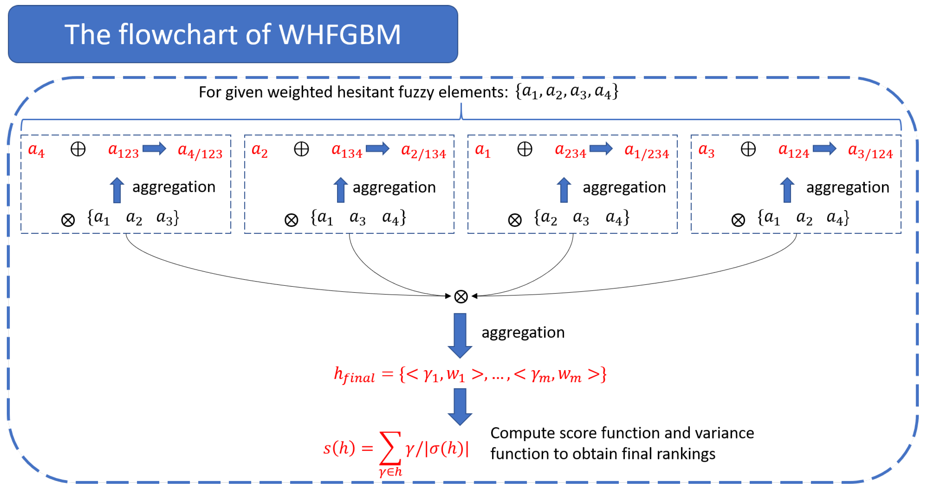
The flowchart and algorithm of the proposed operator, WHFGBM, are displayed in Figure 1 and Algorithm 1, respectively.

Algorithm 1 Weighted hesitant fuzzy geometric Bonferroni mean

Input: The collection of WHFEs $a_1,\dots a_n$, the constant $p,q$. Output: Aggregation result f.   1: Initialize relative parameters and WHFEs.   2: Construct empty set $All=\left\{\right\}$.   3: for $i\leftarrow 1$ to n do   4:    Construct empty set $Temp=\left\{\right\}$.   5:    for $j\leftarrow 1$ to n do   6:      if j is not equal to i then   7:         Compute ${\left(q{a}_j\right)}^{{\displaystyle \frac{1}{n-1}}}$ through $\lambda h^w$ and ${\left(h^w\right)}^{\lambda }$ operators and put into set $Temp$.   8:      end if   9:    end for 10:    Adopt ⊗ to aggregate WHFEs from $Temp$ to produce $a_T$. 11:    Adopt ⊕ to aggregate $p{a}_i$ and $a_T$, obtain result and put in $All$. 12: end for 13: Adopt ⊕ operator to aggregate all WHFEs from $All$ with the constant $p,q$. 14: Obtain final result f of fuzzy information fusion.

4. Numerical Example

In this section, a series of numerical examples is provided to compare the proposed method with existing methods.

Example 3.

To enhance the working efficiency, the university is considering purchasing a new information system. Assuming there are some software packages available, the managers from the university need to obtain the best plan after comprehensive consideration. After the initial selection, $A_1,A_2,A_3,A_4$ are the four candidates. Then, three experts, $E_k(k=1,2,3)$, will give their final scores from different views to decide which information system will be the best choice. In the whole decision-making process, three experts give their own preferences, respectively. The following four attributes will be the main factors taken into consideration:

• Capitalized costs for information system construction ($C_1$).
• Performance improvement for the whole organization ($C_2$).
• Migration costs and sunk costs ($C_3$).
• The reliability of software developer ($C_4$).

For different attributes ($C_j(j=1,2,3,4)$), these attributes have different weights $w={(0.3,0.25,0.25,0.2)}^T$. $A^{\left(k\right)}=\left(r_{ij}^{\left(k\right)}\right)(k=1,2,3)$ (seen in

Table 1. The preference matrix provided by $E_1$, $E_2$, and $E_3$.

	${\mathit{E}}_1$				${\mathit{E}}_2$				${\mathit{E}}_3$
	${\mathit{C}}_{\mathbf{1}}$	${\mathit{C}}_{\mathbf{2}}$	${\mathit{C}}_{\mathbf{3}}$	${\mathit{C}}_{\mathbf{4}}$	${\mathit{C}}_{\mathbf{1}}$	${\mathit{C}}_{\mathbf{2}}$	${\mathit{C}}_{\mathbf{3}}$	${\mathit{C}}_{\mathbf{4}}$	${\mathit{C}}_{\mathbf{1}}$	${\mathit{C}}_{\mathbf{2}}$	${\mathit{C}}_{\mathbf{3}}$	${\mathit{C}}_{\mathbf{4}}$
$A_1$	0.6	0.8	0.5	0.6	0.6	0.85	0.65	0.6	0.8	0.85	0.65	0.7
$A_2$	0.5	0.9	0.8	0.7	0.7	0.8	0.8	0.75	0.7	0.8	0.8	0.75
$A_3$	0.7	0.6	0.7	0.6	0.8	0.6	0.75	0.6	0.7	0.8	0.75	0.9
$A_4$	0.8	0.7	0.8	0.9	0.8	0.7	0.8	0.85	0.9	0.75	0.85	0.9

) is constructed, and $r_{ij}^{\left(k\right)}\in [0,1]$ represents the evaluation degree of every expert $E_k(k=1,2,3)$ to every alternative $A_i$ under attribute $C_j$. Through our proposed method, we provide solutions to this problem.

In comparison, two aggregation operators, WHFHA/WHFHG, are used to aggregate hesitant fuzzy information. To illustrate results, a comparison with WHFWA and WHFWG operators [37] is made. The definition of these operators is as follows:

$$WHFWA(h_1^w,\dots ,h_n^w)={\oplus }_{j=1}^n\left(w_j{h}_j^w\right)=\bigcup _{{\gamma }_1\in h_1^w,\dots ,{\gamma }_n\in h_n^w}\left\{<1-\prod _{j=1}^n{(1-{\gamma }_j)}^{w_j},w_{{\gamma }_1}\dots w_{{\gamma }_n}>\right\}$$

$$WHFWG(h_1^w,\dots ,h_n^w)={\otimes }_{j=1}^n{\left(h_j^w\right)}^{w_j}=\bigcup _{{\gamma }_1\in h_1^w,\dots ,{\gamma }_n\in h_n^w}\left\{<\prod _{j=1}^n{\gamma }_j^{w_j},w_{{\gamma }_1}{w}_{{\gamma }_2}\dots w_{{\gamma }_n}>\right\}$$

Case 5 In this case, assume that the weight of every expert is unknown, and evaluation results from decision makers are anonymous.

Step 1 Firstly, WHFSs $A=\{<r_{ij},w_{r_{ij}}>\}$ are obtained as follows:

For $A_1$

$h_{A_1}^w\left(C_1\right)=\{<0.6,{\displaystyle \frac{2}{3}}>,<0.8,{\displaystyle \frac{1}{3}}>\},h_{A_1}^w\left(C_2\right)=\{<0.8,{\displaystyle \frac{1}{3}}>,<0.85,{\displaystyle \frac{2}{3}}>\}$

$h_{A_1}^w\left(C_3\right)=\{<0.5,{\displaystyle \frac{1}{3}}>,<0.65,{\displaystyle \frac{2}{3}}>\},h_{A_1}^w\left(C_4\right)=\{<0.6,{\displaystyle \frac{2}{3}}>,<0.7,{\displaystyle \frac{1}{3}}>\}$

For $A_2$

$h_{A_2}^w\left(C_1\right)=\{<0.5,{\displaystyle \frac{1}{3}}>,<0.7,{\displaystyle \frac{2}{3}}>\},h_{A_2}^w\left(C_2\right)=\{<0.8,{\displaystyle \frac{2}{3}}>,<0.9,{\displaystyle \frac{1}{3}}>\}$

$h_{A_2}^w\left(C_3\right)=\{<0.8,1>\},h_{A_2}^w\left(C_4\right)=\{<0.7,{\displaystyle \frac{1}{3}}>,<0.75,{\displaystyle \frac{2}{3}}>\}$

For $A_3$

$h_{A_3}^w\left(C_1\right)=\{<0.7,{\displaystyle \frac{2}{3}}>,<0.8,{\displaystyle \frac{1}{3}}>\},h_{A_3}^w\left(C_2\right)=\{<0.6,{\displaystyle \frac{2}{3}}>,<0.8,{\displaystyle \frac{1}{3}}>\}$

$h_{A_3}^w\left(C_3\right)=\{<0.7,{\displaystyle \frac{1}{3}}>,<0.75,{\displaystyle \frac{2}{3}}>\},h_{A_3}^w\left(C_4\right)=\{<0.6,{\displaystyle \frac{2}{3}}>,<0.9,{\displaystyle \frac{1}{3}}>\}$

For $A_4$

$h_{A_4}^w\left(C_1\right)=\{<0.8,{\displaystyle \frac{2}{3}}>,<0.9,{\displaystyle \frac{1}{3}}>\},h_{A_4}^w\left(C_2\right)=\{<0.7,{\displaystyle \frac{2}{3}}>,<0.75,{\displaystyle \frac{1}{3}}>\}$

$h_{A_4}^w\left(C_3\right)=\{<0.8,{\displaystyle \frac{2}{3}}>,<0.85,{\displaystyle \frac{1}{3}}>\},h_{A_4}^w\left(C_4\right)=\{<0.85,{\displaystyle \frac{1}{3}}>,<0.9,{\displaystyle \frac{2}{3}}>\}$

Step 2 The WHFHA operator is applied to aggregate WHFEs of every sample. The results are displayed in

Table 2. The results of the WHFWA operator.

WHFS	The Results of the WHFWA Operator
$h_{A_1}^w$	$\{<0.8183,0.0123>\}$, $\{<0.8313,0.0247>\}$, $\{<0.8526,0.0247>\}$, $\{<0.8632,0.0494>\}$, $\{<0.8863,0.0247>\}$, $\{<0.8944,0.0494>\}$, $\{<0.9078,0.0494>\}$, $\{0.9123,0.0247\}$, $\{<0.9144,0.0988>\}$, $\{<0.9186,0.0494>\}$, $\{<0.9289,0.0494>\}$, $\{<0.934,0.0988>\}$, $\{<0.9451,0.0494>\}$, $\{<0.949,0.0988>\}$, $\{<0.9555,0.0988>\}$, $\{<0.9587,0.1975>\}$
$h_{A_2}^w$	$\{<0.9507,0.037>\}$, $\{<0.9637,0.0741>\}$, $\{<0.9708,0.0741>\}$, $\{<0.9722,0.0741>\}$, $\{<0.9785,0.1481>\}$, $\{<0.9795,0.1481>\}$, $\{<0.9835,0.1481>\}$, $\{<0.9878,0.2963>\}$
$h_{A_3}^w$	$\{<0.8757,0.0247>\}$, $\{<0.8846,0.0494>\}$, $\{<0.8937,0.0123>\}$, $\{<0.9014,0.0247>\}$, $\{<0.9048,0.0494>\}$, $\{<0.9116,0.0988>\}$, $\{<0.9186,0.0247>\}$, $\{<0.9244,0.0494>\}$, $\{<0.9263,0.0494>\}$, $\{<0.9316,0.0988>\}$, $\{<0.937,0.0247>\}$, $\{<0.9415,0.0494>\}$, $\{<0.9435,0.0988>\}$, $\{<0.9476,0.1975>\}$, $\{<0.9517,0.0494>\}$, $\{<0.9552,0.0988>\}$
$h_{A_4}^w$	$\{<0.9175,0.0123>\}$, $\{<0.9392,0.0247>\}$, $\{<0.9413,0.0247>\}$, $\{<0.9469,0.0247>\}$, $\{<0.9567,0.0494>\}$, $\{<0.9609,0.0494>\}$, $\{<0.9622,0.0494>\}$, $\{<0.9665,0.0247>\}$, $\{<0.9722,0.0988>\}$, $\{<0.9753,0.0494>\}$, $\{<0.9762,0.0494>\}$, $\{<0.9785,0.0494>\}$, $\{<0.9825,0.0988>\}$, $\{<0.9841,0.0988>\}$, $\{<0.9847,0.0988>\}$, $\{<0.9887,0.1975>\}$

.

Step 3 Through the equation above, the score and variance of $h^w\left(A_i\right)(i=1,2,3,4)$ are obtained:

$s\left(h^w\left(A_1\right)\right)=0.9256$, $v\left(h^w\left(A_1\right)\right)=0.0345$, $s\left(h^w\left(A_2\right)\right)=0.9790$, $v\left(h^w\left(A_2\right)\right)=0.0090$, $s\left(h^w\left(A_3\right)\right)=0.9307$, $v\left(h^w\left(A_3\right)\right)=0.0213$, $s\left(h^w\left(A_4\right)\right)=0.9747$, $v\left(h^w\left(A_4\right)\right)=0.0148$.

Step 4 To produce the final ranking results, these samples are ranked according to $s\left(h^w\left(A_i\right)\right)$. Therefore, the rankings of every sample: $A_2\succ A_4\succ A_3\succ A_1$ are obtained, and the best sample is $A_2$.

Step 2: The WHFWG operator is applied to aggregate WHFEs of every sample. The results of the WHFWG operator are displayed in

Table 3. The results of the WHFWG operator.

WHFS	The Results of the WHFWG Operator
$h_{A_1}^w$	$\{<0.3407,0.1975>\}$, $\{<0.3525,0.0988>\}$, $\{<0.3604,0.0988>\}$, $\{<0.3729,0.0494>\}$, $\{<0.4253,0.0988>\}$, $\{<0.44,0.0494>\}$, $\{<0.4447,0.0988>\}$, $\{<0.4499,0.0494>\}$, $\{<0.46,0.0494>\}$, $\{<0.4654,0.0247>\}$, $\{<0.4703,0.0494>\}$, $\{<0.4866,0.0247>\}$, $\{<0.555,0.0494>\}$, $\{<0.5742,0.0247>\}$, $\{<0.587,0.0247>\}$, $\{<0.6073,0.0123>\}$,
$h_{A_2}^w$	$\{<0.4487,0.2963>\}$, $\{<0.4517,0.1481>\}$, $\{<0.4826,0.1481>\}$, $\{<0.4859,0.0741>\}$, $\{<0.5027,0.1481>\}$, $\{<0.5061,0.0741>\}$, $\{<0.5407,0.0741>\}$, $\{<0.5443,0.037>\}$
$h_{A_3}^w$	$\{<0.3293,0.1975>\}$, $\{<0.3542,0.0988>\}$, $\{<0.3878,0.0988>\}$, $\{<0.4171,0.0494>\}$, $\{<0.4298,0.0988>\}$, $\{<0.447,0.0988>\}$, $\{<0.4623,0.0494>\}$, $\{<0.4808,0.0494>\}$, $\{<0.5061,0.0494>\}$, $\{<0.5263,0.0494>\}$, $\{<0.5443,0.0247>\}$, $\{<0.5661,0.0247>\}$, $\{<0.5833,0.0494>\}$, $\{<0.6274,0.0247>\}$, $\{<0.6868,0.0247>\}$, $\{<0.7388,0.0123>\}$,
$h_{A_4}^w$	$\{<0.5458,0.1975>\}$, $\{<0.5546,0.0988>\}$, $\{<0.5999,0.0988>\}$, $\{<0.6096,0.0494>\}$, $\{<0.6115,0.0988>\}$, $\{<0.6214,0.0494>\}$, $\{<0.629,0.0988>\}$, $\{<0.6392,0.0494>\}$, $\{<0.6721,0.0494>\}$, $\{<0.683,0.0247>\}$, $\{<0.6914,0.0494>\}$, $\{<0.7026,0.0247>\}$, $\{<0.7047,0.0494>\}$, $\{<0.7161,0.0247>\}$, $\{<0.7746,0.0247>\}$, $\{<0.7871,0.0123>\}$

.

Step 3: Through the equation above, the score and variance of the $h^w\left(A_i\right)$ of every sample are obtained. $s\left(h^w\left(A_1\right)\right)=0.4190$, $v\left(h^w\left(A_1\right)\right)=0.0724$, $s\left(h^w\left(A_2\right)\right)=0.4975$, $v\left(h^w\left(A_2\right)\right)=0.0312$, $s\left(h^w\left(A_3\right)\right)=0.4409$, $v\left(h^w\left(A_3\right)\right)=0.0964$, $s\left(h^w\left(A_4\right)\right)=0.6196$, $v\left(h^w\left(A_4\right)\right)=0.0613$.

Step 4: To produce the final ranking results, these samples are ranked according to $s\left(h^w\left(A_i\right)\right)$ and $v\left(h^w\left(A_i\right)\right)$. Therefore, the rankings of every sample ($A_4\succ A_2\succ A_3\succ A_1$) are obtained, and the best sample is $A_4$.

For this example, the proposed method—WHFGBM operator—is applied to aggregate these WHFEs. After computation, the novel rankings of these examples is obtained ($A_4\succ A_2\succ A_3\succ A_1$), and the best sample is $A_4$. It is easy to know that WHFGBM has the same ranking as WHFWG; these two operators provide the same best choice. However, WHFWA provides a divergent result, owing to the difference between $A_2$ and $A_4$.

Example 4

([37]). Site choice is a common multi-criteria decision-making problem a factory considers when adding new construction for production capacity expansion. Three attributes $G_i(i=1,2,3)$ are factors influencing the final decision, including

• $G_1$: Price;
• $G_2$: Location;
• $G_3$: Environment.

After the initial selection and experts’ evaluation, the decision-making matrix, including weighted hesitant fuzzy data, is obtained. WHFE can be represented by $h_{ij}^w={\bigcup }_{{\gamma }_{ij}\in h_{ij}^w}\{<{\gamma }_{ij},w_{{\gamma }_{ij}}>\}$, where $w_{{\gamma }_{ij}}$ and ${\gamma }_{ij}$ are weights and membership degree values, respectively, which describe the candidate $Y_i$ to the attribute $G_j$. These data, described by WHFEs, are displayed in

Table 4. Weighted hesitant fuzzy decision matrix.

	${\mathit{G}}_1$	${\mathit{G}}_2$	${\mathit{G}}_3$
$Y_1$	{(0.6,0.3),(0.5,0.3),(0.4,0.4)}	{(0.6,0.8),(0.4,0.2)}	{(0.5,0.3),(0.3,0.7)}
$Y_2$	{(0.4,0.6),(0.3,0.4)}	{(0.8,1)}	{(0.4,0.2),(0.3,0.3),(0.2,0.5)}
$Y_3$	{(0.8,1)}	{(0.7,0.1),(0.6,0.3),(0.5,0.6)}	{(0.2,0.5),(0.1,0.5)}

.

Remark 1.

The score and variance of $h^w\left(Y_i\right)$ of every sample are obtained. The results of WHFWA: $s\left(h^w\left(Y_1\right)\right)=0.6445$, $v\left(h^w\left(Y_1\right)\right)=0.1072$, $s\left(h^w\left(Y_2\right)\right)=0.8585$, $v\left(h^w\left(Y_2\right)\right)=0.0115$, $s\left(h^w\left(Y_3\right)\right)=0.8686$, $v\left(h^w\left(Y_3\right)\right)=0.0140$. The results of WHFWG: $s\left(h^w\left(Y_1\right)\right)=0.2962$, $v\left(h^w\left(Y_1\right)\right)=0.1037$, $s\left(h^w\left(Y_2\right)\right)=0.2844$, $v\left(h^w\left(Y_2\right)\right)=0.0762$, $s\left(h^w\left(Y_3\right)\right)=0.2289$, $v\left(h^w\left(Y_3\right)\right)=0.0528$. The rankings of WHFWA and WHFWG are: $Y_3\succ Y_2\succ Y_1$ and $Y_1\succ Y_2\succ Y_3$, respectively. The proposed operator WHFGBM is applied to obtain the final rankings: $Y_1\succ Y_3\succ Y_2$. WHFGBM gives the same best choice as WHFWG, but both of them have differences regarding $Y_2$ and $Y_3$. Even though this case has only three samples, WHFWA yields contradiction rankings with WHFWG.

Example 5.

To further validate the proposed operator, the hesitant fuzzy data from the paper [32] are utilized. Weights to transfer HFEs data to WHFEs data are added by fusing equal weights. All the data are shown in

Table 5. Weighted hesitant fuzzy decision matrix.

	${\mathit{G}}_1$	${\mathit{G}}_2$
$Y_1$	{(0.2,1/3),(0.4,1/3),(0.7,1/3)}	{(0.2,1/3),(0.6,1/3),(0.8,1/3)}
$Y_2$	{(0.2,1/4),(0.4,1/4),(0.7,1/4),(0.9,1/4)}	{(0.1,1/4),(0.2,1/4),(0.4,1/4),(0.5,1/4)}
$Y_3$	{(0.3,1/4),(0.5,1/4),(0.6,1/4),(0.7,1/4)}	{(0.2,1/4),(0.4,1/4),(0.5,1/4),(0.6,1/4)}
$Y_4$	{(0.3,1/3),(0.5,1/3),(0.6,1/3)}	{(0.2,1/2),(0.4,1/2))}
	${\mathit{G}}_{\mathbf{3}}$
$Y_1$	{(0.2,1/5),(0.3,1/5),(0.6,1/5),(0.7,1/5),(0.9,1/5)}
$Y_2$	{(0.3,1/4),(0.4,1/4),(0.6,1/4),(0.9,1/4)}
$Y_3$	{(0.3,1/4),(0.5,1/4),(0.7,1/4),(0.8,1/4)}
$Y_4$	{(0.5,1/3),(0.6,1/3),(0.7,1/3)}

.

Remark 2.

The score and variance of $h^w\left(Y_i\right)$ for each sample are obtained. The results of WHFWA: $s\left(h^w\left(Y_1\right)\right)=0.4950$, $v\left(h^w\left(Y_1\right)\right)=0.1375$, $s\left(h^w\left(Y_2\right)\right)=0.4390$, $v\left(h^w\left(Y_2\right)\right)=0.1488$, $s\left(h^w\left(Y_3\right)\right)=0.4367$, $v\left(h^w\left(Y_3\right)\right)=0.0880$, $s\left(h^w\left(Y_4\right)\right)=0.5067$, $v\left(h^w\left(Y_4\right)\right)=0.0624$. The results of WHFWG: $s\left(h^w\left(Y_1\right)\right)=0.5003$, $v\left(h^w\left(Y_1\right)\right)=0.1384$, $s\left(h^w\left(Y_2\right)\right)=0.5091$, $v\left(h^w\left(Y_2\right)\right)=0.1189$, $s\left(h^w\left(Y_3\right)\right)=0.5782$, $v\left(h^w\left(Y_3\right)\right)=0.0907$, $s\left(h^w\left(Y_4\right)\right)=0.3493$, $v\left(h^w\left(Y_4\right)\right)=0.0707$. The rankings of WHFWA and WHFWG are $Y_4\succ Y_1\succ Y_3\succ Y_2$ and $Y_3\succ Y_2\succ Y_1\succ Y_4$, respectively. The proposed operator WHFGBM is applied to obtain the final rankings of samples: $Y_3\succ Y_1\succ Y_2\succ Y_4$. WHFGBM gives the same best choice as WHFWG. These two operators have a slight difference between $Y_1$ and $Y_2$ samples. However, WHFWA provides an almost contradiction best choice.

Example 6.

To compare different methods, data from the paper [39] are adopted. Assume the ideal solution is $A^{\ast }=\left\{1\right\}$, and aggregation operator and score function are used for obtaining results. Related decision-making data, as shown in

Table 6. Weighted hesitant fuzzy decision matrix.

	${\mathit{P}}_1$	${\mathit{P}}_2$
$A_1$	{(0.5,1/3),(0.4,1/3),(0.3,1/3)}	{(0.9,1/4),(0.8,1/4),(0.7,1/4),(0.1,1/4)}
$A_2$	{(0.5,1/2),(0.3,1/2)}	{(0.9,1/4),(0.7,1/4),(0.6,1/4),(0.2,1/4)}
$A_3$	{(0.7,1/2),(0.6,1/2)}	{(0.9,1/2),(0.6,1/2)}
$A_4$	{(0.8,1/4),(0.7,1/4),(0.4,1/4),(0.3,1/4)}	{(0.7,1/3),(0.4,1/3),(0.2,1/3)}
$A_5$	{(0.9,1/5),(0.7,1/5),(0.6,1/5),(0.3,1/5),(0.1,1/5)}	{(0.8,1/4),(0.7,1/4),(0.6,1/4),(0.4,1/4)}
	${\mathit{P}}_{\mathbf{3}}$
$A_1$	{(0.5,1/3),(0.4,1/3),(0.2,1/3)}
$A_2$	{(0.8,1/4),(0.6,1/4),(0.5,1/4),(0.1,1/4)}
$A_3$	{(0.7,1/3),(0.5,1/3),(0.3,1/3)}
$A_4$	{(0.8,1/2),(0.1,1/2)}
$A_5$	{(0.9,1/3),(0.8,1/3),(0.7,1/3)}

, are collected to form weighted hesitant fuzzy sets.

Remark 3.

Score and variance of $h^w\left(A_i\right)$ for each sample are obtained. The results of WHFWA: $s\left(h^w\left(A_1\right)\right)=0.4700$, $v\left(h^w\left(A_1\right)\right)=0.1170$, $s\left(h^w\left(A_2\right)\right)=0.4841$, $v\left(h^w\left(A_2\right)\right)=0.1067$, $s\left(h^w\left(A_3\right)\right)=0.7806$, $v\left(h^w\left(A_3\right)\right)=0.0795$, $s\left(h^w\left(A_4\right)\right)=0.5451$, $v\left(h^w\left(A_4\right)\right)=0.1859$. $s\left(h^w\left(A_5\right)\right)=0.6326$, $v\left(h^w\left(A_5\right)\right)=0.0854$. The results of WHFWG: $s\left(h^w\left(A_1\right)\right)=0.4391$, $v\left(h^w\left(A_1\right)\right)=0.1075$, $s\left(h^w\left(A_2\right)\right)=0.4466$, $v\left(h^w\left(A_2\right)\right)=0.1090$, $s\left(h^w\left(A_3\right)\right)=0.5440$, $v\left(h^w\left(A_3\right)\right)=0.0858$, $s\left(h^w\left(A_4\right)\right)=0.3785$, $v\left(h^w\left(A_4\right)\right)=0.1986$. $s\left(h^w\left(A_5\right)\right)=0.6934$, $v\left(h^w\left(A_5\right)\right)=0.1142$. The rankings of WHFWA and WHFWG are $A_3\succ A_5\succ A_4\succ A_2\succ A_1$ and $A_5\succ A_3\succ A_2\succ A_1\succ A_4$, respectively. Generalized hybrid hesitant weighted distance is proposed by [39]; when $\lambda =1$, the ranking is $A_3\succ A_5\succ A_4\succ A_1\succ A_2$. The proposed operator WHFGBM is applied to obtain the final rankings of samples: $A_5\succ A_3\succ A_2\succ A_1\succ A_4$. This case includes the most samples compared with other cases. Experts give different judgments based on attributes $P_1,P_2,P_3$. Experts give a concentrated judgment for $A_3$, which can be seen from WHFEs with short length. WHFWA and generalized hybrid hesitant weighted distance give an almost consistent ranking, only having a slight difference in inferior samples. WHFWG and WHFGBM provide consistent rankings.

Parameter selection: For the WHFGBM operator, there exist two parameters, p and q. When these two parameters are assigned, the WHFGBM operator will finalize. When the decision-making process begins, the WHFEs, as input data, will be sent to the WHFGBM to complete aggregation. Typically, the parameters p and q are small values, which makes the values of the final results to be in a reasonable range for comparison. For above numeric examples, the two parameters values, $p=1$ and $q=2$, are assigned, respectively. If the values of parameters become bigger, the power operator and ⊗ operator will make the values become very small, which is not conducive to comparison. Hence, these two parameters are usually 1 or 2.

Parameter sensitivity: Due to the influence of parameter values, the sensitivity of the proposed operator should be considered. From the above analysis, the values of two parameters should be greater than 0 but not too large. Values of $p=1$ and $q=2$ are assigned for the above numeric examples. Combinations of $p=1,q=1$, $p=2,q=1$, and $p=2,q=2$ are assigned for further analysis. For example 3, the same ranking results are obtained: $A_4\succ A_2\succ A_1\succ A_3$. For example 4, when $p=1,q=1$, $p=2,q=2$, and $p=2,q=1$, the results are $Y_3\succ Y_1\succ Y_2$, which are slightly different from those when $p=1,q=2$. For example 5, when $p=1,q=1$, the same results are obtained: $Y_3\succ Y_2\succ Y_1\succ Y_4$. When $p=2,q=2$ and $p=2,q=1$, the results are slightly different: $Y_3\succ Y_1\succ Y_2\succ Y_4$. For example 6, the same results are obtained: $A_5\succ A_3\succ A_2\succ A_1\succ A_4$. From the above results, in example 3 and example 6, any $p,q$ combination can provide the same results. In example 5, one combination provides slightly different results from the other three combinations. In example 4, results from different combinations are slightly different. Hence, the proposed operator can provide stable results, and it has robustness for decision-making tasks.

5. Conclusions

Weighted hesitant fuzzy theory allows every membership degree to have positive value weights to further depict fuzzy information. In this paper, some operations (“⊕” and “⊗” operations of WHFEs) are redefined intuitively and logically, and properties and corresponding proofs are given. Further, the WHFWA and WHFWG aggregation operators are introduced to develop a novel WHFGBM operator. The novel operator will integrate fuzzy information better in multi-criteria decision-making problems. Finally, the results of numeric examples are displayed to validate the effectiveness and feasibility of the proposed operator. Although our operator can provide an aggregation method based on WHFS, when attributes increase, the computation burden will become heavier, which is the main limitation for subsequent large-scale expansion.

In the future, we will be dedicated to developing novel aggregation operators based on WHFSs and applying them to multi-criteria group decision-making problems, enhancing the information fusion ability under different scenarios. We will propose more types of mean operators, such as extending the operator to interval-valued WHFS. Then, we will consider introducing these operators to broader fuzzy decision-making fields, practical and complex scenarios. Further, we hope that our research will inspire more efficient tools for MCDM. On the other hand, introducing the advantages of existing operators is considered to improve the robustness of the operator. In addition, the weights for WHFS are important. However, the most common way to obtain weights is by experience, which increases the uncertainty. Hence, obtaining attributes objectively is definitely one of the directions for future research.

References

1. Zadeh, L.A. Fuzzy sets. Inf. Control 1965, 8, 338–353. [Google Scholar] [CrossRef] [Scilit]
2. Atanassov, K.; Stoeva, S. Intuitionistic fuzzy sets. Fuzzy Sets Syst. 1986, 31, 343–349. [Google Scholar] [CrossRef] [Scilit]
3. Yager, R.R. Pythagorean fuzzy subsets. In Proceedings of the IFSA World Congress & Nafips Meeting, Edmonton, AB, Canada, 24–28 June 2013. [Google Scholar]
4. Zadeh, L.A. The concept of a linguistic variable and its application to approximate reasonin–I. Inf. Sci. 1975, 8, 199–249. [Google Scholar] [CrossRef] [Scilit]
5. Zadeh, L.A. The concept of a linguistic variable and its application to approximate reasoning–II. Inf. Sci. 1975, 8, 301–357. [Google Scholar] [CrossRef] [Scilit]
6. Zadeh, L.A. The concept of a linguistic variable and its application to approximate reasoning–III. Inf. Sci. 1975, 9, 43–80. [Google Scholar] [CrossRef] [Scilit]
7. Dubois, D.; Prade, H. Fuzzy Sets and Systems: Theory and Applications; Academic Press: Cambridge, MA, USA, 1980. [Google Scholar]
8. Torra, V. Hesitant fuzzy sets. Int. J. Intell. Syst. 2010, 25, 529–539. [Google Scholar] [CrossRef] [Scilit]
9. Torra, V.; Yasuo, N. On hesitant fuzzy sets and decision. In Proceedings of the 2009 IEEE International Conference on Fuzzy Systems, Jeju, Republic of Korea, 20–24 August 2009. [Google Scholar]
10. Wang, P.Z.; Zhu, B.Y.; Yan, K.Y.; Zhang, Z.Y.; Ali, Z.; Pamucar, D. Power aggregation operators based on Aczel-Alsina T-norm and T-conorm for intuitionistic hesitant fuzzy information and their application to logistics service provider selection. Artifical Intell. Rev. 2022, 58, 204. [Google Scholar] [CrossRef] [Scilit]
11. Uluay, V.; Deli, I.; Edalatpanah, S. Prioritized Aggregation Operators of GTHFNs MADM Approach for the Evaluation of Renewable Energy Sources. Informatica 2024, 35, 859–882. [Google Scholar] [CrossRef] [Scilit]
12. Kavitha, S.; Janani, K.; Mohanrasu, S.; Satheeshkumar, J.; Amudha, T.; Rakkiyappan, R. Ensemble feature selection using q-rung orthopair hesitant fuzzy Hamacher, Einstein and Dombi Aggregation operators. Appl. Soft Comput. 2024, 161, 111752. [Google Scholar] [CrossRef] [Scilit]
13. Shit, C.; Ghorai, G. A novel Aczel-Alsina aggregation operators based multi-criteria group decision making approach under Hesitant fuzzy set for the selection of best brand in Educational Institution. Eng. Appl. Artif. Intell. 2025, 158, 111464. [Google Scholar] [CrossRef] [Scilit]
14. Sun, Z.; Ali, Z.; Mahmood, T.; Liu, P. Complex Pythagorean Hesitant Fuzzy Aggregation Operators Based on Aczel-Alsina t-Norm and t-Conorm and Their Applications in Decision-Making. Int. J. Fuzzy Syst. 2024, 26, 1091–1106. [Google Scholar] [CrossRef] [Scilit]
15. Özlü, C. Bipolar-Valued Complex Hesitant fuzzy Dombi Aggregating Operators Based on Multi-criteria Decision-Making Problems. Int. J. Fuzzy Syst. 2025, 27, 2199–3211. [Google Scholar] [CrossRef] [Scilit]
16. Dong, J.Y.; Gong, S.H.; Wan, S.P. Probabilistic linguistic hesitant fuzzy multi-attribute decision making for rural revitalization project selection of China. Appl. Intell. 2025, 55, 1573–7497. [Google Scholar] [CrossRef] [Scilit]
17. Muhammad, Q.; Muhammad, N.; Zahid, K.; Samuel, O. Interval-Valued Probabilistic Dual Hesitant Fuzzy Muirhead Mean Aggregation Operators and Their Applications in Regenerative Energy Source Selection. Int. J. Intell. Syst. 2025, 2025, 8892299. [Google Scholar]
18. Gupta, P.; Hait, S.R.; Raval, V.; Mandal, S.; Guha, D.; Chakraborty, D. Bonferroni Mean Pre-aggregation Operator Assisted Dynamic Fuzzy Histogram Equalization for Retinal Vascular Segmentation. IEEE J. Biomed. Health Inform. 2026, 30, 425–435. [Google Scholar] [CrossRef] [Scilit]
19. Maneckshaw, B.; Mahapatra, G.; Barker, K. Multi-objective redundancy allocation integrating interval uncertainty and hesitant fuzzy aggregation with a non-dominated sorting genetic algorithm. Expert Syst. Appl. 2026, 299, 129956. [Google Scholar] [CrossRef] [Scilit]
20. Mahmood, T.; Waqas, H.M.; Rehman, U. Selection of optimal encryption algorithm based on hesitant bipolar complex fuzzy frank aggregation operators. J. Appl. Math. Comput. 2024, 71, 1361–1395. [Google Scholar] [CrossRef] [Scilit]
21. Jiang, J.; Liu, X.D.; Wang, Z.; Ding, W.; Zhang, S.; Xu, H. Large group decision-making with a rough integrated asymmetric cloud model under multi-granularity linguistic environment. Inf. Sci. 2024, 678, 120994. [Google Scholar] [CrossRef] [Scilit]
22. Hu, X.M.; Yang, S.X.; Zhu, Y.R. Multiple Attribute Decision-Making Based on Three-Parameter Generalized Weighted Heronian Mean. Mathematics 2021, 9, 1363. [Google Scholar] [CrossRef] [Scilit]
23. Yager, R.R. On generalized Bonferroni mean operators for multi-criteria aggregation. Int. J. Approx. Reason. 2009, 50, 1279–1286. [Google Scholar] [CrossRef] [Scilit]
24. Wei, G.W.; Zhao, X.F.; Lin, R.; Wang, H.J. Uncertain linguistic Bonferroni mean operators and their application to multiple attribute decision making. Appl. Math. Model. 2013, 37, 5277–5285. [Google Scholar] [CrossRef] [Scilit]
25. Xu, Z.S.; Chen, X.Q. A multi-criteria decision making procedure based on interval-valued intuitionistic fuzzy bonferroni means. J. Syst. Sci. Syst. Eng. 2011, 20, 217–228. [Google Scholar] [CrossRef] [Scilit]
26. Xia, M.M.; Xu, Z.S.; Zhu, B. Geometric Bonferroni means with their application in multi-criteria decision making. Knowl.-Based Syst. 2013, 40, 88–100. [Google Scholar] [CrossRef] [Scilit]
27. Beliakov, G.; James, S.; Mordelova, J.; Rueckschlossova, T.; Yager, R.R. Generalized Bonferroni mean operators in multi-criteria aggregation. Fuzzy Sets Syst. 2010, 161, 2227–2242. [Google Scholar] [CrossRef] [Scilit]
28. Liu, L.T.; Wu, X.X.; Chen, G.R. Picture Fuzzy Interactional Bonferroni Mean Operators via Strict Triangular Norms and Applications to Multicriteria Decision Making. IEEE Trans. Fuzzy Syst. 2023, 31, 2632–2644. [Google Scholar] [CrossRef] [Scilit]
29. Debnath, K.; Roy, S.K.; Deveci, M.; Tomáková, H. Integrated MADM approach based on extended MABAC method with Aczel-Alsina generalized weighted Bonferroni mean operator. Artif. Intell. Rev. 2025, 58, 27. [Google Scholar] [CrossRef] [Scilit]
30. Gowtham, R.N.; Hait, S.R.; Mahadevappa, G.M. Classification of epileptic EEG signals with the utilization of Bonferroni mean based fuzzy pattern tree. Expert Syst. Appl. 2024, 239, 122424. [Google Scholar]
31. Vommi, A.M.; Battula, T.K. A hybrid filter-wrapper feature selection using Fuzzy KNN based on Bonferroni mean for medical datasets classification: A COVID-19 case study. Expert Syst. Appl. 2023, 218, 119612. [Google Scholar] [CrossRef] [Scilit]
32. Xia, M.; Xu, Z. Hesitant fuzzy information aggregation in decision making. Int. J. Approx. Reason. 2011, 52, 395–407. [Google Scholar] [CrossRef] [Scilit]
33. Liao, H.C.; Xu, Z.S.; Xia, M.M. Multiplicative Consistency of Heistant Fuzzy Preference Relation and its Application in Group Decision Making. Int. J. Inf. Technol. Decis. Mak. 2014, 13, 47–76. [Google Scholar] [CrossRef] [Scilit]
34. Farhadinia, B. A Novel Method of Ranking Hesitant Fuzzy Values for Multiple Attribute Decision-Making Problems. Int. J. Intell. Syst. 2013, 28, 752–767. [Google Scholar] [CrossRef] [Scilit]
35. Rodríguez, R.M.; Martínez, L.; Torra, V.; Xu, Z.S.; Herrera, F. Hesitant Fuzzy Sets: State of the Art and Future Directions. Int. J. Intell. Syst. 2014, 29, 495–524. [Google Scholar] [CrossRef] [Scilit]
36. Li, D.Q.; Zeng, W.Y.; Li, J.H. Geometric Bonferroni Mean Operators. Int. J. Intell. Syst. 2016, 31, 1181–1197. [Google Scholar] [CrossRef] [Scilit]
37. Zhang, Z.M.; Wu, C. Weighted Hesitant Fuzzy Sets and Their Application to Multi-Criteria Decision Making. Br. J. Math. Comput. Sci. 2014, 4, 1091–1123. [Google Scholar] [CrossRef] [Scilit]
38. Zeng, W.; Ma, R.; Li, D.; Yin, Q.; Xu, Z.; Khalil, A.M. Novel operations of weighted hesitant fuzzy sets and their group decision making application. AIMS Math. 2022, 7, 14117–14138. [Google Scholar] [CrossRef] [Scilit]
39. Xu, Z.S.; Xia, M.M. Distance and similarity measures for hesitant fuzzy sets. Inf. Sci. 2011, 181, 2128–2138. [Google Scholar] [CrossRef] [Scilit]
Figure 1. The flowchart of the proposed operator WHFGBM.
Symmetry 18 00414 g001