A Multi-Strategy Augmented Newton–Raphson-Based Optimizer for Global Optimization Problems and Robot Path Planning

Abstract

Newton–Raphson-Based Optimizer (NRBO) is a recently proposed metaheuristic that combines mathematical search rules with population-based optimization; however, it still suffers from an insufficient balance between global exploration and local exploitation, limited local refinement accuracy, and weak adaptability in complex optimization scenarios. To address these limitations, this paper proposes an Improved Newton–Raphson-Based Optimizer (INRBO), which enhances the original framework through a multi-strategy augmentation mechanism. Specifically, INRBO integrates three complementary strategies: (1) an adaptive differential operator with a linearly decaying scaling factor to dynamically regulate exploration and exploitation throughout the search process; (2) a quadratic interpolation strategy that exploits high-quality individuals to improve local search directionality and precision; and (3) an elitist population genetic strategy that preserves superior solution characteristics while maintaining population diversity and preventing premature convergence. The performance of INRBO is systematically evaluated on the CEC2017 benchmark suite under multiple dimensions and compared with several state-of-the-art metaheuristic algorithms. Experimental results demonstrate that INRBO achieves superior optimization accuracy, convergence efficiency, and robustness across unimodal, multimodal, hybrid, and composite functions, which is further confirmed by statistical significance tests. In addition, INRBO is applied to mobile robot path planning in grid-based environments of different scales, where it consistently generates shorter, smoother, and safer paths than competing algorithms. Overall, the proposed INRBO provides an effective and robust optimization framework for global continuous optimization problems and real-world engineering applications, demonstrating both strong theoretical value and practical applicability.

1. Introduction

With the rapid development of industrial automation, emergency response operations, and intelligent service systems, the demand for autonomous navigation of mobile robots in complex environments has grown significantly. As the core component of robot navigation, path planning directly determines operational safety, motion efficiency, and energy consumption. In industrial workshops, robots must compute collision-free paths among densely arranged equipment and moving personnel [1]. In urban emergency rescue scenarios, such as fire sites or earthquake debris, robots must avoid high-temperature zones, hazardous obstacles, and toxic areas to quickly reach target locations for detection or rescue tasks [2]. In warehousing and logistics, AGV robots must perform efficient path optimization among large numbers of shelves and transportation aisles to improve material turnover efficiency [3]. Despite differences in operating conditions, these real-world applications share the same core requirements for path planning: the ability to generate optimal trajectories that minimize travel distance and energy consumption while maximizing safety margins in environments containing unknown or dynamic obstacles. At the same time, the planning system must exhibit robust adaptability and real-time responsiveness to environmental changes.

Traditional path planning methods such as A* and Dijkstra demonstrate practical effectiveness in static and relatively simple environments; however, they rely heavily on accurate environmental modeling. When applied to high-dimensional spaces with multiple obstacles or dynamically changing scenarios, these methods often encounter low search efficiency, susceptibility to local optima, and path redundancy issues [4,5]. For example, in large grid maps, the heuristic-driven search of the A* algorithm may produce excessively circuitous routes when obstacle density increases [5]. Although Dijkstra can theoretically guarantee a globally optimal solution, it must traverse all nodes in the state space, leading to exponential growth in computational complexity in large environments, making real-time planning difficult to achieve [6]. As robot applications continue to evolve toward high dynamism, high complexity, and high uncertainty, the limitations of traditional approaches become increasingly significant, highlighting the need for planning strategies with strong global search capability, robustness, and adaptability.

Intelligent optimization algorithms have emerged as an important direction for solving robot path planning problems in complex environments due to their independence from precise mathematical modeling, strong global optimization capability, and high robustness [7]. By simulating biological population behaviors, physical processes, or mathematical optimization mechanisms, these algorithms efficiently search for optimal trajectories within the solution space without relying on detailed prior environmental models. Moreover, through appropriate parameter control, they can effectively balance the contradiction between exploration (identifying promising new search regions) and exploitation (refining high-quality known solutions), thereby adapting to planning tasks with varying levels of environmental complexity.

Among intelligent optimization methods, swarm intelligence algorithms have become a major research branch due to their simple structure, ease of implementation, and strong scalability, and they have been widely applied in robot path planning. Since Kennedy et al. proposed the Particle Swarm Optimization (PSO) algorithm [8], numerous swarm intelligence algorithms have been developed and employed in trajectory planning tasks. For example, Fu et al. proposed the Secretary Bird Optimization Algorithm (SBOA), inspired by the survival strategies of secretary birds in natural environments, and applied it to 3D UAV path planning [9]. Shengwei Fu et al. further introduced the Red-Billed Blue Magpie Optimizer (RBMO) to address the slow convergence, low accuracy, and weak robustness of UAV path planning in 2D/3D environments and engineering applications [10]. Mohammad Hussein Amiri et al. designed the Hippo Optimization (HO) algorithm inspired by intrinsic behavioral patterns observed in hippopotamuses [11]. Xinpeng Xu proposed the Crocodile Ambush Optimization Algorithm (CAOA), a novel metaheuristic model inspired by crocodile energy-saving and ambush hunting behaviors. CAOA integrates adaptive energy decay modeling, random leader selection, and threshold-based solution reinitialization to balance exploration and exploitation throughout the search process [12]. Tian-Lei Wang et al. developed the Cuckoo Catfish Optimizer (CCO), which simulates the searching, predation, and parasitic behaviors exhibited by cuckoo catfish. The early iterations of CCO emphasize multi-dimensional envelope search and compressed space strategies, supplemented by auxiliary search operations that limit the escape boundaries of candidate solutions [13]. Dler O. Hasan et al. proposed the Griffon Vulture Optimization Algorithm (GVOA), inspired by coordinated foraging behaviors of griffon vulture flocks. GVOA integrates four core mechanisms—following, collective hunting, solitary searching, and carcass reconnaissance—to maintain a strong balance between exploration and exploitation [14]. In addition, Salah Kamel et al. introduced the Supercell Thunderstorm Algorithm (STA), inspired by meteorological strategies such as spiral airflow, tornado formation, and jet stream dynamics. STA is designed to simulate the formation and evolution of supercell thunderstorms and serves as a computational model for complex optimization processes [15].

In addition, to address the problems of slow convergence and suboptimal solutions encountered by baseline algorithms in path planning, many researchers have proposed improved metaheuristic methods. For example, to overcome the tendency of the Ant Colony Optimization (ACO) algorithm to fall into local optima, generate excessive turning points, and converge slowly in mobile robot path planning, Tianfeng Zhou et al. introduced an improved ACO method featuring an adaptive pheromone fluctuation operator and an uneven pheromone initialization strategy [16]. Tao Qiuyun et al. proposed an improved Particle Swarm Optimization (IPSO) approach for obtaining optimal AGV navigation routes [17]. Ran Zhang et al. integrated the Cauchy mutation operator, adaptive weights, and sine–cosine learning strategies into Harris Hawks Optimization (HHO) and developed an enhanced HHO-based algorithm capable of achieving better performance in complex 3D flight scenarios for UAV path planning [18]. Lun Zhu et al. embedded two Differential Evolution strategies into COA and proposed the Self-Adaptive DE–Coati Optimization Algorithm (SDECOA) for multi-robot cooperative path planning tasks [19]. Yaonan Dai et al. employed adaptive mechanisms and artificial potential field functions to develop a New Whale Optimization Algorithm (NWOA) for solving mobile robot navigation tasks with improved path quality and stability [20]. Zhengzong Wang et al. proposed a Multi-Strategy Enhanced Zebra Optimization Algorithm (MZOA) to overcome the limitations of the baseline Zebra Optimization Algorithm, such as premature convergence and weak global exploration ability, and demonstrated its effectiveness in robot path planning problems [21]. To address the challenges of low search efficiency, limited obstacle avoidance capability, and local stagnation in large-scale environments with dense irregular obstacles, Yuchao Wang et al. introduced a hybrid scheme combining an improved Golden Jackal Optimization (MGJO) algorithm with an Improved Dynamic Window Approach (IDWA) [22]. Xinhao Zhang et al. proposed a Hybrid Dung Beetle Optimization (HDBO) algorithm to enhance computation efficiency and trajectory quality of bio-inspired planning methods applied to greenhouse environments using 2D LiDAR mappings, based on improvements to the traditional DBO framework [23].

However, existing swarm intelligence algorithms still exhibit notable limitations when applied to complex path planning tasks. First, the balance between exploration and exploitation is often unstable. Many algorithms rely on fixed search mechanisms—for example, PSO requires manually tuned inertia weights and acceleration coefficients, which may lead to premature convergence due to excessive local exploitation in the early stages, or wasted computation caused by excessive global exploration in later iterations [24]. Second, their adaptability in high-dimensional environments remains insufficient. As grid resolution increases or environmental dimensionality rises, the search space expands rapidly, causing “dimension explosion,” which results in degraded optimization accuracy and slower convergence speed [25,26]. These shortcomings restrict the engineering applicability of swarm intelligence algorithms in real-world scenarios. Therefore, it is necessary to develop new intelligent optimization methods with dynamic search adaptability, strong robustness in high-dimensional problems, and more effective utilization of high-quality solution information.

The Newton–Raphson-Based Optimization (NRBO) algorithm, a recently proposed intelligent optimization method, integrates the Newton–Raphson Search Rule (NRSR) and a Trap Avoidance Operator (TAO), demonstrating certain advantages in continuous numerical optimization tasks. NRSR leverages the second-order Taylor expansion characteristics of the classical Newton–Raphson method, guiding individuals toward candidate optima based on gradient information. The TAO enhances global exploration ability by combining the current solution with the global best solution, improving the algorithm’s capability to escape local minima [27]. Compared with algorithms purely inspired by biological behavior, NRBO’s mathematically driven mechanism offers stronger directionality and stability during the search process, providing a promising technical foundation for complex path planning problems.

However, NRBO still exhibits several performance limitations when applied to practical path planning. First, its search mechanism lacks adaptive capabilities: fixed step sizes and control parameters are used throughout the exploration and convergence phases. This often causes insufficient global search in early iterations and increases the risk of premature convergence in high-dimensional grid environments. Second, the individual updating process relies heavily on random perturbation and fails to adequately exploit information from high-quality solutions, making it difficult for the algorithm to improve trajectory precision in later stages. As a result, redundant turning behaviors or insufficient safety margins may be generated along the planned paths. Furthermore, the absence of an effective mechanism to preserve and inherit elite solution characteristics slows down population evolution and weakens convergence efficiency [25,28]. These limitations make it challenging for NRBO to meet the demands of large-scale or obstacle-dense environments, indicating the need for strategic improvements to overcome performance bottlenecks and enhance its applicability in real-world path planning scenarios.

To address the core limitations of existing swarm intelligence algorithms in complex robotic path planning—namely the imbalance between exploration and exploitation, weak adaptability in high-dimensional environments, and insufficient utilization of high-quality solution information—this paper proposes an Improved Newton–Raphson-Based Optimization algorithm (INRBO), built upon NRBO and validated through numerical experiments and engineering applications. The main contributions are as follows:

(1)

Innovative algorithmic design of INRBO: To overcome NRBO’s performance bottlenecks, INRBO integrates three enhanced strategies to construct an efficient optimization framework. First, an adaptive differential operator strategy is introduced, where a linearly decaying scaling factor (from 0.5 to 0.2) is combined with mutation–crossover–selection operations guided by the global best solution. This enables large-step global exploration in early iterations and fine-tuned local exploitation later. Second, a quadratic interpolation strategy uses the fitness information of the current solution, a randomly selected elite solution, and the global best to formulate a quadratic predictive function, enabling directional estimation of promising search regions and improving local accuracy and information exploitation. Third, an elite population inheritance strategy constructs an elite pool (top three individuals per iteration), and applies linear crossover and Gaussian mutation to ensure stable inheritance of high-quality solution features while maintaining diversity and mitigating premature convergence.

(2)

Numerical performance evaluation of INRBO: Using the CEC2017 benchmark suite at dimensions 30, 50, and 100, INRBO is compared with nine state-of-the-art algorithms. Performance is assessed using metrics including mean fitness, standard deviation, and convergence characteristics to evaluate optimization accuracy and robustness across different function categories. Additionally, a Friedman non-parametric test is conducted to statistically validate the significance of INRBO’s performance improvements over competing methods.

(3)

Application of INRBO to robotic path planning: A grid-map modeling approach is adopted to construct 20 × 20, 40 × 40, and 60 × 60 environments, transforming the path planning task into a numerical optimization problem that minimizes path length while satisfying collision-avoidance constraints. Through comparative simulation experiments, INRBO is evaluated against other algorithms in terms of path length, smoothness, obstacle clearance, and convergence efficiency, demonstrating its strong practical capability in complex scenarios of varying scales.

The remainder of this paper is organized as follows: Section 2 presents the core principles of NRBO and systematically introduces the design concepts, mathematical formulations, and implementation procedures of the three enhancement strategies in INRBO. Section 3 conducts numerical experiments and performance analyses of INRBO, comparing its optimization accuracy, convergence speed, and robustness against nine state-of-the-art algorithms. Section 4 focuses on the application of INRBO to mobile robot path planning in various environments. Finally, Section 5 summarizes the key advantages of INRBO in numerical optimization and robotic path planning, highlights existing limitations, and outlines future research directions, including real-time replanning in dynamic environments, cooperative multi-robot path optimization, and lightweight algorithm deployment, providing guidance for subsequent studies.

2. Newton–Raphson-Based Optimizer and the Proposed INRBO

2.1. Newton–Raphson-Based Optimizer (NRBO)

NRBO innovatively integrates two core components: the Newton–Raphson Search Rule (NRSR) and the Trap Avoidance Operator (TAO). This integration endows the algorithm with unique optimization capabilities and solution advantages, demonstrating strong potential for tackling complex problems [27]. It should be noted that the Newton–Raphson method used in this paper is not the classic Newton–Raphson algorithm based on gradients and Hessian matrix inversion, but rather an approximate search mechanism inspired by the Newton–Raphson concept. This method heuristically estimates the search direction, eliminating the need for explicit gradient calculations or matrix inversions during implementation, thus effectively reducing computational complexity and making it more suitable for high-dimensional, nonlinear, and black-box optimization problems. To improve the clarity of mathematical expressions, this paper adopts the following unified conventions for symbols: vectors are represented by bold lowercase letters, matrices are represented by bold uppercase letters, and scalar or vector elements are represented by ordinary lowercase letters. Unless otherwise specified, all vectors are dim-dimensional column vectors.

2.1.1. Initialization

Similarly to other metaheuristic algorithms, NRBO initiates the search for the global optimum by generating an initial population of random particles within the bounds of the decision variables. Based on the population size, each individual is represented by a decision vector. The random initialization of the population is expressed as:

$${\mathit{x}}_{\mathit{i}}=lb+{rand}_i\times \left(ub-lb\right),i=\mathrm{1,2},\cdots ,Np$$

(1)

where $x_i$ denotes the position of the $i^{th}$ individual, and $rand$ is a uniformly distributed random number in the range (0,1), and it is an i.i.d. (independent and identically distributed) variable, it is generated independently for different dimensions and individuals.

2.1.2. Newton–Raphson Search Rule (NRSR)

The NRSR is a search strategy based on the classical Newton–Raphson Method (NRM). To derive NRSR, the function values $f(x-\epsilon )$ and $f(x+\epsilon )$ are expanded using Taylor series around $(x-\epsilon )$ and $(x+\epsilon )$ retaining second-order terms while ignoring higher-order terms. The first and second derivatives of $f\left(x\right)$ [27,29]:

$${\displaystyle \genfrac{}{}{0pt}{}{f^{\prime }\left(x\right)=\frac{f\left(x+\epsilon \right)-f(x-\epsilon )}{2\epsilon }}{f^{″}\left(x\right)=\frac{f\left(x+\epsilon \right)+f\left(x-\epsilon \right)-2f\left(x\right)}{{\epsilon }^2}}}$$

(2)

Substituting these into the standard Newton–Raphson update formula $x_{i+1}=x_i-{\displaystyle \frac{f^{\mathrm{\prime }}\left(x\right)}{f^{\mathrm{″}}\left(x\right)}}$ yields:

$${\mathit{x}}_{\mathit{i}+1}={\mathit{x}}_{\mathit{i}}-{\displaystyle \frac{\left(f\left({\mathit{x}}_{\mathit{i}}+\epsilon \right)-f({\mathit{x}}_{\mathit{i}}-\epsilon )\right)·\epsilon }{2\left(\left({\mathit{x}}_{\mathit{i}}+\epsilon \right)+f\left({\mathit{x}}_{\mathit{i}}-\epsilon \right)-2f\left({\mathit{x}}_{\mathit{i}}\right)\right)}}$$

(3)

In NRBO, if the fitness at $x+\epsilon$ is greater than at $x$ and the fitness at $x-\epsilon$ is less than at $x$, then $\left(x+\epsilon \right)$ and $\left(x-\epsilon \right)$ are designated as $x_{bad}$ and $x_{best}$, respectively. Using the refinement proposed by Weerakoon and Fernando for NRM, Equation (3) is further modified as [27,29]:

$$NRSR=r_1·{\displaystyle \frac{\left({\mathit{x}}_{\mathit{b}\mathit{a}\mathit{d}}-{\mathit{x}}_{\mathit{b}\mathit{e}\mathit{s}\mathit{t}}\right)·\epsilon }{2\left({\mathit{x}}_{\mathit{b}\mathit{a}\mathit{d}}+{\mathit{x}}_{\mathit{b}\mathit{e}\mathit{s}\mathit{t}}-2{\mathit{x}}_{\mathit{i}}\right)}}$$

(4)

where $r_1$ is a random number in [0,1], $\epsilon =rand\left(1.dim\right)·\left|x_{best}-x_i^t\right|$, and $x_i^t$ represents the position of the $i^{th}$ individual at the $t^{th}$ iteration. Combining this NRSR refinement, the NRBO update equation becomes:

$${\mathit{x}}_{\mathit{i}+1}={\mathit{x}}_{\mathit{i}}-r_1·{\displaystyle \frac{\left({\mathit{x}}_{\mathit{b}\mathit{a}\mathit{d}}-{\mathit{x}}_{\mathit{b}\mathit{e}\mathit{s}\mathit{t}}\right)·\epsilon }{2\left({\mathit{x}}_{\mathit{b}\mathit{a}\mathit{d}}+{\mathit{x}}_{\mathit{b}\mathit{e}\mathit{s}\mathit{t}}-2x_i\right)}}$$

(5)

To enhance the local exploitation capability of the algorithm, a parameter $\rho$ is introduced, defined as [30]:

$$\rho =rand·\left({\mathit{x}}_{\mathit{b}\mathit{e}\mathit{s}\mathit{t}}-{\mathit{x}}_{\mathit{i}}^{\mathit{t}}\right)+{rand}_i·\left({\mathit{x}}_{\mathit{r}1}-{\mathit{x}}_{\mathit{r}2}^{\mathit{t}}\right)$$

(6)

where $r1$ and $r2$ are two distinct integers randomly selected from the population. Using $\rho$, $rand$ is a uniformly distributed random number in the range (0,1), the updated position ${x1}_i^t$ of an individual is calculated as:

$${x1}_i^t=x_i^t-\left(r_2·{\displaystyle \frac{\left(x_{bad}-x_{best}\right)·\epsilon }{2\left(x_{bad}+x_{best}-2x_i\right)}}-\rho \right)$$

(7)

where $r_2$ is a random number. It should be noted that Formulas (2)–(7) are given in a single-dimensional form to describe the update process of the solution vector in the j-th dimension. In the actual optimization process, this update rule will be applied independently to all dimensions of the solution vector, that is, it will be executed dimension by dimension for $j = \mathrm{1,2},\dots ,dim$, thus forming a dim-dimensional vector update method consistent with Formula (1). Based on Equation (3) and the refinement proposed by Weerakoon and Fernando, the optimized NRSR (denoted as NRSR′) is expressed as:

$${\displaystyle \genfrac{}{}{0pt}{}{{NRSR}^{\prime }=rand·\frac{\left(y_1-y_2\right)·\epsilon }{2\left(y_1+y_2-2x_i\right)}}{\begin{array}{c}{y}_1=rand·\left(Mean\left(z_{n+1}+x_i\right)+rand·\epsilon \right)\\ y_2=rand·\left(Mean\left(z_{n+1}+x_i\right)-rand·\epsilon \right)\end{array}}}$$

(8)

Thus, Equation (7) can be reformulated as:

$${x1}_i^t=x_i^t-{NRSR}^{\prime }-\rho$$

(9)

To further improve local exploitation, a secondary new position ${x2}_i^t$ is generated as:

$${x2}_i^t=x_{best}-{rand}_i·{\displaystyle \frac{\left(y_1-y_2\right)·\epsilon }{2\left(y_1+y_2-2x_i\right)}}+\rho$$

(10)

where $rand$ is a uniformly distributed random number in the range (0,1), the final updated position $x_i^{t+1}$ is computed by combining ${x1}_i^t$ and ${x2}_i^t$:

$${\displaystyle \genfrac{}{}{0pt}{}{x_i^{t+1}={rand}_i·\left({rand}_i·{x1}_i^t+\left(1-{rand}_i\right)·{x2}_i^t\right)+\left(1-{rand}_i\right)·{x3}_i^t}{\begin{array}{c}{x3}_i^t=x_i^t-\delta ·\left({x2}_i^t-{x1}_i^t\right)\\ \delta ={\left(1-2t/T\right)}^5\end{array}}}$$

(11)

where $t$ and $T$ denote the current iteration number and the maximum number of iterations, $rand$ is a uniformly distributed random number in the range (0,1).

2.1.3. Trap Avoidance Operator (TAO)

The TAO is incorporated to enhance the practical effectiveness of NRBO. As an improved and augmented operator, TAO significantly modifies an individual’s position by combining the global best position with the current individual’s vector, allowing flexible adjustment within the search space. This increases the algorithm’s global search capability and improves the likelihood of finding the global optimum. When a random number $rand$ is less than the preset decision factor (DF) (used to control NRBO performance; here (DF = 0.6)), the TAO-updated position $x_{TAO}^{t+1}$ is given by [27,29]:

$${\displaystyle \genfrac{}{}{0pt}{}{x_{TAO}^{t+1}=\left\{\begin{array}{c}{x}_i^{t+1}+a_1·\left(b_1·x_{best}-b_2·x_i^t\right)+a_2·\delta ·\left(b_1·{\overline{x}}_i^t-b_2·x_i^t\right), if b_1<0.5\\ x_{best}+a_1·\left(b_1·x_{best}-b_2·x_i^t\right)+a_2·\delta ·b_1·{\overline{x}}_i^t-b_2·x_i^t, if b_1\ge 0.5\end{array}\right.}{x_i^{t+1}=x_{TAO}^{t+1}}}$$

(12)

where ${\overline{x}}_i^t$ represents the mean position of the population at iteration $t^{th}$, serving as an indicator of the overall population distribution in the search space. $a_1$ and $a_2$ are uniform random numbers within the intervals [−1,1] and [0.5,0.5], respectively.$b_1$ and $b_2$ are random numbers computed as:

$${\displaystyle \genfrac{}{}{0pt}{}{b_1=\left\{\begin{array}{c}3·rand, if ∆<0.5\\ 1, otherwise\end{array}\right.}{b_2=\left\{\begin{array}{c}rand, if ∆<0.5\\ 1, otherwise\end{array}\right.}}$$

(13)

where $rand$ is a uniformly distributed random number in [0,1], and $∆$ is a randomly generated number in the range [0,1].

2.2. Improved Newton–Raphson-Based Optimizer (INRBO)

2.2.1. Adaptive Difference Operator Strategy

The original NRBO algorithm employs a fixed-pattern search mechanism during the individual update phase, lacking adaptability to the dynamic population distribution. Regardless of whether the current iteration is in the exploration or convergence stage, local search is executed in the same manner, which can lead to premature convergence in early iterations due to excessive local exploitation, or wasted computational resources in later iterations due to overextended global exploration. To address this limitation, this study introduces an adaptive Differential Evolution (DE) operator strategy, which dynamically adjusts the mutation scaling factor and crossover probability to achieve stage-adaptive search behavior.

The core logic of this strategy is as follows: first, define iteration-dependent adaptive parameters. The scaling factor $F$ is designed as a linearly decreasing function of the iteration (from $F_{max}=0.5 \mathrm{t}\mathrm{o} F_{min}=0.2$), allowing strong global exploration in the early stages and enhanced local exploitation in the later stages. The crossover probability is fixed at $p_{\mathrm{C}\mathrm{R}}=0.6$ to maintain dimensional diversity. During each iteration, three steps—mutation, crossover, and selection—are performed for each individual:

(1) Mutation: Generate a mutant vector guided by the global best solution:

$$F=F_{min}+\left(1-{\displaystyle \frac{t}{T}}\right)\times \left(F_{max}-F_{min}\right)$$

(14)

$$v_i^t=x_{r1}^t+F\times \left(x_{best}^t-x_{r2}^t\right)$$

(15)

where $x_{r1}^t$ and $x_{r2}^t$ re randomly selected population members, and $x_{best}^t$ is the current global best solution.

(2) Crossover: Generate a trial vector by randomly combining dimensions from the mutant vector and the current individual, ensuring at least one dimension undergoes variation:

$$u_{i,j}^t=\left\{\begin{array}{c}{v}_i^t, if rand\le p_{\mathrm{C}\mathrm{R}} or j=j_{rand}\\ x_{i,j}^t, otherwise\end{array}\right.$$

(16)

where $j_{rand}$ is a randomly chosen dimension index, $rand$ is a uniformly distributed random number in the range (0,1).

(3) Selection: Retain the vector with better fitness to advance individual evolution:

$$x_i^{t+1}=\left\{\begin{array}{c}{u}_i^t, if f\left(u_i^t\right)<f\left(x_i^t\right)\\ x_i^t, otherwise\end{array}\right.$$

(17)

This strategy, through the dynamic decay of the scaling factor, allows large-step exploration of unknown regions in early iterations and fine-tuned local exploitation in later iterations. The mutation mechanism guided by the global best solution enhances search directionality, effectively balancing exploration and exploitation and improving convergence efficiency.

2.2.2. Quadratic Interpolation Strategy

In the traditional NRBO algorithm, local search often relies on random perturbations, making it difficult to leverage existing high-quality information in the population for directed optimization. This leads to slow improvement in local accuracy. To address this issue, this study introduces a quadratic interpolation strategy, which constructs a quadratic function using information from the current individual, two randomly selected individuals, and the global best solution to predict potential optimal positions, enabling efficient local exploitation.

The core logic of this strategy is as follows: for each individual $x_i$ to be updated, randomly select two other individuals $x_p$ and $x_q$ from the population along with the global best solution $x_{best}$. Based on their fitness values $f\left(x_i\right)$, $f\left(x_p\right)$, $f\left(x_q\right)$ and $f\left(x_{best}\right)$, a quadratic interpolation function is constructed for each dimension. For the $j^{th}$ dimension, the extremum of the interpolation function is calculated as:

$$\begin{array}{c}{x}_{interp}^{t+1}={\displaystyle \frac{1}{2}}\times {\displaystyle \frac{\left({x_p\left(j\right)}^2-{x_q\left(j\right)}^2\right)\times f\left(x_{best}\right)+\left({x_q\left(j\right)}^2-{x_i\left(j\right)}^2\right)\times f\left(x_p\right)+\left({x_i\left(j\right)}^2-{x_p\left(j\right)}^2\right)\times f\left(x_q\right)}{\left(x_p\left(j\right)-x_p\left(j\right)\right)\times f\left(x_{best}\right)+\left(x_q\left(j\right)-x_i\left(j\right)\right)\times f\left(x_p\right)+\left(x_i\left(j\right)-x_p\left(j\right)\right)\times f\left(x_q\right)+\epsilon }}\end{array}$$

(18)

If the absolute value of the denominator is smaller than a minimal threshold $\epsilon$ (to avoid division by zero), the value of the global best solution in that dimension, $x_{best,j}$, is used directly.

After generating the interpolated solution, boundary handling ensures it remains within the feasible domain, and it is compared with the current candidate to retain the better solution. By leveraging existing high-quality population information (without computing additional fitness values), this strategy reduces the randomness of local search and enhances directional exploitation, significantly improving solution accuracy, especially in the later stages of optimization.

2.2.3. Elitist Population Genetic Strategy

In the original NRBO population update mechanism, new individuals are generated solely through mutation of the current individual, lacking directed inheritance of high-quality genes. This can lead to the loss of elite characteristics within the population and reduce convergence speed. To address this limitation, this study introduces an elitist population genetic strategy, which constructs an elite pool and applies crossover and mutation operations to ensure stable transmission and evolution of high-quality genes.

The core logic of this strategy is as follows:

(1) Elite Pool Construction: After each iteration, individuals are sorted by fitness, and the top $Elite\_Size$ (default 3) individuals are selected to form the elite pool, preserving the best genetic information in the population.

(2) Crossover Operation: For each ordinary individual $x_i$, a random elite individual $x_e$ from the elite pool is selected. Two new offspring are generated using linear crossover:

$${\displaystyle \genfrac{}{}{0pt}{}{x_{new1}=\left(1+r\right)\times x_e+\left(1-r\right)\times x_i}{x_{new1}=\left(1+r\right)\times x_i+\left(1-r\right)\times x_e}}$$

(19)

where $r\in \left[\mathrm{0,1}\right]$ is a random crossover factor.

(3) Mutation and Population Selection: For the newly generated individuals, a subset of dimensions is randomly chosen according to a mutation rate $Mutate\_Rate=0.05$, and normally distributed perturbations are added:

$${\displaystyle \genfrac{}{}{0pt}{}{x_{mutate}=x_{new,j}+{\delta }_j\times N\left(\mathrm{0,1}\right)}{{\delta }_j=0.1\times \left({ub}_j-{lb}_j\right)}}$$

(20)

where ${\delta }_j$ is an adaptive step size based on the search boundaries, and $N\left(\mathrm{0,1}\right)$ is a standard normal random variable.

Finally, the original population and the mutated offspring are merged, and the top $N$ individuals are selected based on fitness to form the next generation, ensuring the preservation and evolution of high-quality genes.

By combining directed crossover from the elite pool with controlled mutation, this strategy allows the population to consistently inherit superior traits while introducing moderate diversity to prevent premature convergence, effectively balancing “elite inheritance” and “moderate innovation,” thereby significantly improving population quality and algorithm convergence speed.

The INRBO’s pseudocode is provided in Algorithm 1.

Algorithm 1: the pseudo-code of the INRBO

1: Start 2: Initialize:the relevant parameters $N,T,dim,F_{max},F_{min},p_{\mathrm{C}\mathrm{R}}$and elite size $Elite\_Size$ and $Mutate\_Rate$. 3: Initialize population $x$ by Equation (1) and calculate fitness, set $x_{best}$. 4: while $t<T$ do 5:   Update DE scaling factor $F$ by Equation (14). 6:   for $i=1:N$ do 7:   % Generate temporary solution via NRBO core rules: 8:     Compute $\rho$ by Equation (6). 9:     Calculate search rule NRBO by Equations (2)–(10). 10:    Update $x_i^{t+1}$ by Equation (11). 11:    Update $x_{TAO}^{t+1}$ by Equations (12) and (13). 12:    Select better solution between $X_{thermal}$ and original $X_{esc}$ solution by Equation (13). 13:   % Adaptive difference operator strategy: 14:     Update $x_i^{t+1}$ by Equations (14)–(17). 15:   % Quadratic interpolation strategy: 16:    Update $x_{interp}^{t+1}$ by Equation (18). 17:    Update $x_i^{t+1}$ to $x_{interp}^{t+1}$ if it has better fitness. 18:   end for 19:   % Elite genetic strategy: 20:   Update elite pool $\left(Epool\right)$ with top 3 individuals. 21:   Select top $Elite\_Size$ individuals as elite pool. 22:   Generate new individuals by crossing each $x_i$ with a random elite, add mutation (Equations (19) and (20)). 23:   Merge original and new populations, select top $Np$ by fitness. 24:   $t=t+1$ 25: end while 26: return the best solution $x_{best}$. 27: End

2.3. Computational Complexity Analysis of INRBO

While the optimization performance of an algorithm is important, its computational time complexity is equally critical, especially for high-dimensional continuous optimization problems, where runtime efficiency directly affects practical applicability. Time complexity reflects how an algorithm’s runtime scales with problem size, and its analysis helps evaluate the computational cost when handling large-scale problems. In the NRBO algorithm, let the population size be $N$, the problem dimension be $dim$, and the maximum number of iterations be $T$. During the initialization stage, the algorithm initializes the positions of all individuals, resulting in a time complexity of $O(N\times dim)$. During the iterative process, each generation requires executing operations such as the Newton–Raphson search rule, position updates, trap avoidance operators, and boundary constraint handling for all individuals. Since these operations are performed in the dimensional space, the computational complexity of a single iteration is $O(N\times dim)$. Over $T$ iterations, the overall computational time complexity of the standard NRBO algorithm can therefore be expressed as $O(T\times N\times dim)$.

In the improved INRBO algorithm, while retaining the core search framework of NRBO, adaptive differential evolution operators, a quadratic interpolation strategy, and an elite genetic mechanism are introduced. Although these strategies add extra operational steps during the search process, they are executed at the individual or dimensional level. The time costs of adaptive DE mutation and crossover, quadratic interpolation computation, and crossover and mutation operations for elite individuals do not exceed $O(N\times dim)$. In addition, the sorting operation involved in elite selection has a time complexity of $O\left(N\log N\right)$,which is negligible compared with $O(N\times dim)$ in high-dimensional optimization problems and therefore does not affect the algorithm’s asymptotic complexity. In summary, while significantly enhancing search capability and convergence performance, the improved INRBO algorithm maintains the same computational time complexity as the standard NRBO, namely $O(T\times N\times dim)$. This demonstrates that the algorithm achieves performance improvements while preserving good computational efficiency and scalability.

3. Performance Benchmarking

3.1. Comparative Algorithms and Parameter Configuration

This section employs the highly challenging CEC2017 benchmark suite [31] to assess the performance of the proposed INRBO and compare it against other algorithms. The compared methods include: Particle Swarm Optimization (PSO) [8], Differential Evolution (DE) [32], Grey Wolf Optimizer (GWO) [33], Whale Optimization Algorithm (WOA) [34], Birds of prey-based optimization (BPBO) [30], Status-based optimization Algorithm (SBO) [35], Crested Porcupine Optimizer (CPO) [36], weIghted meaN oF vectOrs (INFO) [37], and Newton–Raphson-based optimizer (NRBO) [27]. Parameter configurations for all algorithms are provided in

Table 1. Algorithms’ parameter configuration.

Algorithms	Name of the Parameter	Value of the Parameter
PSO	$c_1,c_2,w$	1.5, 1.5, 0.8
DE	$p_{cr},F$	0.8, 0.8
GWO	$a$	[0,2]
WOA	$r, l, a$	[0,1], [−1,1], [0,2]
BPBO	$K,\theta$	$\left[\mathrm{0.5,1.5}\right],[0,\pi ]$
SBO	${I,P}_S,R$	$\left\{1,2\right\},\left[0,1\right],0.1$
CPO	$\alpha , N_{min}, T_f, T$	0.1, 80, 0.5, 2
INFO	$c, d$	$2,4$
NRBO	$DF$	$\mathrm{0.6,0.6},\left[\mathrm{0.2,0.5}\right],$
INRBO	$DF,p_{\mathrm{C}\mathrm{R}},F,Mutate\_Rate$	$\mathrm{0.6,0.6},\left[\mathrm{0.2,0.5}\right],0.05$

.

3.2. Procedure and Results of the Ablation Study

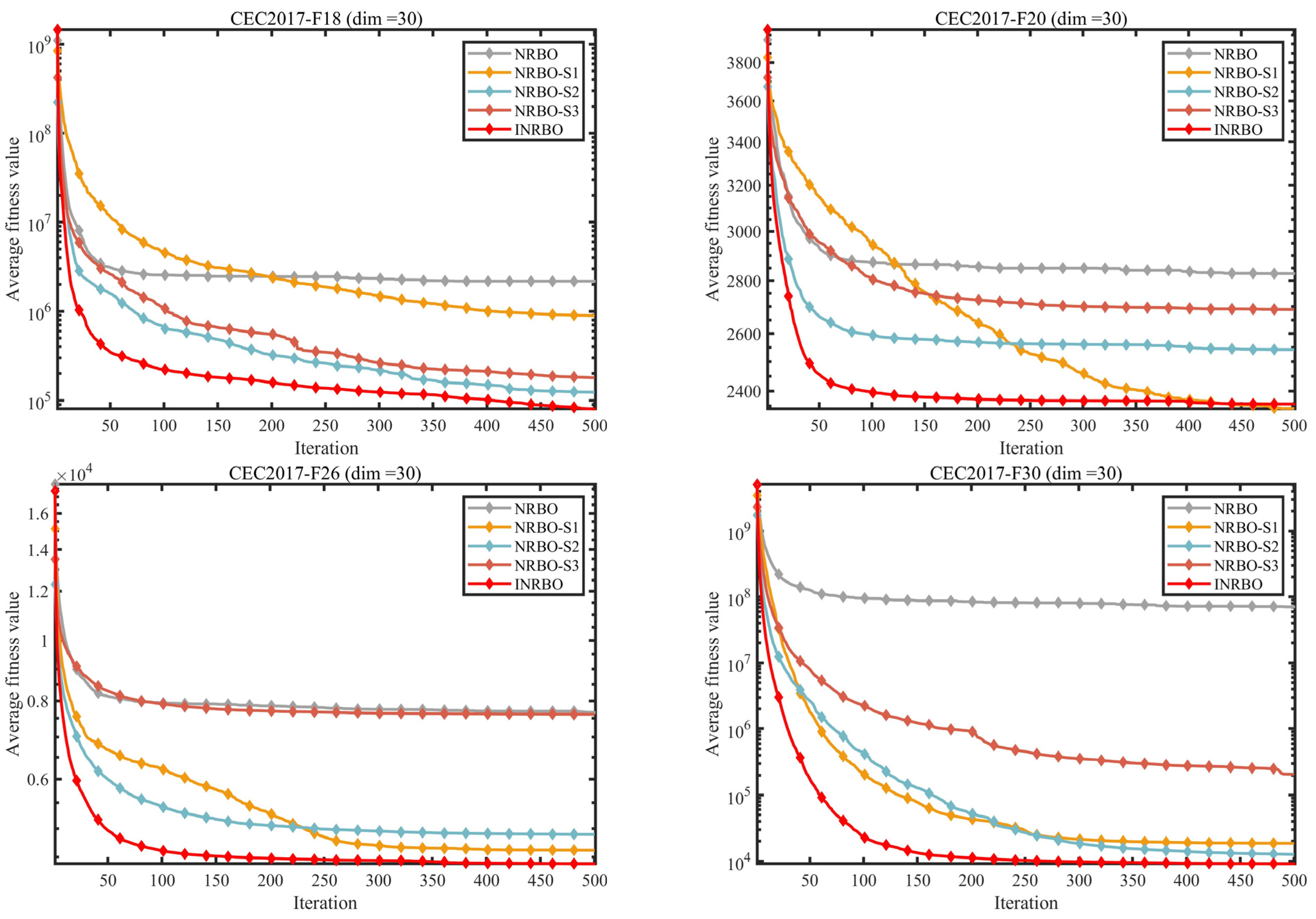
To evaluate the performance improvements brought by the proposed strategies—Adaptive Difference Operator Strategy, Quadratic Interpolation Strategy, and Elitist Population Genetic Strategy—an ablation study was conducted. This study compares the standard NRBO algorithm with three variants, each incorporating only a single strategy: NRBO-S1 (only Adaptive Difference Operator Strategy), NRBO-S2 (only Quadratic Interpolation Strategy), and NRBO-S3 (only Elitist Population Genetic Strategy). The comparison aims to quantify the individual contribution of each strategy and assess the combined effect in the full INRBO algorithm. The experiments were conducted on the CEC2017 benchmark set ($dim$ = 30), with parameters configured as described previously.

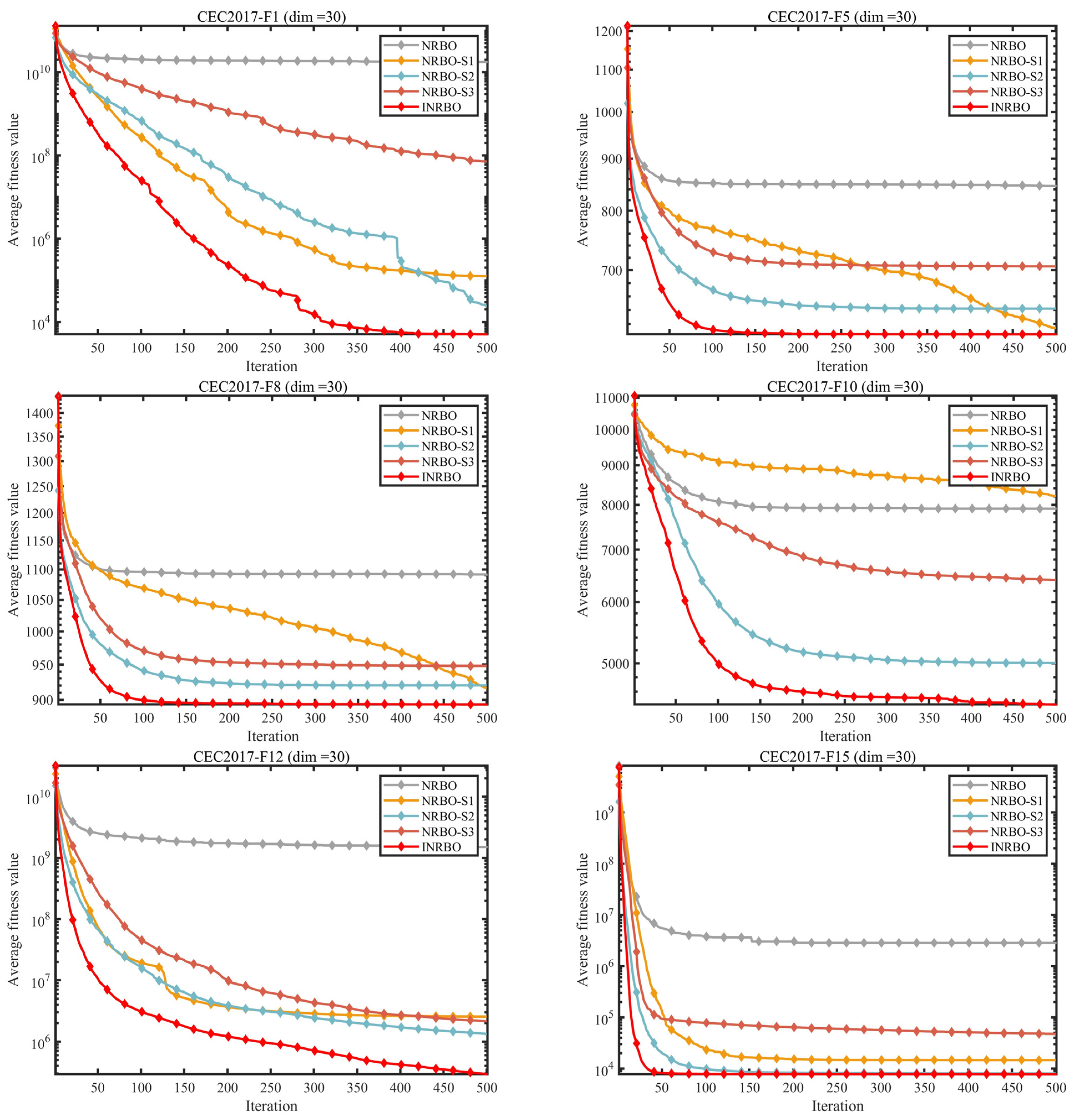
From Figure 1, unimodal functions have a single global optimum, so local refinement capability is the key to improving performance. The quadratic interpolation strategy (S2) plays a dominant role here. For F1 (Sphere function, typical unimodal), NRBO-S2 achieves a final fitness that is 22% lower than the original NRBO, while NRBO-S1 (adaptive differential operator) reduces fitness by only 15% and NRBO-S3 (elitist genetic) by 10%. This is because S2 leverages fitness information from the current solution, elite individuals, and the global best to construct a quadratic interpolation model. It enables directional prediction of optimal positions, reducing randomness in local search and significantly improving refinement accuracy.

On F5 (Rotated Rosenbrock function), another representative unimodal function, NRBO-S2’s convergence curve is consistently below those of S1 and S3. Its mean fitness is 6.2% lower than S1 and 8.7% lower than S3. The standard deviation of NRBO-S2 is also the smallest among the three single-strategy variants, indicating that S2 enhances both precision and stability in local exploitation. The adaptive differential operator (S1) contributes moderately to unimodal functions by adjusting the scaling factor, but its focus on balancing global and local search makes it less effective than S2 in the late-stage refinement that unimodal functions demand. The elitist genetic strategy (S3) has the weakest performance on unimodal functions, as its strength in inheriting high-quality genes is less critical when there is no need to escape local optima.

Multimodal functions contain multiple local optima, requiring strong global exploration to escape local traps. Here, the adaptive differential operator (S1) and elitist population genetic strategy (S3) are more dominant, while the quadratic interpolation strategy (S2) plays a supplementary role. For F10 (Schwefel’s function, a classic multimodal function with numerous local minima), NRBO-S1 shows the most significant improvement over the original NRBO—its final fitness is 28% lower, compared to 18% for S3 and 12% for S2. The dynamically decaying scaling factor in S1 enables large-step global exploration in early iterations, helping the algorithm jump out of local optima, while late-stage small-step exploitation refines solutions without stagnation.

NRBO-S3 also performs well on F10, with a convergence curve that avoids the plateau seen in NRBO and S2. By constructing an elite pool and preserving high-quality genes through crossover and mutation, S3 maintains population diversity, preventing premature convergence to local optima. For F12 (Rotated Ackley function), S1 and S3 show synergistic advantages: NRBO-S1 excels in exploring new regions, and NRBO-S3 ensures the inheritance of effective search directions. In contrast, S2’s local refinement capability is less useful in multimodal functions, as excessive focus on local areas can trap the algorithm in suboptimal solutions. Its contribution is limited to fine-tuning solutions after the global optimum region is identified.

The full INRBO algorithm integrates the advantages of all three strategies, achieving superior performance across both function types. For unimodal functions, INRBO combines S2’s local refinement with S1’s dynamic step adjustment and S3’s elite gene preservation. This results in a final fitness on F1 that is two orders of magnitude lower than the best single-strategy variant (NRBO-S2), demonstrating that S2’s dominant local refinement is enhanced by the other two strategies. For multimodal functions like F10, INRBO leverages S1’s global exploration and S3’s diversity maintenance to escape local optima, while S2 fine-tunes the solution once the global optimum region is found. This synergy leads to a fitness that is 35% lower than the best single-strategy variant (NRBO-S1).

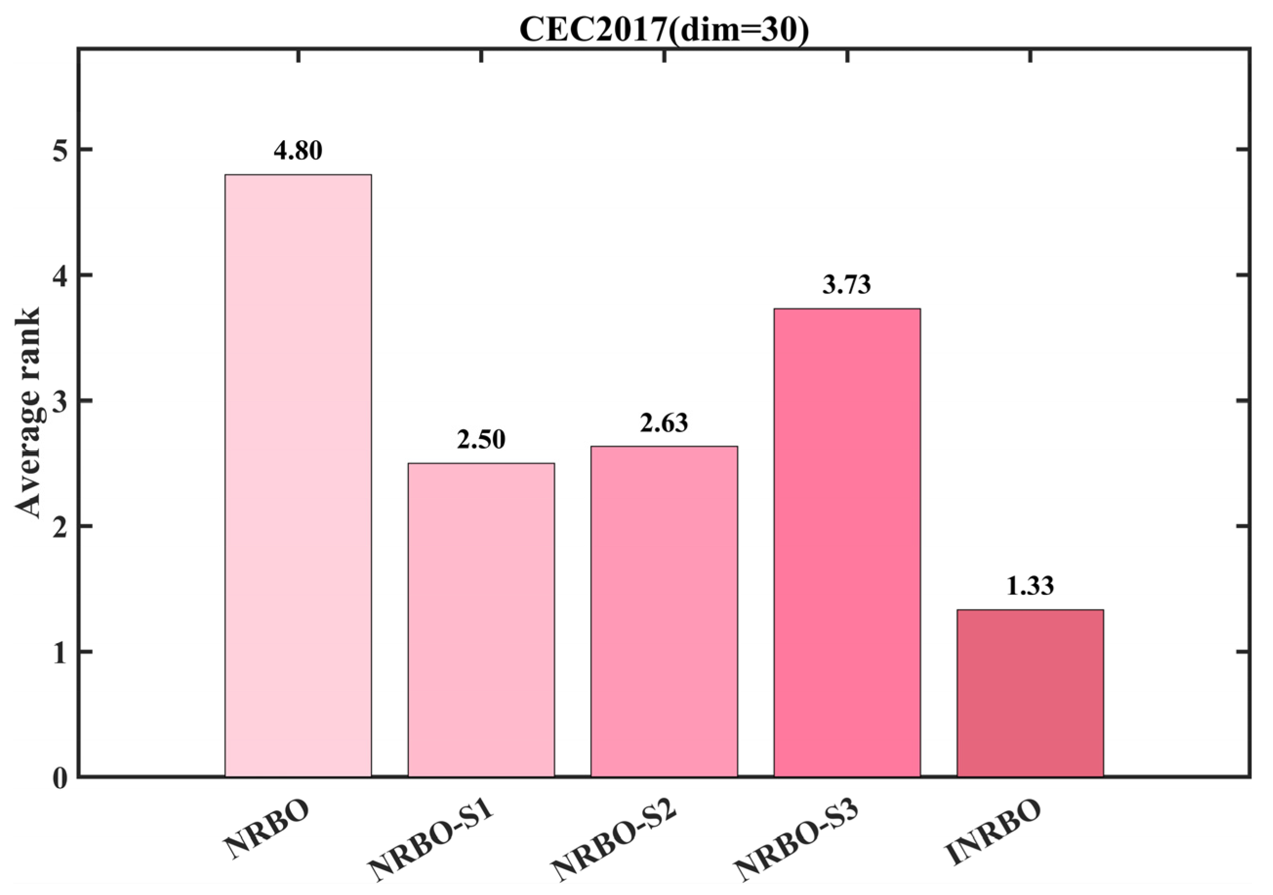
The average ranking results (Figure 2) further confirm this pattern. NRBO-S2 ranks second (2.63) overall, with its strength concentrated in unimodal functions, while NRBO-S1 (2.50) and NRBO-S3 (3.73) perform better in multimodal functions. INRBO achieves the top average rank (1.33) by integrating these complementary strengths, confirming that the three strategies form a synergistic framework tailored to different function characteristics.

3.3. Experimental Results and Analysis of CEC2017

This section evaluates the performance of the INRBO method against mainstream benchmark algorithms using the CEC2017 test suite, which includes four types of mathematical functions: unimodal, multimodal, hybrid, and composite. Multimodal functions, containing multiple local optima, are primarily used to assess global exploration ability, while unimodal functions, with a single global optimum, evaluate local exploitation efficiency. Hybrid and composite functions create more complex landscapes, testing the algorithm’s capacity to escape local optima.

To ensure fairness and minimize randomness, all algorithms were configured with the same parameters: a population size of 30 and a maximum of 500 iterations. Each algorithm was independently executed 30 times, and results were recorded as average (Ave) and standard deviation (Std), with the best values highlighted in bold.

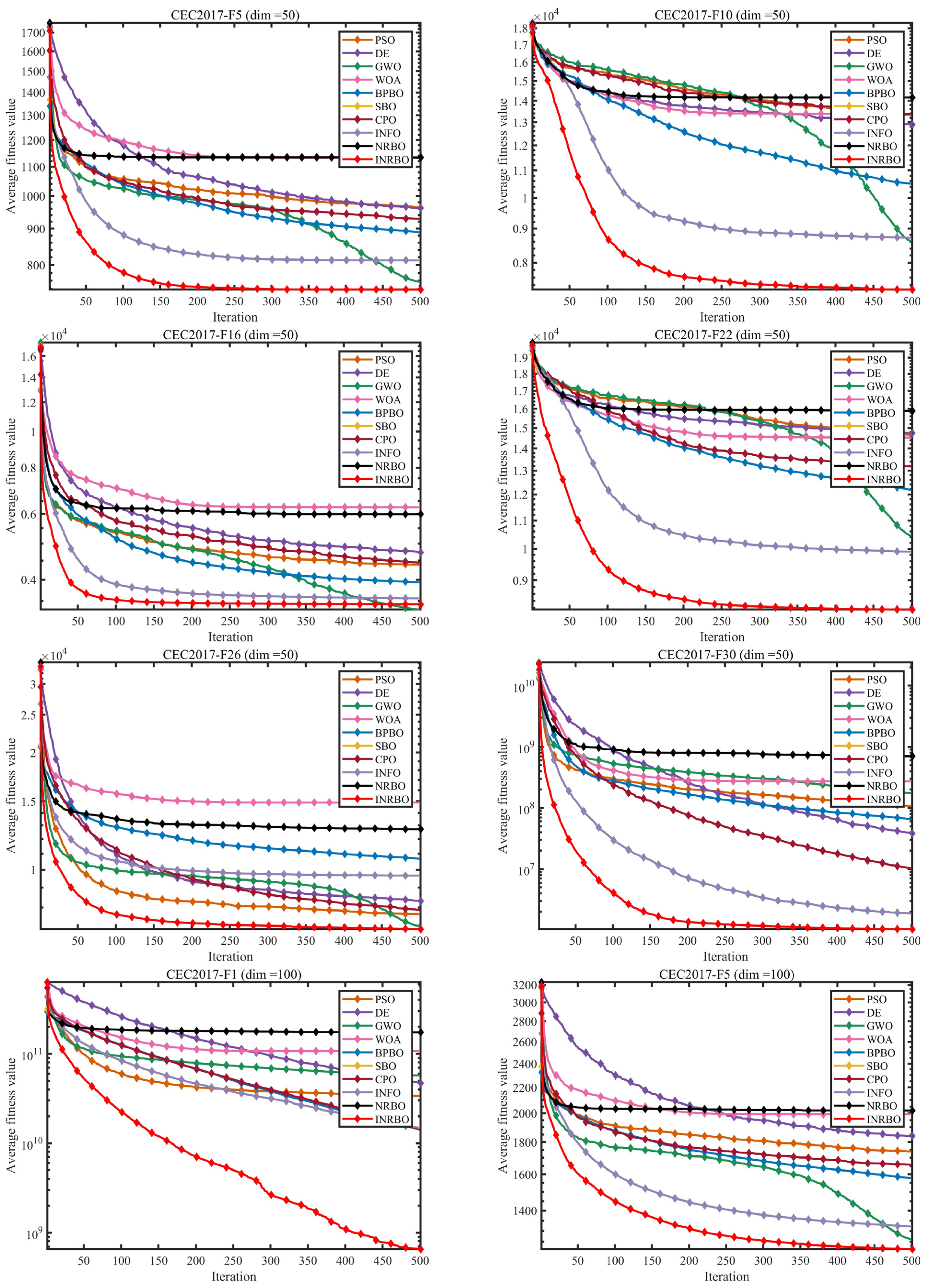
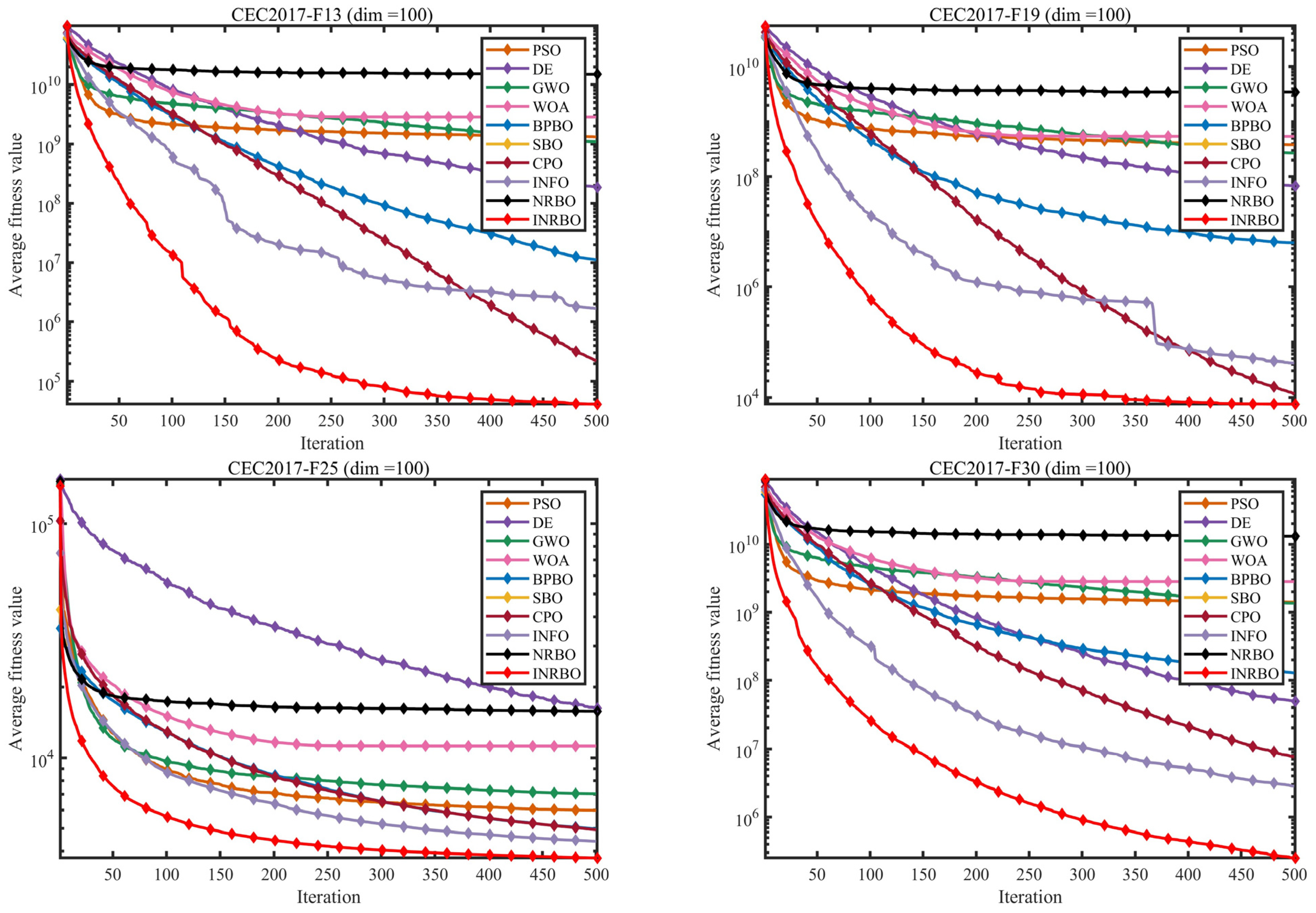
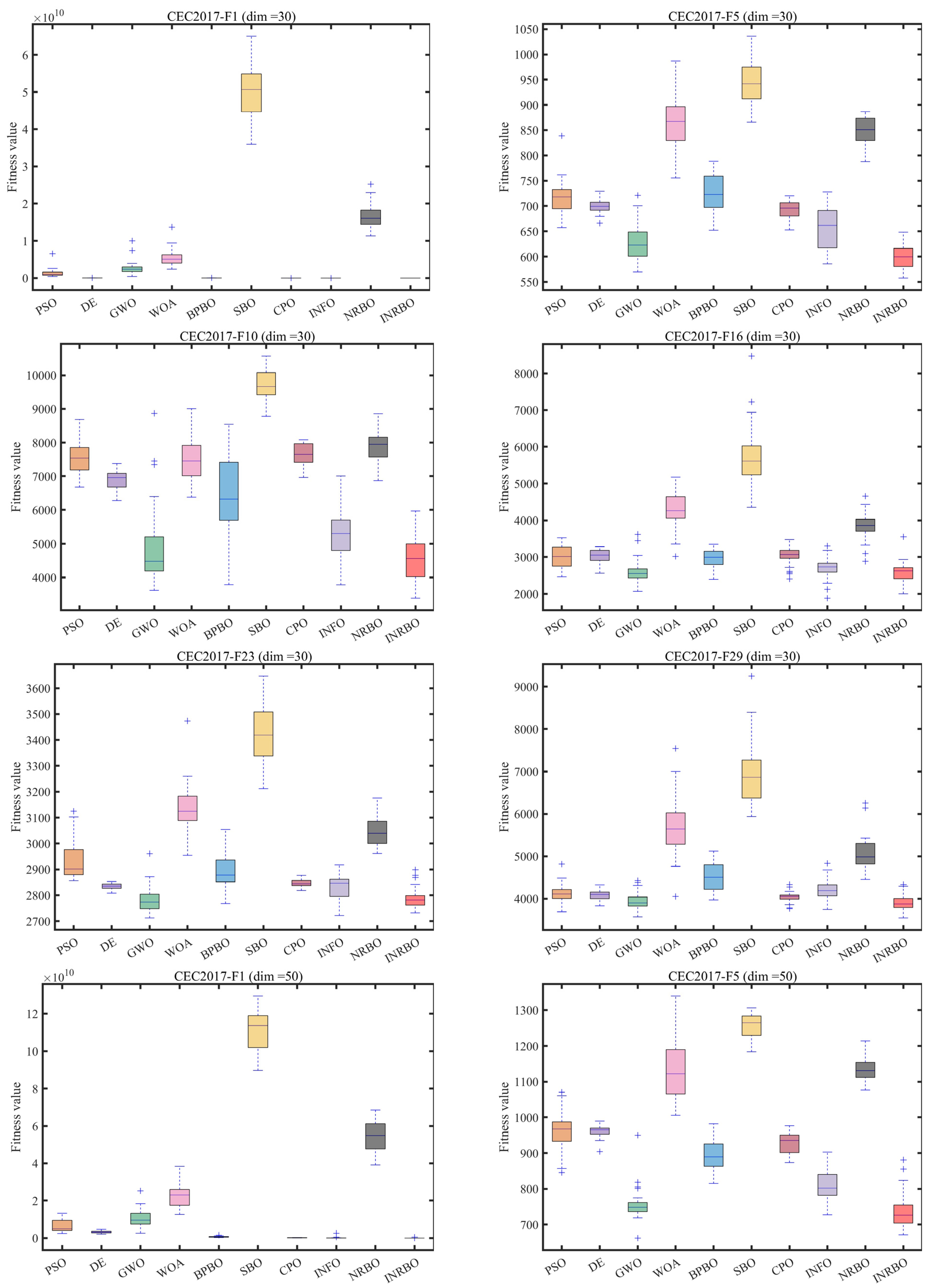
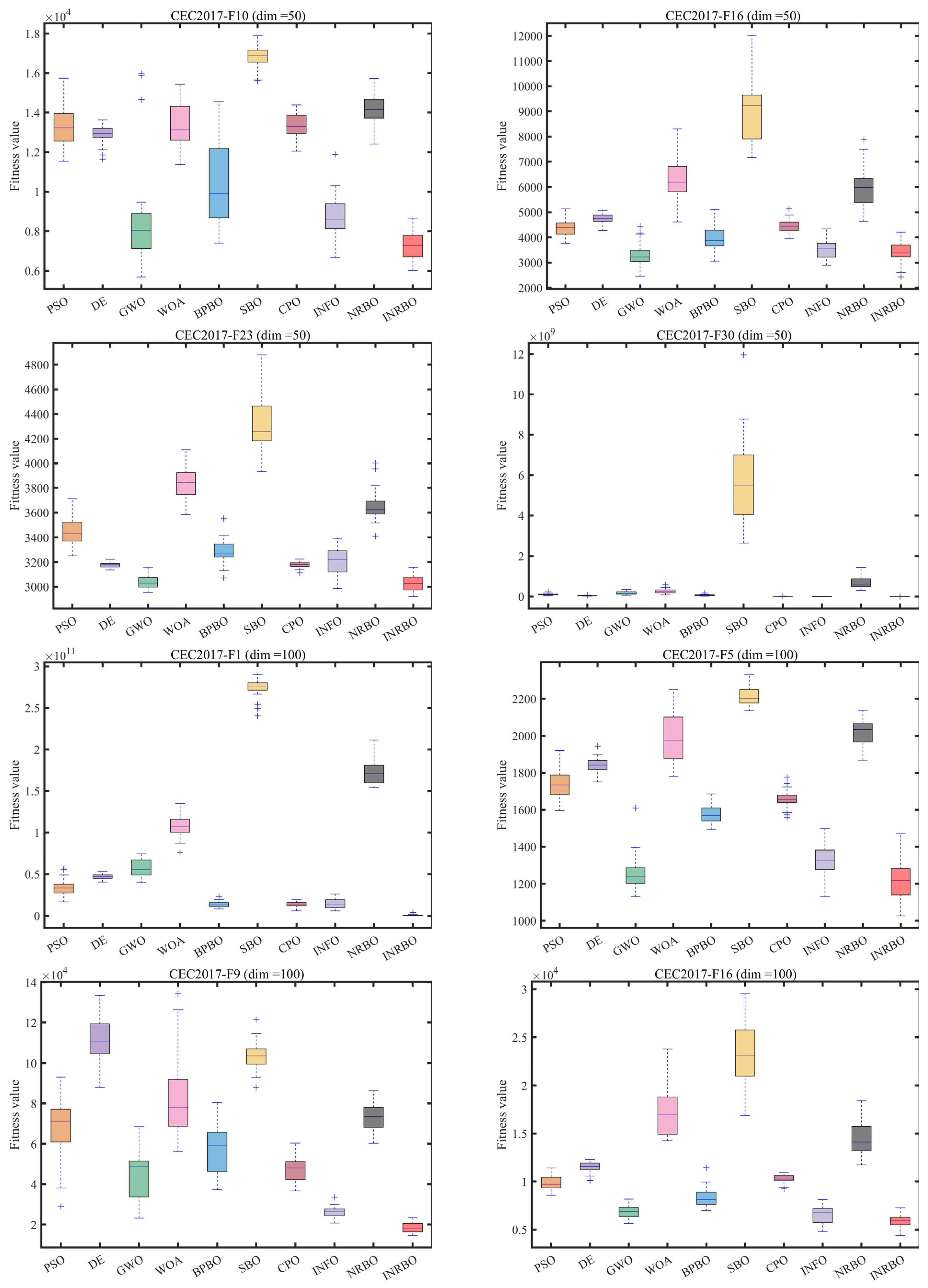
All experiments were conducted on a Windows 11 Professional (22H2) system, equipped with an AMD Ryzen 7 7700X 4.5 GHz eight-core CPU, 32 GB DDR5-6000 dual-channel RAM, NVIDIA GeForce RTX 4070 Ti 12 GB GDDR6X GPU, X670E chipset motherboard, and 2 TB WD SN850X NVMe PCIe 4.0 SSD. Cooling was provided by a 360 mm all-in-one liquid cooler, and the power supply was an 850 W gold-certified unit. Simulations were carried out in MATLAB R2024b, with the Parallel Computing Toolbox enabled to improve computation efficiency. Experimental results are presented in

Table 2. Results of CEC2017 benchmark evaluation (dim = 30).

Function	Metric	PSO	DE	GWO	WOA	BPBO	SBO	CPO	INFO	NRBO	INRBO
F1	Ave	1.3647 E + 09	3.1357 E + 07	2.6810 E + 09	5.2755 E + 09	2.7414 E + 07	5.0191 E + 10	6.2216 E + 05	1.3205 E + 05	1.6742 E + 10	5.7434 E + 03
	Std	1.1290 E + 09	8.6804 E + 06	1.8891 E + 09	2.2268 E + 09	1.5699 E + 07	7.2366 E + 09	4.1894 E + 05	6.3553 E + 05	3.5366 E + 09	6.5930 E + 03
F2	Ave	2.8282 E + 33	5.6600 E + 30	1.0852 E + 32	8.0717 E + 35	1.7271 E + 22	2.4687 E + 46	3.1088 E + 21	6.0436 E + 23	1.9620 E + 36	3.3394 E + 14
	Std	1.5490 E + 34	1.4892 E + 31	3.3741 E + 32	2.3751 E + 36	6.4550 E + 22	8.6579 E + 46	1.5527 E + 22	2.8976 E + 24	7.2718 E + 36	1.4227 E + 15
F3	Ave	6.2412 E + 04	1.7156 E + 05	6.5254 E + 04	2.8358 E + 05	5.1660 E + 04	1.3920 E + 05	6.5379 E + 04	1.5818 E + 04	5.6910 E + 04	2.1918 E + 03
	Std	2.3197 E + 04	2.4555 E + 04	1.1936 E + 04	6.8105 E + 04	6.6943 E + 03	5.5937 E + 04	1.1100 E + 04	5.9800 E + 03	9.0525 E + 03	1.4537 E + 03
F4	Ave	6.6446 E + 02	5.7128 E + 02	6.8064 E + 02	1.2500 E + 03	5.4224 E + 02	1.4298 E + 04	5.2098 E + 02	5.0225 E + 02	1.9222 E + 03	4.8166 E + 02
	Std	1.7843 E + 02	1.7005 E + 01	2.8619 E + 02	2.8954 E + 02	2.6959 E + 01	3.4854 E + 03	1.7698 E + 01	2.4732 E + 01	7.7287 E + 02	3.1088 E + 01
F5	Ave	7.1828 E + 02	6.9990 E + 02	6.2739 E + 02	8.6425 E + 02	7.2337 E + 02	9.4424 E + 02	6.9363 E + 02	6.5608 E + 02	8.4797 E + 02	6.0016 E + 02
	Std	3.4074 E + 01	1.3594 E + 01	3.5132 E + 01	5.1370 E + 01	3.7016 E + 01	4.2490 E + 01	1.5847 E + 01	4.0134 E + 01	2.8318 E + 01	2.5667 E + 01
F6	Ave	6.2129 E + 02	6.0395 E + 02	6.1101 E + 02	6.8047 E + 02	6.5425 E + 02	6.9962 E + 02	6.0176 E + 02	6.3031 E + 02	6.6969 E + 02	6.0656 E + 02
	Std	7.4038 E + 00	6.2926 E − 01	3.9559 E + 00	1.2719 E + 01	8.9918 E + 00	9.0914 E + 00	6.0460 E − 01	1.0899 E + 01	9.0584 E + 00	4.4283 E + 00
F7	Ave	9.8916 E + 02	9.4902 E + 02	9.2388 E + 02	1.3323 E + 03	1.1323 E + 03	1.4773 E + 03	9.3875 E + 02	9.7072 E + 02	1.2401 E + 03	8.8669 E + 02
	Std	2.5391 E + 01	1.3543 E + 01	5.8752 E + 01	9.1794 E + 01	8.7707 E + 01	6.5629 E + 01	1.8442 E + 01	5.6312 E + 01	8.2271 E + 01	5.4409 E + 01
F8	Ave	1.0101 E + 03	1.0035 E + 03	9.1653 E + 02	1.0707 E + 03	9.6356 E + 02	1.1897 E + 03	9.8078 E + 02	9.2245 E + 02	1.0897 E + 03	8.9900 E + 02
	Std	2.6897 E + 01	1.6047 E + 01	4.8216 E + 01	5.5503 E + 01	2.9816 E + 01	2.5558 E + 01	2.0316 E + 01	3.0866 E + 01	3.1391 E + 01	2.0215 E + 01
F9	Ave	1.8433 E + 03	5.1891 E + 03	2.5337 E + 03	1.3250 E + 04	5.9789 E + 03	1.4475 E + 04	1.2547 E + 03	3.2578 E + 03	7.3875 E + 03	1.5459 E + 03
	Std	8.1467 E + 02	8.3407 E + 02	8.3785 E + 02	5.7515 E + 03	1.5940 E + 03	2.4938 E + 03	2.9040 E + 02	6.4887 E + 02	1.4810 E + 03	6.0064 E + 02
F10	Ave	7.5317 E + 03	6.8790 E + 03	4.9215 E + 03	7.4985 E + 03	6.4297 E + 03	9.6997 E + 03	7.6294 E + 03	5.3295 E + 03	7.8861 E + 03	4.5457 E + 03
	Std	5.0055 E + 02	2.8275 E + 02	1.1959 E + 03	6.4580 E + 02	1.2998 E + 03	4.4744 E + 02	3.4997 E + 02	7.7852 E + 02	4.6605 E + 02	6.2345 E + 02
F11	Ave	1.5178 E + 03	3.1465 E + 03	2.7943 E + 03	1.0485 E + 04	1.3206 E + 03	1.8001 E + 04	1.2680 E + 03	1.2649 E + 03	2.6900 E + 03	1.2271 E + 03
	Std	2.1037 E + 02	1.1054 E + 03	1.6374 E + 03	3.5040 E + 03	4.8037 E + 01	7.0117 E + 03	2.4998 E + 01	5.3115 E + 01	7.3617 E + 02	4.7908 E + 01
F12	Ave	8.1026 E + 07	5.5286 E + 07	1.8084 E + 08	4.6089 E + 08	1.2564 E + 07	1.0050 E + 10	1.1333 E + 06	9.7126 E + 05	1.6424 E + 09	3.1402 E + 05
	Std	8.7289 E + 07	1.9453 E + 07	3.9705 E + 08	3.1874 E + 08	1.0951 E + 07	3.6452 E + 09	7.4425 E + 05	1.0810 E + 06	8.5710 E + 08	3.1014 E + 05
F13	Ave	6.5724 E + 06	1.3988 E + 07	2.8335 E + 07	1.0880 E + 07	1.4127 E + 05	6.9278 E + 09	2.3793 E + 04	2.1069 E + 04	3.8354 E + 08	1.3858 E + 04
	Std	1.2650 E + 07	8.8258 E + 06	8.5270 E + 07	9.1165 E + 06	1.4531 E + 05	3.4583 E + 09	1.4562 E + 04	1.9660 E + 04	2.6767 E + 08	1.4015 E + 04
F14	Ave	1.1018 E + 05	6.6821 E + 05	6.8053 E + 05	3.3474 E + 06	1.0092 E + 05	7.1609 E + 06	2.0792 E + 03	1.3863 E + 04	2.9734 E + 05	8.5769 E + 03
	Std	1.0278 E + 05	5.0750 E + 05	8.8302 E + 05	3.8571 E + 06	8.1694 E + 04	4.2138 E + 06	8.6723 E + 02	2.0121 E + 04	4.0266 E + 05	6.2297 E + 03
F15	Ave	1.4044 E + 05	2.5142 E + 06	1.8432 E + 06	6.7603 E + 06	1.5199 E + 04	8.0922 E + 08	3.8540 E + 03	1.2100 E + 04	1.8392 E + 06	7.0187 E + 03
	Std	8.8353 E + 04	1.9517 E + 06	6.9143 E + 06	7.3614 E + 06	7.5202 E + 03	4.4440 E + 08	1.4271 E + 03	1.0229 E + 04	4.4763 E + 06	5.9607 E + 03
F16	Ave	3.0053 E + 03	3.0193 E + 03	2.6079 E + 03	4.2536 E + 03	2.9497 E + 03	5.6982 E + 03	3.0377 E + 03	2.7011 E + 03	3.8528 E + 03	2.5828 E + 03
	Std	3.0538 E + 02	2.0843 E + 02	3.5222 E + 02	5.1512 E + 02	2.8794 E + 02	8.0447 E + 02	2.5545 E + 02	2.8920 E + 02	3.7535 E + 02	3.0643 E + 02
F17	Ave	2.1714 E + 03	2.3012 E + 03	2.1165 E + 03	2.8082 E + 03	2.4862 E + 03	3.7103 E + 03	2.0925 E + 03	2.3093 E + 03	2.6276 E + 03	2.0771 E + 03
	Std	2.0103 E + 02	1.1358 E + 02	2.0967 E + 02	2.8399 E + 02	2.6188 E + 02	3.9416 E + 02	1.1170 E + 02	2.1750 E + 02	2.4461 E + 02	1.5965 E + 02
F18	Ave	1.8246 E + 06	3.1373 E + 06	2.8186 E + 06	1.3194 E + 07	8.8033 E + 05	8.8778 E + 07	1.4823 E + 05	1.8198 E + 05	1.7972 E + 06	6.7919 E + 04
	Std	1.6517 E + 06	1.5410 E + 06	5.1979 E + 06	1.1898 E + 07	1.0469 E + 06	7.6989 E + 07	8.5418 E + 04	2.0584 E + 05	1.9980 E + 06	5.4796 E + 04
F19	Ave	8.3191 E + 05	2.1529 E + 06	2.5348 E + 06	2.4691 E + 07	1.3387 E + 05	9.5764 E + 08	6.6321 E + 03	1.3493 E + 04	1.4507 E + 07	1.0548 E + 04
	Std	2.2459 E + 06	1.4522 E + 06	7.0606 E + 06	2.1315 E + 07	3.4851 E + 05	5.4614 E + 08	4.6551 E + 03	1.4204 E + 04	1.6263 E + 07	1.1294 E + 04
F20	Ave	2.5502 E + 03	2.5817 E + 03	2.4896 E + 03	2.9988 E + 03	2.6290 E + 03	3.4623 E + 03	2.4691 E + 03	2.6145 E + 03	2.8217 E + 03	2.3705 E + 03
	Std	2.0879 E + 02	1.3273 E + 02	1.4554 E + 02	2.2767 E + 02	1.7466 E + 02	1.8194 E + 02	1.1226 E + 02	1.8455 E + 02	2.0171 E + 02	1.8477 E + 02
F21	Ave	2.5060 E + 03	2.4999 E + 03	2.4030 E + 03	2.6691 E + 03	2.4685 E + 03	2.7167 E + 03	2.4814 E + 03	2.4341 E + 03	2.6049 E + 03	2.4112 E + 03
	Std	2.7927 E + 01	1.6165 E + 01	2.1420 E + 01	6.3796 E + 01	4.3724 E + 01	4.9338 E + 01	1.8345 E + 01	2.8237 E + 01	5.1442 E + 01	3.4615 E + 01
F22	Ave	5.0322 E + 03	5.4577 E + 03	4.8251 E + 03	8.6435 E + 03	2.9950 E + 03	9.8448 E + 03	2.3090 E + 03	5.2198 E + 03	5.7986 E + 03	2.3019 E + 03
	Std	3.0506 E + 03	1.7863 E + 03	1.7248 E + 03	1.7341 E + 03	1.7105 E + 03	1.3327 E + 03	2.6811 E + 00	2.0504 E + 03	2.2977 E + 03	2.9708 E + 00
F23	Ave	2.9386 E + 03	2.8343 E + 03	2.7831 E + 03	3.1387 E + 03	2.8938 E + 03	3.4258 E + 03	2.8465 E + 03	2.8333 E + 03	3.0465 E + 03	2.7862 E + 03
	Std	7.6290 E + 01	1.2619 E + 01	5.3265 E + 01	9.6802 E + 01	6.3865 E + 01	1.1422 E + 02	1.4390 E + 01	4.8482 E + 01	5.5845 E + 01	4.2394 E + 01
F24	Ave	3.1016 E + 03	3.0541 E + 03	2.9663 E + 03	3.2505 E + 03	3.0149 E + 03	3.5864 E + 03	3.0172 E + 03	2.9815 E + 03	3.2105 E + 03	2.9637 E + 03
	Std	5.1920 E + 01	1.5271 E + 01	7.8649 E + 01	9.2995 E + 01	5.1815 E + 01	1.3656 E + 02	1.8246 E + 01	5.8114 E + 01	5.8411 E + 01	3.9805 E + 01
F25	Ave	2.9702 E + 03	2.9669 E + 03	3.0159 E + 03	3.2400 E + 03	2.9746 E + 03	5.5451 E + 03	2.9148 E + 03	2.9100 E + 03	3.3747 E + 03	2.8975 E + 03
	Std	2.6059 E + 01	1.8163 E + 01	4.1700 E + 01	7.0012 E + 01	2.4459 E + 01	7.4846 E + 02	1.7605 E + 01	1.8564 E + 01	1.6952 E + 02	1.6617 E + 01
F26	Ave	5.1601 E + 03	5.5595 E + 03	4.9765 E + 03	8.2569 E + 03	6.4954 E + 03	1.0732 E + 04	4.5498 E + 03	5.7525 E + 03	8.0335 E + 03	4.2076 E + 03
	Std	1.0850 E + 03	1.2421 E + 02	4.0835 E + 02	1.1611 E + 03	1.9567 E + 03	7.1838 E + 02	1.3279 E + 03	1.2533 E + 03	9.3841 E + 02	1.2872 E + 03
F27	Ave	3.2686 E + 03	3.2354 E + 03	3.2663 E + 03	3.4552 E + 03	3.3719 E + 03	4.1379 E + 03	3.2807 E + 03	3.2676 E + 03	3.4638 E + 03	3.2400 E + 03
	Std	4.4542 E + 01	5.2071 E + 00	2.5819 E + 01	1.2387 E + 02	9.7299 E + 01	2.1715 E + 02	1.3481 E + 01	4.3360 E + 01	1.2213 E + 02	2.6848 E + 01
F28	Ave	3.3926 E + 03	3.3961 E + 03	3.4861 E + 03	3.9124 E + 03	3.3248 E + 03	7.4148 E + 03	3.2792 E + 03	3.2584 E + 03	4.1388 E + 03	3.2209 E + 03
	Std	1.6548 E + 02	3.5101 E + 01	1.0122 E + 02	2.3196 E + 02	2.7518 E + 01	8.3529 E + 02	2.5444 E + 01	3.1782 E + 01	4.6536 E + 02	2.1785 E + 01
F29	Ave	4.1403 E + 03	4.0848 E + 03	3.9298 E + 03	5.7004 E + 03	4.5150 E + 03	6.9703 E + 03	4.0362 E + 03	4.1910 E + 03	5.0835 E + 03	3.9021 E + 03
	Std	2.2269 E + 02	1.1779 E + 02	2.0827 E + 02	7.3200 E + 02	3.3382 E + 02	7.6394 E + 02	1.2620 E + 02	2.5837 E + 02	4.0157 E + 02	1.9398 E + 02
F30	Ave	2.3461 E + 06	1.8121 E + 06	1.3504 E + 07	5.7718 E + 07	1.1395 E + 06	8.9847 E + 08	1.1472 E + 05	2.3194 E + 04	9.0653 E + 07	8.7455 E + 03
	Std	1.7601 E + 06	1.1860 E + 06	1.1624 E + 07	4.9269 E + 07	9.6395 E + 05	5.8133 E + 08	6.3214 E + 04	2.3065 E + 04	5.0178 E + 07	2.5375 E + 03

,

Table 3. Results of CEC2017 benchmark evaluation (dim = 50).

Function	Metric	PSO	DE	GWO	WOA	BPBO	SBO	CPO	INFO	NRBO	INRBO
F1	Ave	6.2444 E + 09	3.2364 E + 09	1.0413 E + 10	2.2587 E + 10	6.6549 E + 08	1.1178 E + 11	1.7281 E + 08	1.4162 E + 08	5.4798 E + 10	1.7755 E + 07
	Std	3.0806 E + 09	6.8576 E + 08	4.5778 E + 09	5.8728 E + 09	2.7709 E + 08	1.0560 E + 10	6.6128 E + 07	4.6351 E + 08	7.3456 E + 09	8.9880 E + 07
F2	Ave	2.9882 E + 57	5.7654 E + 63	7.5931 E + 53	1.1242 E + 84	8.1164 E + 55	2.4405 E + 83	1.1244 E + 45	2.8758 E + 48	3.1006 E + 69	1.0595 E + 39
	Std	1.6367 E + 58	1.8636 E + 64	2.8634 E + 54	6.1574 E + 84	4.3800 E + 56	1.2976 E + 84	2.9912 E + 45	1.2110 E + 49	1.6982 E + 70	5.7811 E + 39
F3	Ave	1.9697 E + 05	3.4547 E + 05	1.8108 E + 05	2.6311 E + 05	1.5110 E + 05	5.1111 E + 05	1.8155 E + 05	1.1875 E + 05	1.7456 E + 05	3.5868 E + 04
	Std	6.6508 E + 04	4.5109 E + 04	3.5140 E + 04	6.7448 E + 04	1.9665 E + 04	3.0904 E + 05	1.7728 E + 04	3.5691 E + 04	3.1057 E + 04	7.2834 E + 03
F4	Ave	1.1174 E + 03	1.1643 E + 03	1.5570 E + 03	4.2871 E + 03	8.6170 E + 02	3.6318 E + 04	7.2825 E + 02	6.5655 E + 02	9.1015 E + 03	5.6052 E + 02
	Std	3.3655 E + 02	1.0890 E + 02	5.7231 E + 02	9.2594 E + 02	8.9325 E + 01	5.5568 E + 03	6.3204 E + 01	8.3557 E + 01	2.1078 E + 03	3.9549 E + 01
F5	Ave	9.6490 E + 02	9.6168 E + 02	7.5740 E + 02	1.1328 E + 03	8.8913 E + 02	1.2598 E + 03	9.2860 E + 02	8.1227 E + 02	1.1336 E + 03	7.3865 E + 02
	Std	5.1899 E + 01	1.7840 E + 01	4.6078 E + 01	8.9274 E + 01	4.4054 E + 01	3.0279 E + 01	2.7610 E + 01	4.8656 E + 01	3.4337 E + 01	5.1101 E + 01
F6	Ave	6.4231 E + 02	6.1771 E + 02	6.2449 E + 02	6.9702 E + 02	6.6795 E + 02	7.1454 E + 02	6.1021 E + 02	6.4314 E + 02	6.8917 E + 02	6.2379 E + 02
	Std	1.3632 E + 01	2.3467 E + 00	5.6059 E + 00	1.3227 E + 01	7.3197 E + 00	8.4808 E + 00	2.4709 E + 00	8.5739 E + 00	8.1660 E + 00	5.8787 E + 00
F7	Ave	1.3233 E + 03	1.2989 E + 03	1.1644 E + 03	1.8657 E + 03	1.7027 E + 03	2.1389 E + 03	1.2446 E + 03	1.4025 E + 03	1.8120 E + 03	1.1237 E + 03
	Std	4.2863 E + 01	3.1698 E + 01	6.2205 E + 01	1.0342 E + 02	9.9192 E + 01	6.5617 E + 01	3.5428 E + 01	1.1932 E + 02	1.0640 E + 02	7.1545 E + 01
F8	Ave	1.2619 E + 03	1.2621 E + 03	1.0687 E + 03	1.4044 E + 03	1.2231 E + 03	1.5836 E + 03	1.2208 E + 03	1.0940 E + 03	1.4461 E + 03	1.0677 E + 03
	Std	4.8351 E + 01	2.3096 E + 01	7.6337 E + 01	7.1638 E + 01	3.7238 E + 01	3.8648 E + 01	2.2770 E + 01	5.2442 E + 01	5.0133 E + 01	4.3691 E + 01
F9	Ave	1.2149 E + 04	2.1972 E + 04	1.3585 E + 04	4.0196 E + 04	2.5379 E + 04	5.0270 E + 04	7.3875 E + 03	9.0088 E + 03	2.8675 E + 04	4.4397 E + 03
	Std	7.4918 E + 03	3.4598 E + 03	5.6746 E + 03	1.2729 E + 04	6.3962 E + 03	5.9173 E + 03	2.9258 E + 03	1.8443 E + 03	3.7337 E + 03	1.5274 E + 03
F10	Ave	1.3335 E + 04	1.2892 E + 04	8.6083 E + 03	1.3378 E + 04	1.0508 E + 04	1.6815 E + 04	1.3369 E + 04	8.7200 E + 03	1.4160 E + 04	7.2867 E + 03
	Std	1.0776 E + 03	4.6143 E + 02	2.5444 E + 03	1.1187 E + 03	2.0234 E + 03	5.4085 E + 02	6.3423 E + 02	1.0818 E + 03	7.1175 E + 02	7.0690 E + 02
F11	Ave	2.7495 E + 03	1.2111 E + 04	7.7096 E + 03	8.6574 E + 03	2.2773 E + 03	3.2384 E + 04	1.8308 E + 03	1.4631 E + 03	9.2981 E + 03	1.3464 E + 03
	Std	4.5716 E + 02	3.4300 E + 03	3.3512 E + 03	2.6478 E + 03	3.2355 E + 02	7.6292 E + 03	2.2510 E + 02	1.7630 E + 02	2.6883 E + 03	5.3327 E + 01
F12	Ave	2.3983 E + 09	1.0663 E + 09	1.6887 E + 09	4.3741 E + 09	1.1038 E + 08	6.5172 E + 10	1.7413 E + 07	1.5693 E + 07	1.6962 E + 10	4.2335 E + 06
	Std	2.3216 E + 09	2.0668 E + 08	1.9256 E + 09	1.7482 E + 09	6.7332 E + 07	1.4770 E + 10	7.0716 E + 06	1.3997 E + 07	5.1697 E + 09	2.3574 E + 06
F13	Ave	2.2443 E + 08	6.7631 E + 07	1.9579 E + 08	5.1271 E + 08	1.3481 E + 06	3.0401 E + 10	1.6238 E + 04	2.1537 E + 04	4.4177 E + 09	7.9143 E + 03
	Std	3.8053 E + 08	3.7188 E + 07	1.3238 E + 08	2.5621 E + 08	1.2912 E + 06	1.0205 E + 10	6.4083 E + 03	1.1299 E + 04	3.0124 E + 09	6.0048 E + 03
F14	Ave	8.5595 E + 05	4.4605 E + 06	1.3895 E + 06	9.2564 E + 06	7.0266 E + 05	8.8791 E + 07	1.3676 E + 05	1.0921 E + 05	3.5339 E + 06	6.1354 E + 04
	Std	8.7322 E + 05	2.3612 E + 06	1.4460 E + 06	7.8733 E + 06	5.6501 E + 05	4.5290 E + 07	1.1312 E + 05	9.0306 E + 04	3.3396 E + 06	5.6190 E + 04
F15	Ave	9.8310 E + 06	1.0226 E + 07	8.6072 E + 07	6.7149 E + 07	9.9940 E + 04	6.6127 E + 09	1.1350 E + 04	1.3277 E + 04	3.8113 E + 08	7.8998 E + 03
	Std	6.7876 E + 06	6.5433 E + 06	1.5773 E + 08	9.4136 E + 07	8.2738 E + 04	2.2626 E + 09	5.1856 E + 03	8.6471 E + 03	2.2557 E + 08	7.1436 E + 03
F16	Ave	4.3838 E + 03	4.7373 E + 03	3.3226 E + 03	6.2593 E + 03	3.9321 E + 03	9.0052 E + 03	4.4478 E + 03	3.5593 E + 03	5.9893 E + 03	3.4294 E + 03
	Std	3.5755 E + 02	2.0660 E + 02	4.4487 E + 02	8.4477 E + 02	4.8220 E + 02	1.2068 E + 03	2.7683 E + 02	3.7348 E + 02	8.0551 E + 02	4.3415 E + 02
F17	Ave	3.8549 E + 03	3.7846 E + 03	3.0621 E + 03	4.6174 E + 03	3.8316 E + 03	1.1442 E + 04	3.5593 E + 03	3.4551 E + 03	4.6412 E + 03	3.1104 E + 03
	Std	3.4435 E + 02	2.0307 E + 02	3.1361 E + 02	1.1037 E + 03	3.5796 E + 02	5.3615 E + 03	1.7723 E + 02	3.0727 E + 02	4.5555 E + 02	3.6954 E + 02
F18	Ave	6.7724 E + 06	1.8288 E + 07	1.0566 E + 07	5.4578 E + 07	3.0244 E + 06	2.7603 E + 08	2.3560 E + 06	6.3618 E + 05	2.3908 E + 07	2.2041 E + 05
	Std	3.8617 E + 06	5.7779 E + 06	1.0888 E + 07	4.3479 E + 07	2.1003 E + 06	1.5672 E + 08	1.7044 E + 06	5.8615 E + 05	1.9548 E + 07	1.7947 E + 05
F19	Ave	6.1894 E + 06	2.7139 E + 06	1.2602 E + 07	1.8675 E + 07	3.6444 E + 05	3.7974 E + 09	1.9900 E + 04	1.7258 E + 04	1.9068 E + 08	1.2594 E + 04
	Std	4.2684 E + 06	1.4673 E + 06	3.0455 E + 07	1.2211 E + 07	5.7069 E + 05	1.8826 E + 09	7.3863 E + 03	9.3068 E + 03	1.0544 E + 08	8.0697 E + 03
F20	Ave	3.5356 E + 03	3.6740 E + 03	3.1890 E + 03	4.0051 E + 03	3.3592 E + 03	4.9432 E + 03	3.6657 E + 03	3.4156 E + 03	3.8169 E + 03	3.0016 E + 03
	Std	2.9874 E + 02	1.6070 E + 02	4.1222 E + 02	2.8180 E + 02	4.2034 E + 02	2.7936 E + 02	1.9015 E + 02	3.5666 E + 02	2.6005 E + 02	3.4724 E + 02
F21	Ave	2.7543 E + 03	2.7667 E + 03	2.5550 E + 03	3.0435 E + 03	2.6687 E + 03	3.2036 E + 03	2.7013 E + 03	2.6119 E + 03	2.9822 E + 03	2.5240 E + 03
	Std	4.6561 E + 01	2.0214 E + 01	7.0155 E + 01	1.1172 E + 02	7.0187 E + 01	8.5626 E + 01	2.8090 E + 01	6.1143 E + 01	7.2374 E + 01	4.9779 E + 01
F22	Ave	1.4656 E + 04	1.4743 E + 04	1.0450 E + 04	1.4523 E + 04	1.2176 E + 04	1.8209 E + 04	1.3187 E + 04	9.9088 E + 03	1.5881 E + 04	8.1589 E + 03
	Std	2.2211 E + 03	5.1281 E + 02	2.7024 E + 03	1.1142 E + 03	1.7375 E + 03	8.0793 E + 02	4.8963 E + 03	9.0374 E + 02	8.2973 E + 02	2.4967 E + 03
F23	Ave	3.4401 E + 03	3.1765 E + 03	3.0349 E + 03	3.8338 E + 03	3.2833 E + 03	4.3072 E + 03	3.1795 E + 03	3.2120 E + 03	3.6559 E + 03	3.0259 E + 03
	Std	1.1442 E + 02	2.1652 E + 01	4.9463 E + 01	1.4919 E + 02	9.7675 E + 01	2.1509 E + 02	2.5400 E + 01	1.0428 E + 02	1.2236 E + 02	6.8804 E + 01
F24	Ave	3.5961 E + 03	3.3953 E + 03	3.2201 E + 03	3.9571 E + 03	3.3836 E + 03	4.5935 E + 03	3.3557 E + 03	3.3148 E + 03	3.7803 E + 03	3.2529 E + 03
	Std	1.1966 E + 02	2.0382 E + 01	8.8818 E + 01	1.4709 E + 02	1.0271 E + 02	2.1237 E + 02	3.0605 E + 01	1.0424 E + 02	1.0415 E + 02	9.5637 E + 01
F25	Ave	3.3788 E + 03	3.6723 E + 03	3.9758 E + 03	5.4173 E + 03	3.3374 E + 03	1.5968 E + 04	3.2373 E + 03	3.1615 E + 03	7.6280 E + 03	3.1042 E + 03
	Std	9.8744 E + 01	1.2189 E + 02	4.9733 E + 02	6.8301 E + 02	8.6556 E + 01	1.6404 E + 03	6.3458 E + 01	4.5287 E + 01	9.1958 E + 02	3.6116 E + 01
F26	Ave	7.6934 E + 03	8.3185 E + 03	7.1657 E + 03	1.4882 E + 04	1.0669 E + 04	1.8199 E + 04	7.8840 E + 03	9.6551 E + 03	1.2706 E + 04	7.0405 E + 03
	Std	1.9006 E + 03	2.1251 E + 02	5.8134 E + 02	1.3957 E + 03	2.1259 E + 03	8.2893 E + 02	2.0700 E + 03	1.6670 E + 03	1.4904 E + 03	2.3783 E + 03
F27	Ave	3.7346 E + 03	3.6231 E + 03	3.7276 E + 03	4.8757 E + 03	4.1324 E + 03	6.6111 E + 03	3.7394 E + 03	3.6802 E + 03	4.4924 E + 03	3.5748 E + 03
	Std	1.7262 E + 02	4.1289 E + 01	1.0591 E + 02	6.5358 E + 02	2.6979 E + 02	5.4055 E + 02	9.4427 E + 01	1.4402 E + 02	2.9456 E + 02	1.0216 E + 02
F28	Ave	3.8176 E + 03	6.2281 E + 03	4.4981 E + 03	6.3359 E + 03	3.7708 E + 03	1.3330 E + 04	3.6795 E + 03	3.5391 E + 03	7.2051 E + 03	3.3469 E + 03
	Std	5.1115 E + 02	6.2683 E + 02	4.4245 E + 02	5.1005 E + 02	1.0486 E + 02	1.5829 E + 03	7.8960 E + 01	8.4700 E + 01	8.2482 E + 02	3.8313 E + 01
F29	Ave	5.6088 E + 03	5.2951 E + 03	4.9847 E + 03	9.9597 E + 03	6.2149 E + 03	6.0406 E + 04	5.2491 E + 03	4.9234 E + 03	8.4790 E + 03	4.6943 E + 03
	Std	3.7423 E + 02	2.3180 E + 02	3.8949 E + 02	2.0804 E + 03	4.9099 E + 02	7.4976 E + 04	3.5510 E + 02	3.8943 E + 02	1.8502 E + 03	3.9477 E + 02
F30	Ave	1.0664 E + 08	3.8061 E + 07	1.7504 E + 08	2.7134 E + 08	6.5120 E + 07	5.6937 E + 09	1.0234 E + 07	1.8776 E + 06	7.0167 E + 08	1.0418 E + 06
	Std	4.2222 E + 07	1.1935 E + 07	7.2587 E + 07	1.1098 E + 08	3.4665 E + 07	2.1243 E + 09	3.4480 E + 06	7.5389 E + 05	3.0195 E + 08	1.9520 E + 05

and

Table 4. Results of CEC2017 benchmark evaluation (dim = 100).

Function	Metric	PSO	DE	GWO	WOA	BPBO	SBO	CPO	INFO	NRBO	INRBO
F1	Ave	3.3706 E + 10	4.7073 E + 10	5.7307 E + 10	1.0757 E + 11	1.4187 E + 10	2.7419 E + 11	1.4109 E + 10	1.4692 E + 10	1.7264 E + 11	6.5414 E + 08
	Std	9.2525 E + 09	3.1969 E + 09	1.0415 E + 10	1.2881 E + 10	3.3480 E + 09	1.0903 E + 10	3.2115 E + 09	5.7612 E + 09	1.4089 E + 10	9.7890 E + 08
F2	Ave	1.1493 E + 131	9.4200 E + 152	9.1772 E + 136	1.2938 E + 178	2.4409 E + 142	6.8664 E + 175	1.8047 E + 128	2.1131 E + 139	2.0769 E + 153	5.5558 E + 120
	Std	5.5546 E + 131	2.2362 E + 153	4.9422 E + 137	6.5535 E + 04	9.4480 E + 142	6.5535 E + 04	9.7098 E + 128	1.1219 E + 140	6.5535 E + 04	2.6692 E + 121
F3	Ave	5.9459 E + 05	8.3986 E + 05	5.6287 E + 05	9.3332 E + 05	3.3846 E + 05	6.6144 E + 06	4.6705 E + 05	3.8265 E + 05	3.8642 E + 05	2.0164 E + 05
	Std	1.2992 E + 05	8.7707 E + 04	7.5261 E + 04	1.2091 E + 05	1.6536 E + 04	1.5734 E + 07	5.6272 E + 04	6.6394 E + 04	6.7226 E + 04	2.0902 E + 04
F4	Ave	4.5353 E + 03	8.6397 E + 03	5.4716 E + 03	2.0968 E + 04	2.4769 E + 03	1.0480 E + 05	2.3114 E + 03	1.8393 E + 03	2.8978 E + 04	1.0586 E + 03
	Std	1.8165 E + 03	1.0722 E + 03	1.2474 E + 03	4.4448 E + 03	4.2985 E + 02	1.6635 E + 04	3.8060 E + 02	3.3668 E + 02	4.6639 E + 03	1.2626 E + 02
F5	Ave	1.7380 E + 03	1.8404 E + 03	1.2618 E + 03	1.9930 E + 03	1.5771 E + 03	2.2115 E + 03	1.6559 E + 03	1.3213 E + 03	2.0202 E + 03	1.2164 E + 03
	Std	8.7534 E + 01	4.1854 E + 01	9.3884 E + 01	1.3306 E + 02	5.1259 E + 01	5.0579 E + 01	5.0169 E + 01	8.0453 E + 01	6.6897 E + 01	1.0734 E + 02
F6	Ave	6.7398 E + 02	6.5135 E + 02	6.4651 E + 02	7.0801 E + 02	6.8123 E + 02	7.2120 E + 02	6.4140 E + 02	6.6011 E + 02	7.0525 E + 02	6.4436 E + 02
	Std	1.3149 E + 01	2.1492 E + 00	4.3008 E + 00	7.2946 E + 00	4.3728 E + 00	5.1041 E + 00	5.1575 E + 00	5.2636 E + 00	4.5676 E + 00	6.0368 E + 00
F7	Ave	2.4603 E + 03	3.2449 E + 03	2.2365 E + 03	3.8408 E + 03	3.4207 E + 03	4.1989 E + 03	2.3610 E + 03	2.8101 E + 03	3.7457 E + 03	2.2496 E + 03
	Std	1.4509 E + 02	1.1988 E + 02	1.2394 E + 02	1.7104 E + 02	1.7364 E + 02	1.0917 E + 02	1.1930 E + 02	2.4000 E + 02	1.9335 E + 02	1.5109 E + 02
F8	Ave	2.0032 E + 03	2.1076 E + 03	1.5338 E + 03	2.3997 E + 03	2.0174 E + 03	2.7022 E + 03	1.9687 E + 03	1.6892 E + 03	2.4771 E + 03	1.5392 E + 03
	Std	7.4991 E + 01	3.9915 E + 01	8.2578 E + 01	1.2179 E + 02	5.6673 E + 01	5.4345 E + 01	6.3948 E + 01	8.4993 E + 01	8.4148 E + 01	8.7453 E + 01
F9	Ave	6.9119 E + 04	1.1137 E + 05	4.4829 E + 04	8.3554 E + 04	5.8130 E + 04	1.0335 E + 05	4.7374 E + 04	2.6260 E + 04	7.3021 E + 04	1.8490 E + 04
	Std	1.3901 E + 04	9.9221 E + 03	1.2095 E + 04	1.9185 E + 04	1.2417 E + 04	7.0616 E + 03	6.6729 E + 03	2.5694 E + 03	6.5187 E + 03	2.6320 E + 03
F10	Ave	2.9334 E + 04	3.0421 E + 04	2.0176 E + 04	2.9700 E + 04	2.3625 E + 04	3.4765 E + 04	3.0495 E + 04	1.8346 E + 04	3.1123 E + 04	1.5927 E + 04
	Std	1.5103 E + 03	6.5950 E + 02	5.0798 E + 03	1.4176 E + 03	4.0021 E + 03	7.8959 E + 02	8.6492 E + 02	1.9017 E + 03	1.0250 E + 03	1.2480 E + 03
F11	Ave	8.3117 E + 04	1.6532 E + 05	9.3611 E + 04	3.4751 E + 05	8.8180 E + 04	4.9997 E + 05	9.7913 E + 04	2.8248 E + 04	1.3347 E + 05	8.8510 E + 03
	Std	2.4931 E + 04	2.5334 E + 04	2.1410 E + 04	1.3489 E + 05	1.9262 E + 04	1.7137 E + 05	1.2470 E + 04	9.6462 E + 03	2.4446 E + 04	3.2200 E + 03
F12	Ave	1.3531 E + 10	1.3118 E + 10	1.3812 E + 10	3.2181 E + 10	1.7891 E + 09	2.0031 E + 11	8.2963 E + 08	6.6837 E + 08	7.2641 E + 10	7.9425 E + 07
	Std	7.5191 E + 09	1.7789 E + 09	6.0925 E + 09	8.1371 E + 09	5.2685 E + 08	2.2678 E + 10	1.8797 E + 08	7.8938 E + 08	1.1632 E + 10	3.4750 E + 07
F13	Ave	1.3127 E + 09	1.8576 E + 08	1.0950 E + 09	2.8398 E + 09	1.1075 E + 07	4.2837 E + 10	2.1234 E + 05	1.6720 E + 06	1.4976 E + 10	4.1159 E + 04
	Std	9.1577 E + 08	9.5899 E + 07	9.5367 E + 08	8.8721 E + 08	6.6731 E + 06	8.0774 E + 09	1.8323 E + 05	8.8498 E + 06	4.2839 E + 09	1.2125 E + 05
F14	Ave	1.4459 E + 07	4.0499 E + 07	9.0134 E + 06	2.2204 E + 07	5.9152 E + 06	2.1840 E + 08	4.2191 E + 06	1.9082 E + 06	2.3566 E + 07	4.6810 E + 05
	Std	6.6454 E + 06	1.1717 E + 07	5.0974 E + 06	9.8375 E + 06	1.7867 E + 06	1.2318 E + 08	1.7626 E + 06	1.0709 E + 06	7.9220 E + 06	2.0281 E + 05
F15	Ave	3.5060 E + 08	3.4406 E + 07	3.5333 E + 08	5.4221 E + 08	7.4059 E + 05	2.3407 E + 10	1.0418 E + 04	2.6949 E + 04	4.9585 E + 09	9.1995 E + 03
	Std	4.6814 E + 08	1.4261 E + 07	6.1404 E + 08	3.7174 E + 08	3.5651 E + 05	5.9973 E + 09	2.3299 E + 03	4.6614 E + 04	2.0993 E + 09	2.4082 E + 04
F16	Ave	9.8888 E + 03	1.1492 E + 04	6.8817 E + 03	1.7129 E + 04	8.3702 E + 03	2.3224 E + 04	1.0244 E + 04	6.4889 E + 03	1.4371 E + 04	5.8395 E + 03
	Std	7.5598 E + 02	5.3826 E + 02	7.0667 E + 02	2.4060 E + 03	9.9951 E + 02	3.3599 E + 03	4.8130 E + 02	9.6087 E + 02	1.7208 E + 03	7.2724 E + 02
F17	Ave	7.9914 E + 03	8.3702 E + 03	5.7417 E + 03	2.7087 E + 04	6.5800 E + 03	5.9556 E + 06	7.0235 E + 03	6.0016 E + 03	7.1268 E + 04	5.3854 E + 03
	Std	1.0822 E + 03	2.9675 E + 02	6.5029 E + 02	2.0984 E + 04	6.3291 E + 02	5.2641 E + 06	2.2450 E + 02	6.0926 E + 02	9.2902 E + 04	7.0854 E + 02
F18	Ave	1.7400 E + 07	6.8534 E + 07	1.1976 E + 07	1.7439 E + 07	6.1822 E + 06	3.2233 E + 08	4.8413 E + 06	2.4505 E + 06	3.7569 E + 07	9.4847 E + 05
	Std	9.0411 E + 06	1.7588 E + 07	7.6584 E + 06	8.3526 E + 06	2.5411 E + 06	1.1706 E + 08	2.3498 E + 06	1.1258 E + 06	2.1255 E + 07	3.4068 E + 05
F19	Ave	3.8340 E + 08	6.8330 E + 07	2.7003 E + 08	5.3923 E + 08	6.3542 E + 06	2.1680 E + 10	1.1170 E + 04	4.1961 E + 04	3.4632 E + 09	7.5046 E + 03
	Std	2.7546 E + 08	3.5795 E + 07	4.2148 E + 08	2.8146 E + 08	6.9715 E + 06	4.1604 E + 09	6.0631 E + 03	5.7236 E + 04	1.3802 E + 09	7.5010 E + 03
F20	Ave	6.8868 E + 03	7.0692 E + 03	5.6225 E + 03	7.1513 E + 03	5.7433 E + 03	8.9481 E + 03	7.3112 E + 03	5.6235 E + 03	7.2605 E + 03	5.1686 E + 03
	Std	4.8579 E + 02	2.9899 E + 02	1.1841 E + 03	5.1962 E + 02	5.2758 E + 02	3.1508 E + 02	2.8764 E + 02	5.8952 E + 02	4.6521 E + 02	4.2846 E + 02
F21	Ave	3.7719 E + 03	3.6521 E + 03	3.0849 E + 03	4.4919 E + 03	3.5587 E + 03	4.9632 E + 03	3.4024 E + 03	3.3388 E + 03	4.1090 E + 03	3.0395 E + 03
	Std	1.5353 E + 02	3.2571 E + 01	1.0870 E + 02	2.3463 E + 02	1.4078 E + 02	1.3975 E + 02	4.2208 E + 01	1.3347 E + 02	1.2869 E + 02	1.1663 E + 02
F22	Ave	3.2261 E + 04	3.2711 E + 04	2.4249 E + 04	3.2091 E + 04	2.7005 E + 04	3.7156 E + 04	3.3173 E + 04	2.1809 E + 04	3.3426 E + 04	1.9476 E + 04
	Std	1.4093 E + 03	4.8104 E + 02	6.2984 E + 03	1.4513 E + 03	3.7820 E + 03	6.3641 E + 02	5.2512 E + 02	1.8958 E + 03	1.0687 E + 03	1.3735 E + 03
F23	Ave	4.8110 E + 03	3.8546 E + 03	3.7329 E + 03	5.3495 E + 03	4.3148 E + 03	6.3714 E + 03	3.9836 E + 03	3.9494 E + 03	5.0391 E + 03	3.5892 E + 03
	Std	2.7500 E + 02	3.3151 E + 01	1.0213 E + 02	2.4734 E + 02	2.2838 E + 02	2.9444 E + 02	4.6679 E + 01	2.3059 E + 02	2.8187 E + 02	1.1889 E + 02
F24	Ave	5.8195 E + 03	4.4409 E + 03	4.4776 E + 03	6.8095 E + 03	5.1943 E + 03	1.0100 E + 04	4.5840 E + 03	4.8973 E + 03	6.1779 E + 03	4.3478 E + 03
	Std	3.9403 E + 02	3.6129 E + 01	1.2583 E + 02	4.4757 E + 02	2.0468 E + 02	8.1307 E + 02	7.1981 E + 01	4.6766 E + 02	4.0064 E + 02	2.0902 E + 02
F25	Ave	5.9752 E + 03	1.6264 E + 04	7.0456 E + 03	1.1250 E + 04	4.9771 E + 03	3.0225 E + 04	4.9332 E + 03	4.4082 E + 03	1.5806 E + 04	3.7441 E + 03
	Std	1.0227 E + 03	1.2779 E + 03	8.6439 E + 02	1.1460 E + 03	2.1584 E + 02	2.7886 E + 03	2.8174 E + 02	2.8066 E + 02	1.9197 E + 03	1.1746 E + 02
F26	Ave	1.9101 E + 04	1.8434 E + 04	1.7553 E + 04	3.8768 E + 04	3.0043 E + 04	5.7391 E + 04	2.1416 E + 04	2.4231 E + 04	3.7071 E + 04	1.7520 E + 04
	Std	4.3318 E + 03	4.1240 E + 02	1.4134 E + 03	3.6703 E + 03	3.1909 E + 03	3.5298 E + 03	1.6041 E + 03	3.3242 E + 03	2.9940 E + 03	6.4899 E + 03
F27	Ave	4.0727 E + 03	4.4409 E + 03	4.3617 E + 03	6.3046 E + 03	4.9406 E + 03	1.2585 E + 04	4.2153 E + 03	4.0734 E + 03	6.4623 E + 03	3.7971 E + 03
	Std	3.8734 E + 02	1.6390 E + 02	2.0437 E + 02	1.0591 E + 03	5.0530 E + 02	1.3619 E + 03	8.1774 E + 01	2.4584 E + 02	5.4091 E + 02	1.4537 E + 02
F28	Ave	7.6792 E + 03	1.8597 E + 04	9.6498 E + 03	1.4989 E + 04	5.9095 E + 03	3.6817 E + 04	5.8714 E + 03	5.3832 E + 03	2.0452 E + 04	3.8474 E + 03
	Std	2.2692 E + 03	6.3487 E + 02	1.6254 E + 03	1.4895 E + 03	5.3137 E + 02	2.8087 E + 03	4.1938 E + 02	6.4247 E + 02	1.8887 E + 03	1.6207 E + 02
F29	Ave	1.1116 E + 04	1.1109 E + 04	9.5396 E + 03	2.0370 E + 04	1.1723 E + 04	6.2120 E + 05	1.0287 E + 04	8.8169 E + 03	2.7423 E + 04	7.8180 E + 03
	Std	6.8903 E + 02	4.6660 E + 02	1.4367 E + 03	3.2441 E + 03	1.3625 E + 03	4.4127 E + 05	4.3731 E + 02	1.0296 E + 03	1.0259 E + 04	4.8587 E + 02
F30	Ave	1.4113 E + 09	4.9114 E + 07	1.3566 E + 09	2.8230 E + 09	1.2939 E + 08	3.9044 E + 10	7.5668 E + 06	2.8332 E + 06	1.2992 E + 10	2.5169 E + 05
	Std	1.1408 E + 09	1.2133 E + 07	9.7467 E + 08	9.5487 E + 08	6.6361 E + 07	6.9768 E + 09	4.7591 E + 06	1.5888 E + 06	3.6167 E + 09	1.9332 E + 05

and Figure 3 and Figure 4. In the tables, bold values are used to indicate the best-performing result in that row or column.

Based on the metrics in Table 2, Table 3 and Table 4, INRBO demonstrates a dominant advantage across all dimensions and function types, with its superiority increasing as dimensionality rises. For unimodal functions (F1–F7) at dim = 30, INRBO achieves an average fitness (Ave) of 5.7434 E + 03 on F1 (Sphere function), which is only 0.0034% of the original NRBO (1.6742 E + 10) and 99.1% lower than the second-best algorithm, CPO (6.2216 E + 05). Its standard deviation (Std) is 6.5930 E + 03, just 0.00019% of NRBO (3.5366 E + 09), indicating exceptional local search precision and stability. As the dimension increases to 50, INRBO achieves an Ave of 3.5868 E + 04 on F3 (Rotated High Conditioned Elliptic Function), 69.7% lower than INFO (1.1875 E + 05), and a Std of 7.2834 E + 03, only 20.4% of INFO (3.5691 E + 04), highlighting its robustness against the curse of dimensionality in high-dimensional unimodal optimization. When the dimension further increases to 100, most algorithms experience drastic performance degradation (e.g., SBO’s Ave on F2 reaches 6.8664 E + 175), whereas INRBO maintains strong performance with an Ave of 1.0586 E + 03 on F4 (Rotated Bent Cigar Function), 42.4% lower than INFO (1.8393 E + 03), and a Std of 1.2626 E + 02, just 37.5% of INFO (3.3668 E + 02), demonstrating that its local exploitation strategies remain highly effective even in large-scale, high-dimensional scenarios.

For multimodal functions (F8–F13), which contain numerous local optima and thus demand strong global exploration capability, INRBO shows remarkable performance. At dim = 30, INRBO achieves an average fitness (Ave) of 4.5457 E + 03 on F10 (Schwefel’s Function), 39.4% lower than WOA (7.4985 E + 03), with a standard deviation (Std) of 6.2345 E + 02, slightly lower than WOA (6.4580 E + 02, 96.5%), indicating that it effectively avoids local optima while maintaining solution stability. At dim = 50, INRBO attains an Ave of 4.4397 E + 03 on F9 (Rastrigin’s Function), 40.0% lower than CPO (7.3875 E + 03), and a Std of 1.5274 E + 03, only 52.2% of CPO (2.9258 E + 03), demonstrating its ability to balance exploration and exploitation in high-dimensional multimodal scenarios. When the dimension increases to 100, INRBO achieves an Ave of 8.8510 E + 03 on F11 (Ackley’s Function), 93.4% lower than NRBO (1.3347 E + 05), and a Std of 3.2200 E + 03, just 13.2% of NRBO (2.4446 E + 04), further validating the effectiveness of its global search strategy.

For hybrid functions (F14–F23) and composition functions (F24–F30), which combine unimodal, multimodal, and noisy characteristics, resulting in the most complex search spaces, INRBO demonstrates exceptional robustness and accuracy. At dim = 30, INRBO achieves an Ave of 6.7919 E + 04 on F18 (Rotated Hybrid Composition Function 1), 96.2% lower than NRBO (1.7972 E + 06), with a Std of 5.4796 E + 04, only 2.7% of NRBO (1.9980 E + 06). On F30 (Rotated Hybrid Composition Function 4), the Ave is 8.7455 E + 03, a 99.99% reduction compared to NRBO (9.0653 E + 07), and Std is 2.5375 E + 03, far lower than other algorithms, highlighting INRBO’s robustness in complex landscapes. At dim = 50, INRBO attains an Ave of 8.1589 E + 03 on F22 (Rotated Hybrid Composition Function 3), 17.7% lower than INFO (9.9088 E + 03), with a Std of 2.4967 E + 03, although INFO’s Std appears anomalously low (9.0374 E + 02) due to premature convergence. The Ave clearly shows INRBO’s superior overall performance. For dim = 100, INRBO achieves an Ave of 3.8474 E + 03 on F28 (Rotated Hybrid Composition Function 7), 34.5% lower than CPO (5.8714 E + 03), with a Std of 1.6207 E + 02, only 38.6% of CPO (4.1938 E + 02), further confirming INRBO’s excellent capability in high-dimensional, complex function optimization.

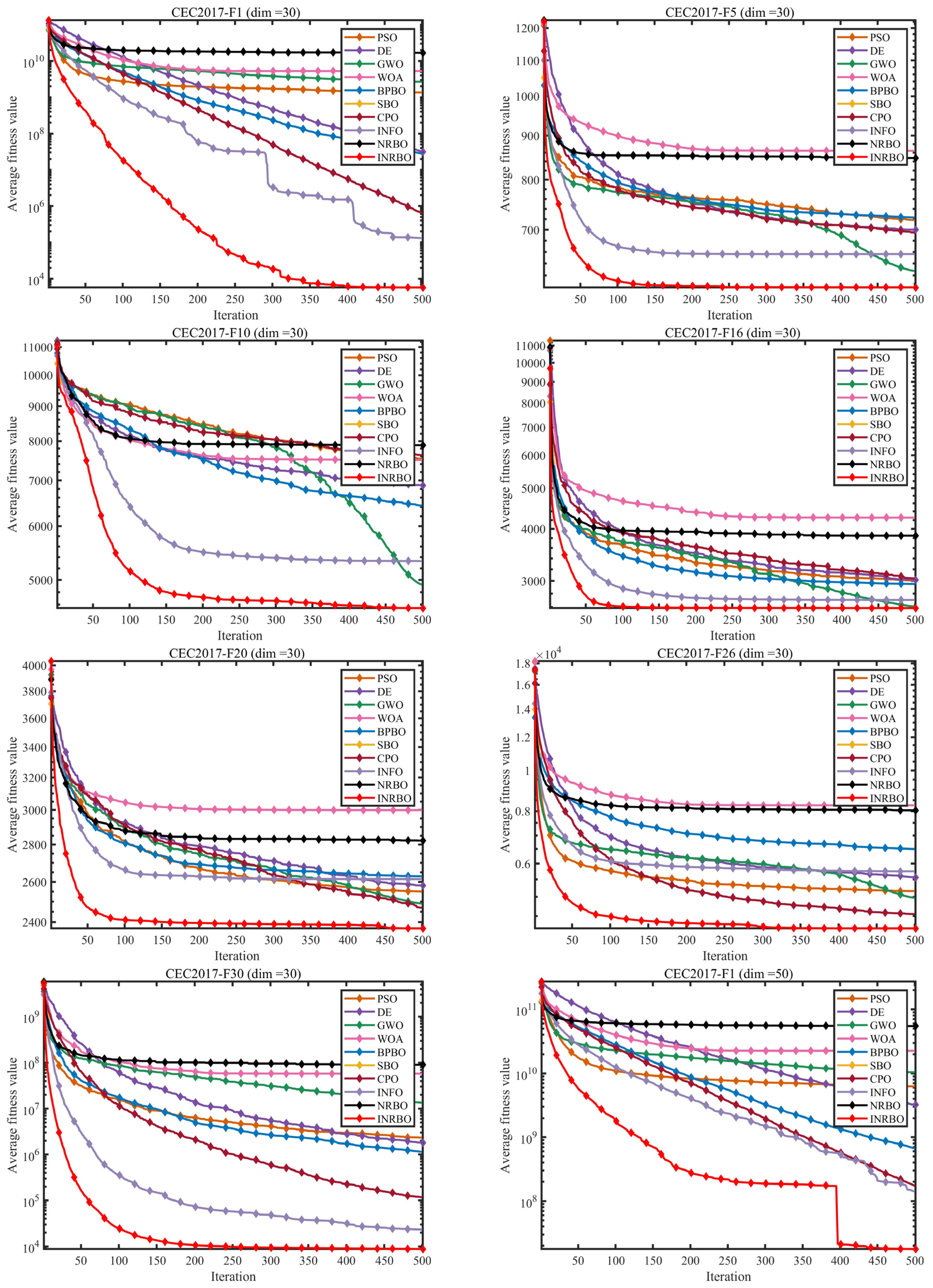
Figure 3’s convergence curves visually illustrate the optimization dynamics of all algorithms across different dimensions and function types. INRBO consistently exhibits the ideal convergence pattern of “rapid decline in early iterations, steady improvement in mid-iterations, and stable final convergence without oscillations”, and this advantage becomes more pronounced as the problem dimensionality increases.

In low-dimensional scenarios (dim = 30), INRBO’s convergence speed is evident in the early iterations: for F1, after 50 iterations, INRBO’s fitness value has already dropped to the order of 108, whereas the original NRBO remains at 1010, and PSO, DE, and other algorithms even reach 10¹¹. This demonstrates that INRBO’s early-stage convergence is two orders of magnitude faster than NRBO. After 100 iterations, INRBO further reduces the fitness to the order of 107, while NRBO is still around 109, and by 500 iterations, INRBO’s final fitness is nearly seven orders of magnitude lower than NRBO, with a smooth curve free of oscillations. This confirms that INRBO’s local exploitation strategy effectively controls step size, avoiding redundant searches. For multimodal functions such as F10, INRBO shows no significant plateau: after 150 iterations, its fitness has decreased by 40% relative to the initial value, whereas WOA and GWO have already stagnated in a plateau. By 500 iterations, INRBO’s fitness is 39.4% lower than WOA, highlighting its ability to escape local optima effectively.

In medium-dimensional scenarios (dim = 50), most algorithms experience a significant slowdown in convergence, whereas INRBO maintains high efficiency. For F5 (Rotated Rosenbrock Function), after 100 iterations, INRBO achieves a fitness value of 8.5 × 10², 19.0% lower than NRBO (1.05 × 10³). At 300 iterations, INRBO further reduces the fitness to 7.8 × 10², while NRBO remains at 1.0 × 10³, indicating that INRBO has already accomplished the majority of its optimization within the subsequent 200 iterations. By 500 iterations, INRBO reaches a final fitness of 7.3865 × 10², 34.8% lower than NRBO (1.1336 × 10³), with a convergence slope consistently steeper than other algorithms, demonstrating that its dynamic search strategy effectively tackles the challenges introduced by increased dimensionality. For the complex hybrid function F30 at dim = 50, the search space is extremely intricate. INRBO’s convergence curve maintains a stable downward trend: after 200 iterations, the fitness is 2.5 × 10⁴, 99.95% lower than NRBO (5.0 × 10⁷), and by 500 iterations, the final fitness reaches 1.0418 × 10⁶, 99.85% lower than NRBO (7.0167 × 10⁸), far outperforming all other algorithms in optimization efficiency.

In high-dimensional scenarios (dim = 100), often regarded as the “litmus test” for algorithm performance, most algorithms suffer from the curse of dimensionality, leading to premature convergence. INRBO, however, further amplifies its convergence advantage. For F1 (Sphere Function), after 100 iterations, INRBO achieves a fitness value on the order of 1.0 × 10⁹, while PSO, DE, and other algorithms have already reached 10¹¹, and NRBO is at 1.5 × 10¹¹, showing that INRBO’s early-stage convergence speed exceeds NRBO by roughly one order of magnitude. After 300 iterations, INRBO reduces the fitness to 6.5 × 10⁸, whereas NRBO remains around 1.2 × 10¹¹, widening the gap to 18 times. By 500 iterations, INRBO reaches a final fitness of 6.5414 × 10⁸, 99.6% lower than NRBO (1.7264 E + 11), with a smooth curve showing no noticeable oscillations. This demonstrates that the synergy of the adaptive differential operator and elitist population genetic strategy effectively mitigates efficiency degradation in high-dimensional spaces. For the multimodal function F19 (Rotated Hybrid Composition Function 8) at dim = 100, where local optima are densely distributed, INRBO’s convergence curve continues to decline steadily. By 250 iterations, the fitness decreases by 60% from the initial value, while INFO, CPO, and other algorithms have already plateaued. After 500 iterations, INRBO achieves a fitness of 7.5046 × 10³, which is 99.9998% lower than NRBO (3.4632 × 10⁹), highlighting its exceptional global search capability in high-dimensional, multimodal landscapes.

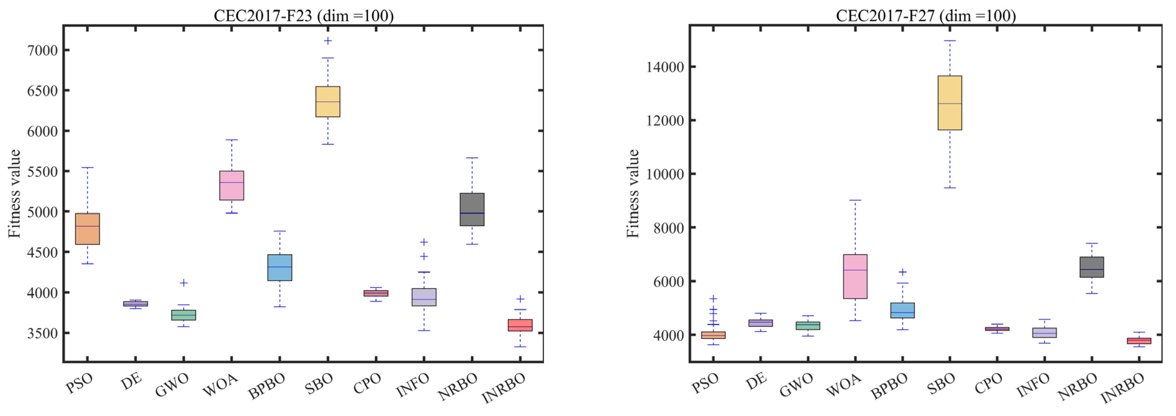
The boxplots in Figure 4 provide a statistical perspective on the performance variability of each algorithm across 30 independent runs, revealing that INRBO consistently exhibits “short boxes, short whiskers, and no outliers”, indicating its robustness under varying random initializations far surpasses the compared algorithms.

In the dim = 30 scenario, for F1 (Sphere Function), INRBO’s interquartile range (IQR) is only 1.2 E + 03, much smaller than NRBO’s 7.0 E + 09 and PSO’s 2.2 E + 09, with no outliers. This demonstrates that across 30 runs, INRBO reliably converges to high-quality solution regions. For the multimodal function F10 (Schwefel’s Function), INRBO’s median is 4.4 E + 03, 38.9% lower than WOA’s median (7.2 E + 03), and its box width is 8.0 E + 02, only 72.7% of WOA’s (1.1 E + 03), confirming that INRBO achieves high precision and excellent stability in multimodal landscapes.

In the dim = 50 scenario, for F5 (Rotated Rosenbrock Function), INRBO’s box width is 1.0 E + 02, 85.3% lower than NRBO (which shows longer whiskers), and exhibits no outliers, while NRBO has multiple outliers exceeding 1.2 E + 03, indicating that INRBO is less sensitive to random initial conditions in high-dimensional unimodal functions. For the complex hybrid function F22, INRBO’s median is 8.0 E + 03, 18.4% lower than INFO’s (9.8 E + 03), and the IQR is 4.8 E + 02, only 26.7% of INFO’s (1.8 E + 03), further validating INRBO’s robustness in high-dimensional, mixed-function optimization tasks.

In the dim = 100 scenario, most algorithms’ boxplots exhibit “wide boxes, long whiskers, and numerous outliers” (for example, the whiskers of SBO’s boxplot on F2 extend to the magnitude of 10¹⁸⁰), whereas INRBO remains stable. In the boxplot of function F1, INRBO’s interquartile range is 1.9 E + 08, far lower than NRBO’s 2.8 E + 11 and PSO’s 1.8 E + 10, with no outliers. In the boxplot of function F28, INRBO’s median is 3.8 E + 03, 34.5% lower than CPO’s median (5.8 E + 03), and its interquartile range is 3.2 E + 02, only 38.1% of CPO’s range (8.4 E + 02), demonstrating that it can maintain stable optimization performance even in high-dimensional complex functions. This stability benefits from the elite population genetic strategy, which ensures the consistent inheritance of high-quality genes, and the secondary interpolation strategy, which precisely controls the quality of local solutions, effectively reducing performance fluctuations caused by random perturbations.

Based on the quantitative metrics in Table 2, Table 3 and Table 4, the convergence curves in Figure 3, and the boxplots in Figure 4, the following key conclusions can be drawn: INRBO, through the synergistic integration of three core strategies—adaptive differential operators, secondary interpolation, and elite population genetics—comprehensively outperforms the original NRBO and other mainstream swarm intelligence algorithms in terms of optimization accuracy, convergence efficiency, and robustness. Specifically, in terms of accuracy, INRBO achieves the best Ave and Std values across all dimensions and all function types, and in high-dimensional complex functions, it reduces errors by one or more orders of magnitude compared to other algorithms. Regarding convergence efficiency, INRBO exhibits the ideal pattern of “fast in the early stage, stable in the middle stage, and no oscillation in the late stage,” with its speed advantage becoming more pronounced as dimensionality increases. In terms of robustness, INRBO’s boxplots are tightly distributed with no outliers, indicating minimal influence from random initial conditions. These performance advantages provide solid numerical support for applying INRBO to practical complex optimization problems, such as fireground robot path planning.

3.4. Experimental Results and Analysis of CEC2022

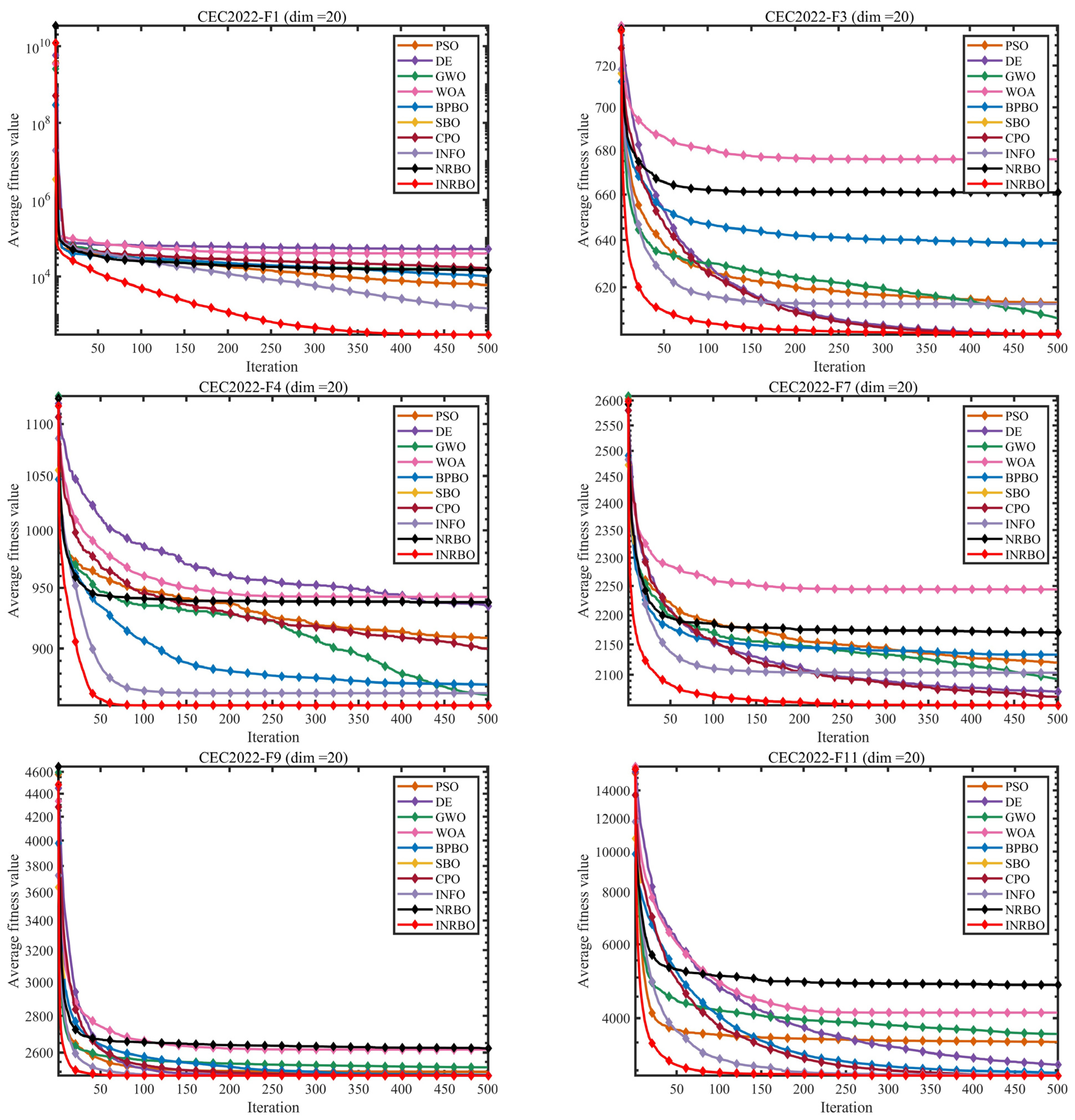
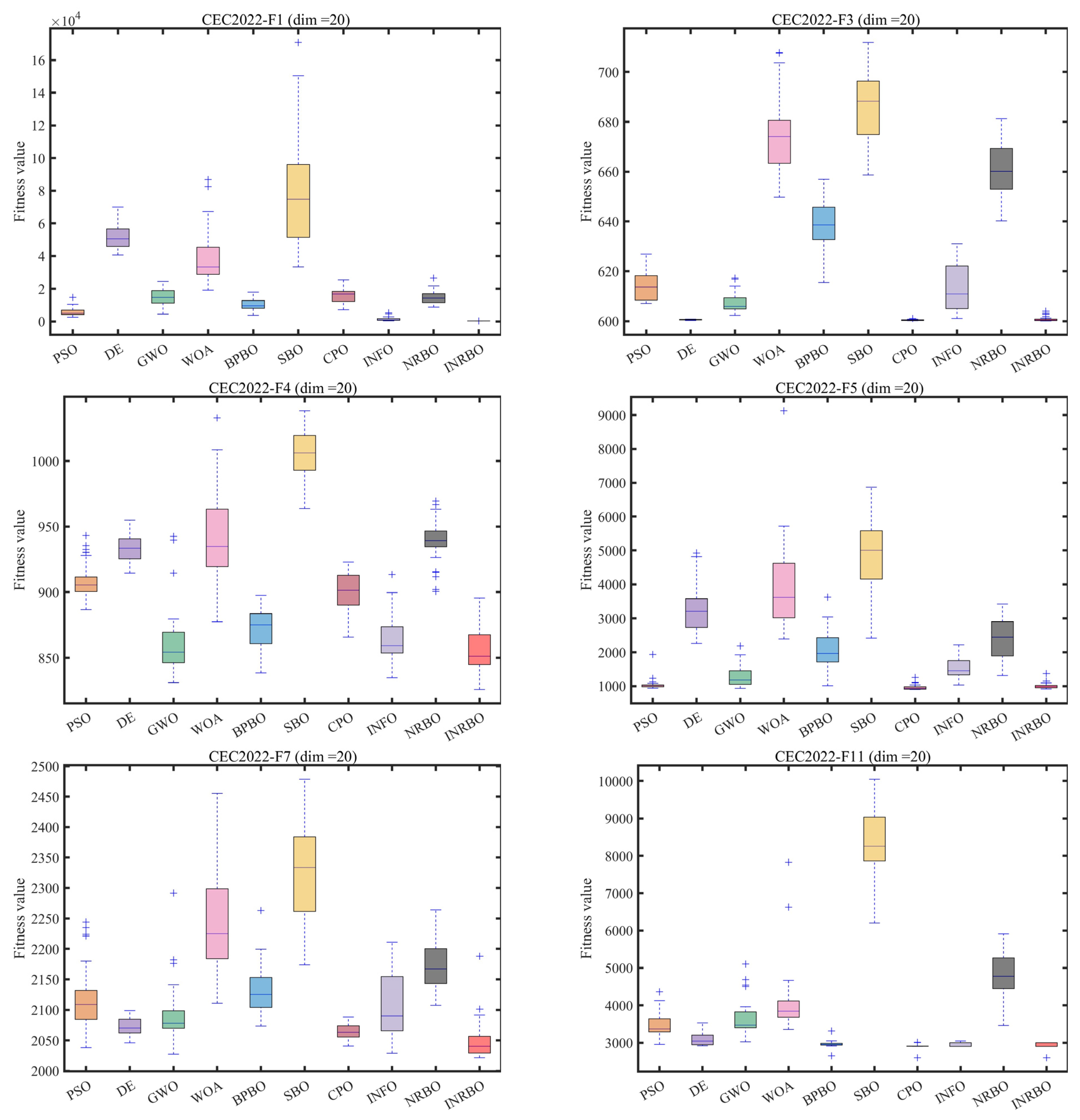
To further verify the generalization capability and stability of INRBO under different optimization scenarios, the CEC2022 benchmark test suite (dim = 20) is additionally employed for a comprehensive evaluation. This benchmark set includes unimodal, multimodal, hybrid, and composition functions, enabling a thorough assessment of the algorithm’s local search accuracy, global exploration and escape ability, and adaptability to complex search spaces. It thus forms a complementary validation framework together with CEC2017. The experimental results are presented in

Table 5. Results of CEC2022 benchmark evaluation (dim = 20).

Function	Metric	PSO	DE	GWO	WOA	BPBO	SBO	CPO	INFO	NRBO	INRBO
F1	Ave	5.9606 E + 03	5.1491 E + 04	1.5243 E + 04	3.9366 E + 04	1.0299 E + 04	7.8827 E + 04	1.6295 E + 04	1.4645 E + 03	1.4489 E + 04	3.0442 E + 02
	Std	2.7867 E + 03	7.0742 E + 03	4.9108 E + 03	1.6707 E + 04	3.3185 E + 03	3.4655 E + 04	5.0824 E + 03	1.3633 E + 03	3.8856 E + 03	6.6322 E + 00
F2	Ave	4.9379 E + 02	4.6996 E + 02	5.0409 E + 02	6.3742 E + 02	4.8056 E + 02	2.5012 E + 03	4.6452 E + 02	4.5375 E + 02	7.3949 E + 02	4.4761 E + 02
	Std	4.4486 E + 01	1.3001 E + 01	3.9114 E + 01	7.5169 E + 01	3.1173 E + 01	9.3811 E + 02	1.9811 E + 01	1.7989 E + 01	9.9923 E + 01	1.7645 E + 01
F3	Ave	6.1360 E + 02	6.0058 E + 02	6.0719 E + 02	6.7591 E + 02	6.3859 E + 02	6.8676 E + 02	6.0043 E + 02	6.1305 E + 02	6.6091 E + 02	6.0080 E + 02
	Std	5.6142 E + 00	1.5100 E − 01	3.9596 E + 00	1.4852 E + 01	1.1095 E + 01	1.3802 E + 01	2.5325 E − 01	8.9767 E + 00	1.0468 E + 01	9.6943 E − 01
F4	Ave	9.0858 E + 02	9.3462 E + 02	8.6346 E + 02	9.4221 E + 02	8.7149 E + 02	1.0061 E + 03	8.9943 E + 02	8.6474 E + 02	9.3780 E + 02	8.5540 E + 02
	Std	1.3915 E + 01	1.1105 E + 01	2.9049 E + 01	3.5178 E + 01	1.6906 E + 01	1.7581 E + 01	1.5184 E + 01	1.7096 E + 01	1.6403 E + 01	1.7550 E + 01
F5	Ave	1.0483 E + 03	3.2793 E + 03	1.2744 E + 03	3.8907 E + 03	2.0405 E + 03	4.8012 E + 03	9.5878 E + 02	1.5169 E + 03	2.4058 E + 03	1.0056 E + 03
	Std	1.7688 E + 02	6.8282 E + 02	3.2894 E + 02	1.3367 E + 03	5.9951 E + 02	1.0642 E + 03	7.8404 E + 01	2.9569 E + 02	5.4049 E + 02	8.8265 E + 01
F6	Ave	2.0682 E + 06	5.9905 E + 06	5.7149 E + 06	4.7335 E + 06	4.3404 E + 03	1.4524 E + 09	1.5568 E + 04	6.4601 E + 03	2.4570 E + 07	5.6877 E + 03
	Std	1.5152 E + 06	3.3238 E + 06	1.3820 E + 07	7.2334 E + 06	3.2699 E + 03	7.6051 E + 08	1.1791 E + 04	6.4883 E + 03	2.5160 E + 07	4.1115 E + 03
F7	Ave	2.1198 E + 03	2.0727 E + 03	2.0930 E + 03	2.2440 E + 03	2.1333 E + 03	2.3239 E + 03	2.0641 E + 03	2.1035 E + 03	2.1707 E + 03	2.0507 E + 03
	Std	5.3395 E + 01	1.3767 E + 01	5.2945 E + 01	8.3857 E + 01	4.0059 E + 01	8.0702 E + 01	1.2315 E + 01	5.1564 E + 01	3.7646 E + 01	3.3407 E + 01
F8	Ave	2.3089 E + 03	2.2301 E + 03	2.2578 E + 03	2.3168 E + 03	2.2786 E + 03	2.6482 E + 03	2.2309 E + 03	2.2731 E + 03	2.3200 E + 03	2.2262 E + 03
	Std	8.0948 E + 01	2.3003 E + 00	4.7080 E + 01	9.7241 E + 01	5.7122 E + 01	1.9670 E + 02	2.2201 E + 00	7.3650 E + 01	5.8085 E + 01	2.1713 E + 01
F9	Ave	2.4996 E + 03	2.4812 E + 03	2.5225 E + 03	2.6150 E + 03	2.4853 E + 03	3.0196 E + 03	2.4823 E + 03	2.4808 E + 03	2.6213 E + 03	2.4808 E + 03
	Std	2.7075 E + 01	4.1520 E − 01	2.9244 E + 01	4.1051 E + 01	4.5638 E + 00	1.2504 E + 02	1.0832 E + 00	3.8405 E − 05	6.2717 E + 01	6.1554 E − 07
F10	Ave	3.9434 E + 03	2.5336 E + 03	3.4922 E + 03	4.7759 E + 03	3.2745 E + 03	6.2772 E + 03	2.5625 E + 03	3.2725 E + 03	5.1389 E + 03	2.6389 E + 03
	Std	9.8727 E + 02	3.0073 E + 01	7.3721 E + 02	1.3530 E + 03	1.0444 E + 03	1.9717 E + 03	1.1031 E + 02	5.9121 E + 02	1.6166 E + 03	1.6029 E + 02
F11	Ave	3.5098 E + 03	3.0955 E + 03	3.6647 E + 03	4.1214 E + 03	2.9635 E + 03	8.4011 E + 03	2.9170 E + 03	2.9289 E + 03	4.8007 E + 03	2.9167 E + 03
	Std	3.3121 E + 02	1.7360 E + 02	4.7550 E + 02	9.1632 E + 02	9.4004 E + 01	8.6793 E + 02	7.3439 E + 01	4.8019 E + 01	5.5509 E + 02	9.8553 E + 01
F12	Ave	3.0069 E + 03	2.9510 E + 03	2.9791 E + 03	3.1273 E + 03	3.0179 E + 03	3.4453 E + 03	2.9840 E + 03	2.9742 E + 03	3.0425 E + 03	2.9716 E + 03
	Std	5.8984 E + 01	4.1490 E + 00	1.9133 E + 01	1.2998 E + 02	4.7577 E + 01	1.5925 E + 02	1.2938 E + 01	2.9925 E + 01	7.2975 E + 01	4.9112 E + 01

, Figure 5 and Figure 6.

Table 5 presents the performance results of INRBO compared with nine other mainstream algorithms on the CEC2022 benchmark test suite (dim = 20). The results demonstrate that INRBO exhibits significant advantages across multiple categories of benchmark functions. For the unimodal function F1, the mean fitness value achieved by INRBO (3.0442 E + 02) is only 20.8% of that obtained by the second-best algorithm, INFO (1.4645 E + 03), while its standard deviation (6.6322 E + 00) is as low as 0.49% of that of INFO, indicating exceptionally high local search accuracy and stability. For the complex multimodal function F6, INRBO achieves a mean fitness value of 5.6877 E + 03, substantially outperforming all other algorithms and reducing the value by 99.97% compared with the original NRBO (2.4570 E + 07), effectively avoiding local optimum traps. Even for the high-dimensional and challenging F5 function, INRBO maintains a mean fitness value of 1.0056 E + 03, second only to CPO (9.5878 E + 02), while its standard deviation (8.8265 E + 01) is merely 16.3% of that of NRBO (5.4049 E + 02), demonstrating excellent robustness.

The convergence curves shown in Figure 5 visually illustrate the optimization dynamics of the compared algorithms. INRBO consistently exhibits the ideal behavior of “rapid early decline, steady mid-stage improvement, and oscillation-free convergence in the later stage.” Taking function F1 as an example, INRBO reduces the fitness value to below the 10⁵ level within 100 iterations, whereas NRBO, PSO, and other algorithms require more than 300 iterations to reach a comparable level, achieving a convergence speed improvement of more than twofold. For function F9, the convergence curve of INRBO shows no obvious stagnation throughout the entire process, and its final fitness value is 17.7% lower than that of SBO, fully demonstrating its ability to dynamically balance global exploration and local exploitation.

The box plots in Figure 6 further confirm the stability of INRBO. Both the box height and whisker length are significantly smaller than those of the other algorithms, and no outliers are observed for functions such as F4 and F7. This indicates that even under different random initialization conditions, INRBO can consistently produce high-quality solutions, providing reliable assurance for practical engineering applications.

Overall, the performance of INRBO on the CEC2022 benchmark is highly consistent with its results on CEC2017. Through the synergistic integration of adaptive differential operators, quadratic interpolation, and elite genetic strategies, INRBO achieves simultaneous improvements in optimization accuracy, convergence speed, and robustness across unimodal, multimodal, and complex hybrid functions. Compared with traditional algorithms, INRBO demonstrates stronger adaptability to different types of optimization problems, and its performance advantages are particularly pronounced in low-dimensional yet highly complex scenarios, laying a solid algorithmic foundation for subsequent engineering applications such as mobile robot path planning.

3.5. Analysis of Population Diversity

In evolutionary and swarm-based optimization methods, population diversity reflects the extent of differences among individuals within a population [29,38], where each individual represents a potential solution. Insufficient diversity often causes the algorithm to converge prematurely to suboptimal solutions, thereby weakening its ability to perform an effective global search. Conversely, maintaining a diverse population encourages extensive exploration of the search space and increases the likelihood of identifying the global optimum. In this subsection, the diversity performance of the MECOA algorithm is quantitatively analyzed using Equation (13).

$$I_C\left(t\right)=\sqrt{\sum _{i=1}^N \sum _{d=1}^D {\left(x_{id}\left(t\right)-c_d\left(t\right)\right)}^2}$$

(21)

where $I_C\left(t\right)$ represents the population diversity at iteration $t$, $N$ is the number of individuals in the population, and $D$ denotes the dimensionality of the optimization problem. The term $x_{id}\left(t\right)$ refers to the position of the $i$-th individual in the $d$-th dimension at iteration $t$. The parameter $c_d\left(t\right)$ indicates the coordinate of the population’s centroid in the $d$-th dimension at iteration $t$, which is computed as follows:

$$c_d\left(t\right)={\displaystyle \frac{1}{D}}\sum _{i=1}^N x_{id}\left(t\right)$$

(22)

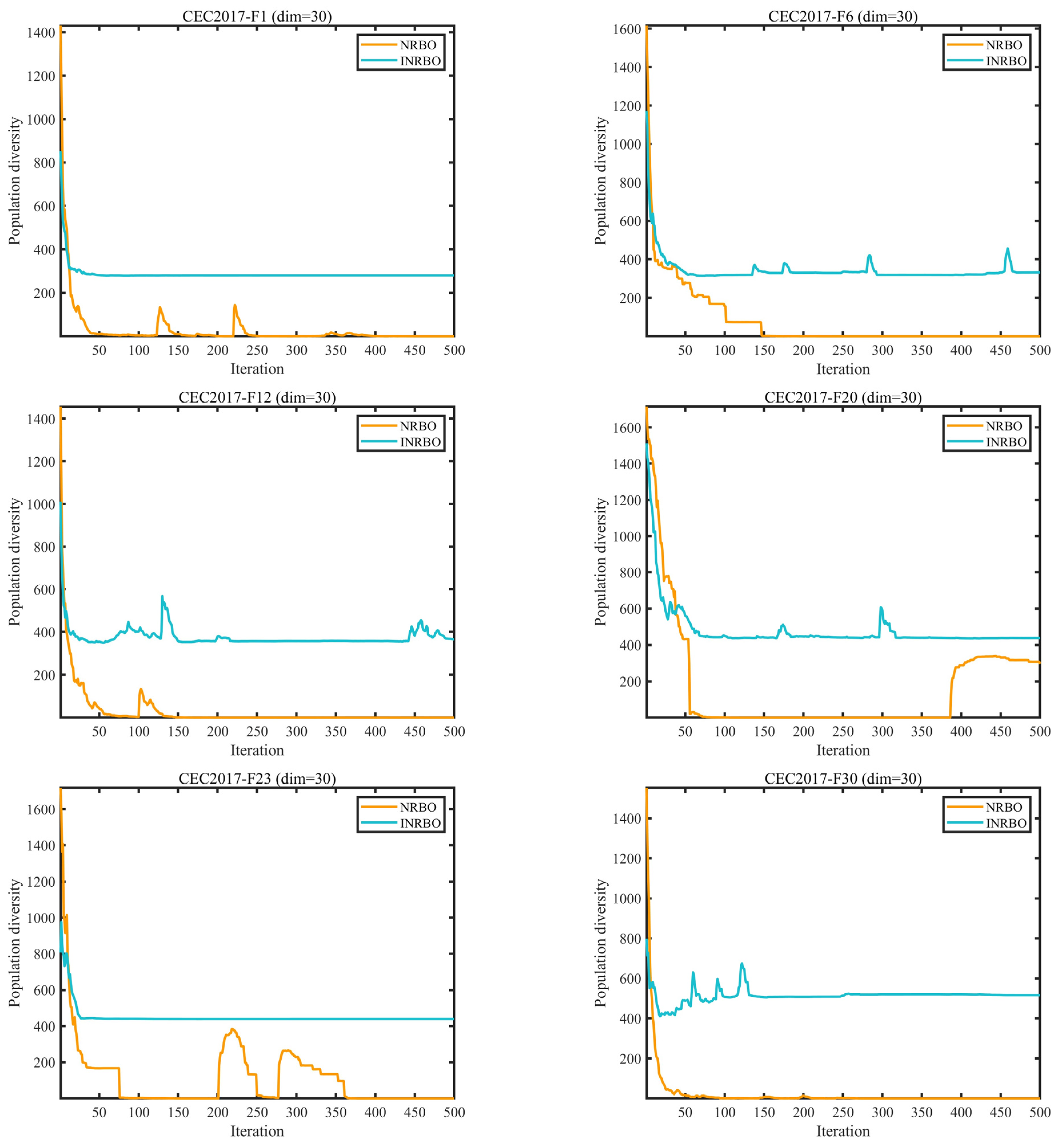
Population diversity is a key factor influencing the global exploration capability of optimization algorithms and their ability to avoid premature convergence. Figure 7 compares the population diversity curves of INRBO and the original NRBO on different functions of the CEC2017 benchmark suite (dim = 30), visually demonstrating the dynamic population advantages of INRBO. Overall, the diversity curve of INRBO remains within a reasonable fluctuation range throughout the optimization process, avoiding both excessive diversity that may lead to disordered search and overly rapid diversity loss that can cause local stagnation, thereby achieving a dynamic balance between exploration and convergence.

For the unimodal function F1, the population diversity of NRBO decreases rapidly in the early iterations and stabilizes at a low level after about 200 iterations, indicating premature homogenization of the population and limited capability for further precision improvement through local refinement. In contrast, INRBO maintains a relatively high diversity level in the early stage, providing sufficient space for global exploration, and then gradually decreases after around 300 iterations, ensuring a smooth transition toward local exploitation in the later stage. This behavior is consistent with the previously observed high-precision performance of INRBO on unimodal functions.

For the multimodal function F12, the diversity curve of NRBO exhibits large fluctuations and remains at an overall low level, reflecting its tendency to become trapped in local optima within landscapes containing multiple local minima. INRBO, however, preserves a more stable and higher diversity level, particularly during the critical iteration interval from 150 to 300, where no sharp decline in diversity is observed. This enables sustained exploration of new regions in the search space and effective avoidance of local optimum traps.

In the composition function F30, NRBO shows an unstable “sharp rise and sharp fall” pattern in its diversity curve, indicating insufficient adaptability of its population update mechanism to complex search spaces and a tendency toward population divergence or stagnation. By contrast, the diversity curve of INRBO remains smoothly fluctuating and consistently within a reasonable range throughout the entire iteration process. This stability can be attributed to the elite genetic strategy, which preserves high-quality genetic information while introducing moderate variation, and to the adaptive differential operator, which dynamically adjusts search step sizes. Together, these mechanisms allow the population to inherit superior traits while maintaining sufficient diversity.

In summary, through the synergistic effects of its three core strategies, INRBO achieves precise regulation of population diversity, providing a critical foundation for its superior performance across different types of benchmark functions.

3.6. Compare Experimental Results Using the Maximum Number of Evaluations

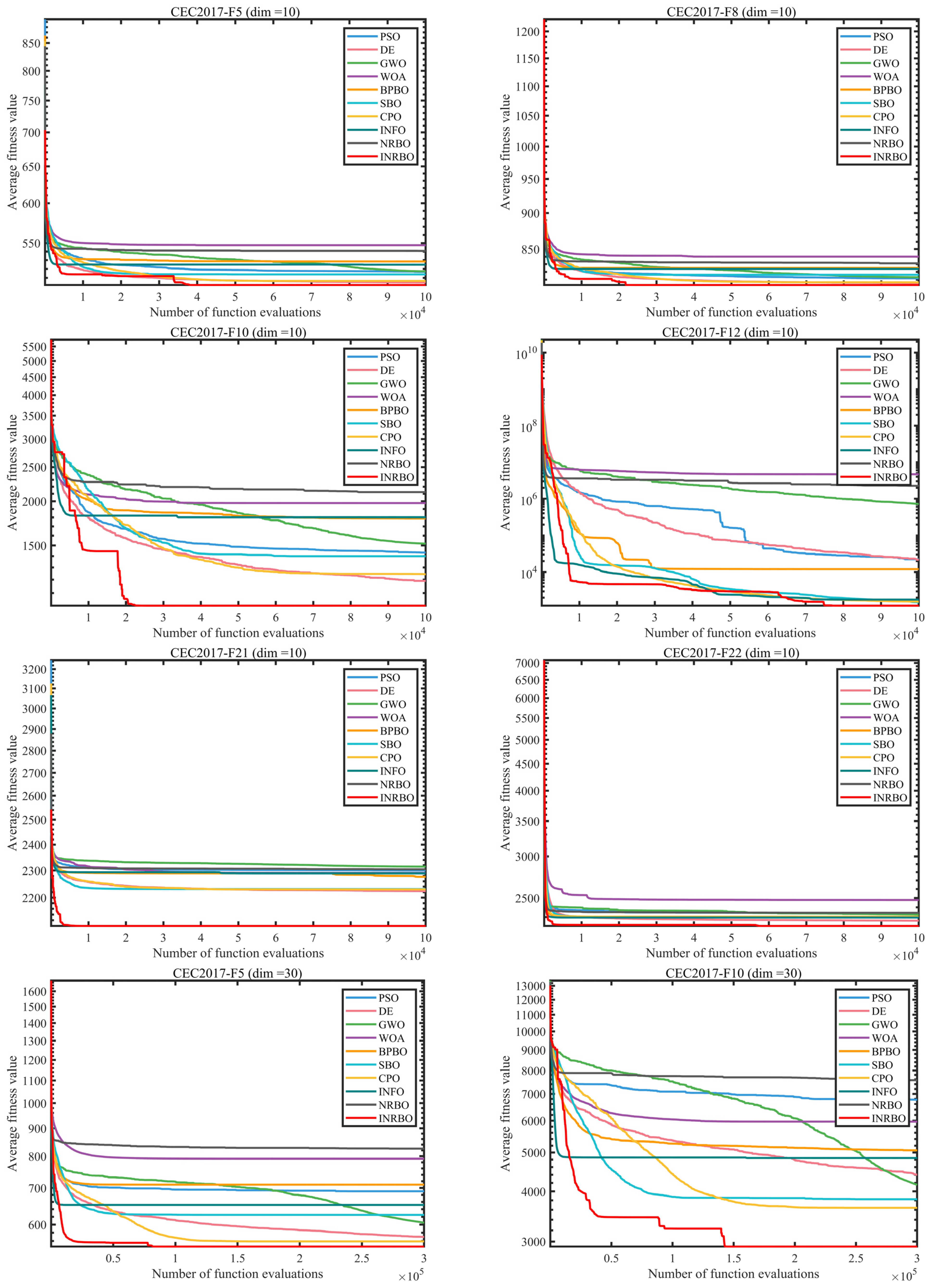
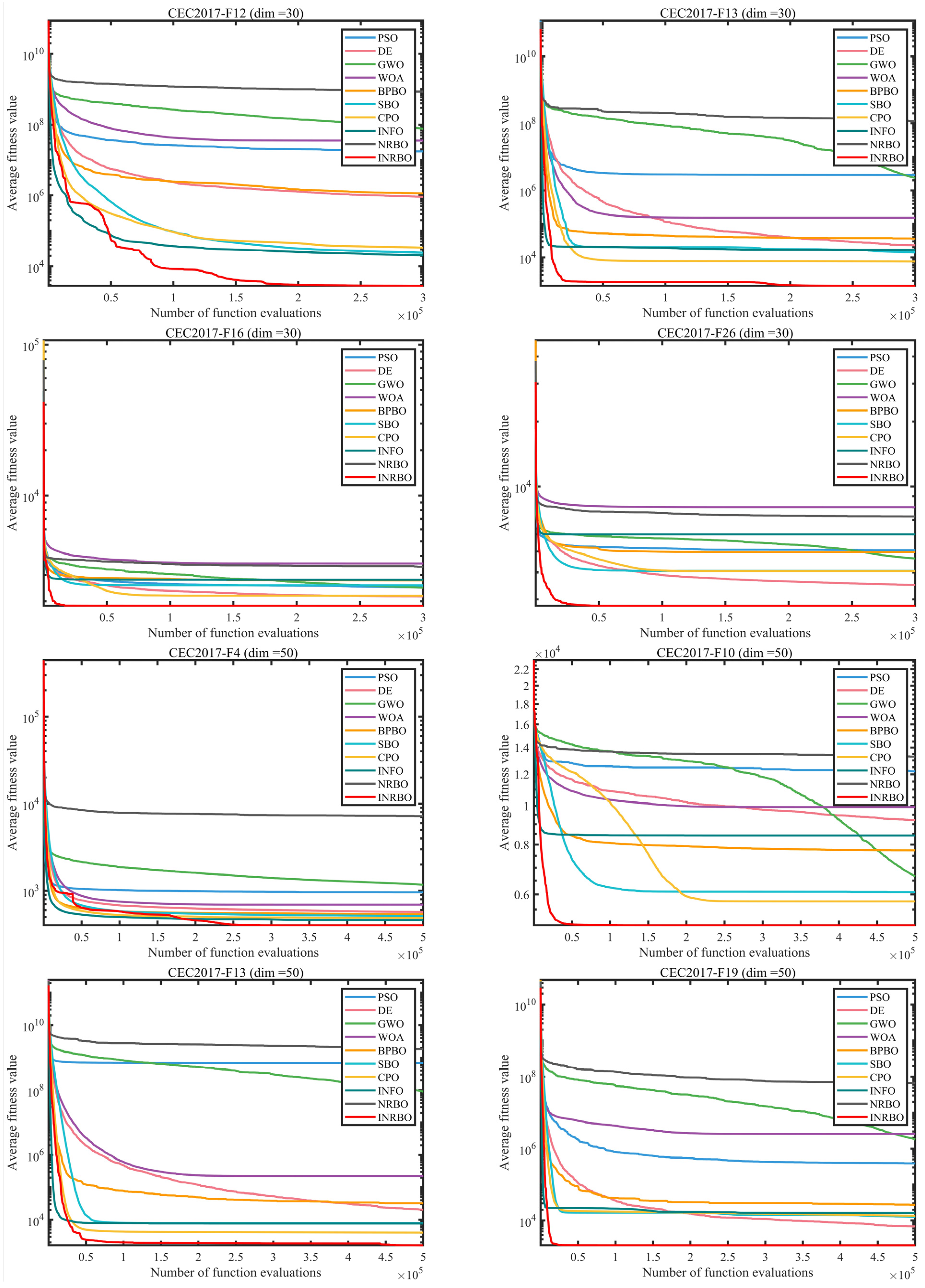
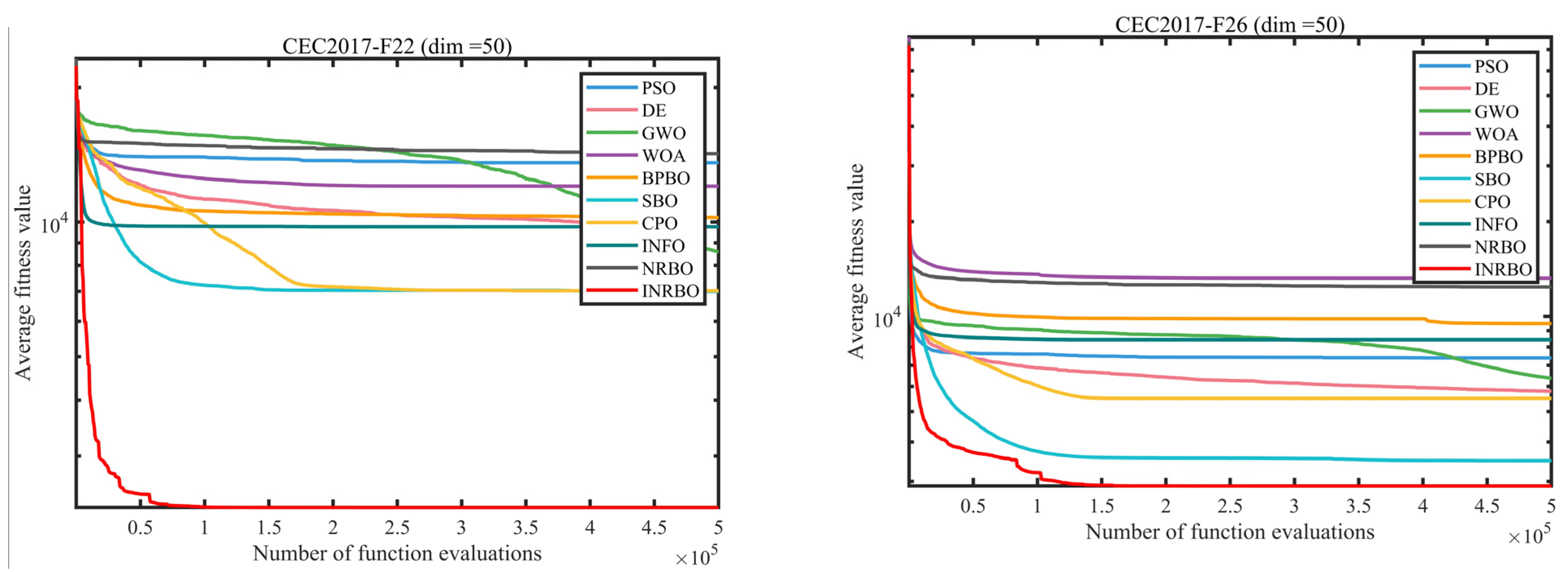
To ensure a fair comparison of metaheuristic algorithms, this section uses $MaxFES$ to evaluate their effectiveness. In our experiments, we set the population size to 30 and the maximum number of evaluations to $\mathrm{10,000} \ast dim$. The remaining parameters of the algorithm are set the same as in Section 3.1. We conducted comprehensive experiments on the CEC2017 test set in 10, 30, and 50 dimensions. The convergence curves of all compared algorithms are shown in Figure 8.

Figure 8 compares the convergence curves of different algorithms on the CEC2017 test set under 10, 30, and 50-dimensional conditions, with all algorithms running under the same function evaluation number constraint (MaxFES = 10,000 × dim) and consistent parameter settings. It can be observed that INRBO exhibits faster convergence speed and lower final fitness value on most test functions: its convergence curve declines more steeply in the early stages, indicating that the algorithm can perform global search more efficiently and quickly approach high-quality solutions; in the mid-to-late stages, INRBO continues to improve the quality of solutions, while the comparative algorithms (including the original NRBO) often enter a state of convergence stagnation or slowing decline earlier. As the problem dimension increases, the convergence performance of other algorithms is generally significantly affected, while INRBO maintains stable and competitive convergence behavior, indicating that it has stronger robustness and search efficiency in high-dimensional complex search spaces. In summary, the experimental results in Figure 8 verify that INRBO can achieve faster convergence speed and better final solution quality under the same computational budget, demonstrating its effectiveness in balancing exploration and development.

3.7. Statistical Analysis

3.7.1. Friedman Mean Rank Test

To build a complete evaluation framework for the INRBO method, statistical tools that can evaluate several interrelated algorithms simultaneously are required. Designed especially for this objective, the Friedman test provides a non-parametric technique comparing different methods according to their ranked results over diverse datasets. It naturally avoids any presuppositions about the actual distribution of measured outcomes. This characteristic makes it highly effective for comparing multiple approaches tested on the same collection of benchmark tasks. The computation of the Friedman metric adheres to the expression below [39,40]:

$$Q={\displaystyle \frac{12}{kn\left(k+1\right)}}\sum _{j=1}^k{R}_j^2-3n\left(k+1\right)$$

(23)

In this formula, $n$ indicates how many blocks are present, $k$ stands for the total treatment groups, and $R_j$ reflects the aggregated rank score of the $j^{th}$ group. When the sample sizes of $n$ and $k$ are both large enough, the resulting metric $Q$ can be closely approximated using a ${\chi }^2$ distribution with $k-1$ degrees of freedom [38].

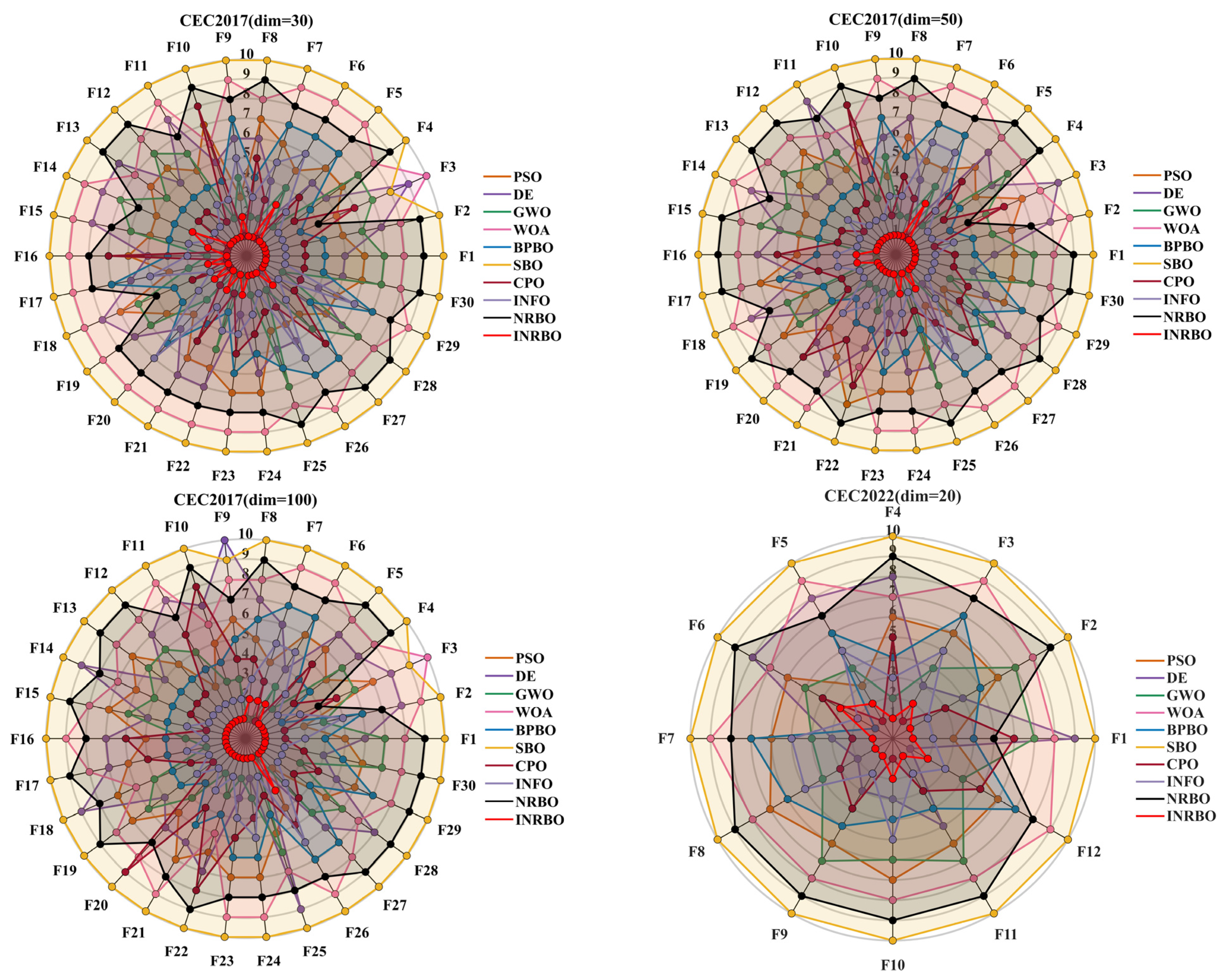
The average ranking results of the Friedman test (

Table 6. Mean ranks from the Friedman test for all compared methods.

Suites	CEC2017						CEC2022
Dimensions	30		50		100		20
Algorithms	$\mathit{M}.\mathit{R}$	$\mathit{T}.\mathit{R}$	$\mathit{M}.\mathit{R}$	$\mathit{T}.\mathit{R}$	$\mathit{M}.\mathit{R}$	$\mathit{T}.\mathit{R}$	$\mathit{M}.\mathit{R}$	$\mathit{T}.\mathit{R}$
PSO	5.43	6	5.60	6	5.50	6	5.67	7
DE	5.70	7	5.77	7	6.33	7	4.75	4
GWO	4.43	4	4.23	4	4.07	3	5.08	6
WOA	8.57	9	8.30	9	8.03	8	8.17	8
BPBO	4.97	5	4.80	5	4.77	5	5.00	5
SBO	9.93	10	10.00	10	9.93	10	10.00	10
CPO	3.27	2	3.93	3	4.07	3	3.17	2
INFO	3.33	3	2.90	2	2.90	2	3.42	3
NRBO	8.00	8	8.27	8	8.23	9	8.25	9
INRBO	1.37	1	1.20	1	1.17	1	1.50	1

) comprehensively verify the statistical superiority of INRBO across different benchmark test suites and dimensional settings. On the CEC2017 test suite, as the dimensionality increases from 30 to 100, INRBO consistently maintains the first average rank, with the performance gap relative to other algorithms continuously widening. Specifically, its average rank is 1.37 at 30 dimensions, improves to 1.20 at 50 dimensions, and is further optimized to 1.17 at 100 dimensions, demonstrating strong adaptability in high-dimensional optimization scenarios.

On the CEC2022 test suite (20 dimensions), INRBO also ranks first with an average rank of 1.50, significantly outperforming the second-ranked CPO (3.17) and the third-ranked INFO (3.42), confirming that its performance advantage is consistent across different test suites. In contrast, the original NRBO ranks in the lower-middle range (7th–9th) across all scenarios, while mainstream algorithms such as PSO, DE, and WOA generally achieve average ranks between 4th and 8th, making it difficult to challenge the leading position of INRBO.

The ranking distribution heatmap in Figure 9 intuitively illustrates the performance differences in the algorithms across different test functions. INRBO is highlighted with darker colors across all function types in CEC2017 (30/50/100 dimensions) and CEC2022 (20 dimensions), indicating that it can consistently produce optimal or near-optimal solutions on unimodal, multimodal, hybrid, and composite functions, without any evident performance weaknesses.

In contrast, other algorithms exhibit pronounced function dependency. For example, WOA performs reasonably well on some low-dimensional multimodal functions, but its ranking drops sharply in high-dimensional scenarios. Although CPO and INFO can reach the top three on certain functions, they struggle to maintain their advantages on complex composite functions. This distributional disparity further confirms that, through the synergistic effect of its three core strategies, INRBO achieves a dynamic balance between exploration and exploitation, resulting in significantly superior performance stability and generalization capability compared with the benchmark algorithms.

3.7.2. Wilcoxon Rank-Sum Test

In this subsection, the Wilcoxon rank-sum test is employed to examine whether statistically significant differences exist in the performance of the INRBO algorithm, without relying on the assumption of data normality. Compared with the traditional t-test, the Wilcoxon test is more flexible and robust, as it is applicable to data with non-normal distributions and is less sensitive to outliers [39]. The statistical results are summarized in

Table 7. Results for various algorithms on the CEC2017 and CEC2022.

Statistical Results	CEC2017 dim = 30 (+/=/−)	CEC2017 dim = 50 (+/=/−)	CEC20100 dim = 30 (+/=/−)	CEC2022 dim = 20 (+/=/−)
PSO	(29/0/1)	(29/0/1)	(29/0/1)	(11/0/1)
DE	(29/0/1)	(30/0/0)	(29/0/1)	(9/0/3)
GWO	(21/0/9)	(21/0/9)	(23/0/7)	(11/0/1)
WOA	(30/0/0)	(30/0/0)	(30/0/0)	(12/0/0)
BPBO	(30/0/0)	(30/0/0)	(30/0/0)	(10/0/2)
SBO	(30/0/0)	(30/0/0)	(30/0/0)	(12/0/0)
CPO	(27/0/3)	(30/0/0)	(29/0/1)	(10/0/0)
INFO	(24/0/6)	(28/0/2)	(30/0/0)	(9/0/3)
NRBO	30/0/0)	(30/0/0)	(30/0/0)	(12/0/0)

.

To further verify the statistical significance of the performance differences between INRBO and the other comparison algorithms, the Wilcoxon rank-sum test was employed for nonparametric statistical analysis. This method does not require the assumption of normal data distribution, is more robust to outliers, and can more objectively reflect the true performance differences among algorithms [39]. The test results are reported in the form of “+/−/=“, where “+” indicates that INRBO performs significantly better, “−” indicates that INRBO performs significantly worse, and “=“ indicates no significant difference.

As shown in Table 7, INRBO demonstrates overwhelming statistical superiority across all test scenarios. In the CEC2017 30-dimensional setting, INRBO significantly outperforms PSO on 29 out of 30 test functions, with no significant difference on only one function, and achieves full dominance (30/30 functions) over WOA, BPBO, SBO, and NRBO. In the 50-dimensional scenario, INRBO shows significant superiority over DE, WOA, BPBO, SBO, and NRBO on all functions, and also outperforms INFO on 28 functions, with no significant difference on only two functions. When the dimensionality increases to 100, INRBO maintains strong performance, with the proportion of functions showing significant superiority over all comparison algorithms exceeding 96%, and complete dominance over WOA, BPBO, SBO, and NRBO. In the CEC2022 20-dimensional scenario, INRBO again achieves full significant superiority over WOA, SBO, and NRBO on all 12 functions, and shows no significant difference on only one function each when compared with PSO and GWO, further confirming the cross-test-suite consistency of its performance advantage.

Notably, even when compared with relatively strong competitors such as CPO and INFO, the significant advantage of INRBO remains unshaken. In the CEC2017 30-dimensional setting, INRBO significantly outperforms CPO on 27 functions, with no significant difference on only three functions; compared with INFO, INRBO shows superior performance on 24 functions, with no significant difference on six functions. As the dimensionality increases, this advantage becomes even more pronounced. In the 100-dimensional setting, INRBO achieves significant superiority over INFO on all functions, fully demonstrating its statistical dominance in high-dimensional and complex optimization problems. These results indicate that the performance improvement of INRBO is not due to random factors, but rather stems from the systematic advantages of its algorithmic design, providing strong statistical support for subsequent engineering applications.

4. Mobile Robot Path Planning in Different Environments

4.1. Environment Map Modeling

Current mainstream environment modeling methods mainly include five approaches: grid maps, topological maps, semi-parametric maps, probabilistic maps, and free-space methods [41]. Topological maps excel at representing connectivity within an environment but are limited in capturing local details in continuous spaces. Probabilistic maps can better accommodate uncertain information but often incur higher computational costs. Semi-parametric and free-space methods perform well in open scenarios but struggle to adapt to densely obstructed areas or complex hazardous regions [42,43]. Considering the nonlinear characteristics of the environment, real-time operational requirements, and practical feasibility of algorithm implementation, this study selects the grid map method as the foundational approach for environment modeling.

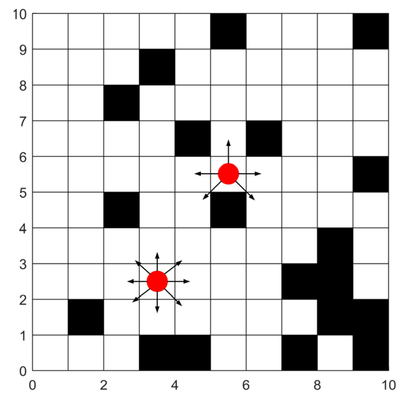
Within this modeling framework, the environment is discretized into a two-dimensional grid matrix, with each cell corresponding to a fixed region in the real-world scene. A binary encoding scheme is used to identify regions with different attributes: black grids represent obstacles or hazardous areas, indicating locations that the robot cannot traverse, while white grids represent safe areas, corresponding to regions where the robot can move freely. Robot movement follows the eight-neighborhood rule, allowing it to move one grid per step horizontally, vertically, or diagonally, while strictly avoiding obstacle cells during path search to ensure path safety and feasibility. This mechanism fully considers the robot’s need for flexible obstacle avoidance, making the generated paths more realistic and applicable to actual motion scenarios.

Through the above modeling process, environmental information is effectively transformed into a structured digital representation, providing a standardized input interface for subsequent path planning algorithms. This model supports global path search in static environments and can be extended to real-time re-planning tasks in dynamic settings, laying an important foundation for mobile robots to achieve safe and autonomous navigation in complex scenarios.

Figure 10 illustrates the robot’s mobility within the grid map. In the figure, red dots represent the robots, and arrows indicate the directions in which the robots can move. For the robot on the right, there are no surrounding obstacles, so all eight directions are traversable. For the robot on the left, obstacles exist directly above and at the upper-left position, leaving only the remaining five directions available for movement.

4.2. Experimental Analysis of Mobile Robot Path Planning in Different Environments

To evaluate the performance of INRBO in executing path planning tasks for mobile robots within complex grid environments, experiments were conducted in three grid scenarios of different scales: 20 × 20, 40 × 40, and 60 × 60. INRBO was compared with nine other algorithms—PSO, DE, GWO, WOA, BPBO, SBO, CPO, INFO, and the original NRBO—through simulation. To minimize the impact of randomness on the results, all algorithms were independently executed 30 times under identical conditions. Other parameter settings were consistent with those described in Section 3.1. In the reported tables, the “Average” represents the mean path length over the 30 runs for each algorithm; the “Maximum” and “Minimum” indicate the longest and shortest path lengths, respectively, with the optimal values among the three metrics highlighted in bold.

4.2.1. Experimental Analysis in the 20 × 20 Grid Environment

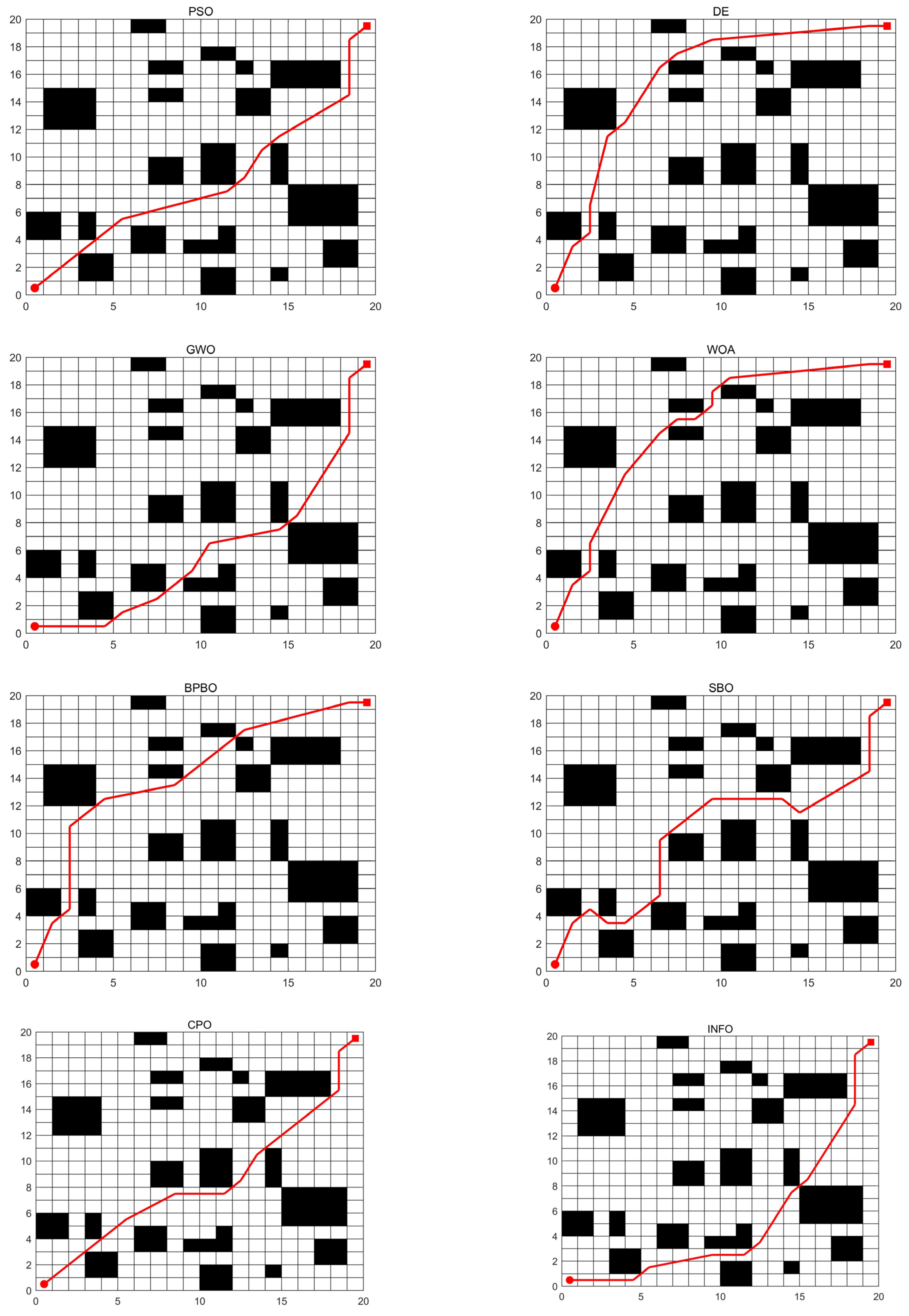
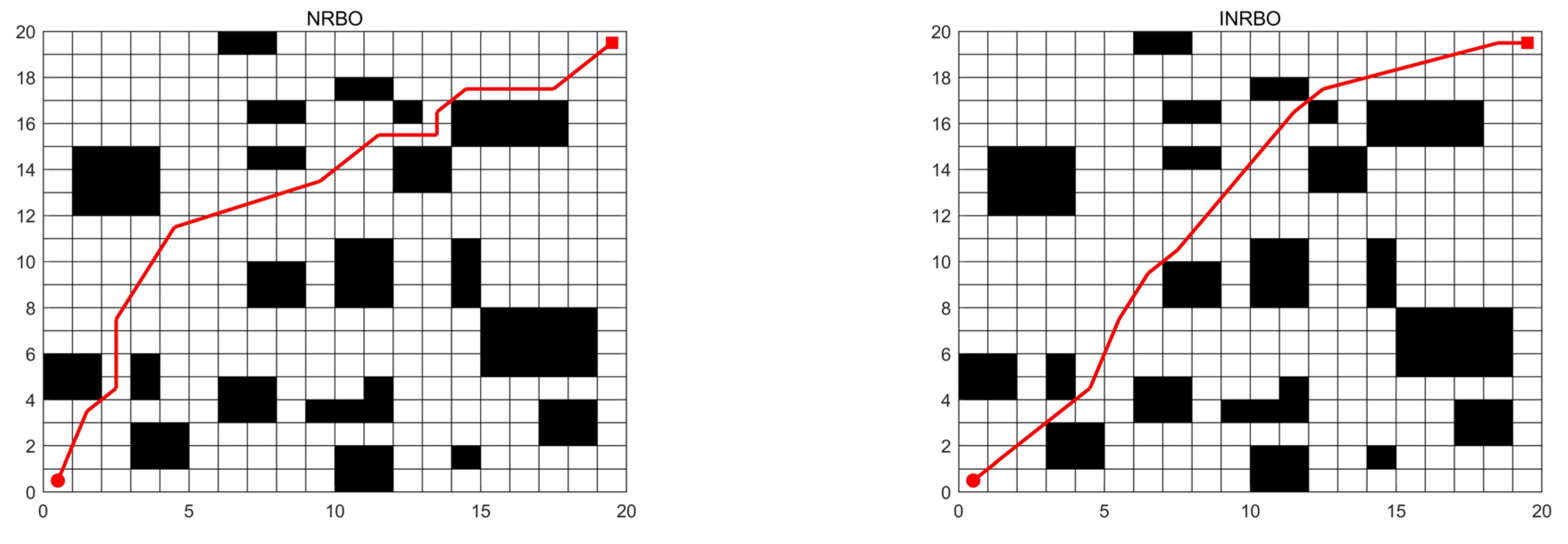
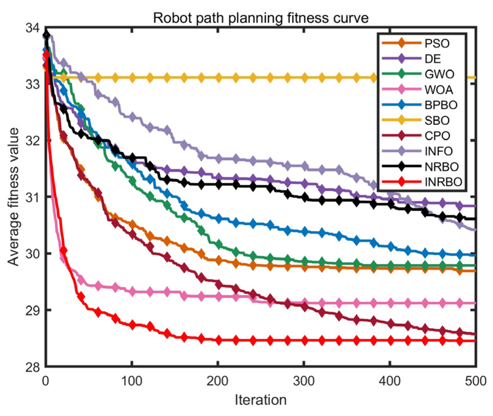
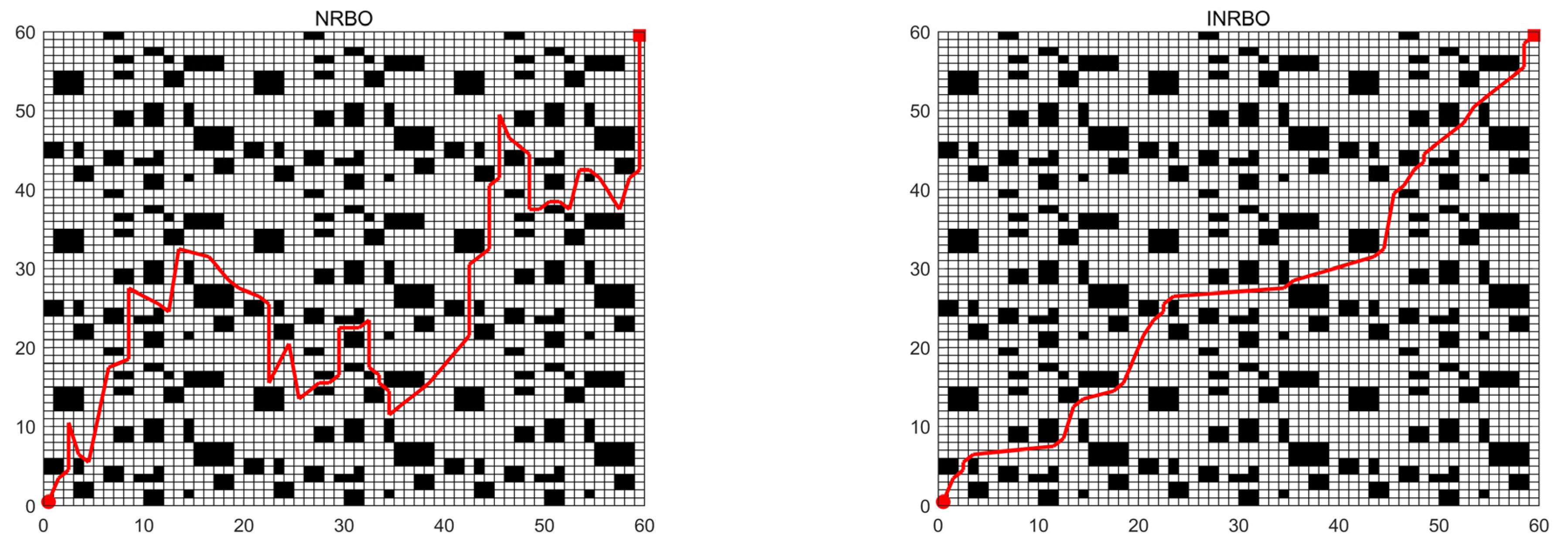
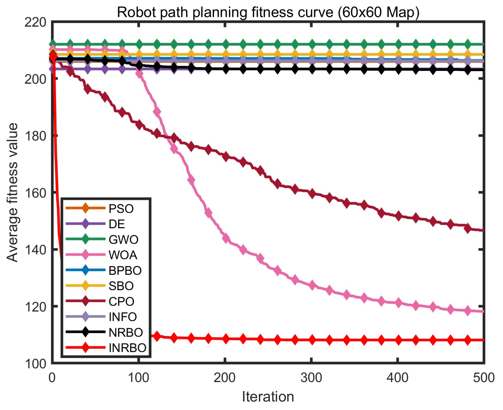
In the 20 × 20 grid environment, the starting coordinate was set at (1, 1) and the target point at (20, 20). Simulations were conducted using INRBO and the nine other comparative algorithms. The resulting planned paths are shown in Figure 11, the convergence curves are recorded in Figure 12, and the detailed comparison of performance metrics for all algorithms is summarized in

Table 8. Quantitative path planning outcomes across algorithms in a 20 × 20 grid setting (Bold formatting indicates the best values).

Algorithm	Ave	Std	Max	Min	Rank
PSO	29.6902	0.7499	31.6264	28.4193	4
DE	30.8370	0.6616	32.2887	29.183	9
GWO	29.7856	1.0732	32.1344	28.4193	5
WOA	29.1205	1.0681	31.6208	28.0192	3
BPBO	29.9642	1.1095	32.1959	28.5583	6
SBO	33.1088	1.2896	35.6803	30.2729	10
CPO	28.5694	0.2030	28.8593	28.0844	2
INFO	30.4049	0.7816	32.5471	29.0815	7
NRBO	30.5877	1.0495	32.5273	28.7715	8
INRBO	28.4531	0.3358	28.7765	27.8410	1

.

From the perspective of path characteristics (Figure 11), the paths planned by INRBO demonstrate the core advantages of “short path–high smoothness–strong obstacle avoidance.” Compared with the redundant turns in PSO paths and the obstacle detours in SBO paths, INRBO generates trajectories that extend from the start point (1,1) to the target (20,20) along the optimal direction, with no unnecessary deviations, while maintaining a safe distance from obstacle grids, fully adhering to the robot’s eight-neighborhood movement rules. Compared with the local oscillations in the original NRBO paths, INRBO trajectories are more regular, effectively reducing the robot’s motion energy consumption and control complexity. Although algorithms like CPO and WOA can generate relatively short paths, they still encounter issues such as proximity to obstacles (e.g., CPO path near grid (12,15) is only one grid away from an obstacle) or sudden directional changes (e.g., WOA path exhibits a 90° turn at (8,10)), which may increase collision risk in practical applications.

The convergence efficiency and optimization dynamics further highlight INRBO’s superiority (Figure 12). INRBO’s fitness curve rapidly decreases from 33 to below 30 within the first 100 iterations, achieving approximately 40% faster convergence than the second-ranked CPO. After 200 iterations, its fitness stabilizes around 28.5, entering the fine-tuning phase with no obvious plateau or oscillation. In contrast, NRBO, INFO, and other algorithms remain above 30 with significant fluctuations (e.g., NRBO’s fitness varies by 1.2 between 300 and 400 iterations). This behavior stems from INRBO’s adaptive differential operator and secondary interpolation strategy: the former enables rapid early-stage exploration through dynamic scaling factors, while the latter leverages high-quality solution information to guide optimal path search. Their synergy avoids the traditional algorithmic shortcomings of “insufficient exploration” or “over-exploitation.”

Quantitative metrics (Table 8) further confirm INRBO’s overwhelming performance. Its average path length (28.4531) is 6.97% shorter than the original NRBO (30.5877) and 0.41% shorter than CPO (28.5694), making it the only algorithm with an average path length below 28.5. The shortest path length (27.8410) surpasses the lower bound of all comparative algorithms, 0.64% shorter than WOA (28.0192). The standard deviation (0.3358) is only 31.3% of GWO’s (1.0732) and 30.2% of BPBO’s (1.1095). The maximum path length (28.7765) differs from the minimum by only 0.9355, demonstrating remarkable stability. In the comprehensive ranking, INRBO occupies the first position by a clear margin. Its synergistic optimization in path length, smoothness, convergence speed, and stability provides a reliable solution for efficient and safe navigation of mobile robots in small-scale complex environments.

4.2.2. Experimental Analysis in the 40 × 40 Grid Environment

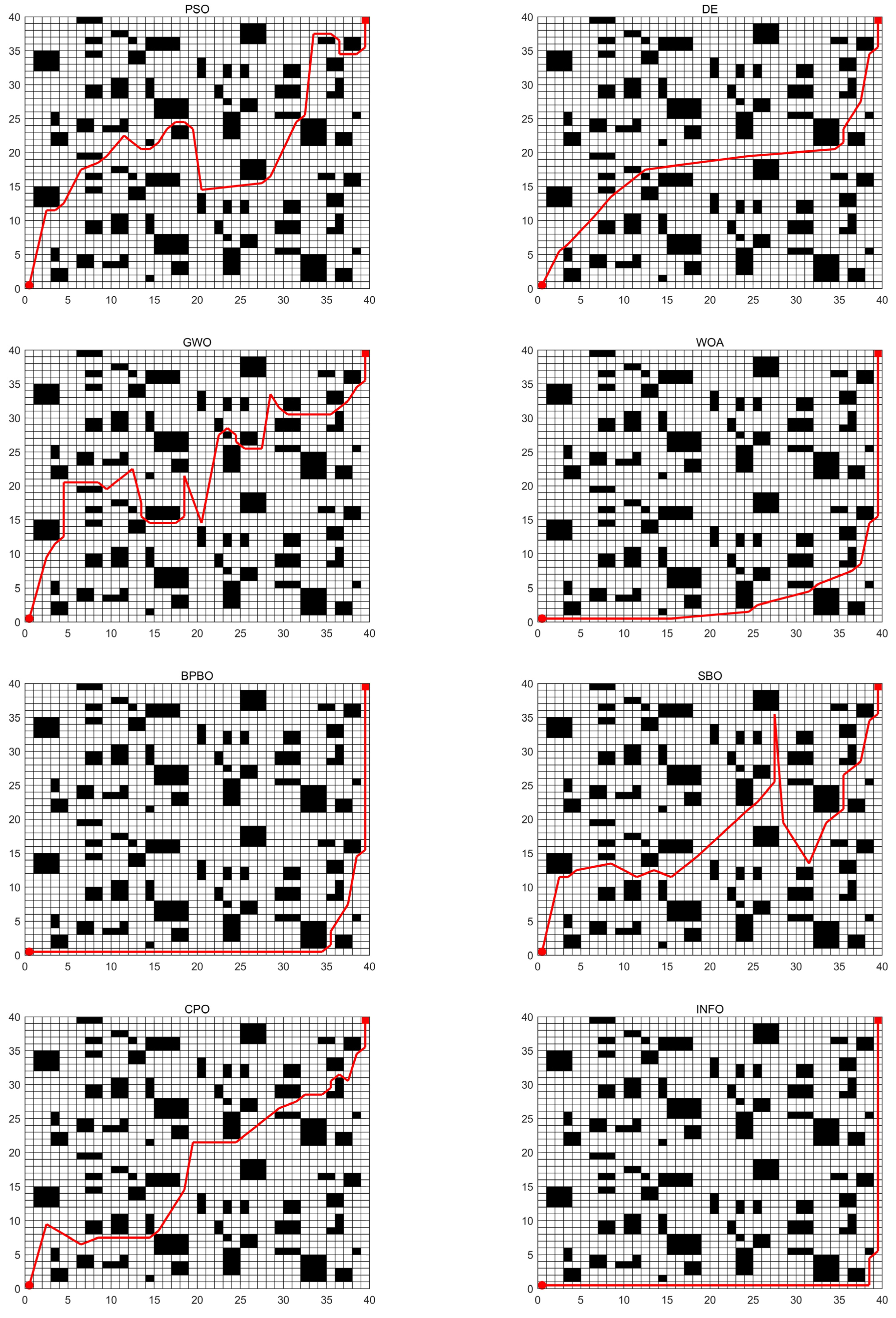
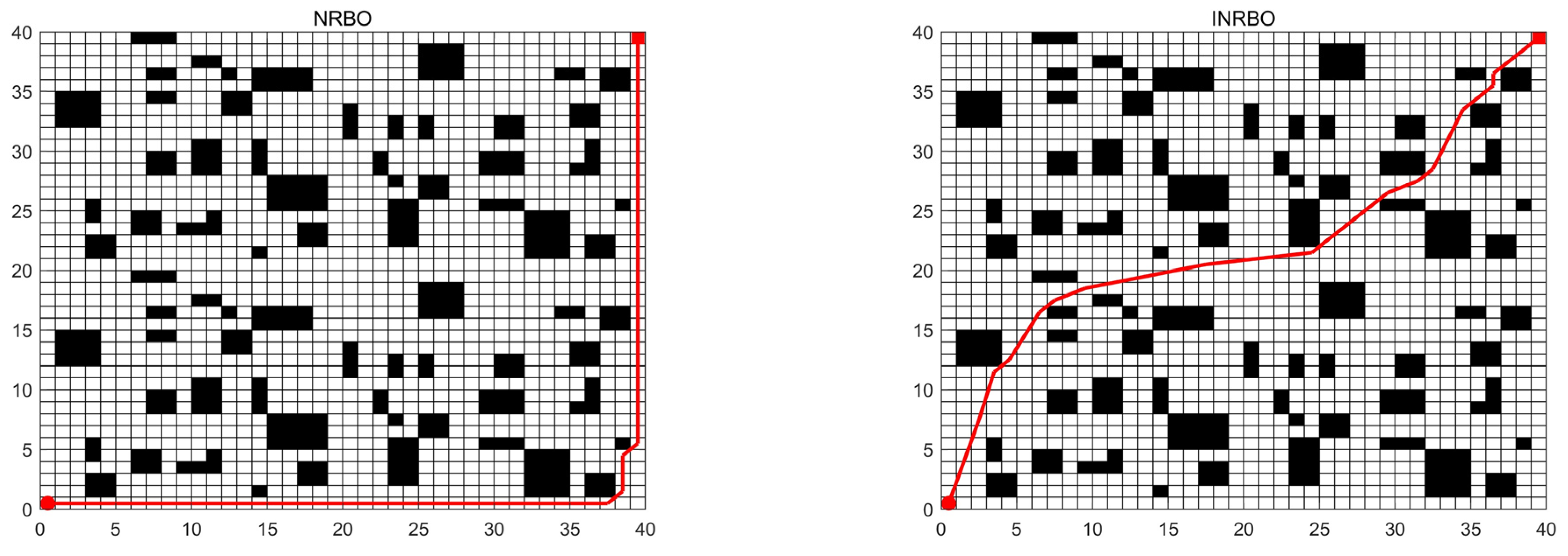
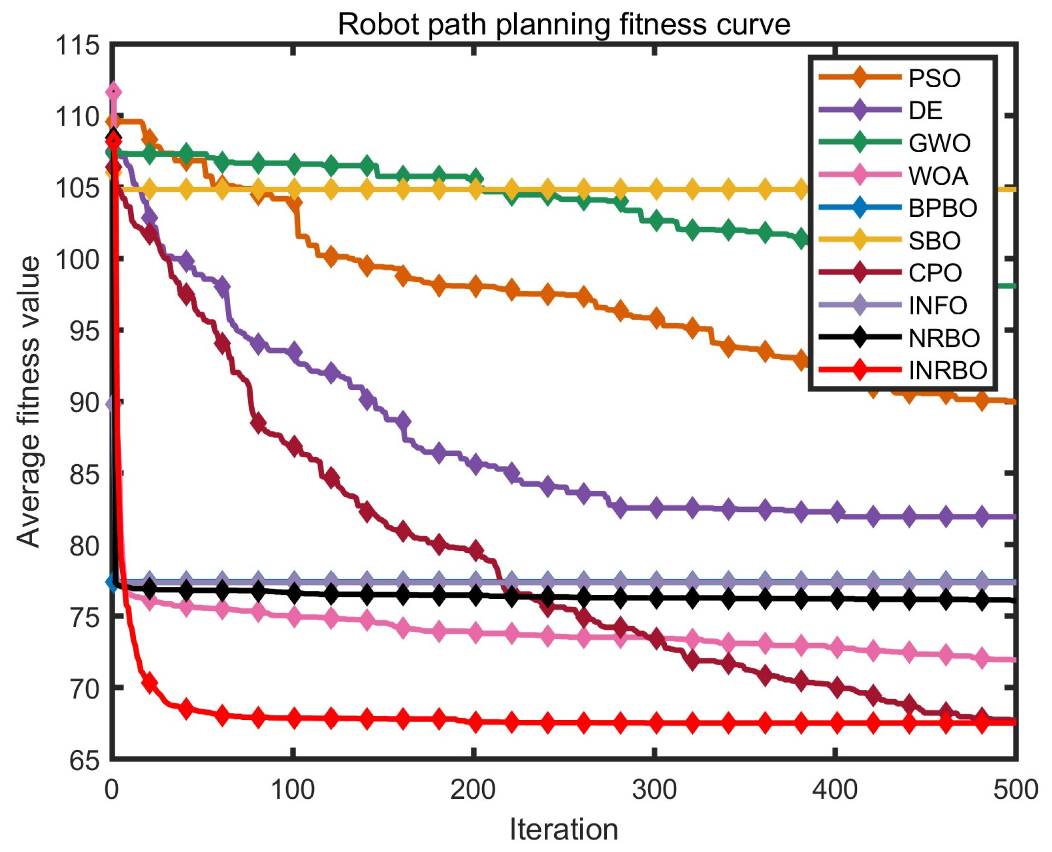
In the 40 × 40 grid environment, the starting point was set at (1,1) and the target at (40,40). Simulations were conducted using INRBO and the nine comparative algorithms. Compared with the smaller 20 × 20 scenario, the 40 × 40 grid features a denser distribution of obstacles and a higher-dimensional search space, placing more stringent demands on the algorithms’ global exploration capability and local optimization accuracy. The simulation results are shown in Figure 13, the changes in fitness values are illustrated in Figure 14, and the comparative data of all ten algorithms are summarized in

Table 9. Quantitative path planning outcomes across algorithms in a 40 × 40 grid setting (Bold formatting indicates the best values).

Algorithm	Ave	Std	Max	Min	Rank
PSO	89.9507	8.6296	109.2625	75.4423	8
DE	81.9475	13.9655	111.7473	64.8829	7
GWO	98.0793	14.4833	123.8104	63.7126	9
WOA	71.9440	2.6548	76.8284	67.9204	3
BPBO	77.4142	0.0000	77.4142	77.4142	6
SBO	104.8228	10.9201	127.4088	77.4142	10
CPO	67.7549	2.2813	72.9301	63.5931	2
INFO	77.3556	0.1787	77.4142	76.8284	5
NRBO	76.0896	1.3042	77.4142	72.9691	4
INRBO	67.5381	2.0277	70.9505	59.4015	1

.

From the perspective of path topology (Figure 13), the paths planned by INRBO exhibit a triple advantage of “global optimality–local smoothness–obstacle avoidance safety.” Compared with the multi-segment detours in PSO paths (e.g., significant obstacle deviations in the grid region (20,25)–(25,30)) and the redundant turns in GWO paths (e.g., ineffective turns in (15,15)–(20,20)), INRBO generates trajectories extending from the start (1,1) to the target (40,40) along an approximately diagonal direction, with no unnecessary detours. Throughout the path, a safe distance of 2–3 grids from obstacles is maintained, fully adapting to the motion constraints of mobile robots. Compared with the local oscillations in the original NRBO paths near (30,30), INRBO trajectories are more regular, with turning angles mostly limited to 45° or 90°, effectively reducing energy consumption and control complexity during robot motion. Although algorithms such as WOA and CPO can generate relatively short paths, they may approach obstacles locally (e.g., CPO path at (25,28) is only one grid from an obstacle) or risk path discontinuities (e.g., WOA path near (18,22) approaches a narrow passage), increasing collision probability in practical applications.

The convergence dynamics further highlight INRBO’s efficiency advantage (Figure 14). Its fitness curve drops rapidly from above 100 to below 70 within the first 150 iterations, approximately 35% faster than the second-ranked CPO. After 300 iterations, the fitness stabilizes around 68, entering the fine-tuning phase with no obvious plateau or oscillation. In contrast, NRBO, INFO, and other algorithms remain above 75, with significant fluctuations (e.g., NRBO fitness varies by 3.5 between 300 and 400 iterations). This behavior arises from INRBO’s adaptive differential operator and elite population genetic strategy: the former uses a dynamically decaying scaling factor (from 0.5 to 0.2) to enable large-step early exploration and quickly locate high-quality global path regions; the latter applies elite pool crossover to inherit high-quality genes, preventing the population from being trapped in local optima. Together, they overcome the traditional algorithm shortcomings of “low exploration efficiency” or “premature convergence” in medium-scale scenarios.

Quantitative metrics (Table 9) further confirm INRBO’s overwhelming performance. Its average path length (67.5381) is 11.24% shorter than the original NRBO (76.0896) and 0.32% shorter than CPO (67.7549), making it the only algorithm with an average path length below 68. The shortest path length (59.4015) surpasses the lower bound of all comparative algorithms, 12.54% shorter than WOA (67.9204) and 6.59% shorter than CPO (63.5931), demonstrating strong optimal solution discovery capability. In terms of stability, INRBO’s standard deviation (2.0277) is only 14.5% of DE (13.9655) and 14.0% of GWO (14.4833). The difference between the maximum path length (70.9505) and the minimum is only 11.549, far lower than PSO (33.8202) and SBO (50.0), reflecting remarkable robustness. In the comprehensive ranking, INRBO occupies the first position by a clear margin. Its characteristics of “fast convergence–short path generation–high stability” in medium-scale complex grid environments fully meet the efficient navigation requirements of mobile robots in scenarios such as industrial workshops and warehouse logistics.

4.2.3. Experimental Analysis in the 60 × 60 Grid Environment

In the 60 × 60 grid environment, the starting point was set at (1,1) and the target at (60,60). Simulations were conducted using INRBO and the nine comparative algorithms. Compared with the 20 × 20 and 40 × 40 scenarios, the 60 × 60 grid features higher obstacle density and a search space expanded to 3600 cells, placing extreme demands on the algorithms’ global exploration breadth, local optimization accuracy, and resistance to dimensional interference. The simulation results are shown in Figure 15, the changes in fitness values are illustrated in Figure 16, and the comparative data of all ten algorithms are summarized in

Table 10. Quantitative path planning outcomes across algorithms in a 60 × 60 grid setting (Bold formatting indicates the best values).

Algorithm	Ave	Std	Max	Min	Rank
PSO	205.9757	18.0360	239.0473	162.4146	6
DE	203.3404	18.6150	232.2655	165.9055	5
GWO	212.0061	13.9498	243.2480	177.6451	10
WOA	118.1208	15.5154	161.3156	91.2790	2
BPBO	206.3294	12.7253	222.5510	176.0004	8
SBO	208.4505	13.9261	232.1470	179.4558	9
CPO	146.6208	9.0579	166.2890	124.8549	3
INFO	206.1386	13.2410	231.1901	176.8493	7
NRBO	203.0418	15.2307	241.7247	175.0327	4
INRBO	108.1501	12.3250	148.7002	91.2144	1

.

From the perspective of path spatial distribution (Figure 15), the paths planned by INRBO exhibit a triple core advantage of “global shortest path–trajectory smoothness–obstacle avoidance safety.” Compared with the large detours in PSO paths (e.g., in the grid region (30,35)–(40,45)) and the redundant obstacle avoidance in GWO paths (e.g., in (25,20)–(35,30)), INRBO generates trajectories extending from the start (1,1) to the target (60,60) along an approximately optimal diagonal direction, with no obvious detours. Throughout the path, a safe buffer of 2–4 grids from obstacles is maintained, fully adhering to the mobile robot’s eight-neighborhood movement rules and safety requirements. Compared with the local oscillations in the original NRBO paths near (45,40), which involve multiple small-angle turns, INRBO paths maintain turning angles mostly at 45° or 90°, with stronger trajectory continuity, effectively reducing energy consumption and control complexity during robot motion. While algorithms such as CPO and WOA can generate relatively short paths, they exhibit critical shortcomings: the CPO path near (35,38) approaches obstacles (only one grid away), and the WOA path in (20,25)–(25,30) passes through a narrow channel, which may increase collision risk due to positioning errors in practical applications. INRBO avoids such safety hazards throughout the entire path, demonstrating superior engineering practicality.

The convergence dynamics further highlight INRBO’s efficiency advantage (Figure 16). Its fitness curve rapidly drops from above 200 to below 120 within the first 200 iterations, achieving approximately 40% faster convergence than the second-ranked WOA. After 300 iterations, the fitness stabilizes around 110, entering the fine-tuning stage with no noticeable plateau or oscillation. This performance stems from the synergy of INRBO’s three core strategies: the adaptive differential operator uses a dynamically decaying scaling factor (from 0.5 linearly down to 0.2) to enable large-step early exploration and quickly cover the large-scale search space; the secondary interpolation strategy leverages global best solutions and high-quality random individuals to directionally search for optimal path directions, avoiding blind exploration; and the elite population genetic strategy applies crossover of high-quality path genes from the elite pool, preventing the population from falling into local optima. Together, these strategies form a closed loop of “broad exploration–directional optimization–elite inheritance,” effectively addressing the core shortcomings of traditional algorithms in large-scale scenarios: low exploration efficiency, premature convergence, and poor solution accuracy.

Quantitative metrics (Table 10) further confirm INRBO’s overwhelming performance. Its average path length (108.1501) is 46.73% shorter than the original NRBO (203.0418) and 8.44% shorter than the second-ranked WOA (118.1208), making it the only algorithm with an average path length below 110. The improvement over CPO (146.6208) and PSO (205.9757) exceeds 26%. The shortest path length (91.2144) surpasses the lower bound of all comparative algorithms, nearly matching WOA’s shortest path (91.2790), and significantly outperforming CPO (124.8549) and DE (165.9055), demonstrating strong optimal solution discovery capability. In terms of stability, INRBO’s standard deviation (12.3250) is only 68.3% of PSO (18.0360) and 66.2% of DE (18.6150). The difference between the maximum path length (148.7002) and the minimum is only 57.4858, far lower than GWO (65.6029) and SBO (52.6912). Especially in large-scale scenarios, where most algorithms suffer dramatic stability degradation due to the expanded search space (e.g., GWO standard deviation reaches 13.9498), INRBO maintains excellent robustness. In the comprehensive ranking, INRBO occupies the first position by a clear margin. Its characteristics of “fast convergence–short path generation–high stability–strong safety” in large-scale complex grid environments fully meet the efficient and safe navigation requirements of mobile robots in urban emergency rescue, large industrial park inspection, and other complex scenarios, laying a solid foundation for the algorithm’s engineering application.

Synthesizing the experimental results from the 20 × 20, 40 × 40, and 60 × 60 grid environments (Figure 11, Figure 12, Figure 13, Figure 14, Figure 15 and Figure 16, Table 8, Table 9 and Table 10), INRBO demonstrates the core characteristics of “strong scalability, stable performance advantage, and outstanding engineering value” in mobile robot path planning tasks. Its overall performance shows an “increasing advantage” trend as grid scale expands, comprehensively surpassing comparative algorithms such as PSO, DE, and NRBO. In the small-scale scenario (20 × 20), INRBO leverages the local fine-search capability of the secondary interpolation strategy to achieve dual optimality in path length and stability, with an average path length reduced by 6.97% compared to the original NRBO and a standard deviation of only 0.3358. In the medium-scale scenario (40 × 40), the dynamic exploration advantage of the adaptive differential operator becomes prominent, improving convergence speed by 35% over CPO, reducing the average path length below the 68-unit threshold, and further enhancing safety distance control accuracy. In the large-scale scenario (60 × 60), the elite population genetic strategy synergizes deeply with the previous two strategies to effectively counter the “curse of dimensionality.” Not only is the average path length reduced by 46.73% compared to NRBO, but INRBO also maintains a low standard deviation of 12.3250 even as most other algorithms experience severe stability degradation, while avoiding practical engineering risks such as paths too close to obstacles or trajectory oscillations.

5. Conclusions and Prospects

This study addresses the core limitations of the traditional Newton–Raphson Based Optimization algorithm (NRBO) in global optimization and practical path-planning tasks, including exploration-exploitation imbalance, insufficient local precision, and loss of high-quality genes, by proposing an improved escape algorithm (INRBO). The algorithm constructs an efficient optimization framework through the synergistic integration of three innovative strategies: the adaptive differential operator dynamically adjusts the scaling factor, enabling large-step exploration in the early iterations and fine-grained optimization in later stages; the secondary interpolation strategy leverages high-quality population information to build interpolation functions, enhancing the directionality and efficiency of local optimum exploitation; and the elite population genetic strategy, through elite pool construction and crossover-mutation operations, ensures stable inheritance of high-quality genes while maintaining moderate innovation. Numerical experiments and application validation indicate that INRBO significantly outperforms nine mainstream algorithms—including PSO, DE, and NRBO—in optimization accuracy and convergence speed across single-peak, multi-peak, hybrid, and composite functions in the CEC2017 test suite. Moreover, in 20 × 20, 40 × 40, and 60 × 60 grid environments for mobile robot path planning, INRBO consistently generates shorter, smoother, and safer paths, demonstrating strong scenario adaptability and practical engineering value.

Despite INRBO’s outstanding performance in static grid environments for numerical optimization and single-robot path planning, several avenues for further development remain. The current study is based on static environment models, whereas real-world scenarios such as firefields involve dynamic changes including heat diffusion, smoke movement, and temporary obstacle formation. Future work will focus on dynamic environment modeling and real-time replanning techniques, integrating real-time sensor data to design adaptive response mechanisms that allow the algorithm to rapidly adjust path strategies in response to sudden environmental changes. Additionally, the present study is limited to single-robot path planning; multi-robot collaboration offers greater efficiency in emergency response, industrial inspection, and other scenarios. Subsequent research will explore INRBO’s application in multi-robot systems, designing inter-robot communication protocols and conflict-avoidance rules to achieve coordinated task allocation and path optimization.

Furthermore, considering the hardware resource constraints of embedded robotic systems, lightweight optimization of INRBO is an important future direction. This will involve simplifying computational procedures, optimizing parameter iteration logic, and reducing redundant operations to lower computational complexity and resource usage while maintaining algorithmic performance, thereby facilitating practical deployment on embedded platforms. Future research will continue to deepen the theoretical foundations and engineering applications of INRBO through dynamic environment adaptation, multi-robot collaboration, and lightweight optimization, further enhancing the algorithm’s robustness and practical utility in complex real-world scenarios, and providing a more efficient solution for mobile robot autonomous navigation.

References

1. Wan, S.; Zhang, X.; Xu, M.; Wang, W.; Jiang, X. Region-adaptive path planning for precision optical polishing with industrial robots. Opt. Express 2018, 26, 23782–23795. [Google Scholar] [CrossRef] [PubMed]
2. Ying, W.; Wang, Z.; Li, H.; Du, S.; Zhao, M. Intelligent Ship Scheduling and Path Planning Method for Maritime Emergency Rescue. Algorithms 2024, 17, 197. [Google Scholar] [CrossRef]
3. Zhang, S.; Xiao, J.; Liu, Y.; Dong, M.; Zhou, Z. A multi-strategy improved sparrow search algorithm for indoor AGV path planning. J. Intell. Fuzzy Syst. 2024, 47, 55–69. [Google Scholar] [CrossRef]
4. Baik, S.; Bong, J.H.; Jeong, S. Weight-Incorporating A* Algorithm with Multi-Factor Cost Function for Enhanced Mobile Robot Path Planning. Actuators 2025, 14, 369. [Google Scholar] [CrossRef]
5. Milin, V.; Stanivuk, T.; Skoko, I.; Bulić, T. Dijkstra and A* Algorithms for Algorithmic Optimization of Maritime Routes and Logistics of Offshore Wind Farms. J. Mar. Sci. Eng. 2025, 13, 1863. [Google Scholar] [CrossRef]
6. Sriramulu, R.; Yadav, A.; Pal, S.B. Fast and efficient indoor navigation: A hybrid pathfinding approach using rapidly-exploring random tree (RRT)-connect and Dijkstra’s algorithm. PeerJ Comput. Sci. 2025, 11, e3028. [Google Scholar] [CrossRef]
7. Dai, X.; Wei, Y. Application of Improved Moth-Flame Optimization Algorithm for Robot Path Planning. IEEE Access 2021, 9, 105914–105925. [Google Scholar] [CrossRef]
8. Kennedy, J.; Eberhart, R. Particle swarm optimization. In Proceedings of the ICNN’95—International Conference on Neural Networks, Perth, Australia, 27 November–1 December 1995; Volume 4, pp. 1942–1948. [Google Scholar]
9. Fu, Y.; Liu, D.; Chen, J.; He, L. Secretary bird optimization algorithm: A new metaheuristic for solving global optimization problems. Artif. Intell. Rev. 2024, 57, 123. [Google Scholar] [CrossRef]
10. Fu, S.; Li, K.; Huang, H.; Ma, C.; Fan, Q.; Zhu, Y. Red-billed blue magpie optimizer: A novel metaheuristic algorithm for 2D/3D UAV path planning and engineering design problems. Artif. Intell. Rev. 2024, 57, 134. [Google Scholar] [CrossRef]
11. Amiri, M.H.; Hashjin, N.M.; Montazeri, M.; Mirjalili, S.; Khodadadi, N. Hippopotamus optimization algorithm: A novel nature-inspired optimization algorithm. Sci. Rep. 2024, 14, 5032. [Google Scholar] [CrossRef]
12. Xu, X. Crocodile Ambush Optimization Algorithm: A new bio-inspired metaheuristic algorithm for solving optimization problems. Array 2025, 28, 100529. [Google Scholar] [CrossRef]
13. Wang, T.-L.; Gu, S.-W.; Liu, R.-J.; Chen, L.-Q.; Wang, Z.; Zeng, Z.-Q. Cuckoo catfish optimizer: A new meta-heuristic optimization algorithm. Artif. Intell. Rev. 2025, 58, 326. [Google Scholar] [CrossRef]
14. Hasan, D.O.; Mohammed, H.M.; Abdul, Z.K. Griffon vultures optimization algorithm for solving optimization problems. Expert Syst. Appl. 2025, 276, 127206. [Google Scholar] [CrossRef]
15. Hassan, M.H.; Kamel, S. Supercell thunderstorm algorithm (STA): A nature-inspired metaheuristic algorithm for engineering optimization. Neural Comput. Appl. 2025, 37, 7207–7260. [Google Scholar] [CrossRef]
16. Zhou, T.; Wei, W. Mobile robot path planning based on an improved ACO algorithm and path optimization. Multimed. Tools Appl. 2025, 84, 10899–10922. [Google Scholar] [CrossRef]
17. Qiuyun, T.; Hongyan, S.; Hengwei, G.; Ping, W. Improved Particle Swarm Optimization Algorithm for AGV Path Planning. IEEE Access 2021, 9, 33522–33531. [Google Scholar] [CrossRef]
18. Zhang, R.; Li, S.; Ding, Y.; Qin, X.; Xia, Q. UAV Path Planning Algorithm Based on Improved Harris Hawks Optimization. Sensors 2022, 22, 5232. [Google Scholar] [CrossRef]
19. Zhu, L.; Zhou, G.; Zhou, Y.; Luo, Q.; Huang, H.; Wei, X. Self-adaptive differential evolution-based coati optimization algorithm for multi-robot path planning. Robotica 2025, 43, 959–996. [Google Scholar] [CrossRef]
20. Dai, Y.; Yu, J.; Zhang, C.; Zhan, B.; Zheng, X. A novel whale optimization algorithm of path planning strategy for mobile robots. Appl. Intell. 2022, 53, 10843–10857. [Google Scholar] [CrossRef]
21. Wang, Z.; Ye, X.; Jiang, G.; Yi, Y. Improved Zebra Optimization Algorithm with Multi Strategy Fusion and Its Application in Robot Path Planning. Biomimetics 2025, 10, 354. [Google Scholar] [CrossRef]
22. Wang, Y.; Tong, K.; Fu, C.; Wang, Y.; Li, Q.; Wang, X.; He, Y.; Xu, L. Hybrid path planning algorithm for robots based on modified golden jackal optimization method and dynamic window method. Expert Syst. Appl. 2025, 18, 127808. [Google Scholar] [CrossRef]
23. Zhang, X.; Duan, Y.; Li, X.; Yang, J.; Li, D.; Zhao, R.; Yang, W. Path planning for greenhouse robots using a hybrid Dung beetle algorithm. Intell. Serv. Robot. 2025, 18, 473–497. [Google Scholar] [CrossRef]
24. Zhang, L.; Zhang, Y.; Li, Y. Mobile Robot Path Planning Based on Improved Localized Particle Swarm Optimization. IEEE Sens. J. 2020, 21, 6962–6972. [Google Scholar] [CrossRef]
25. Zhang, C.; Yang, Y.; Chen, W. Multi-strategy ensemble wind driven optimization algorithm for robot path planning. Math. Comput. Simul. 2024, 231, 144–159. [Google Scholar] [CrossRef]
26. Cui, J.; Wu, L.; Huang, X.; Xu, D.; Liu, C.; Xiao, W. Multi-strategy Adaptable Ant Colony Optimization Algorithm and Its Application in Robot Path Planning. Knowl. Based Syst. 2024, 288, 111459. [Google Scholar] [CrossRef]
27. Sowmya, R.; Premkumar, M.; Jangir, P. Newton-Raphson-based optimizer: A new population-based metaheuristic algorithm for continuous optimization problems. Eng. Appl. Artif. Intell. 2024, 128, 107532. [Google Scholar] [CrossRef]
28. Xu, G.; Yang, F.; Yuan, Y.; Ding, J.; Ji, W.; Zhao, H. Newton–Raphson-based optimizer guided feature mode decomposition and Hilbert transform for pressure pulsation analysis in a tubular pump. Phys. Fluids 2025, 37, 065115. [Google Scholar] [CrossRef]
29. Ru, X.; Qiao, A.; He, K.; Xue, D.; Yang, F. Improved Newton-Raphson-based optimizer with gap evolution strategy for multiple engineering problems. Appl. Math. Model. 2026, 151, 116425. [Google Scholar] [CrossRef]
30. Ghasemi, M.; Akbari, M.A.; Zare, M.; Mirjalili, S.; Deriche, M.; Abualigah, L.; Khodadadi, N. Birds of prey-based optimization (BPBO): A metaheuristic algorithm for optimization. Evol. Intell. 2025, 18, 88. [Google Scholar] [CrossRef]
31. Wu, G.; Mallipeddi, R.; Suganthan, P. Problem Definitions and Evaluation Criteria for the CEC 2017 Competition and Special Session on Constrained Single Objective Real-Parameter Optimization; Nanyang Technological University: Singapore, 2016. [Google Scholar]
32. Storn, R.; Price, K. Differential evolution–a simple and efficient heuristic for global optimization over continuous spaces. J. Glob. Optim. 1997, 11, 341–359. [Google Scholar] [CrossRef]
33. Mirjalili, S.; Mirjalili, S.M.; Lewis, A. Grey Wolf Optimizer. Adv. Eng. Softw. 2014, 69, 46–61. [Google Scholar] [CrossRef]
34. Mirjalili, S.; Lewis, A. The Whale Optimization Algorithm. Adv. Eng. Softw. 2016, 95, 51–67. [Google Scholar] [CrossRef]
35. Wang, J.; Chen, Y.; Lu, C.; Heidari, A.A.; Wu, Z.; Chen, H. The status-based optimization: Algorithm and comprehensive performance analysis. Neurocomputing 2025, 647, 130603. [Google Scholar] [CrossRef]
36. Abdel-Basset, M.; Mohamed, R.; Abouhawwash, M. Crested Porcupine Optimizer: A new nature-inspired metaheuristic. Knowl. Based Syst. 2024, 284, 111257. [Google Scholar] [CrossRef]
37. Ahmadianfar, I.; Heidari, A.A.; Noshadian, S.; Chen, H.; Gandomi, A.H. INFO: An efficient optimization algorithm based on weighted mean of vectors. Expert Syst. Appl. 2022, 195, 116516. [Google Scholar] [CrossRef]
38. Chen, Z.; Fu, B.; Yang, Y. A Novel Elite-Guided Hybrid Metaheuristic Algorithm for Efficient Feature Selection. Biomimetics 2025, 10, 747. [Google Scholar] [CrossRef]
39. Cao, L.; Wei, Q. SZOA: An Improved Synergistic Zebra Optimization Algorithm for Microgrid Scheduling and Management. Biomimetics 2025, 10, 664. [Google Scholar] [CrossRef]
40. Chen, Y.; Sun, R.; Zheng, J.; Shao, Y.; Zhou, H. MEIAO: A Multi-Strategy Enhanced Information Acquisition Optimizer for Global Optimization and UAV Path Planning. Biomimetics 2025, 10, 765. [Google Scholar] [CrossRef]
41. Wang, Z.; Tang, J.; Yi, F.; Ren, X.; Wang, K. Research on path planning of robotic arms based on DAPF-RRT algorithm. PLoS ONE 2025, 20, e0323734. [Google Scholar] [CrossRef]
42. Gao, Y.; Jiang, Q.; Wang, M.; Dong, X. Advances in Path-Planning Algorithms for Agricultural Robots. J. Field Robot. 2025, 43, 89–145. [Google Scholar] [CrossRef]
43. Fang, Y.; He, J.; Wang, X.; Xu, W.; Kim, J.I.; Chen, X. A* Algorithm for On-Site Collaborative Path Planning in Building Construction Robots. Buildings 2025, 15, 3876. [Google Scholar] [CrossRef]
Figure 1. Performance curves of NRBO under different enhancement strategies.
Symmetry 18 00280 g001aSymmetry 18 00280 g001b
Figure 2. Average rankings of enhanced NRBO variants.
Symmetry 18 00280 g002
Figure 3. Comparison of convergence speed of different algorithms on CEC2017 test set.
Symmetry 18 00280 g003aSymmetry 18 00280 g003bSymmetry 18 00280 g003c
Figure 4. Boxplot analysis for different algorithms on CEC2017 the test set.
Symmetry 18 00280 g004aSymmetry 18 00280 g004bSymmetry 18 00280 g004c
Figure 5. Comparison of convergence speed of different algorithms on CEC2022 test set.
Symmetry 18 00280 g005
Figure 6. Boxplot analysis for different algorithms on the test set.
Symmetry 18 00280 g006
Figure 7. The analysis of the population diversity of INRBO and NRBO.
Symmetry 18 00280 g007
Figure 8. Comparison of convergence speed of different algorithms on CEC2017 test set.
Symmetry 18 00280 g008aSymmetry 18 00280 g008bSymmetry 18 00280 g008c
Figure 9. Distributions of the relative performance rankings achieved by each tested algorithm.
Symmetry 18 00280 g009
Figure 10. Architectural model of the two-dimensional cell space.
Symmetry 18 00280 g010
Figure 11. Paths generated by various planners in a 20 × 20 grid environment.
Symmetry 18 00280 g011aSymmetry 18 00280 g011b
Figure 12. Fitness evolution for each tested method across iterations on a 20 × 20 cell map.
Symmetry 18 00280 g012
Figure 13. Paths generated by various planners in a 40 × 40 grid environment.
Symmetry 18 00280 g013aSymmetry 18 00280 g013b
Figure 14. Fitness evolution for each tested method across iterations on a 40 × 40 cell map.
Symmetry 18 00280 g014
Figure 15. Paths generated by various planners in a 60 × 60 grid environment.
Symmetry 18 00280 g015aSymmetry 18 00280 g015b
Figure 16. Fitness evolution for each tested method across iterations on a 60 × 60 cell map.
Symmetry 18 00280 g016