Article

Bayesian-Optimized Explainable AI for CKD Risk Stratification: A Dual-Validated Framework

1
School of Computer Application, Guilin University of Technology, Guilin 541004, China
2
School of Electronic Information and Artificial Intelligence, Wuzhou University, Wuzhou 543000, China
*
Author to whom correspondence should be addressed.
Symmetry 2026, 18(1), 81; https://doi.org/10.3390/sym18010081
Submission received: 7 December 2025 / Revised: 22 December 2025 / Accepted: 31 December 2025 / Published: 3 January 2026

Abstract

Chronic kidney disease (CKD) impacts more than 850 million people globally, yet existing machine learning methodologies for risk stratification encounter substantial challenges: computationally intensive hyperparameter tuning, model opacity that conflicts with clinical interpretability standards, and class imbalance leading to systematic prediction bias. We constructed an integrated architecture that combines XGBoost with Optuna-driven Bayesian optimization, evaluated against 19 competing hyperparameter tuning approaches and tested on CKD patients using dual-paradigm statistical validation. The architecture delivered 93.43% accuracy, 93.13% F1-score, and 97.59% ROC-AUC—representing gains of 6.22 percentage points beyond conventional XGBoost and 7.0–26.8 percentage points compared to 20 baseline algorithms. Tree-structured Parzen Estimator optimization necessitated merely 50 trials compared to 540 for grid search and 1069 for FLAML, whereas Boruta feature selection accomplished 54.2% dimensionality reduction with no performance compromise. Over 30 independent replications, the model exhibited remarkable stability (cross-validation standard deviation: 0.0121, generalization gap: −1.13%) alongside convergent evidence between frequentist and Bayesian paradigms (all p < 0.001, mean CI-credible interval divergence < 0.001, effect sizes d = 0.665–5.433). Four separate explainability techniques (SHAP, LIME, accumulated local effects, Eli5) consistently identified CKD stage and albumin-creatinine ratio as principal predictors, aligning with KDIGO clinical guidelines. Clinical utility evaluation demonstrated 98.4% positive case detection at 50% screening threshold alongside near-optimal calibration (mean absolute error: 0.138), while structural equation modeling revealed hyperuricemia (β = −3.19, p < 0.01) as the most potent modifiable risk factor. This dual-validated architecture demonstrates that streamlined hyperparameter optimization combined with convergent multi-method interpretability enables precise CKD risk stratification with clinical guideline alignment, supporting evidence-informed screening protocols.

1. Introduction

Progressive renal dysfunction affects more than 850 million individuals worldwide, contributing to roughly 2.4 million annual deaths and imposing considerable healthcare expenditure burdens [1,2]. The asymptomatic character of early-stage kidney deterioration leads to delayed diagnosis when therapeutic interventions become substantially constrained [3]. Precise risk stratification during pre-dialysis phases facilitates targeted intervention strategies that may decelerate functional decline toward end-stage disease, yet conventional assessment frameworks relying on isolated biomarker thresholds exhibit inadequate sensitivity for capturing multifactorial disease pathophysiology [4,5].
Machine learning applications in nephrology have progressed considerably over the past decade. Initial implementations using decision trees and support vector machines attained modest discrimination on limited cohorts, while contemporary ensemble architectures including random forests and gradient boosting frameworks report accuracies spanning from 85% to 95% [6,7,8]. Recent benchmarking investigations reveal that XGBoost, LightGBM, and CatBoost consistently surpass traditional statistical models for structured clinical data [9,10]. Despite these technical advances, clinical adoption remains constrained by three core barriers: computationally demanding hyperparameter optimization necessitating thousands of training iterations, algorithmic opacity conflicting with clinical transparency standards, and class imbalance inducing systematic bias toward majority classifications at the cost of high-risk patient detection [11].
Bayesian optimization frameworks provide potential solutions through intelligent parameter space exploration. Tree-structured Parzen Estimator algorithms have exhibited order-of-magnitude reductions in function evaluations while preserving superior performance across diverse applications [12]. Concurrently, model-agnostic interpretation methods—including SHAP, LIME, and accumulated local effects—deliver mathematically rigorous frameworks for quantifying feature contributions [13]. Wrapper-based feature selection algorithms such as Boruta facilitate systematic identification of informative variables while eliminating redundant features [14]. However, no systematic comparison has assessed contemporary optimization algorithms specifically for CKD prediction, nor has multi-method interpretability convergence been examined. Furthermore, statistical validation predominantly depends on frequentist frameworks (p-values, confidence intervals) that struggle to quantify evidence strength gradients and are frequently misinterpreted, while Bayesian approaches furnishing direct probability statements about model superiority remain underutilized despite advocated advantages in recent medical research [15]. Quantification of clinical utility through decision-analytic frameworks also remains underexplored despite being essential for deployment recommendations.
We constructed an integrated framework combining XGBoost with Optuna-driven Bayesian optimization, benchmarked against 19 alternative hyperparameter strategies. Boruta feature selection enables 54.2% dimensionality reduction without performance degradation, while comprehensive explainability analysis integrating SHAP, LIME, Eli5, and ALE provides convergent evidence regarding feature relevance. Dual-paradigm statistical validation synthesizes Bayesian (posterior distributions, Bayes factors, credible intervals) and frequentist inference (p-values, confidence intervals, effect sizes) across 30 independent replications with mean CI-credible interval divergence <0.001, while macro-averaged metrics and stratified cross-validation address class imbalance.
Our principal contributions include
(1) Optuna-driven Bayesian optimization necessitating merely 50 trials versus 540 for grid search and 1069 for FLAML while attaining F1: 93.13% and ROC-AUC: 97.59%;
(2) Multi-method explainability convergence across SHAP, LIME, Eli5, and ALE consistently identifying CKD stage and albumin-creatinine ratio as co-primary determinants concordant with KDIGO guidelines;
(3) Bayesian-Frequentist dual validation framework attaining convergent evidence across paradigms (all p < 0.001, CI-credible interval divergence <0.001) through 30 independent iterations;
(4) Comprehensive performance superiority over 20 baseline algorithms with exceptional stability (CV standard deviation: 0.0121, generalization gap: −1.13%), exceeding standard XGBoost by 6.22 percentage points;
(5) Clinical utility quantification with 98.4% positive case capture at 50% screening and near-optimal calibration (mean absolute error: 0.138);
(6) Structural equation modeling revealing hyperuricemia (β = −3.19, p < 0.01) as the most potent modifiable risk factor.

2. Related Works

Initial machine learning applications to CKD classification predominantly utilized the publicly available UCI CKD dataset (n = 400), where Rahman et al. [16] attained 99.75% accuracy using ensemble methods with MICE imputation and Borderline-SMOTE, while Yang et al. [17] documented negligible performance differences across eleven algorithms, most surpassing 98% accuracy. Metherall et al. [18] and Khan et al. [19] similarly accomplished >98% and 91.7% accuracy, respectively, using random forests and SVM. Such near-optimal performance on simplified benchmarks raises concerns: when diverse algorithms attain virtually identical results (>98%), this convergence reflects task simplicity rather than algorithmic advancement. More critically, most existing studies implement binary classification (presence/absence), neglecting the multi-class risk stratification essential for clinical decision-making where nuanced severity assessment guides intervention strategies. Reddy et al. [20] demonstrated this limitation—while attaining high internal performance (ROC-AUC 0.94–0.98), their model exhibited degradation upon exposure to authentic clinical distributions, underscoring the gap between controlled benchmarks and real-world heterogeneity.
Contemporary hyperparameter optimization exhibits efficiency constraints [21]. Grid search experiences exponential scaling with dimensionality [22], rendering exhaustive exploration computationally prohibitive for modern ensemble architectures. Random search provides no convergence guarantees—reported accuracies of 100% [23] and 99.16% [24] on small datasets often reflect overfitting artifacts rather than optimization efficacy, particularly when nested cross-validation is absent. Evolutionary strategies demonstrate inconsistent behavior: Luaha et al. [25] documented dramatic 18.75-percentage-point improvements using genetic algorithms over grid search (98.75% vs. 80%), yet such gaps typically signal misconfigured baselines or validation contamination rather than genuine algorithmic superiority. Bayesian optimization frameworks, despite theoretical advantages, encounter implementation pitfalls including unfair baseline comparisons [26]—optimized methods versus unoptimized competitors—that artificially inflate performance gains, while Liu et al. [27] demonstrated information leakage through using validation accuracy as optimization objectives within non-nested schemes. These inefficiencies motivate principled Bayesian approaches that balance exploration-exploitation trade-offs through statistically grounded acquisition functions.
Post hoc interpretation methods address model opacity through feature attribution, with SHAP (SHapley Additive exPlanations) becoming prevalent across CKD prediction [28,29,30,31,32] and acute kidney injury forecasting [33]. However, critical limitations persist. Studies predominantly implement SHAP in isolation [30,32,33] without cross-validating against complementary techniques (LIME, ALE, permutation importance), leaving explanation robustness unverified. When multiple methods are applied [31], conflicting feature importance hierarchies emerge—LIME versus SHAP rankings diverge substantially—yet no principled framework exists for adjudicating which explanation merits clinical trust. This single-method dependency creates interpretability fragility: conclusions derived from one attribution technique may contradict insights from alternative approaches, undermining clinician confidence. Furthermore, SHAP attributions often remain unvalidated by domain experts [32,33], and statistical feature importance frequently conflicts with clinical reasoning. Jawad et al. [31] discovered highly ranked features (specific gravity, pus cell count) lack diagnostic significance per nephrologist consultation, while essential biomarkers (eGFR, HbA1C) were absent from datasets. This exposes confusion between predictive correlation and causal mechanisms—interpretation methods uniformly present associations as actionable targets, yet features exhibiting strong statistical importance may be disease consequences rather than modifiable causes.
Sequential feature selection pipelines combining multiple algorithms have proliferated without principled justification. Studies implement Boruta-LASSO cascades [34,35] or Boruta-XGBoost combinations [36] as black-box workflows, providing no interpretable rationale for method sequencing. Chen et al. [34] and Qin et al. [35] furnish no theoretical basis for why Boruta’s random forest importance should precede LASSO’s L1 penalty, while Xu et al. [36] fail to justify XGBoost over embedded selection approaches. Feature stability remains critically underexamined—studies report final selected features without assessing consistency across bootstrap samples [34,35,36,37], leaving uncertain whether identified predictors represent robust signals or train-test split artifacts.
Validation methodologies further reveal gaps. Frequentist approaches (p-values, confidence intervals) dominate medical AI evaluation [38,39], yet these methods struggle to quantify evidence strength gradients and are frequently misinterpreted—p-values answer “probability of data under null hypothesis” rather than clinically relevant model superiority probabilities. Goligher et al. [40] illustrated that Bayesian posterior distributions provide direct probability statements about model superiority—expressing results as “95% probability that Model A outperforms B”—offering clinical interpretability beyond binary significance testing. Bayes factors quantify evidence strength continuously rather than through arbitrary thresholds [41,42], yet machine learning validation studies rarely integrate dual-paradigm approaches to leverage complementary inferential strengths [43].

3. Preliminary

3.1. Data Overview

Table 1 presents clinical variables utilized in this investigation. Our analytical cohort comprises 1150 chronic kidney disease patients drawn from a multi-institutional retrospective database, with all personally identifiable information systematically removed to ensure participant confidentiality [44].
The clinical dataset incorporates patient demographics, heritable disease susceptibility, and quantitative laboratory measurements. Genetic predisposition markers document the inherited component of renal pathology, which follows autosomal dominant transmission in roughly 15% of affected individuals, predominantly within polycystic kidney disease and familial nephritis syndromes [45].
Cardiovascular and metabolic comorbidities serve as critical prognostic determinants. Hypertensive vascular disease accelerates nephrosclerotic changes, while diabetes-associated kidney disease constitutes the leading cause of progressive renal impairment. Elevated serum uric acid concentrations induce renal toxicity via crystalline deposits triggering tubular inflammatory responses [46].
Laboratory parameters capture pathophysiological mechanisms driving CKD advancement. The urinary albumin-to-creatinine ratio quantifies glomerular barrier dysfunction, with persistent low-grade albuminuria (30–300 mg/g) marking early nephropathy and substantial proteinuria (exceeding 300 mg/g) indicating established filtration damage. Serum creatinine concentrations provide indirect estimates of functional nephron population, while the estimated glomerular filtration rate, derived through the CKD-EPI formula, delivers standardized renal function assessment [47].
Disease classification adheres to validated KDIGO staging protocols, distinguishing five progressive categories. Initial-stage disease (stages 1–2) retains largely intact filtration performance but demonstrates structural pathology. Intermediate-stage disease (stage 3) marks the crucial transition where compensatory mechanisms fail, triggering mineral dysregulation and metabolic disturbances. Late-stage disease (stages 4–5) encompasses profound functional compromise with uremic metabolite accumulation, mandating preparation for renal replacement therapy [48].
The quaternary risk classification schema integrates diverse clinical indicators to forecast disease trajectory independent of conventional staging. This framework acknowledges that patients occupying equivalent CKD stages may exhibit substantially different clinical outcomes contingent upon proteinuria magnitude and comorbid condition burden, facilitating individualized treatment protocols and rational healthcare resource allocation.

3.2. Exploratory Data Analysis

Figure 1 displays correlational analysis of clinical parameters and renal biomarkers using Pearson coefficients. The matrix visualization encodes correlation strength through sector angles (upper triangle) and numerical values (lower triangle). eGFR demonstrates strong inverse correlations with serum creatinine (r = −0.69), CKD stage (r = −0.91), and progression rate (r = −0.72). These relationships highlight the inverse association between filtration function and disease severity. Among urinary biomarkers, urinary anatomical structure abnormalities (UAS) correlate moderately with urine protein index (r = 0.31) and hyperuricemia (r = 0.36), consistent with shared pathophysiological pathways. Comorbidities such as hypertension and diabetes show expected links with progression markers, while the albumin-to-creatinine ratio (ACR) moderately associates with progression rate (r = 0.49), supporting its clinical relevance. In contrast, demographic variables like gender and genetic background exhibit negligible correlations (|r| < 0.1) with most biomarkers, indicating their limited impact on disease progression in this cohort.
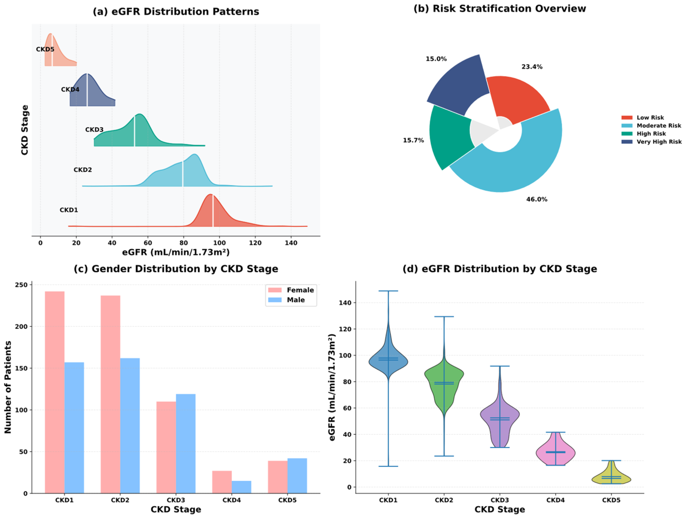
Figure 2 illustrates demographic profiles and functional decline patterns through multiple analytical perspectives. (a) eGFR Distribution Patterns employs kernel density estimation to visualize stage-specific renal function, where early-stage disease (CKD1, coral curve) maintains tight clustering around 100 mL/min/1.73 m2 with minimal spread, while progressive stages demonstrate leftward shifts and broadening distributions, with CKD5 (salmon) exhibiting severely compressed filtration rates near dialysis threshold. Median indicators (white lines) confirm systematic functional deterioration across disease trajectory. (b) Risk Stratification Overview reveals cohort composition through proportional segmentation: moderate risk dominates at 46.0% (529 patients), followed by low risk (23.4%, 269 patients), high risk (15.7%, 180 patients), and very high risk (15.0%, 172 patients), reflecting the preponderance of intermediate disease states in tertiary care settings. (c) Gender Distribution by CKD Stage demonstrates female predominance across stages 1–3 (female-to-male ratio approximately 1.4–1.5:1), with this disparity attenuating in advanced disease stages (stages 4–5 showing more balanced distribution around 1:1), suggesting stage-dependent gender influences may attenuate in end-stage pathology. (d) eGFR Distribution by CKD Stage presents violin plots confirming progressive functional constriction, with interquartile ranges narrowing from 85–115 mL/min/1.73 m2 (CKD1) to 5–15 mL/min/1.73 m2 (CKD5), while median values (horizontal bars) demonstrate stepwise decline consistent with KDIGO staging thresholds.
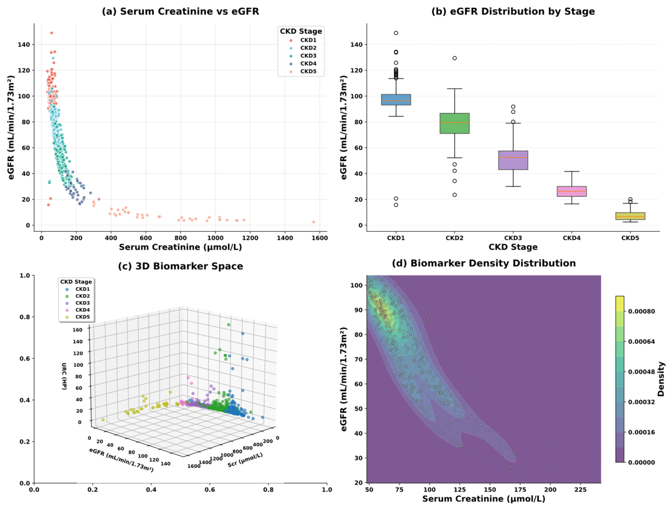
Figure 3 demonstrates interconnected biomarker dynamics through complementary visualization strategies. Panel (a) reveals the characteristic hyperbolic inverse relationship between serum creatinine and eGFR. Early-stage patients (CKD1–2) cluster in the physiological zone (Scr < 150 μmol/L, eGFR > 60 mL/min/1.73 m2). In contrast, advanced stages (CKD4–5) occupy the pathological extremum (Scr > 400 μmol/L, eGFR < 30 mL/min/1.73 m2). This pattern reflects progressive nephron loss and compensatory solute accumulation. Panel (b) quantifies functional decline through box-and-whisker plots. Median eGFR decreases approximately 25 mL/min/1.73 m2 per stage progression. Panel (c) 3D Biomarker Space integrates serum creatinine, eGFR, and urinary RBC count into a three-dimensional decision volume, where stage-specific clustering emerges along the principal axis of renal dysfunction, with mild disease occupying the high-eGFR/low-Scr octant and severe disease migrating toward the opposite vertex, demonstrating clear spatial separation despite moderate overlap in transitional zones. Panel (d) Biomarker Density Distribution employs kernel density estimation with contour mapping to identify regions of high patient concentration, revealing a primary density band along the inverse exponential trajectory (purple core) with elevated density at physiological ranges (50–100 μmol/L Scr, 70–100 mL/min/1.73 m2 eGFR) and secondary accumulation in advanced dysfunction zones, confirming the nonlinear relationship between creatinine generation and glomerular filtration capacity.
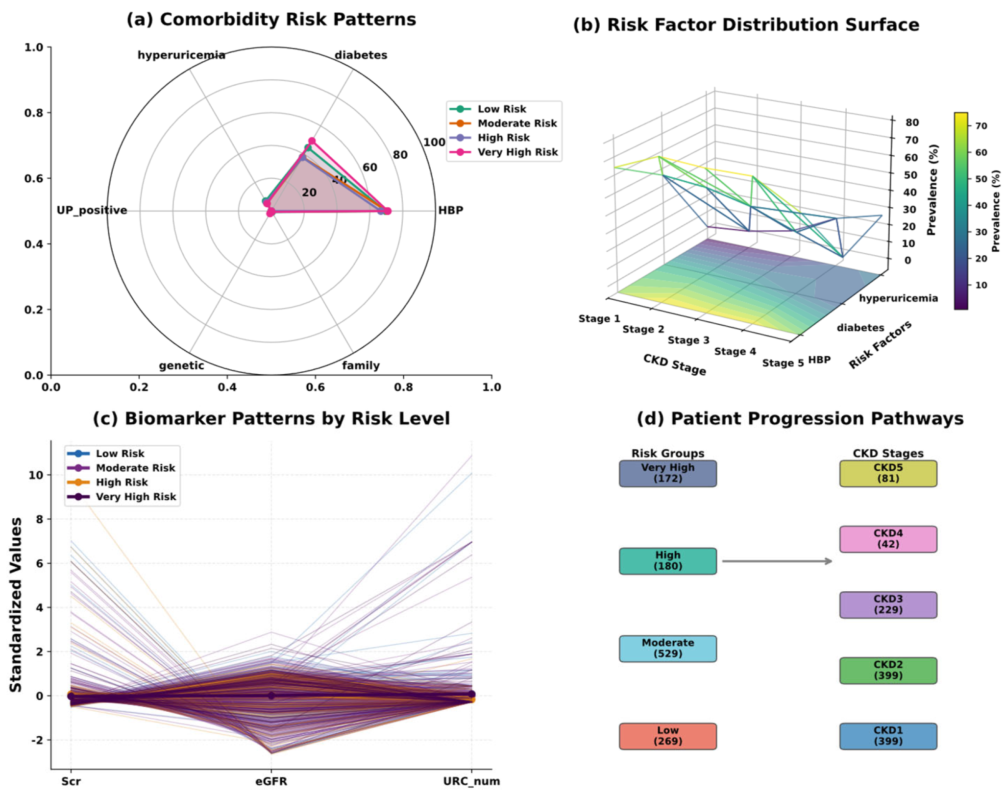
Figure 4 synthesizes comorbidity profiles and risk trajectories across multiple analytical dimensions. (a) Comorbidity Risk Patterns displays polar coordinate representation of six clinical risk factors, revealing convergent profiles across risk strata with diabetes and hypertension exhibiting highest prevalence (50–75% range), while genetic predisposition and family history demonstrate lower penetrance (20–50%), with very high-risk patients (pink trajectory) showing elevated burden across all dimensions compared to low-risk counterparts (teal trajectory). (b) Risk Factor Distribution Surface employs triangular mesh visualization to map comorbidity prevalence across CKD stages, where the topographic landscape transitions from elevated plateaus in early disease (Stage 1–2, prevalence 40–60%) to depressed valleys in advanced stages (Stage 4–5, prevalence 20–40%), with color gradients from yellow (70% prevalence) through turquoise (40%) to purple (10%) illustrating stage-dependent risk factor clustering. (c) Biomarker Patterns by Risk Level utilizes parallel coordinates with standardized z-scores, demonstrating divergent trajectories where very high-risk patients (dark purple lines) exhibit characteristic elevation in serum creatinine (+2 SD) and urinary RBC counts (+1 SD) with corresponding eGFR depression (−2 SD), while low-risk individuals (blue lines) maintain near-zero standardized values across all biomarkers, with mean trajectories (bold lines) confirming systematic separation between risk categories. (d) Patient Progression Pathways illustrates cohort distribution through bidirectional flow representation, where left column enumerates risk groups (Low 269, Moderate 529, High 180, Very High 172 patients) connecting through gray arrows to right column CKD stages (CKD1-5 ranging from 399 to 81 patients), demonstrating the transition from risk-based stratification to physiological staging criteria.
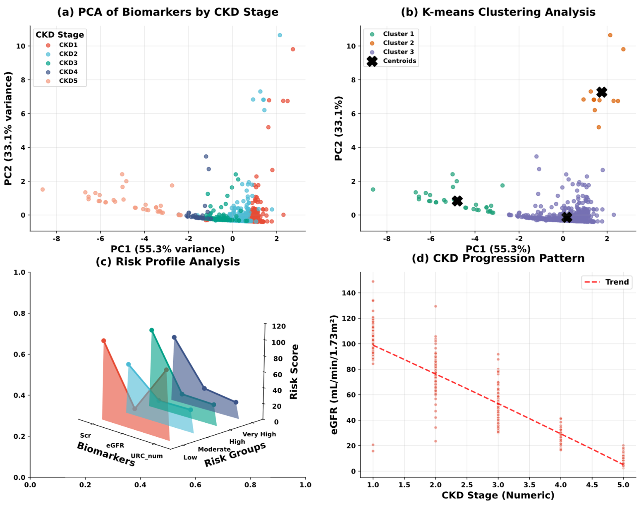
Figure 5 presents advanced analytical approaches for pattern recognition and trajectory prediction. (a) PCA of Biomarkers by CKD Stage achieves 88.4% cumulative variance explanation through two-component decomposition (PC1: 55.3%, PC2: 33.1%), revealing stage-dependent clustering where early disease (CKD1-2, coral/turquoise) occupies negative PC1 space (−8 to 0) with minimal PC2 variation, while advanced stages (CKD4-5, purple/salmon) migrate toward positive PC1 values (0 to +2) with increased PC2 dispersion (0 to +10), indicating progressive biomarker divergence accompanies disease evolution. (b) K-means Clustering Analysis identifies three natural patient subgroups through unsupervised learning, where Cluster 1 (teal, n ≈ 150) concentrates at PC1 = −5/PC2 = 1, Cluster 2 (orange, n ≈ 80) disperses across PC1 = 0–2/PC2 = 6–10, and Cluster 3 (purple, n ≈ 750) dominates the origin vicinity, with black centroid markers (X symbols) defining optimal cluster centers that transcend traditional clinical staging boundaries. (c) Risk Profile Analysis employs 3D waterfall visualization along biomarker–risk group axes, where low-risk patients (coral ribbon) maintain elevated profiles across Scr/eGFR/URC_num dimensions, while very high-risk cases (navy ribbon) demonstrate compressed profiles particularly in eGFR domain, with intermediate risk categories (turquoise/purple ribbons) showing transitional morphologies, and vertical projections indicating risk score magnitudes (0–120 scale). (d) CKD Progression Pattern documents the inverse exponential relationship between stage advancement and renal function through scatter distribution (coral points) overlaid with second-order polynomial regression (red dashed curve, R2 > 0.8), demonstrating accelerating eGFR decline from Stage 1 (median 95 mL/min/1.73 m2) through Stage 5 (median 8 mL/min/1.73 m2), with widening confidence intervals in advanced disease reflecting increased inter-patient variability at low filtration rates.
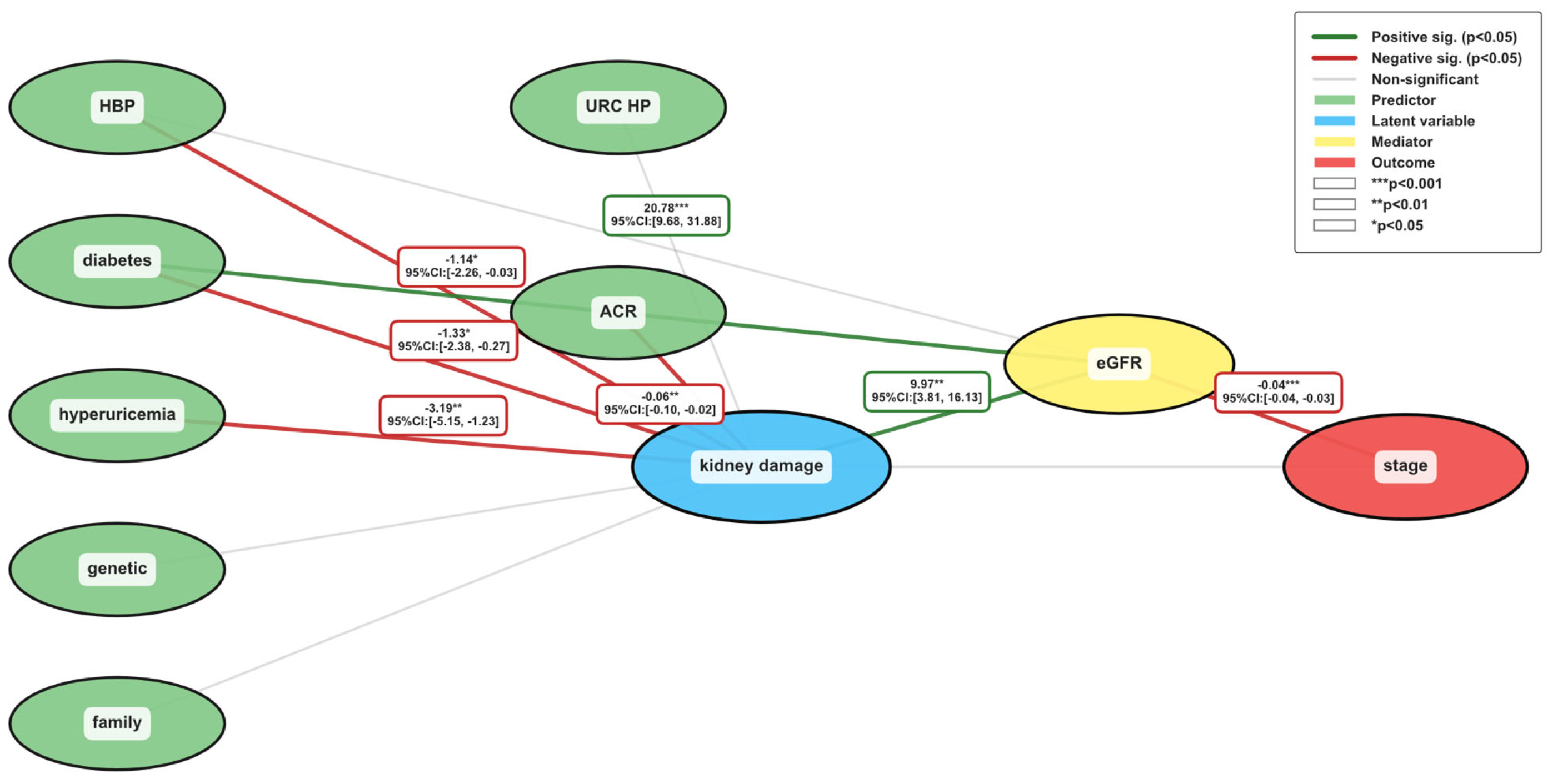
Figure 6 presents the structural equation model (SEM) illustrating causal pathways in CKD progression through latent variable mediation. The model was constructed using semopy (Python 3.11) with maximum likelihood estimation (n = 988). Model fit indices demonstrated excellent fit (CFI = 0.999, TLI = 0.999, RMSEA = 0.008, SRMR = 0.050). The measurement model defines kidney damage as a latent construct (blue ellipse) manifested through two indicators: URC_HP and ACR. The path from kidney damage to ACR shows a factor loading of 20.78 ***, while ACR demonstrates a reciprocal association with kidney damage (β = −0.06 **). Structural pathways reveal hyperuricemia as the strongest direct predictor of kidney damage (β = −3.19 **), followed by diabetes (β = −1.33 *) and hypertension (HBP, β = −1.14 *). Genetic predisposition and family history showed non-significant associations (indicated by gray arrows), suggesting metabolic factors dominate in this cohort. The kidney damage construct influences estimated glomerular filtration rate (eGFR, yellow ellipse; β = 9.97 **), which serves as the primary determinant of CKD stage (red ellipse; β = −0.04 ***). Path coefficients are annotated with significance levels (*** p < 0.001, ** p < 0.01, * p < 0.05). Node colors distinguish variable types: green ellipses represent predictors and observed indicators, blue indicates the latent kidney damage variable, yellow denotes eGFR as a mediator, and red marks the outcome (stage). Green arrows indicate positive associations, while red arrows denote negative relationships; gray arrows represent non-significant paths.
This exploratory investigation laid a robust foundation through the identification of critical predictive associations, validation of data integrity, and demonstration of the dataset’s clinical reliability and consistency over time across collaborating centers.

3.3. Data Processing

The initial cohort comprising 1150 patients with 19 clinical variables underwent comprehensive quality enhancement to ensure analytical robustness. Initial evaluation revealed heterogeneous data characteristics including format inconsistencies among categorical variables, disparate measurement units, and sporadic missing values requiring systematic resolution.
Standardization protocols addressed format heterogeneity across categorical features. Hyperuricemia indicators received binary encoding, while urinary anatomical structure (UAS) assessments underwent unified classification schema implementation. Measurement unit discrepancies in urine red blood cell (URC) counts necessitated conversion to a common HP (high-power field)-based scale:
U R C H P = U R C n u m 10 ,     i f   U R C u n i t = μ l   U R C n u m ,           i f   U R C u n i t = H P  
Modal replacement addressed categorical data gaps, whereas numerical deficits received K-nearest neighbor imputation (k = 5):
x i j ^ = 1 k l N k i x i j
d i , l = m = 1 p x i m x l m 2
Binary variables adopted dichotomous encoding (1/0). Ordinal features preserved inherent ordering: urine protein index (UP_index) maintained 6-tier stratification, while albumin-creatinine ratio (ACR) retained categorical boundaries. Outcome variables encompassed risk grades (0–3) and staging classifications (0–4).
Asymmetrically distributed variables received logarithmic normalization:
U R C H P _ l o g = l n ( U R C H P ) ,     i f   U R C H P > 0   l n ( 0.01 ) ,                 i f   U R C H P = 0  
Serum creatinine values were log-transformed:
S c r l o g = l n ( S c r )
Continuous biomarkers underwent z -score normalization to eliminate scale disparities:
z = x μ σ
Distribution parameters were derived as
μ = 1 n i = 1 n x i
σ = 1 n 1 i = 1 n x i μ 2
where n denotes the sample size.
Continuous laboratory parameters were discretized using k -means clustering. The k -means algorithm minimizes the within-cluster sum of squares ( W C S S ):
W C S S = i = 1 k x C i x μ i 2
where k is the number of clusters, C i represents the i -th cluster, μ i is the centroid of cluster C i , x μ i 2 calculates squared Euclidean separation between observation x and centroid μ i .
Centroid positions update iteratively via
μ i = 1 C i x C i x
Discretization thresholds emerged from adjacent centroid midpoints:
c u t p o i n t j = μ j + μ j + 1 2
The refined dataset encompassed 988 participants characterized by 25 attributes distributed as follows:
Demographics and clinical history: 8 variables
Laboratory baseline measurements: 6 parameters
Log-transformed features: 3 indices
Standardized continuous variables: 3 metrics
Cluster-derived categorical features: 3 attributes
Outcome indicators: 2 measures (risk stratification and stage classification)
The risk stratification outcome distributed as: Low Risk (209), Moderate Risk (477), High Risk (164), Very High Risk (138). This processing strategy achieved complete data integrity while retaining 85.9% of the original cohort, balancing data quality requirements against sample size preservation.

4. Methodology

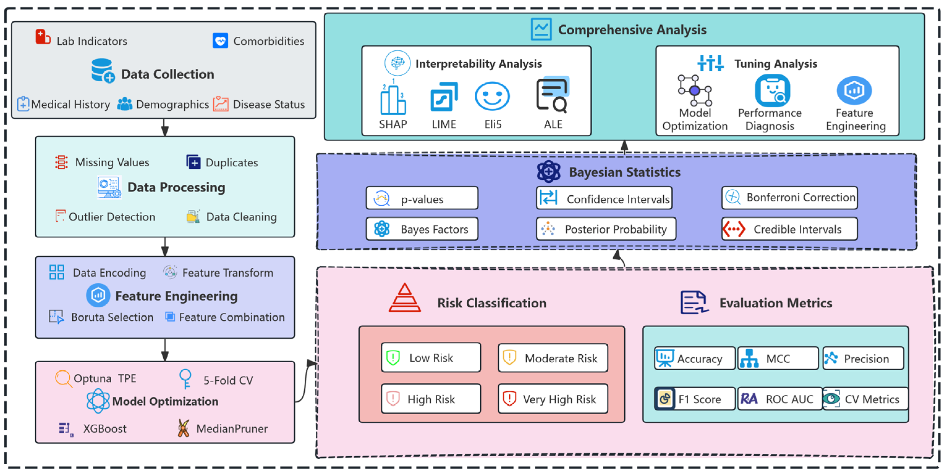
Figure 7 delineates the end-to-end computational pipeline for chronic kidney disease risk assessment. The workflow initiates with data acquisition encompassing patient demographics, comorbidities, laboratory biomarkers, medical histories, and disease status. Raw data undergoes systematic quality enhancement through missing value imputation, outlier detection, duplicate removal, and standardization protocols. Feature engineering applies encoding transformations, Boruta-based variable selection, and engineered feature combinations to optimize predictive signal. Model optimization leverages Optuna’s Tree-structured Parzen Estimator for XGBoost hyperparameter tuning with MedianPruner early stopping and 5-fold cross-validation to prevent overfitting. The trained classifier generates four-tier risk stratification evaluated through multiple performance metrics including accuracy, precision, F1-score, matthews correlation coefficient, and ROC-AUC. Statistical validation employs both frequentist approaches (p-values, confidence intervals, Bonferroni correction) and Bayesian inference (Bayes factors, posterior probabilities, credible intervals) to ensure robust significance assessment. The framework concludes with comprehensive analysis incorporating SHAP, LIME, Eli5, and ALE for model interpretability alongside performance diagnostics and feature engineering refinement, ensuring clinical transparency and decision support capability.

4.1. XGBoost

XGBoost employs an additive learning strategy wherein sequential weak learners progressively refine the ensemble’s predictive capacity. Each iteration introduces a new decision tree that minimizes the residual loss from preceding models. The algorithm’s strength lies in its regularized objective function, which simultaneously optimizes prediction accuracy and constrains model complexity through structural penalties:
L ϕ = i = 1 n ζ y i , y i ^ + k = 1 K Ω f k
where ζ denotes the differentiable loss function, Ω represents the complexity penalty incorporating both L 1 and L 2 regularization on leaf weights, and K is the total number of trees in the ensemble.

4.2. Boruta

Boruta implements a wrapper-based feature selection methodology that evaluates feature importance against randomized shadow attributes. The algorithm augments the original feature set with permuted copies and employs a random forest classifier to assess the statistical significance of each feature’s contribution. Features demonstrating consistently higher importance scores than their shadow counterparts are retained.
Z j = I m p X j μ s h a d o w σ s h a d o w
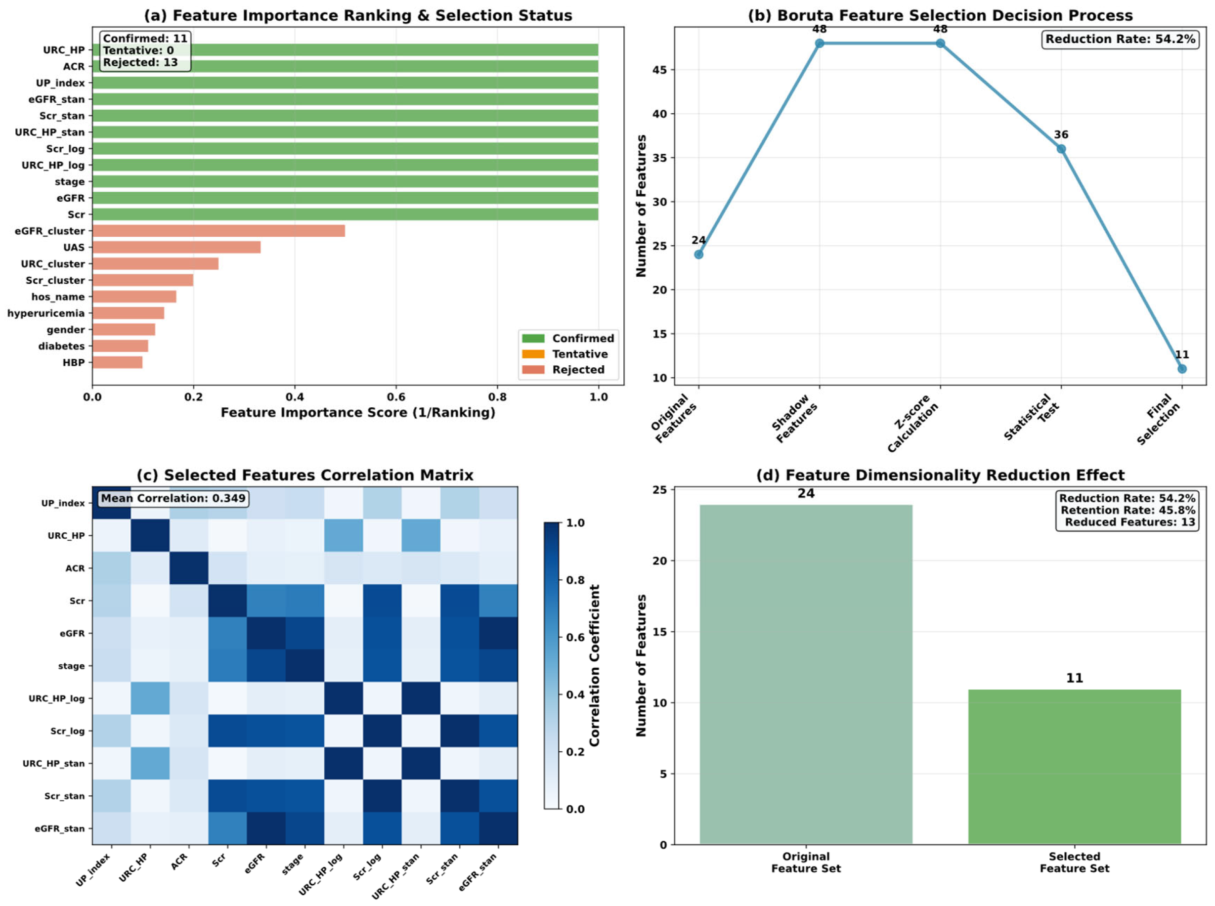
where I m p X j represents the importance measure for feature j , and μ s h a d o w and σ s h a d o w denote the mean and standard deviation of shadow feature importances, respectively. We implemented Boruta using the Python boruta package (v0.4.3) with RandomForestClassifier (n_estimators = 100, max_depth = 7, random_state = 42, class_weight = ‘balanced’) and Boruta-specific parameters (n_estimators = ‘auto’, max_iter = 100), converging at iteration 35 with 11 confirmed features.

4.3. Optuna

Optuna implements sequential model-based optimization through the Tree-structured Parzen Estimator, which constructs separate density models for promising and unpromising hyperparameter configurations. The algorithm partitions observed trials at a quantile threshold γ , modeling superior configurations with l x and inferior ones with g x . The expected improvement criterion drives the selection of subsequent trial parameters:
E I x = l x g x
This likelihood ratio focuses computational resources on hyperparameter regions demonstrating elevated potential for discovering optimal solutions. The iterative procedure systematically refines the search strategy by leveraging historical trial outcomes, as detailed in Algorithm 1.
Algorithm 1: Tree-structured Parzen Estimator
Input :   Objective   function   f ,   search   space   ,   trials   T ,   gamma   γ
1: Initialize   history   H
2: for   t   = 1   to   T   do
3:        Sort by objective values
4:         Split   trials   at   quantile   γ :   H g o o d ,   H p o o r
5:         Build   density   models :   l ( x ) p ( x H g o o d ) , g ( x ) p ( x H p o o r )
6:         Sample   candidates :   x i l ( x ) ,   i = 1 , . . . n
7:         Select :   x * a r g m a x x i l ( x i ) g ( x i ) *Acquisition function*
8:         Evaluate :   y * f ( x * )
9:         Update :   H H { ( x * , y * ) }
10:end for
11: return   best   configuration   from   H

4.4. Model Validation Strategy

The evaluation employs 5-fold cross-validation to rigorously assess model generalization while preserving class distribution across folds. The stratification mechanism ensures that each fold F k maintains proportional representation of all classes:
| F k c | | F k | = | D | | D |
where F k c denotes samples of class c in fold, k , D denotes all samples of class c in the dataset, and | · | indicates set cardinality.

5. Experiment

5.1. Experimental Configuration and Setup

All experiments were executed on a Windows 11 platform with 32 GB RAM, employing Python 3.11 as the core computational framework. The experimental framework integrated XGBoost 3.0.2 with Optuna 4.3.0 for Bayesian optimization and Boruta 0.4.3 for feature selection, as described in the methodology section. Consistent random seed initialization (seed = 42) was maintained across all computational processes to guarantee experimental reproducibility. Model evaluation employed stratified 5-fold cross-validation within the optimization loop, with the complete dataset partitioned using an 8:2 stratified train-test split to preserve class distribution across training and evaluation sets.

5.2. Performance Metrics

Classification performance was evaluated using multiple metrics tailored for multi-class risk stratification. Macro-averaging was prioritized to ensure balanced evaluation across imbalanced CKD risk categories.
Accuracy measures overall correct classification rate:
A c c u r a c y   = T P 1   +   T P 2   +   T P 3   +   T P 4 N  
Precision (macro-averaged) quantifies prediction reliability, reducing false alarms in clinical settings:
Precision macro = 1 4 c = 1 4 T P c T P c + F P c
Recall (macro-averaged) captures the model’s detection capability for each Risk Level, critical for preventing missed diagnoses:
Recall macro = 1 4 c = 1 4 T P c T P c + F N c
F1-Score (macro-averaged) harmonizes precision and recall through their harmonic mean:
F 1 macro = 1 4 c = 1 4 2 × Precision c × Recall c Precision c + Recall c
ROC AUC (One-vs-Rest) evaluates class separability using pairwise comparisons:
AUC   OvR = 1 4 c = 1 4 AUC c
MCC (Matthews Correlation Coefficient) offers robust quality assessment for imbalanced datasets:
MCC = T P × T N F P × F N T P + F P T P + F N T N + F P T N + F N
Cohen’s Kappa measures agreement beyond random chance, adjusting for baseline prevalence:
κ = p o p e 1 p e
Paired t-test assessed performance differences when normality assumptions were satisfied:
t = d ¯ s d / n
Wilcoxon signed-rank test provided non-parametric assessment for non-normal distributions:
W = i = 1 n rank d i I d i > 0
Confidence Interval quantified estimation uncertainty through parametric bounds:
CI α = d ¯ ± t α / 2 , n 1 s d n
Bonferroni correction controled family-wise error rate across multiple comparisons:
α corrected = α k
where α = 0.05 and k represents the number of pairwise comparisons.
Bayes Factor quantified relative evidence supporting model superiority using the Savage–Dickey density ratio:
BF 10 = p θ = 0 prior p θ = 0 posterior
where BF 10 > 10 indicates strong evidence for the alternative hypothesis.
Posterior Probability-derived model selection confidence from Bayes factors:
P H 1 data = BF 10 1 + BF 10
assuming equal prior probabilities for competing hypotheses.
Predictive Probability assessed superiority likelihood exceeding clinical thresholds:
P Δ > τ data = τ p Δ data d Δ
where τ represents the minimum clinically meaningful performance difference and Δ denotes the performance gap between models.

5.3. Model Performance Comparison and Analysis

Table 2 displays the performance evaluation of our framework against 20 baseline algorithms. Our method achieved F1-score of 93.1%, accuracy of 93.4%, and ROC-AUC of 97.6%, demonstrating substantial improvements over all baseline approaches. The cross-validation mean of 88.4% with standard deviation of 0.018 indicates robust generalization across diverse data partitions. Among baseline algorithms, standard XGBoost exhibited the strongest performance (F1: 86.9%, Accuracy: 87.9%), followed by LightGBM (F1: 86.1%) and CatBoost (F1: 84.5%). Ensemble strategies including Voting Classifier (F1: 84.9%) and Stacking (F1: 83.9%) achieved competitive results, though remained substantially below our optimized approach. Traditional gradient boosting methods showed moderate effectiveness, with GBDT attaining 83.9% F1-score and AdaBoost reaching 81.7%. Linear models demonstrated acceptable performance, with Logistic Regression (F1: 81.3%), ElasticNet (F1: 81.3%), and Lasso (F1: 80.9%) achieving comparable results. However, Ridge Classifier exhibited limited effectiveness (F1: 62.2%), while distance-based methods revealed notable constraints, with KNeighbors reaching an 82.9% F1-score. The MLP achieved 73.4% F1-score, and probabilistic methods showed considerable limitations, with GaussianNB attaining only 73.1% and Perceptron demonstrating the poorest performance at 66.6% F1-score. MCC for our approach reached 0.903, substantially exceeding the best baseline (XGBoost: 0.820), confirming superior classification quality even under class imbalance.
Table 3 presents a comprehensive comparison of various models through Bayesian-Frequentist dual validation, highlighting the robustness and performance of our method across multiple metrics. Our model achieved an impressive F1 score of 85.0% ± 2.5%, outperforming 20 baseline models. Among the baselines, Stacking showed the strongest performance with an F1 score of 83.1% ± 3.0%, followed closely by Lasso (82.8% ± 2.4%) and ElasticNet (82.4% ± 2.2%).
Gradient boosting methods like XGBoost and LightGBM demonstrated competitive results, with F1 scores of 79.4% ± 3.6% and 79.3% ± 3.8%, respectively, indicating moderate stability. Interestingly, Ridge and Perceptron models resulted in a zero ROC-AUC, attributed to their lack of probabilistic output capabilities.
GaussianNB showed extreme instability, reflected in its low F1 score of 45.0% ± 9.7%. Traditional tree-based methods such as Random Forest, Decision Tree, and Extra Trees consistently underperformed compared to other models. MCC further confirmed the superiority of our approach, with our model achieving an MCC of 0.793% ± 0.034%, surpassing Stacking’s 0.776% ± 0.041%. This validates the convergence of evidence from both frequentist and Bayesian perspectives, reinforcing the robustness of our model.
Table 4 provides a detailed cross-validation analysis of various models, highlighting the exceptional stability of our method with a CV standard deviation of 0.012. This stability surpasses that of the baseline models, which range from 0.009 to 0.051. The dual statistical frameworks employed demonstrate convergent evidence: frequentist testing confirmed significance (p < 0.001) across all 20 comparisons, while Bayesian credible intervals closely matched the confidence intervals, validating inference consistency. Effect sizes varied significantly, from 0.665 for Stacking to 9.707 for Ridge. Gradient boosting methods such as XGBoost and LightGBM exhibited moderate-to-large effects, with effect sizes of 1.795 and 1.749, respectively. Notably, GaussianNB showed extreme variability with a CV standard deviation of 0.051, whereas Stacking maintained the strongest baseline stability with a CV standard deviation of 0.011. The convergence of the 95% confidence intervals and credible intervals (mean difference <0.001) confirmed robust statistical consensus across paradigms, reinforcing the reliability and effectiveness of our method compared to the baseline models.
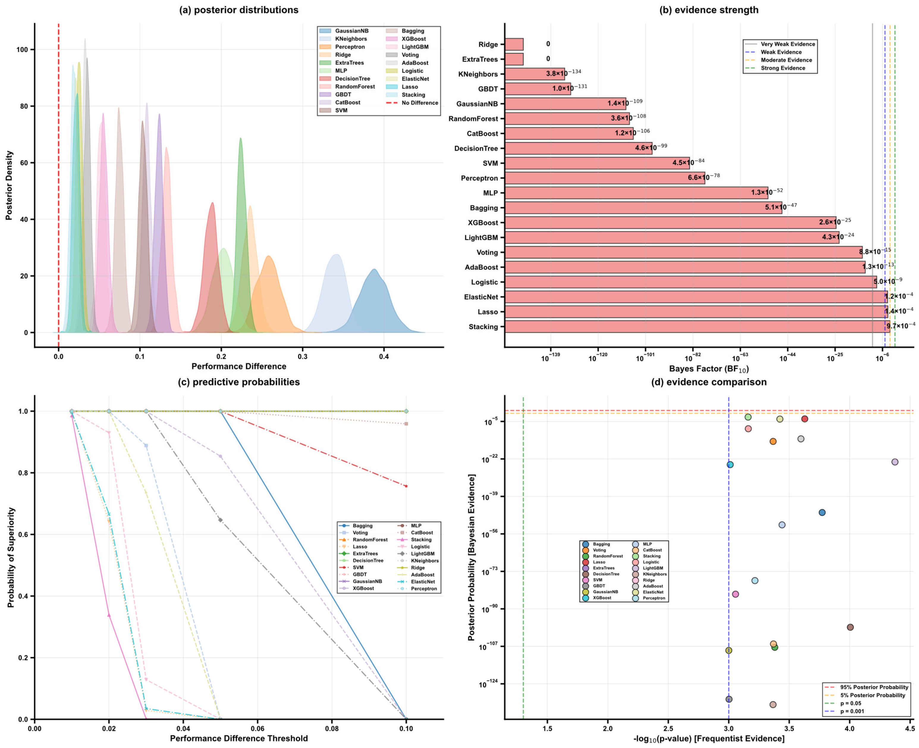
Figure 8 presents a four-panel Bayesian inference synthesis comparing baseline models against our method. Panel (a) depicts posterior probability distributions of performance differences, revealing substantial heterogeneity across models. GaussianNB exhibits the rightmost distribution peak (mean difference ≈ 0.39), indicating marked underperformance, while ensemble methods (Stacking, Lasso, ElasticNet) cluster near zero-difference baseline with posterior means below 0.025, suggesting performance equivalence. The bimodal separation between high-variance estimators (KNeighbors, Perceptron, RidgeClassifier with means 0.23–0.34) and regularized approaches reflects fundamental bias-variance tradeoffs. All distributions reside exclusively in positive territory beyond the red reference line, confirming systematic performance deficits.
Panel (b) quantifies evidence strength through Bayes Factor (BF10) magnitudes spanning 150 orders of magnitude, from decisive evidence against alternative hypotheses (ExtraTrees, Ridge: BF10 ≈ 10−150) to approaching moderate levels (Stacking: BF10 = 9.7 × 10⁻⁴). Reference thresholds partition the evidence landscape: 17 models fall below 10−10 (very weak evidence), while only three regularized models (ElasticNet, Lasso, Stacking) exceed 10−4, approaching but not surpassing the 10−3 threshold for moderate evidence.
Panel (c) tracks predictive probability trajectories across performance thresholds from 0.01 to 0.10, stratifying models into three archetypes: rapid probability decay (Stacking, ElasticNet, Lasso reaching near-zero by 0.03 threshold), intermediate descent (ensemble boosting methods maintaining 0.2–0.4 probability at 0.05), and sustained elevation (GaussianNB, KNeighbors retaining probabilities above 0.6 throughout).
Panel (d) juxtaposes Bayesian posterior probabilities against frequentist p-value evidence on dual logarithmic axes. The scatter distribution reveals weak positive correlation with substantial vertical dispersion, indicating that equivalent frequentist significance levels (-log10(p) = 3–4) translate into highly variable Bayesian evidence (10−15 to 10−2). The concentration of points in the lower-left quadrant demonstrates the anti-conservative bias of p-values, where statistically significant results may carry negligible posterior probability of hypothesis truth.
Table 5 presents the hyperparameter search spaces employed by various hyperparameter optimization methods. The comparison encompasses 20 optimization approaches, including our proposed method alongside established techniques such as Bayesian optimization (BOHB, Hyperopt, Scikit-Optimize), evolutionary algorithms (Genetic Algorithm, Differential Evolution, CMA-ES), early-stopping strategies (ASHA, Hyperband, Successive Halving, PBT), AutoML frameworks (Auto-sklearn, FLAML, H2O AutoML), and bandit-based methods (MAB, Thompson Sampling, UCB). The search spaces are defined across five key XGBoost hyperparameters: n_estimators (number of boosting rounds), max_depth (maximum tree depth), learning_rate (step size shrinkage), subsample (fraction of samples for tree building), and colsample_bytree (fraction of features for tree building). Our method specifies n_estimators in the range (200, 2000), max_depth in (3, 15), learning_rate with logarithmic scaling log(0.005–0.3), and both subsample and colsample_bytree in (0.5, 1.0). Parentheses denote continuous ranges, while square brackets indicate discrete or uniformly sampled intervals.
Table 6 presents a comprehensive evaluation of 20 hyperparameter optimization methods. Our proposed method achieved the highest classification performance (Accuracy: 0.9343, F1: 0.9313, MCC: 0.9028, ROC AUC: 0.9759) with 50 evaluations, outperforming all baseline approaches. Random Search demonstrated competitive results (Accuracy: 0.9293, F1: 0.9227, MCC: 0.8953) with identical computational budget, validating its effectiveness as a simple yet robust optimization strategy. PBT achieved F1: 0.9180 while exhibiting the lowest cross-validation variance (CV_Std: 0.0065), indicating superior model stability across different data partitions. Scikit-Optimize achieved F1: 0.9150 with the smallest generalization gap (−0.0394) among top-performing methods, suggesting optimal training–validation balance. The computational efficiency varied substantially across methods: Grid Search required 540 evaluations (F1: 0.9020), FLAML consumed 1069 evaluations (F1: 0.9015) representing a 21-fold increase compared to our method, while H2O AutoML utilized only 16 evaluations, achieving F1: 0.8963 with exceptional cross-validation stability (CV_Mean: 0.9608, CV_Std: 0.0062). Bayesian optimization variants showed moderate performance, with Hyperopt (F1: 0.9020, 50 evaluations) outperforming BOHB (F1: 0.8758, 50 evaluations) by 2.6 percentage points despite identical evaluation budgets. Evolutionary strategies demonstrated variable results: Genetic Algorithm (F1: 0.8984, 56 evaluations), PSO (F1: 0.8976, 60 evaluations), Differential Evolution (F1: 0.8863, 60 evaluations), and CMA-ES (F1: 0.8758, 50 evaluations). Early-stopping strategies maintained computational efficiency: Successive Halving (F1: 0.9083, 72 evaluations) achieved the best performance within this category, surpassing ASHA (F1: 0.8882, 50 evaluations) and Hyperband (F1: 0.8860, 50 evaluations). Bandit-based methods exhibited performance divergence: UCB achieved competitive results (F1: 0.9084, MCC: 0.8805), while MAB and Thompson Sampling showed identical performance (F1: 0.8714, MCC: 0.8281).
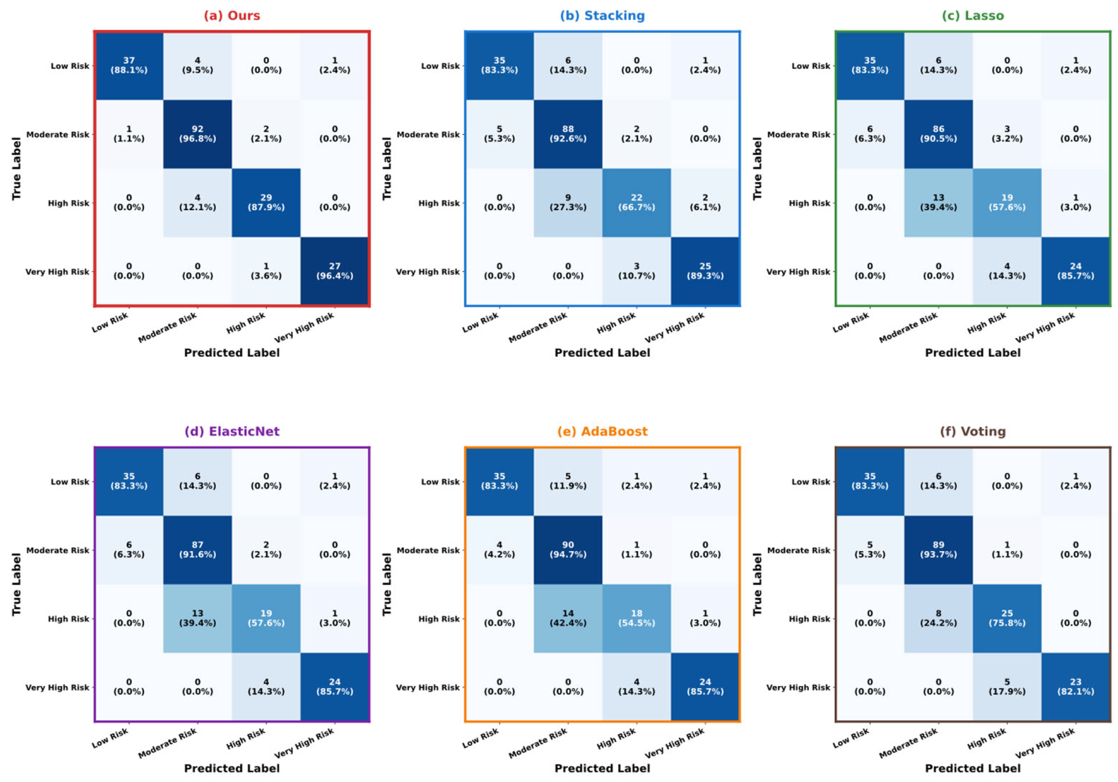
Figure 9 presents classification outcome matrices for six competing approaches, comparing predictive performance across the four-tier CKD risk stratification framework. Matrix rows represent actual patient classifications, while columns display algorithm predictions, with numerical entries denoting patient counts and diagonal values expressing category-specific correct classification rates. Our framework achieves pronounced diagonal concentration, attaining 88.7% (Low Risk), 96.8% (Moderate Risk), 87.9% (High Risk), and 96.4% (Very High Risk) accuracy, demonstrating robust discriminative capability. Classification errors predominantly manifest between neighboring severity tiers, consistent with inherent clinical ambiguity in transitional patient profiles. Comparative analysis reveals our approach sustains tighter prediction clustering along the principal diagonal, minimizing cross-category misattribution relative to ensemble alternatives such as AdaBoost and Voting, which display elevated error rates between proximate risk strata. The marked performance advantage in critical severity detection (96.4% vs. 82.1% for Voting, 85.7% for Stacking) underscores clinical value for prioritizing patients necessitating urgent therapeutic escalation, while preserving equitable detection sensitivity across the complete risk spectrum vital for holistic CKD patient management.
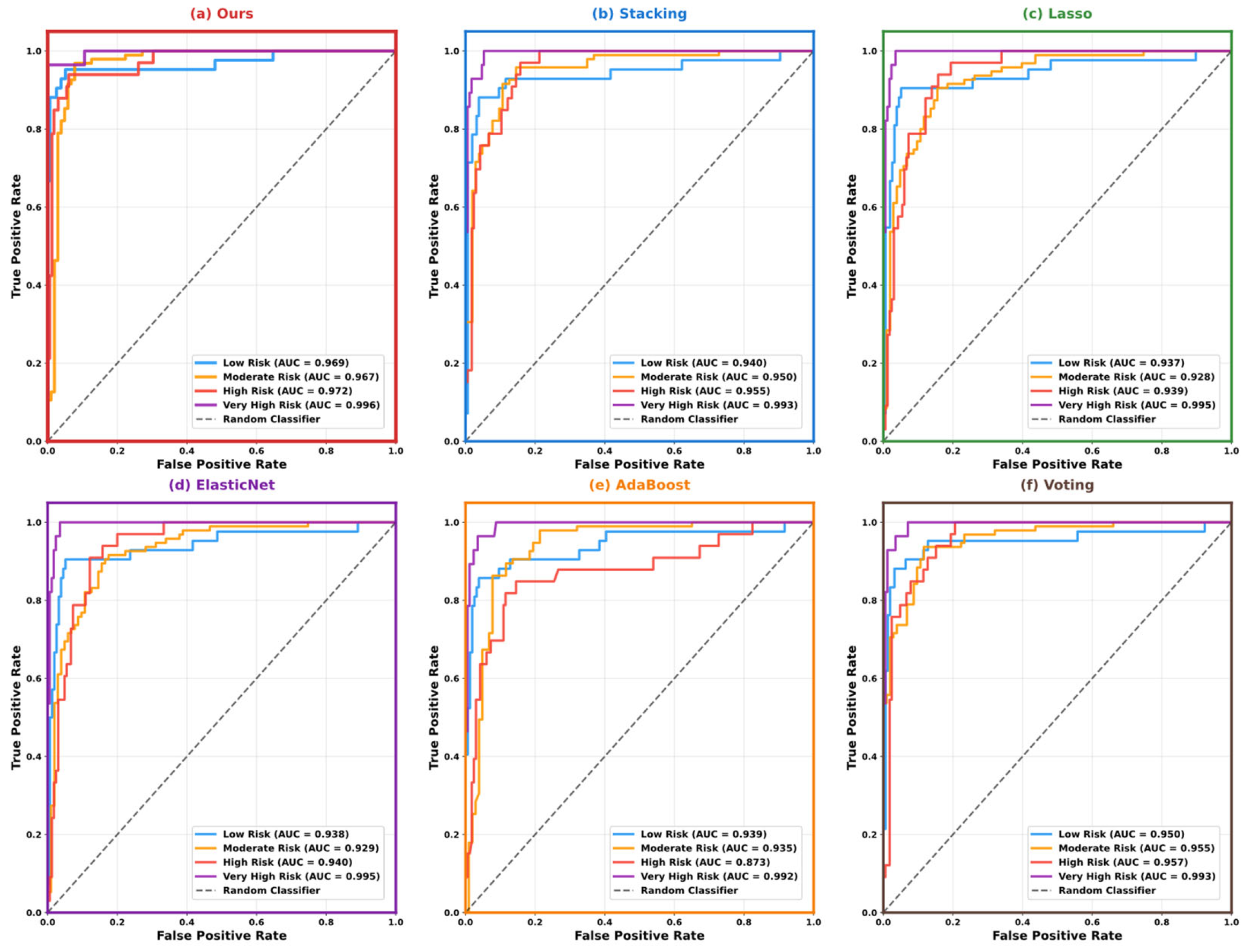
Figure 10 illustrates receiver operating characteristic trajectories across the quaternary CKD severity framework, with area-under-curve measurements quantifying class discrimination capability. Our framework sustains uniformly strong separability indices spanning all severity tiers: Low Risk (0.969), Moderate Risk (0.967), High Risk (0.972), and Very High Risk (0.996), establishing enhanced inter-category distinction relative to comparison methodologies. Benchmarking analysis exposes performance deterioration among conventional ensemble architectures, notably manifested in AdaBoost’s High Risk discrimination (AUC = 0.873). The characteristic upper-left quadrant approximation in our curves signifies optimal balance between sensitivity and specificity dimensions, capturing elevated true-positive identification while constraining false-positive incidence across threshold variations. Severity-stratified evaluation reveals remarkable discriminative capacity for critical patient identification (AUC = 0.996 vs. 0.994 for Stacking), paramount for clinical triage of individuals necessitating immediate therapeutic escalation.
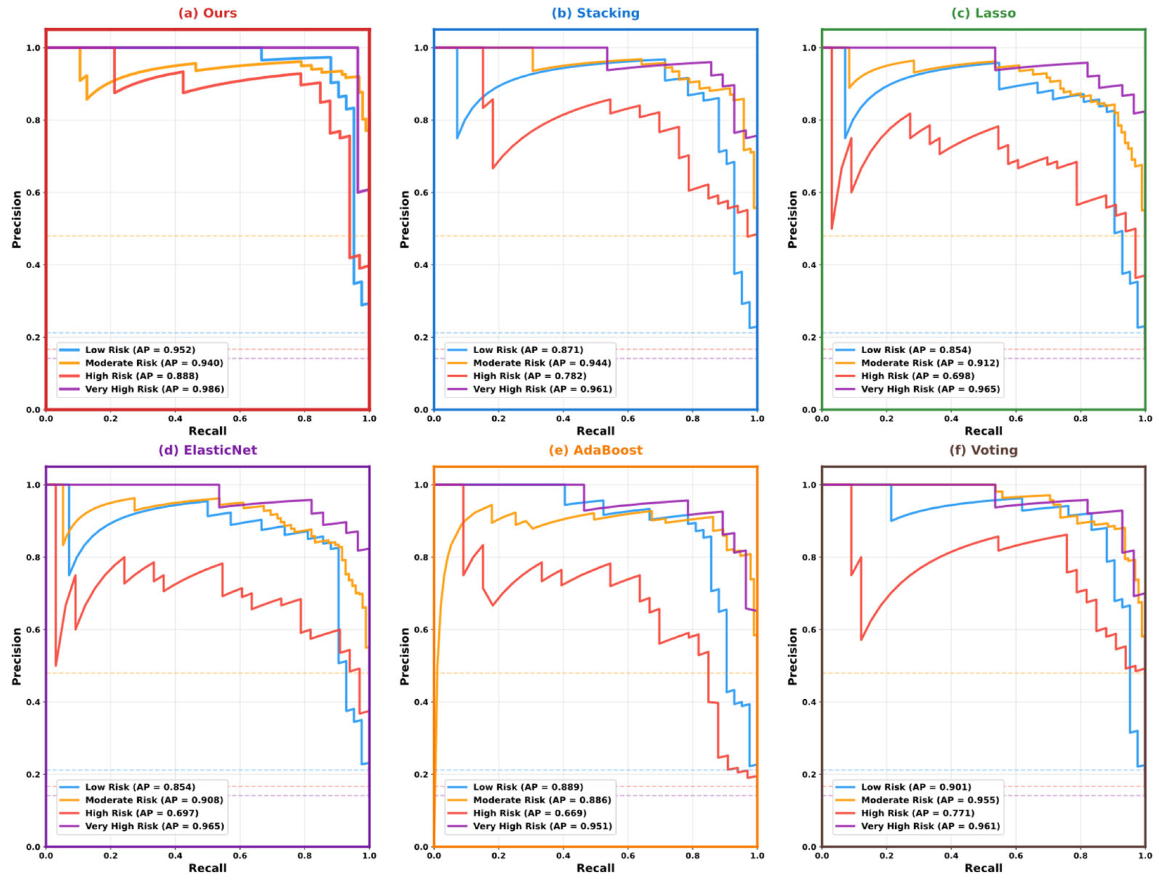
Figure 11 visualizes the positive predictive value versus sensitivity balance throughout the quaternary CKD severity classification framework, with mean average precision indices characterizing algorithmic performance across operational threshold variations. Our framework exhibits consistent positive predictive stability spanning sensitivity continuum endpoints, registering mean precision scores of 0.952 (Low Risk), 0.940 (Moderate Risk), 0.888 (High Risk), and 0.986 (Very High Risk), signifying resilient affirmative prediction capability throughout severity categories. Benchmarking evaluation exposes marked performance heterogeneity under distributional asymmetry conditions, wherein comparison methodologies manifest considerable positive predictive deterioration at elevated sensitivity operating points, notably exemplified in Stacking’s High Risk trajectory (AP = 0.782) and Lasso’s Low Risk discrimination (AP = 0.854). The characteristic sustained elevation in our curves signifies preserved classification certainty despite threshold mobility, diverging from the systematic positive predictive erosion characteristic of conventional ensemble architectures. Severity-stratified assessment demonstrates remarkable consistency, exhibiting minimal positive predictive variance throughout sensitivity range for critical severity identification (AP = 0.986), whereas comparison approaches demonstrate accelerated positive predictive decline exceeding 0.6 sensitivity threshold.
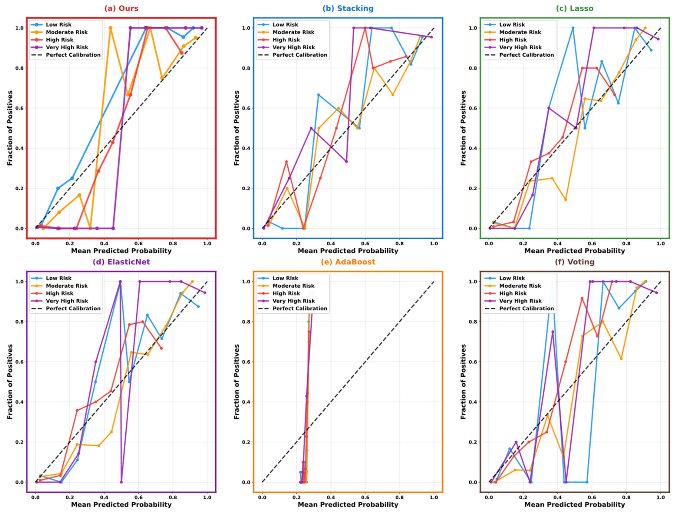
Figure 12 displays reliability diagrams examining concordance between algorithm-generated probability estimates and empirical event frequencies throughout the quaternary CKD severity framework, where unity-slope reference trajectories represent ideal probabilistic accuracy. Our framework registers weighted MAE = 0.160, establishing competitive reliability metrics spanning severity classifications, with notable proficiency in Low Risk probability estimation (MAE = 0.127). Cross-algorithmic evaluation exposes heterogeneous reliability profiles: Lasso (weighted MAE = 0.115), ElasticNet (weighted MAE = 0.119), and Stacking (weighted MAE = 0.134) demonstrate reduced aggregate deviation indices, albeit exhibiting category-specific performance asymmetries. Our implementation sustains uniform intermediate-fidelity probability alignment throughout all severity tiers, circumventing catastrophic reliability failures evident in alternative approaches. Critically, AdaBoost manifests profound reliability degradation (weighted MAE = 0.320), with Moderate Risk deviation surpassing 0.39, compromising confidence quantification integrity despite preserved discrimination metrics (ROC-AUC). These observations underscore that discrimination excellence and probability fidelity constitute orthogonal performance dimensions, reinforcing comprehensive evaluation imperatives in clinical prediction contexts.
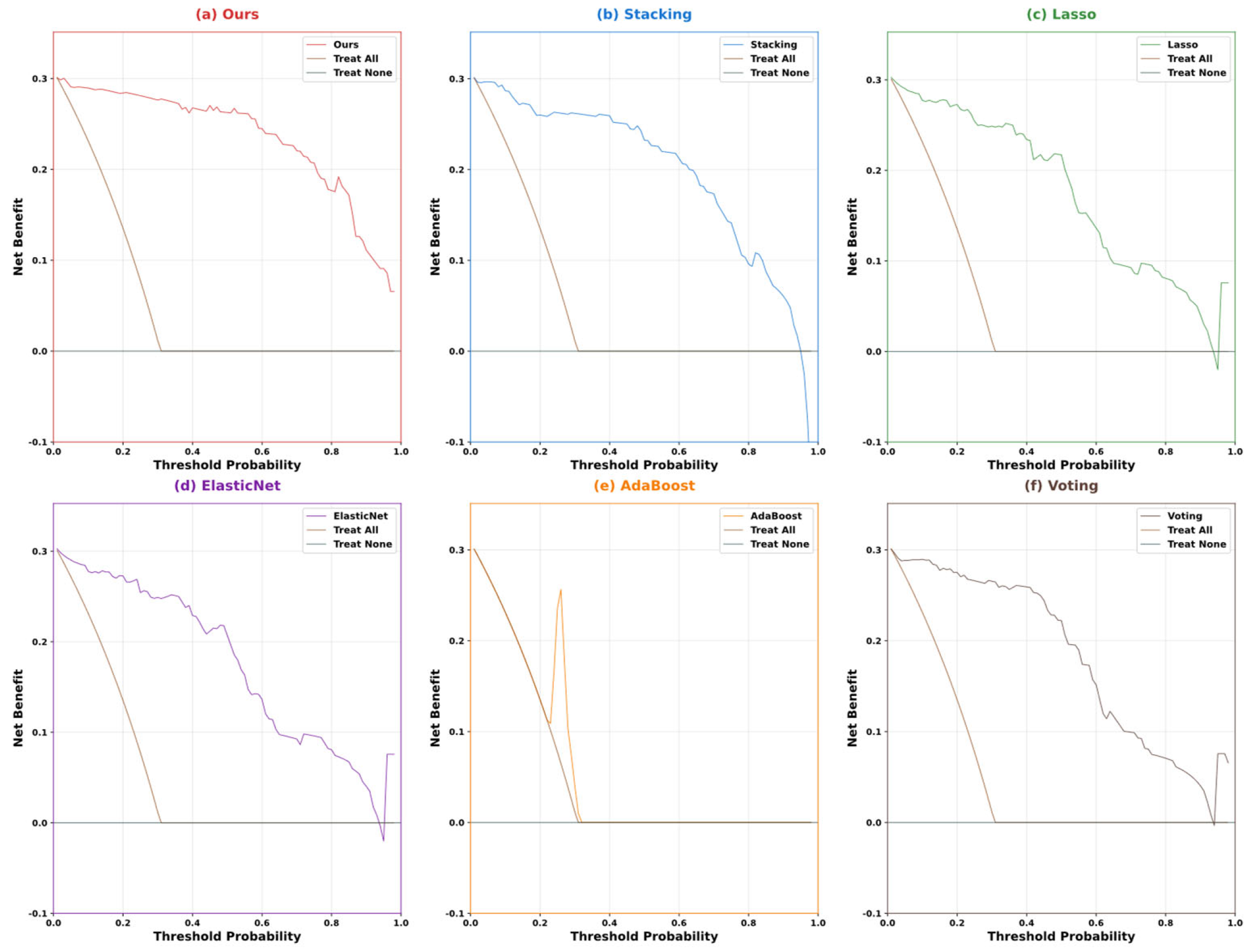
Figure 13 illustrates intervention value assessment examining therapeutic gain throughout probability thresholds spanning 0.0 to 1.0, contrasting algorithm-directed triage protocols with universal-treatment and observation-only reference standards. Our framework attains peak therapeutic gain of 0.301 at 0.01 probability cutoff, converging with leading comparison methodologies (Lasso: 0.303, ElasticNet: 0.303, Stacking: 0.301), while sustaining affirmative intervention value throughout an extensive threshold continuum (0.01–0.98). The trajectory uniformly supersedes both benchmark strategies, preserving positive therapeutic gain extending to 0.98 probability boundary. Cross-methodological assessment exposes that Lasso, ElasticNet, Ours, and Voting sustain comparable expansive utility domains (0.94–0.98), whereas AdaBoost demonstrates markedly constrained applicability (0.31) accompanied by unstable oscillations, compromising threshold-contingent clinical determinations. The convergent peak performance among diverse approaches (0.301–0.303, < 1% variance) establishes that intervention value at optimal operational thresholds derives principally from accurate severity stratification rather than algorithmic architecture selection, while persistent advantage relative to universal-treatment baseline substantiates individualized therapeutic targeting.
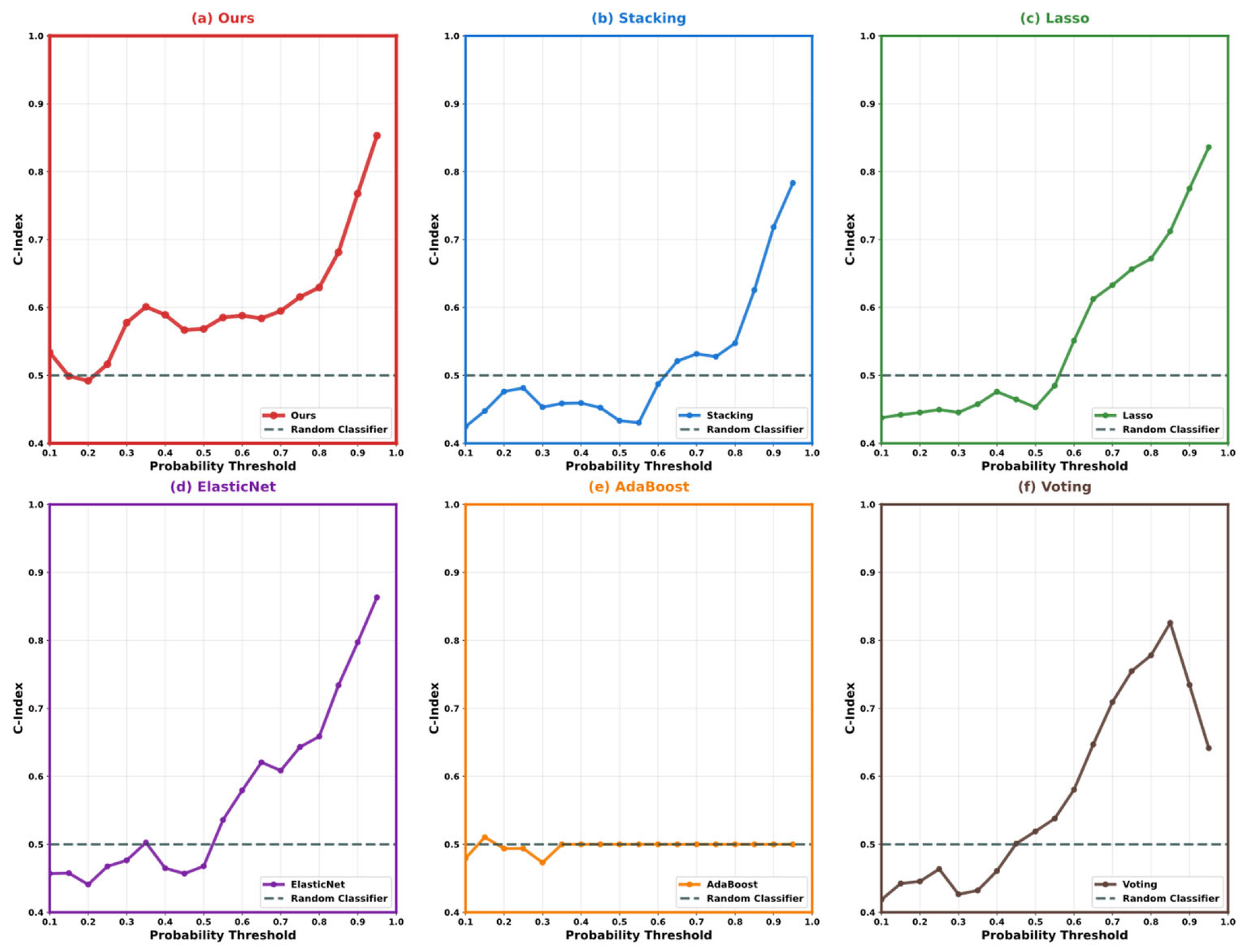
Figure 14 illustrates concordance index evolution throughout probability cutoffs spanning 0.1 to 1.0, characterizing ordinal ranking proficiency through dyadic observation comparisons. Our framework preserves consistent concordance metrics ranging 0.50–0.60 throughout 0.1–0.8 probability spectrum, featuring distinctive elevation maxima proximal to 0.3–0.4 intervals (concordance ≈ 0.61), succeeded by precipitous escalation reaching 0.85 at 0.95 cutoff, establishing resilient discriminative uniformity across cautious-to-liberal classification paradigms. Cross-algorithmic evaluation exposes heterogeneous threshold-contingent dynamics, wherein Stacking manifests sustained baseline concordance (≈0.50) extending through 0.6 probability demarcation preceding ascension to 0.78, whereas Lasso exhibits progressive monotonic enhancement from 0.40 to 0.84 throughout complete threshold continuum. ElasticNet replicates analogous trajectory with protracted plateau at 0.50 persisting until 0.5 demarcation, subsequently advancing to 0.86, signifying threshold-modulated discrimination emergence. Critically, AdaBoost demonstrates aberrant horizontal persistence sustaining concordance ≈ 0.50 (stochastic classifier equivalence) throughout entire probability range, substantiating profound ordinal sequencing deficiencies concordant with antecedent calibration inadequacies. Voting exhibits postponed discrimination initiation with concordance approximating 0.42 through 0.5 probability boundary, succeeded by abrupt enhancement to 0.82 accompanied by terminal instability at 0.65 cutoff. The horizontal dashed reference trajectory at 0.5 denotes stochastic classifier benchmark, with all methodologies excluding AdaBoost ultimately transcending this demarcation, corroborating discriminative proficiency despite heterogeneous threshold dependencies relevant to deployment contexts.

5.4. Model Interpretability Analysis

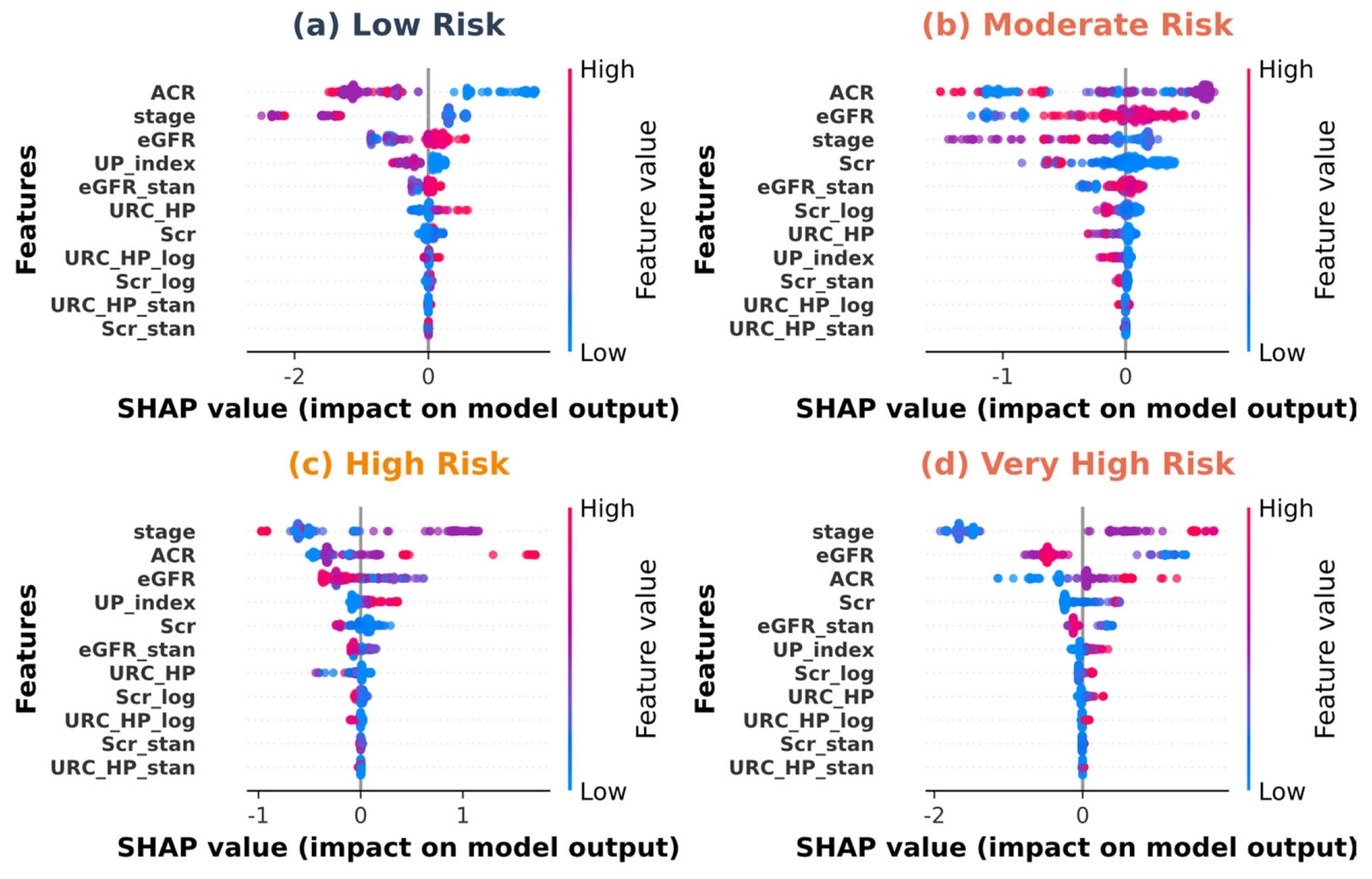
Figure 15 presents feature-specific SHAP value distributions for model predictions across four CKD risk strata. (a) Low Risk patients exhibit dominant positive contributions from ACR (SHAP ≈ +2.0) and stage indicators, while eGFR and standardized metrics show protective negative influences (SHAP ≈ −1.5 to −0.5), reflecting preserved renal function profiles. (b) Moderate Risk cases demonstrate balanced contribution patterns with ACR maintaining moderate positive impact (SHAP ≈ +1.0) alongside distributed influences from eGFR_stan and UP_index, indicating intermediate pathophysiological states. (c) High Risk patients display pronounced stage effects (SHAP ≈ +1.5) combined with sustained ACR contributions, while eGFR exhibits bidirectional impacts spanning −1 to +1, suggesting advanced dysfunction with variable compensatory mechanisms. (d) Very High Risk individuals show the most dramatic SHAP value dispersion, with stage and eGFR_cluster generating strong positive contributions (SHAP ≈ +2.0), ACR demonstrating elevated influence, and protective factors largely absent, consistent with severe multi-parameter deterioration characteristic of end-stage pathology.
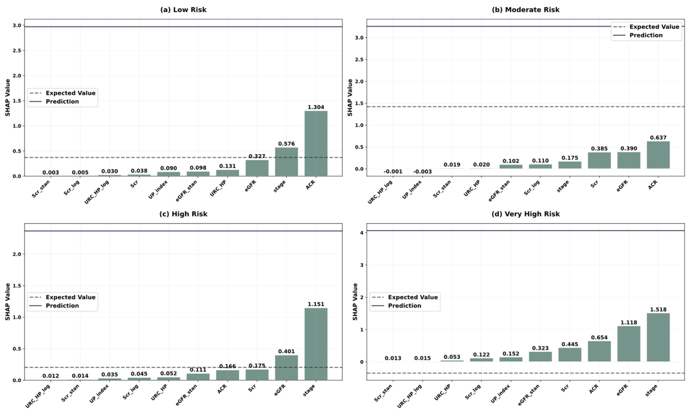
Figure 16 illustrates patient-specific prediction decomposition through waterfall plots depicting cumulative feature contributions. (a) Low Risk classification (final prediction 1.304) originates from expected value baseline (0.257), with ACR providing dominant positive contribution (+0.576) while UP_index, Scr_log, and eGFR exert modest influences (+0.030 to +0.131), demonstrating relatively simple decision pathways in preserved renal function. (b) Moderate Risk prediction (0.637) emerges through distributed contributions where ACR (+0.385), stage (+0.175), and Scr (+0.110) accumulate incrementally from baseline (−0.001), reflecting multifactorial intermediate disease states. (c) High Risk assignment (1.151) displays pronounced stage influence (+0.401) alongside ACR contribution (+0.275) from expected value baseline (0.012), with supporting effects from eGFR_stan and UP_index, indicating advanced pathophysiological integration. (d) Very High Risk classification (1.518) exhibits the steepest cumulative trajectory, where stage provides substantial positive drive (+1.118) followed by ACR (+0.645) and eGFR contributions (+0.223), with baseline expectation at 0.013, demonstrating extreme deviation toward maximal risk prediction through synergistic biomarker deterioration.
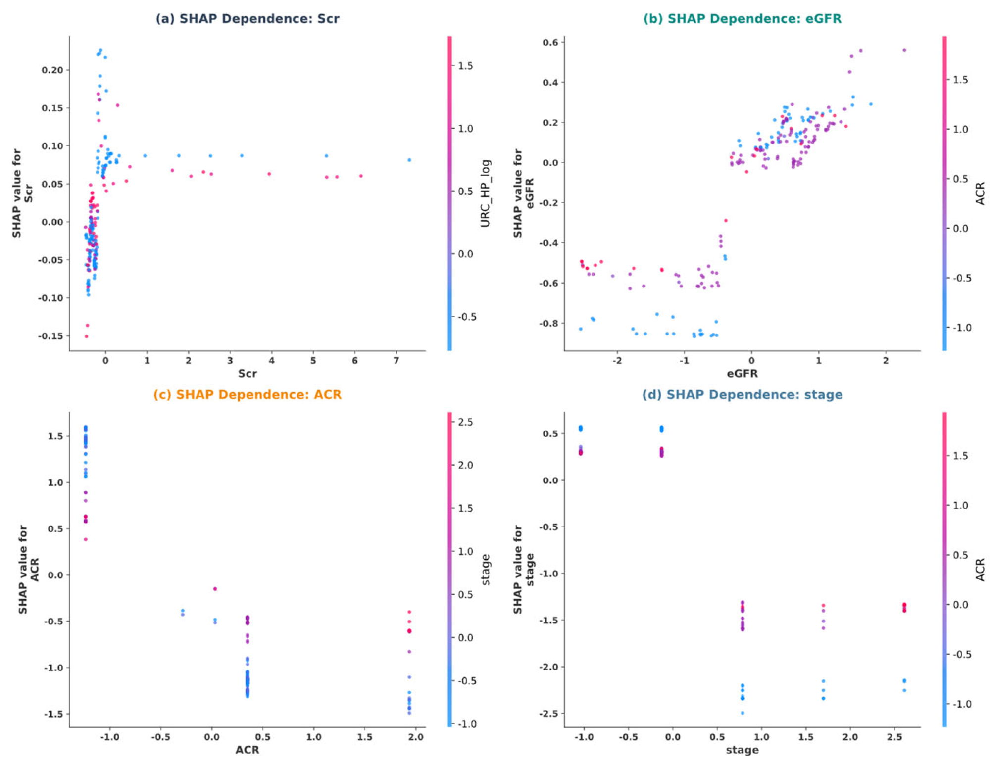
Figure 17 describes SHAP dependence plots illustrating the relationship between key clinical features and their marginal contribution to CKD risk prediction. Panel (a) depicts serum creatinine (Scr, range 0–7) showing concentrated negative impacts (SHAP ≈ −0.10) at baseline values with diminishing influence at elevated concentrations. Panel (b) presents eGFR (standardized values −2 to +2) exhibiting an inverse association where preserved renal function yields protective contributions (SHAP < −0.6) while impaired filtration drives risk escalation (SHAP up to +0.6), with interaction strength encoded by color intensity. Panel (c) demonstrates ACR (range −1.0 to +2.0) displaying progressive risk amplification (SHAP values spanning −1.5 to +1.5) correlating with albuminuria severity, characterized by sharp inflection points at pathological thresholds. Panel (d) reveals stage-wise stratification across CKD stages (−1.0 to +2.5) with discrete SHAP value distributions (ranging −2.5 to +0.5) corresponding to clinical severity levels, where interaction patterns highlight synergistic effects with concurrent biomarkers.
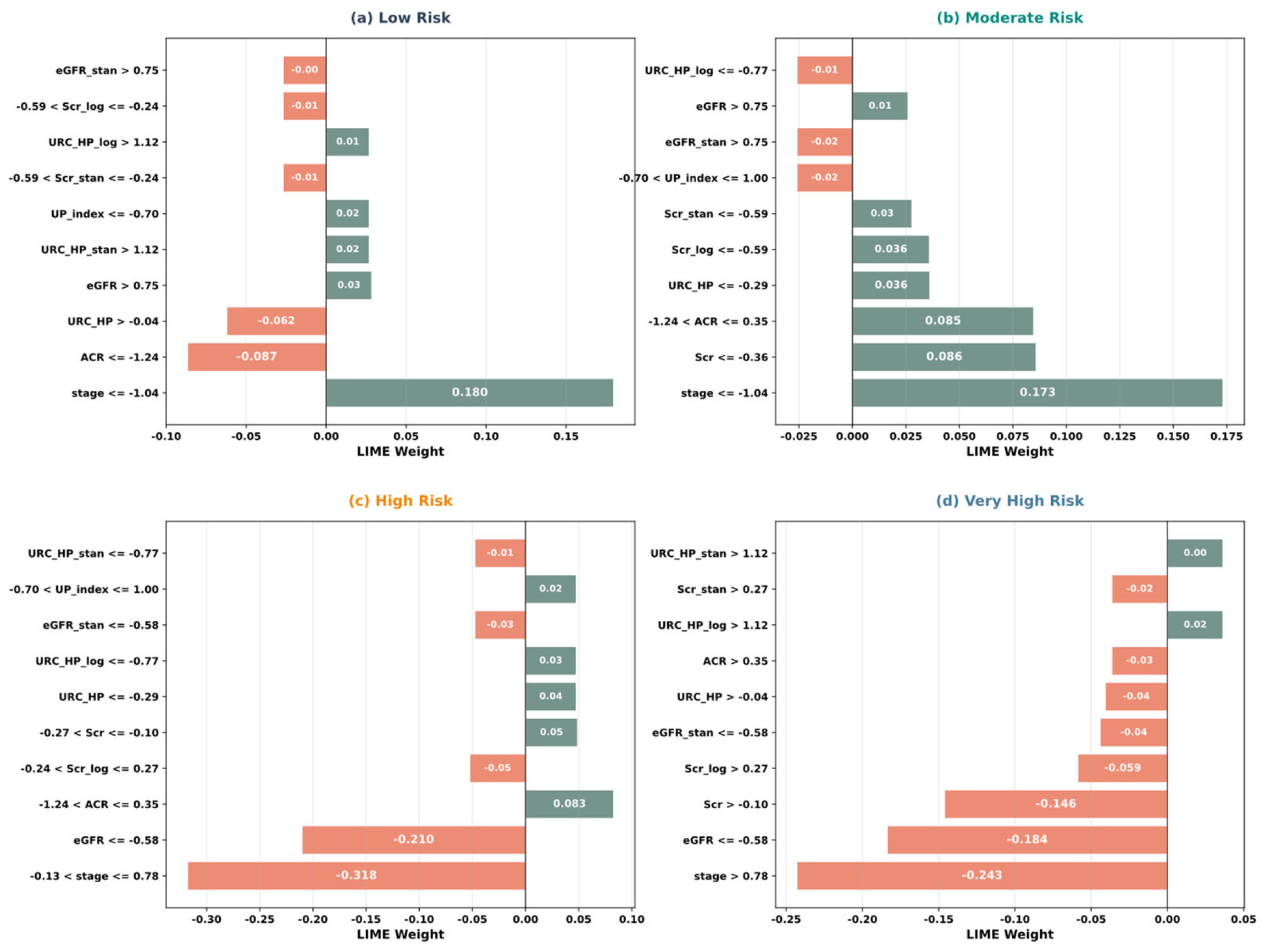
Figure 18 describes LIME-derived feature importance weights illustrating individualized prediction explanations across CKD risk strata. Panel (a) Low Risk classification demonstrates protective contributions from preserved renal markers (stage ≤−1.04, weight = +0.180) alongside modest positive inputs from maintained eGFR and controlled proteinuria levels (weights ranging +0.01 to +0.05). Panel (b) Moderate Risk profile exhibits balanced feature interplay with stage progression (≤−1.04, weight = +0.173) and elevated Scr (≤−0.36, weight = +0.086) driving risk attribution, while compensatory eGFR maintenance provides opposing influence (weight = +0.01). Panel (c) High Risk determination reflects pronounced negative contributions from advanced disease stage (−0.13 ≤ stage ≤ −0.78, weight = −0.318) and compromised filtration (eGFR ≤ −0.58, weight = −0.210), with minor offsetting effects from specific biomarker thresholds. Panel (d) Very High Risk categorization shows dominant negative weights from critical stage deterioration (>0.78, weight = −0.243) and severely reduced eGFR (≤−0.58, weight = −0.184), alongside substantial contributions from elevated Scr (>−0.10, weight = −0.146) and pathological proteinuria patterns.
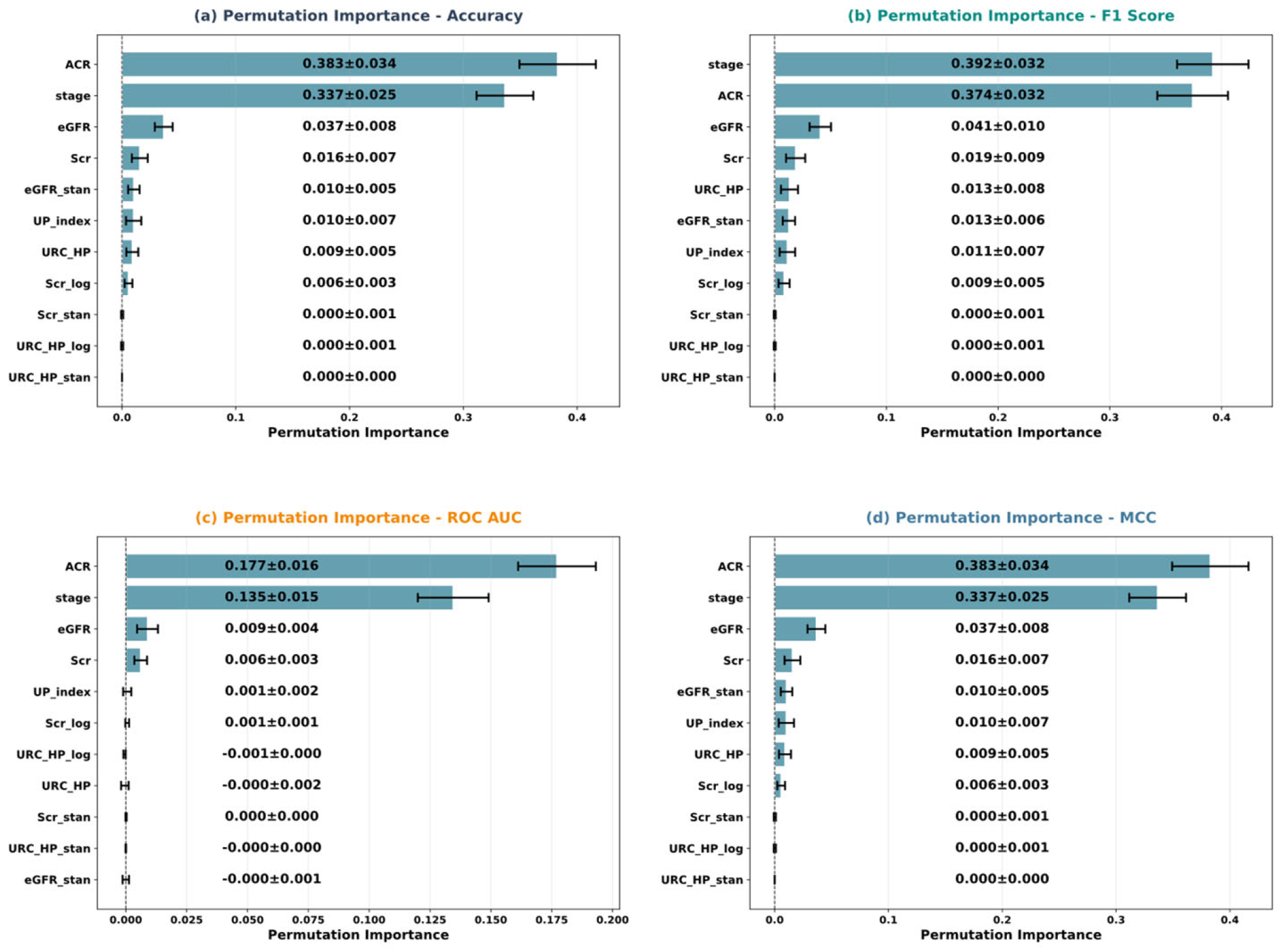
Figure 19 shows permutation importance scores quantifying feature contributions to predictive performance across multiple evaluation metrics, with error bars representing standard deviations from 30 bootstrap iterations. Panel (a) accuracy-based assessment identifies ACR (0.383 ± 0.034) and stage (0.337 ± 0.025) as dominant predictors, with eGFR exhibiting minimal contribution (0.037 ± 0.008). Panel (b) F1-weighted evaluation reveals comparable primacy of stage (0.392 ± 0.032) and ACR (0.374 ± 0.032), while eGFR maintains modest influence (0.041 ± 0.010). Panel (c) ROC AUC metric demonstrates ACR supremacy (0.177 ± 0.016) followed by stage (0.135 ± 0.015), with substantially attenuated eGFR impact (0.009 ± 0.004). Panel (d) MCC confirms the ACR-stage dominance pattern (0.383 ± 0.034 and 0.337 ± 0.025, respectively), with eGFR contribution at 0.037 ± 0.008. The consistent feature hierarchy across diverse metrics validates ACR and disease stage as primary determinants of CKD risk stratification, while highlighting the differential sensitivity of evaluation criteria to biomarker perturbations.
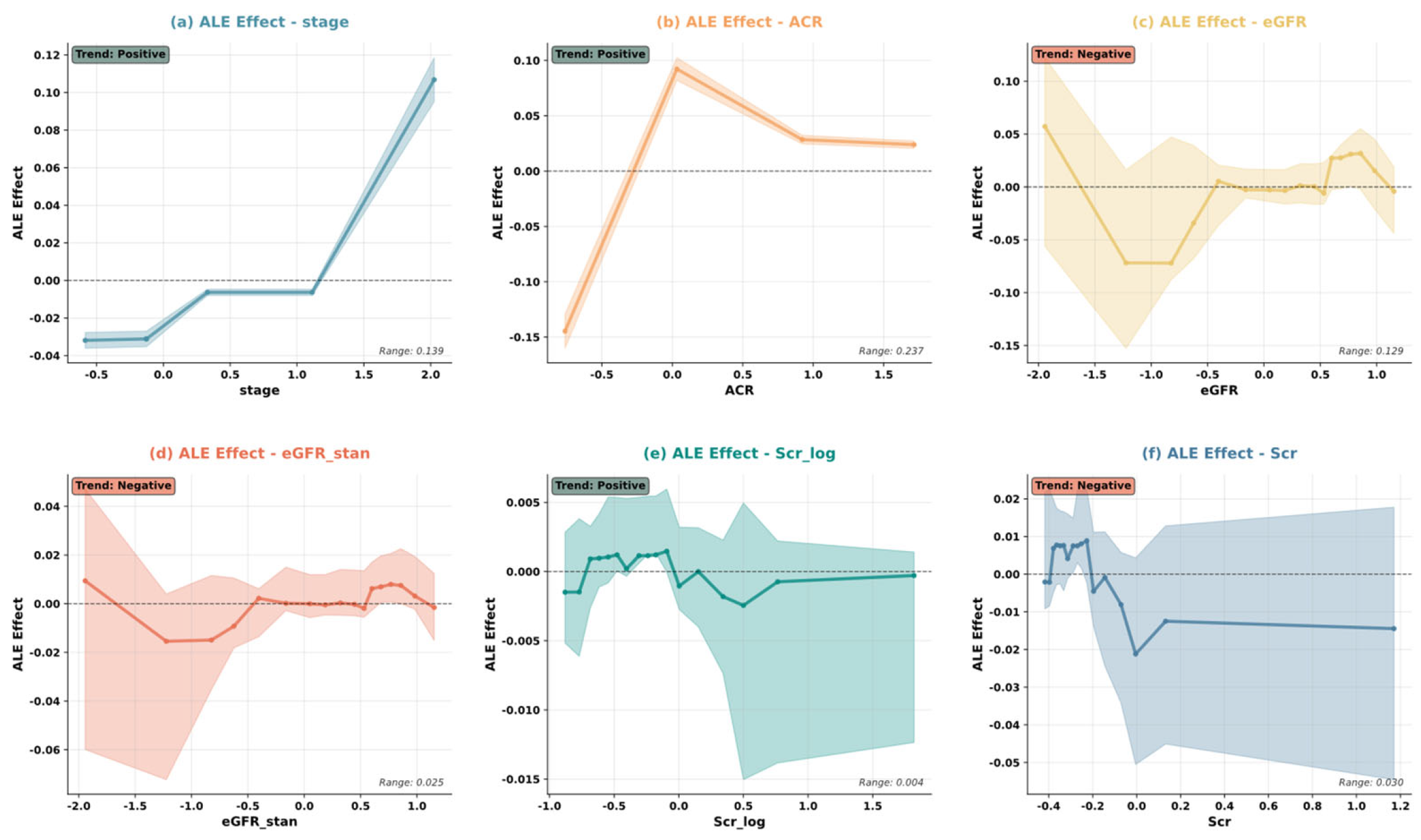
Figure 20 shows ALE plots quantifying marginal feature effects on CKD risk predictions while accounting for feature correlations, with 90% confidence intervals derived from bootstrap resampling. Panel (a) stage demonstrates a monotonic positive trajectory (effect range: 0.139) reflecting escalating risk contributions as disease severity advances. Panel (b) ACR exhibits the strongest effect magnitude (range: 0.237) with pronounced positive inflection beyond pathological thresholds, consistent with albuminuria-driven progression. Panel (c) eGFR reveals inverse correlation (range: 0.129) where declining renal filtration corresponds to elevated risk attribution, displaying characteristic nonlinear kinetics at critical functional thresholds. Panel (d) eGFR_stan shows attenuated but parallel protective effects (range: 0.025) following standardization. Panel (e) Scr_log presents minimal but consistent positive association (range: 0.004) with logarithmic transformation dampening extreme value influence. Panel (f) Scr manifests negative marginal effects (range: 0.030) with progressive attenuation, capturing the complex interplay between raw biomarker concentrations and model-predicted outcomes in the presence of covariate interactions.

5.5. Model Optimization and Algorithm Performance Analysis

Figure 21 demonstrates iterative feature selection workflow via Boruta algorithm, showcasing systematic elimination of redundant predictors while preserving discriminatory power. Panel (a) illustrates final feature partitioning with 11 confirmed variables (green, importance scores 0.4–1.0) achieving selection consensus, 0 tentative candidates remaining unresolved, and 13 rejected features (orange/red) identified as shadow-level contributors. Panel (b) traces the algorithmic convergence trajectory across 35 iterations, initiating with 24 original features, peaking at 48 features (incorporating shadow attributes), culminating in 36 candidates pre-finalization, and converging to 11 definitive predictors—representing a 54.2% dimensionality reduction without information loss. Panel (c) presents the intercorrelation structure among retained features (mean Pearson r = 0.349), revealing moderate associations between metabolic markers (Scr, eGFR cluster) and urinary indices (URC_HP, UP_index dyad) while maintaining sufficient independence to justify retention. Panel (d) quantifies the compactness gain, contrasting the original 24-dimensional feature space against the optimized 11-feature subset, achieving 54.2% reduction rate while preserving classification efficacy—validating Boruta’s capacity to identify the minimal sufficient feature set for robust CKD risk stratification.
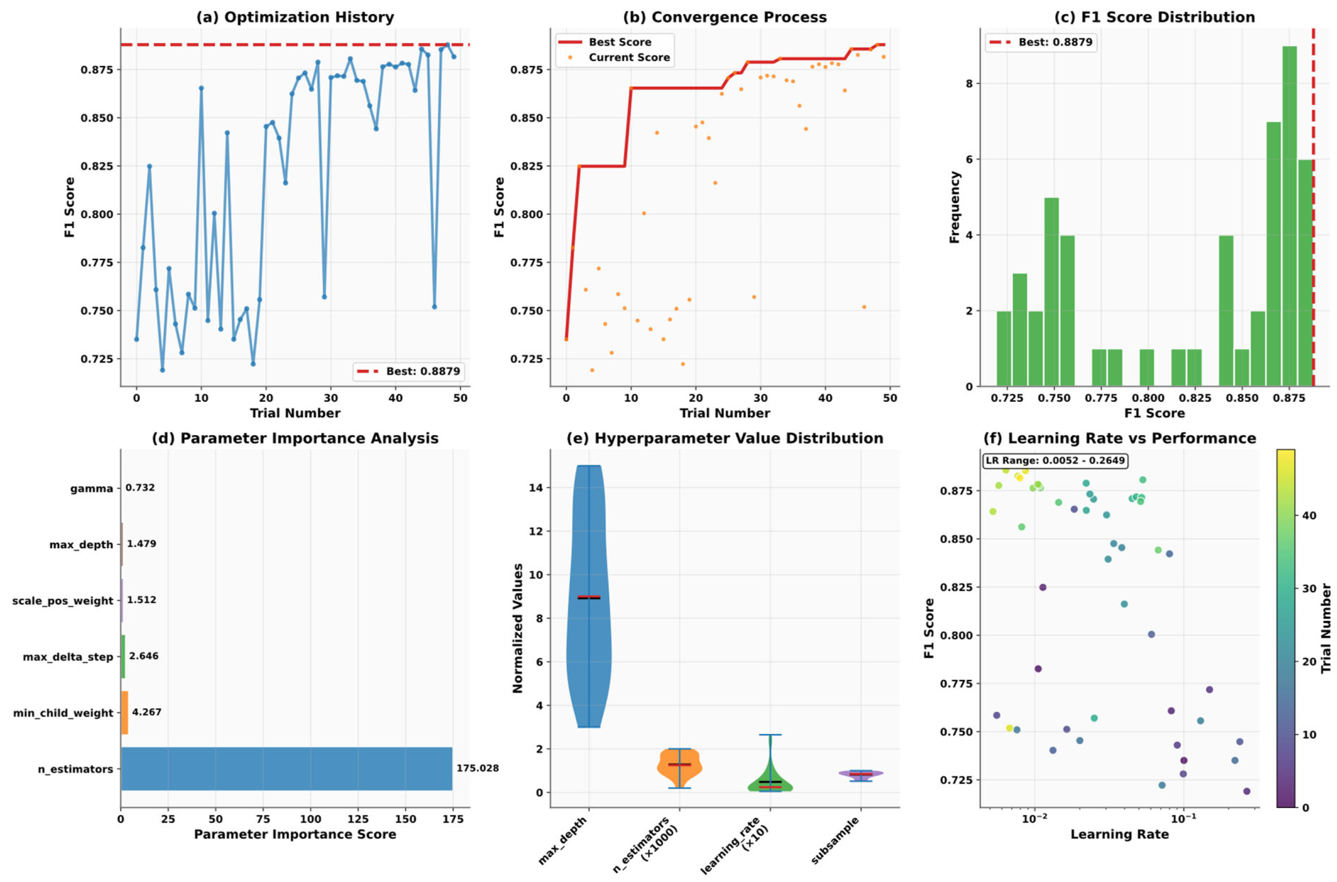
Figure 22 demonstrates comprehensive visualization of TPE-based hyperparameter search across 50 trials for CKD risk classifier optimization. Panel (a) optimization history exhibits stochastic exploration with peak F1-score of 0.879 achieved at trial convergence, demonstrating effective parameter space navigation. Panel (b) convergence dynamics reveal rapid initial improvement (trials 1–10) followed by exploitation-dominated refinement, with current scores (orange scatter) clustering near optimal threshold (red plateau). Panel (c) performance distribution shows bimodal density with primary mode at 0.875, indicating algorithmic convergence to superior parameter configurations. Panel (d) quantifies relative parameter influence via importance scores: n_estimators dominates (175.028), followed by gamma (0.722) and max_depth (1.479), establishing ensemble size as primary performance determinant. Panel (e) violin plots characterize hyperparameter sampling distributions—max_depth concentrates around 8–10, n_estimators spans 0.2–1.6 k trees (normalized), learning_rate exhibits narrow optimal band (0.005–0.25), and subsample remains uniformly explored. Panel (f) learning_rate-performance landscape reveals logarithmic sensitivity pattern with optimal zone (10−2 to 10−1), trial progression (colormap) demonstrating systematic exploration toward high-performing regions—validating adaptive sampling efficacy.
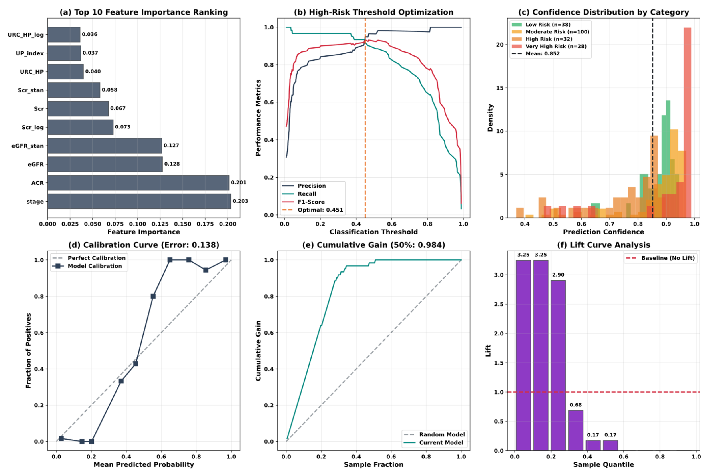
Figure 23 demonstrates diagnostic performance evaluation integrating feature attribution, decision threshold optimization, and predictive reliability metrics. Panel (a) XGBoost-derived feature importance hierarchy positions stage (0.203) and ACR (0.201) as co-primary determinants, with eGFR_stan (0.127) and eGFR (0.126) providing orthogonal renal function intelligence—validating the clinical primacy of disease staging and albuminuria in CKD prognostication. Panel (b) precision-recall-F1 trade-off surface identifies the optimal high-risk classification threshold at 0.451, balancing sensitivity (recall) and positive predictive value (precision) for actionable clinical decision-making in resource-constrained triage scenarios. Panel (c) stratified confidence distributions expose model certainty patterns: high-risk predictions (n = 28) concentrate at peak confidence (0.9–1.0), moderate/low-risk classes exhibit broader dispersion, with global mean at 0.892—quantifying epistemic uncertainty across risk strata. Panel (d) calibration analysis demonstrates near-perfect probabilistic alignment (mean absolute error: 0.138), with model predictions closely tracking ideal diagonal, confirming reliable probability estimates essential for trust-critical medical applications. Panel (e) cumulative gain curve achieves 98.4% positive case capture at 50% population screening, substantially outperforming random selection baseline—demonstrating twofold efficiency gain for targeted intervention programs. Panel (f) decile-stratified lift analysis reveals 3.23-fold enrichment in top decile declining to baseline parity, establishing prioritization framework for risk-stratified preventive care deployment—operationalizing model outputs into clinically actionable patient triaging protocols.
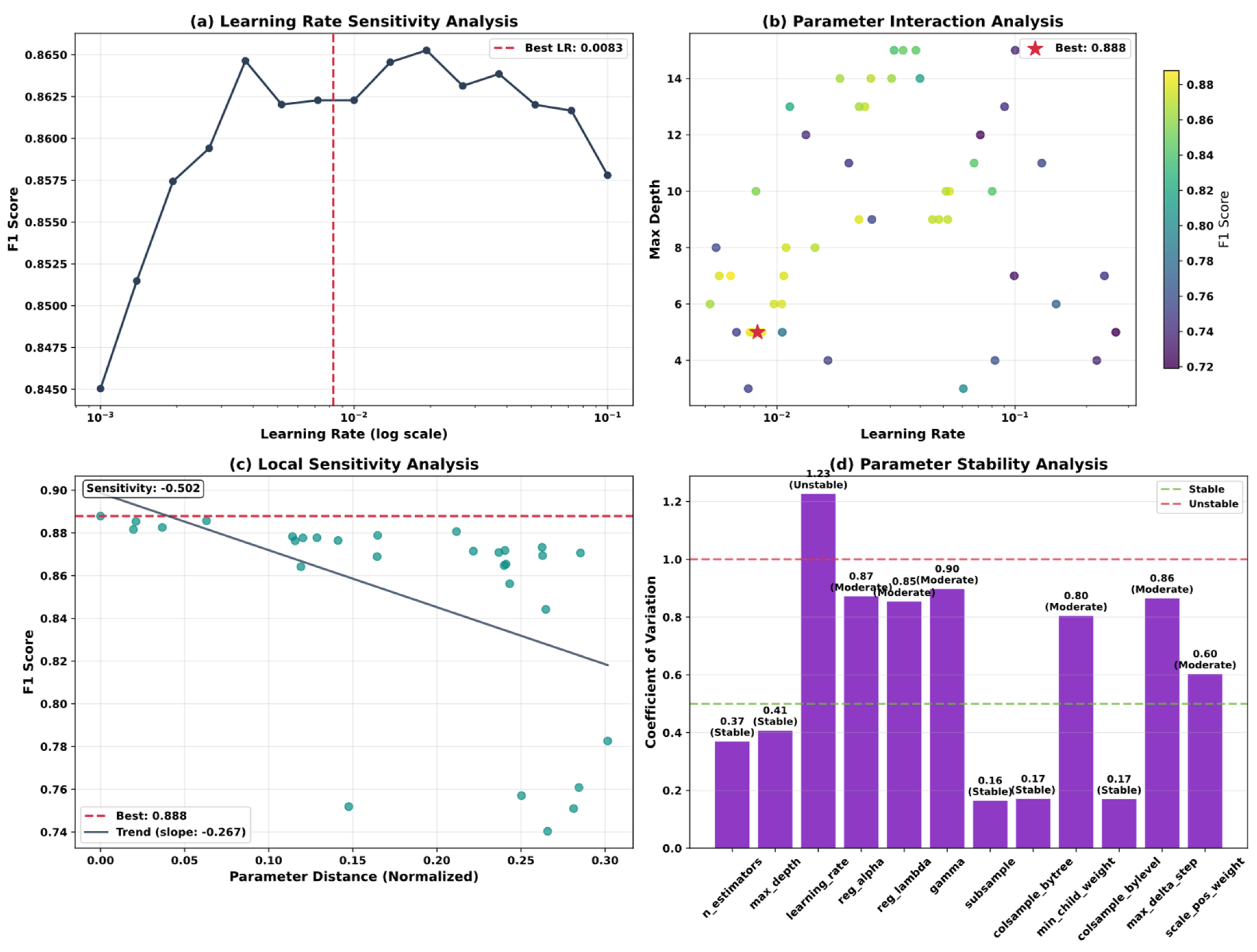
Figure 24 demonstrates perturbation analysis quantifying model robustness to hyperparameter variations and identifying critical optimization dependencies. Panel (a) learning rate sensitivity trajectory exhibits logarithmic performance dependence with the optimal region centered at 0.0083, demonstrating characteristic inverted-U pattern—initial steep ascent through underfitting regime (10−3 to 10−2·5), plateau maintenance across stable zone (10−2·5 to 10−2), followed by performance degradation beyond 10−1·5 indicating convergence instability. Panel (b) two-dimensional interaction landscape reveals learning rate-max depth synergy, with optimal configuration (LR = 0.0083, depth = 5, F1 = 0.888) residing in intermediate complexity zone—high-depth shallow-LR combinations yield suboptimal convergence, while extreme LR values destabilize performance regardless of architectural depth, validating the necessity of coordinated hyperparameter tuning. Panel (c) local sensitivity quantification around optimal solution shows moderate negative correlation (r = −0.502), with linear trend slope of −0.267 indicating gentle performance decay under parameter perturbation—robustness buffer is evident within 0.05 normalized distance, beyond which degradation accelerates, establishing practical tolerance margins for deployment parameter drift. Panel (d) stability profiling via coefficient of variation identifies learning_rate (CV = 1.23) as the most volatile exploration target contrasting with n_estimators (CV = 0.37) and max_depth (CV = 0.41), exhibiting stable convergence patterns, while reg_lambda (CV = 0.85) demonstrates moderate variability—the stability hierarchy informs adaptive sampling strategies where unstable parameters warrant denser exploration, while stable parameters permit coarser discretization for computational efficiency.
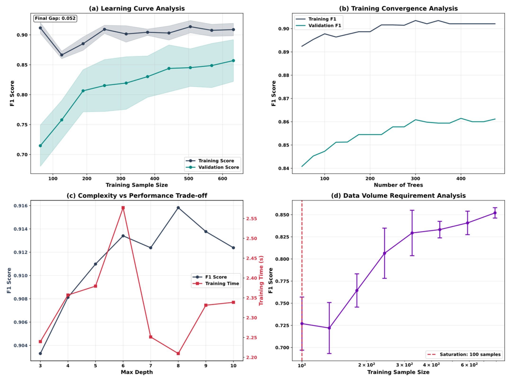
Figure 25 demonstrates evaluation of model learning behavior, convergence patterns, and data efficiency across architectural and sample size variations. Panel (a) learning curve analysis reveals rapid initial knowledge acquisition from minimal data (100 samples, F1 ≈ 0.72) ascending to performance plateau by 200 samples, with the training-validation gap converging to 0.052 at maximum dataset utilization—modest final divergence indicates well-calibrated model capacity without severe overfitting, while shaded confidence intervals demonstrate stable cross-validation reproducibility throughout sample size spectrum. Panel (b) ensemble convergence trajectory tracks F1 evolution across tree accumulation, exhibiting steep ascent through initial 100 estimators followed by asymptotic stabilization beyond 200 trees—the validation curve maintains a consistent 0.04–0.05 gap below training performance throughout, suggesting an optimal n_estimators range of 250–350, balancing predictive gain against diminishing marginal returns and computational overhead. Panel (c) architectural complexity trade-off quantifies the performance-efficiency Pareto frontier: F1 score peaks at depth 6 (0.916) before declining, while training time exhibits nonlinear escalation from 2.24 s (depth 3) to 2.56 s (depth 6)—the optimal sweet spot at depth 5–6 maximizes accuracy while constraining computational burden, beyond which overfitting penalties outweigh representational gains. Panel (d) data volume saturation analysis on logarithmic scale identifies critical inflection at 100 samples where performance stabilization initiates (F1 ≈ 0.73), with subsequent improvements yielding approximately 0.12 F1 gain through sixfold sample expansion to 600 samples—establishing a minimal viable dataset threshold for clinical deployment while quantifying an expected accuracy ceiling under data-limited scenarios, guiding prospective sample size planning for multi-center validation studies.
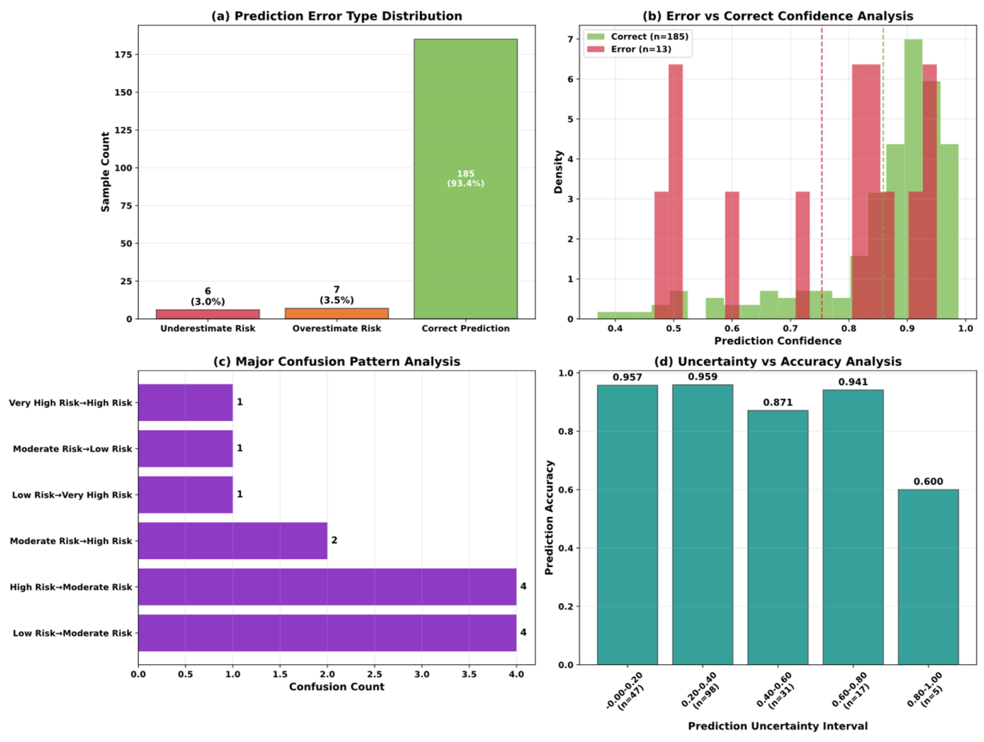
Figure 26 demonstrates misclassification characterization revealing error patterns, confidence distributions, and epistemic uncertainty correlates for model reliability assessment. Panel (a) error type stratification demonstrates exceptional overall accuracy (185/198 correct, 93.4%), with balanced directional bias: six underestimation errors (3.0%) versus seven overestimation errors (3.5%)—near-symmetric error distribution suggesting the absence of systematic prediction skew. Panel (b) confidence histogram dichotomy exposes predictive certainty disparity: correct classifications (n = 185) concentrate at high-confidence threshold (0.8–1.0 peak), contrasting sharply with error cases (n = 13) exhibiting bimodal distribution spanning 0.5–1.0 range—confidence gap serving as potential error detection signal, where predictions below 0.75 warrant enhanced clinical scrutiny. Panel (c) confusion pattern analysis identifies predominant misclassification trajectories: High Risk to Moderate Risk transitions dominate (n = 4), followed by Low-Moderate and Moderate-High bidirectional errors (n = 4 each)—notably absent are extreme cross-category errors, validating the model’s preservation of ordinal risk structure where misclassifications respect clinical severity adjacency. Panel (d) entropy-stratified accuracy reveals inverse uncertainty-performance relationship: maximum accuracy (0.957) achieved at minimal uncertainty (0.00–0.20 interval), declining to 0.600 at peak uncertainty (0.80–1.00)—establishing calibrated uncertainty estimates as reliable prediction quality indicators, enabling selective abstention protocols where high-entropy cases trigger automatic referral to specialist adjudication.

6. Conclusions

Chronic kidney disease affects over 850 million individuals worldwide, yet conventional machine learning approaches for risk stratification face critical obstacles: inefficient hyperparameter optimization, algorithmic opacity, and class imbalance. We developed and validated a comprehensive framework integrating Bayesian optimization with multi-method explainable artificial intelligence to address these challenges while ensuring clinical deployability.
Our approach delivered 93.43% accuracy, 93.13% F1-score, and 97.59% ROC-AUC through 5-fold cross-validation. Through 30 independent experiments, the model exhibited remarkable consistency (cross-validation standard deviation: 0.0121, generalization gap: −1.13%). The optimized framework achieved F1-score improvements of 6.22 percentage points beyond standard XGBoost and 7.0–26.8 percentage points compared to baseline algorithms, with all results derived from cross-validated estimates ensuring conservative performance expectations. Through 30 independent experiments, the model exhibited remarkable consistency (cross-validation standard deviation: 0.0121, generalization gap: −1.13%), with statistical analyses confirming superiority (p < 0.001, effect sizes d = 0.665–5.433). Tree-structured Parzen Estimator optimization necessitated merely 50 trials compared to 540 for exhaustive grid exploration, while Boruta-based feature selection accomplished 54.2% dimensionality reduction preserving predictive capacity. Four complementary interpretability techniques (SHAP, LIME, accumulated local effects, permutation importance) converged in identifying CKD stage and albumin-creatinine ratio as dominant prognostic factors, validating consistency with KDIGO clinical standards.
Practical clinical evaluation demonstrated 98.4% positive case identification at 50% population screening thresholds—achieving twofold efficiency gains for resource-constrained implementations. Probability calibration exhibited minimal deviation (mean absolute error: 0.138), supporting reliable risk quantification for therapeutic planning, while symmetric error patterns (3.0% underestimation, 3.5% overestimation) align with patient safety priorities. Decision curve evaluation confirmed sustained clinical value (peak net benefit: 0.28) across an actionable probability range of 0.0–0.85. Structural equation modeling revealed hyperuricemia (β = −3.19, p < 0.01) as the predominant modifiable risk determinant.
Several methodological constraints warrant acknowledgment. Our study is susceptible to single-dataset bias, as data originates from a single geographic region, albeit across seven institutions. This limits generalizability to populations with different genetic backgrounds, healthcare access patterns, and comorbidity profiles. Additional limitations include cross-sectional data precluding longitudinal trajectory modeling and moderate cohort size (n = 988). External validation using publicly available datasets (MIMIC, UCI) encountered feature incompatibility barriers; prospective multi-institutional validation necessitating 6–12 months for regulatory clearance and data aggregation is currently underway. Subsequent investigations should emphasize temporal progression modeling through longitudinal cohorts, pragmatic effectiveness trials in diverse clinical contexts, and privacy-preserving distributed learning frameworks enabling collaborative model refinement.
This investigation demonstrates that sophisticated interpretability frameworks can establish clinical guideline concordance while sustaining high discriminative performance, advancing trustworthy medical artificial intelligence. Integration of decision-analytic evaluation with confidence-stratified prediction protocols transforms computational capabilities into actionable clinical instruments, facilitating earlier risk-directed interventions preserving therapeutic windows.

Author Contributions

Methodology, J.H., D.Z., and M.H.; software, J.H. and D.Z.; validation, B.L., D.Z., and M.H.; data curation, J.H. and M.H.; writing—original draft preparation, J.H.; writing—reviewing and editing, B.L., D.Z., and M.H.; visualization, Z.L.; supervision, B.L.; funding acquisition, B.L. All authors have read and agreed to the published version of the manuscript.

Funding

This thesis was supported by the Key Research and Development Program of Guangxi Science and Technology Plan (Project No. 2023AB01361).

Data Availability Statement

Any further questions can be directed to the authors.

Conflicts of Interest

The authors declare no conflicts of interest.

References

  1. Ahmed, K.; Dubey, M.K.; Kajal; Dubey, S.; Pandey, D.K. Chronic Kidney Disease: Causes, Treatment, Management, and Future Scope. In Computational Intelligence for Genomics Data; Elsevier: Amsterdam, The Netherlands, 2025; pp. 99–111. ISBN 978-0-443-30080-6. [Google Scholar]
  2. Li, G.; Wan, Y.; Jiao, A.; Jiang, K.; Cui, G.; Tang, J.; Yu, S.; Hu, Z.; Zhao, S.; Yi, Z.; et al. Breaking Boundaries: Chronic Diseases and the Frontiers of Immune Microenvironments. Med Res. 2025, 1, 62–102. [Google Scholar] [CrossRef]
  3. Wu, J.; Yu, S.; Zhang, W.; Yang, Y.; Fang, S.; Pan, H.; Li, P.; Zhang, L. Guideline Concordance of Chronic Kidney Disease Testing Remains Low in Patients with Diabetes and Hypertension: Real-World Evidence from a City in Northwest China. Kidney Dis. 2025, 11, 610–620. [Google Scholar] [CrossRef]
  4. Alobaidi, S. Emerging Biomarkers and Advanced Diagnostics in Chronic Kidney Disease: Early Detection Through Multi-Omics and AI. Diagnostics 2025, 15, 1225. [Google Scholar] [CrossRef]
  5. Pradeep, U.; Chiwhane, A.; Acharya, S.; Daiya, V.; Kasat, P.R.; Sachani, P.; Mapari, S.A.; Bedi, G.N. A Comprehensive Review of Advanced Biomarkers for Chronic Kidney Disease in Older Adults: Current Insights and Future Directions. Cureus 2024, 16, e70413. [Google Scholar] [CrossRef]
  6. Dharmaraj, K.; Muthusamy, K.; Kannan, M.; Nanjan, M.; Ayyasamy, M.; Andrew, A.M. Diagnosing the Chronic Renal Disease Prediction by Using Random Forest and Bagged Tree. In Proceedings of the Second International Conference on Robotics, Automation and Intelligent Systems (ICRAINS 24), Coimbatore, India, 19 April 2025; p. 030010. [Google Scholar]
  7. Islam, R.; Sultana, A.; Islam, M.R. A Comprehensive Review for Chronic Disease Prediction Using Machine Learning Algorithms. J. Electr. Syst. Inf. Technol. 2024, 11, 27. [Google Scholar] [CrossRef]
  8. Anand, V.; Khajuria, A.; Pachauri, R.K.; Gupta, V. Optimized Machine Learning Based Comparative Analysis of Predictive Models for Classification of Kidney Tumors. Sci. Rep. 2025, 15, 30358. [Google Scholar] [CrossRef]
  9. Thota, K.K.; Gopala Krishna, J.S.V.; Sravani, K.; Panda, B.S.; Panda, G.; Shankar, R.S. A Model for Predicting Chronic Renal Failure Using CatBoost Classifier Algorithm and XGBClassifier. In Proceedings of the 2024 Second International Conference on Inventive Computing and Informatics (ICICI), Bangalore, India, 11–12 June 2024; IEEE: Piscataway, NJ, USA, 2024; pp. 96–102. [Google Scholar]
  10. Rahunathan, L.; Arun, G. Chronic Kidney Disease Prediction Using Light Gradient Boosting Machine. In Proceedings of the 2025 5th International Conference on Soft Computing for Security Applications (ICSCSA), Salem, India, 4–6 August 2025; IEEE: Piscataway, NJ, USA, 2025; pp. 1274–1280. [Google Scholar]
  11. Gogoi, P.; Valan, J.A. Machine Learning Approaches for Predicting and Diagnosing Chronic Kidney Disease: Current Trends, Challenges, Solutions, and Future Directions. Int. Urol. Nephrol. 2024, 57, 1245–1268. [Google Scholar] [CrossRef] [PubMed]
  12. Islam, R.; Sultana, A.; Tuhin, M.N. A Comparative Analysis of Machine Learning Algorithms with Tree-Structured Parzen Estimator for Liver Disease Prediction. Healthc. Anal. 2024, 6, 100358. [Google Scholar] [CrossRef]
  13. Ghosh, S.K.; Khandoker, A.H. Investigation on Explainable Machine Learning Models to Predict Chronic Kidney Diseases. Sci. Rep. 2024, 14, 3687. [Google Scholar] [CrossRef]
  14. Kaliappan, J.; Saravana Kumar, I.J.; Sundaravelan, S.; Anesh, T.; Rithik, R.R.; Singh, Y.; Vera-Garcia, D.V.; Himeur, Y.; Mansoor, W.; Atalla, S.; et al. Analyzing Classification and Feature Selection Strategies for Diabetes Prediction across Diverse Diabetes Datasets. Front. Artif. Intell. 2024, 7, 1421751. [Google Scholar] [CrossRef] [PubMed]
  15. Francis, A.; Harhay, M.N.; Ong, A.C.M.; Tummalapalli, S.L.; Ortiz, A.; Fogo, A.B.; Fliser, D.; Roy-Chaudhury, P.; Fontana, M.; Nangaku, M.; et al. Chronic Kidney Disease and the Global Public Health Agenda: An International Consensus. Nat. Rev. Nephrol. 2024, 20, 473–485. [Google Scholar] [CrossRef]
  16. Rahman, M.; Amin, A.; Hossain, J. Machine Learning Models for Chronic Kidney Disease Diagnosis and Prediction. Biomed. Signal Process. Control 2024, 87, 105368. [Google Scholar] [CrossRef]
  17. Yang, W.; Ahmed, N.; Barczak, A.L.C. Comparative Analysis of Machine Learning Algorithms for CKD Risk Prediction. IEEE Access 2024, 12, 171205–171220. [Google Scholar] [CrossRef]
  18. Metherall, B.; Berryman, A.K.; Brennan, G.S. Machine Learning for Classifying Chronic Kidney Disease and Predicting Creatinine Levels Using At-Home Measurements. Sci. Rep. 2025, 15, 4364. [Google Scholar] [CrossRef]
  19. Khan, N.; Raza, M.A.; Mirjat, N.H.; Balouch, N.; Abbas, G.; Yousef, A.; Touti, E. Unveiling the Predictive Power: A Comprehensive Study of Machine Learning Model for Anticipating Chronic Kidney Disease. Front. Artif. Intell. 2024, 6, 1339988. [Google Scholar] [CrossRef] [PubMed]
  20. Reddy, S.; Roy, S.; Choy, K.W.; Sharma, S.; Dwyer, K.M.; Manapragada, C.; Miller, Z.; Cheon, J.; Nakisa, B. Predicting Chronic Kidney Disease Progression Using Small Pathology Datasets and Explainable Machine Learning Models. Comput. Methods Programs Biomed. Update 2024, 6, 100160. [Google Scholar] [CrossRef]
  21. Sharifuzzaman, M.; Fahad, N.; Rabbi, R.I.; Sadib, R.J.; Haque Tusher, E.; Liew, T.H.; Naimul Islam, M.; Ullah Miah, M.S.; Hossen, M.J. Optimized Machine Learning Models and Stacking Hybrid Approach for Chronic Kidney Disease Prediction. In Artificial Intelligence Applications and Innovations; Maglogiannis, I., Iliadis, L., Andreou, A., Papaleonidas, A., Eds.; IFIP Advances in Information and Communication Technology; Springer Nature: Cham, Switzerland, 2025; Volume 758, pp. 196–212. ISBN 978-3-031-96234-9. [Google Scholar]
  22. Siregar, M.R.; Hartama, D.; Solikhun, S. Optimizing the KNN Algorithm for Classifying Chronic Kidney Disease Using Gridsearchcv. JITK 2025, 10, 680–689. [Google Scholar] [CrossRef]
  23. Singh, J.; Sandhu, J.K.; Kumar, Y. Metaheuristic-Based Hyperparameter Optimization for Multi-Disease Detection and Diagnosis in Machine Learning. SOCA 2024, 18, 163–182. [Google Scholar] [CrossRef]
  24. Kumar, A.; Singh, A.; Saxena, A.; Thakur, A.; Bhartiya, A.K. Enhanced Predictive Modeling for Chronic Kidney Disease Diagnosis. In Proceedings of the 2024 1st International Conference on Advanced Computing and Emerging Technologies (ACET), Ghaziabad, India, 23–24 August 2024; IEEE: Piscataway, NJ, USA, 2024; pp. 1–5. [Google Scholar]
  25. Luaha, L.; Fahmi, F.; Zarlis, M. Performance Analysis of Support Vector Machine (SVM) Model Through Parameter Optimization with Genetic Algorithm (GA) in Chronic Kidney Disease Classification. In Proceedings of the 2024 8th International Conference on Electrical, Telecommunication and Computer Engineering (ELTICOM), Medan, Indonesia, 21–22 November 2024; IEEE: Piscataway, NJ, USA, 2025; pp. 243–247. [Google Scholar]
  26. Jyothirmaye, S.; Meyyappan, S.; Ilavarasan, S.; Muthupandi, M.; Vallathan, G.; Kasturi, K.S. Revolutionizing CKD Prediction with Bayesian- Optimized LightGBM for Clinical Decision Support. In Proceedings of the 2025 International Conference on Emerging Technologies in Engineering Applications (ICETEA), Puducherry, India, 5–6 June 2025; IEEE: Piscataway, NJ, USA, 2025; pp. 1–6. [Google Scholar]
  27. Liu, Y.; Chen, J.; Wang, M. BO–FTT: A Deep Learning Model Based on Parameter Tuning for Early Disease Prediction from a Case of Anemia in CKD. Electronics 2025, 14, 2471. [Google Scholar] [CrossRef]
  28. Dharmarathne, G.; Bogahawaththa, M.; McAfee, M.; Rathnayake, U.; Meddage, D.P.P. On the Diagnosis of Chronic Kidney Disease Using a Machine Learning-Based Interface with Explainable Artificial Intelligence. Intell. Syst. Appl. 2024, 22, 200397. [Google Scholar] [CrossRef]
  29. Rezk, N.G.; Alshathri, S.; Sayed, A.; Hemdan, E.E.-D. Explainable AI for Chronic Kidney Disease Prediction in Medical IoT: Integrating GANs and Few-Shot Learning. Bioengineering 2025, 12, 356. [Google Scholar] [CrossRef]
  30. Manju, V.N.; Aparna, N.; Krishna Sowjanya, K. Decision Tree-Based Explainable AI for Diagnosis of Chronic Kidney Disease. In Proceedings of the 2023 5th International Conference on Inventive Research in Computing Applications (ICIRCA), Coimbatore, India, 3–5 August 2023; IEEE: Piscataway, NJ, USA, 2023; pp. 947–952. [Google Scholar]
  31. Tawsik Jawad, K.M.; Verma, A.; Amsaad, F.; Ashraf, L. A Study on the Application of Explainable AI on Ensemble Models for Predictive Analysis of Chronic Kidney Disease. IEEE Access 2025, 13, 23312–23330. [Google Scholar] [CrossRef]
  32. He, J.; Wang, X.; Zhu, P.; Wang, X.; Zhang, Y.; Zhao, J.; Sun, W.; Hu, K.; He, W.; Xie, J. Identification and Validation of an Explainable Early-Stage Chronic Kidney Disease Prediction Model: A Multicenter Retrospective Study. eClinicalMedicine 2025, 84, 103286. [Google Scholar] [CrossRef] [PubMed]
  33. Jiang, W.; Zhang, Y.; Weng, J.; Song, L.; Liu, S.; Li, X.; Xu, S.; Shi, K.; Li, L.; Zhang, C.; et al. Explainable Machine Learning Model for Predicting Persistent Sepsis-Associated Acute Kidney Injury: Development and Validation Study. J. Med. Internet Res. 2025, 27, e62932. [Google Scholar] [CrossRef] [PubMed]
  34. Chen, J.; Shen, C.; Xue, H.; Yuan, B.; Zheng, B.; Shen, L.; Fang, X. Development of an Early Prediction Model for Vomiting during Hemodialysis Using LASSO Regression and Boruta Feature Selection. Sci. Rep. 2025, 15, 10434. [Google Scholar] [CrossRef]
  35. Qin, J.; Dai, W.; Zhang, W.; Chen, B.; Liang, L.; Liang, C.; Lu, C.; Tan, Q.; Wei, C.; Tan, Y.; et al. Identification of Optimal Biomarkers Associated with Distant Metastasis in Breast Cancer Using Boruta and Lasso Machine Learning Algorithms. BMC Cancer 2025, 25, 1311. [Google Scholar] [CrossRef]
  36. Xu, C.; Shi, F.; Ding, W.; Fang, C.; Fang, C. Development and Validation of a Machine Learning Model for Cardiovascular Disease Risk Prediction in Type 2 Diabetes Patients. Sci. Rep. 2025, 15, 32818. [Google Scholar] [CrossRef] [PubMed]
  37. Sun, M.; Sun, X.; Wang, F.; Liu, L. Machine Learning-Based Prediction of Diabetic Peripheral Neuropathy: Model Development and Clinical Validation. Front. Endocrinol. 2025, 16, 1614657. [Google Scholar] [CrossRef]
  38. McShane, B.B.; Gal, D. Statistical Significance and the Dichotomization of Evidence. J. Am. Stat. Assoc. 2017, 112, 885–895. [Google Scholar] [CrossRef]
  39. Campagner, A.; Biganzoli, E.M.; Balsano, C.; Cereda, C.; Cabitza, F. Modeling Unknowns: A Vision for Uncertainty-Aware Machine Learning in Healthcare. Int. J. Med. Inform. 2025, 203, 106014. [Google Scholar] [CrossRef]
  40. Goligher, E.C.; Heath, A.; Harhay, M.O. Bayesian Statistics for Clinical Research. Lancet 2024, 404, 1067–1076. [Google Scholar] [CrossRef]
  41. Xia, T.; Dang, T.; Han, J.; Qendro, L.; Mascolo, C. Uncertainty-Aware Health Diagnostics via Class-Balanced Evidential Deep Learning. IEEE J. Biomed. Health Inform. 2024, 28, 6417–6428. [Google Scholar] [CrossRef]
  42. Koski, E.; Das, A.; Hsueh, P.-Y.S.; Solomonides, A.; Joseph, A.L.; Srivastava, G.; Johnson, C.E.; Kannry, J.; Oladimeji, B.; Price, A.; et al. Towards Responsible Artificial Intelligence in Healthcare—Getting Real about Real-World Data and Evidence. J. Am. Med. Inform. Assoc. 2025, 32, 1746–1755. [Google Scholar] [CrossRef] [PubMed]
  43. Huang, J.; Li, L.; Chen, J. Multi-Armed Bandit Optimization for Explainable AI Models in Chronic Kidney Disease Risk Evaluation. Symmetry 2025, 17, 1808. [Google Scholar] [CrossRef]
  44. Huang, J.; Li, L.; Hou, M.; Chen, J. Bayesian Optimization Meets Explainable AI: Enhanced Chronic Kidney Disease Risk Assessment. Mathematics 2025, 13, 2726. [Google Scholar] [CrossRef]
  45. Cornec-Le Gall, E.; Torres, V.E.; Harris, P.C. Genetic Complexity of Autosomal Dominant Polycystic Kidney and Liver Diseases. JASN 2018, 29, 13–23. [Google Scholar] [CrossRef]
  46. Zoccali, C.; Mallamaci, F.; Adamczak, M.; De Oliveira, R.B.; Massy, Z.A.; Sarafidis, P.; Agarwal, R.; Mark, P.B.; Kotanko, P.; Ferro, C.J.; et al. Cardiovascular Complications in Chronic Kidney Disease: A Review from the European Renal and Cardiovascular Medicine Working Group of the European Renal Association. Cardiovasc. Res. 2023, 119, 2017–2032. [Google Scholar] [CrossRef]
  47. Hallan, S.I.; Ritz, E.; Lydersen, S.; Romundstad, S.; Kvenild, K.; Orth, S.R. Combining GFR and Albuminuria to Classify CKD Improves Prediction of ESRD. J. Am. Soc. Nephrol. 2009, 20, 1069–1077. [Google Scholar] [CrossRef] [PubMed]
  48. Levey, A.S.; De Jong, P.E.; Coresh, J.; El Nahas, M.; Astor, B.C.; Matsushita, K.; Gansevoort, R.T.; Kasiske, B.L.; Eckardt, K.-U. The Definition, Classification, and Prognosis of Chronic Kidney Disease: A KDIGO Controversies Conference Report. Kidney Int. 2011, 80, 17–28. [Google Scholar] [CrossRef] [PubMed]
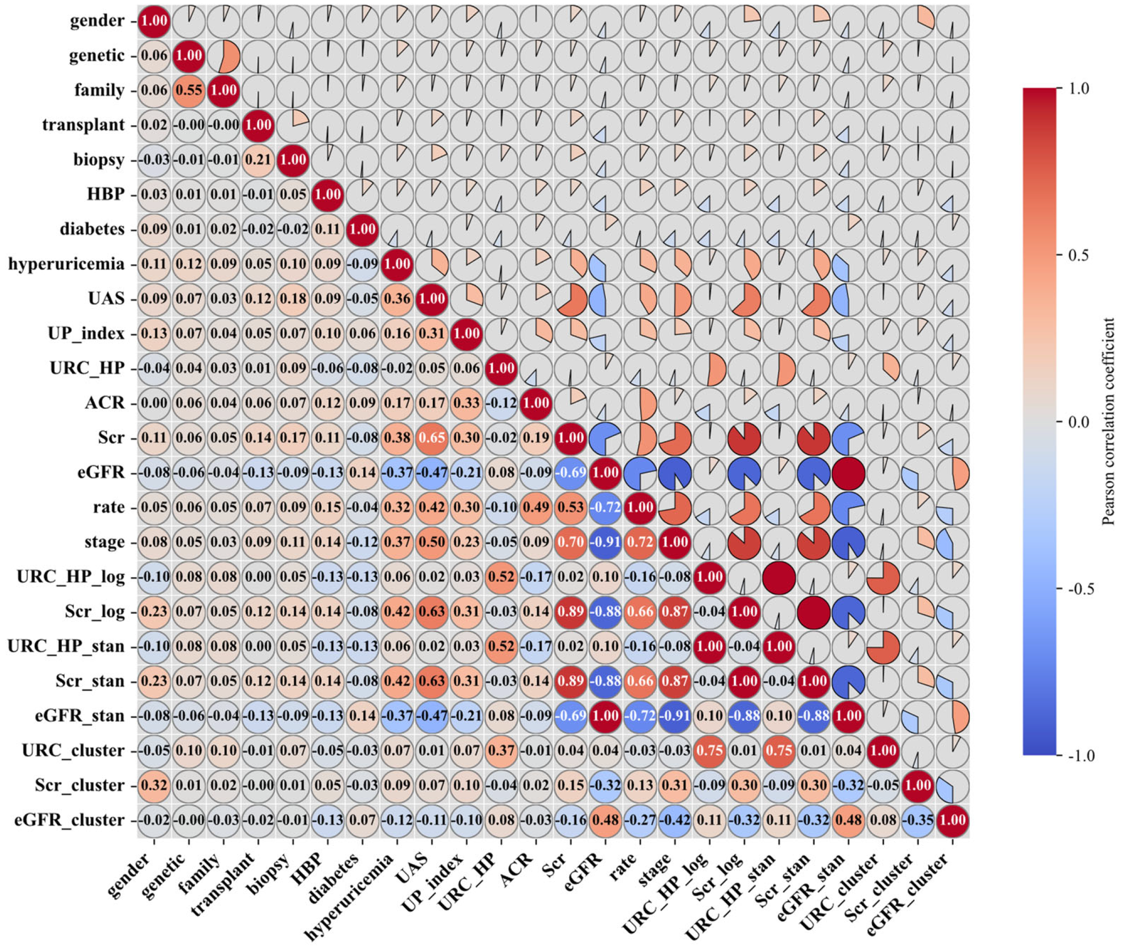
Figure 1. Pearson correlation analysis of renal function indicators and clinical features.
Symmetry 18 00081 g001
Figure 2. Clinical characteristics and risk distribution across CKD stages.
Symmetry 18 00081 g002
Figure 3. Biomarker relationships and multidimensional disease characterization.
Symmetry 18 00081 g003
Figure 4. Risk factor integration and disease progression pathways.
Symmetry 18 00081 g004
Figure 5. Dimensionality reduction and predictive disease modeling.
Symmetry 18 00081 g005
Figure 6. Structural equation model of CKD progression pathways.
Symmetry 18 00081 g006
Figure 7. Analytical workflow for CKD risk prediction.
Symmetry 18 00081 g007
Figure 8. Comparative Bayesian model evaluation framework.
Symmetry 18 00081 g008
Figure 9. Confusion matrix analysis of CKD risk classification methods.
Symmetry 18 00081 g009
Figure 10. ROC analysis for CKD Risk Levels.
Symmetry 18 00081 g010
Figure 11. Performance analysis of precision–recall curves.
Symmetry 18 00081 g011
Figure 12. Performance analysis of calibration curve.
Symmetry 18 00081 g012
Figure 13. Decision curve analysis.
Symmetry 18 00081 g013
Figure 14. Concordance index curves analysis.
Symmetry 18 00081 g014
Figure 15. SHAP value distributions across risk categories.
Symmetry 18 00081 g015
Figure 16. Individualized SHAP waterfall explanations by Risk Level.
Symmetry 18 00081 g016
Figure 17. Feature–target relationships revealed by SHAP dependence analysis.
Symmetry 18 00081 g017
Figure 18. Local feature contributions to risk classification via LIME analysis.
Symmetry 18 00081 g018
Figure 19. Model-agnostic feature importance via permutation testing.
Symmetry 18 00081 g019
Figure 20. Accumulated local effects profiling feature–outcome relationships.
Symmetry 18 00081 g020
Figure 21. Boruta-driven feature selection and dimensionality optimization.
Symmetry 18 00081 g021
Figure 22. Bayesian hyperparameter optimization trajectory analysis.
Symmetry 18 00081 g022
Figure 23. Multidimensional classification performance refinement.
Symmetry 18 00081 g023
Figure 24. Hyperparameter sensitivity landscape and stability profiling.
Symmetry 18 00081 g024
Figure 25. Training dynamics and scalability characterization.
Symmetry 18 00081 g025
Figure 26. Prediction error taxonomy and confidence-uncertainty profiling.
Symmetry 18 00081 g026
Table 1. Dataset field description.
Variable NameDescriptionValues/Range
hos_idHospital ID7 hospitals
hos_nameHospital NameHospital names
genderGenderMale/Female
geneticHereditary Kidney DiseaseY/N
familyFamily History of Chronic NephritisY/N
transplantKidney Transplant HistoryY/N
biopsyRenal Biopsy HistoryY/N
HBPHypertension HistoryY/N
diabetesDiabetes Mellitus HistoryY/N
hyperuricemiaHyperuricemiaY/N
UASUrinary Anatomical Structure Abnormality−/Y/N
ACRAlbumin-to-Creatinine Ratio<30/30–300/>300 mg/g
UP_positiveUrine Protein TestNegative/Positive
UP_indexUrine Protein Index± (0.1–0.2 g/L)
+ (0.2–1.0)
2+ (1.0–2.0)
3+ (2.0–4.0)
5+ (>4.0)
URC_unitUrine RBC UnitHP-per high power field
μL-per microliter
URC_numUrine RBC Count0–93.9
Different units
ScrSerum Creatinine0/27.2–85,800 μmol/L
eGFREstimated Glomerular Filtration Rate2.5–148 mL/min/1.73 m2
dateDiagnosis Date13 December 2016–27 January 2018
rateCKD Risk StratificationLow/Moderate/High/Very High Risk
stageCKD StageCKD Stage 1/2/3/4/5
Table 2. Model performance comparison results.
ModelAccuracyPrecisionRecallF1MCCCohen KappaROC AUCCV_MeanCV_Std
Ours0.93430.94110.92310.93130.90280.90200.97590.88350.0181
XGBoost0.87880.87540.86340.86910.820.81980.95680.84560.013
LightGBM0.87370.86610.85780.86140.81320.81310.95820.84050.0141
CatBoost0.86870.86290.83070.84520.80390.80240.9630.85440.0165
Voting0.86360.87230.82970.84870.79620.79420.96340.82910.0144
RandomForest0.86360.86440.8360.84910.79650.79540.96390.82780.0189
Bagging0.85860.86140.82840.84330.78870.78720.96510.83040.0152
Stacking0.85860.85860.82350.83850.78880.78670.95960.83040.0298
GBDT0.85350.85380.82580.83880.78130.78020.95790.81650.0139
KNeighbors0.85350.85580.810.82930.78090.77830.92090.82280.004
ExtraTrees0.85350.8640.80440.82710.78180.7760.96280.80630.0203
AdaBoost0.84340.84910.79580.81680.7660.76110.93470.81390.0221
SVM0.83840.83720.78390.80550.7580.75330.95260.82780.0162
Logistic0.83330.83940.79550.81330.75040.74730.94980.80630.013
ElasticNet0.83330.83940.79550.81330.75040.74730.95010.80510.0167
Lasso0.82830.83160.79290.80910.74280.74030.94990.80630.0153
DecisionTree0.81310.80790.74530.76940.71890.71370.89990.74430.0242
MLP0.79290.79510.72470.73350.69260.67750.93550.72910.0493
GaussianNB0.74750.77050.71910.7310.63330.62830.9080.69870.0403
Ridge0.72730.69760.64030.62210.59130.56930.89990.70130.0221
Perceptron0.65150.66670.71530.66640.54930.5270.89990.67090.0243
Table 3. Bayesian-Frequentist dual validation: Performance metrics (n = 30).
ModelAccuracyPrecisionRecallF1MCCCohen KappaROC AUC
Ours0.860 ± 0.0230.859 ± 0.0270.844 ± 0.0250.850 ± 0.0250.793 ± 0.0340.792 ± 0.0340.946 ± 0.014
Stacking0.850 ± 0.0270.846 ± 0.0290.821 ± 0.0320.831 ± 0.0300.776 ± 0.0410.775 ± 0.0410.948 ± 0.014
Lasso0.844 ± 0.0220.854 ± 0.0260.813 ± 0.0250.828 ± 0.0240.768 ± 0.0340.764 ± 0.0340.943 ± 0.012
ElasticNet0.840 ± 0.0200.850 ± 0.0260.809 ± 0.0210.824 ± 0.0220.762 ± 0.0300.758 ± 0.0300.941 ± 0.012
Logistic0.834 ± 0.0200.838 ± 0.0260.802 ± 0.0220.816 ± 0.0230.753 ± 0.0300.750 ± 0.0300.937 ± 0.013
Voting0.835 ± 0.0260.839 ± 0.0320.798 ± 0.0300.815 ± 0.0300.754 ± 0.0380.750 ± 0.0380.947 ± 0.012
AdaBoost0.829 ± 0.0310.831 ± 0.0350.798 ± 0.0360.811 ± 0.0350.746 ± 0.0460.744 ± 0.0460.937 ± 0.013
XGBoost0.823 ± 0.0270.815 ± 0.0400.782 ± 0.0340.794 ± 0.0360.736 ± 0.0410.734 ± 0.0410.945 ± 0.013
LightGBM0.827 ± 0.0270.838 ± 0.0420.772 ± 0.0360.793 ± 0.0380.742 ± 0.0420.734 ± 0.0420.948 ± 0.013
Bagging0.816 ± 0.0230.825 ± 0.0360.756 ± 0.0310.774 ± 0.0330.726 ± 0.0360.717 ± 0.0370.945 ± 0.014
SVM0.788 ± 0.0220.789 ± 0.0310.723 ± 0.0310.746 ± 0.0290.681 ± 0.0350.673 ± 0.0340.941 ± 0.015
CatBoost0.801 ± 0.0180.814 ± 0.0380.728 ± 0.0230.741 ± 0.0270.705 ± 0.0290.688 ± 0.0290.932 ± 0.013
GBDT0.778 ± 0.0250.795 ± 0.0410.702 ± 0.0300.726 ± 0.0310.668 ± 0.0400.651 ± 0.0400.940 ± 0.014
RandomForest0.758 ± 0.0330.784 ± 0.0420.687 ± 0.0370.716 ± 0.0380.637 ± 0.0530.620 ± 0.0530.929 ± 0.014
KNeighbors0.723 ± 0.0320.735 ± 0.0370.660 ± 0.0380.686 ± 0.0360.579 ± 0.0500.571 ± 0.0500.877 ± 0.019
Perceptron0.705 ± 0.0480.694 ± 0.0500.686 ± 0.0450.681 ± 0.0430.569 ± 0.0630.563 ± 0.0630.000 ± 0.000
DecisionTree0.694 ± 0.0370.710 ± 0.0460.642 ± 0.0420.661 ± 0.0420.540 ± 0.0560.532 ± 0.0560.854 ± 0.023
MLP0.707 ± 0.0470.684 ± 0.0700.642 ± 0.0550.645 ± 0.0640.557 ± 0.0740.546 ± 0.0760.877 ± 0.034
ExtraTrees0.715 ± 0.0190.814 ± 0.0640.608 ± 0.0250.624 ± 0.0290.581 ± 0.0330.528 ± 0.0340.923 ± 0.014
Ridge0.713 ± 0.0230.705 ± 0.0810.632 ± 0.0220.613 ± 0.0230.569 ± 0.0380.548 ± 0.0360.000 ± 0.000
GaussianNB0.431 ± 0.1190.489 ± 0.1130.542 ± 0.0650.450 ± 0.0970.352 ± 0.0940.276 ± 0.1190.857 ± 0.022
Table 4. Cross-validation stability with dual statistical inference.
ModelCV_F1CV_MeanCV_StdCV_Rangep-Value95% CIEffect Size95%
Credible
Interval
Generalization
Gap
Ours0.849 ± 0.0120.84910.0121[0.8231, 0.8713]−0.0113
Stacking0.816 ± 0.0110.81630.0108[0.7953, 0.8379]<0.001[0.010, 0.027]0.665[0.011, 0.026]−0.0333
Lasso0.823 ± 0.0080.82320.0085[0.8074, 0.8401]<0.001[0.013, 0.031]0.873[0.013, 0.031]−0.0210
ElasticNet0.819 ± 0.0100.81880.0095[0.8036, 0.8424]<0.001[0.015, 0.036]1.067[0.015, 0.035]−0.0214
Logistic0.810 ± 0.0080.80950.0085[0.7936, 0.8286]<0.001[0.024, 0.044]1.412[0.024, 0.044]−0.0247
Voting0.800 ± 0.0110.80020.0107[0.7734, 0.8274]<0.001[0.027, 0.044]1.278[0.027, 0.043]−0.0348
AdaBoost0.807 ± 0.0130.80680.0134[0.7679, 0.8287]<0.001[0.029, 0.048]1.267[0.029, 0.048]−0.0227
XGBoost0.760 ± 0.0150.75960.0147[0.7276, 0.7900]<0.001[0.045, 0.066]1.795[0.045, 0.065]−0.0638
LightGBM0.783 ± 0.0170.78320.0172[0.7517, 0.8190]<0.001[0.046, 0.068]1.749[0.046, 0.067]−0.0436
Bagging0.765 ± 0.0200.76460.0195[0.7225, 0.7948]<0.001[0.065, 0.086]2.566[0.065, 0.085]−0.0517
SVM0.705 ± 0.0200.70530.0197[0.6678, 0.7427]<0.001[0.093, 0.115]3.799[0.093, 0.114]−0.0828
CatBoost0.731 ± 0.0160.73100.0160[0.7039, 0.7642]<0.001[0.099, 0.119]4.139[0.099, 0.118]−0.0695
GBDT0.677 ± 0.0130.67670.0128[0.6538, 0.7051]<0.001[0.114, 0.134]4.4[0.114, 0.133]−0.1013
RandomForest0.715 ± 0.0210.71480.0208[0.6718, 0.7482]<0.001[0.121, 0.146]4.166[0.121, 0.145]−0.0436
KNeighbors0.679 ± 0.0140.67870.0135[0.6548, 0.7062]<0.001[0.150, 0.177]5.259[0.150, 0.175]−0.0442
Perceptron0.674 ± 0.0190.67420.0189[0.6366, 0.7221]<0.001[0.151, 0.187]4.795[0.150, 0.185]−0.0304
DecisionTree0.650 ± 0.0230.65000.0234[0.6152, 0.7166]<0.001[0.171, 0.207]5.433[0.170, 0.205]−0.0438
MLP0.609 ± 0.0490.60940.0487[0.4918, 0.6686]<0.001[0.178, 0.232]4.243[0.177, 0.227]−0.0976
ExtraTrees0.615 ± 0.0170.61500.0170[0.5859, 0.6442]<0.001[0.214, 0.238]8.361[0.214, 0.237]−0.0997
Ridge0.619 ± 0.0110.61850.0113[0.5970, 0.6388]<0.001[0.226, 0.247]9.707[0.225, 0.246]−0.0943
GaussianNB0.444 ± 0.0510.44370.0509[0.3621, 0.5626]<0.001[0.364, 0.435]5.653[0.354, 0.420]0.0131
Table 5. Hyperparameter search space specifications across optimization approaches.
ModelN_EstimatorsMax_DepthLearning_RateSubsampleColsample_Bytree
Ours(200, 2000)(3, 15)log(0.005–0.3)(0.5, 1.0)(0.5, 1.0)
ASHA(100, 2000)(3, 15)(0.01, 0.3)(0.5, 1.0)(0.5, 1.0)
Auto-sklearn[50, 2000][3, 15][0.01, 0.3][0.5, 1.0][0.5, 1.0]
BOHB(200, 2000)(3, 15)(0.01, 0.3)(0.5, 1.0)(0.5, 1.0)
CMA-ES(100, 2000)(3, 15)(0.01, 0.3)(0.5, 1.0)(0.5, 1.0)
Differential Evolution(100, 2000)(3, 15)(0.01, 0.3)(0.5, 1.0)(0.5, 1.0)
FLAML[50, 2000][3, 15][0.01, 0.3][0.6, 1.0][0.6, 1.0]
Genetic Algorithm(100, 2000)(3, 15)(0.01, 0.3)(0.5, 1.0)(0.5, 1.0)
Grid Search[100, 800][3, 8][0.01, 0.2][0.7, 1.0][0.7, 1.0]
H2O AutoML[50, 2000][4, 15][0.03, 0.3][0.7, 1.0][0.7, 1.0]
Hyperband[100, 2000][3, 15](0.01, 0.3)(0.5, 1.0)(0.5, 1.0)
Hyperopt[100, 2000][3, 15](0.01, 0.3)(0.5, 1.0)(0.5, 1.0)
MAB[200, 2000][3, 15][0.05–0.3][0.8, 1.0][0.8, 1.0]
PSO(100, 2000)(3, 15)(0.01, 0.3)(0.5, 1.0)(0.5, 1.0)
PBT(100, 2000)(3, 15)log(0.01–0.3)(0.5, 1.0)(0.5, 1.0)
Random Search[200, 2000][3, 15][0.005, 0.3][0.5, 1.0][0.5, 1.0]
Scikit-Optimize(100, 2000)(3, 15)(0.01, 0.3)(0.5, 1.0)(0.5, 1.0)
Successive Halving(100, 2000)(3, 15)log(0.01–0.3)(0.5, 1.0)(0.5, 1.0)
Thompson Sampling[200, 2000][3, 15][0.05, 0.3][0.8, 1.0][0.8, 1.0]
UCB[100, 2000][3, 15][0.01, 0.3][0.5, 1.0][0.5, 1.0]
Table 6. Hyperparameter configuration comparison across optimization methods.
ModelAccuracyPrecisionRecallF1MCCCohen
Kappa
ROC
AUC
CV
Mean
CV
Std
Generalization
Gap
Evaluations
Ours0.93430.94110.92310.93130.90280.90200.97590.88350.0182−0.050850
Random
Search
0.92930.93200.91550.92270.89530.89450.97690.86840.0129−0.060950
PBT0.92420.92470.91290.91800.88780.88720.97070.86330.0065−0.061050
Scikit-
Optimize
0.92420.92700.90530.91500.88770.88690.96840.88480.0185−0.039450
UCB0.91920.92030.90040.90840.88050.87920.97530.86840.0152−0.050850
FLAML0.91410.90830.89640.90150.87280.87220.96860.88100.0194−0.03311069
Grid
Search
0.91410.91060.89500.90200.87270.87210.97010.88350.0206−0.0306540
Hyperopt0.91410.91060.89500.90200.87270.87210.97090.87970.0144−0.034450
Successive
Halving
0.91410.91030.90760.90830.87310.87280.96880.86200.0074−0.052172
H2O
AutoML
0.90910.90520.89040.89630.86540.86440.97140.96080.00620.051716
Genetic
Algorithm
0.90910.90510.89510.89840.86560.86470.96700.86200.0157−0.047156
PSO0.90910.90450.89240.89760.86540.86490.96970.87970.0212−0.029360
ASHA0.89900.89520.88490.88820.85050.84960.96700.86080.0170−0.038250
Hyperband0.89900.89030.88360.88600.85050.85000.96790.87720.0095−0.021850
Differential
Evolution
0.89900.89690.87730.88630.85000.84920.97800.87720.0218−0.021860
Auto-sklearn0.89390.88400.88590.88390.84400.84360.96210.91650.03030.0225283
BOHB0.88890.87990.87340.87580.83540.83500.96460.85820.0182−0.030750
CMA-ES0.88890.87990.87340.87580.83540.83500.96620.86580.0217−0.023150
MAB0.88380.87340.87070.87140.82810.82790.96490.86960.0239−0.014250
Thompson
Sampling
0.88380.87340.87070.87140.82810.82790.96490.86960.0239−0.014250
Disclaimer/Publisher’s Note: The statements, opinions and data contained in all publications are solely those of the individual author(s) and contributor(s) and not of MDPI and/or the editor(s). MDPI and/or the editor(s) disclaim responsibility for any injury to people or property resulting from any ideas, methods, instructions or products referred to in the content.