Nonlocal Effective Field Theory and Its Applications

Abstract

We review recent applications of nonlocal effective field theory, particularly focusing on nonlocal chiral effective theory and nonlocal quantum electrodynamics (QED), as well as an extension of nonlocal effective theory to curved spacetime. For the chiral effective theory, we discuss the calculation of generalized parton distributions (GPDs) of the nucleon at nonzero skewness, along with the corresponding gravitational (or mechanical) form factors, within the convolution framework. In the QED application, we extend the nonlocal formulation to construct the most general nonlocal QED interaction, in which both the propagator and fundamental QED vertex are modified due to the nonlocal Lagrangian, while preserving the Ward–Green–Takahashi identities. For consistency with the modified propagator, a solid quantization is proposed, and the nonlocal QED is applied to explain the lepton $g-2$ anomalies without the introduction of new particles beyond the standard model. Finally, with an extension of the chiral effective action to curved spacetime, we investigate the nonlocal energy–momentum tensor and gravitational form factors of the nucleon with a nonlocal pion–nucleon interaction.

1. Introduction

Since the discovery of the finite size of the proton in the 1950s, extensive theoretical and experimental work has greatly expanded our knowledge of the inner structure of the nucleon. Examples that have challenged our understanding include the proton spin puzzle [1,2,3,4,5,6,7,8,9,10,11,12,13,14,15,16,17,18,19], the flavor asymmetry in the proton sea [20,21,22,23,24,25,26,27,28,29,30,31,32,33,34,35,36,37,38], and, more recently, the proton electric radius puzzle [39,40,41,42,43,44,45,46,47,48]. With the increased energies and luminosities available at new facilities and upgrading of experimental equipment, considerable progress has been made in recent years in extracting quantitative information about nucleon structure, characterized in the form of nucleon form factors, parton distribution functions (PDFs), and generalized parton distributions (GPDs).

GPDs, in particular, contain rich information about the 3-dimensional structure of hadrons, in terms of their fundamental quark and gluon constituents. These describe the distributions of partons carrying a specific fraction x of the hadron’s light-front momentum, squared four-momentum transfer t, and skewness $\xi$. Information about GPDs of the nucleon, or more specifically about their Compton form factors, can be obtained through processes such as deeply-virtual Compton scattering (DVCS), deeply virtual meson production (DVMP), and time-like Compton scattering (TCS). More recently, a new set of processes, referred to as single diffractive hard exclusive photoproduction (SDHEP), has been proposed as a way of accessing the x dependence of the GPDs directly from the experiment [49,50].

The determination of GPDs has become one of the important scientific goals at accelerator facilities around the world. Many measurements of observables sensitive to nucleon GPDs or their moments have been performed over a wide range of kinematics through unpolarized and polarized experiments at DESY (HERMES, H1, and ZEUS experiments) and Jefferson Lab (CLAS) [51,52,53,54,55,56,57,58,59,60,61,62]. Future experiments are planned for Jefferson Lab’s Halls A, B and C, at J-PARC in Japan, COMPASS at CERN, and the planned Electron-Ion Collider (EIC) and Large Hadron–electron Collider (LHeC) [63,64,65,66,67,68,69,70,71,72].

The GPDs are closely related to the electromagnetic elastic and transition form factors. Integrating over the momentum fraction x, one obtains the Mellin moments of the GPDs, or generalized form factors (GFFs). For the lowest-order form factors, there has been considerable theoretical and experimental study over the past few decades. Higher-order generalized form factors, such as the gravitational (or mechanical) form factors, have attracted growing interest recently [73]. The gravitational form factors are related to the matrix elements of the energy–momentum tensor, reflecting the bulk properties of hadrons, such as mass, spin, and pressure, and can be extracted from DVCS and exclusive meson production [74,75]. Rather than integrating over the GPDs, the gravitational form factors can also be obtained directly from lattice QCD or chiral effective theory calculations [76,77,78,79]. The GPDs provide information about the distribution of partons inside the nucleon, while the GFFs reflect information about the overall properties of the nucleon. These two types of functions provide us with important insights into the structure of the nucleon from different perspectives.

On the theory side, lattice QCD is the most rigorous approach that is based directly on the fundamental QCD theory. Since PDFs are defined in Minkowski space, it has not been possible to simulate PDFs directly on a Euclidean lattice. In recent years, however, quasi-PDFs have been proposed as a means of indirectly accessing the light-front distributions from lattice simulations within the large-momentum effective theory (LaMET) approach [80]. Alternatively, pseudo-PDFs have also been suggested, involving ratios of equal-time matrix elements of the Wilson line between quarks to the rest-frame density matrix elements, and parametrized in terms of the Ioffe time [81,82,83,84,85,86]. A number of lattice groups have computed unpolarized PDFs [87,88,89], helicity-dependent PDFs [34,90,91], and transversity PDFs [90,92,93], using either the quasi-PDF or pseudo-PDF approach, although the efforts are generally still in their early stages. In addition, the higher-order GFFs, such as the gravitational form factors, have also been simulated on the lattice [76,77].

Another systematical approach used in hadronic physics applications has been chiral effective field theory (EFT), a specific example of which is chiral perturbation theory ($\chi$PT). This allows the description of low-energy properties and processes within a perturbative approach, emphasizing the chiral symmetry aspects of QCD. Historically, most formulations of $\chi$PT have utilized dimensional or infrared regularization [94,95,96,97] and the extended on-mass-shell renormalization scheme [98,99,100]. Although $\chi$PT has been a fairly successful approach, it can only describe physical quantities at rather low momentum transfers. For example, for the nucleon form factors, it is only valid at relatively small $Q^2$ values, $Q^2\lesssim 0.1$ GeV² [101]. The range can be extended up to $Q^2\lesssim 0.4$ GeV² by explicitly including vector meson degrees of freedom into the theory [96,102]. An alternative regularization method, finite-range regularization (FRR), has been argued to achieve better convergence than dimensional regularization in the calculation of many hadronic observables [103,104,105]. EFT with FRR has been applied in the investigation of the vector meson mass, nucleon magnetic moments, electric and magnetic radii, the $Q^2$ dependence of electromagnetic and weak form factors, and moments of PDFs and GPDs [106,107,108,109,110]. Earlier treatments with nonrelativistic regulators in the FRR EFT have also more recently been generalized to relativistic versions by making the regulators four-dimensional functions or using Pauli–Villars regularization [111,112].

In recent years, a nonlocal chiral effective theory has been proposed, which reflects the non-point-like properties of hadrons. In the nonlocal theory, the local meson–baryon interactions are replaced by nonlocal interactions, where the baryon field is defined at a spacetime point x and the meson or photon field is displaced by a distance a to spacetime point $x+a$ [113]. A correlation function, $F\left(a\right)$, parametrizes the nonlocal interaction. To guarantee local gauge invariance, a gauge link is introduced, generating additional Feynman diagrams that are essential for preserving charge conservation. The nonlocal chiral effective theory has been successfully applied to the calculation of nucleon form factors, strange form factors, unpolarized and polarized PDFs, and GPDs with zero and nonzero skewness [36,114,115,116,117,118,119,120,121,122].

Beyond chiral effective theory, in Refs. [123,124] a nonlocal formulation of QED was proposed and applied to the study of the lepton $g-2$ anomaly. The anomalous magnetic moments of the electron and muon, $a_e$ and $a_{\mu }$, are some of the most precisely determined quantities in particle physics [125]. Recent measurement of the muon anomalous magnetic moment in the E989 experiment at Fermilab showed a $3.3\sigma$ discrepancy from the standard model (SM) prediction [126]. Combined with the previous E821 result from BNL [127], the measurements revealed a $4.2\sigma$ deviation from the SM. For the electron, the most accurate measurement of $a_e$ was carried out by the Harvard group, and the discrepancy from the SM with the fine structure constant $\alpha$ measured at Berkeley was $2.4\sigma$ [128,129,130]. However, a new determination of $\alpha$ from the Laboratoire Kastler Brossel (LKB) improves the accuracy by a factor of 2.5 compared to the previous Berkeley measurement [131]. With this new $\alpha$, the SM prediction for the electron magnetic moment is $1.6\sigma$ below the experiment. Possible solutions to the discrepancy have been proposed, typically by introducing new particles, symmetries, and interactions beyond the SM [132,133,134,135,136,137,138,139,140,141,142,143,144,145,146,147,148,149,150,151,152,153,154,155,156,157,158,159,160,161]. In contrast, Refs. [123,124] focused on potential explanations of the lepton $g-2$ anomalies in terms of nonlocal QED, without the introduction of new particles. Note that the quantization of nonlocal QED and the weak interactions was also discussed some time ago in Refs. [162,163,164,165,166,167,168], and more recently, attempts have been made to apply the nonlocal chiral quark model to the calculation of the muon $g-2$ [169,170,171].

In the most general form of nonlocal QED, the propagators are modified due to the free part of the nonlocal Lagrangian [124]. Since the propagators are related to the canonical quantization, the modified propagator corresponds to the new quantization (solid quantization) conditions [172,173]. Here, the fields of the non-point particles are expanded with wave packets rather than with plane wave functions. The nonlocal Lagrangian, as well as the solid quantization for the fundamental interaction, provide a gauge invariant method to deal with ultraviolet divergences, and in fact there are no divergences appearing in the loop integrals due to the correlators.

As a final application of nonlocal field theory, we consider an extension of the theory to curved spacetime, and the investigation of the corresponding nonlocal energy–momentum tensor. The curved spacetime formulation of the energy–momentum tensor can then be applied to compute the gravitational form factors of the nucleon using a nonlocal interaction.

In this article, we will review these nonlocal theories and their applications to both hadronic and fundamental interactions. We begin in Section 2 with a general discussion of nonlocal EFT, where we introduce both local and nonlocal EFT Lagrangians, and apply them to the calculation of GPDs with zero and nonzero skewness. In Section 3, we present nonlocal QED and its application to the possible explanation of the lepton $g-2$ anomaly. We derive the most general nonlocal QED Lagrangian, and summarize the Feynman rules for the propagators and vertices. The proof of the modified Ward–Green–Takahashi identity will be discussed, along with the corresponding quantization conditions. In Section 4, we discuss the nonlocal action in curved spacetime and nonlocal energy–momentum tensor, and investigate the gravitational form factors of the nucleon with a nonlocal interaction. Finally, in Section 5 we summarize the main points discussed in this review.

2. Nonlocal Chiral Effective Theory

2.1. Local Chiral Effective Lagrangian

In this section, we introduce the basic chiral Lagrangian, which defines effective pion–nucleon interactions at low energies. The nonlocal generalization of the chiral Lagrangian naturally generates the ultraviolet regulator for loop integrals, which respects Lorentz and gauge invariance. The nonlocal formulation relevant for PDFs was presented in Refs. [36,118]; here, we discuss the application of the formalism to the case of nonforward matrix elements needed to compute GPDs. To lowest order, the local Lagrangian for the chiral SU(3)_L × SU(3)_R effective theory that describes the interaction of pseudoscalar mesons ($\varphi$) with octet (B) and decuplet ($T_{\mu }$) baryons is given by [174,175],

$$\begin{array}{ccc}\hfill \mathcal{L}& =& \mathrm{Tr}\left[\overline{B}(i\cancel{D}-M_B)B\right]-{\displaystyle \frac{D}{2}}\mathrm{Tr}\left[\overline{B}{\gamma }^{\mu }{\gamma }_5\{u_{\mu },B\}\right]-{\displaystyle \frac{F}{2}}\mathrm{Tr}\left[\overline{B}{\gamma }^{\mu }{\gamma }_5[u_{\mu },B]\right]\hfill \\ & +& {\overline{T}}_{\mu }^{ijk}(i{\gamma }^{\mu \nu \alpha }{D}_{\alpha }-M_T{\gamma }^{\mu \nu })T_{\nu }^{ijk}-{\displaystyle \frac{\mathcal{H}}{2}}{\left({\overline{T}}_{\mu }\right)}^{ijk}{\gamma }^{\alpha }{\gamma }_5{\left(u_{\alpha }\right)}^{kl}{\left(T^{\mu }\right)}^{ijl}\hfill \\ & -& {\displaystyle \frac{\mathcal{C}}{2}}\left[{ϵ}^{ijk}{\overline{T}}_{\mu }^{ilm}{\mathrm{\Theta }}^{\mu \nu }{\left(u_{\nu }\right)}^{lj}{B}^{mk}+\mathrm{H}.\mathrm{c}.\right]\hfill \\ & +& {\displaystyle \frac{f^2}{4}}\mathrm{Tr}\left[D_{\mu }U{\left(D^{\mu }U\right)}^{†}\right]+{\displaystyle \frac{f^2{B}_0}{2}}\mathrm{Tr}\left[M_q{U}^{†}+U{M}_q^{†}\right],\hfill \end{array}$$

(1)

where $M_B$ and $M_T$ are the octet and decuplet masses, D, F, $\mathcal{C}$ and $\mathcal{H}$ are the baryon–meson coupling constants, $f=93$ MeV is the pseudoscalar decay constant, $B_0$ is related to the quark condensate, and $M_q=\mathrm{diag}\{m_u,m_d,m_s\}$ is the quark–mass matrix. The octet–decuplet transition operator ${\mathrm{\Theta }}^{\mu \nu }$ is given by

$${\mathrm{\Theta }}^{\mu \nu }=g^{\mu \nu }-\left(Z+{\displaystyle \frac{1}{2}}\right){\gamma }^{\mu }{\gamma }^{\nu },$$

(2)

where Z is the decuplet off-shell parameter, usually chosen to be 1/2 [176], and the tensors are given by ${\gamma }^{\mu \nu }={\displaystyle \frac{1}{2}}[{\gamma }^{\mu },{\gamma }^{\nu }]=-i{\sigma }^{\mu \nu }$, ${\gamma }^{\mu \nu \alpha }={\displaystyle \frac{1}{2}}\{{\gamma }^{\mu \nu },{\gamma }^{\alpha }\}$, with ${ϵ}^{ijk}$ the antisymmetric tensor in flavor space. The SU(3) baryon octet fields $B^{ij}$ with spin 1/2 are represented by the matrix

$$\begin{array}{c}\hfill B=\left(\begin{array}{ccc}{\displaystyle \frac{1}{\sqrt{2}}}{\mathrm{\Sigma }}^0+{\displaystyle \frac{1}{\sqrt{6}}}\mathrm{\Lambda }& {\mathrm{\Sigma }}^{+}& p\\ {\mathrm{\Sigma }}^{-}& -{\displaystyle \frac{1}{\sqrt{2}}}{\mathrm{\Sigma }}^0+{\displaystyle \frac{1}{\sqrt{6}}}\mathrm{\Lambda }& n\\ {\mathrm{\Xi }}^{-}& {\mathrm{\Xi }}^0& -{\displaystyle \frac{2}{\sqrt{6}}}\mathrm{\Lambda }\end{array}\right),\end{array}$$

(3)

and the decuplet Rarita–Schwinger fields $T_{\mu }^{ijk}$ with spin 3/2 are represented by symmetric tensors with components

$$\begin{array}{c}{T}^{111}={\mathrm{\Delta }}^{++},T^{112}={\displaystyle \frac{1}{\sqrt{3}}}{\mathrm{\Delta }}^{+},T^{122}={\displaystyle \frac{1}{\sqrt{3}}}{\mathrm{\Delta }}^0,T^{222}={\mathrm{\Delta }}^{-},\hfill \\ T^{113}={\displaystyle \frac{1}{\sqrt{3}}}{\mathrm{\Sigma }}^{\ast +},T^{123}={\displaystyle \frac{1}{\sqrt{6}}}{\mathrm{\Sigma }}^{\ast 0},T^{223}={\displaystyle \frac{1}{\sqrt{3}}}{\mathrm{\Sigma }}^{\ast -},\hfill \\ T^{133}={\displaystyle \frac{1}{\sqrt{3}}}{\mathrm{\Xi }}^{\ast 0},T^{233}={\displaystyle \frac{1}{\sqrt{3}}}{\mathrm{\Xi }}^{\ast -},\hfill \\ T^{333}={\mathrm{\Omega }}^{-}.\hfill \end{array}$$

(4)

The operator U is defined in terms of the matrix of pseudoscalar meson fields $\varphi$,

$$U\equiv u^2=exp\left(i{\displaystyle \frac{\sqrt{2}\varphi }{f}}\right),$$

(5)

where

$$\begin{array}{c}\hfill \varphi =\left(\begin{array}{ccc}{\displaystyle \frac{1}{\sqrt{2}}}{\pi }^0+{\displaystyle \frac{1}{\sqrt{6}}}\eta & {\pi }^{+}& K^{+}\\ {\pi }^{-}& -{\displaystyle \frac{1}{\sqrt{2}}}{\pi }^0+{\displaystyle \frac{1}{\sqrt{6}}}\eta & K^0\\ K^{-}& {\overline{K}}^0& -{\displaystyle \frac{2}{\sqrt{6}}}\eta \end{array}\right)\end{array}$$

(6)

represents the $\pi$, K, and $\eta$ mesons. The covariant derivatives of the octet and decuplet baryon fields in Equation (1) are given by [177,178]

$$\begin{array}{ccc}\hfill D_{\mu }B& =& {\partial }_{\mu }B+[{\mathrm{\Gamma }}_{\mu },B]-i\langle {\lambda }^0\rangle {\upsilon }_{\mu }^{0}B,\hfill \end{array}$$

(7a)

$$\begin{array}{ccc}\hfill D_{\mu }{T}_{\nu }^{ijk}& =& {\partial }_{\mu }{T}_{\nu }^{ijk}+{({\mathrm{\Gamma }}_{\mu },T_{\nu })}^{ijk}-i\langle {\lambda }^0\rangle {\upsilon }_{\mu }^0{T}_{\nu }^{ijk},\hfill \end{array}$$

(7b)

respectively. Here, ${\upsilon }_{\mu }^0$ is an external singlet vector field, ${\lambda }^0$ is the unit matrix in flavor space, and the notation $\langle \cdots \rangle$ denotes a trace over flavor indices. For the covariant derivatives for the decuplet field, $T_{\nu }$, one has

$${({\mathrm{\Gamma }}_{\mu },T_{\nu })}^{ijk}={\left({\mathrm{\Gamma }}_{\mu }\right)}_l^i{T}_{\nu }^{ljk}+{\left({\mathrm{\Gamma }}_{\mu }\right)}_l^j{T}_{\nu }^{ilk}+{\left({\mathrm{\Gamma }}_{\mu }\right)}_l^k{T}_{\nu }^{ijl},$$

(8)

while for the meson fields, U, the covariant derivative is written as

$$\begin{array}{ccc}\hfill D_{\mu }U& =& {\partial }_{\mu }U+(iU{\lambda }^a-i{\lambda }^{a}U){\upsilon }_{\mu }^a.\hfill \end{array}$$

(9)

The coupling between mesons and baryons is mediated by the vector (${\mathrm{\Gamma }}_{\mu }$) and axial vector ($u_{\mu }$) combinations

$$\begin{array}{ccc}\hfill {\mathrm{\Gamma }}_{\mu }& =& {\displaystyle \frac{1}{2}}\left(u{\partial }_{\mu }{u}^{†}+u^{†}{\partial }_{\mu }u\right)-{\displaystyle \frac{i}{2}}\left(u{\lambda }^a{u}^{†}+u^{†}{\lambda }^{a}u\right){\upsilon }_{\mu }^a,\hfill \end{array}$$

(10)

$$\begin{array}{ccc}\hfill u_{\mu }& =& i\left(u^{†}{\partial }_{\mu }u-u{\partial }_{\mu }{u}^{†}\right)+\left(u^{†}{\lambda }^{a}u-u{\lambda }^a{u}^{†}\right){\upsilon }_{\mu }^a,\hfill \end{array}$$

(11)

where ${\upsilon }_{\mu }^a$ is an external octet vector field and ${\lambda }^a$ ($a=1,\dots ,8$) denotes the Gell-Mann matrices. Combination of ${\upsilon }_{\mu }^3$, ${\upsilon }_{\mu }^8$, and the flavor singlet field ${\upsilon }_{\mu }^0$ will turn the fields into ${\upsilon }_{\mu }^q$$(q=u,d,s)$.

While the unpolarized twist-two GPD H receives contributions from all quark flavors at the lowest order, the calculation of meson loop effects on the magnetic GPD E requires, in addition, a higher-order magnetic interaction term. The $\mathcal{O}\left(q^2\right)$ magnetic Lagrangian for the octet, decuplet, and octet–decuplet transition is given by [116,117,119,179,180],

$$\begin{array}{ccc}\hfill {\mathcal{L}}_{\mathrm{mag}}& =& {\displaystyle \frac{1}{4M_B}}\left(c_1\mathrm{Tr}\left[\overline{B}{\sigma }^{\mu \nu }\left\{F_{\mu \nu }^{+},B\right\}\right]+c_2\mathrm{Tr}\left[\overline{B}{\sigma }^{\mu \nu }\left[F_{\mu \nu }^{+},B\right]\right]+c_3\mathrm{Tr}\left[\overline{B}{\sigma }^{\mu \nu }B\right]\mathrm{Tr}\left[F_{\mu \nu }^{+}\right]\right)\hfill \\ & +& {\displaystyle \frac{i}{4M_B}}{c}_4{F}_{\mu \nu }\left({ϵ}_{ijk}{\left({\lambda }_q\right)}_l^i{\overline{B}}_m^j{\gamma }^{\mu }{\gamma }_5{\left(T^{\nu }\right)}^{klm}+{ϵ}^{ijk}{\left({\lambda }_q\right)}_i^l{\left({\overline{T}}^{\mu }\right)}_{klm}{\gamma }^{\nu }{\gamma }_5{B}_j^m\right)\hfill \\ & +& {\displaystyle \frac{F_2^T}{2M_T}}{\left({\overline{T}}_{\mu }\right)}^{abc}{\sigma }^{\rho \sigma }{\partial }_{\sigma }{\upsilon }_{\rho }^q{\left({\lambda }_q\right)}_e^a{\left(T^{\mu }\right)}^{ebc}.\hfill \end{array}$$

(12)

The notation $c_1$, $c_2$, and $c_3$ is adopted for the octet baryon interactions from Ref. [119], and $c_4$ for the octet–decuplet transition (equivalent to ${\mu }_T$ in Refs. [116,117]). The decuplet interaction coupling is denoted $F_2^T$, following Refs. [116,117]. The electromagnetic coupling to individual quark flavors in Equation (12) is introduced via the field strength tensor

$$F_{\mu \nu }^{+}={\displaystyle \frac{1}{2}}\left(u^{†}{F}_{\mu \nu }^q{\lambda }_{q}u+u{F}_{\mu \nu }^q{\lambda }_q{u}^{†}\right),$$

(13)

where $F_{\mu \nu }^q={\partial }_{\mu }{\upsilon }_{\nu }^q-{\partial }_{\nu }{\upsilon }_{\mu }^q$ is the field strength tensor for an external field ${\upsilon }_{\mu }^q$ coupling to a quark flavor $q=u,d,s$, and the matrix ${\lambda }_q$ is the diagonal quark flavor projector, ${\lambda }_q=\mathrm{diag}\{{\delta }_{qu},{\delta }_{qd},{\delta }_{qs}\}$. At tree level, the quark flavor decomposition of the proton’s anomalous magnetic moment, or the Pauli form factor $F_2^p\left(t\right)$ at $t=0$, is derived from the Lagrangian ${\mathcal{L}}_{\mathrm{mag}}$ in Equation (12) as

$$\begin{array}{ccc}\hfill F_2^{p\left(u\right)}\left(0\right)& =& c_1+c_2+c_3,\hfill \end{array}$$

(14a)

$$\begin{array}{ccc}\hfill F_2^{p\left(d\right)}\left(0\right)& =& c_3,\hfill \end{array}$$

(14b)

$$\begin{array}{ccc}\hfill F_2^{p\left(s\right)}\left(0\right)& =& c_1-c_2+c_3.\hfill \end{array}$$

(14c)

The vanishing of the strange quark contribution to the proton Pauli form factor at tree level leads to the condition $c_3=c_2-c_1$. Additionally, SU(3) symmetry provides relations between the octet and decuplet coupling constants [116,117],

$$\begin{array}{ccc}\hfill c_4& =& 4c_1,\hfill \end{array}$$

(15a)

$$\begin{array}{ccc}\hfill F_2^T& =& c_1+3c_2.\hfill \end{array}$$

(15b)

In the flavor SU(3) framework, the magnetic moments of both octet and decuplet baryons, as well as the octet–decuplet transition moments, can be expressed in terms of the constituent quark magnetic moments, ${\mu }_q$. For instance, the magnetic moments of proton and neutron are given by ${\mu }_p={\displaystyle \frac{4}{3}}{\mu }_u-{\displaystyle \frac{1}{3}}{\mu }_d$ and ${\mu }_n={\displaystyle \frac{4}{3}}{\mu }_d-{\displaystyle \frac{1}{3}}{\mu }_u$, respectively, while for ${\mathrm{\Delta }}^{++}$ isobar, one has ${\mu }_{{\mathrm{\Delta }}^{++}}=3{\mu }_u$.

To maintain consistent power counting after the introduction of the higher-order magnetic Lagrangian ${\mathcal{L}}_{\mathrm{mag}}$ in Equation (12), the next-to-leading order baryon–meson interaction must also be included. Following the notation of Ref. [96], we generalize Equation (1) by incorporating the additional two-derivative baryon contribution,

$${\mathcal{L}}_{B\varphi }^{\prime }={\displaystyle \frac{i}{2}}{\sigma }^{\mu \nu }\left(b_9\mathrm{Tr}\left[\overline{B}{u}_{\mu }\right]\mathrm{Tr}\left[u_{\nu }B\right]+b_{10}\mathrm{Tr}\left[\overline{B}\{[u_{\mu },u_{\nu }],B\}\right]+b_{11}\mathrm{Tr}\left[\overline{B}[[u_{\mu },u_{\nu }],B]\right]\right),$$

(16)

where the coefficients are taken to be $b_9=1.36$ GeV⁻¹, $b_{10}=1.24$ GeV⁻¹, and $b_{11}=0.46$ GeV⁻¹, [96]. An expansion of the Lagrangians $\mathcal{L}$ and ${\mathcal{L}}_{B\varphi }^{\prime }$ in Equations (1) and (16) leads to the lowest-order baryon–meson interaction for a proton initial state given by

$$\begin{array}{ccc}\hfill {\mathcal{L}}_{\mathrm{int}}& =& {\displaystyle \frac{(D+F)}{2f}}\left(\overline{p}{\gamma }^{\mu }{\gamma }_{5}p{\partial }_{\mu }{\pi }^0+\sqrt{2}\overline{p}{\gamma }^{\mu }{\gamma }_{5}n{\partial }_{\mu }{\pi }^{+}\right)-{\displaystyle \frac{(D-3F)}{\sqrt{12}f}}\overline{p}{\gamma }^{\mu }{\gamma }_{5}p{\partial }_{\mu }\eta \hfill \\ & & +{\displaystyle \frac{(D-F)}{2f}}\left(\sqrt{2}\overline{p}{\gamma }^{\mu }{\gamma }_5{\mathrm{\Sigma }}^{+}{\partial }_{\mu }{K}^0+\overline{p}{\gamma }^{\mu }{\gamma }_5{\mathrm{\Sigma }}^0{\partial }_{\mu }{K}^{+}\right)-{\displaystyle \frac{(D+3F)}{\sqrt{12}f}}\overline{p}{\gamma }^{\mu }{\gamma }_5\mathrm{\Lambda }{\partial }_{\mu }{K}^0\hfill \\ & & +{\displaystyle \frac{\mathcal{C}}{\sqrt{12}f}}\left(-2\overline{p}{\mathrm{\Theta }}^{\nu \mu }{\mathrm{\Delta }}_{\mu }^{+}{\partial }_{\nu }{\pi }^0-\sqrt{2}\overline{p}{\mathrm{\Theta }}^{\nu \mu }{\mathrm{\Delta }}_{\mu }^0{\partial }_{\nu }{\pi }^{+}+\sqrt{6}\overline{p}{\mathrm{\Theta }}^{\nu \mu }{\mathrm{\Delta }}_{\mu }^{++}{\partial }_{\nu }{\pi }^{-}\right.\hfill \\ & & \left.-\overline{p}{\mathrm{\Theta }}^{\nu \mu }{\mathrm{\Sigma }}_{\mu }^{\ast 0}{\partial }_{\nu }{K}^{+}+\sqrt{2}\overline{p}{\mathrm{\Theta }}^{\nu \mu }{\mathrm{\Sigma }}_{\mu }^{\ast +}{\partial }_{\nu }{K}^0+\mathrm{H}.\mathrm{c}.\right)\hfill \\ & & +{\displaystyle \frac{i}{4f^2}}\overline{p}{\gamma }^{\mu }p[({\pi }^{+}{\partial }_{\mu }{\pi }^{-}-{\pi }^{-}{\partial }_{\mu }{\pi }^{+})+2(K^{+}{\partial }_{\mu }{K}^{-}-K^{-}{\partial }_{\mu }{K}^{+})\hfill \\ & & +(K^0{\partial }_{\mu }{\overline{K}}^0-{\overline{K}}^0{\partial }_{\mu }{K}^0)]+{\displaystyle \frac{i}{f^2}}\overline{p}{\sigma }^{\mu \nu }p[2(b_{10}+b_{11}){\partial }_{\mu }{\pi }^{+}{\partial }_{\nu }{\pi }^{-}\hfill \\ & & +(4b_{11}+b_9){\partial }_{\mu }{K}^{+}{\partial }_{\nu }{K}^{-}+2(b_{10}-b_{11}){\partial }_{\mu }{K}^0{\partial }_{\nu }{\overline{K}}^0].\hfill \end{array}$$

(17)

From the Lagrangian $\mathcal{L}$ in Equation (1) one can derive the vector current coupling to the external field ${\upsilon }_{\mu }^a$ as

$$\begin{array}{ccc}\hfill J_a^{\mu }& =& {\displaystyle \frac{1}{2}}\mathrm{Tr}[\overline{B}{\gamma }^{\mu }\left[u{\lambda }^a{u}^{†}+u^{†}{\lambda }^{a}u,B\right]+{\displaystyle \frac{D}{2}}\mathrm{Tr}\left[\overline{B}{\gamma }^{\mu }{\gamma }_5\left\{u{\lambda }^a{u}^{†}-u^{†}{\lambda }^{a}u,B\right\}\right]\hfill \\ & +& {\displaystyle \frac{F}{2}}\mathrm{Tr}\left[\overline{B}{\gamma }^{\mu }{\gamma }_5\left[u{\lambda }^a{u}^{†}-u^{†}{\lambda }^{a}u,B\right]\right]\hfill \\ & +& {\displaystyle \frac{1}{2}}{\overline{T}}_{\nu }{\gamma }^{\nu \alpha \mu }\left(u{\lambda }^a{u}^{†}+u^{†}{\lambda }^{a}u,T_{\alpha }\right)+{\displaystyle \frac{\mathcal{C}}{2}}\left[{\overline{T}}_{\nu }{\mathrm{\Theta }}^{\nu \mu }(u{\lambda }^a{u}^{†}-u^{†}{\lambda }^{a}u)B+\mathrm{H}.\mathrm{c}.\right]\hfill \\ & +& {\displaystyle \frac{f^2}{4}}\mathrm{Tr}\left[{\partial }^{\mu }U(U^{†}i{\lambda }^a-i{\lambda }^a{U}^{†})+(Ui{\lambda }^a-i{\lambda }^{a}U){\partial }^{\mu }{U}^{†}\right].\hfill \end{array}$$

(18)

For the SU(3) flavor singlet case, the current coupling to the external field ${\upsilon }_{\mu }^0$ can be written as

$$\begin{array}{ccc}\hfill J_0^{\mu }& =& \langle {\lambda }^0\rangle \mathrm{Tr}\left[\overline{B}{\gamma }^{\mu }B\right]+\langle {\lambda }^0\rangle {\overline{T}}_{\nu }{\gamma }^{\nu \alpha \mu }{T}_{\alpha }.\hfill \end{array}$$

(19)

The magnetic current coupling to the external field ${\upsilon }_{\mu }^q$ can be obtained from the magnetic Lagrangian in Equation (12) as

$$\begin{array}{ccc}\hfill J_{q,\mathrm{mag}}^{\mu }& =& {\displaystyle \frac{{\partial }_{\nu }}{4M_B}}(c_1\mathrm{Tr}\overline{B}{\sigma }^{\mu \nu }\left\{u^{†}{\lambda }_{q}u+u{\lambda }_q{u}^{†},B\right\}+c_2\mathrm{Tr}\overline{B}{\sigma }^{\mu \nu }\left[u^{†}{\lambda }_{q}u+u{\lambda }_q{u}^{†},B\right]\hfill \\ & & +c_3\mathrm{Tr}\overline{B}{\sigma }^{\mu \nu }B\mathrm{Tr}(u^{†}{\lambda }_{q}u+u{\lambda }_q{u}^{†}))\hfill \\ & -& {\displaystyle \frac{i{c}_4}{4M_B}}(g^{\mu \nu }{\partial }^{\sigma }-g^{\mu \sigma }{\partial }^{\nu })\left({ϵ}_{ijk}{\left({\lambda }_q\right)}_l^i{\overline{B}}_m^j{\gamma }_{\sigma }{\gamma }_5{T}_{\nu }^{klm}+{ϵ}^{ijk}{\left({\lambda }_q\right)}_i^l{\overline{T}}_{\sigma ,klm}{\gamma }_{\nu }{\gamma }_5{B}_j^m\right)\hfill \\ & -& {\displaystyle \frac{F_2^T}{2M_T}}{\partial }_{\sigma }\left({\left({\overline{T}}_{\nu }\right)}^{abc}{\sigma }^{\mu \sigma }{\left({\lambda }_q\right)}_e^a{\left(T^{\nu }\right)}^{ebc}\right),\hfill \end{array}$$

(20)

and satisfies current conservation, ${\partial }_{\mu }{J}_{q,\mathrm{mag}}^{\mu }=0$. The quark flavor currents can be written in terms of the SU(3) singlet ($a=0$) and octet ($a=3,8$) as well as quark magnetic currents as

$$\begin{array}{ccc}\hfill J_u^{\mu }& =& {\displaystyle \frac{1}{3}}{J}_0^{\mu }+{\displaystyle \frac{1}{2}}{J}_3^{\mu }+{\displaystyle \frac{1}{2\sqrt{3}}}{J}_8^{\mu }+J_{u,\mathrm{mag}}^{\mu },\hfill \end{array}$$

(21a)

$$\begin{array}{ccc}\hfill J_d^{\mu }& =& {\displaystyle \frac{1}{3}}{J}_0^{\mu }-{\displaystyle \frac{1}{2}}{J}_3^{\mu }+{\displaystyle \frac{1}{2\sqrt{3}}}{J}_8^{\mu }+J_{d,\mathrm{mag}}^{\mu },\hfill \end{array}$$

(21b)

$$\begin{array}{ccc}\hfill J_s^{\mu }& =& {\displaystyle \frac{1}{3}}{J}_0^{\mu }-{\displaystyle \frac{1}{\sqrt{3}}}{J}_8^{\mu }+J_{s,\mathrm{mag}}^{\mu }.\hfill \end{array}$$

(21c)

From Equations (18), (19) and (21) the quark flavor currents can be written more explicitly in the form

$$\begin{array}{cc}\hfill J_u^{\mu }=2\overline{p}{\gamma }^{\mu }p& +\overline{n}{\gamma }^{\mu }n+\overline{\mathrm{\Lambda }}{\gamma }^{\mu }\mathrm{\Lambda }+2{\overline{\mathrm{\Sigma }}}^{+}{\gamma }^{\mu }{\mathrm{\Sigma }}^{+}+{\overline{\mathrm{\Sigma }}}^0{\gamma }^{\mu }{\mathrm{\Sigma }}^0-{\displaystyle \frac{1}{2f^2}}\overline{p}{\gamma }^{\mu }p\left({\pi }^{+}{\pi }^{-}+2K^{+}{K}^{-}\right)\hfill \\ \hfill & +3{\overline{\mathrm{\Delta }}}_{\alpha }^{++}{\gamma }^{\alpha \beta \mu }{\mathrm{\Delta }}_{\beta }^{++}+2{\overline{\mathrm{\Delta }}}_{\alpha }^{+}{\gamma }^{\alpha \beta \mu }{\mathrm{\Delta }}_{\beta }^{+}+{\overline{\mathrm{\Delta }}}_{\alpha }^0{\gamma }^{\alpha \beta \mu }{\mathrm{\Delta }}_{\beta }^0+2{\overline{\mathrm{\Sigma }}}_{\alpha }^{\ast +}{\gamma }^{\alpha \beta \mu }{\mathrm{\Sigma }}_{\beta }^{\ast +}+{\overline{\mathrm{\Sigma }}}_{\alpha }^{\ast 0}{\gamma }^{\alpha \beta \mu }{\mathrm{\Sigma }}_{\beta }^{\ast 0}\hfill \\ \hfill & +i\left({\pi }^{-}{\partial }^{\mu }{\pi }^{+}-{\pi }^{+}{\partial }^{\mu }{\pi }^{-}\right)+i\left(K^{-}{\partial }^{\mu }{K}^{+}-K^{+}{\partial }^{\mu }{K}^{-}\right)\hfill \\ \hfill & -{\displaystyle \frac{i(D+F)}{\sqrt{2}f}}\overline{p}{\gamma }^{\mu }{\gamma }_{5}n{\pi }^{+}+{\displaystyle \frac{i(D+3F)}{\sqrt{12}f}}\overline{p}{\gamma }^{\mu }{\gamma }_5\mathrm{\Lambda }{K}^{+}-{\displaystyle \frac{i(D-F)}{2f}}\overline{p}{\gamma }^{\mu }{\gamma }_5{\mathrm{\Sigma }}^0{K}^{+}\hfill \\ \hfill & +{\displaystyle \frac{i\mathcal{C}}{\sqrt{12}f}}\left(\sqrt{6}\overline{p}{\mathrm{\Theta }}^{\mu \nu }{\mathrm{\Delta }}_{\nu }^{++}{\pi }^{-}+\sqrt{2}\overline{p}{\mathrm{\Theta }}^{\mu \nu }{\mathrm{\Delta }}_{\nu }^0{\pi }^{+}+\overline{p}{\mathrm{\Theta }}^{\mu \nu }{\mathrm{\Sigma }}_{\nu }^{\ast 0}{K}^{+}+\mathrm{H}.\mathrm{c}.\right)\hfill \\ \hfill & +{\displaystyle \frac{1}{4M_B}}{\partial }_{\nu }\left(\overline{p}{\sigma }^{\mu \nu }p\right)\left[4c_2\left(1-{\displaystyle \frac{1}{2f^2}}{K}^{+}{K}^{-}\right)-{\displaystyle \frac{(c_1+c_2)}{f^2}}{\pi }^{+}{\pi }^{-}\right]\hfill \\ \hfill & +{\displaystyle \frac{c_2-c_1}{2M_B}}{\partial }_{\nu }\left(\overline{n}{\sigma }^{\mu \nu }n\right)+{\displaystyle \frac{3c_2-2c_1}{6M_B}}{\partial }_{\nu }\left(\overline{\mathrm{\Lambda }}{\sigma }^{\mu \nu }\mathrm{\Lambda }\right)+{\displaystyle \frac{c_1}{2\sqrt{3}{M}_B}}{\partial }_{\nu }\left(\overline{\mathrm{\Lambda }}{\sigma }^{\mu \nu }{\mathrm{\Sigma }}^0\right)\hfill \\ \hfill & +{\displaystyle \frac{c_2}{M_B}}{\partial }_{\nu }\left({\overline{\mathrm{\Sigma }}}^{+}{\sigma }^{\mu \nu }{\mathrm{\Sigma }}^{+}\right)+{\displaystyle \frac{c_2}{2M_B}}{\partial }_{\nu }\left({\overline{\mathrm{\Sigma }}}^0{\sigma }^{\mu \nu }{\mathrm{\Sigma }}^0\right)\hfill \\ \hfill & +{\displaystyle \frac{i{c}_4}{4\sqrt{3}{M}_B}}{\partial }^{\nu }[\overline{p}({\gamma }_{\nu }{\gamma }_5{\mathrm{\Delta }}^{+\mu }-{\gamma }^{\mu }{\gamma }_5{\mathrm{\Delta }}_{\nu }^{+})+\overline{n}({\gamma }_{\nu }{\gamma }_5{\mathrm{\Delta }}^{0\mu }-{\gamma }^{\mu }{\gamma }_5{\mathrm{\Delta }}_{\nu }^0)-{\overline{\mathrm{\Sigma }}}^{+}({\gamma }_{\nu }{\gamma }_5{\mathrm{\Sigma }}^{\ast +\mu }\hfill \\ \hfill & -{\gamma }^{\mu }{\gamma }_5{\mathrm{\Sigma }}_{\nu }^{\ast +})-{\displaystyle \frac{\sqrt{3}}{2}}\overline{\mathrm{\Lambda }}({\gamma }_{\nu }{\gamma }_5{\mathrm{\Sigma }}^{\ast 0\mu }-{\gamma }^{\mu }{\gamma }_5{\mathrm{\Sigma }}_{\nu }^{\ast 0})+{\displaystyle \frac{1}{2}}{\overline{\mathrm{\Sigma }}}^0({\gamma }_{\nu }{\gamma }_5{\mathrm{\Sigma }}^{\ast 0\mu }-{\gamma }^{\mu }{\gamma }_5{\mathrm{\Sigma }}_{\nu }^{\ast 0})]\hfill \\ \hfill & -{\displaystyle \frac{F_2^T}{6M_T}}{\partial }_{\nu }[3{\overline{\mathrm{\Delta }}}_{\alpha }^{++}{\sigma }^{\mu \nu }{\mathrm{\Delta }}^{++\alpha }+2{\overline{\mathrm{\Delta }}}_{\alpha }^{+}{\sigma }^{\mu \nu }{\mathrm{\Delta }}^{+\alpha }+{\overline{\mathrm{\Delta }}}_{\alpha }^0{\sigma }^{\mu \nu }{\mathrm{\Delta }}^{0\alpha }\hfill \\ \hfill & +2{\overline{\mathrm{\Sigma }}}_{\alpha }^{\ast +}{\sigma }^{\mu \nu }{\mathrm{\Sigma }}^{\ast +\alpha }+{\overline{\mathrm{\Sigma }}}_{\alpha }^{\ast 0}{\sigma }^{\mu \nu }{\mathrm{\Sigma }}^{\ast 0\alpha }],\hfill \end{array}$$

(22a)

$$\begin{array}{cc}\hfill J_d^{\mu }=\overline{p}{\gamma }^{\mu }p& +2\overline{n}{\gamma }^{\mu }n+2{\overline{\mathrm{\Sigma }}}^{-}{\gamma }^{\mu }{\mathrm{\Sigma }}^{-}+{\overline{\mathrm{\Sigma }}}^0{\gamma }^{\mu }{\mathrm{\Sigma }}^0+\overline{\mathrm{\Lambda }}{\gamma }^{\mu }\mathrm{\Lambda }+{\displaystyle \frac{1}{2f^2}}\overline{p}{\gamma }^{\mu }p\left({\pi }^{+}{\pi }^{-}-{\overline{K}}^0{K}^0\right)\hfill \\ \hfill & +{\overline{\mathrm{\Delta }}}_{\alpha }^{+}{\gamma }^{\alpha \beta \mu }{\mathrm{\Delta }}_{\beta }^{+}+2{\overline{\mathrm{\Delta }}}_{\alpha }^0{\gamma }^{\alpha \beta \mu }{\mathrm{\Delta }}_{\beta }^0+3{\overline{\mathrm{\Delta }}}_{\alpha }^{-}{\gamma }^{\alpha \beta \mu }{\mathrm{\Delta }}_{\beta }^{-}+{\overline{\mathrm{\Sigma }}}_{\alpha }^{\ast 0}{\gamma }^{\alpha \beta \mu }{\mathrm{\Sigma }}_{\beta }^{\ast 0}+2{\overline{\mathrm{\Sigma }}}_{\alpha }^{\ast 0-}{\gamma }^{\alpha \beta \mu }{\mathrm{\Sigma }}_{\beta }^{\ast -}\hfill \\ \hfill & -i({\pi }^{-}{\partial }^{\mu }{\pi }^{+}-{\pi }^{+}{\partial }^{\mu }{\pi }^{-})+i({\overline{K}}^0{\partial }^{\mu }{K}^0-K^0{\partial }^{\mu }{\overline{K}}^0)\hfill \\ \hfill & +{\displaystyle \frac{i(D+F)}{\sqrt{2}f}}\overline{p}{\gamma }^{\mu }{\gamma }_{5}n{\pi }^{+}-{\displaystyle \frac{i(D-F)}{\sqrt{2}f}}\overline{p}{\gamma }^{\mu }{\gamma }_5{\mathrm{\Sigma }}^{+}{K}^0\hfill \\ \hfill & -{\displaystyle \frac{i\mathcal{C}}{\sqrt{6}f}}\left(\sqrt{3}\overline{p}{\mathrm{\Theta }}^{\mu \nu }{\mathrm{\Delta }}_{\nu }^{++}{\pi }^{-}+\overline{p}{\mathrm{\Theta }}^{\mu \nu }{\mathrm{\Delta }}_{\nu }^0{\pi }^{+}+\overline{p}{\mathrm{\Theta }}^{\mu \nu }{\mathrm{\Sigma }}_{\nu }^{\ast +}{K}^0+\mathrm{H}.\mathrm{c}.\right)\hfill \\ \hfill & +{\displaystyle \frac{1}{4M_B}}{\partial }_{\nu }\left(\overline{p}{\sigma }^{\mu \nu }p\right)\left[(c_2-c_1)\left(2-{\displaystyle \frac{1}{f^2}}{\overline{K}}^0{K}^0\right)+{\displaystyle \frac{(c_1+c_2)}{f^2}}{\pi }^{+}{\pi }^{-}\right]\hfill \\ \hfill & +{\displaystyle \frac{c_2}{M_B}}{\partial }_{\nu }\left(\overline{n}{\sigma }^{\mu \nu }n\right)+{\displaystyle \frac{3c_2-2c_1}{6M_B}}{\partial }_{\nu }\left(\overline{\mathrm{\Lambda }}{\sigma }^{\mu \nu }\mathrm{\Lambda }\right)+{\displaystyle \frac{c_2}{M_B}}{\partial }_{\nu }\left({\overline{\mathrm{\Sigma }}}^{-}{\sigma }^{\mu \nu }{\mathrm{\Sigma }}^{-}\right)\hfill \\ \hfill & +{\displaystyle \frac{c_2}{2M_B}}{\partial }_{\nu }\left({\overline{\mathrm{\Sigma }}}^0{\sigma }^{\mu \nu }{\mathrm{\Sigma }}^0\right)-{\displaystyle \frac{c_1}{2\sqrt{3}{M}_B}}{\partial }_{\nu }\left(\overline{\mathrm{\Lambda }}{\sigma }^{\mu \nu }{\mathrm{\Sigma }}^0\right)\hfill \\ \hfill & -{\displaystyle \frac{i{c}_4}{4\sqrt{3}{M}_B}}{\partial }^{\nu }[\overline{p}({\gamma }_{\nu }{\gamma }_5{\mathrm{\Delta }}^{+\mu }-{\gamma }^{\mu }{\gamma }_5{\mathrm{\Delta }}_{\nu }^{+})+\overline{n}({\gamma }_{\nu }{\gamma }_5{\mathrm{\Delta }}^{0\mu }-{\gamma }^{\mu }{\gamma }_5{\mathrm{\Delta }}_{\nu }^0)-{\overline{\mathrm{\Sigma }}}^{-}({\gamma }_{\nu }{\gamma }_5{\mathrm{\Sigma }}^{\ast -\mu }\hfill \\ \hfill & -{\gamma }^{\mu }{\gamma }_5{\mathrm{\Sigma }}_{\nu }^{\ast -})-{\displaystyle \frac{\sqrt{3}}{2}}\overline{\mathrm{\Lambda }}({\gamma }_{\nu }{\gamma }_5{\mathrm{\Sigma }}^{\ast 0\mu }-{\gamma }^{\mu }{\gamma }_5{\mathrm{\Sigma }}_{\nu }^{\ast 0})-{\displaystyle \frac{1}{2}}{\overline{\mathrm{\Sigma }}}^0({\gamma }_{\nu }{\gamma }_5{\mathrm{\Sigma }}^{\ast 0\mu }-{\gamma }^{\mu }{\gamma }_5{\mathrm{\Sigma }}_{\nu }^{\ast 0})]\hfill \\ \hfill & -{\displaystyle \frac{F_2^T}{6M_T}}{\partial }_{\nu }[3{\overline{\mathrm{\Delta }}}_{\alpha }^{-}{\sigma }^{\mu \nu }{\mathrm{\Delta }}^{-\alpha }+2{\overline{\mathrm{\Delta }}}_{\alpha }^0{\sigma }^{\mu \nu }{\mathrm{\Delta }}^{0\alpha }+{\overline{\mathrm{\Delta }}}_{\alpha }^{+}{\sigma }^{\mu \nu }{\mathrm{\Delta }}^{+\alpha }\hfill \\ \hfill & +2{\overline{\mathrm{\Sigma }}}_{\alpha }^{\ast -}{\sigma }^{\mu \nu }{\mathrm{\Sigma }}^{\ast -\alpha }+{\overline{\mathrm{\Sigma }}}_{\alpha }^{\ast 0}{\sigma }^{\mu \nu }{\mathrm{\Sigma }}^{\ast 0\alpha }],\hfill \end{array}$$

(22b)

$$\begin{array}{cc}\hfill J_s^{\mu }={\overline{\mathrm{\Sigma }}}^{+}{\gamma }^{\mu }{\mathrm{\Sigma }}^{+}& +{\overline{\mathrm{\Sigma }}}^0{\gamma }^{\mu }{\mathrm{\Sigma }}^0+\overline{\mathrm{\Lambda }}{\gamma }^{\mu }\mathrm{\Lambda }+{\displaystyle \frac{1}{2f^2}}\overline{p}{\gamma }^{\mu }p\left(2K^{+}{K}^{-}+{\overline{K}}^0{K}^0\right)\hfill \\ \hfill & +{\overline{\mathrm{\Sigma }}}_{\alpha }^{\ast +}{\gamma }^{\alpha \beta \mu }{\mathrm{\Sigma }}_{\beta }^{\ast +}+{\overline{\mathrm{\Sigma }}}_{\alpha }^{\ast 0}{\gamma }^{\alpha \beta \mu }{\mathrm{\Sigma }}_{\beta }^{\ast 0}\hfill \\ \hfill & -i(K^{-}{\partial }^{\mu }{K}^{+}-K^{+}{\partial }^{\mu }{K}^{-})-i({\overline{K}}^0{\partial }^{\mu }{K}^0-K^0{\partial }^{\mu }{\overline{K}}^0)\hfill \\ \hfill & +{\displaystyle \frac{i(D-F)}{\sqrt{2}f}}\overline{p}{\gamma }^{\mu }{\gamma }_5{\mathrm{\Sigma }}^{+}{K}^0+{\displaystyle \frac{i(D-F)}{2f}}\overline{p}{\gamma }^{\mu }{\gamma }_5{\mathrm{\Sigma }}^0{K}^{+}-{\displaystyle \frac{i(D+3F)}{\sqrt{12}f}}\overline{p}{\gamma }^{\mu }{\gamma }_5\mathrm{\Lambda }{K}^{+}\hfill \\ \hfill & -{\displaystyle \frac{i\mathcal{C}}{\sqrt{12}f}}\left(\overline{p}{\mathrm{\Theta }}^{\mu \nu }{\mathrm{\Sigma }}_{\nu }^{\ast 0}{K}^{+}-\sqrt{2}\overline{p}{\mathrm{\Theta }}^{\mu \nu }{\mathrm{\Sigma }}_{\nu }^{\ast +}{K}^0+\mathrm{H}.\mathrm{c}.\right)\hfill \\ \hfill & +{\displaystyle \frac{1}{4M_B{f}^2}}{\partial }_{\nu }\left(\overline{p}{\sigma }^{\mu \nu }p\right)\left[2c_2{K}^{+}{K}^{-}+(c_2-c_1){\overline{K}}^0{K}^0\right]\hfill \\ \hfill & +{\displaystyle \frac{(c_1+3c_2)}{6M_B}}{\partial }_{\nu }\left(\overline{\mathrm{\Lambda }}{\sigma }^{\mu \nu }\mathrm{\Lambda }\right)+{\displaystyle \frac{(c_2-c_1)}{2M_B}}{\partial }_{\nu }\left({\overline{\mathrm{\Sigma }}}^{+}{\sigma }^{\mu \nu }{\mathrm{\Sigma }}^{+}\right)\hfill \\ \hfill & +{\displaystyle \frac{(c_2-c_1)}{2M_B}}{\partial }_{\nu }\left({\overline{\mathrm{\Sigma }}}^{-}{\sigma }^{\mu \nu }{\mathrm{\Sigma }}^{-}\right)+{\displaystyle \frac{(c_2-c_1)}{2M_B}}{\partial }_{\nu }\left({\overline{\mathrm{\Sigma }}}^0{\sigma }^{\mu \nu }{\mathrm{\Sigma }}^0\right)\hfill \\ \hfill & -{\displaystyle \frac{i{c}_4}{4\sqrt{3}{M}_B}}{\partial }^{\nu }[{\overline{\mathrm{\Sigma }}}^0({\gamma }_{\nu }{\gamma }_5{\mathrm{\Sigma }}^{\ast 0\mu }-{\gamma }^{\mu }{\gamma }_5{\mathrm{\Sigma }}_{\nu }^{\ast 0})+{\overline{\mathrm{\Sigma }}}^{-}({\gamma }_{\nu }{\gamma }_5{\mathrm{\Sigma }}^{\ast -\mu }-{\gamma }^{\mu }{\gamma }_5{\mathrm{\Sigma }}_{\nu }^{\ast -})\hfill \\ \hfill & -{\overline{\mathrm{\Sigma }}}^{+}({\gamma }_{\nu }{\gamma }_5{\mathrm{\Sigma }}^{\ast +\mu }-{\gamma }^{\mu }{\gamma }_5{\mathrm{\Sigma }}_{\nu }^{\ast +})],\hfill \\ \hfill & -{\displaystyle \frac{F_2^T}{6M_T}}{\partial }_{\nu }\left[{\overline{\mathrm{\Sigma }}}_{\alpha }^{\ast -}{\sigma }^{\mu \nu }{\mathrm{\Sigma }}^{\ast -\alpha }+{\overline{\mathrm{\Sigma }}}_{\alpha }^{\ast 0}{\sigma }^{\mu \nu }{\mathrm{\Sigma }}^{\ast 0\alpha }+{\overline{\mathrm{\Sigma }}}_{\alpha }^{\ast +}{\sigma }^{\mu \nu }{\mathrm{\Sigma }}^{\ast +\alpha }\right],\hfill \end{array}$$

(22c)

for the u, d, and s quark flavors, respectively. As in Ref. [118], terms involving the doubly strange ${\mathrm{\Xi }}^{0,-}$ and ${\mathrm{\Xi }}^{\ast 0,-}$ hyperons and the triply strange ${\mathrm{\Omega }}^{-}$ baryon do not couple directly to the proton, and are therefore not included here.

2.2. Nonlocal Chiral Lagrangian

In this section, we outline the generalization of the effective local chiral Lagrangian to the case of nonlocal interactions. In the nonlocal baryon–meson theory, the baryon and anti-baryon fields are defined at spacetime point x, while the meson field is defined at a displaced point $x+a$. A correlation function $F\left(a\right)$ is introduced, which reduces to the delta function $\delta \left(a\right)$ in the local limit, giving rise to a momentum dependence at each interaction vertex. The nonlocal interaction reflects the finite extent of particles, meaning that the interaction does not occur at a single mathematical point but over a region where the particle wave functions overlap.

Although the Lagrangian retains the same global chiral symmetry, the displacement of the meson field to $x+a$ breaks the local gauge symmetry. To restore local gauge invariance, a gauge link is introduced, and the path integral within this gauge link, connecting x to $x+a$, ensures that the combination of the meson field at $x+a$ and the gauge link transforms as if it were located at x. Crucially, this gauge link generates additional Feynman diagrams that are essential for maintaining current conservation. Consequently, the nonlocal Lagrangian serves two key purposes: first, it renders the loop integrals convergent; second, it extends the model’s applicability to physical processes at larger momentum transfers, beyond the reach of traditional $\chi$PT. This same nonlocal construction can also be applied to other interactions, such as $NN\gamma$ and $NN\pi \pi$.

Evaluating the flavor traces in the Lagrangians in Equations (1), (12) and (16) of Section 2.1, the local Lagrangian density can be written as

$$\begin{array}{cc}\hfill {\mathcal{L}}^{\left(\mathrm{local}\right)}\left(x\right)=& \overline{B}\left(x\right)(i{\gamma }^{\mu }{\mathcal{D}}_{\mu }-M_B)B\left(x\right)+{\displaystyle \frac{C_{B\varphi }}{f}}\left[\overline{p}\left(x\right){\gamma }^{\mu }{\gamma }_{5}B\left(x\right){\mathcal{D}}_{\mu }\varphi \left(x\right)+\mathrm{H}.\mathrm{c}.\right]\hfill \\ \hfill & +{\overline{T}}_{\mu }\left(x\right)(i{\gamma }^{\mu \nu \alpha }{\mathcal{D}}_{\alpha }-M_T{\gamma }^{\mu \nu })T_{\nu }\left(x\right)+{\displaystyle \frac{C_{T\varphi }}{f}}\left[\overline{p}\left(x\right){\mathrm{\Theta }}^{\mu \nu }{T}_{\nu }\left(x\right){\mathcal{D}}_{\mu }\varphi \left(x\right)+\mathrm{H}.\mathrm{c}.\right]\hfill \\ \hfill & +{\mathcal{D}}_{\mu }\varphi \left(x\right){\left({\mathcal{D}}_{\mu }\varphi \right)}^{†}\left(x\right)+{\displaystyle \frac{i{C}_{\varphi {\varphi }^{†}}}{2f^2}}\overline{p}\left(x\right){\gamma }^{\mu }p\left(x\right)\left[\varphi \left(x\right){\left({\mathcal{D}}_{\mu }\varphi \right)}^{†}\left(x\right)-{\mathcal{D}}_{\mu }\varphi \left(x\right){\varphi }^{†}\left(x\right)\right]\hfill \\ \hfill & +{\displaystyle \frac{i{C}_{\varphi {\varphi }^{†}}^{\prime }}{2f^2}}\overline{p}\left(x\right){\sigma }^{\mu \nu }p\left(x\right){\mathcal{D}}_{\mu }\varphi \left(x\right){\left({\mathcal{D}}_{\nu }\varphi \right)}^{†}\left(x\right)\hfill \\ \hfill & +{\displaystyle \frac{C_{\varphi {\varphi }^{†}}^{\mathrm{mag}}}{4M_B{f}^2}}\overline{p}\left(x\right){\sigma }^{\mu \nu }p\left(x\right)F_{\mu \nu }\left(x\right)\varphi \left(x\right){\varphi }^{†}\left(x\right)+{\displaystyle \frac{C_B^{\mathrm{mag}}}{4M_B}}\overline{B}\left(x\right){\sigma }^{\mu \nu }B\left(x\right)F_{\mu \nu }\left(x\right)\hfill \\ \hfill & +{\displaystyle \frac{i{C}_{BT}^{\mathrm{mag}}}{4M_B}}\overline{B}\left(x\right){\gamma }^{\mu }{\gamma }_5{T}^{\nu }\left(x\right)F_{\mu \nu }\left(x\right)-{\displaystyle \frac{C_T^{\mathrm{mag}}}{4M_T}}{\overline{T}}_{\alpha }\left(x\right){\sigma }^{\mu \nu }{T}^{\alpha }\left(x\right)F_{\mu \nu }\left(x\right)+\cdots ,\hfill \end{array}$$

(23)

where the spacetime coordinate x is shown explicitly for all fields, and only the interaction terms contributing to the proton GPDs are retained. The corresponding covariant derivatives in Equation (23) are given by

$$\begin{array}{ccc}\hfill {\mathcal{D}}_{\mu }B\left(x\right)& =& \left[{\partial }_{\mu }-i{e}_B^q\mathcal{A}\left(x\right)\right]B\left(x\right),\hfill \end{array}$$

(24a)

$$\begin{array}{ccc}\hfill {\mathcal{D}}_{\mu }{T}^{\nu }\left(x\right)& =& \left[{\partial }_{\mu }-i{e}_T^q\mathcal{A}\left(x\right)\right]T^{\nu }\left(x\right),\hfill \end{array}$$

(24b)

$$\begin{array}{ccc}\hfill {\mathcal{D}}_{\mu }\varphi \left(x\right)& =& \left[{\partial }_{\mu }-i{e}_{\varphi }^q\mathcal{A}\left(x\right)\right]\varphi \left(x\right),\hfill \end{array}$$

(24c)

where $\mathcal{A}$ is the electromagnetic gauge field, and the charges $e_B^q$, $e_T^q$, and $e_{\varphi }^q$ represent the quark flavor charges for the octet baryon B, decuplet baryon T, and meson $\varphi$, respectively. For the proton, the charges are $e_p^u=2$, $e_p^d=1$, $e_p^s=0$; for the ${\mathrm{\Sigma }}^{+}$ hyperon one has $e_{{\mathrm{\Sigma }}^{+}}^u=2$, $e_{{\mathrm{\Sigma }}^{+}}^d=0$, $e_{{\mathrm{\Sigma }}^{+}}^s=1$; this similarly applies for other baryons. For pions, the charges are $e_{{\pi }^{+}}^u=1$, $e_{{\pi }^{+}}^d=-1$, $e_{{\pi }^{+}}^s=0$, $e_{{\pi }^0}^q=0$ for all quarks q, while for kaons, $e_{K^{+}}^u=1$, $e_{K^{+}}^d=0$, $e_{K^{+}}^s=-1$. The charges for other mesons follow from charge conjugation. Finally, the coefficients $C_{B\varphi }$, $C_{T\varphi }$, $C_{\varphi {\varphi }^{†}}$, $C_{\varphi {\varphi }^{†}}^{\prime }$, $C_B^{\mathrm{mag}}$, $C_{BT}^{\mathrm{mag}}$, $C_T^{\mathrm{mag}}$, and $C_{\varphi {\varphi }^{†}}^{\mathrm{mag}}$ in Equation (23) are given in

Table 1. Coupling constants $C_{B\varphi }$ and $C_{T\varphi }$ for the $pB\varphi$ and $pT\varphi$ interactions, respectively; $C_{\varphi {\varphi }^{†}}$ and $C_{\varphi {\varphi }^{†}}^{\prime }$ for the $pp\varphi {\varphi }^{†}$ coupling; and the tree-level magnetic moments $C_B^{\mathrm{mag}}$, $C_T^{\mathrm{mag}}$, $C_{BT}^{\mathrm{mag}}$, and $C_{\varphi {\varphi }^{†}}^{\mathrm{mag}}$, respectively, for all the allowed flavor channels.

$\mathit{B}$	$\mathit{p}$	$\mathit{n}$	${\mathbf{\Sigma }}^{+}$	${\mathbf{\Sigma }}^0$	${\mathbf{\Sigma }}^{-}$	$\mathbf{\Lambda }$	$\mathbf{\Lambda }{\mathbf{\Sigma }}^{\mathbf{0}}$
$C_B^{\mathrm{mag}}$	${\displaystyle \frac{1}{3}}{c}_1+c_2$	$-{\displaystyle \frac{2}{3}}{c}_1$	${\displaystyle \frac{1}{3}}{c}_1+c_2$	${\displaystyle \frac{1}{3}}{c}_1$	${\displaystyle \frac{1}{3}}{c}_1-c_2$	$-{\displaystyle \frac{1}{3}}{c}_1$	${\displaystyle \frac{1}{\sqrt{3}}}{c}_1$
$\mathit{T}$	${\mathbf{\Delta }}^{++}$	${\mathbf{\Delta }}^{+}$	${\mathbf{\Delta }}^0$	${\mathbf{\Delta }}^{-}$	${\mathbf{\Sigma }}^{\ast +}$	${\mathbf{\Sigma }}^{\ast 0}$	${\mathbf{\Sigma }}^{\ast -}$
$C_T^{\mathrm{mag}}$	${\displaystyle \frac{2}{3}}{F}_2^T$	${\displaystyle \frac{1}{3}}{F}_2^T$	0	$-{\displaystyle \frac{1}{3}}{F}_2^T$	${\displaystyle \frac{1}{3}}{F}_2^T$	0	$-{\displaystyle \frac{1}{3}}{F}_2^T$
$\mathit{BT}$	$\mathit{p}{\mathbf{\Delta }}^{+}$	${\mathbf{\Delta }}^{\mathbf{0}}$	${\mathbf{\Sigma }}^{+}{\mathbf{\Sigma }}^{\ast +}$	${\mathbf{\Sigma }}^{\mathbf{0}}{\mathbf{\Sigma }}^{\ast \mathbf{0}}$	$\mathbf{\Lambda }{\mathbf{\Sigma }}^{\ast \mathbf{0}}$	${\mathbf{\Sigma }}^{-}{\mathbf{\Sigma }}^{\mathbf{\ast }-}$
$C_{BT}^{\mathrm{mag}}$	$-{\displaystyle \frac{1}{\sqrt{3}}}{c}_4$	$-{\displaystyle \frac{1}{\sqrt{3}}}{c}_4$	${\displaystyle \frac{1}{\sqrt{3}}}{c}_4$	${\displaystyle \frac{1}{2\sqrt{3}}}{c}_4$	${\displaystyle \frac{1}{2}}{c}_4$	0
$\mathit{B}\mathit{\varphi }$	$\mathit{p}{\mathit{\pi }}^{\mathbf{0}}$	$\mathit{n}{\mathit{\pi }}^{+}$	${\mathbf{\Sigma }}^{+}{\mathit{K}}^{\mathbf{0}}$	${\mathbf{\Sigma }}^{\mathbf{0}}{\mathit{K}}^{+}$	$\mathbf{\Lambda }{\mathit{K}}^{+}$
$C_{B\varphi }$	${\displaystyle \frac{D+F}{2}}$	${\displaystyle \frac{D+F}{\sqrt{2}}}$	${\displaystyle \frac{D-F}{\sqrt{2}}}$	${\displaystyle \frac{D-F}{2}}$	$-{\displaystyle \frac{D+3F}{\sqrt{12}}}$
$\mathit{T}\mathit{\varphi }$	${\mathbf{\Delta }}^{\mathbf{0}}{\mathit{\pi }}^{+}$	${\mathbf{\Delta }}^{+}{\mathit{\pi }}^{\mathbf{0}}$	${\mathbf{\Delta }}^{++}{\mathit{\pi }}^{-}$	${\mathbf{\Sigma }}^{\ast +}{\mathit{K}}^{\mathbf{0}}$	${\mathbf{\Sigma }}^{\ast \mathbf{0}}{\mathit{K}}^{+}$
$C_{T\varphi }$	$-{\displaystyle \frac{1}{\sqrt{6}}}\mathcal{C}$	$-{\displaystyle \frac{1}{\sqrt{3}}}\mathcal{C}$	${\displaystyle \frac{1}{\sqrt{2}}}\mathcal{C}$	${\displaystyle \frac{1}{\sqrt{6}}}\mathcal{C}$	$-{\displaystyle \frac{1}{\sqrt{12}}}\mathcal{C}$
$\mathit{\varphi }{\mathit{\varphi }}^{†}$	${\mathit{\pi }}^{+}{\mathit{\pi }}^{-}$	${\mathit{K}}^{\mathbf{0}}{\overline{\mathit{K}}}^{\mathbf{0}}$	${\mathit{K}}^{+}{\mathit{K}}^{-}$
$C_{\varphi {\varphi }^{†}}$	${\displaystyle \frac{1}{2}}$	${\displaystyle \frac{1}{2}}$	1
$C_{\varphi {\varphi }^{†}}^{\prime }$	$4(b_{10}+b_{11})$	$4(b_{11}-b_{10})$	$8b_{11}+2b_9$
$C_{\varphi {\varphi }^{†}}^{\mathrm{mag}}$	$-{\displaystyle \frac{c_1+c_2}{2}}$	0	$-c_2$

for the relevant processes discussed here. Note that the fields $B\left(x\right)$ and $\varphi \left(x\right)$ in Equation (23) represent individual baryon and meson fields as elements of the matrices in Equations (3) and (6), respectively.

Following the approach of Salamu et al. [118], we outline the derivation of the nonlocal Lagrangian from its local counterpart in Equation (23) (full details are available in Refs. [116,117,181,182,183,184]). The nonlocal version of the local Lagrangian (23) is given by

$$\begin{array}{ccc}\hfill {\mathcal{L}}^{\left(\mathrm{nonloc}\right)}\left(x\right)& =& \overline{B}\left(x\right)(i{\gamma }^{\mu }{\mathcal{D}}_{\mu }-M_B)B\left(x\right)+{\overline{T}}_{\mu }\left(x\right)(i{\gamma }^{\mu \nu \alpha }{\mathcal{D}}_{\alpha }-M_T{\gamma }^{\mu \nu })T_{\nu }\left(x\right)\hfill \\ & & +\overline{p}\left(x\right)\left[{\displaystyle \frac{C_{B\varphi }}{f}}{\gamma }^{\mu }{\gamma }_{5}B\left(x\right)+{\displaystyle \frac{C_{T\varphi }}{f}}{\mathrm{\Theta }}^{\mu \nu }{T}_{\nu }\left(x\right)\right]{\mathcal{D}}_{\mu }\int d^{4}a{\mathcal{G}}_{\varphi }^q(x,x+a)F\left(a\right)\varphi (x+a)+\mathrm{H}.\mathrm{c}.\hfill \\ & & +{\displaystyle \frac{i{C}_{\varphi {\varphi }^{†}}}{2f^2}}\overline{p}\left(x\right){\gamma }^{\mu }p\left(x\right)\int d^{4}a{\mathcal{G}}_{\varphi }^q(x,x+a)F\left(a\right)\varphi (x+a)\hfill \\ & & \times {\mathcal{D}}_{\mu }\int d^{4}b{\mathcal{G}}_{\varphi }^q(x+b,x)F\left(b\right){\varphi }^{†}(x+b)\hfill \\ & & +{\displaystyle \frac{i{C}_{\varphi {\varphi }^{†}}^{\prime }}{2f^2}}\overline{p}\left(x\right){\sigma }^{\mu \nu }p\left(x\right){\mathcal{D}}_{\mu }\int d^{4}a{\mathcal{G}}_{\varphi }^q(x,x+a)F\left(a\right)\varphi (x+a)\hfill \\ & & \times {\mathcal{D}}_{\nu }\int d^{4}b{\mathcal{G}}_{\varphi }^q(x+b,x)F\left(b\right){\varphi }^{†}(x+b)\hfill \\ & & +{\displaystyle \frac{C_B^{\mathrm{mag}}}{4M_B}}\overline{B}\left(x\right){\sigma }^{\mu \nu }B\left(x\right)F_{\mu \nu }+{\displaystyle \frac{i{C}_{BT}^{\mathrm{mag}}}{4M_B}}\overline{B}\left(x\right){\gamma }^{\mu }{\gamma }_5{T}^{\nu }\left(x\right)F_{\mu \nu }-{\displaystyle \frac{C_T^{\mathrm{mag}}}{4M_T}}{\overline{T}}_{\alpha }\left(x\right){\sigma }^{\mu \nu }{T}^{\alpha }\left(x\right)F_{\mu \nu }\hfill \\ & & +{\displaystyle \frac{C_{\varphi {\varphi }^{†}}^{\mathrm{mag}}}{4M_B{f}^2}}\overline{p}\left(x\right){\sigma }^{\mu \nu }p\left(x\right)\int d^{4}a\int d^{4}b{F}_{\mu \nu }{\mathcal{G}}_{\varphi }^q(x+b,x+a)F\left(a\right)F\left(b\right)\varphi (x+a){\varphi }^{†}(x+b)\hfill \\ & & +{\mathcal{D}}_{\mu }\varphi \left(x\right){\left({\mathcal{D}}_{\mu }\varphi \right)}^{†}\left(x\right)+\cdots ,\hfill \end{array}$$

(25)

where the gauge link ${\mathcal{G}}_{\varphi }^q$ is introduced to ensure local gauge invariance,

$${\mathcal{G}}_{\varphi }^q(x,y)=\exp \left[-i{e}_{\varphi }^q{\int }_x^{y}d{z}^{\mu }\int d^{4}lF\left(l\right){\mathcal{A}}_{\mu }(z+l)\right]$$

(26)

and $F\left(a\right)$ is the correlation function in coordinate space. For different baryon–meson interactions, the correlation functions $F\left(a\right)$ could be different. For simplicity, here, these have been chosen to be the same. The Fourier transform of $F\left(a\right)$ gives the regulator function $\tilde{F}\left(k\right)$ in momentum space, with k being the meson momentum. Typically, in numerical calculations, a dipole function has been used,

$$\tilde{F}\left(k\right)={\left({\displaystyle \frac{{\mathrm{\Lambda }}^2-m_{\varphi }^2}{{\mathrm{\Lambda }}^2-k^2}}\right)}^2,$$

(27)

where $\mathrm{\Lambda }$ is the cutoff parameter and $m_{\varphi }$ is the meson mass. Both the local Lagrangian in Equation (23) and its nonlocal counterpart in Equation (25) remain invariant under the gauge transformations

$$\begin{array}{ccc}\hfill B\left(x\right)& \to & B^{\prime }\left(x\right)=B\left(x\right)exp\left[i{e}_B^q\theta \left(x\right)\right],\hfill \end{array}$$

(28a)

$$\begin{array}{ccc}\hfill T_{\mu }\left(x\right)& \to & T_{\mu }^{\prime }\left(x\right)=T_{\mu }\left(x\right)exp\left[i{e}_T^q\theta \left(x\right)\right],\hfill \end{array}$$

(28b)

$$\begin{array}{ccc}\hfill \varphi \left(x\right)& \to & {\varphi }^{\prime }\left(x\right)=\varphi \left(x\right)exp\left[i{e}_{\varphi }^q\theta \left(x\right)\right],\hfill \end{array}$$

(28c)

$$\begin{array}{ccc}\hfill {\mathcal{A}}^{\mu }\left(x\right)& \to & {\mathcal{A}}^{\prime \mu }\left(x\right)={\mathcal{A}}^{\mu }\left(x\right)+{\partial }^{\mu }\theta \left(x\right),\hfill \end{array}$$

(28d)

where $\theta \left(x\right)$ is an auxiliary function.

Using the variable change $z^{\mu }\to x^{\mu }+a^{\mu }t+b^{\mu }(1-t)$, one can expand the gauge link ${\mathcal{G}}_{\varphi }^q$ in Equation (26) in powers of the charge $e_{\varphi }^q$,

$$\begin{array}{cc}\hfill {\mathcal{G}}_{\varphi }^q(x+b,x+a)& =exp\left[-i{e}_{\varphi }^q{(a-b)}^{\mu }{\int }_0^{1}dt\int d^{4}lF\left(l\right){\mathcal{A}}_{\mu }\left(x+l+at+b(1-t)\right)\right]\hfill \\ \hfill & =1+\delta {\mathcal{G}}_{\varphi }^q+\cdots ,\hfill \end{array}$$

(29)

where

$$\begin{array}{ccc}\hfill \delta {\mathcal{G}}_{\varphi }^q& =& -i{e}_{\varphi }^q{(a-b)}^{\mu }{\int }_0^{1}dt\int d^{4}lF\left(l\right){\mathcal{A}}_{\mu }\left(x+l+at+b(1-t)\right).\hfill \end{array}$$

(30)

We can further decomposes the nonlocal Lagrangian ${\mathcal{L}}^{\left(\mathrm{nonloc}\right)}$ in Equation (25) into free and interacting parts, with the latter consisting of purely hadronic (${\mathcal{L}}_{\mathrm{had}}^{\left(\mathrm{nonloc}\right)}$), electromagnetic (${\mathcal{L}}_{\mathrm{em}}^{\left(\mathrm{nonloc}\right)}$), and gauge link (${\mathcal{L}}_{\mathrm{link}}^{\left(\mathrm{nonloc}\right)}$) contributions. The hadronic and electromagnetic interaction parts of the nonlocal Lagrangian arise from the first term in the gauge link expansion in Equation (29),

$$\begin{array}{cc}\hfill {\mathcal{L}}_{\mathrm{had}}^{\left(\mathrm{nonloc}\right)}\left(x\right)& =\overline{p}\left(x\right)\left[{\displaystyle \frac{C_{B\varphi }}{f}}{\gamma }^{\mu }{\gamma }_{5}B\left(x\right)+{\displaystyle \frac{C_{T\varphi }}{f}}{\mathrm{\Theta }}^{\mu \nu }{T}_{\nu }\left(x\right)\right]\int d^{4}aF\left(a\right){\partial }_{\mu }\varphi (x+a)+\mathrm{H}.\mathrm{c}.\hfill \\ \hfill & +{\displaystyle \frac{i{C}_{\varphi {\varphi }^{†}}}{2f^2}}\overline{p}\left(x\right){\gamma }^{\mu }p\left(x\right)\int d^{4}a\int d^{4}bF\left(a\right)F\left(b\right)\hfill \\ \hfill & \times \left[\varphi (x+a){\partial }_{\mu }{\varphi }^{†}(x+b)-{\partial }_{\mu }\varphi (x+a){\varphi }^{†}(x+b)\right]\hfill \\ \hfill & +{\displaystyle \frac{i{C}_{\varphi {\varphi }^{†}}^{\prime }}{2f^2}}\overline{p}\left(x\right){\sigma }^{\mu \nu }p\left(x\right)\int d^{4}a\int d^{4}bF\left(a\right)F\left(b\right)\hfill \\ \hfill & \times \left[{\partial }_{\mu }\varphi (x+a){\partial }_{\nu }{\varphi }^{†}(x+b)-{\partial }_{\mu }\varphi (x+a){\partial }_{\nu }{\varphi }^{†}(x+b)\right],\hfill \end{array}$$

(31)

and

$$\begin{array}{ccc}\hfill {\mathcal{L}}_{\mathrm{em}}^{\left(\mathrm{nonloc}\right)}\left(x\right)& =& e_B^q\overline{B}\left(x\right){\gamma }^{\mu }B\left(x\right){\mathcal{A}}_{\mu }\left(x\right)+e_T^q{\overline{T}}_{\mu }\left(x\right){\gamma }^{\mu \nu \alpha }{T}_{\nu }\left(x\right){\mathcal{A}}_{\alpha }\left(x\right)\hfill \\ & & +i{e}_{\varphi }^q\left[{\partial }^{\mu }\varphi \left(x\right){\varphi }^{†}\left(x\right)-\varphi \left(x\right){\partial }^{\mu }{\varphi }^{†}\left(x\right)\right]{\mathcal{A}}_{\mu }\left(x\right)\hfill \\ & & -i{e}_{\varphi }^q\overline{p}\left(x\right)\left[{\displaystyle \frac{C_{B\varphi }}{f}}{\gamma }^{\mu }{\gamma }_{5}B\left(x\right)+{\displaystyle \frac{C_{T\varphi }}{f}}{\mathrm{\Theta }}^{\mu \nu }{T}_{\nu }\left(x\right)\right]\int d^{4}aF\left(a\right)\varphi (x+a){\mathcal{A}}_{\mu }\left(x\right)+\mathrm{H}.\mathrm{c}.\hfill \\ & & -{\displaystyle \frac{e_{\varphi }^q{C}_{\varphi {\varphi }^{†}}}{2f^2}}\overline{p}\left(x\right){\gamma }^{\mu }p\left(x\right)\int d^{4}a\int d^{4}bF\left(a\right)F\left(b\right)\varphi (x+a){\varphi }^{†}(x+b){\mathcal{A}}_{\mu }\left(x\right)\hfill \\ & & -{\displaystyle \frac{C_{\varphi {\varphi }^{†}}^{\prime }}{f^2}}\overline{p}\left(x\right){\sigma }^{\mu \nu }p\left(x\right)\int d^{4}a\int d^{4}bF\left(a\right)F\left(b\right)\varphi (x+a){\partial }_{\nu }{\varphi }^{†}(x+b){\mathcal{A}}_{\mu }\left(x\right)\hfill \\ & & +{\displaystyle \frac{C_B^{\mathrm{mag}}}{4M_B}}\overline{B}\left(x\right){\sigma }^{\mu \nu }B\left(x\right)F_{\mu \nu }+{\displaystyle \frac{i{C}_{BT}^{\mathrm{mag}}}{4M_B}}\overline{B}\left(x\right){\gamma }^{\mu }{\gamma }_5{T}^{\nu }\left(x\right)F_{\mu \nu }-{\displaystyle \frac{C_T^{\mathrm{mag}}}{4M_T}}{\overline{T}}_{\alpha }\left(x\right){\sigma }^{\mu \nu }{T}^{\alpha }\left(x\right)F_{\mu \nu }\hfill \\ & & +{\displaystyle \frac{C_{\varphi {\varphi }^{†}}^{\mathrm{mag}}}{4M_B{f}^2}}\overline{p}\left(x\right){\sigma }^{\mu \nu }p\left(x\right)\int d^{4}a\int d^{4}bF\left(a\right)F\left(b\right)\varphi (x+a){\varphi }^{†}(x+b)F_{\mu \nu }\left(x\right),\hfill \end{array}$$

(32)

respectively. The second term in Equation (29) depends on the gauge link, and yields an additional contribution to the Lagrangian, which can be expanded as

$$\begin{array}{ccc}\hfill {\mathcal{L}}_{\mathrm{link}}^{\left(\mathrm{nonloc}\right)}\left(x\right)& =& -i{e}_{\varphi }^q\overline{p}\left(x\right)\left[{\displaystyle \frac{C_{B\varphi }}{f}}{\gamma }^{\rho }{\gamma }_{5}B\left(x\right)+{\displaystyle \frac{C_{T\varphi }}{f}}{\mathrm{\Theta }}^{\rho \nu }{T}_{\nu }\left(x\right)\right]\hfill \\ & & \times {\int }_0^{1}dt\int d^{4}aF\left(a\right)a^{\mu }{\partial }_{\rho }(\varphi (x+a){\mathcal{A}}_{\mu }\left(x+at)\right)+\mathrm{H}.\mathrm{c}.\hfill \\ & & +{\displaystyle \frac{e_{\varphi }^q{C}_{\varphi {\varphi }^{†}}}{2f^2}}\overline{p}\left(x\right){\gamma }^{\rho }p\left(x\right){\int }_0^{1}dt\int d^{4}a\int d^{4}bF\left(a\right)F\left(b\right){(a-b)}^{\mu }\hfill \\ & & \times \left[\varphi (x+a){\partial }_{\rho }{\varphi }^{†}(x+b)-{\partial }_{\rho }\varphi (x+a){\varphi }^{†}(x+b)\right]{\mathcal{A}}_{\mu }\left(x+at+b(1-t)\right).\hfill \end{array}$$

(33)

In the nonlocal theory, the quark current can be decomposed into two terms: The standard electromagnetic current $J_{q,\mathrm{em}}^{\mu }$ from Equation (32) with minimal substitution, and an additional current $\delta J_q^{\mu }$ associated with the gauge link,

$$\begin{array}{ccc}\hfill J_{q,\mathrm{em}}^{\mu }\left(x\right)& \equiv & {\displaystyle \frac{\delta \int d^{4}y{\mathcal{L}}_{\mathrm{em}}^{\left(\mathrm{nonloc}\right)}\left(y\right)}{\delta \mathcal{A}\left(x\right)}},\hfill \end{array}$$

(34a)

$$\begin{array}{ccc}\hfill \delta J_q^{\mu }\left(x\right)& \equiv & {\displaystyle \frac{\delta \int d^{4}y{\mathcal{L}}_{\mathrm{link}}^{\left(\mathrm{nonloc}\right)}\left(y\right)}{\delta \mathcal{A}\left(x\right)}}.\hfill \end{array}$$

(34b)

Writing these out explicitly, one has

$$\begin{array}{cc}\hfill J_{q,\mathrm{em}}^{\mu }\left(x\right)& =e_B^q\overline{B}\left(x\right){\gamma }^{\mu }B\left(x\right)+e_T^q{\overline{T}}_{\alpha }\left(x\right){\gamma }^{\alpha \nu \mu }{T}_{\nu }\left(x\right)+i{e}_{\varphi }^q\left[{\partial }^{\mu }\varphi \left(x\right){\varphi }^{†}\left(x\right)-\varphi \left(x\right){\partial }^{\mu }{\varphi }^{†}\left(x\right)\right]\hfill \\ \hfill & -i{e}_{\varphi }^q\left(\int d^{4}aF\left(a\right)\overline{p}\left(x\right)\left[{\displaystyle \frac{C_{B\varphi }}{f}}{\gamma }^{\mu }{\gamma }_{5}B\left(x\right)+{\displaystyle \frac{C_{T\varphi }}{f}}{\mathrm{\Theta }}^{\mu \nu }{T}_{\nu }\left(x\right)\right]\varphi (x+a)+\mathrm{H}.\mathrm{c}.\right)\hfill \\ \hfill & -{\displaystyle \frac{e_{\varphi }^q{C}_{\varphi {\varphi }^{†}}}{2f^2}}\int d^{4}a\int d^{4}bF\left(a\right)F\left(b\right)\overline{p}\left(x\right){\gamma }^{\mu }p\left(x\right)\varphi (x+a){\varphi }^{†}(x+b)\hfill \\ \hfill & +{\displaystyle \frac{C_B^{\mathrm{mag}}}{2M_B}}\int d^{4}aF\left(a\right){\partial }_{\nu }\left(\overline{p}\left(x\right){\sigma }^{\mu \nu }p\left(x\right)\right)-{\displaystyle \frac{C_T^{\mathrm{mag}}}{2M_T}}\int d^{4}aF\left(a\right){\partial }_{\nu }\left({\overline{T}}_{\alpha }\left(x\right){\sigma }^{\mu \nu }{T}^{\alpha }\left(x\right)\right)\hfill \\ \hfill & +{\displaystyle \frac{i{C}_{BT}^{\mathrm{mag}}}{4M_B}}({\partial }_{\nu }\left(\overline{p}\left(x\right){\gamma }^{\nu }{\gamma }_5{T}^{\mu }\left(x\right)\right)-{\partial }_{\nu }\left(\overline{p}\left(x\right){\gamma }^{\mu }{\gamma }_5{T}^{\nu }\left(x\right)\right)\hfill \\ \hfill & +{\displaystyle \frac{C_{\varphi {\varphi }^{†}}^{\mathrm{mag}}}{2M_B{f}^2}}\int d^{4}a\int d^{4}bF\left(a\right)F\left(b\right){\partial }_{\nu }\left(\overline{p}\left(x\right){\sigma }^{\mu \nu }p\left(x\right)\varphi (x+a){\varphi }^{†}(x+b)\right),\hfill \end{array}$$

(35a)

$$\begin{array}{cc}\hfill \delta J_q^{\mu }\left(x\right)& =i{e}_{\varphi }^q{\int }_0^{1}dt\int d^{4}aF\left(a\right)a^{\mu }\hfill \\ \hfill & \times {\partial }_{\rho }\left(\overline{p}(x-at)\left[{\displaystyle \frac{C_{B\varphi }}{f}}{\gamma }^{\rho }{\gamma }_{5}B(x-at)+{\displaystyle \frac{C_{T\varphi }}{f}}{\mathrm{\Theta }}^{\rho \nu }{T}_{\nu }(x-at)\right]\right)\varphi (x+a\overline{t})\hfill \\ \hfill & -{\displaystyle \frac{e_{\varphi }^q{C}_{\varphi {\varphi }^{†}}}{2f^2}}{\int }_0^{1}dt\int d^{4}a\int d^{4}bF\left(a\right)F\left(b\right){(a-b)}^{\mu }\hfill \\ \hfill & \times [{\partial }_{\rho }\left(\overline{p}\left(x-at-b\overline{t}\right){\gamma }^{\rho }p\left(x-at-b\overline{t}\right)\varphi \left(x+(a-b)\overline{t}\right)\right){\varphi }^{†}(x-(a-b)t)\hfill \\ \hfill & -{\partial }_{\rho }\left(\overline{p}\left(x-at-b\overline{t}\right){\gamma }^{\rho }p\left(x-at-b\overline{t}\right){\varphi }^{†}\left(x-(a-b)t\right)\right)\varphi \left(x+(a-b)\overline{t}\right)],\hfill \\ \hfill & +\mathrm{H}.\mathrm{c}.\hfill \end{array}$$

(35b)

where $\overline{t}\equiv 1-t$. In comparison with the local theory in Equations (17) and (22), which do not include a regulator, the nonlocal formulation in Equations (31)–(35b) incorporates the form factor $F\left(a\right)$. The local limit is recovered when $F\left(a\right)\to {\delta }^{\left(4\right)}\left(a\right)$, corresponding to taking the form factor to unity in momentum space.

2.3. GPDs with Zero Skewness

The spin-averaged GPDs for a quark flavor q in a proton are defined in terms of the Fourier transform of the matrix element of the quark bilocal operator between states with initial momentum p and final momentum $p^{\prime }$ [185],

$${\int }_{-\infty }^{\infty }{\displaystyle \frac{d\lambda }{2\pi }}{e}^{-ix\lambda }\langle p^{\prime }|{\overline{\psi }}_q\left(\frac{1}{2}\lambda n\right)\cancel{n}{\psi }_q(-\frac{1}{2}\lambda n)|p\rangle =\overline{u}\left(p^{\prime }\right)\left[\cancel{n}{H}^q(x,\xi ,t)+{\displaystyle \frac{i{\sigma }^{\mu \nu }{n}_{\mu }{\mathrm{\Delta }}_{\nu }}{2M}}{E}^q(x,\xi ,t)\right]u\left(p\right),$$

(36)

where $n_{\mu }$ is the light-cone vector projecting the “plus" component of four-momenta, and $\lambda$ is a dimensionless integration variable. The Dirac ($H^q$) and Pauli ($E^q$) GPDs depend on the light-cone momentum fraction x of the proton carried by the initial quark with momentum $k_q$ (not to be confused with the spacetime coordinate x in the previous section), and the skewness parameter $\xi$,

$$x\equiv {\displaystyle \frac{k_q^{+}}{P^{+}}},\xi \equiv -{\displaystyle \frac{{\mathrm{\Delta }}^{+}}{2P^{+}}},$$

(37)

where

$$P={\displaystyle \frac{1}{2}}\left(p+p^{\prime }\right),\mathrm{\Delta }=p^{\prime }-p,$$

(38)

are the average and difference of the initial and final proton momenta, respectively. The light-cone components $k^{\pm }$ of any four-vector $k^{\mu }$ are defined as $k^{\pm }={\displaystyle \frac{1}{\sqrt{2}}}(k^0\pm k^3)$. The GPDs also depend on the hadronic four-momentum transfer squared $t={\mathrm{\Delta }}^2$, as well as on the photon virtuality $Q^2$, although for notational convenience, the dependence on the latter is usually suppressed. For zero skewness, $\xi =0$, the hadron momenta are parametrized as [186]

$$\begin{array}{ccc}\hfill p^{\mu }& =& \left(P^{+},P^{-},-{\displaystyle \frac{1}{2}}{\mathbf{\Delta }}_{\perp }\right),\hfill \end{array}$$

(39a)

$$\begin{array}{ccc}\hfill p^{\prime \mu }& =& \left(P^{+},P^{-},+{\displaystyle \frac{1}{2}}{\mathbf{\Delta }}_{\perp }\right),\hfill \end{array}$$

(39b)

where the momentum transfer ${\mathrm{\Delta }}^{\mu }$ is purely transverse.

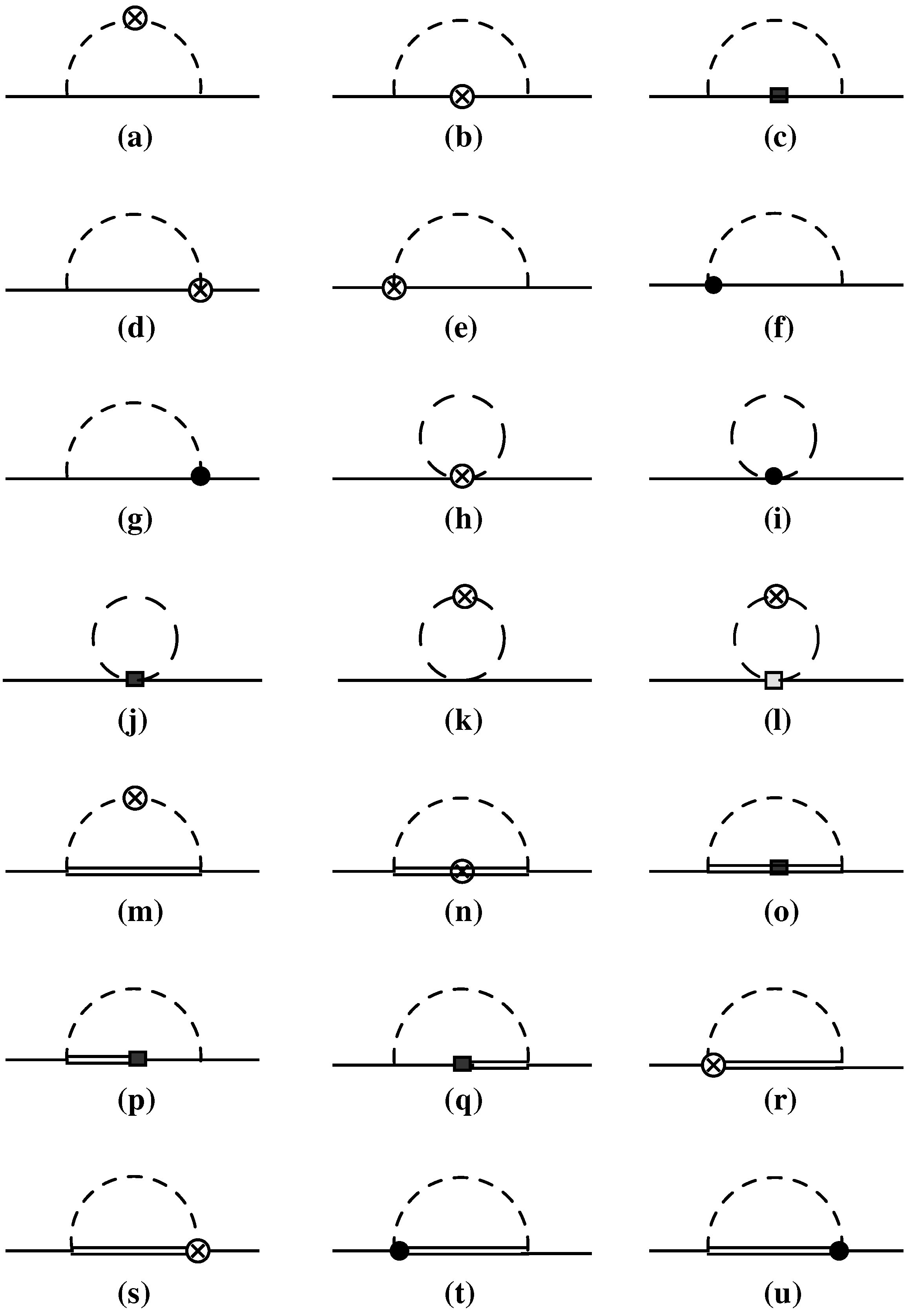
The diagrams relevant for the calculation of the one-meson loop contributions to the GPDs up to $\mathcal{O}\left(p^4\right)$ are depicted in Figure 1. Assuming that meson loop diagrams are the only source of antiquarks in the proton, the convolution formulas for the electric and magnetic contributions to the antiquark GPDs arise from Figure 1a,k–m. For the specific case of the $H^{\overline{q}}$ and $E^{\overline{q}}$ GPDs at $\xi =0$, one has

$$\begin{array}{ccc}\hfill H^{\overline{q}}(x,t)& =& \sum _{\varphi BT}\left[\left(f_{\varphi B}^{\left(\mathrm{rbw}\right)}+f_{\varphi T}^{\left(\mathrm{rbw}\right)}+f_{\varphi }^{\left(\mathrm{bub}\right)}\right)\otimes H_{\varphi }^{\overline{q}}\right](x,t),\hfill \end{array}$$

(40a)

$$\begin{array}{ccc}\hfill E^{\overline{q}}(x,t)& =& \sum _{\varphi BT}\left[\left(g_{\varphi B}^{\left(\mathrm{rbw}\right)}+g_{\varphi T}^{\left(\mathrm{rbw}\right)}+g_{\varphi }^{\prime \left(\mathrm{bub}\right)}\right)\otimes H_{\varphi }^{\overline{q}}\right](x,t),\hfill \end{array}$$

(40b)

where $H_{\varphi }^{\overline{q}}$ is the electric GPD for quark flavor $\overline{q}$ in the meson $\varphi$. The functions $f_{\varphi B}^{\left(\mathrm{rbw}\right)}$ and $g_{\varphi B}^{\left(\mathrm{rbw}\right)}$ are the splitting functions corresponding to rainbow diagram in Figure 1a, $f_{\varphi T}^{\left(\mathrm{rbw}\right)}$ and $g_{\varphi T}^{\left(\mathrm{rbw}\right)}$ are the decuplet recoil splitting functions corresponding to the rainbow diagrams in Figure 1m, and $f_{\varphi }^{\left(\mathrm{bub}\right)}$ and $g_{\varphi }^{\prime \left(\mathrm{bub}\right)}$ are the splitting functions corresponding to the bubble diagrams in Figure 1k and Figure 1l, respectively. The splitting functions are given explicitly by He et al. [121], and the symbol ⊗ represents the convolution in the parton momentum fraction with the GPD $H_{\varphi }^{\overline{q}}$ in the meson $\varphi$.

In contrast to the antiquark case, the quark GPDs receive contributions from all of the diagrams in Figure 1, resulting in a more complicated convolution structure,

$$\begin{array}{ccc}\hfill H^q(x,t)& =& Z_2{H}_0^q(x,t)+\sum _{\varphi BT}[\left(f_{\varphi B}^{\left(\mathrm{rbw}\right)}+f_{\varphi T}^{\left(\mathrm{rbw}\right)}+f_{\varphi }^{\left(\mathrm{bub}\right)}\right)\otimes H_{\varphi }^q\hfill \\ & & +{\overline{f}}_{B\varphi }^{\left(\mathrm{rbw}\right)}\otimes H_B^q+{\overline{f}}_{B\varphi }^{\left(\mathrm{KR}\right)}\otimes H_B^{q\left(\mathrm{KR}\right)}+\delta {\overline{f}}_B^{\left(\mathrm{KR}\right)}\otimes H_B^{q\left(\mathrm{KR}\right)}\hfill \\ & & +{\overline{f}}_{T\varphi }^{\left(\mathrm{rbw}\right)}\otimes H_T^q+{\overline{f}}_{T\varphi }^{\left(\mathrm{KR}\right)}\otimes H_T^{q\left(\mathrm{KR}\right)}+\delta {\overline{f}}_{T\varphi }^{\left(\mathrm{KR}\right)}\otimes H_T^{q\left(\mathrm{KR}\right)}\hfill \\ & & +{\overline{f}}_{B\varphi }^{\left(\mathrm{rbw}\mathrm{mag}\right)}\otimes E_B^q+{\overline{f}}_{T\varphi }^{\left(\mathrm{rbw}\mathrm{mag}\right)}\otimes E_T^q+{\overline{f}}_{BT}^{\left(\mathrm{rbw}\mathrm{mag}\right)}\otimes E_{BT}^q\hfill \\ & & +{\overline{f}}_{\varphi }^{\left(\mathrm{tad}\right)}\otimes H_{\varphi {\varphi }^{†}}^{q\left(\mathrm{tad}\right)}+\delta {\overline{f}}_{\varphi }^{\left(\mathrm{tad}\right)}\otimes H_{\varphi {\varphi }^{†}}^{q\left(\mathrm{tad}\right)}](x,t),\hfill \end{array}$$

(41a)

$$\begin{array}{ccc}\hfill E^q(x,t)& =& Z_2{E}_0^q(x,t)+\sum _{\varphi BT}[\left(g_{\varphi B}^{\left(\mathrm{rbw}\right)}+g_{\varphi T}^{\left(\mathrm{rbw}\right)}+g_{\varphi }^{\prime \left(\mathrm{bub}\right)}\right)\otimes H_{\varphi }^q\hfill \\ & & +{\overline{g}}_{B\varphi }^{\left(\mathrm{rbw}\right)}\otimes H_B^q+{\overline{g}}_{B\varphi }^{\left(\mathrm{KR}\right)}\otimes H_B^{q\left(\mathrm{KR}\right)}+\delta {\overline{g}}_B^{\left(\mathrm{KR}\right)}\otimes H_B^{q\left(\mathrm{KR}\right)}\hfill \\ & & +{\overline{g}}_{T\varphi }^{\left(\mathrm{rbw}\right)}\otimes H_T^q+{\overline{g}}_{T\varphi }^{\left(\mathrm{KR}\right)}\otimes H_T^{q\left(\mathrm{KR}\right)}+\delta {\overline{g}}_{T\varphi }^{\left(\mathrm{KR}\right)}\otimes H_T^{q\left(\mathrm{KR}\right)}\hfill \\ & & +{\overline{g}}_{B\varphi }^{\left(\mathrm{rbw}\mathrm{mag}\right)}\otimes E_B^q+{\overline{g}}_{T\varphi }^{\left(\mathrm{rbw}\mathrm{mag}\right)}\otimes E_T^q+{\overline{g}}_{BT}^{\left(\mathrm{rbw}\mathrm{mag}\right)}\otimes E_{BT}^q\hfill \\ & & +{\overline{g}}_{\varphi }^{\left(\mathrm{tad}\mathrm{mag}\right)}\otimes E_{\varphi {\varphi }^{†}}^{q\left(\mathrm{tad}\right)}](x,t),\hfill \end{array}$$

(41b)

where $H_0^q$ and $E_0^q$ are the quark GPDs of the bare proton, and the wave function renormalization constant $Z_2$ reflects the dressing of the bare proton by the meson loops. The additional splitting functions in Equation (41) corresponding to Figure 1b–j,n–u are given by He et al. [121]. Note that $\delta$-function terms appear in the splitting functions at zero momentum, which have contributions to the lowest moments of the GPDs but not to higher moments. As shorthand, in Equation (41), we use the notation ${\overline{f}}_j\left(y\right)\equiv f_j(1-y)$ and ${\overline{g}}_j\left(y\right)\equiv g_j(1-y)$ to represent the electric and magnetic splitting functions involving couplings to baryons. Note that both the electric and magnetic operators contribute to $H^q(x,t)$ and $E^q(x,t)$ at zero- and finite-momentum transfer. At zero-momentum transfer, however, the magnetic term does not contribute to the matrix element, even though the GPD $E^q(x,0)$ itself is nonzero.

The quark and antiquark GPDs in Equations (40) and (41) provide the foundation for computing meson loop contributions to GPD flavor asymmetries. The relevant intermediate states consist of nucleon and $\mathrm{\Delta }$ baryons with $\pi$ mesons for u and d quarks, and $\mathrm{\Lambda }$, $\mathrm{\Sigma }$, and ${\mathrm{\Sigma }}^{\ast }$ hyperons with K mesons for the strange quark. Numerical evaluation of these GPDs requires modeling the hadronic GPDs appearing in the convolution formulas. Following Refs. [36,121], we express these in terms of pion and proton GPDs, which are parametrized as products of valence parton distribution functions (PDFs) and t-dependent form factors [121,187]. Using the computed splitting functions and valence quark distributions as input, the sea quark GPDs are then evaluated from the convolution expressions in Equations (40) and (41).

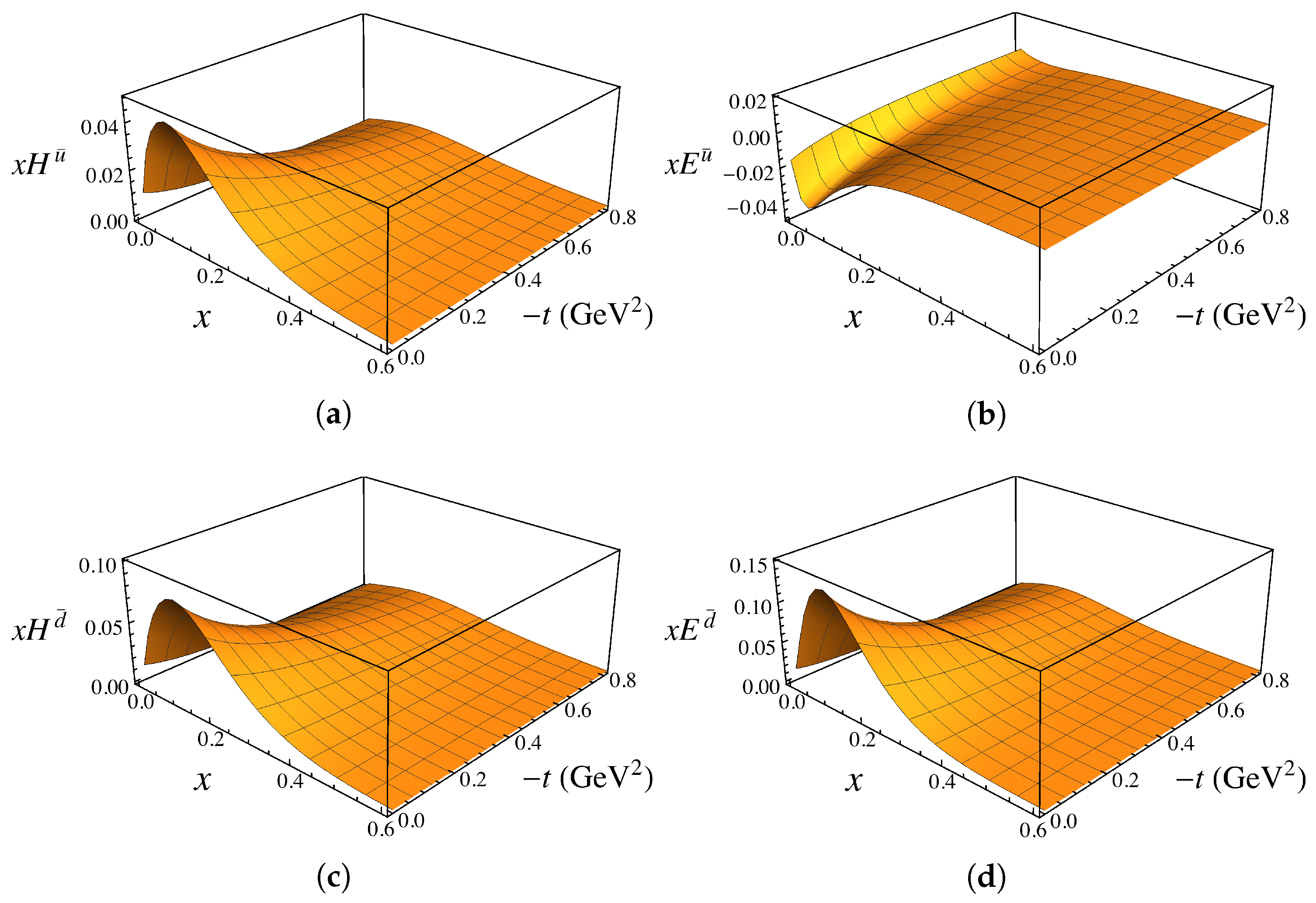
The electric ($H^{\overline{q}}$) and magnetic ($E^{\overline{q}}$) GPDs for light antiquarks in the proton, generated from meson loops, are presented in Figure 2 as functions of the parton momentum fraction x and momentum transfer $-t$ for $\overline{u}$ and $\overline{d}$ flavors at $Q=1$ GeV. For $\overline{u}$ antiquarks, the distribution $x{H}^{\overline{u}}$ is positive, peaking at $x\approx 0.1$, with little t dependence. At fixed x, its magnitude decreases monotonically with increasing $-t$. In contrast, the $x{E}^{\overline{u}}$ GPD is negative, peaks at slightly lower x, and its magnitude also decreases with $-t$. The $\overline{d}$ antiquark GPD $x{H}^{\overline{d}}$ exhibits a similar shape to $x{H}^{\overline{u}}$, but is systematically larger at all x and t values. This flavor asymmetry originates from the intermediate states involved, with $H^{\overline{d}}$ receiving contributions from both octet and decuplet baryons, but $H^{\overline{u}}$ arising solely from decuplet intermediate states.

The shapes of the magnetic $E^{\overline{q}}$ GPDs reflect the important role played by the orbital angular momentum of the mesons in the intermediate states. For octet baryon intermediate states, the meson orbital angular momentum is typically positive, which produces positive $E^{\overline{d}}$ values. In contrast, for $\overline{u}$ quarks, where only decuplet intermediate states contribute, the meson orbital angular momentum tends to be negative, resulting in negative values for $E^{\overline{u}}$. The magnitude of $x{E}^{\overline{d}}$ is also much larger than that of $x{E}^{\overline{u}}$. Note that the $\delta$-function term in the splitting functions does not contribute to the $H^{\overline{q}}$ and $E^{\overline{q}}$ GPDs, although it does contribute to the lowest moments of these functions.

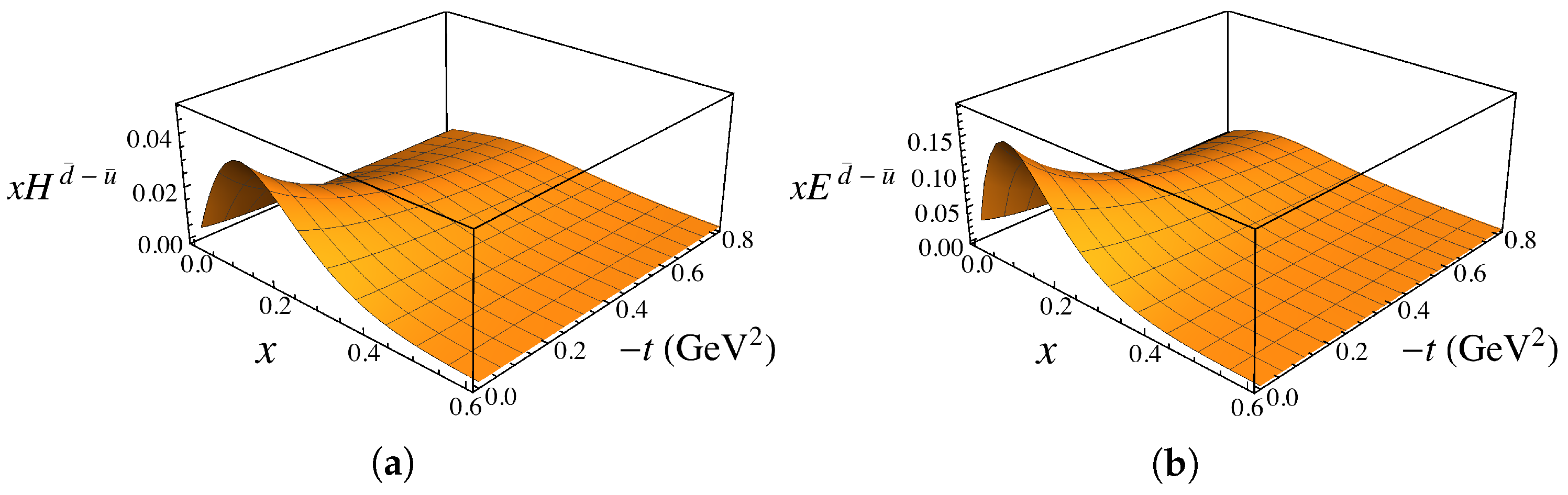
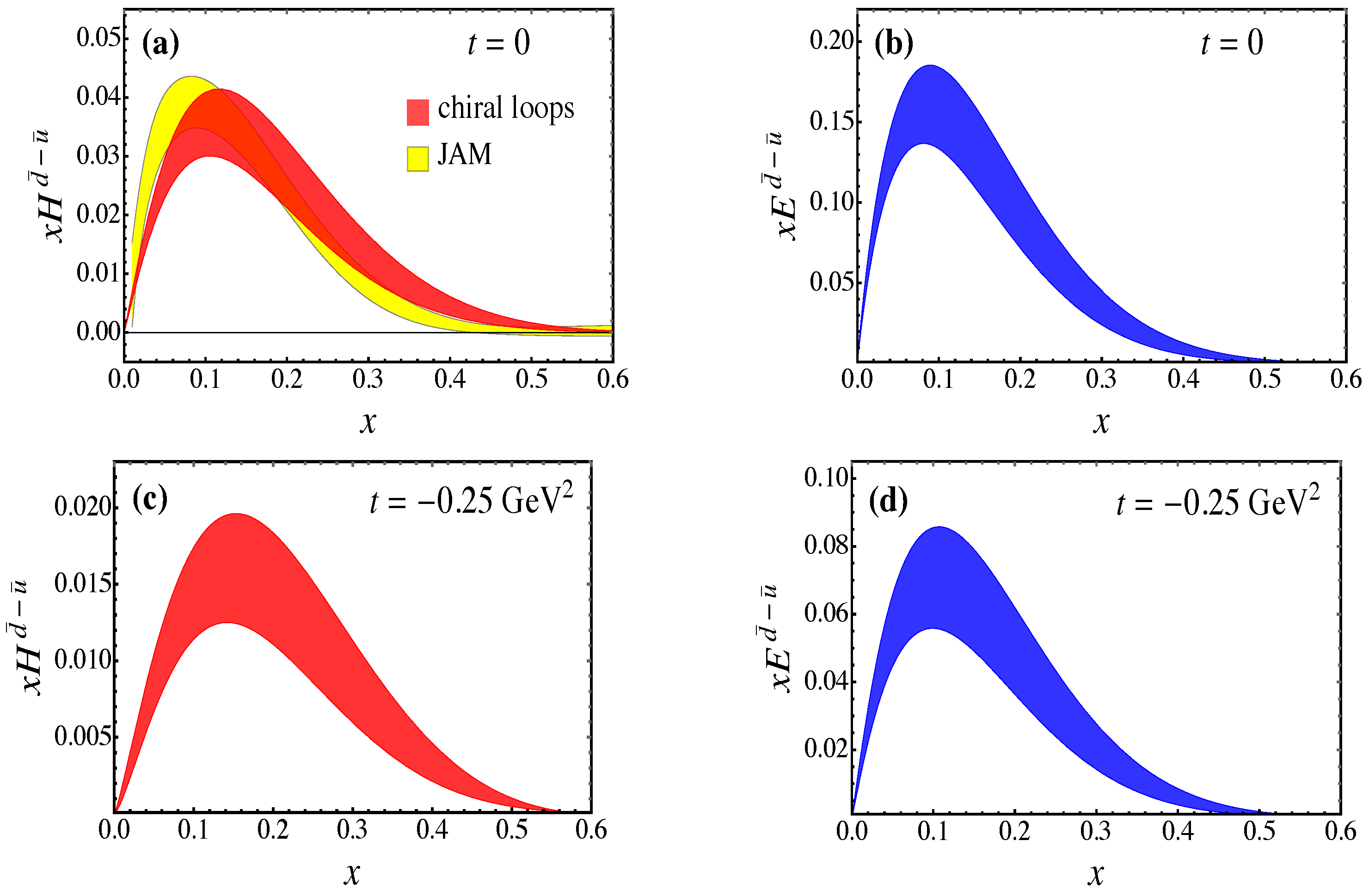
The light-flavor GPDs asymmetries, $x{H}^{\overline{d}-\overline{u}}$ and $x{E}^{\overline{d}-\overline{u}}$, are shown in Figure 3 as functions of x and $-t$. Both asymmetries are positive across all x values, peaking at $x\approx 0.1$ and decreasing with increasing $-t$. Notably, at the peak, the magnetic asymmetry $x{E}^{\overline{d}-\overline{u}}$ is approximately 4 times larger than the electric asymmetry $x{H}^{\overline{d}-\overline{u}}$. To more clearly illustrate the shape of the $\overline{d}-\overline{u}$ asymmetry, in Figure 4, we show the electric $x{H}^{\overline{d}-\overline{u}}$ and magnetic $x{E}^{\overline{d}-\overline{u}}$ distributions at $t=0$, with uncertainty bands reflecting a 10% variation in the cutoff parameter, $\mathrm{\Lambda }=1.0\left(1\right)$ GeV. The calculated electric asymmetry compares well with the recent JAM global QCD analysis [188] at $Q=1.3$ GeV, which finds a maximum of $\approx 0.3-0.4$ at $x\approx 0.05-0.10$, driven largely by Drell-Yan proton–proton and proton–deuteron scattering data [23,24]. Integrating over x, the lowest moments of the electric GPD asymmetry are ${\int }_0^{1}dx{H}^{\overline{d}-\overline{u}}(x,0)=0.11\left(2\right)$ and ${\int }_0^{1}dxx{H}^{\overline{d}-\overline{u}}(x,0)=0.009\left(2\right)$, where the uncertainties correspond to the $\mathrm{\Lambda }$ variation. The magnetic asymmetry $x{E}^{\overline{d}-\overline{u}}$ at $t=0$ has a similar shape but is approximately 4 times larger than the electric asymmetry at the peak, consistent with large-$N_c$ QCD predictions [189]. Its integrated moments are found to be ${\int }_0^{1}dx{E}^{\overline{d}-\overline{u}}(x,0)=1.1\left(2\right)$ and ${\int }_0^{1}dxx{E}^{\overline{d}-\overline{u}}(x,0)=0.034\left(6\right)$. The large magnitude of the magnetic asymmetry provides an opportunity for its determination in future experiments.

The $x{H}^{\overline{d}-\overline{u}}$ and $x{E}^{\overline{d}-\overline{u}}$ GPD asymmetries at finite t, $-t=0.25$ GeV², are displayed in Figure 4. As expected from the 3-dimensional distributions in Figure 3, both asymmetries are suppressed at finite t values, with magnitudes reduced to approximately half of the $t=0$ values. This suppression is consistent with the GPD inequality $H^q(x,t)\le H^q(x,0)$ [190,191]. Additionally, the peaks of both distributions shift slightly toward larger x values with increasing $-t$.

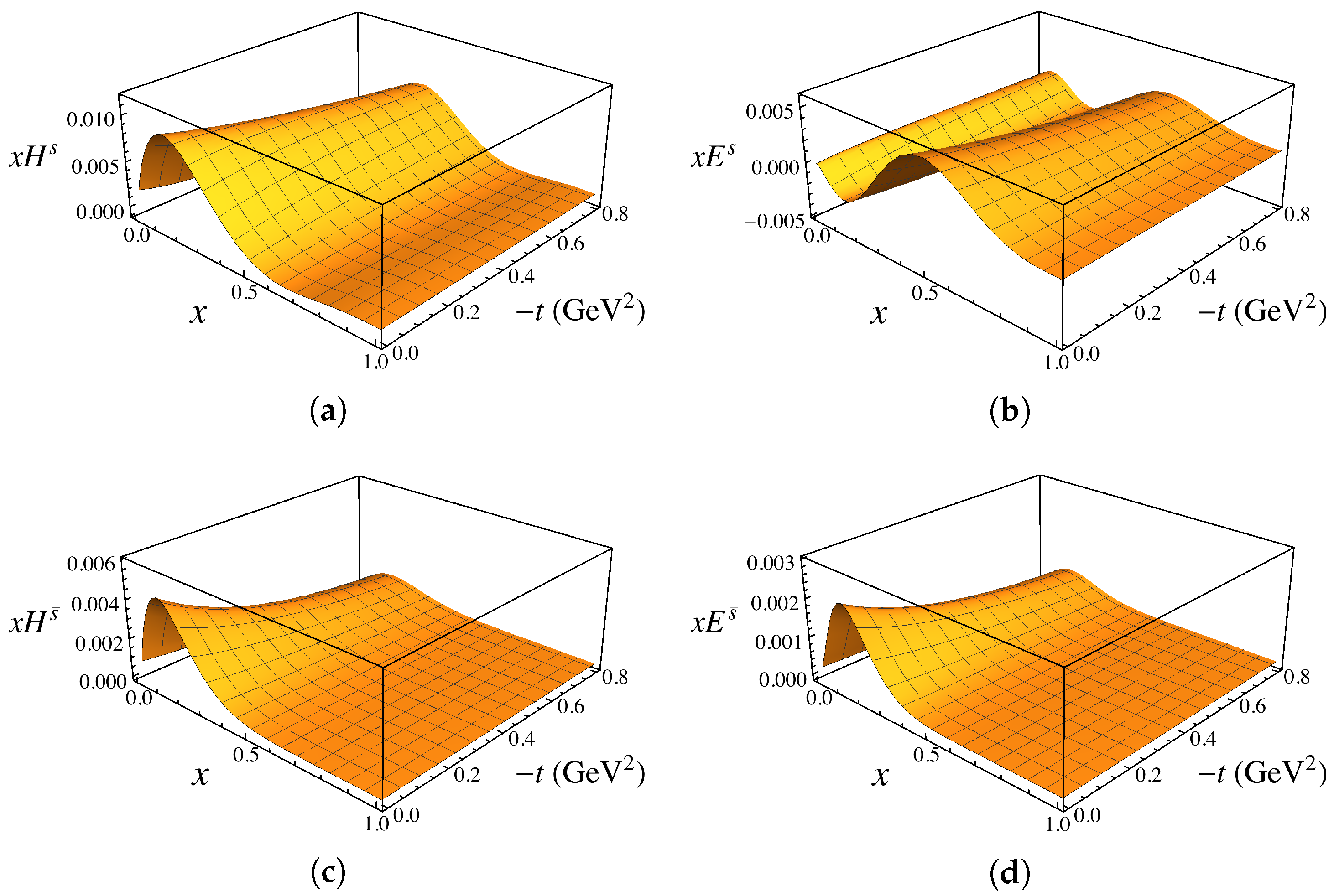
The kaon loop contributions to the strange quark GPDs are shown in Figure 5. Although smaller in magnitude than their light antiquark counterparts, the strange GPDs exhibit several notable features. As for the light antiquarks, the strange electric GPDs $H^s$ and $H^{\overline{s}}$ are both positive. Perturbatively, the s and $\overline{s}$ distributions are expected to be nearly identical [192]; however, their kaon loop contributions differ significantly due to their distinct origins. Under the assumption of SU(3) flavor symmetry for the intermediate state GPDs [36,121], the $\overline{s}$ antiquark GPD arises from direct couplings to the kaon [Figure 1a], whereas the s quark GPD arises from couplings to intermediate hyperons [Figure 1b] [193,194].

As shown in Figure 5, the strange $H^s$ GPD exceeds the antistrange $H^{\overline{s}}$ at small x, while this hierarchy reverses at larger x values, namely $x\gtrsim 0.5$. At $t=0$, the x-integrals of $H^s$ and $H^{\overline{s}}$ are equal when including the $\delta$-function term, ensuring zero net strangeness in the nucleon. However, their different t dependence leads to unequal lowest moments at finite t, corresponding to a nonzero strange electric form factor for $-t>0$. The magnetic GPDs $E^s$ and $E^{\overline{s}}$ exhibit more complex behavior, on the other hand. The antistrange $E^{\overline{s}}$ is positive, similar to $E^{\overline{d}}$, due to positive meson orbital angular momentum. In contrast, the strange $E^s$ changes sign with x, from negative at small x values to positive at large x values, $x\gtrsim 0.3$.

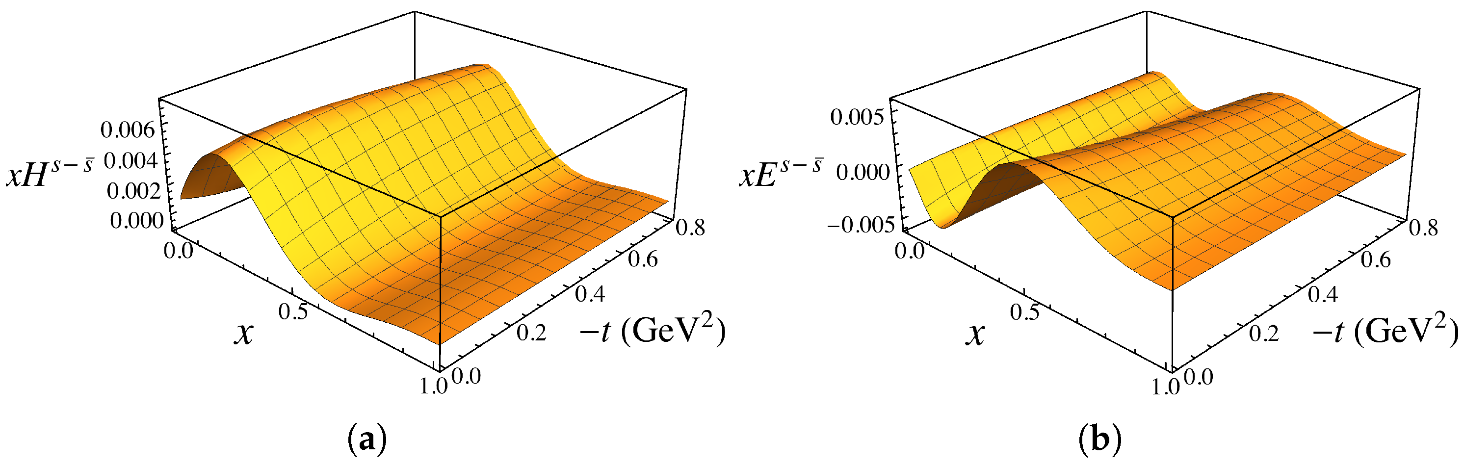
The strange–antistrange asymmetries $x{H}^{s-\overline{s}}$ and $x{E}^{s-\overline{s}}$ are displayed in Figure 6 as functions of x and $-t$ for $\mathrm{\Lambda }=1$ GeV. For the electric asymmetry, $x{H}^{s-\overline{s}}$ is generally positive at nonzero x, peaking at $x\approx 0.2-0.3$. Unlike the individual s and $\overline{s}$ GPDs, the asymmetry does not decrease monotonically with $-t$ and, in some regions, even increases at higher momentum transfers. The magnetic asymmetry $x{E}^{s-\overline{s}}$ exhibits a sign change with x, driven by the behavior of $x{E}^s$. Overall, both the electric and magnetic $s-\overline{s}$ asymmetries are significantly smaller than the corresponding light quark $\overline{d}-\overline{u}$ asymmetries in the nucleon.

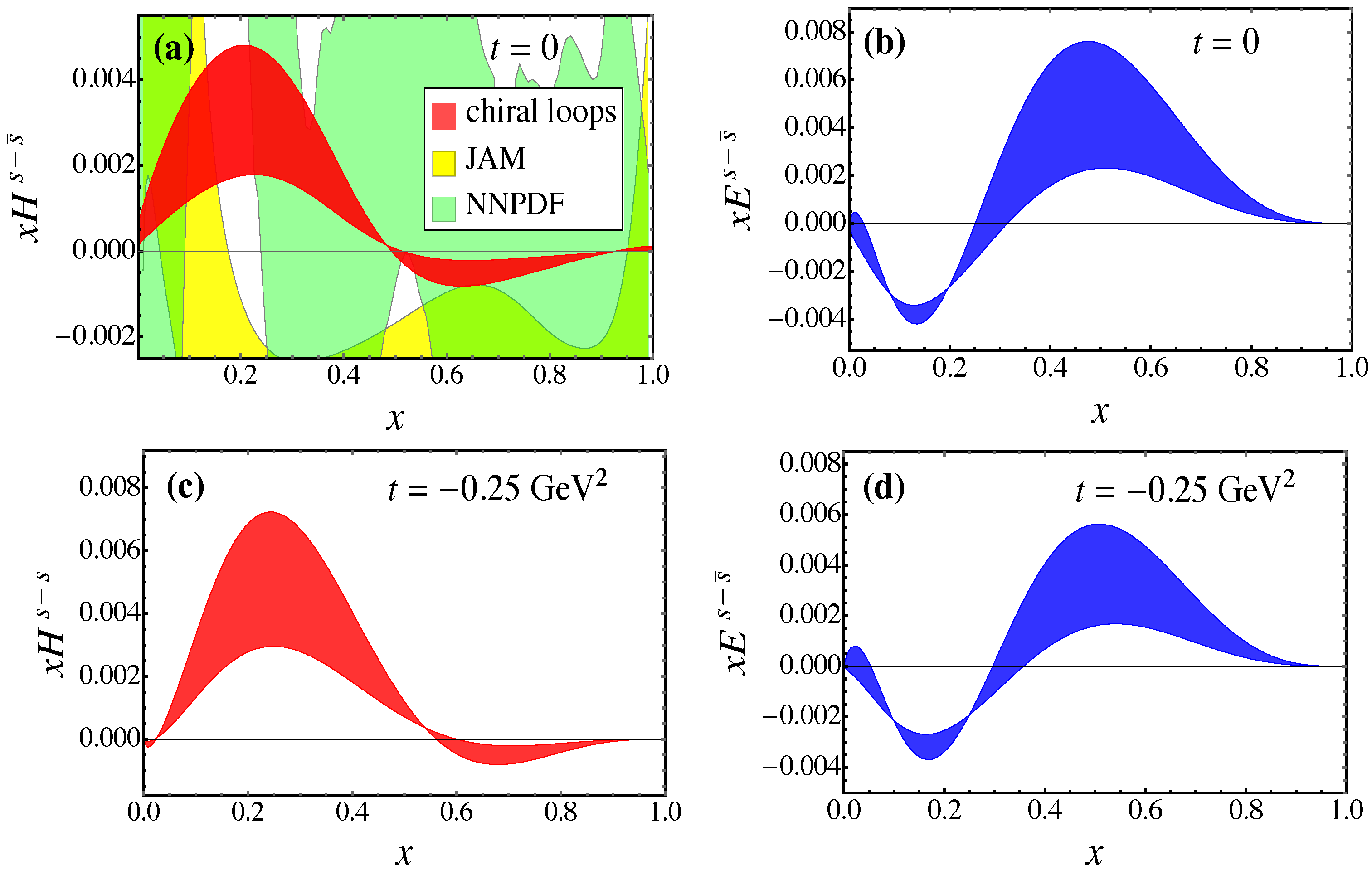
In analogy with the $\overline{d}-\overline{u}$ asymmetry in Figure 4, in Figure 7, we display the $s-\overline{s}$ asymmetries $x{H}^{s-\overline{s}}$ and $x{E}^{s-\overline{s}}$ at $t=0$ and $-t=0.25$ GeV² for cutoffs $\mathrm{\Lambda }=(0.9-1.1)$ GeV. The electric asymmetry $x{H}^{s-\overline{s}}$ changes sign, from positive at small x to negative at $x\gtrsim 0.5$. Comparison with JAM [188] and NNPDF [195] PDF parametrizations reveals substantial uncertainties in the experimental extractions relative to the theoretical estimate. For the lowest nonzero moment of the electric asymmetry, one obtains ${\int }_0^{1}dxx{H}^{s-\overline{s}}(x,0)=0.{0009}_{\left(4\right)}^{\left(5\right)}$, consistent with other phenomenological estimates [36,111,196]. For the magnetic asymmetry $x{E}^{s-\overline{s}}$, the sign behavior is reversed, with the asymmetry being negative at small x and positive for $x\gtrsim 0.3$. The corresponding moments are found to be ${\int }_0^{1}dxx{E}^{s-\overline{s}}(x,0)=0.{0009}_{\left(8\right)}^{\left(12\right)}$ and ${\int }_0^{1}dx{E}^{s-\overline{s}}(x,0)\equiv {\mu }_s=-0.{033}_{\left(13\right)}^{\left(11\right)}$, where ${\mu }_s$ represents the strange quark contribution to the proton’s magnetic moment.

At finite momentum transfers t, the strange asymmetry exhibits significantly less suppression than the nonstrange $\overline{d}-\overline{u}$ asymmetry. As shown in Figure 7, for $-t=0.25$ GeV², the magnetic GPD asymmetry $x{E}^{s-\overline{s}}(x,t)$ is only slightly reduced relative to its $t=0$ value. Interestingly, for the electric GPD asymmetry, the peak magnitude of $x{H}^{s-\overline{s}}(x,t)$ at $-t=0.25$ GeV² actually exceeds that at $t=0$.

2.4. GPDs with Nonzero Skewness

In this section, we extend the previous analysis of zero-skewness GPDs in the proton [121] to the case of nonzero skewness. As an initial step toward a complete one-loop calculation, this analysis considers the contributions to the sea quark and antiquark GPDs from the virtual pseudoscalar meson cloud that dresses the bare baryon. Typically, in calculations of meson loop contributions to sea quark asymmetries [35], one assumes that the undressed proton contains a flavor-symmetric sea [35], so that differences between sea quark and antiquark PDFs and GPDs arise exclusively from the meson coupling diagrams in Figure 1a,k–m.

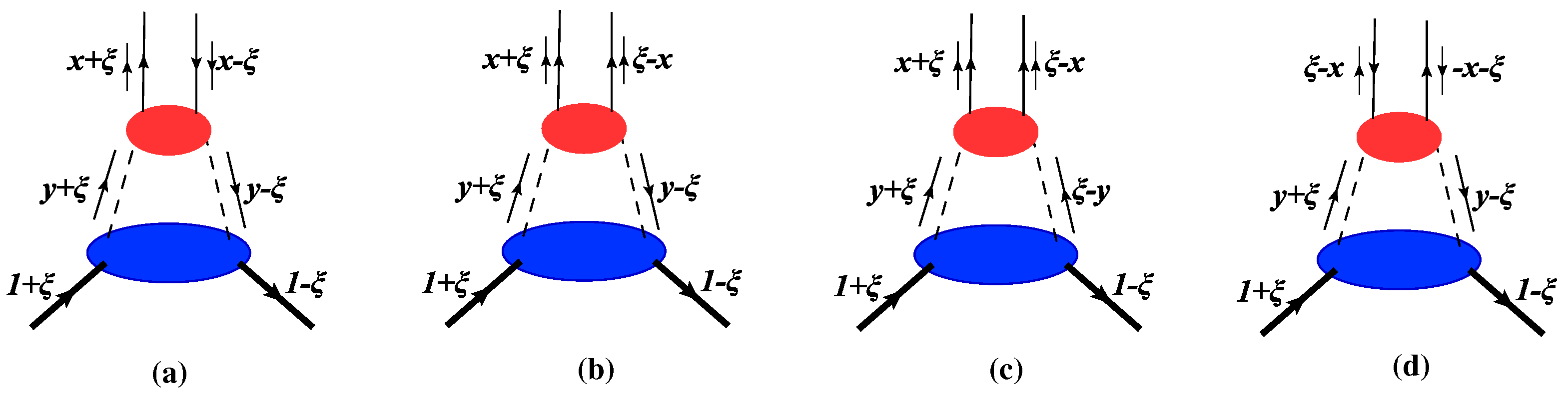
For the rainbow diagrams in Figure 1a,m, the splitting functions are nonzero for $-\xi \le y\le 1$ with $\xi >0$. The splitting functions in this region can be convoluted with the pion GPD to obtain the quark GPD in the physical nucleon. The decomposition of the convolution for the rainbow diagram in Figure 1a is illustrated in Figure 8. The splitting functions in Figure 8a,b,d correspond to $y>\xi$ and, when convoluted with the pion GPD, map to the quark Dokshitzer–Gribov–Lipatov–Altarelli–Parisi (DGLAP) [197,198,199], Efremov–Radyushkin–Brodsky–Lepage (ERBL) [200,201,202], and antiquark DGLAP regions of the proton GPD, respectively. For the subprocess in Figure 8c, the splitting function is defined in the range $y\in [-\xi ,\xi ]$, representing a meson–meson pair annihilation analogous to quark-level distribution amplitude dynamics.

By combining these various processes, the contribution to the nonzero-skewness GPDs from the diagram in Figure 1a can be expressed in the convolution form as

$$H_q^{\left(\mathrm{rbw}\right)}(x,\xi ,t)=\{\begin{array}{}\mathrm{(42a)}& {\int }_x^1{\displaystyle \frac{dy}{y}}{f}_{\varphi B}^{\left(\mathrm{rbw}\right)}(y,\xi ,t)H_{q/\varphi }\left({\displaystyle \frac{x}{y}},{\displaystyle \frac{\xi }{y}},t\right),\hfill & [\xi <x<y]\mathrm{(42b)}& {\int }_{\xi }^1{\displaystyle \frac{dy}{y}}{f}_{\varphi B}^{\left(\mathrm{rbw}\right)}(y,\xi ,t)H_{q/\varphi }\left({\displaystyle \frac{x}{y}},{\displaystyle \frac{\xi }{y}},t\right),\hfill & [x<\xi <y]\mathrm{(42c)}& {\int }_{-\xi }^{\xi }{\displaystyle \frac{dy}{2y}}{f}_{\varphi B}^{\left(\mathrm{rbw}\right)}(y,\xi ,t){\displaystyle \frac{1}{\pi }}{\int }_{s_0}^{\infty }ds{\displaystyle \frac{\mathrm{Im}{\mathrm{\Phi }}_{q/\varphi }\left(\frac{1}{2}(1+\frac{x}{\xi }),\frac{1}{2}(1+\frac{y}{\xi }),s\right)}{s-t+iϵ}},\hfill & \left[\right|x|,|y|<\xi ]\mathrm{(42d)}& {\int }_{-x}^1{\displaystyle \frac{dy}{y}}{f}_{\varphi B}^{\left(\mathrm{rbw}\right)}(y,\xi ,t)H_{q/\varphi }\left({\displaystyle \frac{x}{y}},{\displaystyle \frac{\xi }{y}},t\right),\hfill & [\xi <-x<y<1]\end{array}$$

where $H_{q/\varphi }$ and ${\mathrm{\Phi }}_{q/\varphi }$ are the valence GPD and generalized distribution amplitude (GDA) of the intermediate pseudoscalar meson, respectively. The integration variable $s={(2k_{\varphi }+\mathrm{\Delta })}^2$ in Equation (42c) represents the four-momentum squared of the produced meson pair with momentum $k_{\varphi }$ and $k_{\varphi }+\mathrm{\Delta }$, with threshold value $s_0={\left(2m_{\varphi }\right)}^2$.

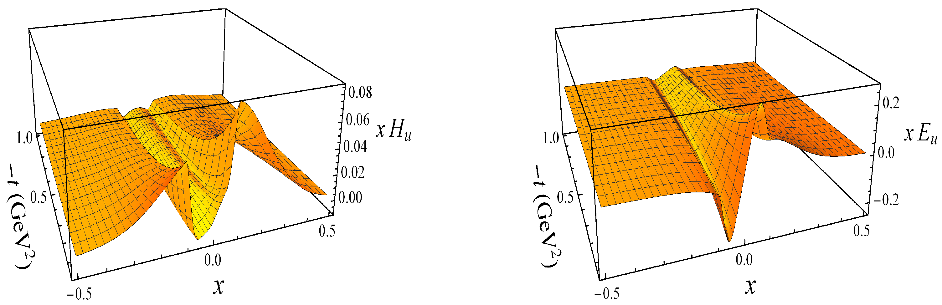
The chiral loop contributions to the u-quark H and E GPDs, obtained by convoluting the splitting functions with the virtual pion GPDs as in Equation (42), are shown in Figure 9 at fixed $\xi =0.1$. For the pion loop diagrams in Figure 1a,k–m, the d-quark GPDs follow from isospin symmetry, ${\{H,E\}}_d(x,\xi ,t)=-{\{H,E\}}_u(-x,\xi ,t)$. The most prominent features appear at $\left|x\right|\lesssim 0.2$. The electric GPD $x{H}_u$ is positive in the DGLAP region and displays two valleys in the ERBL region. Conversely, the magnetic GPD $x{E}_u$ is negative for $x<0$ and positive for $x>0$. Both distributions decrease rapidly as $\left|x\right|\to 1$ and with increasing $-t$.

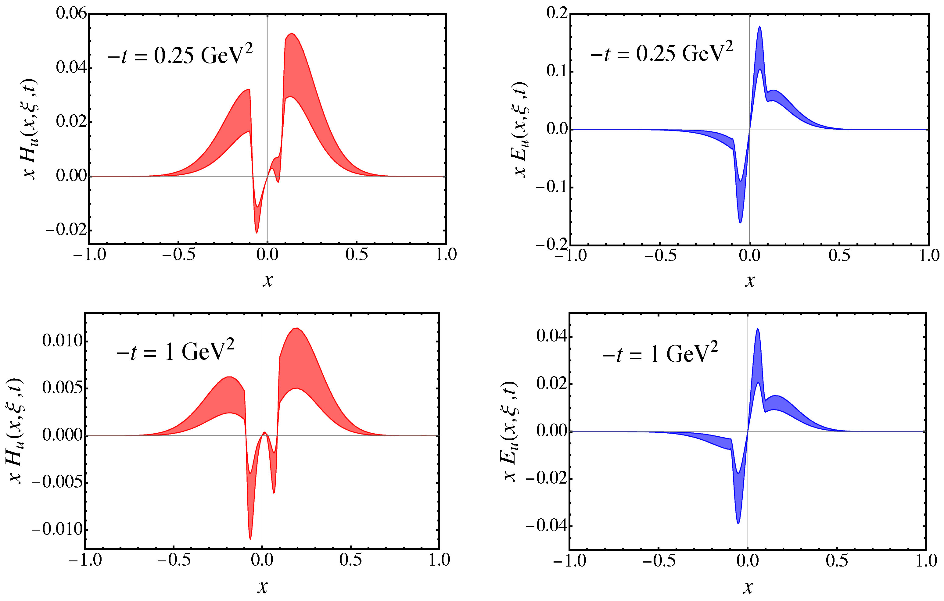
To more clearly illustrate the x dependence of the GPDs, Figure 10 shows the two-dimensional projections of $x{H}_u$ and $x{E}_u$ at $-t=0.25$ GeV² and $-t=1$ GeV². Although the splitting function $f_{{\pi }^{+}{\mathrm{\Delta }}^0}^{\left(\mathrm{rbw}\right)}$ is discontinuous at $y=\xi$, the quark GPDs remain continuous at the ridge $x=\pm \xi$. This continuity arises from the fact that the convolution formulas in Equations (42a), (42b) and (42d) involve only the $y>\xi$ region, and they yield continuous results at $x=\xi$ when the input pion GPD is continuous, which guarantees finite amplitudes for DVCS and hard exclusive meson production [203]. No such constraints apply, however, to the GPD derivatives at $x=\xi$. Discontinuity of the derivative can arise from different integration regions in the $\alpha$–$\beta$ plane for the DGLAP and ERBL regimes within the double distribution parametrization [203,204]. Additionally, the D-term contribution, which is confined to the ERBL region, also induces a first-derivative discontinuity at $x=\xi$. On the other hand, the contribution to the quark GPD from Equation (42c) vanishes at $x=\xi$ due to the endpoint behavior of the distribution amplitude, ${\mathrm{\Phi }}_{q/\pi }(1,\kappa ,s)=0$, where $\kappa =p^{\prime +}/(p^{+}+p^{\prime +})$.

Comparing the results at different $-t$ values, the magnitudes of the GPD at $-t=0.25$ GeV² are approximately 4-5 times larger than those at $-t=1$ GeV². For the u-quark distribution, the quark GPD $H_u$ in the DGLAP region ($x>0$) has greater magnitude than at $x<0$ (equivalent to $\overline{u}$ at $x>0$ by crossing symmetry). From the isospin relation for the pion coupling diagrams, the u-quark GPD $x{H}_u(x>0)$ is equivalent to the d-quark GPD $x{H}_d(x<0)$, which corresponds to the $\overline{d}$ distribution at $x>0$. Consequently, the loop diagrams in Figure 1a,k–m naturally produce an enhanced $\overline{d}$ distribution relative to $\overline{u}$, reminiscent of the empirical $\overline{d}/\overline{u}$ asymmetry observed for collinear PDFs [35].

Furthermore, the GPD in the $0<x<\xi$ region is positive at $-t=0.25$ GeV², but negative at $-t=1$ GeV². This sign can be understood because the pion GPD (or GDA) in the ERBL region incorporates the $D_{q/\pi }\left(t\right)$ form factor, which exhibits different t dependence than the pion form factor $F_{\pi }\left(t\right)$. The magnetic GPD $E_u$ has a larger magnitude than the electric $H_u$, and the quark and antiquark distributions in the DGLAP region have opposite signs. This implies that the electric GPD for $\overline{u}$ has the opposite sign to that for $\overline{d}$, while the magnetic GPD E for $\overline{d}$ is larger in magnitude than for $\overline{u}$.

3. Nonlocal QED

The second example of an application of nonlocal field theory methods that we discuss in this review is the generalization of QED to the most general nonlocal interaction. As for the application to hadronic interactions, nonlocal behavior is also expected in fundamental interactions, such as between electrons and photons. Although the nonlocal effects here are generally less pronounced than in the hadronic sector, they can be tested if the measured quantity is sufficiently accurate. We begin with some basics about the nonlocal QED Lagrangian, followed by a discussion of solid quantization and gauge invariance, before focusing on the specific problem of the $g-2$ anomaly.

3.1. Nonlocal QED Lagrangian

In this section, we introduce the general extension of the local QED Lagrangian, where both the free and interacting parts are nonlocal [123,124], and present the Feynman rules for vertices, including the additional interaction generated from gauge links. Recall that the local QED Lagrangian is given by

$${\mathcal{L}}^{\mathrm{local}}=\overline{\psi }\left(x\right)\left(i\cancel{\partial }-m\right)\psi \left(x\right)-e\overline{\psi }\left(x\right)\cancel{A}\left(x\right)\psi \left(x\right)-{\displaystyle \frac{1}{4}}{F}^{\mu \nu }\left(x\right)F_{\mu \nu }\left(x\right).$$

(43)

Based on the same $U\left(1\right)$ symmetry, the local QED Lagrangian can be transformed into a nonlocal Lagrangian using the method described in Refs. [36,113,115,116,117,118,119,120,121,122,123,124,181,184,205]. The most general nonlocal Lagrangian can be written as

$$\begin{array}{cc}\hfill {\mathcal{L}}^{\mathrm{nl}}& =\int d^{4}a\overline{\psi }\left(x+\frac{1}{2}a\right)I\left(x+\frac{1}{2}a,x\right)\left(i\cancel{\partial }-m\right)\psi \left(x-\frac{1}{2}a\right)I\left(x,x-\frac{1}{2}a\right)F_1\left(a\right)\hfill \\ \hfill -& e\int d^{4}a{d}^{4}b\overline{\psi }\left(x+\frac{1}{2}a\right)I\left(x+\frac{1}{2}a,x\right)\cancel{A}(x+b)\psi \left(x-\frac{1}{2}a\right)I\left(x,x-\frac{1}{2}a\right)F_1\left(a\right)F_2(a,b)\hfill \\ \hfill -& {\displaystyle \frac{1}{4}}\int d^{4}d{F}^{\mu \nu }\left(x\right)F_{\mu \nu }(x+d)F_4\left(d\right),\hfill \end{array}$$

(44)

where the gauge link,

$$I(x,y)\equiv exp\left(ie\int d^{4}c{\int }_x^{y}d{z}^{\mu }{A}_{\mu }(z+c)F_3(a,c)\right),$$

(45)

is introduced to guarantee local gauge invariance. In the nonlocal Lagrangian (44), the fermion fields $\psi$ and $\overline{\psi }$ are located at spacetime coordinates $x-\frac{1}{2}a$ and $x+\frac{1}{2}a$, respectively, while the photon field $A_{\mu }$ is located at $x+b$. The functions $F_1\left(a\right)$, $F_2(a,b)$, $F_3(a,c)$, and $F_4\left(d\right)$ are the correlation functions, normalized according to

$$\int d^{4}a{F}_1\left(a\right)=\int d^{4}b{F}_2(a,b)=\int d^{4}c{F}_3(a,c)=\int d^{4}d{F}_4\left(d\right)=1,$$

(46)

where we note the independence of a after the integration over b or c for the functions of $F_2(a,b)$ and $F_3(a,c)$, respectively. In the limits where $F_1\left(a\right)=\delta \left(a\right)$, $F_2(a,b)=\delta \left(b\right)$ and $F_4\left(d\right)=\delta \left(d\right)$, the nonlocal Lagrangian ${\mathcal{L}}^{\mathrm{nl}}$ reduces to the local Lagrangian ${\mathcal{L}}^{\mathrm{local}}$. It is straightforward to show that the most general nonlocal QED Lagrangian (44) is invariant under the gauge transformation

$$\begin{array}{ccc}\hfill \psi \left(x\right)& \to & e^{i\alpha \left(x\right)}\psi \left(x\right),\hfill \end{array}$$

(47a)

$$\begin{array}{ccc}\hfill A_{\mu }\left(x\right)& \to & A_{\mu }\left(x\right)-{\displaystyle \frac{1}{e}}{\partial }_{\mu }{\alpha }^{\prime }\left(x\right),\hfill \end{array}$$

(47b)

where

$$\alpha \left(x\right)=\int d^{4}b{\alpha }^{\prime }(x+b)F_2(a,b)=\int d^{4}c{\alpha }^{\prime }(x+c)F_3(a,c).$$

(48)

Note here that $\alpha \left(x\right)={\alpha }^{\prime }\left(x\right)$ in the local limit.

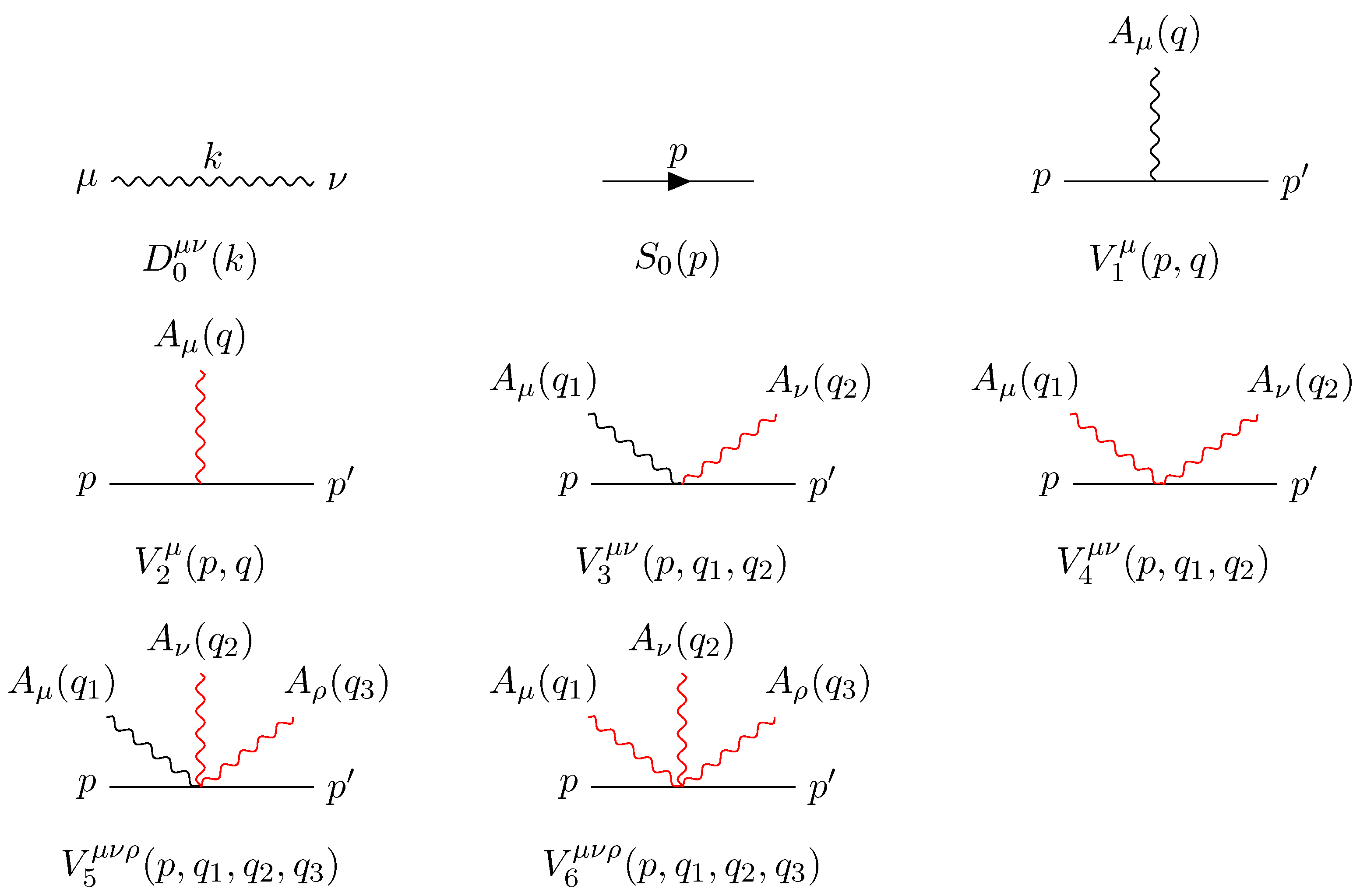
From the nonlocal Lagrangian (44), one can derive the corresponding Feynman rules. The propagators and vertices are illustrated in Figure 11, where, in addition to photons generated from the minimal substitution, one also has photons arising from the gauge links. Unlike the minimal substitution, which can only generate one photon, two or more photons can be obtained from the gauge link, so that the vertices in nonlocal QED can involve more than one photon. The free fermion and photon propagators in nonlocal QED are therefore modified according to

$$\begin{array}{ccc}\hfill S_0\left(p\right)& =& \left({\displaystyle \frac{i}{\cancel{p}-m}}\right){\displaystyle \frac{1}{{\tilde{F}}_1\left(p\right)}},\hfill \end{array}$$

(49a)

$$\begin{array}{ccc}\hfill D_0^{\mu \nu }\left(k\right)& =& \left({\displaystyle \frac{-i{g}^{\mu \nu }}{k^2}}\right){\displaystyle \frac{1}{{\tilde{F}}_4\left(k\right)}},\hfill \end{array}$$

(49b)

where the functions ${\tilde{F}}_1\left(p\right)$ and ${\tilde{F}}_4\left(k\right)$ are Fourier transformations of the correlation functions $F_1\left(a\right)$ and $F_4\left(d\right)$, respectively. In practice, the Feynman gauge is chosen for the calculation. The Gupta–Bleuler procedure works in the same way for the nonlocal theory as it does for local QED, and guarantees the equivalence of physical processes described in different gauges. The fermion–photon interaction term in the nonlocal Lagrangian ${\mathcal{L}}^{\mathrm{nl}}$ generated from the minimal substitution is given by $\int d^{4}a{d}^{4}b\overline{\psi }\left(x+\frac{1}{2}a\right)\cancel{A}(x+b)\psi \left(x-\frac{1}{2}a\right)F_1\left(a\right)F_2(a,b)$. The corresponding interaction vertex is

$$V_1^{\mu }(p,q)={\gamma }^{\mu }\int {\displaystyle \frac{d^{4}k}{{\left(2\pi \right)}^4}}{\tilde{F}}_1\left(k\right){\tilde{F}}_2\left({\displaystyle \frac{p+p^{\prime }}{2}}-k,q\right)={\gamma }^{\mu }{\tilde{G}}_2(p,q),$$

(50)

where q, p, and $p^{\prime }$ are the photon, initial fermion, and final fermion momenta, respectively, and ${\tilde{G}}_i(p,q)$ is defined as

$${\tilde{G}}_i(p,q)\equiv {\tilde{G}}_i(P,q)=\int {\displaystyle \frac{d^{4}k}{{\left(2\pi \right)}^4}}{\tilde{F}}_1\left(k\right){\tilde{F}}_i(P-k,q)(i=2,3),$$

(51)

with $P\equiv (p+p^{\prime })/2$.

In addition to the usual local QED interactions, the nonlocal Lagrangian ${\mathcal{L}}^{\mathrm{nl}}$ introduces additional interactions involving photons generated from the gauge link (45). The method for deducing the Feynman rules for these vertices was discussed in Refs. [113,181,184,205]. The related action for the interaction with one photon from the gauge link can be written as

$$S=-ie\int d^{4}a{d}^{4}c{d}^{4}x\overline{\psi }\left(x+\frac{1}{2}a\right)G_3(a,c)\left(i{\cancel{\partial }}_x-m\right)\psi \left(x-\frac{1}{2}a\right)I\left(x-\frac{1}{2}a,x+\frac{1}{2}a\right),$$

(52)

where $G_3(a,c)=F_1\left(a\right)F_3(a,c)$ and $I\left(x-\frac{1}{2}a,x+\frac{1}{2}a\right)={\int }_{x-\frac{1}{2}a}^{x+\frac{1}{2}a}d{z}^{\mu }{A}_{\mu }(z+c)$. To obtain the Feynman rule for this vertex requires calculating $\int d^{4}a{d}^{4}c{G}_3(a,c)e^{iPa}I\left(x-\frac{1}{2}a,x+\frac{1}{2}a\right)$. Using the identity

$$\begin{array}{ccc}& & \int d^{4}a{d}^{4}c{G}_3(a,c)e^{iPa}I\left(x-\frac{1}{2}a,x+\frac{1}{2}a\right)\hfill \\ \hfill & =& \int d^{4}a{d}^{4}c{d}^4{k}_1{d}^4{k}_2{\tilde{G}}_3(k_1,k_2)e^{i{k}_{1}a}{e}^{i{k}_{2}c}{e}^{iPa}I\left(x-\frac{1}{2}a,x+\frac{1}{2}a\right)\hfill \\ \hfill & =& \int d^{4}a{d}^{4}c{d}^4{k}_1{d}^4{k}_2\left({\tilde{G}}_3(-i{\partial }_a,k_2)e^{i{k}_{1}a}\right)e^{i{k}_{2}c}{e}^{iPa}I\left(x-\frac{1}{2}a,x+\frac{1}{2}a\right)\hfill \end{array}$$

(53)

and performing partial integration, one can show that [113,181,184]

$${\tilde{G}}_3(-i{\partial }_a,k_2)e^{iPa}I\left(x-\frac{1}{2}a,x+\frac{1}{2}a\right)=e^{iPa}{\tilde{G}}_3(-i{\mathcal{D}}_a,k_2)I\left(x-\frac{1}{2}a,x+\frac{1}{2}a\right),$$

(54)

where ${\mathcal{D}}_a={\partial }_a+i{P}_a$. Taylor expanding and using the iteration method [113,181,184,205], one can then write

$$\begin{array}{ccc}\hfill {\tilde{G}}_3(-i{\partial }_a,k_2)I\left(x-\frac{1}{2}a,x+\frac{1}{2}a\right)& =& i\int d^{4}q{\displaystyle \frac{(P^{\mu }+q^{\mu }/2)}{(2P·q+q^2)}}\left({\tilde{G}}_3(p+q,q)-{\tilde{G}}_3(p,q)\right)\hfill \\ & & \times \left(A\left(q\right)e^{iq(x+a/2)}+A\left(q\right)e^{iq(x-a/2)}\right).\hfill \end{array}$$

(55)

The additional electromagnetic vertex with one photon from the gauge link is then

$$V_2^{\mu }(p,q)=(\cancel{p}-m){\displaystyle \frac{{(q+2P)}^{\mu }}{{(q+P)}^2-P^2}}\left({\tilde{G}}_3(q+p,q)-{\tilde{G}}_3(p,q)\right).$$

(56)

Similarly, the electromagnetic vertex with two photons can be obtained as [181,184,205]

$$\begin{array}{c}\hfill V_3^{\mu \nu }(p,q_1,q_2)=i{\gamma }^{\mu }{\displaystyle \frac{{(q_2+2P)}^{\nu }}{{(q_2+P)}^2-P^2}}\left({\tilde{G}}_{23}(q_2+p,q_1,q_2)-{\tilde{G}}_{23}(p,q_1,q_2)\right),\end{array}$$

(57)

where ${\tilde{G}}_{ij}$ is defined as

$${\tilde{G}}_{ij}(p,q_1,q_2)=\int {\displaystyle \frac{d^4{k}_1{d}^4{k}_2}{{\left(2\pi \right)}^8}}{\tilde{F}}_1\left(k_1\right){\tilde{F}}_i\left(k_2,q_1\right){\tilde{F}}_j\left(P-k_1-k_2,q_2\right)(i,j=2,3).$$

(58)

The interaction vertex where the two photons are both from the gauge link is given by

$$\begin{array}{cc}\hfill & V_4^{\mu \nu }(p,q_1,q_2)=i(\cancel{p}-m)\{2g^{\mu \nu }{\displaystyle \frac{{\tilde{G}}_{33}(p+q_1+q_2,q_1,q_2)-{\tilde{G}}_{33}(p,q_1,q_2)}{{(P+q_1+q_2)}^2-P^2}}\hfill \\ \hfill & -{\displaystyle \frac{{\tilde{G}}_{33}(p+q_1+q_2,q_1,q_2)-{\tilde{G}}_{33}(p,q_1,q_2)}{{(P+q_1+q_2)}^2-P^2}}[{\displaystyle \frac{{(2P+q_1)}^{\mu }{(2P+2q_1+q_2)}^{\nu }}{{(P+q_1+q_2)}^2-{(P+q_1)}^2}}\hfill \\ \hfill & +(\mu \leftrightarrow \nu ,q_1\leftrightarrow q_2)]\hfill \\ \hfill & +[{\displaystyle \frac{\left({\tilde{G}}_{33}(p+q_1,q_1,q_2)-{\tilde{G}}_{33}(p,q_1,q_2)\right){(2P+q_1)}^{\mu }{(2P+2q_1+q_2)}^{\nu }}{({(P+q_1)}^2-p^2\left)\right({(P+q_1+q_2)}^2-{(P+q_1)}^2)}}\hfill \\ \hfill & +(\mu \leftrightarrow \nu ,q_1\leftrightarrow q_2)\left]\right\}.\hfill \end{array}$$

(59)

In the above and following equations, when $q_i\leftrightarrow q_j$, only the first argument in the function $\tilde{G}$ changes. While higher-order interactions with additional photons can be generated from the expansion of the gauge link, for the study of the lepton anomalous magnetic moments at one-loop level interactions, up to three photons are needed. The interaction vertex with three photons, with one from minimal substitution and the other two from the gauge link, can be written as

$$\begin{array}{cc}\hfill & V_5^{\mu \nu \rho }(p,q_1,q_2,q_3)={\gamma }^{\mu }\{2g^{\nu \rho }{\displaystyle \frac{{\tilde{G}}_{233}(p+q_2+q_3,q_1,q_2,q_3)-{\tilde{G}}_{233}(p,q_1,q_2,q_3)}{{(P+q_2+q_3)}^2-P^2}}\hfill \\ \hfill & -{\displaystyle \frac{{\tilde{G}}_{233}(p+q_2+q_3,q_1,q_2,q_3)-{\tilde{G}}_{233}(p,q_1,q_2,q_3)}{{(P+q_2+q_3)}^2-P^2}}[{\displaystyle \frac{{(2P+q_2)}^{\nu }{(2P+2q_2+q_3)}^{\rho }}{{(P+q_2+q_3)}^2-{(P+q_2)}^2}}\hfill \\ \hfill & +(\nu \leftrightarrow \rho ,q_2\leftrightarrow q_3)]\hfill \\ \hfill & +[{\displaystyle \frac{\left({\tilde{G}}_{233}(p+q_2,q_1,q_2,q_3)-{\tilde{G}}_{233}(p,q_1,q_2,q_3)\right){(2P+q_2)}^{\nu }{(2P+2q_2+q_3)}^{\rho }}{({(P+q_2)}^2-P^2)({(P+q_2+q_3)}^2-P^2)}}\hfill \\ \hfill & +(\nu \leftrightarrow \rho ,q_2\leftrightarrow q_3)\left]\right\},\hfill \end{array}$$

(60)

where the function ${\tilde{G}}_{ijk}(p,q_1,q_2,q_3)$ is defined (for $i,j,k=2,3$) as

$$\begin{array}{ccc}\hfill {\tilde{G}}_{ijk}(p,q_1,q_2,q_3)& =& \int {\displaystyle \frac{d^4{k}_1{d}^4{k}_2{d}^4{k}_3}{{\left(2\pi \right)}^{12}}}{\tilde{F}}_1\left(k_1\right){\tilde{F}}_i(k_2,q_1){\tilde{F}}_j(k_3,q_2){\tilde{F}}_k(P-k_1-k_2-k_3,q_3).\hfill \end{array}$$

(61)

The vertex for three photons from the gauge link can be separated into two terms,

$$V_6^{\mu \nu \rho }(p,q_1,q_2,q_3)=V_{6,a}^{\mu \nu \rho }(p,q_1,q_2,q_3)+V_{6,b}^{\mu \nu \rho }(p,q_1,q_2,q_3),$$

(62)

where the first term $V_{6,a}^{\mu \nu \rho }$ is given by

$$\begin{array}{cc}\hfill & V_{6,a}^{\mu \nu \rho }(p,q_1,q_2,q_3)=2(\cancel{p}-m)g^{\mu \nu }\hfill \\ \hfill & \times \{-{\displaystyle \frac{[{\tilde{G}}_{333}(p+q_1+q_2,q_1,q_2,q_3)-{\tilde{G}}_{333}(p,q_1,q_2,q_3)]{(2P+2q_1+2q_2+q_3)}^{\rho }}{[{(P+q_1+q_2)}^2-P^2][{(P+q_1+q_2+q_3)}^2-{(P+q_1+q_2)}^2]}}\hfill \\ \hfill & +{\displaystyle \frac{{\tilde{G}}_{333}(p+q_1+q_2+q_3,q_1,q_2,q_3)-{\tilde{G}}_{333}(p,q_1,q_2,q_3)}{{(P+q_1+q_2+q_3)}^2-P^2}}\hfill \\ \hfill & \times \left[{\displaystyle \frac{{(2P+2q_1+2q_2+q_3)}^{\rho }}{{(P+q_1+q_2+q_3)}^2-{(P+q_1+q_2)}^2}}+{\displaystyle \frac{{(2P+q_3)}^{\rho }}{{(P+q_1+q_2+q_3)}^2-{(P+q_3)}^2}}\right]\hfill \\ \hfill & -{\displaystyle \frac{[{\tilde{G}}_{333}(p+q_3,q_1,q_2,q_3)-{\tilde{G}}_{333}(p,q_1,q_2,q_3)]{(2P+q_3)}^{\rho }}{[{(P+q_3)}^2-P^2][{(P+q_1+q_2+q_3)}^2-{(P+q_3)}^2]}}\}\hfill \\ \hfill & +(\mu \to \nu ,\nu \to \rho ,\rho \to \mu ,q_1\to q_2,q_2\to q_3,q_3\to q_1)\hfill \\ \hfill & +(\mu \to \rho ,\nu \to \mu ,\rho \to \nu ,q_1\to q_3,q_2\to q_1,q_3\to q_2),\hfill \end{array}$$

(63)

and the second term $V_{6,b}^{\mu \nu \rho }$ is

$$\begin{array}{cc}\hfill & V_{6,b}^{\mu \nu \rho }(p,q_1,q_2,q_3)=(\cancel{p}-m)\hfill \\ \hfill & \times \{{\displaystyle \frac{{\tilde{G}}_{333}(p+q_1+q_2+q_3,q_1,q_2,q_3)-{\tilde{G}}_{333}(p,q_1,q_2,q_3)}{{(P+q_1+q_2+q_3)}^2-P^2}}\hfill \\ \hfill & \times [{\displaystyle \frac{{(2P+2q_2+2q_3+q_1)}^{\mu }{(2P+2q_3+q_2)}^{\nu }{(2P+q_3)}^{\rho }}{[{(P+q_1+q_2+q_3)}^2-{(P+q_2+q_3)}^2][{(P+q_1+q_2+q_3)}^2-{(P+q_3)}^2]}}\hfill \\ \hfill & +(\mu \leftrightarrow \nu ,q_1\leftrightarrow q_2)]\hfill \\ \hfill & -[{\displaystyle \frac{{\tilde{G}}_{333}(p+q_2+q_3,q_1,q_2,q_3)-{\tilde{G}}_{333}(p,q_1,q_2,q_3)}{{(P+q_2+q_3)}^2-P^2}}\hfill \\ \hfill & \times {\displaystyle \frac{{(2P+2q_2+2q_3+q_1)}^{\mu }{(2P+2q_3+q_2)}^{\nu }{(2P+q_3)}^{\rho }}{[{(P+q_1+q_2+q_3)}^2-{(P+q_2+q_3)}^2][{(P+q_2+q_3)}^2-{(P+q_3)}^2]}}\hfill \\ \hfill & +(\mu \leftrightarrow \nu ,q_1\leftrightarrow q_2)]\hfill \\ \hfill & -{\displaystyle \frac{{\tilde{G}}_{333}(p+q_3,q_1,q_2,q_3)-{\tilde{G}}_{333}(p,q_1,q_2,q_3)}{{(P+q_3)}^2-P^2}}\hfill \\ \hfill & \times [{\displaystyle \frac{{(2P+2q_2+2q_3+q_1)}^{\mu }{(2P+2q_3+q_2)}^{\nu }{(2P+q_3)}^{\rho }}{[{(P+q_1+q_2+q_3)}^2-{(P+q_2+q_3)}^2][{(P+q_1+q_2+q_3)}^2-{(P+q_3)}^2]}}\hfill \\ \hfill & -{\displaystyle \frac{{(2P+2q_2+2q_3+q_1)}^{\mu }{(2P+2q_3+q_2)}^{\nu }{(2P+q_3)}^{\rho }}{[{(P+q_1+q_2+q_3)}^2-{(P+q_2+q_3)}^2][{(P+q_2+q_3)}^2-{(P+q_3)}^2]}}\hfill \\ \hfill & +(\mu \leftrightarrow \nu ,q_1\leftrightarrow q_2)]\hfill \\ \hfill & +(\mu \to \nu ,\nu \to \rho ,\rho \to \mu ,q_1\to q_2,q_2\to q_3,q_3\to q_1)\hfill \\ \hfill & +(\mu \to \rho ,\nu \to \mu ,\rho \to \nu ,q_1\to q_3,q_2\to q_1,q_3\to q_2)\}.\hfill \end{array}$$

(64)

With these Feynman rules, one can proceed to calculate the lepton magnetic form factors from the nonlocal Lagrangian.

3.2. Solid Quantization

The previous section described how the photon and lepton propagators are modified by the nonlocal Lagrangian. Since propagators are directly connected to the second quantization of the corresponding fields, the modified propagators can also be obtained from modified canonical quantization. In Refs. [172,173] new quantization conditions—referred to as solid quantization—were proposed,

$$\begin{array}{ccc}\hfill \left[\varphi (\overrightarrow{x},t),\varphi (\overrightarrow{y},t)\right]& =& \left[\pi (\overrightarrow{x},t),\pi (\overrightarrow{y},t)\right]=0,\hfill \end{array}$$

(65a)

$$\begin{array}{ccc}\hfill \left[\varphi (\overrightarrow{x},t),\pi (\overrightarrow{y},t)\right]& =& i\mathrm{\Phi }\left(\overrightarrow{x}-\overrightarrow{y}\right),\hfill \end{array}$$

(65b)

where $\pi \left(x\right)$ is momentum conjugate to $\varphi \left(x\right)$, defined as $\pi \left(x\right)=\partial \mathcal{L}/\partial \dot{\varphi }$ and $\mathcal{L}$ is the free Lagrangian for scalar field $\varphi \left(x\right)$. The function $\mathrm{\Phi }\left(\overrightarrow{x}-\overrightarrow{y}\right)$ describes the correlation between fields at spatial points $\overrightarrow{x}$ and $\overrightarrow{y}$. For the case of point particles, the function $\mathrm{\Phi }\left(\overrightarrow{x}-\overrightarrow{y}\right)$ is replaced by a 3-dimensional $\delta$ function, ${\delta }^{\left(3\right)}\left(\overrightarrow{x}-\overrightarrow{y}\right)$. For the non-point particle case, particles at different positions could be partially superimposed, so that there exists some probability that particles and antiparticles are created at different positions.

Expanding the field $\varphi$ as

$$\varphi (\overrightarrow{x},t)=\int {\displaystyle \frac{d^{3}p}{{\left(2\pi \right)}^{2}2{\omega }_p}}\left[A\left(\overrightarrow{p}\right)e^{i\overrightarrow{p}·\overrightarrow{x}-i{\omega }_{p}t}+A^{†}\left(\overrightarrow{p}\right)e^{-i\overrightarrow{p}·\overrightarrow{x}+i{\omega }_{p}t}\right],$$

(66)

the creation and annihilation operators satisfy the relations

$$\begin{array}{ccc}\hfill \left[A\left(\overrightarrow{p}\right),A\left(\overrightarrow{q}\right)\right]& =& \left[A^{†}\left(\overrightarrow{p}\right),A^{†}\left(\overrightarrow{q}\right)\right]=0,\hfill \end{array}$$

(67a)

$$\begin{array}{ccc}\hfill \left[A\left(\overrightarrow{p}\right),A^{†}\left(\overrightarrow{q}\right)\right]& =& {\left(2\pi \right)}^{3}2{\omega }_p{\delta }^{\left(3\right)}(\overrightarrow{p}-\overrightarrow{q})\mathrm{\Psi }\left(\overrightarrow{p}\right).\hfill \end{array}$$

(67b)

The fields $\mathrm{\Phi }\left(\overrightarrow{x}\right)$ and $\mathrm{\Psi }\left(\overrightarrow{p}\right)$ obey the relations

$$\begin{array}{ccc}\hfill \mathrm{\Phi }\left(\overrightarrow{x}\right)& =& {\displaystyle \frac{1}{2}}\int {\displaystyle \frac{d^{3}p}{{\left(2\pi \right)}^3}}\mathrm{\Psi }\left(\overrightarrow{p}\right)(e^{i\overrightarrow{p}·\overrightarrow{x}}+e^{-i\overrightarrow{p}·\overrightarrow{x}}),\hfill \end{array}$$

(68a)

$$\begin{array}{ccc}\hfill \mathrm{\Psi }\left(\overrightarrow{p}\right)& =& {\displaystyle \frac{1}{2}}\int d^{3}x\mathrm{\Phi }\left(\overrightarrow{x}\right)(e^{i\overrightarrow{p}·\overrightarrow{x}}+e^{-i\overrightarrow{p}·\overrightarrow{x}}),\hfill \end{array}$$

(68b)

and are normalized according to

$$\begin{array}{ccc}\hfill \mathrm{\Phi }\left(0\right)& =& \int {\displaystyle \frac{d^{3}p}{{\left(2\pi \right)}^3}}\mathrm{\Psi }\left(\overrightarrow{p}\right),\hfill \end{array}$$

(69a)

$$\begin{array}{ccc}\hfill \mathrm{\Psi }\left(0\right)& =& \int d^{3}x\mathrm{\Phi }\left(\overrightarrow{x}\right)=1.\hfill \end{array}$$

(69b)

Compared with the usual commutation relation where $\mathrm{\Phi }\left(\overrightarrow{x}\right)={\delta }^{\left(3\right)}\left(\overrightarrow{x}\right)$, here, we have $\mathrm{\Phi }\left(\overrightarrow{x}\right)$ normalized to 1, while $\mathrm{\Psi }\left(\overrightarrow{p}\right)$ is normalized to $\mathrm{\Phi }\left(0\right)$. With the new quantization, the fields can be written in terms of usual creation and annihilation operators as

$$\varphi (\overrightarrow{x},t)=\int {\displaystyle \frac{d^{3}p}{{\left(2\pi \right)}^{2}2{\omega }_p}}\sqrt{\mathrm{\Psi }\left(\overrightarrow{p}\right)}\left[a\left(\overrightarrow{p}\right)e^{i\overrightarrow{p}·\overrightarrow{x}-i{\omega }_{p}t}+a^{†}\left(\overrightarrow{p}\right)e^{-i\overrightarrow{p}·\overrightarrow{x}+i{\omega }_{p}t}\right].$$

(70)

To obtain the Feynman propagator of the scalar field in the solid quantization, we recall that the propagator is formally defined as

$$\begin{array}{cc}\hfill {\mathrm{\Delta }}_F(x^{\prime }-x)& =\langle 0\left|T\varphi \left(x^{\prime }\right)\varphi \left(x\right)\right|0\rangle \hfill \\ \hfill & =\int {\displaystyle \frac{d^{3}k\mathrm{\Psi }\left(\overrightarrow{k}\right)}{{\left(2\pi \right)}^{2}2{\omega }_k}}\left[\theta (t^{\prime }-t)e^{ik·(x^{\prime }-x)}+\theta (t-t^{\prime })e^{-ik·(x^{\prime }-x)}\right].\hfill \end{array}$$

(71)

Using the integral representation of the step function,

$$\theta \left(t\right)={\lim }_{ϵ\to 0^{+}}\int {\displaystyle \frac{d\tau }{2\pi i}}{\displaystyle \frac{e^{i\tau t}}{\tau -iϵ}},$$

(72)

the Feynman propagator is given by

$${\mathrm{\Delta }}_F(x^{\prime }-x)=\int {\displaystyle \frac{d^{4}k}{{\left(2\pi \right)}^4}}{\displaystyle \frac{i\mathrm{\Psi }\left(\overrightarrow{k}\right)e^{-ik·(x^{\prime }-x)}}{k^2-m^2+iϵ}}.$$

(73)

For spin-1/2 fermion fields, the nonzero anticommutation relation is

$$\left\{{\psi }_{\alpha }(\overrightarrow{x},t),{\overline{\psi }}_{\beta }(\overrightarrow{y},t)\right\}={\gamma }_{\alpha \beta }^0\mathrm{\Phi }(\overrightarrow{x}-\overrightarrow{y}),$$

(74)

and the corresponding field can be written as

$$\psi (\overrightarrow{x},t)=\sum _{s=\pm }\int {\displaystyle \frac{d^{3}p}{{\left(2\pi \right)}^{2}2{\omega }_p}}\sqrt{\mathrm{\Psi }\left(\overrightarrow{p}\right)}\left[b_s\left(\overrightarrow{p}\right)u_s\left(\overrightarrow{p}\right)e^{i\overrightarrow{p}·\overrightarrow{x}-i{\omega }_{p}t}+d_s^{†}\left(\overrightarrow{p}\right)v_s\left(\overrightarrow{p}\right)e^{-i\overrightarrow{p}·\overrightarrow{x}+i{\omega }_{p}t}\right],$$

(75)

where b and $d^{†}$ are usual annihilation and creation operators, and $u_s\left(\overrightarrow{p}\right)$ and $v_s\left(\overrightarrow{p}\right)$ are the Dirac spinors. The propagator for the spin-1/2 field is then

$$S_F(x^{\prime }-x)=\int {\displaystyle \frac{d^{4}k}{{\left(2\pi \right)}^4}}{\displaystyle \frac{i\mathrm{\Psi }\left(\overrightarrow{k}\right)(\cancel{k}+m)e^{-ik·(x^{\prime }-x)}}{k^2-m^2+iϵ}}.$$

(76)

For photon fields $A^{\mu }$, one can expand

$$A^{\mu }(\overrightarrow{x},t)=\sum _{\lambda =\pm }\int {\displaystyle \frac{d^{3}p}{{\left(2\pi \right)}^{2}2{\omega }_p}}\sqrt{\mathrm{\Psi }\left(\overrightarrow{p}\right)}\left[a_{\lambda }\left(\overrightarrow{p}\right){ϵ}^{\mu }(\overrightarrow{p},\lambda )e^{i\overrightarrow{p}·\overrightarrow{x}-i{\omega }_{p}t}+a_{\lambda }^{†}\left(\overrightarrow{p}\right){ϵ}^{\ast \mu }(\overrightarrow{p},\lambda )e^{-i\overrightarrow{p}·\overrightarrow{x}+i{\omega }_{p}t}\right],$$

(77)

where ${ϵ}^{\mu }(\overrightarrow{p},\lambda )$ is the photon polarization vector. The photon propagator can then be written as

$$D_F^{\mu \nu }(x^{\prime }-x)=\int {\displaystyle \frac{d^{4}k}{{\left(2\pi \right)}^4}}{\displaystyle \frac{-i\mathrm{\Psi }\left(\overrightarrow{k}\right)g^{\mu \nu }{e}^{-ik·(x^{\prime }-x)}}{k^2-m^2+iϵ}}.$$

(78)

Note that, in principle, the functions $\mathrm{\Psi }\left(\overrightarrow{p}\right)$ and $\mathrm{\Phi }(\overrightarrow{x}-\overrightarrow{y})$ depend on the details of the particles, such as the mass and width, and with the new quantization conditions, the Feynman rules should be modified accordingly. In particular, the new propagator of the field should be multiplied by a factor $\mathrm{\Psi }\left(\overrightarrow{k}\right)$, and the external field multiplied by a factor $\sqrt{\mathrm{\Psi }\left(\overrightarrow{k}\right)}$.

In contrast to the nonrelativistic case, for the relativistic version of the solid quantization, we consider the field with a distribution in four-dimensional spacetime. For a scalar field $\varphi \left(x\right)$, we can write

$$\varphi \left(x\right)=\int {\displaystyle \frac{d^{4}p}{{\left(2\pi \right)}^4}}\theta \left(p_0\right)H\left(p^2\right)\left[{\alpha }_p{e}^{-ip·x}+{\alpha }_p^{†}{e}^{ip·x}\right],$$

(79)

where the function $H\left(p^2\right)$ describes the four-dimensional distribution for non-point particle in relativistic case. The operators ${\alpha }_p$ and ${\alpha }_p^{†}$ obey the commutation relations

$$\begin{array}{ccc}\hfill \left[{\alpha }_p,{\alpha }_q\right]& =& \left[{\alpha }_p^{†},{\alpha }_q^{†}\right]=0,\hfill \end{array}$$

(80a)

$$\begin{array}{ccc}\hfill \left[{\alpha }_p,{\alpha }_q^{†}\right]& =& {\left(2\pi \right)}^4{\delta }^{\left(4\right)}(p-q).\hfill \end{array}$$

(80b)

The commutation relations for the scalar field and its conjugate are

$$\begin{array}{ccc}\hfill \left[\varphi (\overrightarrow{x},t),\pi (\overrightarrow{y},t)\right]& =& \int {\displaystyle \frac{d^{4}p}{{\left(2\pi \right)}^4}}\theta \left(p_0\right)H^2\left(p^2\right)i{p}_0(e^{i\overrightarrow{p}·\overrightarrow{x}}+e^{-i\overrightarrow{p}·\overrightarrow{x}})\hfill \\ \hfill & =& \int {\displaystyle \frac{d^{3}p}{{\left(2\pi \right)}^3}}{\displaystyle \frac{i\mathrm{\Psi }\left(\overrightarrow{p}\right)}{2}}(e^{i\overrightarrow{p}·\overrightarrow{x}}+e^{-i\overrightarrow{p}·\overrightarrow{x}})\hfill \\ & \equiv & i\mathrm{\Phi }(\overrightarrow{x}-\overrightarrow{y}),\hfill \end{array}$$

(81)

where

$$\mathrm{\Psi }\left(\overrightarrow{p}\right)=\int {\displaystyle \frac{d{p}_0}{\pi }}\theta \left(p_0\right)H^2\left(p^2\right)p_0.$$

(82)

For a point particle with mass m, one has $\mathrm{\Psi }\left(\overrightarrow{p}\right)=1$, and $H^2\left(p^2\right)=2\pi \delta (p^2-m^2)$. Note that $H\left(p^2\right)$ then is proportional to ${\delta }^{1/2}(p^2-m^2)$ instead of $\delta (p^2-m^2)$, since the field is expanded in terms of ${\alpha }_p$ and ${\alpha }_p^{†}$ instead of $a_p$ and $a_p^{†}$.

For simplicity, we can rewrite the scalar field as

$$\begin{array}{ccc}\hfill \varphi \left(x\right)& =& \int {\displaystyle \frac{d^{4}p}{{\left(2\pi \right)}^4}}d{M}^2\theta \left(p_0\right)H\left(M^2\right)\delta (p^2-M^2)\left[{\alpha }_p{e}^{-ip·x}+{\alpha }_p^{†}{e}^{ip·x}\right]\hfill \\ \hfill & =& \int {\displaystyle \frac{d^{3}p}{{\left(2\pi \right)}^{4}2{\omega }_M}}d{M}^{2}H\left(M^2\right)\left[{\alpha }_{\overrightarrow{p},{\omega }_M}{e}^{i\overrightarrow{p}·\overrightarrow{x}-i{\omega }_{M}t}+{\alpha }_{\overrightarrow{p},{\omega }_M}^{†}{e}^{-i\overrightarrow{p}·\overrightarrow{x}+i{\omega }_{M}t}\right],\hfill \end{array}$$

(83)

where M is a mass parameter and ${\omega }_M=\sqrt{{\overrightarrow{p}}^2+M^2}$. The propagator for the relativistic scalar field can be written as

$$\begin{array}{ccc}\hfill {\mathrm{\Delta }}_F(x^{\prime }-x)& =& \int {\displaystyle \frac{d^{3}k}{{\left(2\pi \right)}^{4}2{\omega }_{M}2{\omega }_{M^{\prime }}}}d{M}^{2}d{M}^{\prime 2}H\left(M^2\right)H\left(M^{\prime 2}\right)\delta ({\omega }_{M^{\prime }}-{\omega }_M)\hfill \\ & \times & \left[\theta (t^{\prime }-t)e^{ik·(x^{\prime }-x)}+\theta (t-t^{\prime })e^{ik·(x-x^{\prime })}\right],\hfill \end{array}$$

(84)

where $\delta ({\omega }_{M^{\prime }}-{\omega }_M)=2{\omega }_M\delta (M^{\prime 2}-M^2)$. With the definition of $\theta$ function, the propagator can then be written as

$${\mathrm{\Delta }}_F(x^{\prime }-x)=\int {\displaystyle \frac{d^{4}k}{{\left(2\pi \right)}^4}}{\displaystyle \frac{d{M}^2}{2\pi }}{\displaystyle \frac{i{H}^2\left(M^2\right)}{k^2-M^2+iϵ}}{e}^{-ik·(x^{\prime }-x)}.$$

(85)

Again, when $H^2\left(M^2\right)=2\pi \delta (M^2-m^2)$, the propagator reduces to that for a point particle with mass m. One can also obtain the result for Pauli–Villars regularization if $H^2\left(M^2\right)=2\pi [\delta (M^2-m^2)-\delta (M^2-{\mathrm{\Lambda }}^2)]$. By comparison with the propagators obtained in solid quantization and those in Equation (49), one obtains a relationship between $H\left(p^2\right)$ and ${\tilde{F}}_1\left(p^2\right)$,

$$\int {\displaystyle \frac{d{M}^2}{2\pi }}{\displaystyle \frac{H^2\left(M^2\right)}{p^2-M^2}}={\displaystyle \frac{1}{{\tilde{F}}_1\left(p^2\right)(p^2-m^2)}}.$$

(86)

Again, for consistency with the nonlocal Lagrangian, the canonical quantization condition must be modified to that for the solid quantization in Equation (65).

3.3. Gauge Invariance

Before discussing the magnetic moments, we first demonstrate that the Ward–Green–Takahashi identity and charge conservation can be obtained from the nonlocal Lagrangian [124]. The nonlocal Lagrangian is invariant under the local $U\left(1\right)$ transformation,

$$\begin{array}{ccc}\hfill \int d^{4}x{d}^{4}a\overline{\psi }\left(x+\frac{1}{2}a\right)\psi \left(x-\frac{1}{2}a\right)F_1\left(a\right)\alpha \left(x\right)& =& \int d^{4}x{d}^{4}a{d}^{4}b\overline{\psi }\left(x+\frac{1}{2}a\right)\psi \left(x-\frac{1}{2}a\right)\hfill \\ & & \times F_1\left(a\right)F_2(a,b){\alpha }^{\prime }(x+b),\hfill \end{array}$$

(87)

which leads to Equation (48) above. For fermions with momenta $k_1$ and $k_2$, Equation (87) implies that

$${\tilde{F}}_1\left(K\right)\tilde{\alpha }(k_1-k_2)=\int {\displaystyle \frac{d^4{k}_3}{{\left(2\pi \right)}^4}}{\tilde{F}}_1\left(k_3\right){\tilde{F}}_2(K-k_3,k_2-k_1){\tilde{\alpha }}^{\prime }(k_1-k_2),$$

(88)

where $K\equiv (k_1+k_2)/2$, and $\tilde{\alpha }$ is the Fourier transform of the phase $\alpha$ introduced in Equation (47a). In particular, when $k_1=k_2$, one has

$${\tilde{F}}_1\left(k_1\right)\tilde{\alpha }\left(0\right)=\int {\displaystyle \frac{d^4{k}_3}{{\left(2\pi \right)}^4}}{\tilde{F}}_1\left(k_3\right){\tilde{F}}_2(k_1-k_3,0){\tilde{\alpha }}^{\prime }\left(0\right).$$

(89)

Meanwhile, the Fourier transformations of Equations (46) and (48) are given by

$$\int {\displaystyle \frac{d^{4}k}{{\left(2\pi \right)}^4}}{\tilde{F}}_2(k,0)e^{-ik·a}=1$$

(90)

and

$$\tilde{\alpha }\left(k\right)=\int {\displaystyle \frac{d^4{k}^{\prime }}{{\left(2\pi \right)}^4}}{\tilde{F}}_2(k^{\prime },-k){\tilde{\alpha }}^{\prime }\left(k\right)e^{-i{k}^{\prime }·a},$$

(91)

respectively. Consequently, one finds that $\tilde{\alpha }\left(0\right)={\tilde{\alpha }}^{\prime }\left(0\right)$, and Equation (89) can therefore be rewritten as

$${\tilde{F}}_1\left(p\right)=\int {\displaystyle \frac{d^{4}k}{{\left(2\pi \right)}^4}}{\tilde{F}}_1\left(k\right){\tilde{F}}_2(p-k,0)\equiv G_2(p,q=0).$$

(92)

Similarly, we also have the corresponding relation

$${\tilde{F}}_1\left(p\right)=\int {\displaystyle \frac{d^{4}k}{{\left(2\pi \right)}^4}}{\tilde{F}}_1\left(k\right){\tilde{F}}_3(p-k,0)\equiv G_3(p,q=0).$$

(93)

With the definition of $G_{ij}$ in Equation (58), and using Equations (92) and (93), one has

$$\begin{array}{cc}\hfill {\tilde{G}}_{ij}(p,q_1,q_2=0)& =\int {\displaystyle \frac{d^4{k}_1{d}^4{k}_2}{{\left(2\pi \right)}^8}}{\tilde{F}}_1\left(k_1\right){\tilde{F}}_i\left(k_2,q_1\right){\tilde{F}}_j\left(p-k_1-k_2,0\right)={\tilde{G}}_i(p,q_1),\hfill \end{array}$$

(94)

and similarly,

$${\tilde{G}}_{ijk}(p,q_1,q_2,q_3=0)={\tilde{G}}_{ij}(p,q_1,q_2).$$

(95)

Note that Equations (94) and (95) are valid for $q_i=0$ for any i.

From the above equations, after some algebra, one can obtain the following identities,

$$\begin{array}{cc}\hfill {\displaystyle \frac{d{S}_0\left(p\right)}{d{p}_{\mu }}}& =i\underset{q\to 0}{lim}{S}_0\left(p\right)\left[V_1^{\mu }(p,q)+V_2^{\mu }(p,q)\right]S_0\left(p\right),\hfill \end{array}$$

(96a)

$$\begin{array}{cc}\hfill {\displaystyle \frac{\partial V_1^{\mu }(p,q_1)}{\partial p_{\nu }}}& =i\underset{q_2\to 0}{lim}{V}_3^{\mu \nu }(p,q_1,q_2),\hfill \end{array}$$

(96b)

$$\begin{array}{cc}\hfill {\displaystyle \frac{\partial V_2^{\mu }(p,q_1)}{\partial p_{\nu }}}& =i\underset{q_2\to 0}{lim}\left[V_3^{\nu \mu }(p,q_2,q_1)+V_4^{\mu \nu }(p,q_1,q_2)\right],\hfill \end{array}$$

(96c)

$$\begin{array}{cc}\hfill {\displaystyle \frac{\partial V_3^{\mu \nu }(p,q_1,q_2)}{\partial p_{\rho }}}& =i\underset{q_3\to 0}{lim}{V}_5^{\mu \nu \rho }(p,q_1,q_2,q_3),\hfill \end{array}$$

(96d)

$$\begin{array}{cc}\hfill {\displaystyle \frac{\partial V_4^{\mu \nu }(p,q_1,q_2)}{\partial p_{\rho }}}& =i\underset{q_3\to 0}{lim}\left[V_5^{\rho \mu \nu }(p,q_3,q_1,q_2)+V_6^{\mu \nu \rho }(p,q_1,q_2,q_3)\right].\hfill \end{array}$$

(96e)

The identities in Equations (96) allow the relationship between the self-energy and vertex to be established. At the one-loop level, there are 7 self-energy diagrams and 24 vertex diagrams, as illustrated in Ref. [124]. The total self-energy $\mathrm{\Sigma }\left(p\right)$ and vertex ${\mathrm{\Gamma }}^{\mu }(p,q)$ can be written,

$$\begin{array}{cc}\hfill \mathrm{\Sigma }\left(p\right)& =\sum _{i=1}^7{\mathrm{\Sigma }}_i\left(p\right),\hfill \end{array}$$

(97a)

$$\begin{array}{cc}\hfill {\mathrm{\Gamma }}^{\mu }(p,q)& =V_1^{\mu }+V_2^{\mu }+\sum _{i=1}^{24}{\mathrm{\Gamma }}_i^{\mu }(p,q),\hfill \end{array}$$

(97b)

where ${\mathrm{\Sigma }}_i\left(p\right)$ and ${\mathrm{\Gamma }}_i^{\mu }(p,q)$ are given explicitly in Ref. [124]. One can further show that

$$\begin{array}{cc}\hfill -{\displaystyle \frac{d{\mathrm{\Sigma }}_1\left(p\right)}{d{p}_{\mu }}}& =\underset{q\to 0}{lim}\left[{\mathrm{\Gamma }}_1^{\mu }(p,q)+{\mathrm{\Gamma }}_2^{\mu }(p,q)+{\mathrm{\Gamma }}_3^{\mu }(p,q)+{\mathrm{\Gamma }}_5^{\mu }(p,q)\right],\hfill \end{array}$$

(98a)

$$\begin{array}{cc}\hfill -{\displaystyle \frac{d{\mathrm{\Sigma }}_2\left(p\right)}{d{p}_{\mu }}}& =\underset{q\to 0}{lim}\left[{\mathrm{\Gamma }}_6^{\mu }(p,q)+{\mathrm{\Gamma }}_7^{\mu }(p,q)+{\mathrm{\Gamma }}_8^{\mu }(p,q)+{\mathrm{\Gamma }}_9^{\mu }(p,q)+{\mathrm{\Gamma }}_{11}^{\mu }(p,q)\right],\hfill \end{array}$$

(98b)

$$\begin{array}{cc}\hfill -{\displaystyle \frac{d{\mathrm{\Sigma }}_3\left(p\right)}{d{p}_{\mu }}}& =\underset{q\to 0}{lim}\left[{\mathrm{\Gamma }}_4^{\mu }(p,q)+{\mathrm{\Gamma }}_{12}^{\mu }(p,q)+{\mathrm{\Gamma }}_{13}^{\mu }(p,q)+{\mathrm{\Gamma }}_{14}^{\mu }(p,q)+{\mathrm{\Gamma }}_{16}^{\mu }(p,q)\right],\hfill \end{array}$$

(98c)

$$\begin{array}{cc}\hfill -{\displaystyle \frac{d{\mathrm{\Sigma }}_4\left(p\right)}{d{p}_{\mu }}}& =\underset{q\to 0}{lim}\left[{\mathrm{\Gamma }}_{10}^{\mu }(p,q)+{\mathrm{\Gamma }}_{15}^{\mu }(p,q)+{\mathrm{\Gamma }}_{17}^{\mu }(p,q)+{\mathrm{\Gamma }}_{18}^{\mu }(p,q)+{\mathrm{\Gamma }}_{19}^{\mu }(p,q)+{\mathrm{\Gamma }}_{20}^{\mu }(p,q)\right],\hfill \end{array}$$

(98d)

$$\begin{array}{cc}\hfill -{\displaystyle \frac{d{\mathrm{\Sigma }}_5\left(p\right)}{d{p}_{\mu }}}& =\underset{q\to 0}{lim}{\mathrm{\Gamma }}_{22}^{\mu }(p,q),\hfill \end{array}$$

(98e)

$$\begin{array}{cc}\hfill -{\displaystyle \frac{d{\mathrm{\Sigma }}_6\left(p\right)}{d{p}_{\mu }}}& =\underset{q\to 0}{lim}{\mathrm{\Gamma }}_{21}^{\mu }(p,q),\hfill \end{array}$$

(98f)

$$\begin{array}{cc}\hfill -{\displaystyle \frac{d{\mathrm{\Sigma }}_7\left(p\right)}{d{p}_{\mu }}}& =\underset{q\to 0}{lim}\left[{\mathrm{\Gamma }}_{23}^{\mu }(p,q)+{\mathrm{\Gamma }}_{24}^{\mu }(p,q)\right].\hfill \end{array}$$

(98g)

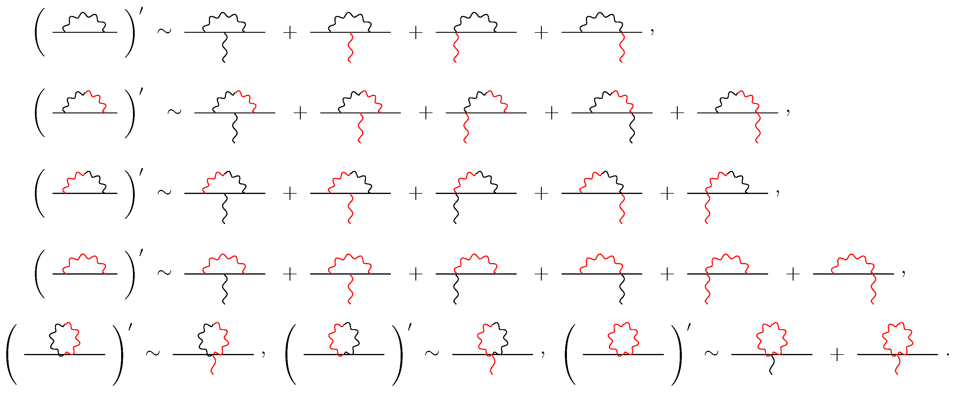
These relations correspond to the diagrams in Figure 12. The derivative of the self-energy diagrams gives rise to the vertex diagrams, generating one external photon field to be attached to the self-energy diagram at all possible places. For example, for the first rainbow self-energy diagram in Figure 12, a photon from minimal substitution or from the gauge link can be attached to the internal lepton line, while only a photon generated from the gauge link can be attached to the vertex. For the fourth rainbow diagram, both minimal substitution and gauge link photons can be attached to the vertex.

The dressed fermion propagator $S\left(p\right)$ can be written in terms of the free fermion propagator and the self-energy as $S\left(p\right)=S_0\left(p\right)+S_0\left(p\right)\mathrm{\Sigma }\left(p\right)S_0\left(p\right)+S_0\left(p\right)\mathrm{\Sigma }\left(p\right)S_0\left(p\right)\mathrm{\Sigma }\left(p\right)S_0\left(p\right)+\cdots$. It is then straightforward to obtain

$$\underset{q\to 0}{lim}S(p+q)\left[-i{\mathrm{\Gamma }}^{\mu }(p+q,p)\right]S\left(p\right)=-{\displaystyle \frac{dS\left(p\right)}{d{p}_{\mu }}},$$

(99)

which corresponds to the Ward–Green–Takahashi identity,

$$\underset{q\to 0}{lim}\left[-i{q}_{\mu }{\mathrm{\Gamma }}^{\mu }(p+q,p)\right]=\underset{q\to 0}{lim}\left[S^{-1}(p+q)-S^{-1}\left(p\right)\right].$$

(100)

The dressed propagator can also be written as

$$S\left(p\right)={\displaystyle \frac{i{Z}_2}{\cancel{p}-m}},$$

(101)

where $Z_2$ is the wave function renormalization constant, and $Z_2-1=d\mathrm{\Sigma }\left(p\right)/d\cancel{p}{|}_{p^2=m^2}$. The Ward–Green–Takahashi identity (100) also implies that

$$Z_2{\mathrm{\Gamma }}^{\mu }(p,p)={\gamma }^{\mu }.$$

(102)

As usual, the Dirac and Pauli form factors are defined as [206]

$$Z_2{\mathrm{\Gamma }}^{\mu }(p+q,p)={\gamma }^{\mu }{F}_1\left(q^2\right)+{\displaystyle \frac{i{\sigma }^{\mu \nu }{q}_{\nu }}{2m}}{F}_2\left(q^2\right),$$

(103)

with normalization $F_1\left(0\right)=1$. This is consistent with the renormalized lepton charge being unity. In the next section, we will use nonlocal QED to calculate the lepton magnetic moments to explore the $g-2$ anomaly.

3.4. $g-2$ Anamaly

The current theoretical prediction for the muon anomalous magnetic moment $a_{\mu }$ in the SM is $a_{\mu }^{\mathrm{SM}}=116,591,810\left(43\right)\times {10}^{-11}$ [125]. The recent measurement of $a_{\mu }$ in the E989 experiment at Fermilab (FNAL) found

$$\mathrm{\Delta }{a}_{\mu }^{\mathrm{FNAL}}\equiv a_{\mu }^{\mathrm{FNAL}}-a_{\mu }^{\mathrm{SM}}=(230\pm 69)\times {10}^{-11},$$

(104)

which is a $3.3\sigma$ discrepancy from the SM prediction [126]. Combined with the previous E821 measurement at Brookhaven National Laboratory (BNL) [127], the result revealed a $4.2\sigma$ deviation from the SM prediction [126]

$$\mathrm{\Delta }{a}_{\mu }=a_{\mu }^{\mathrm{FNAL}+\mathrm{BNL}}-a_{\mu }^{\mathrm{SM}}=(251\pm 59)\times {10}^{-11}.$$

(105)

For the electron, the theoretical prediction for $a_e$ is $a_e^{\mathrm{SM},\mathrm{B}}=1,159,652,182.032\left(720\right)\times {10}^{-12}$ [128], where the superscript “B” refers to the fine structure constant $\alpha$ being measured at Berkeley with ¹³⁷Cs atoms [129]. The most accurate measurement of $a_e$ was made by the Harvard group, and the discrepancy from the SM was $2.4\sigma$ [130],

$$\mathrm{\Delta }{a}_e^{\mathrm{B}}=a_e^{\exp }-a_e^{\mathrm{SM},\mathrm{B}}=(-87\pm 36)\times {10}^{-14}.$$

(106)

However, a new determination [131] of the fine structure constant $\alpha$, obtained from the measurement at LKB with ⁸⁷Rb, improves the accuracy by a factor of 2.5 compared to the previous best measurement at Berkeley [129]. With the new $\alpha$ value, the SM prediction for the electron magnetic moment is $1.6\sigma$ lower than the experimental data,

$$\mathrm{\Delta }{a}_e^{\mathrm{LKB}}=a_e^{\exp }-a_e^{\mathrm{SM},\mathrm{LKB}}=(48\pm 30)\times {10}^{-14}.$$

(107)

It is interesting to note that the two $\mathrm{\Delta }{a}_e$ discrepancies have similar magnitude but opposite sign, for still unidentified reasons [131]. The small difference between the $\alpha$ values does not affect $\mathrm{\Delta }{a}_{\mu }$ since it is much larger than $\mathrm{\Delta }{a}_e$. As the SM predictions match all other experimental information very well, the deviation in one of the most precisely measured quantities in particle physics provides an enduring hint for new physics.

In this section, we will examine the $g-2$ anomaly within nonlocal QED. By inserting the electromagnetic current into the lepton states with initial and final momenta p and $p^{\prime }$, one can obtain the Dirac and Pauli form factors of the lepton. The corresponding Feynman diagrams are given in Ref. [124]. Using the projection method, or calculating two different traces of $\gamma$ matrices, one finds

$$\begin{array}{ccc}& & F_1\left(q^2\right)=-{\displaystyle \frac{A(4m^2-q^2)-6m^{2}B}{4{(4m^2-q^2)}^2}},\hfill \end{array}$$

(108a)

$$\begin{array}{ccc}& & F_2\left(q^2\right)=m^2{\displaystyle \frac{A(4m^2-q^2)-B(2m^2+q^2)}{q^2{(4m^2-q^2)}^2}},\hfill \end{array}$$

(108b)

where A and B can be calculated from the traces

$$\begin{array}{ccc}& & A=\sum _{\mathrm{spin}}\overline{u}\left(p^{\prime }\right){\mathrm{\Gamma }}_{\mu }u\left(p\right)\overline{u}\left(p\right){\gamma }^{\mu }u\left(p^{\prime }\right)=\mathrm{Tr}\left[{\mathrm{\Gamma }}_{\mu }(\cancel{p}+m){\gamma }^{\mu }({\cancel{p}}^{\prime }+m)\right],\hfill \end{array}$$

(109a)

$$\begin{array}{ccc}& & B=\sum _{\mathrm{spin}}\overline{u}\left(p^{\prime }\right){\mathrm{\Gamma }}_{\mu }u\left(p\right)\overline{u}\left(p\right){\displaystyle \frac{{(p+p^{\prime })}^{\mu }}{m}}u\left(p^{\prime }\right)=\mathrm{Tr}\left[{\mathrm{\Gamma }}_{\mu }(\cancel{p}+m)({\cancel{p}}^{\prime }+m){\displaystyle \frac{{(p+p^{\prime })}^{\mu }}{m}}\right].\hfill \end{array}$$

(109b)

In this review, we focus on the Pauli form factor $F_2$, which is related to the anomalous magnetic moment of the lepton. Compared with the standard QED theory, in the nonlocal case, the one-loop vertices are rather more complicated. In addition to the usual QED diagrams, there are an additional 23 diagrams for the nonlocal theory. For the first rainbow diagram, the vertex ${\mathrm{\Gamma }}_1^{\mu }(p,q)$ is expressed as

$$\begin{array}{cc}\hfill {\mathrm{\Gamma }}_1^{\mu }(p,q)& =-e^2\int {\displaystyle \frac{d^{4}k}{{\left(2\pi \right)}^4}}{V}_1^{\nu }(p^{\prime }-k,k)S_0(p-k+q)V_1^{\mu }(p-k,q)\hfill \\ \hfill & \times S_0(p-k)V_1^{\rho }(p,-k)D_{0\nu \rho }\left(k\right).\hfill \end{array}$$

(110)

The corresponding Pauli form factor for the vertex ${\mathrm{\Gamma }}_1^{\mu }(p,q)$ is given by

$$\begin{array}{cc}\hfill F_{2,1}\left(q^2\right)=& {\displaystyle \frac{-8i{e}^2{m}^2}{q^2{(4m^2-q^2)}^2}}\int {\displaystyle \frac{d^{4}k}{{\left(2\pi \right)}^4}}\left[{\displaystyle \frac{(4m^2+2q^2)({(k·p)}^2+{(k·p^{\prime })}^2)-8(m^2-q^2)k·pk·p^{\prime }}{({(p^{\prime }-k)}^2-m^2)({(p-k)}^2-m^2)k^2}}\right.\hfill \\ \hfill & +\left.{\displaystyle \frac{(q^4-4m^2{q}^2)(k·p+k·p^{\prime }+k^2)}{({(p^{\prime }-k)}^2-m^2)({(p-k)}^2-m^2)k^2}}\right]{\tilde{G}}_2(p^{\prime }-k,k){\tilde{G}}_2(p-k,q){\tilde{G}}_2(p,-k).\hfill \end{array}$$

(111)

When the momentum transfer $q^2=0$, one has

$$F_{2,1}\left(0\right)=i{e}^2\int {\displaystyle \frac{d^{4}k}{{\left(2\pi \right)}^4}}{\displaystyle \frac{(3k^2+2k·p)m^2-3{(k·p)}^2}{2k^2{(k^2-2k·p)}^2{m}^2}}{\tilde{G}}_2(p-k,k){\tilde{G}}_2(p-k,0){\tilde{G}}_2(p,-k).$$

(112)

For all other diagrams, the expressions for ${\mathrm{\Gamma }}_i^{\mu }(p,q)$ are given in the Appendix of Ref. [124].

In the numerical calculations, the photon is treated as a point particle, with no modification to its propagator, and the correlation function $F_4\left(a\right)$ in the free photon Lagrangian is chosen to be a delta function, $\delta \left(a\right)$. For the lepton–photon interaction, the functions $F_i(a,b)(i=2,3)$ are assumed to be factorized as $f\left(a\right)F_i\left(b\right)$ to simplify numerical calculation. According to Equation (46), $f\left(a\right)$ is an a-independent constant, equal to 1, and $\int d^{4}b{F}_i\left(b\right)=1$. As a result, the Fourier transforms of the correlators can be written as

$${\tilde{G}}_i(p,q)={\tilde{F}}_1\left(P\right){\tilde{F}}_i\left(q\right).$$

(113)

For the vertex with two and three photons, the correlators can similarly be factorized as

$$\begin{array}{cc}\hfill {\tilde{G}}_{ij}(p,q_1,q_2)& ={\tilde{F}}_1\left(P\right){\tilde{F}}_i\left(q_1\right){\tilde{F}}_j\left(q_2\right),\hfill \end{array}$$

(114)

$$\begin{array}{cc}\hfill {\tilde{G}}_{ijk}(p,q_1,q_2,q_3)& ={\tilde{F}}_1\left(P\right){\tilde{F}}_i\left(q_1\right){\tilde{F}}_j\left(q_2\right){\tilde{F}}_k\left(q_3\right),\hfill \end{array}$$

(115)

where $i,j,k=2$ or 3. The subscript 2 here represents a photon from the minimal substitution, while the subscript 3 is for a photon from the gauge link. The correlators in the interaction vertex are chosen to be

$${\tilde{F}}_2\left(k\right)={\tilde{F}}_3\left(k\right)={\displaystyle \frac{{\mathrm{\Lambda }}_2^2}{{\mathrm{\Lambda }}_2^2-k^2}}.$$

(116)

These correlators were proposed in earlier work [113,123,124] on nonlocal effective field theory and the “minimal” version of nonlocal QED. Here, the free Lagrangian for the lepton is also nonlocal, which gives rise to a modified lepton propagator. For ${\tilde{F}}_1\left(p\right)$ in the free lepton propagator, one can choose

$${\tilde{F}}_1\left(p\right)={\displaystyle \frac{{\mathrm{\Lambda }}_1^2-p^2}{{\mathrm{\Lambda }}_1^2}}.$$

(117)

Since the correlator is in the denominator of Equation (49), the modified propagator makes the loop integration more convergent.

In the above correlators, the cutoff parameters ${\mathrm{\Lambda }}_1$ and ${\mathrm{\Lambda }}_2$ can be determined from $\mathrm{\Delta }{a}_e$ and $\mathrm{\Delta }{a}_{\mu }$, which will give a nonzero difference between the nonlocal QED and SM $\mathrm{\Delta }{a}_l^{\mathrm{nl}}$ results. Note that nonlocal QED itself does not determine the form of the correlation functions or the cutoff parameters, which instead reflect the properties of the particles and need to be determined empirically. In this case, ${\mathrm{\Lambda }}_{2e}$ and ${\mathrm{\Lambda }}_{2\mu }$ are determined for a given ${\mathrm{\Lambda }}_1$ using the experimental $\mathrm{\Delta }{a}_e$ and $\mathrm{\Delta }{a}_{\mu }$ for the chosen correlators.

When ${\mathrm{\Lambda }}_1$ and ${\mathrm{\Lambda }}_2$ are both infinite, nonlocal QED reverts back to the standard local QED. To render the nonlocal effects negligible in other electromagnetic processes, such as Compton scattering, electron–electron scattering, or electron–positron annihilation, large values ($\gtrsim 1$ TeV) are required for the cutoffs. At each vertex, the correlator ${\tilde{F}}_1\left(k\right)$ makes the loop integral more divergent, while ${\tilde{F}}_2\left(k\right)$ and ${\tilde{F}}_3\left(k\right)$ make the integral more convergent. For a given ${\mathrm{\Lambda }}_1$, the smaller the ${\mathrm{\Lambda }}_2$, the smaller the magnetic moment. A lower limit will therefore exist for the magnetic moment for the smallest ${\mathrm{\Lambda }}_2$ value, and if $\mathrm{\Delta }{a}_l$ is below the lower-limit value, it cannot be explained in nonlocal QED for reasonable cutoffs.

In contrast, for a given ${\mathrm{\Lambda }}_2$, the smaller the ${\mathrm{\Lambda }}_1$, the larger the magnetic moment. Since for any ${\mathrm{\Lambda }}_1$, the magnetic moment of the lepton is infinite when ${\mathrm{\Lambda }}_2\to \infty$, there will be no upper limit value for the lepton magnetic moment. For large cutoffs, depending on the specific values of ${\mathrm{\Lambda }}_1$ and ${\mathrm{\Lambda }}_2$, one can obtain lepton magnetic moments larger or smaller relative to the SM results. Since ${\mathrm{\Lambda }}_1$ and ${\mathrm{\Lambda }}_2$ should be process-independent, if the $\mathrm{\Lambda }$ values determined in one process cannot reproduce experimental results in other processes, nonlocal QED would need to be modified further.

In Figure 13, the values of ${\mathrm{\Lambda }}_2$ are plotted versus ${\mathrm{\Lambda }}_1$ for the muon $\mathrm{\Delta }{a}_{\mu }$, electron $\mathrm{\Delta }{a}_e^{\mathrm{LKB}}$, and electron $\mathrm{\Delta }{a}_e^{\mathrm{B}}$ discrepancies. For a given ${\mathrm{\Lambda }}_1$, one can always find a corresponding ${\mathrm{\Lambda }}_2$ to obtain the experimental discrepancies. For the muon, when ${\mathrm{\Lambda }}_1$ is small ($\lesssim 0.8$ TeV), ${\mathrm{\Lambda }}_2$ increases smoothly with increasing ${\mathrm{\Lambda }}_1$, while ${\mathrm{\Lambda }}_2$ increases rapidly when ${\mathrm{\Lambda }}_1\gtrsim 0.8$ TeV. For ${\mathrm{\Lambda }}_1=(0.8,0.9,1.0)$ TeV, for example, one has the corresponding values ${\mathrm{\Lambda }}_2=(0.84,60.23,5.82\times {10}^4$) TeV, respectively. For the electron case, the results for the two discrepancies $\mathrm{\Delta }{a}_e^{\mathrm{LKB}}$ and $\mathrm{\Delta }{a}_e^{\mathrm{B}}$ are quite different. For the negative $\mathrm{\Delta }{a}_e^{\mathrm{B}}$, the obtained ${\mathrm{\Lambda }}_2^{\mathrm{B}}$ is not sensitive to ${\mathrm{\Lambda }}_1$, and for a broad range of ${\mathrm{\Lambda }}_1$ one finds ${\mathrm{\Lambda }}_2^{\mathrm{B}}\approx 10$–20 GeV, which is unreasonably small. The experimental $e^{+}{e}^{-}\to {\mu }^{+}{\mu }^{-}$ cross section, for example, will not be described for small cutoff parameters ${\mathrm{\Lambda }}_2$. However, for the positive $\mathrm{\Delta }{a}_e^{\mathrm{LKB}}$ result, when ${\mathrm{\Lambda }}_1\approx 0.35$ TeV, one obtains ${\mathrm{\Lambda }}_2^{\mathrm{LKB}}\approx 0.55$ TeV. The corresponding ${\mathrm{\Lambda }}_2^{\mathrm{LKB}}$ increases rapidly with increasing ${\mathrm{\Lambda }}_1$ when ${\mathrm{\Lambda }}_1\gtrsim 0.35$ TeV. Since for any ${\mathrm{\Lambda }}_1$ the anomalous magnetic moment of the electron is infinite when ${\mathrm{\Lambda }}_2\to \infty$, one can always find a value of ${\mathrm{\Lambda }}_2^{\mathrm{LKB}}$ to obtain the correct $\mathrm{\Delta }{a}_e^{\mathrm{LKB}}$ for any large ${\mathrm{\Lambda }}_1$.

The muon $g-2$ discrepancy can therefore be well explained with large $\mathrm{\Lambda }$ values, without contradicting other experimental measurements. For the electron, however, $\mathrm{\Delta }{a}_e^{\mathrm{B}}$ cannot be reasonably reproduced in nonlocal QED. As discussed, the correlators ${\tilde{F}}_1\left(k\right)$ and ${\tilde{F}}_{2,3}\left(k\right)$ in the vertex have opposite effects. With an appropriate choice of cutoffs, one can still find negative $\mathrm{\Delta }{a}_e^{\mathrm{nl}}$ with large $\mathrm{\Lambda }$ values, although its absolute value is much smaller than $\mathrm{\Delta }{a}_e^{\mathrm{B}}$. For example, the calculated $\mathrm{\Delta }{a}_e^{\mathrm{nl}}$ is $-4.04\times {10}^{-16}$ with ${\mathrm{\Lambda }}_2=1.0$ TeV and infinite ${\mathrm{\Lambda }}_1$. Certainly, for a given ${\mathrm{\Lambda }}_1$, if ${\mathrm{\Lambda }}_2$ is between ${\mathrm{\Lambda }}_2^{\mathrm{B}}$ and ${\mathrm{\Lambda }}_2^{\mathrm{LKB}}$, the calculated $\mathrm{\Delta }{a}_e^{\mathrm{nl}}$ will lie between $\mathrm{\Delta }{a}_e^{\mathrm{B}}$ and $\mathrm{\Delta }{a}_e^{\mathrm{LKB}}$. For ${\mathrm{\Lambda }}_1=1.0$ TeV, if we assume ${\mathrm{\Lambda }}_2$ for the electron is the same as for the muon, the discrepancy is $\mathrm{\Delta }{a}_e^{\mathrm{nl}}=8.19\times {10}^{-14}$.

Note that nonlocal QED itself does not predict the cutoffs $\mathrm{\Lambda }$, which are determined from the experimental $g-2$ discrepancy. For the electron case, there is a strong sensitivity of ${\mathrm{\Lambda }}_2^{\mathrm{LKB}}$ to ${\mathrm{\Lambda }}_1$, which implies that ${\mathrm{\Lambda }}_2^{\mathrm{LKB}}$ could be very large in order to reconcile the LBK measurement. However, for the Berkeley experimental value, ${\mathrm{\Lambda }}_2^{\mathrm{B}}$ has little sensitivity to ${\mathrm{\Lambda }}_1$, leading to rather small ${\mathrm{\Lambda }}_2^{\mathrm{B}}$ values. Future experimental data may provide further constraints on ${\mathrm{\Lambda }}_2$. If the value lies between the Berkeley and LKB results, the curve for ${\mathrm{\Lambda }}_2$ versus ${\mathrm{\Lambda }}_1$ for the electron will lie between the dashed and dotted lines in Figure 13. Most proposed theoretical solutions to the discrepancy have involved the introduction of new particles, symmetries, and interactions beyond the standard model. While the nonlocal QED framework also requires parameters, the nonlocal extension of local QED is an important alternative to explore given that the lepton $g-2$ discrepancy can be explained without the introduction of new postulated particles beyond the standard model.

We should stress that the SM prediction $a_{\mu }^{\mathrm{SM}}$ has been derived using the leading hadronic vacuum polarization (HVP) contribution to the muon $g-2$, ${\left(a_{\mu }^{\mathrm{HVP}}\right)}_{e^{+}{e}^{-}}^{\mathrm{TI}}=6931\left(40\right)\times {10}^{-11}$, based on low-energy cross section data for $e^{+}{e}^{-}\to$ hadrons obtained by the Muon $g-2$ Theory Initiative [125,207]. Recently, the BMW lattice QCD collaboration [208] also computed the leading HVP contribution to the muon $g-2$. With careful treatments of critical issues such as scale determination, noise reduction, QED, and strong-isospin breaking, as well as infinite-volume and continuum extrapolations, the obtained HVP contribution was found to be ${\left(a_{\mu }^{\mathrm{HVP}}\right)}_{\mathrm{BMW}}=7075\left(55\right)\times {10}^{-11}$. With the larger contribution of ${\left(a_{\mu }^{\mathrm{HVP}}\right)}_{\mathrm{BMW}}$, the discrepancy from the experimental result $\mathrm{\Delta }{a}_{\mu }$ is reduced to 1.6$\sigma$. Obviously, the findings need to be confirmed by other groups using other discretizations of QCD, which are currently underway. With an appropriate choice of the cutoff parameters in the correlation functions, the $1.6\sigma$ discrepancy of the moun $g-2$ can also be obtained in nonlocal QED. For example, for ${\mathrm{\Lambda }}_1=(1.0,1.2,1.4)$ TeV, this can be achieved with ${\mathrm{\Lambda }}_2=(0.23,0.68,71.95)$ TeV, respectively, using the value of the lattice result ${\left(a_{\mu }^{\mathrm{HVP}}\right)}_{\mathrm{BMW}}$ rather than ${\left(a_{\mu }^{\mathrm{HVP}}\right)}_{e^{+}{e}^{-}}^{\mathrm{TI}}$.

To illustrate the lepton mass dependence of the calculated lepton anomalous magnetic moment discrepancy, in Figure 14, we show $\mathrm{\Delta }{a}_l^{\mathrm{nl}}$ versus the lepton mass, $m_l$, for ${\mathrm{\Lambda }}_1=1$ TeV. Since ${\mathrm{\Lambda }}_2$ for the electron is not well determined because of the two different experimental results, for any mass $m_l$, ${\mathrm{\Lambda }}_2$ is chosen to agree with the experimental $\mathrm{\Delta }{a}_{\mu }$ value for ${\mathrm{\Lambda }}_1=1$ TeV. For $m_l=m_{\mu }$, the discrepancy $\mathrm{\Delta }{a}_l^{\mathrm{nl}}$ coincides with the experimental discrepancy $\mathrm{\Delta }{a}_{\mu }$. For $m_l=m_e$, the calculated $\mathrm{\Delta }{a}_l^{\mathrm{nl}}$ is larger than $\mathrm{\Delta }{a}_e^{\mathrm{B}}$, but smaller than $\mathrm{\Delta }{a}_e^{\mathrm{LKB}}$. The discrepancy $\mathrm{\Delta }{a}_l^{\mathrm{nl}}$ increases with increasing lepton mass, and it is $5.62\times {10}^{-7}$ when $m_l$ is at the mass of the $\tau$ lepton, which is obviously covered by the large experimental uncertainty ($-0.040$, 0.019) [209]. With nonlocal QED, both the muon and electron $g-2$ anomalies can therefore be reasonably well explained. In contrast to other theoretical methods, this calculation does not require the introduction of any new symmetries or new particles. The large positive discrepancy $\mathrm{\Delta }{a}_{\tau }^{\mathrm{nl}}$ for $\tau$ leptons can be tested by precise experiments in the future.

4. Gravitational Form Factors

While electromagnetic probes have been the primary tool used to study the structure of hadrons, characterizing the gravitational properties of hadrons can also reveal fundamental information about their internal structure. In the final example of a nonlocal field theory, we discuss its application to the calculation of the gravitational form factors, beginning first with a review of some basic elements of nonlocal gravity and the energy–momentum tensor. In contrast to the previous sections, here, we present a novel application of nonlocal theory in a curved spacetime.

4.1. Nonlocal Gravity

We begin by introducing the nonlocal actions for pion–nucleon interactions in curved spacetime. Theoretically, the action in curved spacetime can be constructed by modifying the covariant derivatives and introducing the metric tensor $g^{\mu \nu }$ and vierbein fields $e_a^{\mu }$. To illustrate the gauge-field-like nature of gravity, we firstly review the “gauge” transformation properties of the nucleon, pion, and gravitational fields. Under a general coordinate transformation, these transform according to [210,211,212]

$$\begin{array}{ccc}\hfill x^{\mu }& \to & x^{\mu }+\kappa {\xi }^{\mu }\left(x\right),\hfill \end{array}$$

(118a)

$$\begin{array}{ccc}\hfill \varphi \left(x\right)& \to & \varphi \left(x\right),\hfill \end{array}$$

(118b)

$$\begin{array}{ccc}\hfill g^{\mu \nu }\left(x\right)& \to & g^{\mu \nu }\left(x\right)+\kappa [{\partial }^{\mu }{\xi }^{\nu }\left(x\right)+{\partial }^{\nu }{\xi }^{\mu }\left(x\right)],\hfill \end{array}$$

(118c)

$$\begin{array}{ccc}\hfill e_a^{\mu }\left(x\right)& \to & e_a^{\mu }\left(x\right)+\kappa {\partial }_a{\xi }^{\mu }\left(x\right),\hfill \end{array}$$

(118d)

$$\begin{array}{ccc}\hfill {\partial }_{\mu }& \to & {\partial }_{\mu }-\kappa {\partial }_{\mu }{\xi }^{\alpha }\left(x\right){\partial }_{\alpha },\hfill \end{array}$$

(118e)

where ${\kappa }^2=32\pi G$ represents the gravitational coupling constant, $\varphi$ denotes the pion field, taking the form $\varphi =({\pi }^{+},{\pi }^{-},{\pi }^0)$ and ${\xi }^{\mu }\left(x\right)$ is a infinitesimal vector parameter. Note that the gravitational metric field $g^{\mu \nu }$ and the vierbein field $e_{\mu }^a$ include both flat Minkowski and curved spacetime backgrounds. In order to manifestly illustrate the feature of curved spacetime, it is necessary to separate the two backgrounds from each other. This can be done in the weak gravitational background limit, where the metric $g^{\mu \nu }$, vierbein $e_a^{\mu }$, and $\sqrt{-g}$ fields (where $g\equiv det\left(g_{\mu \nu }\right)$) can be expanded around the flat spacetime as [212,213,214]

$$\begin{array}{ccc}\hfill g_{\mu \nu }& \equiv & {\eta }_{\mu \nu }+\kappa h_{\mu \nu },\hfill \end{array}$$

(119a)

$$\begin{array}{ccc}\hfill g^{\mu \nu }& =& {\eta }^{\mu \nu }-\kappa h^{\mu \nu }+\mathcal{O}\left({\kappa }^2\right),\hfill \end{array}$$

(119b)

$$\begin{array}{ccc}\hfill \sqrt{-g}& =& 1+{\displaystyle \frac{1}{2}}\kappa h+\mathcal{O}\left({\kappa }^2\right),\hfill \end{array}$$

(119c)

$$\begin{array}{ccc}\hfill e_a^{\mu }& =& {\delta }_a^{\mu }-{\displaystyle \frac{\kappa }{2}}{\eta }_{a\lambda }{h}^{\lambda \mu }+\mathcal{O}\left({\kappa }^2\right),\hfill \end{array}$$

(119d)

$$\begin{array}{ccc}\hfill e_{\mu }^a& =& {\delta }_{\mu }^a+{\displaystyle \frac{\kappa }{2}}{\eta }^{a\lambda }{h}_{\lambda \mu }+\mathcal{O}\left({\kappa }^2\right),\hfill \end{array}$$

(119e)

where ${\eta }_{\mu \nu }$ is the Minkowski metric $diag(1,-1,-1,-1)$, ${\delta }_a^{\mu }$ the vierbein in flat spacetime, $h_{\mu \nu }$ the gravitational field, and $h={\eta }_{\mu \nu }{h}^{\mu \nu }$. With Equations (119), the Riemann curvature tensor, Ricci tensor, scalar curvature, Christoffel symbol, and spin connection of a Dirac fermion can then be written as [212,213]

$$\begin{array}{ccc}\hfill R_{\sigma \mu \nu }^{\rho }& =& {\partial }_{\mu }{\mathrm{\Gamma }}_{\sigma \nu }^{\rho }-{\partial }_{\nu }{\mathrm{\Gamma }}_{\sigma \mu }^{\rho }+{\mathrm{\Gamma }}_{\mu \lambda }^{\rho }{\mathrm{\Gamma }}_{\sigma \nu }^{\lambda }-{\mathrm{\Gamma }}_{\nu \lambda }^{\rho }{\mathrm{\Gamma }}_{\sigma \mu }^{\lambda }\hfill \end{array}$$

(120a)

$$\begin{array}{ccc}\hfill R_{\mu \nu }& =& R_{\mu \rho \nu }^{\rho }={\displaystyle \frac{\kappa }{2}}[{\partial }_{\mu }{\partial }^{\lambda }{h}_{\lambda \nu }+{\partial }_{\nu }{\partial }^{\lambda }{h}_{\lambda \mu }-{\partial }_{\mu }{\partial }_{\nu }h-{\partial }^2{h}_{\mu \nu }]+\mathcal{O}\left({\kappa }^2\right),\hfill \end{array}$$

(120b)

$$\begin{array}{ccc}\hfill R& =& g^{\mu \nu }{R}_{\mu \nu }=\kappa [{\partial }^{\mu }{\partial }^{\nu }{h}_{\mu \nu }-{\partial }^{2}h]+\mathcal{O}\left({\kappa }^2\right),\hfill \end{array}$$

(120c)

$$\begin{array}{ccc}\hfill {\mathrm{\Gamma }}_{\alpha \beta }^{\lambda }& =& {\displaystyle \frac{\kappa }{2}}{\eta }^{\lambda \sigma }\left({\partial }_{\alpha }{h}_{\beta \sigma }+{\partial }_{\beta }{h}_{\alpha \sigma }-{\partial }_{\sigma }{h}_{\alpha \beta }\right)+\mathcal{O}\left({\kappa }^2\right),\hfill \end{array}$$

(120d)

$$\begin{array}{ccc}\hfill {\omega }_{\mu }^{ab}& =& {\displaystyle \frac{\kappa }{2}}({\partial }^b{h}_{\mu }^a-{\partial }^a{h}_{\mu }^b)+\mathcal{O}\left({\kappa }^2\right),\hfill \end{array}$$

(120e)

respectively.

Physically, nonlocal interactions involving hadrons can be considered to be more realistic than local interactions, given the non-pointlike nature of physical hadrons. This feature can be taken into account by defining a nucleon field at a spacetime point $x_{\mu }$ and displacing the meson or gauge field by a distance $a_{\mu }$ to spacetime point $x_{\mu }+a_{\mu }$ with a correlation function $F\left(a\right)$. To guarantee local gauge invariance, the Wilson line operator needs to be introduced. For the electromagnetic case, one has

$${\mathcal{G}}_{\varphi }^q(x,y)=exp\left[-i{e}_{\varphi }^q{\int }_x^{y}d{z}^{\mu }\int d^{4}lF\left(l\right)A_{\mu }(z+l)\right],$$

(121)

where $A^{\mu }\left(x\right)$ is the photon field. For the gravitational interaction, the local “gauge transformation” could be a local coordinate translation, as in Equation (118), with the corresponding “gauge field” corresponding to the gravitational field. In Refs. [215,216,217], it was argued that the gravitational Wilson line is a double copy of that of the gauge theory. In other words, the gravitational Wilson line operator can be obtained by replacing the gauge field in U(1) gauge link with the gravitational field. By analogy with the U(1) gauge link, the gravitational Wilson line operator can be constructed as [218]

$$\begin{array}{ccc}\hfill W(x,y)& \equiv & exp\left[-{\displaystyle \frac{\kappa }{4}}{\int }_x^y\int d^{4}lF\left(l\right)h^{\mu \nu }(z+l)d{z}_{\{\mu }{\partial }_{\nu \}}\right],\hfill \end{array}$$

(122a)

$$\begin{array}{ccc}\hfill W_{\nu }^{\mu }(x,y)& \equiv & exp\left[{\int }_x^y\int d^{4}lF\left(l\right)\left(-{\displaystyle \frac{\kappa }{4}}{\delta }_{\nu }^{\mu }{h}^{\alpha \beta }(z+l)d{z}_{\{\alpha }{\partial }_{\beta \}}-{\mathrm{\Gamma }}_{\rho \nu }^{\mu }(z+l)d{z}^{\rho }\right)\right],\hfill \end{array}$$

(122b)

where $F\left(l\right)$ is the correlation function for the nonlocal interaction. The tensor $h^{\mu \nu }$ represents the gravitational field and transforms as $h^{\mu \nu }\to h^{\mu \nu }+\kappa \left[{\partial }^{\mu }{\xi }^{\prime \nu }+{\partial }^{\nu }{\xi }^{\prime \mu }\right]$. Note that, here, the infinitesimal parameters ${\xi }^{\prime \mu }$ for the gravitational field are different from ${\xi }^{\mu }$ for matter fields, which is similar to the local U(1) transformation. In the nonlocal framework, the pion kinetic term in curved spacetime can be written as [78,218]

$$S_{\varphi {\varphi }^{†}}^{\left(2\right),\mathrm{nl}}=\int d^{4}x\int d^{4}lF\left(l\right)\sqrt{-g(x+l)}\left[{\displaystyle \frac{g^{\mu \nu }(x+l)}{2}}{\partial }_{\{\mu }\varphi \left(x\right){\partial }_{\nu \}}{\varphi }^{†}\left(x\right)-m_{\varphi }^2\varphi \left(x\right){\varphi }^{†}\left(x\right)\right],$$

(123)

where $m_{\varphi }$ is the pion mass and we assume the correlation function satisfies $\int d^{4}lF\left(l\right)=1$. The mesonic action (123) is invariant under the coordinate transformations of Equation (118) if ${\xi }^{\prime \mu }$ and ${\xi }^{\mu }$ are related by $\int d^{4}lF\left(l\right){\xi }^{\prime \mu }(x+l)={\xi }^{\mu }\left(x\right)$. The leading-order pion–nucleon action in curved spacetime can be constructed as [78,218]

$$\begin{array}{cc}\hfill S_{\varphi N}^{\left(1\right),\mathrm{nl}}& =\int d^{4}x\int d^{4}lF\left(l\right)\sqrt{-g(x+l)}\{{\displaystyle \frac{i}{2}}\overline{N}\left(x\right)e_a^{\mu }(x+l){\gamma }^a{\nabla }_{\mu }N\left(x\right)\hfill \\ \hfill & -{\displaystyle \frac{i}{2}}{\nabla }_{\mu }\overline{N}\left(x\right)e_a^{\mu }(x+l){\gamma }^{a}N\left(x\right)-M\overline{N}\left(x\right)N\left(x\right)\hfill \\ \hfill & +{\delta }_2\left[{\displaystyle \frac{i}{2}}\overline{N}\left(x\right)e_a^{\mu }\left(x\right){\gamma }^a{\nabla }_{\mu }N\left(x\right)-{\displaystyle \frac{i}{2}}{\nabla }_{\mu }\overline{N}\left(x\right)e_a^{\mu }\left(x\right){\gamma }^{a}N\left(x\right)\right]-{\delta }_M\overline{N}\left(x\right)N\left(x\right)\}\hfill \\ \hfill & -{\displaystyle \frac{C_{N\varphi }}{f_{\varphi }}}\int d^{4}x\int d^{4}a\int d^{4}lF\left(a\right)F\left(l\right)\hfill \\ \hfill & \times \sqrt{-g(x+l)}\overline{p}\left(x\right){\gamma }^a{\gamma }^5{e}_a^{\mu }(x+l)B\left(x\right)W_{\mu }^{\nu }(x,x+a)D_{\nu }\varphi (x+a)+\mathrm{H}.\mathrm{c}.\hfill \\ \hfill & -i{\displaystyle \frac{C_{\varphi {\varphi }^{†}}}{2f_{\varphi }^2}}\int d^{4}x\int d^{4}a\int d^{4}b\int d^{4}lF\left(a\right)F\left(b\right)F\left(l\right)\sqrt{-g(x+l)}\overline{p}\left(x\right){\gamma }^a{e}_a^{\mu }\left(x_l\right)p\left(x\right)\hfill \\ \hfill & \times \{\left[W_{\mu }^{\nu }(x,x+a)D_{\nu }\varphi (x+a)\right]{\left[W(x,x+b)\varphi (x+b)\right]}^{†}\hfill \\ \hfill & -\left[W(x,x+b)\varphi \left(x_b\right)\right]{\left[W_{\mu }^{\nu }(x,x_a)D_{\nu }\varphi (x+a)\right]}^{†}\},\hfill \end{array}$$

(124)

where $N\left(x\right)={[p\left(x\right),n\left(x\right)]}^T$ denotes the intermediate nucleon (proton $p\left(x\right)$ or neutron $n\left(x\right)$) field, and M is the physical mass of the nucleon. The constants $C_{N\varphi }$ and $C_{\varphi {\varphi }^{†}}$ represent the leading-order pion–nucleon coupling constants for different channels, as listed in

Table 2. Effective pion–nucleon coupling constants (for proton external states) $C_{N\varphi }$ and $C_{\varphi {\varphi }^{†}}$ for the leading-order $pN\varphi$ and $pp\varphi \varphi$ interactions, respectively, and $C_{\varphi {\varphi }^{†}}^{\left(1\right)}$, $C_{\varphi {\varphi }^{†}}^{\left(2\right)}$ and $C_{\varphi {\varphi }^{†}}^{\left(3\right)}$ for the next-to-leading order $pp\varphi \varphi$ interactions.

${\mathit{C}}_{\mathit{N}\mathit{\varphi }}$		${\mathit{C}}_{\mathit{\varphi }{\mathit{\varphi }}^{†}}$	${\mathit{C}}_{\mathit{\varphi }{\mathit{\varphi }}^{†}}^{\left(1\right)}$		${\mathit{C}}_{\mathit{\varphi }{\mathit{\varphi }}^{†}}^{\left(2\right)}$		${\mathit{C}}_{\mathit{\varphi }{\mathit{\varphi }}^{†}}^{\left(3\right)}$
$\left(p{\pi }^0\right)$	$\left(n{\pi }^{+}\right)$	$\left({\pi }^{+}{\pi }^{-}\right)$	$\left({\pi }^{+}{\pi }^{-}\right)$	$\left({\pi }^0{\pi }^0\right)$	$\left({\pi }^{+}{\pi }^{-}\right)$	$\left({\pi }^0{\pi }^0\right)$	$\left({\pi }^{+}{\pi }^{-}\right)$	$\left({\pi }^0{\pi }^0\right)$
${\displaystyle \frac{1}{2}}{g}_A$	${\displaystyle \frac{1}{\sqrt{2}}}{g}_A$	${\displaystyle \frac{1}{2}}$	$-4$	$-2$	$-{\displaystyle \frac{1}{2}}$	$-{\displaystyle \frac{1}{4}}$	2	1

. Additionally, ${\delta }_2$ and ${\delta }_M$ are the mass and wave function renormalization counterterm coefficients, related to the wave function renormalization constant $Z_2$ and bare nucleon mass $M_0$ via ${\delta }_2=Z_2-1$ and ${\delta }_M=Z_2{M}_0-M$. The gravitational gauge link operators $W(x,x+a)\varphi (x+a)$ and $W_{\nu }^{\mu }(x,x+a){\partial }_{\mu }\varphi (x+a)$ can be expanded in powers of the gravitational field $h_{\alpha \beta }\left(x\right)$ as

$$\begin{array}{ccc}\hfill W(x,x+a)\varphi (x+a)& =& \varphi (x+a)\hfill \\ & & -{\displaystyle \frac{\kappa }{4}}\int d^{4}l{\int }_x^{x+a}F\left(l\right)h^{\alpha \beta }(z+l)d{z}_{\{\alpha }{\partial }_{\beta \}}\varphi (x+a)+\mathcal{O}\left({\kappa }^2\right),\hfill \end{array}$$

(125a)

$$\begin{array}{ccc}\hfill W_{\nu }^{\mu }(x,x+a){\partial }_{\mu }\varphi (x+a)& =& {\partial }_{\nu }\varphi (x+a)+\int d^{4}l{\int }_x^{x+a}F\left(l\right)\hfill \\ \hfill \times (-{\displaystyle \frac{\kappa }{4}}{\delta }_{\nu }^{\lambda }{h}^{\alpha \beta }(z& + & l)d{z}_{\{\alpha }{\partial }_{\beta \}}-{\mathrm{\Gamma }}_{\mu \nu }^{\lambda }(z+l)d{z}^{\mu }){\partial }_{\lambda }\varphi (x+a)+\mathcal{O}\left({\kappa }^2\right).\hfill \end{array}$$

(125b)

Note that the last two terms of Equation (125b) yield an additional gauge link vertex, which is crucial for gauge invariance of the total energy–momentum tensor in the nonlocal case. These terms vanish in the local limit, $F\left(a\right)\to {\delta }^4\left(a\right)$, and the nonlocal action (124) reduces to the local one. In a similar manner, the nonlocal action for the next-to-leading order pion–nucleon interaction in curved spacetime is constructed as [78,218]

$$\begin{array}{cc}\hfill S_{\varphi N}^{\left(2\right),\mathrm{nl}}=& 4c_1{m}_{\varphi }^2\int d^{4}x\int d^{4}lF\left(l\right)\sqrt{-g(x+l)}\overline{p}\left(x\right)p\left(x\right)\hfill \\ \hfill & +c_1{\displaystyle \frac{m_{\varphi }^2{C}_{\varphi {\varphi }^{†}}^{\left(1\right)}}{f_{\varphi }^2}}\int d^{4}x\int d^{4}a\int d^{4}b\int d^{4}lF\left(a\right)F\left(b\right)F\left(l\right)\sqrt{-g(x+l)}\overline{p}\left(x\right)p\left(x\right)\hfill \\ \hfill & \times \left[W(x,x+a)\varphi (x+a)\right]{\left[W(x,x+b)\varphi (x+b)\right]}^{†}\hfill \\ \hfill & +c_2{\displaystyle \frac{C_{\varphi {\varphi }^{†}}^{\left(2\right)}}{M^2{f}_{\varphi }^2}}\int d^{4}x\int d^{4}a\int d^{4}b\int d^{4}lF\left(a\right)F\left(b\right)F\left(l\right)\sqrt{-g(x+l)}{g}^{\alpha \mu }(x+l)g^{\beta \nu }(x+l)\hfill \\ \hfill & \times \left(\overline{p}\left(x\right){\nabla }_{\alpha }{\nabla }_{\beta }p\left(x\right)+{\nabla }_{\alpha }{\nabla }_{\beta }\overline{p}\left(x\right)p\left(x\right)\right)\hfill \\ \hfill & \times \left[W_{\{\mu }^{\rho }(x,x+a)D_{\rho }\varphi (x+a)\right]{\left[W_{\nu \}}^{\lambda }(x,x+b)D_{\lambda }\varphi (x+b)\right]}^{†}\hfill \\ \hfill & +c_3{\displaystyle \frac{C_{\varphi {\varphi }^{†}}^{\left(3\right)}}{2f_{\varphi }^2}}\int d^{4}x\int d^{4}a\int d^{4}b\int d^{4}lF\left(a\right)F\left(b\right)F\left(l\right)\sqrt{-g(x+l)}\overline{p}\left(x\right)g^{\mu \nu }(x+l)p\left(x\right)\hfill \\ \hfill & \times \left[W_{\{\mu }^{\alpha }(x,x+a)D_{\alpha }\varphi (x+a)\right]{\left[W_{\nu \}}^{\beta }(x,x+b)D_{\beta }\varphi (x+b)\right]}^{†},\hfill \end{array}$$

(126)

where $C_{\varphi {\varphi }^{†}}^{\left(1\right)}$, $C_{\varphi {\varphi }^{†}}^{\left(2\right)}$, and $C_{\varphi {\varphi }^{†}}^{\left(3\right)}$ are the pion–nucleon coupling constants at next-to-leading order for different channels, listed in Table 2. Finally, the nonlocal version of nonminimal coupling between the nucleon and the gravitational field can be written as [78,218]

$$\begin{array}{ccc}\hfill S_{\mathrm{nonmin}}^{\mathrm{nl}}& =& \int d^{4}x\int d^{4}lF\left(l\right)\sqrt{-g(x+l)}\{{\displaystyle \frac{c_8}{8}}R(x+l)\overline{N}\left(x\right)N\left(x\right)\hfill \\ & & +i{\displaystyle \frac{c_9}{M}}{R}^{\mu \nu }(x+l)\left[\overline{N}\left(x\right)e_{\mu }^a(x+l){\gamma }_a{\nabla }_{\nu }N\left(x\right)-{\nabla }_{\nu }\overline{N}\left(x\right)e_{\mu }^a(x+l){\gamma }_{a}N\left(x\right)\right]\}.\hfill \end{array}$$

(127)

Expanding the nonlocal actions around the flat spacetime background using Equations (119) and (120), and substituting these into Equations (123), (124), (126) and (127), one can obtain explicit actions for the interaction between the matter field and the gravitational field $h^{\mu \nu }$. For example, the leading-order mesonic action of Equation (123) can be rewritten as

$$\begin{array}{cc}\hfill S_{\varphi {\varphi }^{†}}^{\left(2\right),\mathrm{nl}}& =\int d^{4}x\int d^{4}lF\left(l\right)\{{\partial }_{\mu }\varphi \left(x\right){\partial }^{\mu }{\varphi }^{†}\left(x\right)-m_{\varphi }^2\varphi \left(x\right){\varphi }^{†}\left(x\right)\hfill \\ \hfill & +{\displaystyle \frac{1}{2}}\kappa h(x+l)\left[{\partial }_{\mu }\varphi \left(x\right){\partial }^{\mu }{\varphi }^{†}\left(x\right)-m_{\varphi }^2\varphi \left(x\right){\varphi }^{†}\left(x\right)\right]\hfill \\ \hfill & -{\displaystyle \frac{1}{2}}\kappa h^{\mu \nu }\left(x_l\right){\partial }_{\{\mu }\varphi \left(x\right){\partial }_{\nu \}}{\varphi }^{†}\left(x\right)\}+\mathcal{O}\left({\kappa }^2\right),\hfill \end{array}$$

(128)

where the first two terms represent the pion kinetic action in flat spacetime, and the last three terms represent the lowest-order interaction between the pion and the gravitational field. Similarly, the leading-order pion–nucleon interaction in Equation (124) can be expanded as

$$\begin{array}{ccc}\hfill S_{\varphi N}^{\left(1\right),\mathrm{nl}}& =& \int d^{4}x\int d^{4}lF\left(l\right)\{-(M+{\delta }_M)\left(1+{\displaystyle \frac{1}{2}}\kappa h(x+l)\right)\overline{N}\left(x\right)N\left(x\right)\hfill \\ & & +{\displaystyle \frac{i}{2}}(1+{\delta }_2)\left(1+{\displaystyle \frac{1}{2}}\kappa h(x+l)\right)\left[\overline{N}\left(x\right){\gamma }^{\mu }{\partial }_{\mu }N\left(x\right)-{\partial }^{\mu }\overline{N}\left(x\right){\gamma }_{\mu }N\left(x\right)\right]\hfill \\ & & -{\displaystyle \frac{i}{4}}(1+{\delta }_2)\kappa h^{\mu \nu }(x+l)\left[\overline{N}\left(x\right){\gamma }_{\mu }{\partial }_{\nu }N\left(x\right)-{\partial }_{\mu }\overline{N}\left(x\right){\gamma }_{\nu }N\left(x\right)\right]\}\hfill \\ & -& {\displaystyle \frac{C_{N\varphi }}{f_{\varphi }}}\int d^{4}x\int d^{4}l\int d^{4}aF\left(a\right)F\left(l\right)\overline{p}\left(x\right){\gamma }^{\mu }{\gamma }^{5}N\left(x\right)\{\left(1+{\displaystyle \frac{1}{2}}\kappa h(x+l)\right)\hfill \\ & & \times [{\partial }_{\mu }\varphi (x+a)-{\displaystyle \frac{1}{2}}\kappa h^{\nu \lambda }(x+l){\eta }_{\lambda \mu }{\partial }_{\nu }\varphi (x+a)\hfill \\ & & -{\displaystyle \frac{\kappa }{4}}{\int }_x^{x+a}{h}^{\alpha \beta }(z+l)d{z}_{\{\alpha }{\partial }_{\beta \}}{\partial }_{\mu }\varphi (x+a)\hfill \\ & & -{\int }_x^{x+a}{\mathrm{\Gamma }}_{\beta \mu }^{\alpha }(x+l)d{z}^{\beta }{\partial }_{\alpha }\varphi (x+a)+\mathrm{H}.\mathrm{c}.\left]\right\}\hfill \\ & -& i{\displaystyle \frac{C_{\varphi {\varphi }^{†}}}{2f_{\varphi }^2}}\int d^{4}x\int d^{4}l\int d^{4}a\int d^{4}bF\left(a\right)F\left(b\right)F\left(l\right)\overline{p}\left(x\right){\gamma }^{\mu }p\left(x\right)\hfill \\ & & \times \{\left(1+{\displaystyle \frac{1}{2}}\kappa h(x+l)\right)\left[{\partial }_{\mu }\varphi (x+a){\varphi }^{†}(x+b)-\varphi (x+b){\partial }_{\mu }{\varphi }^{†}(x+a)\right]\hfill \\ & & -{\displaystyle \frac{1}{2}}\kappa {\eta }_{\mu \lambda }{h}^{\nu \lambda }(x+l)\left[{\partial }_{\nu }\varphi (x+a){\varphi }^{†}(x+b)-\varphi (x+b){\partial }_{\nu }{\varphi }^{†}(x+a)\right]\hfill \\ & & -{\varphi }^{†}(x+a){\int }_x^{x+b}d{z}^{\lambda }{\mathrm{\Gamma }}_{\lambda \mu }^{\alpha }(z+l){\partial }_{\alpha }\varphi (z+b)\hfill \\ & & -{\displaystyle \frac{1}{4}}{\partial }_{\mu }\varphi (x+b){\int }_x^{x+a}d{z}_{\beta }{h}^{\alpha \beta }(x+l){\partial }_{\alpha }{\varphi }^{†}(x+a)\hfill \\ & & -{\displaystyle \frac{1}{4}}{\varphi }^{†}(x+b){\int }_x^{x+a}d{z}_{\beta }{h}^{\alpha \beta }(x+l){\partial }_{\mu }{\partial }_{\alpha }\varphi (x+a)+\mathrm{H}.\mathrm{c}.\}\hfill \\ & +& \mathcal{O}\left({\kappa }^2\right),\hfill \end{array}$$

(129)

where the $\kappa$-independent terms represent the leading-order strong interaction between pion and nucleon in flat spacetime, while terms proportional to $\kappa$ are interactions between the gravitational and matter fields. The terms with the path integral from x to $x+a$ in Equation (129) are from the gravitational Wilson line operator of Equation (125b). Such terms will generate additional energy–momentum tensor vertices in the nonlocal case. Similarly, the weak field expansion of the next-to-leading order action of Equation (126) yields

$$\begin{array}{cc}\hfill S_{\varphi N}^{\left(2\right),\mathrm{nl}}& =4c_1{m}_{\varphi }^2\int d^{4}x\int d^{4}lF\left(l\right)\left(1+{\displaystyle \frac{1}{2}}\kappa h(x+l)\right)\overline{p}\left(x\right)p\left(x\right)\hfill \\ \hfill & +c_1{m}_{\varphi }^2{\displaystyle \frac{C_{\varphi {\varphi }^{†}}^{\left(1\right)}}{f_{\varphi }^2}}\int d^{4}x\int d^{4}l\int d^{4}a\int d^{4}bF\left(a\right)F\left(b\right)F\left(l\right)\overline{p}\left(x\right)p\left(x\right)\hfill \\ \hfill & \times \{\left[1+{\displaystyle \frac{\kappa h(x+l)}{2}}\right]\varphi (x+a){\varphi }^{†}(x+b)\hfill \\ \hfill & -{\displaystyle \frac{\kappa }{4}}\varphi (x+a){\int }_x^{x+b}{h}^{\alpha \beta }(z+l)d{z}_{\{\alpha }{\partial }_{\beta \}}{\varphi }^{†}(x+b)+\mathrm{H}.\mathrm{c}.\}\hfill \\ \hfill & +c_2{\displaystyle \frac{C_{\varphi {\varphi }^{†}}^{\left(2\right)}}{M^2{f}_{\varphi }^2}}\int d^{4}x\int d^{4}l\int d^{4}a\int d^{4}bF\left(a\right)F\left(b\right)F\left(l\right)\{\left[\overline{p}\left(x\right){\partial }^{\alpha }{\partial }^{\beta }p\left(x\right)+{\partial }^{\beta }{\partial }^{\alpha }\overline{p}\left(x\right)p\left(x\right)\right]\hfill \\ \hfill & \times [\left(1+\kappa {\displaystyle \frac{h(x+l)}{2}}\right){\partial }_{\{\alpha }\varphi (x+a){\partial }_{\beta \}}{\varphi }^{†}(x+b)\hfill \\ \hfill & -\kappa h^{\beta \nu }(x+l){\partial }_{\{\nu }\varphi (x+a){\partial }^{\alpha \}}{\varphi }^{†}(x+b)-\kappa h^{\alpha \mu }\left(x_l\right){\partial }^{\{\beta }\varphi (x+a){\partial }_{\mu \}}{\varphi }^{†}(x+b)\hfill \\ \hfill & -{\displaystyle \frac{\kappa }{4}}{\int }_x^{x+a}{h}^{\mu \nu }(z+l)d{z}_{\{\mu }{\partial }_{\nu }\}{\partial }^{\{\alpha }\varphi (x+a){\partial }^{\beta \}}{\varphi }^{†}(x+b)\hfill \\ \hfill & -\kappa {\int }_x^{x+a}{\mathrm{\Gamma }}_{\sigma \{\alpha }^{\lambda }(z+l)d{z}^{\sigma }{\partial }_{\lambda }\varphi (x+a){\partial }_{\beta \}}{\varphi }^{†}(x+b)+\mathrm{H}.\mathrm{c}.]\hfill \\ \hfill & +[-{\displaystyle \frac{\kappa }{2}}\left({\partial }_{\alpha }{h}_{\beta \sigma }+{\partial }_{\beta }{h}_{\alpha \sigma }-{\partial }_{\sigma }{h}_{\alpha \beta }\right)(x+l)\overline{p}\left(x\right){\partial }^{\sigma }p\left(x\right)\hfill \\ \hfill & -{\displaystyle \frac{\kappa }{2}}\left({\partial }_{\alpha }{h}_{\beta \sigma }+{\partial }_{\beta }{h}_{\alpha \sigma }-{\partial }_{\sigma }{h}_{\alpha \beta }\right)(x+l){\partial }^{\sigma }\overline{p}\left(x\right)p\left(x\right)\hfill \\ \hfill & +\kappa \left({\displaystyle \frac{i}{2}}\overline{p}\left(x\right){\partial }^b{h}_{\{\alpha }^a(x+l){\sigma }_{ab}{\partial }_{\beta \}}p\left(x\right)-{\displaystyle \frac{i}{2}}{\partial }_{\{\beta }\overline{p}\left(x\right){\partial }^b{h}_{\alpha \}}^a\left(x_l\right){\sigma }_{ab}p\left(x\right)\right)]\hfill \\ \hfill & \times {\partial }^{\{\alpha }\varphi (x+a){\partial }^{\beta \}}{\varphi }^{†}(x+b)\}\hfill \\ \hfill & +c_3{\displaystyle \frac{C_{\varphi {\varphi }^{†}}^{\left(3\right)}}{2f_{\varphi }^2}}\int d^{4}x\int d^{4}l\int d^{4}a\int d^{4}bF\left(a\right)F\left(b\right)F\left(l\right)\overline{p}\left(x\right)p\left(x\right)\hfill \\ \hfill & \times \{2\left(1+{\displaystyle \frac{\kappa }{2}}h(x+l)\right){\partial }^{\mu }\varphi (x+a){\partial }_{\mu }{\varphi }^{†}(x+b)-\kappa {\partial }_{\{\nu }\varphi (x+a){\partial }_{\mu \}}{\varphi }^{†}(x+b)h^{\mu \nu }(x+l)\hfill \\ \hfill & -{\displaystyle \frac{\kappa }{2}}{\partial }^{\mu }\varphi (x+a){\int }_x^{x+b}{h}^{\alpha \beta }(z+l)d{z}_{\{\alpha }{\partial }_{\beta \}}{\partial }_{\mu }{\varphi }^{†}(x+b)\hfill \\ \hfill & -2{\partial }^{\mu }\varphi (x+a){\int }_x^{x+b}{\mathrm{\Gamma }}_{\beta \mu }^{\alpha }(z+l)d{z}^{\beta }{\partial }_{\alpha }{\varphi }^{†}(x+b)+\mathrm{H}.\mathrm{c}.\}\hfill \\ \hfill & +\mathcal{O}\left({\kappa }^2\right).\hfill \end{array}$$

(130)

Similarly, the weak gravitational field expansion of the nonlocal nonminimal action of Equation (127) yields

$$\begin{array}{cc}\hfill S_{\mathrm{nonmin}}^{\mathrm{nl}}& =\int d^{4}x\int d^{4}lF\left(l\right)\{\kappa {\displaystyle \frac{c_8}{8}}\left[{\partial }^{\mu }{\partial }^{\nu }{h}_{\mu \nu }(x+l)-{\partial }^{2}h(x+l)\right]\overline{N}\left(x\right)N\left(x\right)\hfill \\ \hfill & +\kappa {\displaystyle \frac{i{c}_9}{2M}}\left[{\partial }_{\mu }{\partial }^{\lambda }{h}_{\lambda \nu }(x+l)+{\partial }_{\nu }{\partial }^{\lambda }{h}_{\lambda \mu }(x+l)-{\partial }_{\mu }{\partial }_{\nu }h(x+l)-{\partial }^2{h}_{\mu \nu }(x+l)\right]\hfill \\ \hfill & \times \left[\overline{N}\left(x\right){\gamma }^{\mu }{\partial }^{\nu }N\left(x\right)-{\partial }^{\mu }\overline{N}\left(x\right){\gamma }^{\nu }N\left(x\right)\right]\}\hfill \\ \hfill & +\mathcal{O}\left({\kappa }^2\right).\hfill \end{array}$$

(131)

The above nonlocal interactions are constructed similarly to the GPDs’ case. In the hadronic effective Lagrangian, the most general nonlocal Lagrangian was not used, with only the interaction being nonlocal. The nonlocal property in the gravitational form factor case arises because of the finite size of the nucleon. Therefore, the value of $\mathrm{\Lambda }$ is similar to that in the GPDs case, whereas for the QED case, the $\mathrm{\Lambda }$ is much larger. When $F\left(a\right)$ is a $\delta$-function, both the displacement and path integral disappear, and the action reduces to the local one.

4.2. Energy–Momentum Tensor

Having established these actions in curved spacetime, the next goal is to derive the nucleon energy–momentum tensor within the nonlocal framework. The electromagnetic interaction between a gauge field and a current can be written as ${\mathcal{L}}_{\mathrm{em}}=-e{J}^{\mu }{A}_{\mu }$. Similarly, the gravitational interaction between a matter field and the graviton can be expressed as ${\mathcal{S}}_{\mathrm{G}}=-{\displaystyle \frac{1}{2}}\kappa \int d^{4}x\sqrt{-g}{T}_{\mu \nu }\left(x\right)h^{\mu \nu }\left(x\right)$ [213,214]. The symmetric energy–momentum tensor for the matter field can thus be obtained from the nonlocal actions in curved spacetime by minimizing the action with respect to the gravitational field $h^{\mu \nu }$,

$$T_{\mu \nu }\left(x\right)=-{\displaystyle \frac{2}{\kappa }}{\displaystyle \frac{\delta S_{\mathrm{G}}}{\delta h^{\mu \nu }\left(x\right)}}.$$

(132)

Using this expression for the energy–momentum tensor, the pionic energy–momentum tensor can be obtained as

$$\begin{array}{ccc}\hfill T_{\mu \nu ,\varphi \varphi }^{\left(2\right),\mathrm{nl}}\left(x\right)& =& \int d^{4}lF\left(l\right)\{{\partial }_{\{\mu }\varphi (x-l){\partial }_{\nu \}}{\varphi }^{†}(x-l)\hfill \\ & -& {\eta }_{\mu \nu }\left[{\partial }^{\alpha }\varphi (x-l){\partial }_{\alpha }\varphi (x-l)-m_{\pi }^2\varphi (x-l){\varphi }^{†}(x-l)\right]\}.\hfill \end{array}$$

(133)

Similarly, from Equations (129), (130) and (131), one can obtain the energy–momentum tensor associated with the leading- and next-to-leading-order pion–nucleon interactions, as well as the nucleon–gravity nonminimal couplings. The explicit expressions can be found in Ref. [218].

4.3. Gravitational Form Factors

In both experimental and theoretical analyses, the amplitude for a gauge field scattered by incident particles can be parameterized in terms of a generalized vertex between the gauge field and the composite particle to be detected. The generalized vertex operator can be expressed in terms of Lorentz-covariant scalar functions and their corresponding Lorentz structures. These Lorentz-invariant scalar functions, or form factors, encode internal information about the dynamical properties of particles, such as their charge, mass, pressure, and shear-force distributions.

If the graviton is treated as a gauge field, the nucleon–nucleon–graviton vertex operator can likewise be parameterized in terms of Lorentz-invariant gravitational form factors. Similar to the case of electromagnetic form factors, the matrix elements of the energy–momentum tensor, or equivalently the nucleon–nucleon–graviton vertex for the nucleon, are parameterized as [203,219,220]

$$\begin{array}{ccc}\hfill \langle p^{\prime }\left|T_{\mu \nu }\right|p\rangle & =& \overline{u}\left(p^{\prime }\right){\mathrm{\Gamma }}_{\mu \nu }(p,q)u\left(p\right)\hfill \\ & & =\overline{u}\left(p^{\prime }\right)\left[A\left(t\right){\displaystyle \frac{{\gamma }_{\{\mu }{P}_{\nu \}}}{2}}+B\left(t\right){\displaystyle \frac{P_{\{\mu }i{\sigma }_{\nu \}\alpha }{q}^{\alpha }}{4M}}+D\left(t\right){\displaystyle \frac{q_{\mu }{q}_{\nu }-{\eta }_{\mu \nu }{q}^2}{4M}}+M\overline{c}\left(t\right){\eta }_{\mu \nu }\right]u\left(p\right),\hfill \end{array}$$

(134)

where $P={\displaystyle \frac{1}{2}}(p+p^{\prime })$, $q=p^{\prime }-p$, and $t=q^2=-Q^2$, with ${\eta }_{\mu \nu }$ the flat-spacetime metric. The functions $A\left(t\right)$, $B\left(t\right)$, $D\left(t\right)$, and $\overline{c}\left(t\right)$ are the GFFs of the nucleon. Conservation of the energy–momentum tensor, $q_{\mu }{T}^{\mu \nu }=0$, requires that the total $\overline{c}\left(t\right)$ from loop contributions vanish, ${\sum }_i{\overline{c}}_i\left(t\right)=0$, where ${\overline{c}}_i\left(t\right)$ is the contribution from each Feynman diagram i. At zero-momentum transfer squared, $t=0$, the GFFs satisfy the normalization conditions,

$$A\left(0\right)=1,B\left(0\right)=0,J\left(0\right)={\displaystyle \frac{1}{2}}[A\left(0\right)+B\left(0\right)]={\displaystyle \frac{1}{2}}.$$

(135)

The GFFs can be projected from the energy momentum tensor using projection operators [221,222,223]

$$\begin{array}{cc}\hfill P_A^{\mu \nu }& =(\cancel{p}+M)\left[-{\displaystyle \frac{{\gamma }^{\{\mu }{P}^{\nu \}}}{{\left(4M^2-t\right)}^2}}+{\displaystyle \frac{20M{P}^{\mu }{P}^{\nu }}{{\left(4M^2-t\right)}^3}}+{\displaystyle \frac{M{q}^{\mu }{q}^{\nu }}{t{\left(4M^2-t\right)}^2}}-{\displaystyle \frac{M{\eta }^{\mu \nu }}{{\left(4M^2-t\right)}^2}}\right]\hfill \\ \hfill & \times ({\cancel{p}}^{\prime }+M),\hfill \end{array}$$

(136a)

$$\begin{array}{cc}\hfill P_B^{\mu \nu }& =(\cancel{p}+M)\left[{\displaystyle \frac{4M^2{\gamma }^{\{\mu }{P}^{\nu \}}}{t{\left(4M^2-t\right)}^2}}-{\displaystyle \frac{4M\left(8M^2+3t\right)P^{\mu }{P}^{\nu }}{t{\left(4M^2-t\right)}^3}}-{\displaystyle \frac{M{q}^{\mu }{q}^{\nu }}{t{\left(4M^2-t\right)}^2}}+{\displaystyle \frac{M{\eta }^{\mu \nu }}{{\left(4M^2-t\right)}^2}}\right]\hfill \\ \hfill & \times ({\cancel{p}}^{\prime }+M),\hfill \end{array}$$

(136b)

$$\begin{array}{cc}\hfill P_D^{\mu \nu }& =(\cancel{p}+M)\left[{\displaystyle \frac{4M{P}^{\mu }{P}^{\nu }}{t{\left(4M^2-t\right)}^2}}+{\displaystyle \frac{3M{q}^{\mu }{q}^{\nu }}{t^2\left(4M^2-t\right)}}-{\displaystyle \frac{M{\eta }^{\mu \nu }}{t\left(4M^2-t\right)}}\right]({\cancel{p}}^{\prime }+M),\hfill \end{array}$$

(136c)

$$\begin{array}{cc}\hfill P_{\overline{c}}^{\mu \nu }& =(\cancel{p}+M){\displaystyle \frac{q^{\mu }{q}^{\nu }}{2Mt\left(4M^2-t\right)}}({\cancel{p}}^{\prime }+M),\hfill \end{array}$$

(136d)

such that

$$\begin{array}{ccc}\hfill A\left(t\right)& =& \mathrm{Tr}\left[P_A^{\mu \nu }{\mathrm{\Gamma }}_{\mu \nu }\right],\hfill \end{array}$$

(137a)

$$\begin{array}{ccc}\hfill B\left(t\right)& =& \mathrm{Tr}\left[P_B^{\mu \nu }{\mathrm{\Gamma }}_{\mu \nu }\right],\hfill \end{array}$$

(137b)

$$\begin{array}{ccc}\hfill D\left(t\right)& =& \mathrm{Tr}\left[P_D^{\mu \nu }{\mathrm{\Gamma }}_{\mu \nu }\right],\hfill \end{array}$$

(137c)

$$\begin{array}{ccc}\hfill \overline{c}\left(t\right)& =& \mathrm{Tr}\left[P_{\overline{c}}^{\mu \nu }{\mathrm{\Gamma }}_{\mu \nu }\right].\hfill \end{array}$$

(137d)

The GFFs can be calculated numerically using the nonlocal renormalization method. In the nonlocal case, in addition to the chiral low-energy constants and nonminimal coupling constants, there is a further cutoff parameter, $\mathrm{\Lambda }=(1.0\pm 0.1)$ GeV [36], that is determined phenomenologically. The low-energy constants $c_1=-0.22{\mathrm{GeV}}^{-1}$, $c_2=-0.43{\mathrm{GeV}}^{-1}$, and $c_3=-0.11{\mathrm{GeV}}^{-1}$ are obtained by fitting the lattice data for the nucleon mass, and two additional coupling constants $c_8$ and $c_9$ are determined by the lattice data on the GFFs. With these parameters, in Figure 15, we show the comparison between the nonlocal model results and recent lattice data [76]. The nonlocal model results for the A and D GFFs are in good agreement with the lattice data over a wide region $0\le Q^2\le 1$ GeV². This indicates that with the non-point particle assumption, the model can explain the data over a wider region.

In contrast with the lattice data and the local result, the nonlocal B form factor is always negative and decreases with the momentum transfer squared $Q^2$, which may provide a new opportunity for testing the nonlocal effect of the pion and graviton. Moreover, the $Q^2$ distribution of the angular momentum of the proton lies slightly below the lattice data due to the negativity of the B form factor. By performing least ${\chi }^2$ analysis, we found that the best values for the nonminimal coupling constants are $c_8=(-1.20\pm 0.47){\mathrm{GeV}}^{-1}$ and $c_9=(0.33\pm 0.05){\mathrm{GeV}}^{-1}$, giving an overall ${\chi }^2=0.64$ and ${\chi }^2=0.42$, respectively. This gives rise to a best fit value for the GFF D as $D\left(0\right)=-2.21\pm 0.56$.

5. Summary

Nonlocal Lagrangians have been a useful tool for more naturally accommodating the extended nature of hadrons than is possible via local Lagrangians. An important advantage of a nonlocal Lagrangian formulation is the presence of correlation functions describing the nonlocal behavior, whose Fourier transforms are momentum-dependent regulators that render loop integrals finite and provide a gauge-invariant way for removing divergences. In this review, we have presented several applications of nonlocal effective field theories that have been of recent phenomenological interest, including nonlocal chiral effective theory of baryons and mesons, nonlocal QED, and an extension of nonlocal effective theory to curved spacetime.

We have described the use of nonlocal chiral effective theory to study hadron properties up to relatively large momentum transfers, beyond the traditional power-counting regime of chiral perturbation theory. We focused, in particular, on the calculation of nucleon GPDs, including baryon octet and decuplet intermediate states in the computation of the chiral splitting functions at the one-loop level, for both zero and nonzero skewness. To ensure local gauge invariance, gauge links are introduced, which generate additional diagrams that guarantee charge conservation. The derived convolution forms allow one to study the three-dimensional structure of the nucleon through GPDs as a function of momentum fraction x, skewness $\xi$, and momentum transfer t, as well as sea quark flavor asymmetries of electric and magnetic GPDs at zero and nonzero momentum transfers.

The nonlocal chiral effective theory was also applied to the calculation of the nucleon gravitational form factors. As with the electromagnetic form factors, which are related to the electromagnetic vector current, the gravitational form factors are related to the current associated with the energy–momentum tensor. Extending the formulation to curved spacetime, the symmetric energy–momentum tensor was obtained from the derivative of the nonlocal effective action with respect to the gravitational field $h_{\mu \nu }$. Again, there are additional diagrams generated from the path integral of $h_{\mu \nu }$, which assures the correct normalization for the GFFs.

The extension of the fundamental QED interaction to the nonlocal case involved constructing the most general nonlocal QED Lagrangian, leading to a modification of lepton and photon propagators. The modified propagators can also be obtained from the canonical quantization, associated with new quantization conditions (solid quantization), where the $\delta$ function in the commutation relation is replaced by a correlation function. The introduction of the gauge link increases the number of diagrams in nonlocal QED compared with the local QED (e.g., 7 self-energy and 24 vertex Feynman diagrams at one-loop level in the nonlocal case, compared with one self-energy and one vertex diagram in local QED). The modified Ward–Green–Takahashi identity, crucial for maintaining charge conservation, was derived at one-loop level in the nonlocal formulation. As an application, nonlocal QED was used to explore the lepton $g-2$ anomalies, with both the electron and muon $g-2$ anomalies able to be accounted for without the introduction of new particles beyond the standard model.

In the future, these investigations can be developed in several directions. The nonlocal chiral effective theory can be extended to the study of both chiral-even (helicity-conserving) and chiral-odd (helicity-flipping) GPDs, as well as to T-even and T-odd transverse momentum dependent distributions, and higher-twist functions. The calculations can also be generalized to study other external hadronic states, including octet and decuplet baryons, as well as pseudoscalar mesons. For the lepton anomalous magnetic moment anomalies, it is remarkable that the nonlocal QED formulation can provide a reasonable description of the discrepancies within the constraints of the strandard model. It will be interesting to test the large positive discrepancy $\mathrm{\Delta }{a}_{\tau }^{\mathrm{nl}}$ for $\tau$ leptons, which may further constrain the nonlocal theory and validate the effectiveness of nonlocal QED.

References

1. Ashman, J.; Badelek, B.; Baum, G.; Beaufays, J.; Bee, C.P.; Benchouk, C.; Bird, I.G.; Brown, S.C.; Caputo, M.C.; Cheung, H.W.K.; et al. A measurement of the spin asymmetry and determination of the structure function g1 in deep inelastic muon-proton scattering. Phys. Lett. B 1988, 206, 364. [Google Scholar] [CrossRef]
2. Anthony, P.L.; Arnold, R.G.; Band, H.R.; Borel, H.; Bosted, P.E.; Breton, V.; Cates, G.D.; Chupp, T.E.; Dietrich, F.S.; Dunne, J.; et al. Deep inelastic scattering of polarized electrons by polarized He-3 and the study of the neutron spin structure. Phys. Rev. D 1996, 54, 6620. [Google Scholar] [CrossRef]
3. Abe, K.; Akagi, T.; Anderson, B.D.; Anthony, P.L.; Arnold, R.G.; Averett, T.; Band, H.R.; Berisso, C.M.; Bogorad, P.; Borel, H.; et al. Precision determination of the neutron spin structure function g 1 n . Phys. Rev. Lett. 1997, 79, 26. [Google Scholar] [CrossRef]
4. Anthony, P.L.; Arnold, R.G.; Averett, T.; Band, H.R.; Berisso, M.C.; Borel, H.; Bosted, P.E.; Bültmann, S.L.; Buenerd, M.; Chupp, T.; et al. Measurements of the Q2 dependence of the proton and neutron spin structure functions g 1 p and g 1 n . Phys. Lett. B 2000, 493, 19. [Google Scholar] [CrossRef]
5. Anthony, P.L.; Arnold, R.G.; Averett, T.; Band, H.R.; Benmouna, N.; Boeglin, W.; Borel, H.; Bosted, P.E.; Bültmann, S.L.; Court, G.R.; et al. Precision measurement of the proton and deuteron spin structure functions g2 and asymmetries A2. Phys. Lett. B 2003, 553, 18. [Google Scholar] [CrossRef]
6. Ackerstaff, K.; Airapetian, A.; Akushevich, I.; Akopov, N.; Amarian, M.; Aschenauer, E.C.; Avakian, R.; Avakian, H.; Avetissian, A.; Bains, B.; et al. Measurement of the neutron spin structure function g 1 n with a polarized He-3 internal target. Phys. Lett. B 1997, 404, 383. [Google Scholar] [CrossRef]
7. Airapetian, A.; Akopov, N.; Akopov, Z.; Andrus, A.; Aschenauer, E.C.; Augustyniak, W.; Avakian, R.; Avetissian, A.; Avetissian, E.; Belostotski, S.; et al. Precise determination of the spin structure function g1 of the proton, deuteron and neutron. Phys. Rev. D 2007, 75, 012007. [Google Scholar] [CrossRef]
8. Airapetian, A.; Akopov, N.; Akopov, Z.; Aschenauer, E.C.; Augustyniak, W.; Avakian, R.; Avetissian, A.; Avetisyan, E.; Belostotski, S.; Bianchi, N.; et al. Measurement of the virtual-photon asymmetry A2 and the spin-structure function g2 of the proton. Eur. Phys. J. C 2012, 72, 1921. [Google Scholar] [CrossRef]
9. Adeva, B.; Akdogan, T.; Arik, E.; Arvidson, A.; Badelek, B.; Bardin, G.; Baum, G.; Berglund, P.; Betev, L.; Bird, I.G.; et al. Spin asymmetries A1 and structure functions g1 of the proton and the deuteron from polarized high-energy muon scattering. Phys. Rev. D 1998, 58, 112001. [Google Scholar] [CrossRef]
10. Adeva, B.; Arik, E.; Arvidson, A.; Badełek, B.; Baum, G.; Berglund, P.; Betev, L.; Birsa, R.; de Botton, N.; Bradamante, F.; et al. Spin asymmetries A1 of the proton and the deuteron in the low x and low Q2 region from polarized high-energy muon scattering. Phys. Rev. D 1999, 60, 072004. [Google Scholar] [CrossRef]
11. Alexakhin, V.Y.; Alexandrov, Y.; Alexeev, G.D.; Alexeev, M.; Amoroso, A.; Badełek, B.; Balestra, F.; Ball, J.; Barth, J.; Baum, G.; et al. The deuteron spin-dependent structure function g 1 d and its first moment. Phys. Lett. B 2007, 647, 8. [Google Scholar] [CrossRef]
12. Alekseev, M.G.; Alexakhin, V.Y.; Alexandrov, Y.; Alexeev, G.D.; Amoroso, A.; Austregesilo, A.; Badełek, B.; Balestra, F.; Ball, J.; Barth, J.; et al. The spin-dependent structure function of the proton g 1 p and a test of the Bjorken sum rule. Phys. Lett. B 2010, 690, 466. [Google Scholar] [CrossRef]
13. Prok, Y.; Bosted, P.; Kvaltine, N.; Adhikari, K.P.; Adikaram, D.; Aghasyan, M.; Amaryan, M.J.; Anderson, M.D.; Pereira, S.A.; Avakian, H.; et al. Precision measurements of g1 of the proton and the deuteron with 6 GeV electrons. Phys. Rev. C 2014, 90, 025212. [Google Scholar] [CrossRef]
14. Fersch, R.; Guler, N.; Bosted, P.; Deur, A.; Griffioen, K.; Keith, C.; Kuhn, S.E.; Minehart, R.; Prok, Y.; Adhikari, K.P.; et al. Determination of the proton spin structure functions for 0.05 < Q2 < 5 GeV2 using CLAS. Phys. Rev. C 2017, 96, 065208. [Google Scholar] [CrossRef]
15. Parno, D.S.; Flay, D.; Posik, M.; Allada, K.; Armstrong, W.; Averett, T.; Benmokhtar, F.; Bertozzi, W.; Camsonne, A.; Canan, M.; et al. Precision measurements of A 1 n in the deep inelastic regime. Phys. Lett. B 2015, 744, 309. [Google Scholar] [CrossRef]
16. Posik, M.; Flay, D.; Parno, D.S.; Allada, K.; Armstrong, W.; Averett, T.; Benmokhtar, F.; Bertozzi, W.; Camsonne, A.; Canan, M.; et al. A precision measurement of the neutron twist-3 matrix element d 1 n : Probing color forces. Phys. Rev. Lett. 2014, 113, 022002. [Google Scholar] [CrossRef]
17. Solvignon, P.; Liyanage, N.; Chen, J.-P.; Choi, S.; Slifer, K.; Aniol, K.; Averett, T.; Boeglin, W.; Camsonne, A.; Cates, G.D.; et al. Moments of the neutron g2 structure function at intermediate Q2. Phys. Rev. C 2015, 92, 015208. [Google Scholar] [CrossRef]
18. Armstrong, W.; Kang, H.; Liyanage, A.; Maxwell, J.; Mulholland, J.; Ndukum, L.; Ahmidouch, A.; Albayrak, I.; Asaturyan, A.; Ates, O.; et al. Revealing color forces with transverse polarized electron scattering. Phys. Rev. Lett. 2019, 122, 022002. [Google Scholar] [CrossRef]
19. Ethier, J.J.; Sato, N.; Melnitchouk, W. First simultaneous extraction of spin-dependent parton distributions and fragmentation functions from a global QCD analysis. Phys. Rev. Lett. 2017, 119, 132001. [Google Scholar] [CrossRef]
20. Arneodo, M.; Arvidson, A.; Badelek, B.; Ballintijn, M.; Baum, G.; Beaufays, J.; Bird, I.G.; Björkholm, P.; Botje, M.; Broggini, C.; et al. A reevaluation of the Gottfried sum. Phys. Rev. D 1994, 50, 1. [Google Scholar] [CrossRef] [PubMed][Green Version]
21. Ackerstaff, K.; Airapetian, A.; Akopov, N.; Akushevich, I.; Amarian, M.; Aschenauer, E.C.; Avakian, H.; Avakian, R.; Avetissian, A.; Bains, B.; et al. The flavor asymmetry of the light quark sea from semiinclusive deep inelastic scattering. Phys. Rev. Lett. 1998, 81, 5519. [Google Scholar] [CrossRef]
22. Baldit, A.; Barriere, C.; Castor, J.; Chambon, T.; Devaux, A.; Espagnon, B.; Fargeix, J.; Force, P.; Landaud, G.; Saturnini, P.; et al. Study of the isospin symmetry breaking in the light quark sea of the nucleon from the Drell-Yan process. Phys. Lett. B 1994, 332, 244. [Google Scholar] [CrossRef]
23. Towell, R.S.; McGaughey, P.L.; Awes, T.C.; Beddo, M.E.; Brooks, M.L.; Brown, C.N.; Bush, J.D.; Carey, T.A.; Chang, T.H.; Cooper, W.E.; et al. Improved measurement of the anti-d/anti-u asymmetry in the nucleon sea. Phys. Rev. D 2001, 64, 052002. [Google Scholar] [CrossRef]
24. Dove, J.; Kerns, B.; McClellan, R.E.; Miyasaka, S.; Morton, D.H.; Nagai, K.; Prasad, S.; Sanftl, F.; Scott, M.B.C.; Tadepalli, A.S.; et al. The asymmetry of antimatter in the proton. Nature 2021, 590, 561, Erratum in Nature 2022, 604, E26.. [Google Scholar] [CrossRef]
25. Dove, J.; Kerns, B.; Leung, C.; McClellan, R.E.; Miyasaka, S.; Morton, D.H.; Nagai, K.; Prasad, S.; Sanftl, F.; Scott, M.B.C.; et al. Measurement of flavor asymmetry of the light-quark sea in the proton with Drell-Yan dimuon production in p + p and p + d collisions at 120 GeV. Phys. Rev. C 2023, 108, 035202. [Google Scholar] [CrossRef]
26. Thomas, A.W. A limit on the pionic component of the nucleon through SU(3) flavor breaking in the sea. Phys. Lett. B 1983, 126, 97. [Google Scholar] [CrossRef]
27. Signal, A.I.; Schreiber, A.W.; Thomas, A.W. Flavor SU(2) symmetry breaking in deep inelastic scattering. Mod. Phys. Lett. A 1991, 6, 271. [Google Scholar] [CrossRef]
28. Kumano, S. Flavor asymmetry of anti-quark distributions in the nucleon. Phys. Rep. 1998, 303, 183. [Google Scholar] [CrossRef]
29. Speth, J.; Thomas, A.W. Mesonic contributions to the spin and flavor structure of the nucleon. Adv. Nucl. Phys. 1997, 24, 83. [Google Scholar]
30. Chang, W.-C.; Peng, J.-C. Flavor asymmetry of the nucleon sea and the five-quark components of the nucleons. Phys. Rev. Lett. 2011, 106, 252002. [Google Scholar] [CrossRef] [PubMed]
31. Peng, J.-C.; Qiu, J.-W. Novel phenomenology of parton distributions from the Drell–Yan process. Prog. Part. Nucl. Phys. 2014, 76, 43. [Google Scholar] [CrossRef][Green Version]
32. Alberg, M.; Miller, G.A. Taming the pion cloud of the nucleon. Phys. Rev. Lett. 2012, 108, 172001. [Google Scholar] [CrossRef] [PubMed]
33. Thomas, A.W.; Melnitchouk, W.; Steffens, F.M. Dynamical symmetry breaking in the sea of the nucleon. Phys. Rev. Lett. 2000, 85, 2892. [Google Scholar] [CrossRef] [PubMed]
34. Chen, J.-W.; Ji, X. Constructing parton convolution in effective field theory. Phys. Rev. Lett. 2001, 87, 152002, Erratum in Phys. Rev. Lett. 2002, 88, 249901.. [Google Scholar] [CrossRef]
35. Salamu, Y.; Ji, C.-R.; Melnitchouk, W.; Wang, P. d ¯ u ¯ asymmetry in the proton in chiral effective theory. Phys. Rev. Lett. 2015, 114, 122001. [Google Scholar] [CrossRef]
36. Salamu, Y.; Ji, C.-R.; Melnitchouk, W.; Thomas, A.W.; Wang, P.; Wang, X.G. Parton distributions from nonlocal chiral SU(3) effective theory: Flavor asymmetries. Phys. Rev. D 2019, 100, 094026. [Google Scholar] [CrossRef]
37. Accardi, A.; Keppel, C.E.; Li, S.; Melnitchouk, W.; Owens, J.F. On the shape of the d ¯ u ¯ asymmetry. Phys. Lett. B 2020, 801, 135143. [Google Scholar] [CrossRef]
38. Duan, Y.; Xu, S.; Cheng, S.; Zhao, X.; Li, Y.; Vary, J.P. Flavor asymmetry from the nonperturbative nucleon sea. Phys. Rev. C 2024, 110, 065201. [Google Scholar] [CrossRef]
39. Xiong, W.; Gasparian, A.; Gao, H.; Dutta, D.; Khandaker, M.; Liyanage, N.; Pasyuk, E.; Peng, C.; Bai, X.; Ye, L.; et al. A small proton charge radius from an electron–proton scattering experiment. Nature 2019, 575, 147. [Google Scholar] [CrossRef] [PubMed]
40. Bezginov, N.; Valdez, T.; Horbatsch, M.; Marsman, A.; Vutha, A.C.; Hessels, E.A. A measurement of the atomic hydrogen Lamb shift and the proton charge radius. Science 2019, 365, 1007. [Google Scholar] [CrossRef]
41. Sick, I. On the RMS radius of the proton. Phys. Lett. B 2003, 576, 62. [Google Scholar] [CrossRef]
42. Sick, I.; Trautmann, D. Proton root-mean-square radii and electron scattering. Phys. Rev. C 2014, 89, 012201. [Google Scholar] [CrossRef]
43. Hill, R.J.; Paz, G. Model independent extraction of the proton charge radius from electron scattering. Phys. Rev. D 2010, 82, 113005. [Google Scholar] [CrossRef]
44. Mohr, P.J.; Taylor, B.N. CODATA recommended values of the fundamental physical constants: 2002. Rev. Mod. Phys. 2005, 77, 1. [Google Scholar] [CrossRef]
45. Mohr, P.J.; Taylor, B.N.; Newell, D.B. CODATA recommended values of the fundamental physical constants: 2006. Rev. Mod. Phys. 2008, 80, 633. [Google Scholar] [CrossRef]
46. Mohr, P.J.; Taylor, B.N.; Newell, D.B. CODATA recommended values of the fundamental physical constants: 2010. Rev. Mod. Phys. 2012, 84, 1527. [Google Scholar] [CrossRef]
47. Pohl, R.; Antognini, A.; Nez, F.; Amaro, F.D.; Biraben, F.; Cardoso, J.M.R.; Covita, D.S.; Dax, A.; Dhawan, S.; Fernandes, L.M.P.; et al. The size of the proton. Nature 2010, 466, 213. [Google Scholar] [CrossRef]
48. Antognini, A.; Nez, F.; Schuhmann, K.; Amaro, F.D.; Biraben, F.; Cardoso, J.M.R.; Covita, D.S.; Dax, A.; Dhawan, S.; Diepold, M.; et al. Proton structure from the measurement of 2S − 2P transition frequencies of muonic hydrogen. Science 2013, 339, 417. [Google Scholar] [CrossRef]
49. Qiu, J.-W.; Yu, Z. Single diffractive hard exclusive processes for the study of generalized parton distributions. Phys. Rev. D 2023, 107, 014007. [Google Scholar] [CrossRef]
50. Qiu, J.-W.; Yu, Z. Extraction of the parton momentum-fraction dependence of generalized parton distributions from exclusive photoproduction. Phys. Rev. Lett. 2023, 131, 161902. [Google Scholar] [CrossRef]
51. Camacho, C.M.; Camsonne, A.; Mazouz, M.; Ferdi, C.; Gavalian, G.; Kuchina, E.; Amarian, M.; Aniol, K.A.; Beaumel, M.; Benaoum, H.; et al. Scaling tests of the cross-section for deeply virtual compton scattering. Phys. Rev. Lett. 2006, 97, 262002. [Google Scholar] [CrossRef]
52. Defurne, M.; Amaryan, M.; Aniol, K.A.; Beaumel, M.; Benaoum, H.; Bertin, P.; Brossard, M.; Camsonne, A.; Chen, J.-P.; Chudakov, E.; et al. E00-110 experiment at Jefferson Lab Hall A: Deeply virtual Compton scattering off the proton at 6 GeV. Phys. Rev. C 2015, 92, 055202. [Google Scholar] [CrossRef]
53. Airapetian, A.; Akopov, N.; Akopov, Z.; Amarian, M.; Aschenauer, E.C.; Avakian, H.; Avakian, R.; Avetissian, A.; Avetissian, E.; Bailey, P.; et al. Measurement of the beam spin azimuthal asymmetry associated with deeply virtual Compton scattering. Phys. Rev. Lett. 2001, 87, 182001. [Google Scholar] [CrossRef]
54. Airapetian, A.; Akopov, N.; Akopov, Z.; Aschenauer, E.C.; Augustyniak, W.; Avakian, R.; Avetissian, A.; Avetisyan, E.; Ball, B.; Belostotski, S.; et al. Exclusive leptoproduction of real photons on a longitudinally polarised hydrogen target. JHEP 2010, 6, 019. [Google Scholar] [CrossRef]
55. Airapetian, A.; Akopov, N.; Akopov, Z.; Aschenauer, E.C.; Augustyniak, W.; Avakian, R.; Avetissian, A.; Avetisyan, E.; Belostotski, S.; Bianchi, N.; et al. Measurement of double-spin asymmetries associated with deeply virtual Compton scattering on a transversely polarized hydrogen target. Phys. Lett. B 2011, 704, 15. [Google Scholar] [CrossRef]
56. Airapetian, A.; Akopov, N.; Akopov, Z.; Aschenauer, E.C.; Augustyniak, W.; Avakian, R.; Avetissian, A.; Avetisyan, E.; Blok, H.P.; Borissov, A.; et al. Beam-helicity and beam-charge asymmetries associated with deeply virtual Compton scattering on the unpolarised proton. JHEP 2012, 7, 032. [Google Scholar]
57. Adloff, C.; Andreev, V.; Andrieu, B.; Arkadov, V.; Astvatsatourov, A.; Ayyaz, I.; Babaev, A.; Bähr, J.; Baranov, P.; Barrelet, E.; et al. Elastic electroproduction of rho mesons at HERA. Eur. Phys. J. C 2000, 13, 371. [Google Scholar] [CrossRef]
58. Aaron, F.D.; Martin, M.A.; Alexa, C.; Andreev, V.; Antunovic, B.; Asmone, A.; Backovic, S.; Baghdasaryan, A.; Barrelet, E.; Bartel, W.; et al. Diffractive electroproduction of rho and phi mesons at HERA. JHEP 2010, 5, 032. [Google Scholar] [CrossRef]
59. Chekanov, S.; Derrick, M.; Magill, S.; Miglioranzi, S.; Musgrave, B.; Repond, J.; Yoshida, R.; Mattingly, M.C.K.; Pavel, N.; Molina, A.G.Y.; et al. Exclusive electroproduction of phi mesons at HERA. Nucl. Phys. B 2005, 718, 3. [Google Scholar] [CrossRef]
60. Hadjidakis, C.; Guidal, M.; Garcon, M.; Laget, J.-M.; Smith, E.S.; Vanderhaeghen, M.; Adams, G.; Ambrozewicz, P.; Anciant, E.; Anghinolfi, M.; et al. Exclusive rho0 meson electroproduction from hydrogen at CLAS. Phys. Lett. B 2005, 605, 256. [Google Scholar] [CrossRef]
61. Morrow, S.A.; Guidal, M.; Garcon, M.; Laget, J.M.; Smith, E.S.; Adams, G.; Adhikari, K.P.; Aghasyan, M.; Amaryan, M.J.; Anghinolfi, M.; et al. Exclusive rho0 electroproduction on the proton at CLAS. Eur. Phys. J. A 2009, 39, 5. [Google Scholar] [CrossRef]
62. Bedlinskiy, I.; Kubarovsky, V.; Niccolai, S.; Stoler, P.; Adhikari, K.P.; Aghasyan, M.; Amaryan, M.J.; Anghinolfi, M.; Avakian, H.; Baghdasaryan, H.; et al. Measurement of exclusive π0 electroproduction structure functions and their relationship to transversity GPDs. Phys. Rev. Lett. 2012, 109, 112001. [Google Scholar] [CrossRef]
63. Gao, H.; Gamberg, L.; Chen, J.-P.; Qian, X.; Qiang, Y.; Huang, M.; Afanasev, A.; Anselmino, M.; Avakian, H.; Cates, G.; et al. Transverse spin structure of the nucleon through target single spin asymmetry in semi-inclusive deep-inelastic (e, eπ±) reaction at Jefferson Lab. Eur. Phys. J. Plus 2011, 126, 2. [Google Scholar] [CrossRef]
64. Kubarovsky, V. Deeply virtual exclusive reactions with CLAS. Nucl. Phys. Proc. Suppl. 2011, 219, 118. [Google Scholar] [CrossRef]
65. Armstrong, W.; Arrington, J.; Clöet, I.; Hafidi, K.; Hattawy, M.; Potterveld, D.; Reimer, P.; Riordan, S.; Yi, Z.; Ball, J.; et al. Partonic structure of light nuclei. arXiv 2017, arXiv:1708.00888. [Google Scholar] [CrossRef]
66. d’Hose, N.; Burtin, E.; Guichon, P.A.M.; Marroncle, J. Feasibility study of deeply virtual Compton scattering using COMPASS at CERN. Eur. Phys. J. A 2004, 19S1, 47. [Google Scholar] [CrossRef]
67. Silva, L. Experimental program of the future COMPASS-II experiment at CERN. Few Body Syst. 2013, 54, 1075. [Google Scholar] [CrossRef]
68. Kouznetsov, O. GPD study programme of COMPASS at CERN. Nucl. Part. Phys. Proc. 2016, 270, 36. [Google Scholar] [CrossRef]
69. Sawada, T.; Chang, W.C.; Kumano, S.; Peng, J.-C.; Sawada, S.; Tanaka, K. Accessing proton generalized parton distributions and pion distribution amplitudes with the exclusive pion-induced Drell-Yan process at J-PARC. Phys. Rev. D 2016, 93, 114034. [Google Scholar] [CrossRef]
70. Kroll, P. The exclusive Drell-Yan process and deeply virtual pion production. JPS Conf. Proc. 2017, 13, 010014. [Google Scholar]
71. Accardi, A.; Albacete, J.L.; Anselmino, M.; Armesto, N.; Aschenauer, E.C.; Bacchetta, A.; Boer, D.; Brooks, W.K.; Burton, T.; Chang, N.-B.; et al. Electron ion collider: The next QCD frontier: Understanding the glue that binds us all. Eur. Phys. J. A 2016, 52, 268. [Google Scholar] [CrossRef]
72. Fernandez, J.L.A.; Adolphsen, C.; Akay, A.N.; Aksakal, H.; Albacete, J.L.; Alekhin, S.; Allport, P.; Andreev, V.; Appleby, R.B.; Arikan, E.; et al. A large hadron electron collider at CERN: Report on the physics and design concepts for machine and detector. J. Phys. G 2012, 39, 075001. [Google Scholar] [CrossRef]
73. Freese, A. Mechanical form factors and densities of nonrelativistic fermions. Phys. Rev. D 2025, 112, 034037. [Google Scholar] [CrossRef]
74. Burkert, V.; Elouadrhiri, L.; Girod, F. The pressure distribution inside the proton. Nature 2018, 557, 396. [Google Scholar] [CrossRef]
75. Collins, J.C.; Frankfurt, L.; Strikman, M. Factorization for hard exclusive electroproduction of mesons in QCD. Phys. Rev. D 1997, 56, 2982. [Google Scholar] [CrossRef]
76. Hackett, D.C.; Pefkou, D.A.; Shanahan, P.E. Gravitational form factors of the proton from lattice QCD. Phys. Rev. Lett. 2024, 132, 251904. [Google Scholar] [CrossRef]
77. Shanahan, P.E.; Detmold, W. Gluon gravitational form factors of the nucleon and the pion from lattice QCD. Phys. Rev. D 2019, 99, 014511. [Google Scholar] [CrossRef]
78. Alharazin, H. Gravitational form factors of the nucleon and one pion graviproduction in chiral EFT. Phys. Rev. D 2024, 109, 016009. [Google Scholar] [CrossRef]
79. Alharazin, H.; Djukanovic, D.; Gegelia, J.; Polyakov, M.V. Chiral theory of nucleons and pions in the presence of an external gravitational field. Phys. Rev. D 2020, 102, 076023. [Google Scholar] [CrossRef]
80. Ji, X. Parton physics on a Euclidean lattice. Phys. Rev. Lett. 2013, 110, 262002. [Google Scholar] [CrossRef] [PubMed]
81. Radyushkin, A.V. Nonperturbative evolution of parton quasi-distributions. Phys. Lett. B 2017, 767, 314. [Google Scholar] [CrossRef]
82. Radyushkin, A.V. Quasi-parton distribution functions, momentum distributions, and pseudo-parton distribution functions. Phys. Rev. D 2017, 96, 034025. [Google Scholar] [CrossRef]
83. Ioffe, B.L. Space-time picture of photon and neutrino scattering and electroproduction cross-section asymptotics. Phys. Lett. B 1969, 30, 123. [Google Scholar] [CrossRef]
84. Braun, V.; Gornicki, P.; Mankiewicz, L. Ioffe - time distributions instead of parton momentum distributions in description of deep inelastic scattering. Phys. Rev. D 1995, 51, 6036. [Google Scholar] [CrossRef]
85. Orginos, K.; Radyushkin, A.; Karpie, J.; Zafeiropoulos, S. Lattice QCD exploration of parton pseudo-distribution functions. Phys. Rev. D 2017, 96, 094503. [Google Scholar] [CrossRef]
86. Joo, B.; Karpie, J.; Orginos, K.; Radyushkin, A.V.; Richards, D.G.; Zafeiropoulos, S. Parton distribution functions from Ioffe time pseudodistributions from lattice calculations: Approaching the physical point. Phys. Rev. Lett. 2020, 125, 232003. [Google Scholar] [CrossRef]
87. Lin, H.-W.; Chen, J.-W.; Cohen, S.D.; Ji, X. Flavor structure of the nucleon sea from lattice QCD. Phys. Rev. D 2015, 91, 054510. [Google Scholar] [CrossRef]
88. Alexandrou, C.; Cichy, K.; Drach, V.; Garcia-Ramos, E.; Hadjiyiannakou, K.; Jansen, K.; Steffens, F.; Wiese, C. Lattice calculation of parton distributions. Phys. Rev. D 2015, 92, 014502. [Google Scholar] [CrossRef]
89. Chen, J.-W.; Ishikawa, T.; Jin, L.; Lin, H.-W.; Yang, Y.-B.; Zhang, J.-H.; Zhao, Y. Parton distribution function with nonperturbative renormalization from lattice QCD. Phys. Rev. D 2018, 97, 014505. [Google Scholar] [CrossRef]
90. Alexandrou, C.; Cichy, K.; Constantinou, M.; Hadjiyiannakou, K.; Jansen, K.; Steffens, F.; Wiese, C. Updated lattice results for parton distributions. Phys. Rev. D 2017, 96, 014513. [Google Scholar] [CrossRef]
91. Green, J.; Jansen, K.; Steffens, F. Nonperturbative renormalization of nonlocal quark bilinears for parton quasidistribution functions on the lattice using an auxiliary field. Phys. Rev. Lett. 2018, 121, 022004. [Google Scholar] [CrossRef] [PubMed]
92. Chen, J.-W.; Cohen, S.D.; Ji, X.; Lin, H.-W.; Zhang, J.-H. Nucleon helicity and transversity parton distributions from lattice QCD. Nucl. Phys. B 2016, 911, 246. [Google Scholar] [CrossRef]
93. Alexandrou, C.; Cichy, K.; Constantinou, M.; Jansen, K.; Scapellato, A.; Steffens, F. Transversity parton distribution functions from lattice QCD. Phys. Rev. D 2018, 98, 091503. [Google Scholar] [CrossRef]
94. Becher, T.; Leutwyler, H. Baryon chiral perturbation theory in manifestly Lorentz invariant form. Eur. Phys. J. C 1999, 9, 643. [Google Scholar] [CrossRef][Green Version]
95. Ellis, P.J.; Torikoshi, K. Baryon masses in chiral perturbation theory with infrared regularization. Phys. Rev. C 2000, 61, 015205. [Google Scholar] [CrossRef]
96. Kubis, B.; Meißner, U.-G. Baryon form-factors in chiral perturbation theory. Eur. Phys. J. C 2001, 18, 747. [Google Scholar] [CrossRef]
97. Borasoy, B.; Wetzel, S. U(3) chiral perturbation theory with infrared regularization. Phys. Rev. D 2001, 63, 074019. [Google Scholar] [CrossRef]
98. Bauer, T.; Bernauer, J.C.; Scherer, S. Electromagnetic form factors of the nucleon in effective field theory. Phys. Rev. C 2012, 86, 065206. [Google Scholar] [CrossRef]
99. Fuchs, T.; Gegelia, J.; Japaridze, G.; Scherer, S. Renormalization of relativistic baryon chiral perturbation theory and power counting. Phys. Rev. D 2003, 68, 056005. [Google Scholar] [CrossRef]
100. Schindler, M.R.; Gegelia, J.; Scherer, S. Infrared regularization of baryon chiral perturbation theory reformulated. Phys. Lett. B 2004, 586, 258. [Google Scholar] [CrossRef]
101. Fuchs, T.; Gegelia, J.; Scherer, S. Electromagnetic form-factors of the nucleon in relativistic baryon chiral perturbation theory. J. Phys. G 2004, 30, 1407. [Google Scholar] [CrossRef]
102. Kubis, B.; Meissner, U.-G. Low-energy analysis of the nucleon electromagnetic form-factors. Nucl. Phys. A 2001, 679, 698. [Google Scholar] [CrossRef]
103. Young, R.D.; Roche, J.; Carlini, R.D.; Thomas, A.W. Extracting nucleon strange and anapole form factors from world data. Phys. Rev. Lett. 2006, 97, 102002. [Google Scholar] [CrossRef] [PubMed]
104. Young, R.D.; Leinweber, D.B.; Thomas, A.W.; Wright, S.V. Chiral analysis of quenched baryon masses. Phys. Rev. D 2002, 66, 094507. [Google Scholar] [CrossRef]
105. Leinweber, D.B.; Thomas, A.W.; Young, R.D. Extrapolation of lattice QCD results beyond the power-counting regime. Nucl. Phys. A 2005, 755, 59. [Google Scholar] [CrossRef][Green Version]
106. Wang, P.; Leinweber, D.B.; Thomas, A.W.; Young, R.D. Chiral extrapolation of nucleon magnetic form factors. Phys. Rev. D 2007, 75, 073012. [Google Scholar] [CrossRef]
107. Wang, P.; Leinweber, D.B.; Thomas, A.W.; Young, R.D. Strange magnetic form factor of the proton at Q2 = 0.23 GeV2. Phys. Rev. C 2009, 79, 065202. [Google Scholar] [CrossRef]
108. Hall, J.M.M.; Leinweber, D.B.; Young, R.D. Finite-volume and partial quenching effects in the magnetic polarizability of the neutron. Phys. Rev. D 2014, 89, 054511. [Google Scholar] [CrossRef]
109. Li, H.; Wang, P.; Leinweber, D.B.; Thomas, A.W. Spin of the proton in chiral effective field theory. Phys. Rev. C 2016, 93, 045203. [Google Scholar] [CrossRef]
110. Shanahan, P.E.; Horsley, R.; Nakamura, Y.; Pleiter, D.; Rakow, P.E.L.; Schierholz, G.; Stüben, H.; Thomas, A.W.; Young, R.D.; Zanotti, J.M. Electric form factors of the octet baryons from lattice QCD and chiral extrapolation. Phys. Rev. D 2014, 90, 034502. [Google Scholar] [CrossRef]
111. Wang, X.G.; Ji, C.-R.; Melnitchouk, W.; Salamu, Y.; Thomas, A.W.; Wang, P. Strange quark asymmetry in the proton in chiral effective theory. Phys. Rev. D 2016, 94, 094035. [Google Scholar] [CrossRef]
112. Wang, X.G.; Ji, C.-R.; Melnitchouk, W.; Salamu, Y.; Thomas, A.W.; Wang, P. Constraints on s s ¯ asymmetry of the proton in chiral effective theory. Phys. Lett. B 2016, 762, 52. [Google Scholar] [CrossRef]
113. Wang, P.; He, F.; Ji, C.R.; Melnitchouk, W. Nucleon form factors and parton distributions in nonlocal chiral effective theory. Prog. Part. Nucl. Phys. 2023, 129, 104017. [Google Scholar] [CrossRef]
114. Wang, P. Nucleon magnetic form factors with non-local chiral effective Lagrangian. Eur. Phys. J. A 2014, 50, 172. [Google Scholar] [CrossRef][Green Version]
115. He, F.; Wang, P. Dirac and Pauli form factors of nucleons using nonlocal chiral effective Lagrangian. Chin. Phys. C 2017, 41, 114106. [Google Scholar] [CrossRef]
116. He, F.; Wang, P. Nucleon electromagnetic form factors with a nonlocal chiral effective Lagrangian. Phys. Rev. D 2018, 97, 036007. [Google Scholar] [CrossRef]
117. He, F.; Wang, P. Strange form factors of the nucleon with a nonlocal chiral effective Lagrangian. Phys. Rev. D 2018, 98, 036007. [Google Scholar] [CrossRef]
118. Salamu, Y.; Ji, C.-R.; Melnitchouk, W.; Thomas, A.W.; Wang, P. Parton distributions from nonlocal chiral SU(3) effective theory: Splitting functions. Phys. Rev. D 2019, 99, 014041. [Google Scholar] [CrossRef]
119. Yang, M.; Wang, P. Electromagnetic form factors of octet baryons with the nonlocal chiral effective theory. Phys. Rev. D 2020, 102, 056024. [Google Scholar] [CrossRef]
120. He, F.; Ji, C.-R.; Melnitchouk, W.; Salamu, Y.; Thomas, A.W.; Wang, P.; Wang, X.G. Helicity-dependent distribution of strange quarks in the proton from nonlocal chiral effective theory. Phys. Rev. D 2022, 105, 094007. [Google Scholar] [CrossRef]
121. He, F.; Ji, C.-R.; Melnitchouk, W.; Thomas, A.W.; Wang, P. Generalized parton distributions of sea quarks in the proton from nonlocal chiral effective theory. Phys. Rev. D 2022, 106, 054006. [Google Scholar] [CrossRef]
122. Gao, Z.; He, F.; Ji, C.-R.; Melnitchouk, W.; Salamu, Y.; Wang, P. Nonlocal chiral contributions to generalized parton distributions of the proton at nonzero skewness. Phys. Rev. D 2024, 110, 054049. [Google Scholar] [CrossRef]
123. Li, H.; Wang, P. Solution of lepton g − 2 anomalies with nonlocal QED. J. Phys. G 2023, 50, 115001. [Google Scholar] [CrossRef]
124. Li, H.; Wang, P. Nonlocal QED and lepton g − 2 anomalies. Eur. Phys. J. C 2024, 84, 654. [Google Scholar] [CrossRef]
125. Aoyama, T.; Asmussen, N.; Benayoun, M.; Bijnens, J.; Blum, T.; Bruno, M.; Caprini, I.; Calame, C.M.C.; Cè, M.; Colangelo, G.; et al. The anomalous magnetic moment of the muon in the Standard Model. Phys. Rep. 2020, 887, 1. [Google Scholar] [CrossRef]
126. Abi, B.; Albahri, T.; Al-Kilani, S.; Allspach, D.; Alonzi, L.P.; Anastasi, A.; Anisenkov, A.; Azfar, F.; Badgley, K.; Baessler, S.; et al. Measurement of the positive muon anomalous magnetic moment to 0.46 ppm. Phys. Rev. Lett. 2021, 126, 141801. [Google Scholar] [CrossRef]
127. Bennett, G.W.; Bousquet, B.; Brown, H.N.; Bunce, G.; Carey, R.M.; Cushman, P.; Danby, G.T.; Debevec, P.T.; Deile, M.; Deng, H.; et al. Final report of the muon E821 anomalous magnetic moment measurement at BNL. Phys. Rev. D 2006, 73, 072003. [Google Scholar] [CrossRef]
128. Aoyama, T.; Kinoshita, T.; Nio, M. Revised and improved value of the QED tenth-order electron anomalous magnetic moment. Phys. Rev. D 2018, 97, 036001. [Google Scholar] [CrossRef]
129. Parker, R.H.; Yu, C.; Zhong, W.; Estey, B.; Müller, H. Measurement of the fine-structure constant as a test of the Standard Model. Science 2018, 360, 191. [Google Scholar] [CrossRef]
130. Hanneke, D.; Fogwell, S.; Gabrielse, G. New measurement of the electron magnetic moment and the fine structure constant. Phys. Rev. Lett. 2008, 100, 120801. [Google Scholar] [CrossRef]
131. Morel, L.; Yao, Z.; Cladé, P.; Guellati-Khélifa, S. Determination of the fine-structure constant with an accuracy of 81 parts per trillion. Nature 2020, 588, 61. [Google Scholar] [CrossRef]
132. Anastasopoulos, P.; Kaneta, K.; Kiritsis, E.; Mambrini, Y. Anomalous and axial Z’ contributions to g − 2. JHEP 2023, 2, 051. [Google Scholar] [CrossRef]
133. Balkin, R.; Delaunay, C.; Geller, M.; Kajomovitz, E.; Perez, G. Custodial symmetry for muon g − 2. Phys. Rev. D 2021, 104, 053009. [Google Scholar] [CrossRef]
134. Bai, Y.; Lee, S.J.; Son, M.; Ye, F. Muon g − 2 from millicharged hidden confining sector. JHEP 2021, 11, 019. [Google Scholar] [CrossRef]
135. Borah, D.; Dasgupta, A.; Mahanta, D. TeV scale resonant leptogenesis with LμLτ gauge symmetry in light of the muon g − 2. Phys. Rev. D 2021, 104, 075006. [Google Scholar] [CrossRef]
136. Li, Z.; Liu, G.L.; Wang, F.; Yang, J.M.; Zhang, Y. Gluino-SUGRA scenarios in light of FNAL muon g − 2 anomaly. JHEP 2021, 12, 219. [Google Scholar] [CrossRef]
137. Wang, F.; Wu, L.; Xiao, Y.; Yang, J.M.; Zhang, Y. GUT-scale constrained SUSY in light of new muon g − 2 measurement. Nucl. Phys. B 2021, 970, 115486. [Google Scholar] [CrossRef]
138. Aboubrahim, A.; Nath, P.; Syed, R.M. Yukawa coupling unification in an SO(10) model consistent with Fermilab (g − 2)μ result. JHEP 2021, 6, 002. [Google Scholar] [CrossRef]
139. Dey, A.; Lahiri, J.; Mukhopadhyaya, B. Muon g − 2 and a type-X two-Higgs-doublet scenario: Some studies in high-scale validity. Phys. Rev. D 2021, 106, 055023. [Google Scholar] [CrossRef]
140. Arcadi, G.; De Jesus, A.S.; De Melo, T.B.; Queiroz, F.S.; Villamizar, Y.S. A 2HDM for the g − 2 and dark matter. Nucl. Phys. B 2022, 982, 115882. [Google Scholar] [CrossRef]
141. Pérez, P.F.; Murgui, C.; Plascencia, A.D. Leptoquarks and matter unification: Flavor anomalies and the muon g − 2. Phys. Rev. D 2021, 104, 035041. [Google Scholar] [CrossRef]
142. Ban, K.; Cheong, D.Y.; Okada, H.; Otsuka, H.; Park, J.-C.; Park, S.C. Phenomenological implications on a hidden sector from the festina lente bound. PTEP 2023, 013B04. [Google Scholar] [CrossRef]
143. Athron, P.; Balazs, C.; Jacob, D.H.J.; Kotlarski, W.; Stöckinger, D.; Stöckinger-Kim, H. New physics explanations of aμ in light of the FNAL muon g − 2 measurement. JHEP 2021, 9, 080. [Google Scholar] [CrossRef]
144. Endo, M.; Yin, W. Explaining electron and muon g − 2 anomaly in SUSY without lepton-flavor mixings. JHEP 2019, 8, 122. [Google Scholar] [CrossRef]
145. Badziak, M.; Sakurai, K. Explanation of electron and muon g − 2 anomalies in the MSSM. JHEP 2019, 10, 024. [Google Scholar] [CrossRef]
146. Cao, J.J.; Meng, L.; Yue, Y.F. Electron and muon anomalous magnetic moments in the Z3-NMSSM. Phys. Rev. D 2023, 108, 035043. [Google Scholar] [CrossRef]
147. Calibbi, L.; López-Ibáñez, M.L.; Melis, A.; Vives, O. Muon and electron g − 2 and lepton masses in flavor models. JHEP 2020, 6, 087. [Google Scholar] [CrossRef]
148. Chen, C.H.; Nomura, T. Electron and muon g − 2, radiative neutrino mass, and l in a U(1)e−μ model. Nucl. Phys. B 2021, 964, 115314. [Google Scholar] [CrossRef]
149. Botella, F.J.; Cornet-Gomez, F.; Nebot, M. Electron and muon g − 2 anomalies in general flavour conserving two Higgs doublets models. Phys. Rev. D 2020, 102, 035023. [Google Scholar] [CrossRef]
150. Chun, E.J.; Mondal, T. Explaining g − 2 anomalies in two Higgs doublet model with vector-like leptons. JHEP 2020, 11, 077. [Google Scholar] [CrossRef]
151. Li, S.P.; Li, X.Q.; Li, Y.Y.; Yang, Y.D.; Zhang, X. Power-aligned 2HDM: A correlative perspective on (g − 2)e,μ. JHEP 2021, 1, 034. [Google Scholar] [CrossRef]
152. Han, X.F.; Li, T.J.; Wang, H.X.; Wang, L.; Zhang, Y. Lepton-specific inert two-Higgs-doublet model confronted with the new results for muon and electron g − 2 anomalies and multilepton searches at the LHC. Phys. Rev. D 2021, 104, 115001. [Google Scholar] [CrossRef]
153. Escribano, P.; Terol-Calvo, J.; Vicente, A. (g − 2)e,μ in an extended inverse type-III seesaw model. Phys. Rev. D 2021, 103, 115018. [Google Scholar] [CrossRef]
154. Hong, T.T.; Nha, N.H.T.; Nguyen, T.P.; Phuong, L.T.T.; Hue, L.T. Decays heaeb, ebeaγ, and (g − 2)e,μ in a 3-3-1 model with inverse seesaw neutrinos. PTEP 2022, 093B05. [Google Scholar]
155. Cadeddu, M.; Cargioli, N.; Dordei, F.; Giunti, C.; Picciau, E. Muon and electron g − 2 and proton and cesium weak charges implications on dark Zd models. Phys. Rev. D 2021, 104, 011701. [Google Scholar] [CrossRef]
156. Aebischer, J.; Dekens, W.; Jenkins, E.E.; Manohar, A.V.; Sengupta, D.; Stoffer, P. Effective field theory interpretation of lepton magnetic and electric dipole moments. JHEP 2021, 7, 107. [Google Scholar] [CrossRef]
157. Crivellin, A.; Hoferichter, M.; Schmidt-Wellenburg, P. Combined explanations of (g − 2)μ,e and implications for a large muon EDM. Phys. Rev. D 2018, 98, 113002. [Google Scholar] [CrossRef]
158. Davoudiasl, H.; Marciano, W.J. Tale of two anomalies. Phys. Rev. D 2018, 98, 075011. [Google Scholar] [CrossRef]
159. Liu, J.; Wagner, C.E.M.; Wang, X.P. A light complex scalar for the electron and muon anomalous magnetic moments. JHEP 2019, 3, 008. [Google Scholar] [CrossRef]
160. Dutta, B.; Ghosh, S.; Li, T. Explaining (g − 2)μ,e, the KOTO anomaly and the MiniBooNE excess in an extended Higgs model with sterile neutrinos. Phys. Rev. D 2020, 102, 055017. [Google Scholar] [CrossRef]
161. Doršner, I.; Fajfer, S.; Saad, S. μ selecting scalar leptoquark solutions for the (g − 2)e,μ puzzles. Phys. Rev. D 2020, 102, 075007. [Google Scholar] [CrossRef]
162. Efimov, G.V. Non-local quantum theory of the scalar field. Commun. Math. Phys. 1967, 5, 42. [Google Scholar] [CrossRef]
163. Efimov, G.V. Essentially nonlinear interaction Lagrangians and nonlocalized quantum field theory. Theor. Math. Phys. 1970, 2, 26. [Google Scholar] [CrossRef]
164. Efimov, G.V. Nonlocal quantum field theory, nonlinear interaction Lagrangians, and convergence of the perturbation theory series. Theor. Math. Phys. 1970, 2, 217. [Google Scholar] [CrossRef]
165. Efimov, G.V.; Seltser, S.Z. Gauge invariant nonlocal theory of the weak interactions. Ann. Phys. 1971, 67, 124. [Google Scholar] [CrossRef]
166. Efimov, G.V. On the construction of nonlocal quantum electrodynamics. Ann. Phys. 1972, 71, 466. [Google Scholar] [CrossRef]
167. Alebastrov, V.A.; Efimov, G.V.; Seltser, S.Z. Nonlocal theory of the electromagnetic and weak interactions with W-boson. Ann. Phys. 1973, 76, 251. [Google Scholar] [CrossRef]
168. Efimov, G.V.; Ivanov, M.A.; Mogilevsky, O.A. Electron self-energy in nonlocal field theory. Ann. Phys. 1977, 103, 169. [Google Scholar] [CrossRef]
169. Dorokhov, A.E.; Radzhabov, A.E.; Zhevlakov, A.S. The pseudoscalar hadronic channel contribution of the light-by-light process to the muon (g − 2)μ within the nonlocal chiral quark model. Eur. Phys. J. C 2011, 71, 1702. [Google Scholar] [CrossRef]
170. Dorokhov, A.E.; Radzhabov, A.E.; Zhevlakov, A.S. Light-by-light hadronic corrections to the muon g − 2 problem within the nonlocal chiral quark model. Russ. Phys. J. 2017, 59, 1842. [Google Scholar] [CrossRef]
171. Radzhabov, A.E.; Zhevlakov, A.S. Light-by-light contribution to the muon g − 2 within the nonlocal chiral quark model with vector and axial-vector mesons. Phys. Rev. D 2025, 112, 094008. [Google Scholar] [CrossRef]
172. Wang, P. New quantization conditions for field theory without divergence. Chin. Phys. C 2011, 35, 223. [Google Scholar] [CrossRef][Green Version]
173. Wang, P. Solid quantization for nonpoint particles. Can. J. Phys. 2014, 92, 25. [Google Scholar] [CrossRef]
174. Jenkins, E.E. Baryon masses in chiral perturbation theory. Nucl. Phys. B 1992, 368, 190. [Google Scholar] [CrossRef]
175. Ledwig, T.; Martin Camalich, J.; Geng, L.S.; Vicente Vacas, M.J. Octet-baryon axial-vector charges and SU(3)-breaking effects in the semileptonic hyperon decays. Phys. Rev. D 2014, 90, 054502. [Google Scholar] [CrossRef]
176. Nath, L.M.; Etemadi, B.; Kimel, J.D. Uniqueness of the interaction involving spin 3/2 particles. Phys. Rev. D 1971, 3, 2153. [Google Scholar] [CrossRef]
177. Hemmert, T.R.; Meissner, U.-G.; Steininger, S. Strange magnetism in the nucleon. Phys. Lett. B 1998, 437, 184. [Google Scholar] [CrossRef]
178. Hemmert, T.R.; Kubis, B.; Meissner, U.-G. Strange chiral nucleon form-factors. Phys. Rev. C 1999, 60, 045501. [Google Scholar] [CrossRef]
179. Jones, H.F.; Scadron, M.D. Multipole gamma N Delta form-factors and resonant photoproduction and electroproduction. Ann. Phys. 1973, 81, 1. [Google Scholar] [CrossRef]
180. Geng, L.S.; Martin Camalich, J.; Vicente Vacas, M.J. Electromagnetic structure of the lowest-lying decuplet resonances in covariant chiral perturbation theory. Phys. Rev. D 2009, 80, 034027. [Google Scholar] [CrossRef][Green Version]
181. Terning, J. Gauging nonlocal Lagrangians. Phys. Rev. D 1991, 44, 887. [Google Scholar] [CrossRef] [PubMed]
182. Holdom, B. Approaching low-energy QCD with a gauged, nonlocal, constituent quark model. Phys. Rev. D 1992, 45, 2534. [Google Scholar] [CrossRef]
183. Wang, S.; Banerjee, M.K. Meson-baryon baryon vertex function and the Ward-Takahashi identity. Phys. Rev. C 1996, 54, 2883. [Google Scholar] [CrossRef]
184. Faessler, A.; Gutsche, T.; Ivanov, M.A.; Lyubovitskij, V.E.; Wang, P. Pion and sigma meson properties in a relativistic quark model. Phys. Rev. D 2003, 68, 014011. [Google Scholar] [CrossRef]
185. Ji, X.-D. Deeply virtual Compton scattering. Phys. Rev. D 1997, 55, 7114. [Google Scholar] [CrossRef]
186. Brodsky, S.J.; Pauli, H.-C.; Pinsky, S.S. Quantum chromodynamics and other field theories on the light cone. Phys. Rep. 1998, 301, 299. [Google Scholar] [CrossRef]
187. Diehl, M.; Feldmann, T.; Jakob, R.; Kroll, P. Generalized parton distributions from nucleon form-factor data. Eur. Phys. J. C 2005, 39, 1. [Google Scholar] [CrossRef]
188. Cocuzza, C.; Melnitchouk, W.; Metz, A.; Sato, N. Bayesian Monte Carlo extraction of the sea asymmetry with SeaQuest and STAR data. Phys. Rev. D 2021, 104, 074031. [Google Scholar] [CrossRef]
189. Goeke, K.; Polyakov, M.V.; Vanderhaeghen, M. Hard exclusive reactions and the structure of hadrons. Prog. Part. Nucl. Phys. 2001, 47, 401. [Google Scholar] [CrossRef]
190. Pobylitsa, P.V. Disentangling positivity constraints for generalized parton distributions. Phys. Rev. D 2002, 65, 114015. [Google Scholar] [CrossRef]
191. Radyushkin, A.V. Double distributions and evolution equations. Phys. Rev. D 1999, 59, 014030. [Google Scholar] [CrossRef]
192. Catani, S.; de Florian, D.; Rodrigo, G.; Vogelsang, W. Perturbative generation of a strange-quark asymmetry in the nucleon. Phys. Rev. Lett. 2004, 93, 152003. [Google Scholar] [CrossRef]
193. Signal, A.I.; Thomas, A.W. Possible strength of the nonperturbative strange sea of the nucleon. Phys. Lett. B 1987, 191, 205. [Google Scholar] [CrossRef]
194. Melnitchouk, W.; Malheiro, M. Strangeness in the nucleon on the light cone. Phys. Rev. C 1997, 55, 431. [Google Scholar] [CrossRef][Green Version]
195. Faura, F.; Iranipour, S.; Nocera, E.R.; Rojo, J.; Ubiali, M. The strangest proton? Eur. Phys. J. C 2020, 80, 1168. [Google Scholar] [CrossRef]
196. Bentz, W.; Cloët, I.C.; Londergan, J.T.; Thomas, A.W. Reassessment of the NuTeV determination of the weak mixing angle. Phys. Lett. B 2010, 693, 462. [Google Scholar] [CrossRef]
197. Altarelli, G.; Parisi, G. Asymptotic freedom in parton language. Nucl. Phys. B 1977, 126, 298. [Google Scholar] [CrossRef]
198. Gribov, V.N.; Lipatov, L.N. Deep inelastic e p scattering in perturbation theory. Sov. J. Nucl. Phys. 1972, 15, 438. [Google Scholar]
199. Dokshitzer, Y.L. Calculation of structure functions of deep-inelastic scattering and e+ e- annihilation by perturbation theory in quantum chromodynamics. Sov. Phys. JETP 1977, 46, 641. [Google Scholar]
200. Efremov, A.V.; Radyushkin, A.V. Factorization and asymptotical behavior of pion form-factor in QCD. Phys. Lett. B 1980, 94, 245. [Google Scholar] [CrossRef]
201. Lepage, G.P.; Brodsky, S.J. Exclusive processes in perturbative quantum chromodynamics. Phys. Rev. D 1980, 22, 2157. [Google Scholar] [CrossRef]
202. Lepage, G.P.; Brodsky, S.J. Exclusive processes in quantum chromodynamics: Evolution equations for hadronic wave functions and the form-factors of mesons. Phys. Lett. B 1979, 87, 359. [Google Scholar] [CrossRef]
203. Diehl, M. Generalized parton distributions. Phys. Rep. 2003, 388, 41. [Google Scholar] [CrossRef]
204. Musatov, I.V.; Radyushkin, A.V. Evolution and models for skewed parton distributions. Phys. Rev. D 2000, 61, 074027. [Google Scholar] [CrossRef]
205. Cacciapaglia, G.; Marandella, G.; Terning, J. Colored unparticles. JHEP 2008, 1, 070. [Google Scholar] [CrossRef]
206. Peskin, M.; Schroeder, D. An Introduction to Quantum Field Theory; Addison-Wesley: Reading, PA, USA, 1995. [Google Scholar]
207. Paradisi, P. Theory overview of muon g − 2 and EDM. Proc. Sci. 2024, 452, 15. [Google Scholar]
208. Borsanyi, S.; Fodor, Z.; Guenther, J.N.; Hoelbling, C.; Katz, S.D.; Lellouch, L.; Lippert, T.; Miura, K.; Parato, L.; Szabo, K.K.; et al. Leading hadronic contribution to the muon magnetic moment from lattice QCD. Nature 2021, 593, 7857. [Google Scholar] [CrossRef]
209. Stanek-Maslouska, W. Measuring tau g − 2 using ATLAS Pb + Pb collisions. Proc. Sci. 2024, 449, 319. [Google Scholar]
210. Poplawski, N.J. Covariant differentiation of spinors for a general affine connection. arXiv 2007, arXiv:0710.3982. [Google Scholar] [CrossRef]
211. Lavrov, P.M.; Shapiro, I.L. Gauge invariant renormalizability of quantum gravity. Phys. Rev. D 2019, 100, 026018. [Google Scholar] [CrossRef]
212. Donoghue, J.F.; Ivanov, M.M.; Shkerin, A. EPFL lectures on general relativity as a quantum field theory. arXiv 2017, arXiv:1702.00319. [Google Scholar] [CrossRef]
213. Holstein, B.R. Graviton physics. Am. J. Phys. 2006, 74, 1002. [Google Scholar] [CrossRef]
214. Bjerrum-Bohr, N.E. Quantum gravity, effective fields and string theory. arXiv 2004, arXiv:hep-th/0410097. [Google Scholar] [CrossRef]
215. White, C.D. Factorization properties of soft graviton amplitudes. JHEP 2011, 2011, 060. [Google Scholar] [CrossRef]
216. Alawadhi, R.; Berman, D.S.; White, C.D.; Wikeley, S. The single copy of the gravitational holonomy. JHEP 2021, 10, 229. [Google Scholar] [CrossRef]
217. Luna, A.; Melville, S.; Naculich, S.G.; White, C.D. Next-to-soft corrections to high energy scattering in QCD and gravity. JHEP 2017, 2017, 52. [Google Scholar] [CrossRef]
218. Salamu, Y.; He, F.; Ji, C.-R.; Melnitchouk, W.; Wang, P. Gravitational form Factors in Nonlocal Chiral Effective Theory. 2025; in preparation. [Google Scholar]
219. Polyakov, M.V. Generalized parton distributions and strong forces inside nucleons and nuclei. Phys. Lett. B 2003, 555, 57. [Google Scholar] [CrossRef]
220. Polyakov, M.V.; Schweitzer, P. Forces inside hadrons: Pressure, surface tension, mechanical radius, and all that. Int. J. Mod. Phys. A 2018, 33, 1830025. [Google Scholar] [CrossRef]
221. Knecht, M.; Nyffeler, A. Hadronic light by light corrections to the muon g − 2: The Pion pole contribution. Phys. Rev. D 2002, 65, 073034. [Google Scholar] [CrossRef]
222. Czarnecki, A.; Krause, B. On the dipole moments of fermions at two loops. Acta Phys. Polon. B 1997, 28, 829. [Google Scholar]
223. Brodsky, S.J.; Sullivan, J.D. W boson contribution to the anomalous magnetic moment of the muon. Phys. Rev. 1967, 156, 1644. [Google Scholar] [CrossRef]
Figure 1. One-loop diagrams for the proton-to-pseudoscalar meson (dashed lines) and octet baryon (solid lines) or decuplet baryon (double solid lines) splitting functions up to the fourth chiral order: (ac) octet baryon rainbow diagrams, (dg) octet baryon Kroll–Ruderman diagrams, (hj) tadpole diagrams, (k,l) bubble diagrams, (mo) decuplet baryon rainbow diagrams, (p,q) octet–decuplet transition rainbow diagrams, (ru) decuplet baryon Kroll–Ruderman diagrams. The crossed circles (⊗) represent the interaction with external vector field from the minimal substitution, filled circles (●) denote additional gauge link interaction with the external field, black squares (■) represent the magnetic interaction in Equation (12), and gray squares () denote the interaction in Equation (16).
Symmetry 18 00031 g001
Figure 2. Electric and magnetic GPDs for light antiquarks: (a) x H u ¯ , (b) x E u ¯ , (c) x H d ¯ , and (d) x E d ¯ versus parton momentum fraction x and four-momentum transfer squared t , for cutoff mass Λ = 1 GeV at a scale Q = 1 GeV.
Symmetry 18 00031 g002
Figure 3. Light antiquark flavor asymmetry for the (a) electric x H d ¯ u ¯ and (b) magnetic x E d ¯ u ¯ GPDs versus parton momentum fraction x and four-momentum transfer squared t , for cutoff mass Λ = 1 GeV at a scale Q = 1 GeV.
Symmetry 18 00031 g003
Figure 4. Light antiquark asymmetries for the electric x H u ¯ d ¯ (red bands) and magnetic x E u ¯ d ¯ (blue bands) GPDs versus parton momentum fraction x at four-momentum transfer squared of t = 0 (a,b) and t = 0.25 GeV2 (c,d), for cutoff parameter Λ = 1.0 ( 1 ) GeV. The asymmetries are shown at the scale Q = 1 GeV, except for the electric asymmetry at t = 0 , which is compared with the x ( d ¯ u ¯ ) PDF asymmetry from the JAM global QCD analysis [188] (yellow band) at the scale Q = m c .
Symmetry 18 00031 g004
Figure 5. Electric and magnetic GPDs for the strange and antistrange quarks: (a) x H s , (b) x E s , (c) x H s ¯ , and (d) x E s ¯ versus the parton momentum fraction x and four-momentum transfer squared t , for Λ = 1 GeV, at the scale Q = 1 GeV.
Symmetry 18 00031 g005
Figure 6. The strange quark asymmetry for the (a) electric x H s s ¯ and (b) magnetic x E s s ¯ GPDs versus momentum fraction x and four-momentum transfer squared t , for Λ = 1 GeV, at the scale Q = 1 GeV.
Symmetry 18 00031 g006
Figure 7. Strange quark asymmetry for the x H s s ¯ (red bands) and x E s s ¯ (blue bands) GPDs versus x at squared momentum transfers t = 0 (a,b) and t = 0.25 GeV2 (c,d), with the bands corresponding to cutoff mass Λ = 1.0 ( 1 ) GeV. The asymmetries are shown at Q = 1 GeV, except for the strange electric asymmetry at t = 0 , which is compared with PDF parametrizations of x ( s s ¯ ) from JAM [188] (yellow band) and NNPDF [195] (green band) evolved to Q = m c .
Symmetry 18 00031 g007
Figure 8. Representation of the convolution formula in Equations (42a), (42b), (42c) and (42d), respectively, with the {dashed, thick solid, thin solid} lines representing the {pseudoscalar meson, proton, quark}. The processes in diagrams (a,d) represent the DGLAP region for the quark and antiquark, respectively, while the processes in (b,c) contribute to the ERBL region.
Symmetry 18 00031 g008
Figure 9. Total three-dimensional u-quark GPDs x H u and x E u as functions of x and t for fixed ξ = 0.1 , with cutoff mass Λ = 1 GeV at a scale Q = 0.63 GeV. The corresponding d-quark distributions can be obtained from the u-quark GPDs using the isospin symmetry relation, { H , E } d ( x , ξ , t ) = { H , E } u ( x , ξ , t ) , which holds for the contributions from virtual pion loops as diagrams in Figure 1a,k–m.
Symmetry 18 00031 g009
Figure 10. Meson loop contributions to the electric and magnetic GPDs H u and E u for ξ = 0.1 and t = 1 GeV2, with cutoff mass Λ = 1.0 ( 1 ) GeV at a scale Q = 0.63 GeV. The corresponding d-quark GPDs can be obtained from the relation { H , E } d ( x , ξ , t ) = { H , E } u ( x , ξ , t ) .
Symmetry 18 00031 g010
Figure 11. Propagators and vertices in nonlocal QED appearing in the calculation of one-loop diagrams. The black and red wavy lines denote photons from minimal substitution and the gauge link, respectively.
Symmetry 18 00031 g011
Figure 12. Relations between the lepton’s self-energy diagrams and lepton–photon vertex diagrams at one-loop level in nonlocal QED. The black and red wavy lines represent photons arising from minimal substitution and the gauge link, respectively.
Symmetry 18 00031 g012
Figure 13. Cutoff parameter Λ 2 versus Λ 1 for the muon Δ a μ (solid line), electron Δ a e LKB (dashed line), and electron Δ a e B (dotted line) discrepancies, respectively.
Symmetry 18 00031 g013
Figure 14. Calculated lepton anomalous magnetic moment discrepancy Δ a l nl versus the lepton mass, m l . The cutoff Λ 1 is fixed to 1 TeV and Λ 2 is fixed to Λ 2 μ obtained by the experimental Δ a μ with Λ 1 = 1 TeV. The inset illustrates the result at small lepton masses.
Symmetry 18 00031 g014
Figure 15. Gravitational form factors A, B, D and the angular momentum J as a function of Q 2 = t [in units of GeV2] from the nonlocal calculation (green bands) compared with lattice data [76] (red points). The band represents the uncertainty on the cutoff parameter, Λ .
Symmetry 18 00031 g015