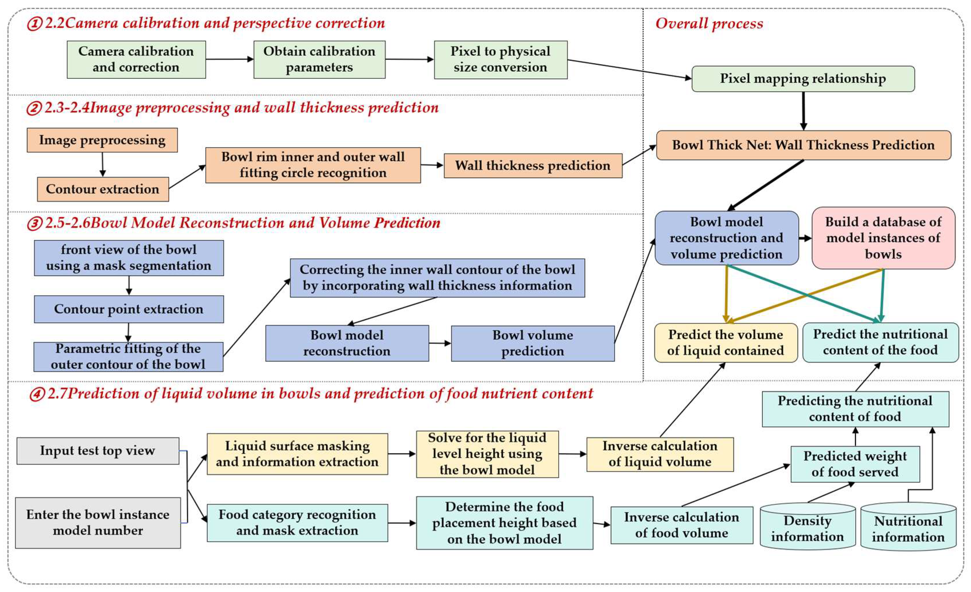
2.2. Camera Calibration and Perspective Correction
The frontal-view and top-down images of bowl-type tableware in this study were captured using a Hikvision (Hangzhou, China) MV-CS060-10UC-PRO industrial camera with a resolution of 3072 × 2048 and a maximum frame rate of 59.6 fps. Camera calibration is a critical step to ensure accurate estimation of tableware dimensions. Based on the pinhole camera model, we establish the mapping between pixel coordinates and world coordinates, thereby enabling dimensional measurement from 2D images to 3D models and compensating for errors caused by lens distortion. Variations in object distance induced by different camera models and settings may change the scale factor between image pixels and real-world physical units, thereby degrading measurement accuracy. To improve the precision of tableware dimension measurement, it is necessary to calibrate object-distance variations and compensate for height-related errors. Although the subsequent experimental images were , an industrial camera was chosen to ensure the stability and reproducibility of geometric measurements. Its low distortion, controllable intrinsic exposure, and ability to retain clear edges even after scaling from high-resolution acquisition are beneficial for accurate fitting and scale conversion. In contrast, mobile phones or ordinary cameras often employ implicit processing such as autofocus, auto exposure, multi-frame fusion, distortion correction, and food enhancement, which can easily introduce scale drift and edge distortion, reducing measurement consistency.
This paper adopts the planar calibration method proposed by Zhang, using a two-dimensional checkerboard calibration target with a side length of 25 mm. During the calibration process, 15 images of the calibration target are acquired by the camera at different heights and viewpoints (these 15 images are calibration images, not dataset samples), and the pixel coordinates of the checkerboard corner points are extracted [
11]. Subsequently, the homography matrix at each viewpoint is calculated to estimate the in-camera and out-of-camera pose parameters. Lens distortion parameters are further optimized using nonlinear least squares, and finally, maximum likelihood estimation is used to integrate the multi-view results to obtain stable calibration parameters. The above process is completed using the Camera Calibrator tool in MATLAB version R2019b, which establishes the mapping relationship between pixel coordinates and the true physical scale, providing a unified scale benchmark for subsequent geometric fitting and volume calculation, and reducing systematic errors caused by distortion.
In each calibration image, corner detection is performed to obtain the pixel coordinates of the checkerboard corners. We then solve for the mapping between the image pixel coordinates and the corresponding real-world geometric coordinates, thereby estimating the camera’s geometric parameters—including focal length, principal point, and intrinsic matrix—as well as its pose parameters, i.e., the rotation matrix, translation vector, and extrinsic matrix, together with the lens distortion coefficients [
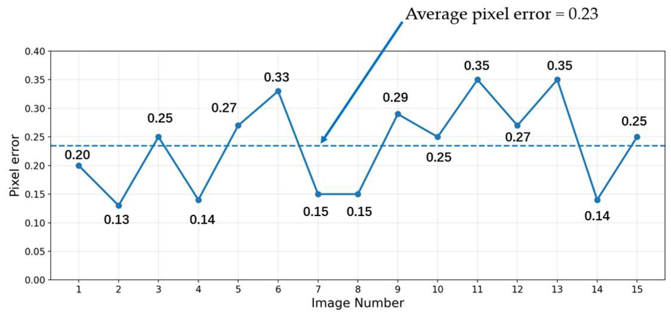
12]. These parameters determine the camera pose in the physical world, and the accuracy of the calibration model is verified by statistics of the reprojection error. In our experiments, the mean reprojection error is 0.23 pixels, indicating a small calibration error and ensuring the reliability of subsequent measurements.
Figure 2 shows the reprojection error statistics of the camera calibration.
During calibration, the checkerboard target was placed within the camera’s depth of field, and its pose was corrected using a spirit level and the camera pose parameters. Based on the established mapping between pixel and world coordinates, we obtained a pixel-to-world scale of when the camera-to-target distance was 954.325 mm and the image resolution was pixels. To facilitate subsequent image processing and bowl segmentation, the image resolution was resized to . Accordingly, the pixel-to-world mapping was adjusted using the scaling factor, yielding at a resolution of .
2.3. Image Enhancement and Preprocessing for Geometric Measurement
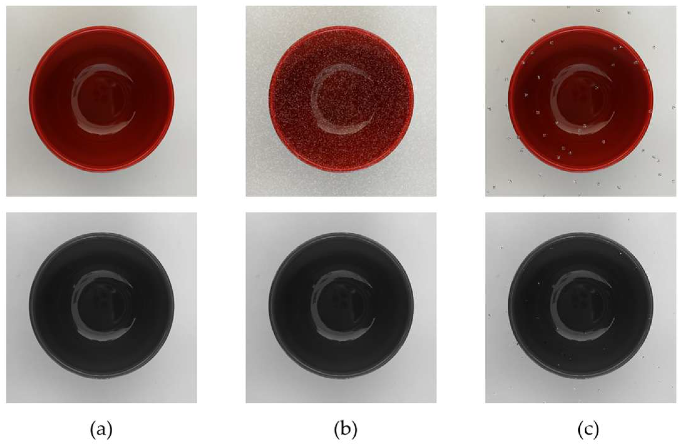
The outline of a bowl is usually composed of straight lines and arcs. Subsequent contour fitting and volume estimation are very sensitive to the accuracy of edge coordinates. Therefore, preprocessing needs to improve robustness without changing the pixel-to-physical scale mapping. In order to simulate common image degradation in actual acquisition, we simulated three phenomena that are easy to occur during shooting: local highlights (bright edges caused by specular reflection or direct light), salt and pepper noise (impact noise introduced by reflected flash, compression artifacts or transient interference), and random impulse noise clusters (bright and dark area clusters caused by electromagnetic interference or sensor transients). Through image comparison, we found that median filtering has a stronger ability to suppress the aforementioned outliers and impulse noise, and better preserves edge position and sharpness, thus providing a more stable input for contour segmentation, geometric fitting, and volume calculation [
13].
Figure 3 shows the image results of the three image degradation cases and the images after grayscale and median filtering.
In addition to the three types of degradation enhancements mentioned above, to improve the algorithm’s adaptability to changes in shooting conditions, we also adopted enhancement strategies that only change the grayscale distribution without altering the geometric relationships. These include small perturbations in brightness, contrast, and gamma, slight color jitter before grayscale processing, and moderate Gaussian noise and slight blurring. These do not change pixel coordinates and calibration scale, thus not disrupting the mapping relationship. Random scaling, cropping, rotation resampling, affine and perspective transformations, and non-uniform stretching directly change the relationship between pixels and physical scale, leading to systematic deviations in diameter, wall thickness, and volume integrals; therefore, they were not used in this experiment. To unify the processing flow and facilitate dataset construction, even the unenhanced original images underwent uniform grayscale conversion and median filtering. Since median filtering is a local, lightweight non-linear smoothing, it only introduces a small degree of pixel change in low-noise samples, but it can significantly improve the consistency of data across different batches and under different lighting conditions, as well as the robustness of subsequent contour extraction. Finally, both the front and top views of the bowl were preprocessed using a unified strategy of first grayscale conversion and then median filtering.
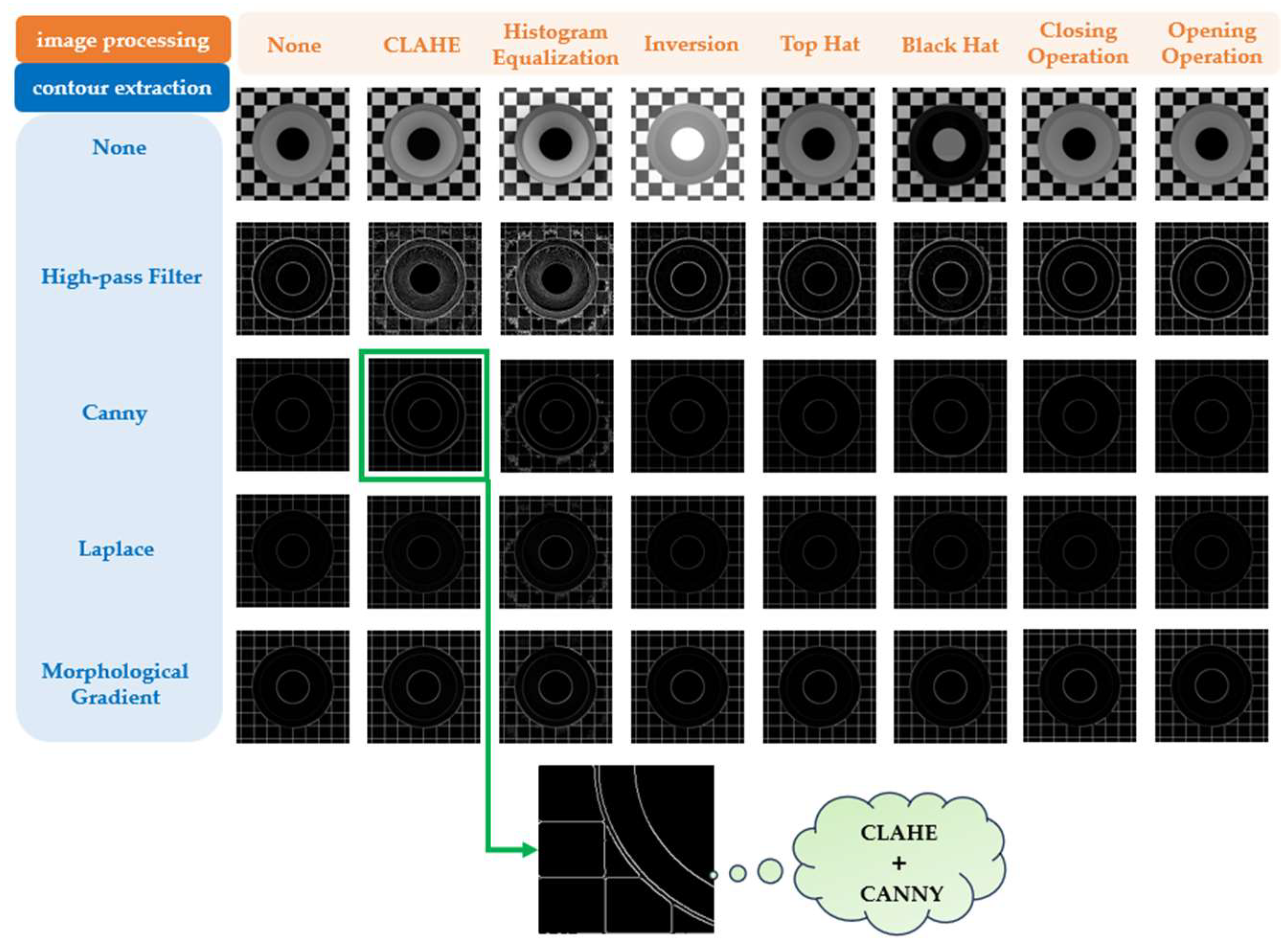
After filtering the frontal-view and top-down images, we extract the inner and outer rim contours from the top-down view to support subsequent bowl wall-thickness prediction. To this end, we design a two-stage pipeline consisting of (i) image processing and (ii) contour extraction. To evaluate the effectiveness of different method combinations, we tested 40 combinations (each comprising one image-processing method and one contour-extraction method). By visually inspecting and comparing the resulting images, we selected the optimal scheme for subsequent bowl wall-thickness prediction.
In stage (i), we apply seven common image-processing methods to enhance bowl contrast and improve contour separability. (a): CLAHE (Contrast Limited Adaptive Histogram Equalization) performs contrast-limited adaptive histogram equalization in local regions, enhancing low-contrast details and emphasizing bowl edges and specular highlights [
14]. (b): Histogram Equalization adjusts the global intensity distribution to alleviate uneven background illumination [
15]. (c): Inversion reverses pixel intensities to increase the visual distinction between the bowl and the background when their contrast is weak. In morphological processing [
16] (d): Top Hat transform enhances bright details and suppresses slowly changing background components by subtracting the opening operation result from the original images, thereby highlighting contour structures [
17]. (e): Black Hat subtracts the original image from the closed image to enhance dark-region details, which is beneficial when the bowl’s inner surface appears darker [
18]. (f): Closing Operation applies dilation followed by erosion to fill small gaps and holes, improving contour continuity. (g): Opening Operation applies erosion followed by dilation to remove small artifacts and isolated noise, producing cleaner images for subsequent contour extraction [
19].
In stage (ii), we employ four edge-detection techniques for contour extraction. (a): High-Pass Filter preserves high-frequency components to accentuate intensity transitions, thereby sharpening the bowl-rim contours [
20]. (b): Canny applies a multi-step procedure—including denoising, gradient computation, non-maximum suppression, and hysteresis thresholding—to stably extract the primary outer contours and edges while suppressing noise [
21]. (c): The Laplace localizes edges using the second-order grayscale derivative; although it is sensitive to noise, it provides complementary capability for capturing inner-wall details [
22]. (d): Morphological Gradient extracts contours by computing the difference between dilation and erosion, which is well suited to bowls with regular structures and distinct edges, highlighting the outer boundary while reducing interference from internal texture [
23].
By combining the stage-one image processing methods with the stage-two contour extraction methods, we processed the top-down images of bowls and obtained image-processing results for 40 different method combinations. The experimental results show that, as illustrated in
Figure 4, the combination of CLAHE and Canny significantly enhances the difference between the inner and outer walls, outperforming the other methods as well as the original image. Under this setting, both high-pass filter and Canny can extract the inner- and outer-wall contours; however, high-pass filtering is prone to adhesion. In contrast, Canny produces fewer breakpoints and branches, yields smoother contours, and provides clearer separation, making the processed top-down bowl images more suitable for subsequent bowl thickness prediction.
2.4. Bowl Wall Thickness Estimation Model—Bowl Thick Net
In bowl model reconstruction and capacity prediction, accurate estimation of geometric parameters is crucial, particularly because differences between the inner and outer wall structures affect the accuracy of capacity computation. In this section, circle localization is not performed directly on the original image but rather on the edge map after CLAHE and Canny edge extraction. Under this setting, the classic Hough circle transform can also be used for circle detection at the method level, but it usually outputs multiple sets of candidate circle responses, which may simultaneously cover arcs or circles formed by outer walls, inner walls, and other edge structures [
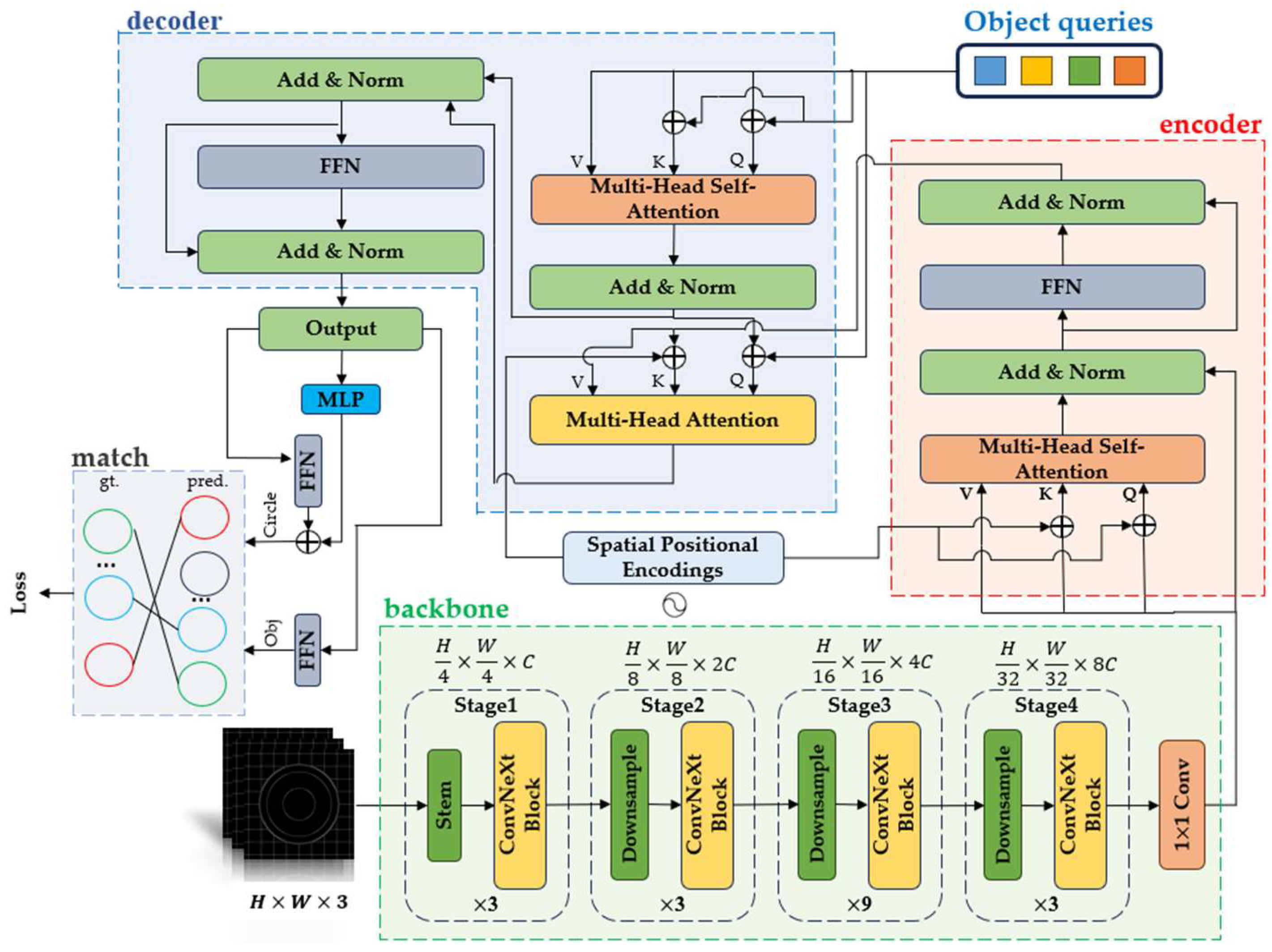
24]. To meet the task’s requirement of stably obtaining the largest outer circle and the second largest inner circle and outputting their corresponding geometric parameters, it is often necessary to have corresponding candidate selection and constraint strategies, such as radius range limitation, circle center consistency check, and deduplication and sorting. Based on the uniformity of the measurement process and the requirement of batch processing, this paper adopts a structured output learning method to directly predict and distinguish the largest and second largest circles, while outputting their geometric parameters, thereby reducing additional rule design and parameter processing, making subsequent contour fitting and volume estimation more consistent and reproducible. In this study, we adopt Conv NeXt-Tiny as the backbone network and use Res Net-18 as a baseline for comparison. We incorporate a Transformer-based framework with the Hungarian matching algorithm, and investigate the effects of Spatial Positional Encoding and Circle NMS (Circle Non-Maximum Suppression) on the recognition accuracy of the inner- and outer-rim contours at the bowl mouth [
25]. We design a Bowl Thick Net model that represents the inner and outer rim contours as two equivalent circles. The model detects the circular contours of the inner and outer rims in the top-down image and predicts bowl wall thickness from the size difference between the two fitted circles. This subsection details the feature extraction module, encoder–decoder architecture, post-processing, underlying principles, and experimental evaluation of the proposed model.
2.4.1. Feature Extraction for the Bowl Thick Net Model
In the feature extraction stage, the input consists of a batch of
RGB (Red Green Blue)top-down images of a bowl. Features are extracted using a backbone network, where we compare Conv NeXt-Tiny with Res Net-18; this subsection focuses on Conv NeXt-Tiny [
26]. Compared with the conventional Res Net-18, Conv NeXt employs convolutional operations such as depth wise convolution and pointwise convolution. Its hierarchical design from Stage 1 to Stage 4 progressively increases the channel dimension while reducing the feature-map resolution, thereby enhancing representational capacity. This design is particularly advantageous over Res Net-18 in capturing fine image details and higher-level features. The first layer is the stem, which maps the three-channel input to 96 channels, producing a feature map of size
. Stage 1 contains three Conv (Convolution) NeXt blocks and performs feature extraction via depth-wise separable and pointwise convolutions, reducing the feature map to
with 192 channels. Stage 2 contains three Conv NeXt blocks, reducing the feature map to
with 384 channels. Stage 3 contains nine Conv NeXt blocks, further reducing the feature map to
with 768 channels. Finally, Stage 4 extracts higher-level features and outputs a feature map of size
.
2.4.2. Spatial Positional Encodings
To enable the network to capture spatial location information—particularly for detecting circular geometric parameters—we explicitly incorporate PE (Positional Encoding) into the feature maps [
27]. Because the Transformer architecture is inherently not position-aware, we generate PE using 2D sine and cosine functions to ensure that the network can model spatial relationships across different locations. The formulations of the 2D sine and cosine positional encodings are given in Equations (1) and (2), respectively:
In this equation,
and
denote the row and column indices of a location in the feature map. Since the feature map size is
,
and
range from 0 to 19, i.e.,
. The variable
is the index of the positional-encoding dimension, and
is the positional-encoding dimensionality. The term
is used to control the frequency of the sine or cosine functions at different dimensions, so that the encoding of each position has different scales across dimensions, ensuring encoding diversity and strong positional discriminability.
The PE generated by the above equations is added element-wise to the backbone output feature map of size , yielding a position-aware feature map with the same size . The spatial resolution and channel dimension remain unchanged, while each spatial location now contains explicit positional information. The feature map is then flattened into a sequence of size , where 400 is the sequence length after flattening (). Specifically, each pixel in the feature map is converted into a 256-dimensional token, preserving spatial correspondence and providing the input for subsequent processing.
2.4.3. Encoder and Decoder
The encoder consists of six layers, each comprising a multi-head self-attention module and a FFN (Feed-Forward Network). In each layer, the input is processed with Add & Norm to ensure stable gradient propagation. The encoder outputs a tensor of size
, which is fed into the decoder and serves as the Key and Value in cross-attention. In the decoder, the inputs include the encoder output and 10 learnable object queries. Each query interacts with the encoded features through self-attention and cross-attention. Each decoder layer likewise contains multi-head self-attention and an FFN, with the central objective of generating the final predictions, including the circle center coordinates
and the circle diameter
. The regression is performed via two branches: the Circle Head, which predicts geometric attributes, and the Obj Head, which determines target existence [
28]. The predicted circular parameters are then de-normalized by mapping the coordinates and diameter from
back to pixel values, as shown in Equation (3):
In this equation,
,
, and
are the normalized outputs of the model, representing the normalized x-coordinate of the circle center, the normalized y-coordinate of the circle center, and the normalized circle diameter, respectively. All three values lie in the range
, and 640 denotes the input image resolution.
2.4.4. Post-Processing and Matching
In the post-processing and matching stage, to accurately match each predicted circle to its corresponding ground-truth circle, we employ the Hungarian matching algorithm to compute the matching cost between predicted and ground-truth circles. The cost matrix consists of a geometric loss and an existence loss. The geometric loss is measured using the Smooth L1 loss [
29], while the existence loss is computed using the BCE With Logits loss [
30]. The existence loss is defined in Equation (4):
In this equation,
denotes the number of samples, which here refers to the total number of detected circles.
is the ground-truth label for the
-th sample:
indicates that the circle corresponds to a target (i.e., the target exists), whereas
indicates that it is not a target (i.e., the target does not exist).
is the model’s raw prediction score for the
-th sample. This score can take any real value and is used to determine whether the sample is a target.
is the output of the sigmoid activation function, representing the probability that the
-th sample is a target by converting the raw score into a probability. By combining the geometric loss and the existence loss, we obtain the overall matching cost, as defined in Equation (5):
In this equation,
denotes the geometric loss and
denotes the existence loss.
and
are hyperparameters used to balance the respective contributions of the geometric and existence losses.
2.4.5. Circle NMS
Circle NMS is a critical step for handling multiple circle predictions, particularly when detecting the outer and inner rims of a bowl, where several predictions may be produced and some may be redundant or noisy. Circle NMS suppresses duplicate circles based on the distance between circle centers and the relative difference in diameters, ensuring that only the most accurate outer- and inner-rim predictions are retained [
31]. This procedure is essential for improving the stability and robustness of the model.
2.4.6. Principle of Bowl Thick Net for Wall-Thickness Prediction
The Bowl Thick Net model approximates the inner and outer rim contours at the bowl mouth as two circles. By detecting the two largest circular contours in the top-down image, it maps the predicted circle centers and diameters from the
range back to pixel values. Using the pixel-to-world mapping and the camera calibration parameters, the diameters of the two circles are then computed in real-world units. The bowl wall thickness is obtained by halving the difference between the two diameters. The corresponding formula is given in Equation (6):
In this equation,
denotes the bowl wall thickness,
is the diameter of the largest circle (the outer-wall rim contour), and
is the diameter of the second-largest circle (the inner-wall rim contour).
Figure 5 illustrates the architecture of Bowl Thick Net: Bowl Wall Thickness Estimation Network.
2.4.7. Experiments on the Bowl Thick Net Model
All images in the dataset were captured using an industrial camera under fixed height and illumination conditions, and were resized to to ensure accuracy and consistency. Experiments were conducted on Windows 10 using PyTorch 1.9.2, Python 3.8, CUDA 11.2, and an NVIDIA RTX 4060 GPU (Santa Clara, CA, USA). To enlarge the bowl image dataset, we applied data augmentation to expand the original 363 images to 1089 images. The dataset for this study was not entirely acquired in a checkerboard environment. In addition to checkerboard background samples, we also collected a large number of images that are closer to real-world application scenarios, including various backgrounds such as ordinary desktops and restaurant tables, to cover a wider range of textures and lighting conditions. The augmentation pipeline included a series of operations such as rotation, cropping, and flipping, while ensuring that these transformations did not alter the mapping between image pixels and physical dimensions. To maintain geometric consistency with the original images, each augmented image was further processed with CLAHE and Canny edge extraction to enhance contrast and edge features, facilitating subsequent contour detection and analysis. For bowls of different sizes and materials, we manually annotated the standard circle parameters of the outer and inner rims, and measured the bowl wall thickness using vernier calipers to construct millimeter-level ground-truth labels. The dataset was split into training and test sets at a ratio of 8:2.
To systematically evaluate the impact of each module on the performance of Bowl Thick Net, we designed eight model variants. The identifiers and meanings of these variants are as follows. Bowl Thick Net uses Conv NeXt-Tiny as the backbone and includes all modules, representing the final model performance when all components operate jointly. A replaces Conv NeXt-Tiny with Res Net-18 to assess the performance of a conventional convolutional network for bowl wall-thickness prediction. B removes Spatial Positional Encoding, such that the model can no longer explicitly exploit positional encoding to capture spatial relationships. C removes Circle NMS, performing no geometric deduplication and directly using the circle parameters output by the decoder. D–F each remove two of the three variables and retain only one, enabling analysis of the effect of a single remaining component. G removes all three variables to examine the maximum performance degradation when they are all absent.
Table 2 summarizes the modules used in each model variant.
All input images were normalized to and channel-wise standardized using ImageNet statistics. The backbone was initialized with ImageNet-pretrained weights. Both the encoder and decoder employed a 6-layer and a 8-head self-attention architecture, and the number of object queries was set to 10. In the loss function, the weight ratio between the geometric term and the existence term was set to 2:1, and the model was trained for 100 epochs. Optimization was performed using the SGD (Stochastic Gradient Descent) optimizer, and the mini-batch size and initial learning rate were tuned on the validation set. To improve robustness, early stopping and cross-validation were adopted during training to mitigate overfitting and ensure that the model effectively learns the key geometric features in the images.
A prerequisite for accurate bowl wall-thickness prediction is the correct identification of the two circular contours corresponding to the outer and inner walls in the image. We therefore evaluated the classification accuracy of the largest detected circle
(outer-wall contour) and the second-largest detected circle
(inner-wall contour) produced by the eight models on 218 test images; experiments on dimensional accuracy are reported subsequently. The results are summarized in
Table 3.
The results on the 218 test images are summarized in
Table 2. Bowl Thick Net achieves strong performance in classifying both the largest circle
(outer-wall contour) and the second-largest circle
(inner-wall contour). The recognition accuracy reaches 97.2% for
and 95.4% for
, and the proportion of test images in which both
and
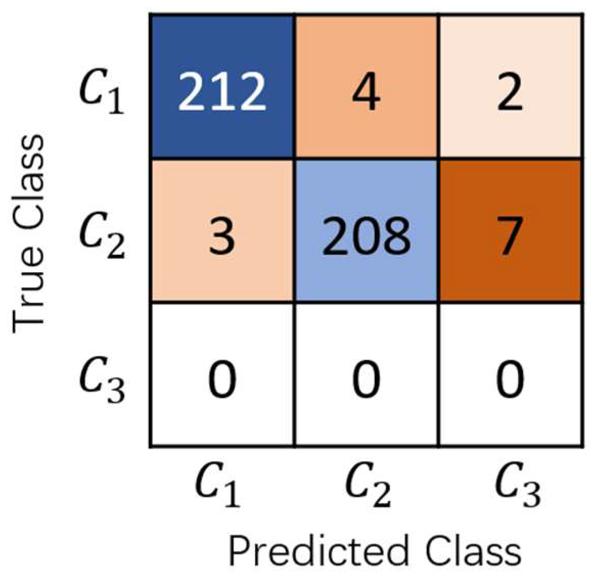
are correctly identified is 93.6%. The other model variants show slightly lower accuracies compared with Bowl Thick Net. In addition, the confusion matrix of Bowl Thick Net, which attains the highest recognition accuracy, is shown in
Figure 6, where
denotes circles other than
and
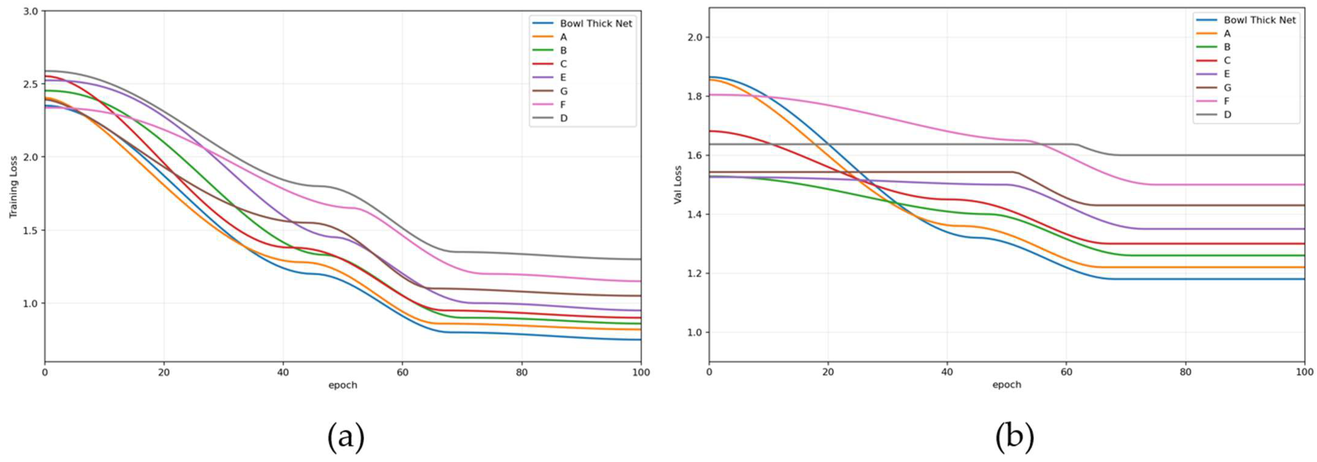
. To demonstrate the training stability and convergence behavior of Bowl Thick Net in identifying the largest outer circle
and the second largest inner circle
,
Figure 7 presents the loss curves for the training and validation sets. During training, the model uses the predicted circle parameters and circle existence as supervision signals, and the loss is composed of a weighted sum of a geometric regression term and an existence classification term. As the number of training epochs increases, both the training loss and the validation loss continuously decrease and tend to stabilize in the later stages. In the model, the accuracy of thickness prediction depends on the output parameters of the two circles. Therefore, when there is a discrepancy in the identification of the two circles, the error will propagate to subsequent prediction processes. Common identification failure scenarios include partial occlusion of the rim, edge loss due to reflection, and inaccurate fitting of multiple arc segments. In these cases, the model may misclassify non-target arcs as candidate circles, or the order of the two circles’ radii may become confused. To effectively handle these failures, we introduced a fault-tolerance mechanism into the workflow and added geometric consistency constraints to the outputs of the two circles. We require that the center positions of the two circles be consistent, and that the radii meet predefined order and range constraints. If the model detects that the output does not meet these geometric constraints, it will return to the previous identification step to readjust. In addition, we manually reviewed the low-confidence prediction results of the two circles to ensure that erroneous identification results do not affect subsequent volume derivation. Through these measures, we can effectively reduce the impact of identification failures in the thickness prediction stage, thereby improving the accuracy of the final volume estimation.
From the above model variants, we selected the output images in which both and were correctly identified to conduct experiments on the geometric size errors of the two circles. Since subsequent wall-thickness prediction requires only the circle diameters, we did not report the predicted circle-center coordinates. Instead, we de-normalized the predicted diameters to pixel values, computed the corresponding real-world diameters using the pixel-to-world mapping, and then calculated bowl wall thickness according to Equation (6). We report the predicted diameters of and and the resulting wall-thickness estimates for each model variant, and compare them with manual measurements.
In this study, we use
(Mean Prediction Error) to quantify the discrepancy between the model-predicted circle diameter or bowl wall thickness and the corresponding manual measurements.
computes the absolute error between the predicted and measured values for each image and then averages these errors over all images; a smaller value indicates closer agreement with the ground truth. We also report
(Mean Wall Thickness Prediction Accuracy), defined as the ratio between the predicted wall thickness and the manually measured wall thickness for each image, averaged across all images [
32]. This metric effectively reflects the model’s accuracy in wall-thickness prediction, with higher values indicating more accurate predictions.
Table 4 presents the predicted diameters of
and
and the resulting bowl wall-thickness estimates for each model variant. Bowl Thick Net achieves the best overall performance among all versions: the
for the diameters of
and
are 0.64 mm and 0.78 mm, respectively; the
for wall-thickness prediction is 0.75 mm, and the
is 73.3%. We further conducted capacity measurement experiments on multiple bowls. The results show that, using the wall-thickness predictions from this model, the percentage difference in capacity falls within 1.5–4%, demonstrating the effectiveness and accuracy of the proposed model in practical applications.
2.5. Mask Segmentation of Bowls
In this subsection, we use the frontal-view images paired with the bowl top-down images as input and adopt Mask R-CNN as the base framework. Since each image contains only a single bowl, the primary goal is to obtain a high-quality mask with smooth boundaries and accurate details. However, the standard Mask R-CNN, which is designed for multi-object and multi-class detection, introduces redundant computation and may provide insufficient contour delineation for our task [
33]. To address this issue, we build an improved Mask R-CNN framework and compare three backbone networks. We further propose a geometry-aware feature pyramid structure, GFPN (Geometry-aware Feature Pyramid Network), tailored to this study, and investigate its effect on bowl mask segmentation. Finally, we select the model with the highest segmentation accuracy and extract keypoints from the predicted bowl mask to infer the rim diameter, base diameter, bowl height, and the sidewall contour corrected by the predicted wall thickness, which are then used to estimate bowl capacity.
2.5.1. Improved Mask R-CNN Framework
In this subsection, we propose an improved Mask R-CNN baseline that is optimized for the characteristics of the mask segmentation task. Conventional Mask R-CNN is primarily designed for multi-object, multi-class detection and must jointly support classification and detection, which leads to substantial computational overhead on classification and insufficient delineation of fine bowl contours. To address these issues, we retain the two-stage architecture and the mask branch, while improving the feature extraction and pyramid fusion components. For region proposal generation, we continue to use the RPN (Region Proposal Network) [
34]. However, considering the single-bowl image setting and the requirement for high geometric precision, we simplify the RPN structure and its output configuration. At each scale, we keep only a small set of scale and aspect-ratio combinations that better match bowl contours, thereby reducing the number of proposals and improving convergence efficiency. Standard Mask R-CNN produces hundreds of proposals and then filters them via NMS before further processing; in our task, this is redundant and may introduce uncertainty. Therefore, after NMS we retain only 50–100 high-confidence proposals and feed them into RoI Align (Region of Interest Align) and the segmentation head for subsequent processing. In the RoI (Region of Interest)head, we perform single-class classification without distinguishing specific bowl types [
35]. This avoids allocating additional fully connected layers and classification losses for fine-grained categorization. Meanwhile, we keep the original loss functions, which helps the feature representations in the mask and geometric branches remain more focused, thereby improving contour segmentation accuracy.
2.5.2. Three Different Backbone Networks
For the backbone, we adopt three architectures—Res Net-50, Res NeXt-50 (32 × 4d), and Res Net-C4—to maintain compatibility with the standard Mask R-CNN and to facilitate controlled comparisons. The reasons for selecting these three backbones are as follows:
Res Net-50 serves as the baseline for comparison. By introducing residual blocks and skip connections, it effectively alleviates the vanishing-gradient problem in deep networks [
36].
Res NeXt-50 (32 × 4d) can be regarded as augmenting the Res Net-50 bottleneck with 32 parallel 3 × 3 convolutional groups, each with 4 channels, implemented via grouped convolutions, thereby improving texture representation and contour modeling capability [
37].
Res Net-C4 retains only C1–C4 as the shared backbone and does not further down sample to C5, trading some high-level semantic information for higher spatial resolution and finer local structure, which benefits precise localization of geometric boundaries such as the bowl rim and base [
38].
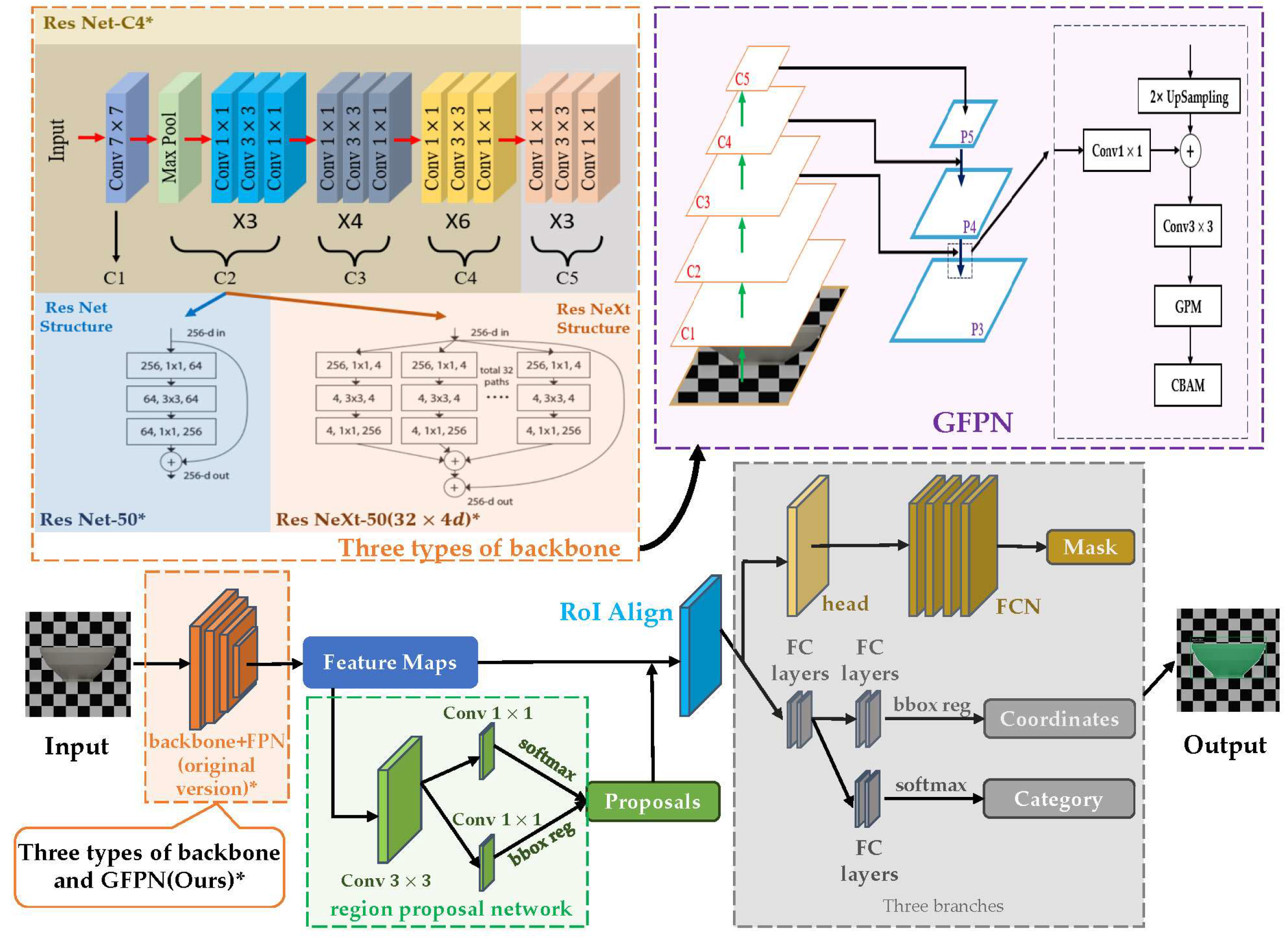
The architectures of the three backbones are illustrated in the upper-left part of
Figure 8. The three boxes correspond to the three backbone variants. Beneath C2, using C2 as an example, the figure further compares the convolutional operation in Res Net-50 with standard convolutions against that in Res NeXt-50 (32 × 4d) with grouped convolutions. By comparing these three backbones, we can analyze how backbone architecture affects mask quality and geometric fitting accuracy.
2.5.3. Geometry-Aware Feature Pyramid Network
The FPN (Feature Pyramid Network) is a multi-scale architecture widely used in object detection [
39]. It enhances the recognition of targets at different scales by fusing feature maps from multiple hierarchical levels in a bottom-up pyramid manner. In our task, FPN plays the following roles:
Improved contour segmentation accuracy: Because bowl contours may exhibit subtle variations, FPN effectively combines fine-grained details from shallow layers with high-level semantic information from deeper layers, thereby improving the accuracy of bowl contour segmentation. In particular, for segmenting the bowl rim and base, FPN strengthens the model’s sensitivity to fine details, ensuring accurate extraction of circular contours.
Reduced computational redundancy: In conventional Mask R-CNN, processing multi-scale features can introduce redundant computation. FPN mitigates this issue through efficient feature fusion, improving computational efficiency. This advantage is especially important for bowl segmentation tasks that require real-time performance or high-throughput processing.
Multi-scale feature extraction: FPN extracts features at different hierarchical levels and fuses them, enabling the model to recognize targets at various scales within the image.
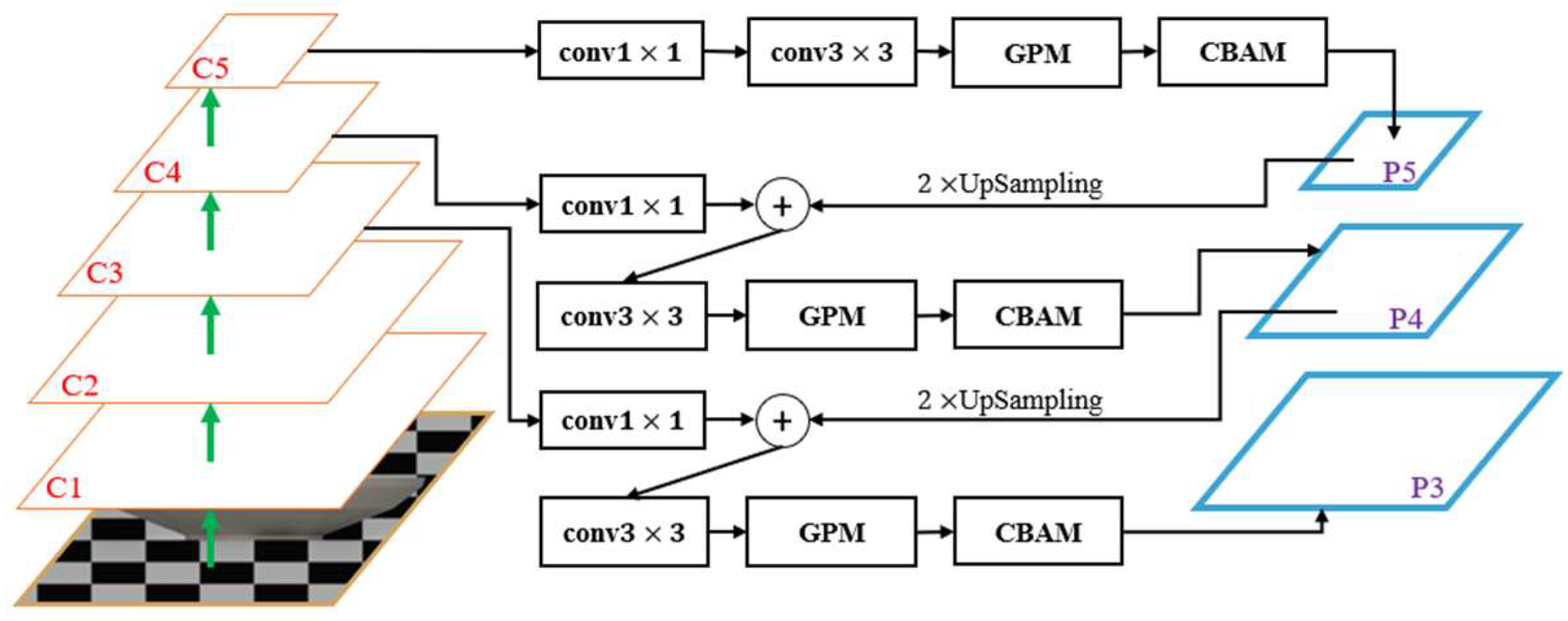
To further emphasize bowl contour features, we propose a Geometry-aware Feature Pyramid Network (GFPN) that includes only P3–P5, built on the C3–C5 outputs of Res Net-50 and Res NeXt-50 (32 × 4d). This pyramid follows the standard top-down design with convolutions, up sampling, and convolutions. On this basis, we introduce a GPM (Geometry-aware Prior Modulation) module and the CBAM (Convolutional Block Attention Module) attention mechanism. With multi-scale feature enhancement, GFPN strengthens boundary responses and thereby improves the accuracy of bowl contour segmentation.
GPM enhances the model’s understanding of geometric structures by incorporating geometric prior knowledge. In mask segmentation, GPM modulates the feature maps according to the geometric shape information in the input image, thereby improving sensitivity to geometric boundaries such as bowl contours [
40]. CBAM strengthens feature representation through two components: channel attention and spatial attention. Channel attention models the importance of each channel and selectively amplifies informative channel features, whereas spatial attention emphasizes different spatial locations to increase the model’s responses to salient regions [
41]. GFPN is derived from the original FPN with targeted modifications. The overall architecture of GFPN is shown in
Figure 9, and the procedure is described as follows:
The frontal-view bowl image is first converted to grayscale, and the resulting grayscale image is denoted as
. The corresponding morphological gradient image is defined in Equation (7):
In this formulation,
takes larger values near the bowl contour and is close to zero in background regions, where
and
denote the height and width of the original image. To inject scale-matched geometric priors into each FPN level,
is downsampled at multiple scales and encoded via convolution. Taking the third level with a stride of 8 as an example, average pooling is first applied to obtain a coarse-scale boundary map
, which is then encoded using a
convolution to produce the geometric prior feature
. The details are given in Equations (8) and (9):
In these equations,
denotes the coarse-scale boundary map at the third level,
represents the average pooling operation, and
and
.
In these equations, denotes the geometric prior feature corresponding to a stride of 8. is a function symbol representing the convolution operation, which transforms the input map into a new feature map . denotes a convolution.
Similarly, for the levels with strides of 16 and 32, the corresponding geometric prior features and can be obtained. Thus, for the three levels with strides of 8, 16, and 32, we derive the geometric prior features , , and . These features are spatially aligned with the backbone outputs C3–C5 and serve as the geometric priors for their respective levels.
For feature fusion, we adopt a top-down pathway and retain only P3–P5, which match a single, medium-scale bowl target. Let the backbone outputs at C3, C4, and C5 be
,
, and
, respectively. The top-level pyramid output
is first obtained by applying
and
convolutions to
to produce the base fused feature
, as defined in Equation (10):
In these equations,
denotes the channel-compressed top-level feature, and
denotes the base fused feature at the top level.
and
represent
and
convolutions, respectively. For the intermediate level, taking the fourth backbone output
as an example, we first apply a
convolution to
. We then upsample the pyramid feature
by a factor of two so that its spatial resolution matches that of C4. The two features are added element-wise and passed through a
convolution to obtain the base fused feature for this level. This process is defined in Equations (11) and (12):
In these equations,
denotes the channel-compressed feature at the fourth level.
denotes a two-fold up sampling operation; here, it upsamples the pyramid output from the upper level—
in this example—by a factor of two, producing the upsampled feature
.
In these equations,
denotes the fused feature obtained by element-wise addition at the fourth level, and
denotes the base fused feature at this level. Subsequently, the GPM module applies a
convolution followed by a sigmoid activation to each level’s geometric prior feature
to produce a normalized geometric weight map. This weight map modulates the base feature
in a residual manner, yielding the geometry-modulated feature map
at level
. The process is defined in Equations (13) and (14):
In these equations,
denotes the pyramid level (here,
to
).
is the normalized geometric weight map at level
,
denotes the sigmoid function,
denotes the convolution operator,
is a
convolution kernel, and
is the geometric prior feature at level
.
In these equations,
denotes the pyramid level (here,
to
).
is the feature map at level
after geometric prior modulation.
denotes the geometric prior modulation module.
is the base feature at level
, and
is the geometric prior feature at the same level.
denotes element-wise multiplication, and
is the normalized geometric weight map for level
.
Finally, we apply the CBAM module to
to adaptively reweight the features along both the channel and spatial dimensions, producing the geometry-aware pyramid output
. This process is given in Equation (15):
In this equation,
denotes the pyramid level (here,
to
).
is the geometry-aware pyramid output at level
, and
denotes the CBAM module.
2.5.4. Bowl Mask Segmentation Model Process
This subsection summarizes the overall workflow of the proposed bowl mask segmentation model based on an improved Mask R-CNN. First, we adopt the improved Mask R-CNN as the baseline framework. To meet the requirements of single-bowl images and high geometric precision, we optimize region proposal generation and introduce the GFPN structure to strengthen the model’s sensitivity to bowl contours. By incorporating the GPM module and the CBAM attention mechanism, the model can more accurately capture fine-grained features of the bowl rim, base, and sidewall. To further improve segmentation accuracy, GFPN enhances the bowl’s geometric boundaries across multiple scales and performs feature fusion on the outputs of the C3–C5 layers. With these optimizations, the model effectively reduces background noise interference and improves the accuracy of bowl contour segmentation.
Figure 8 illustrates the architecture of the improved bowl mask segmentation model.
2.5.5. Experimental Results and Analysis
In this experiment, we use 363 frontal-view images of bowls that were captured together with the corresponding top-down images, and expand the dataset to 1089 images through data augmentation. The dataset includes bowls of various sizes. All images were manually annotated using the LabelMe tool version 5.8.1, and converted to the standard COCO annotation format. Unlike the original COCO setting, this task does not involve bowl-type classification; therefore, all instances are labeled as a single class, while still retaining bounding boxes and segmentation masks. The hardware and software settings are the same as those in
Section 2.4. Each image has an original resolution of
pixels. The dataset was randomly split, with 80% of the data used for training and 20% used for testing.
In this study, we adopt a Mask R-CNN model pre-trained on the COCO dataset and fine-tune it by loading the corresponding pre-trained weights. To improve accuracy and efficiency, we adjust the RPN_ANCHOR_SCALES parameter to (16, 32, 64, 128, 256) to better accommodate feature extraction for smaller image sizes. The initial learning rate is set to 0.0005, with a momentum of 0.9, weight decay of 0.00005, a batch size of 8, and 100 training epochs to ensure stable optimization on the reduced image resolution. During training, we use a stepwise learning-rate decay schedule, reducing the learning rate by a factor of 0.1 every 15 epochs. To further improve training stability and convergence speed, we employ a staged training strategy. In the early stage, the first several layers of Res Net are frozen and only the subsequent layers are trained, allowing the network to focus on task-relevant features. As training progresses, more Res Net layers are gradually unfrozen, ultimately enabling end-to-end optimization of all layers.
For model evaluation, we adopt COCO-style segmentation metrics, including
(Intersection over Union),
(Mean Intersection over Union),
(Average Precision), and
(Mean Average Precision) [
42,
43]. Specifically, in this experiment,
is defined as the ratio between the area of intersection and the area of union of the predicted mask and the ground-truth mask, and
is the average
over all images. Since our task involves segmentation of only a single class,
is equivalent to
as used in multi-class settings. The calculation is given in Equation (16):
To quantify the model’s boundary prediction accuracy, we evaluate it using the
with a 3-pixel tolerance. This metric assesses boundary performance by computing
, defined as the proportion of the predicted boundary that overlaps the ground-truth boundary, and
, defined as the proportion of the ground-truth boundary that overlaps the predicted boundary [
44]. The final
is the weighted harmonic mean of
and
, as given in Equation (17):
In this experiment, we report and at two thresholds, 0.50 and 0.75, as well as the mean and averaged over these two thresholds. The corresponding metrics are , , , , , and , together with the .
To systematically evaluate the effects of different backbones and the proposed GFPN on bowl mask segmentation performance, we conduct a comparative study based on the improved Mask R-CNN baseline with different configurations. Three representative residual-network backbones are considered: Res Net-50, Res NeXt-50 (32 × 4d), and Res Net-C4. Here, Res Net-C4 serves as a shallower backbone without FPN, whereas the other two backbones are equipped with either the standard FPN or the proposed geometry-aware feature pyramid GFPN. All models are trained and evaluated on the same grayscale-processed frontal-view bowl dataset using the metrics described above.
Table 5 Experimental results of mask segmentation of bowls in models of different modules.
Under the same experimental settings and hyperparameters, we select the best-performing configuration described above—using Res NeXt-50 (32 × 4d) as the backbone and GFPN as the FPN type—which we refer to as Ours, and compare it with other mask segmentation models, including U-Net, HTC, and B Mask R-CNN. All baseline models are evaluated using their original architectures without any module modifications. U-Net employs skip connections to fuse multi-scale features, balancing global semantics and local boundary details for pixel-level mask prediction [
45]. HTC alternately optimizes the detection and mask branches and progressively refines predictions through a multi-stage cascade, improving localization and segmentation quality [
46]. B Mask R-CNN is a boundary-enhanced variant of Mask R-CNN that introduces contour supervision and feature enhancement to strengthen edge representations and improve mask boundary accuracy and consistency [
47].
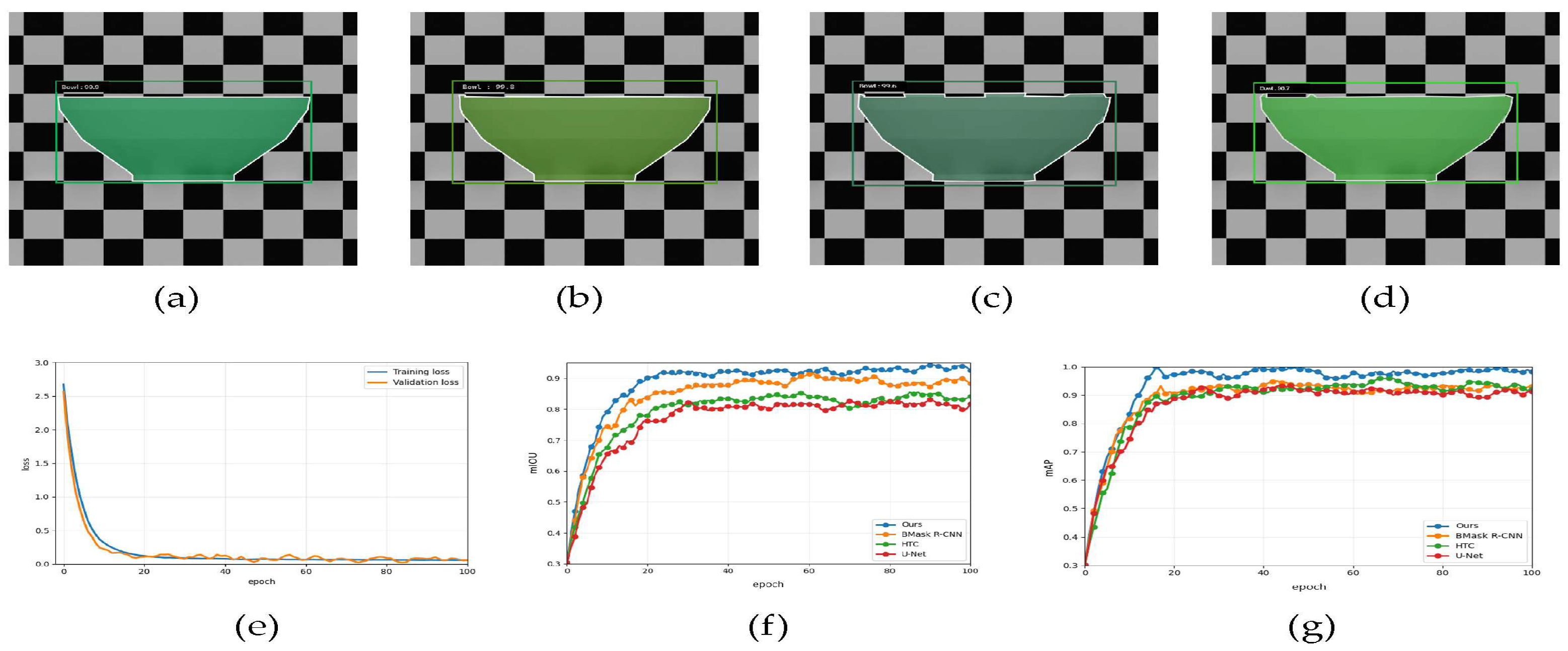
Table 6 reports the comparative results of these four models.
Figure 10 presents qualitative segmentation outputs for all models, along with the training and validation loss curves of our model and the
and
curves of the four models.
2.6. Estimation of the Volume of a Bowl
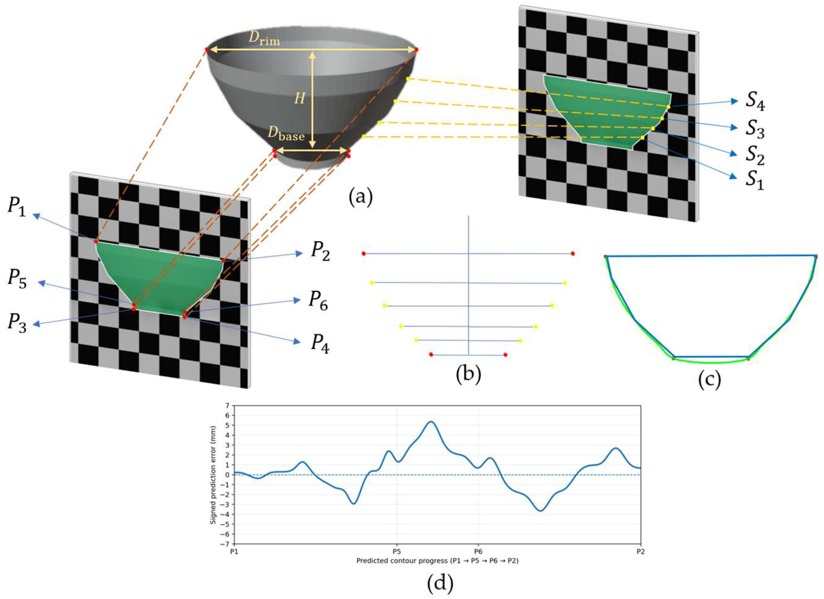
After obtaining the bowl mask, we use the segmentation model from the previous subsection and define 10 geometric key points on the mask: the outer-contour extremal points
and four uniformly sampled points along the right-side arc length,
. These keypoints are used to derive the rim diameter, base diameter, and bowl height, and to fit the inner-wall contour by incorporating the predicted wall thickness [
48]. Finally, the bowl volume is computed via axisymmetric integration. The detailed procedure is as follows:
1. Foreground pixel set and contour set: After bowl mask segmentation, let the binary mask be
. We first construct the foreground pixel set and the contour set on the mask, which are used for subsequent definition of geometric keypoints and fitting of the outer-wall curve, as given in Equation (18):
In this equation,
denotes the set of foreground pixels in the mask image.
is the mask value at pixel
, where the foreground is 1 and the background is 0, and
and
are the horizontal and vertical pixel coordinates in the image coordinate system.
denotes the contour set extracted using OpenCV’s contour detection.
2. Six outer-contour extremal points
: To stably obtain the geometric boundaries of the bowl rim and base from the mask contour, we define four extremal points on
: the left and right upper-rim points
and
, and the left and right lower-base points
and
. The upper-rim points characterize the rim width, whereas the lower-base points characterize the base width and help determine the base position. Their definitions are given in Equations (19) and (20):
In this equation,
and
denote the minimum and maximum horizontal coordinates on the contour set
, respectively.
denotes the point within the specified domain that maximizes the objective function.
and
correspond to the left and right upper-rim points, respectively. Specifically,
and
are the highest points in the leftmost and rightmost contour columns, respectively.
In this equation,
denotes the point within the specified domain that minimizes the objective function.
and
correspond to the left and right lower-base points, respectively. Specifically,
and
are the lowest points in the leftmost and rightmost contour columns, respectively.
Because the base primarily provides structural support and does not contribute to the effective holding volume, directly using
and
would lead to an overestimation of bowl height. Therefore, we analyze the variation in the mask’s horizontal width along the vertical direction to locate the shape transition between the base and the bowl body. The left and right boundaries at this transition are defined as
and
, which are used for estimating the effective height and fitting the sidewall. The definition is given in Equation (21):
In this equation,
denotes the foreground width of the mask at row
, and
and
are the rightmost and leftmost horizontal coordinates of the foreground region at row
, respectively.
In the base region,
varies only slightly, whereas once entering the bowl body sidewall,
increases markedly as
increases. We scan upward from the base and identify the first row at which the width change rate exceeds a threshold
, denoted as
. In our implementation,
is set to 5 px, and the left and right boundary points at this split row are defined as
, as given in Equation (22):
In this equation,
is the pixel
-coordinate of the height where the base transitions to the bowl body.
is the left boundary point at the start of the bowl body after removing the base, and
is the corresponding right boundary point.
3. Pixel-scale geometric quantities: rim diameter, base diameter, and effective height. After obtaining the keypoints
, we can directly compute the bowl rim diameter, base diameter, and effective height in pixel units. The pixel-scale rim diameter is defined in Equation (23):
In this equation,
denotes the rim diameter in pixels, and
and
are the horizontal coordinates of points
and
, respectively. The pixel-scale base diameter is defined in Equation (24):
In this equation,
denotes the base diameter in pixels, and
and
are the horizontal coordinates of points
and
, respectively. The bowl’s effective height uses the midpoint of the rim as the upper reference point and the base–body split line defined by
and
as the lower reference, thereby reducing the influence of the base height. The pixel-scale effective height is defined in Equation (25):
In this equation,
denotes the effective bowl height in pixels, and
,
,
, and
are the vertical coordinates of
,
,
, and
, respectively.
4. Conversion from pixel units to physical scale: Using the pixel-to-world mapping obtained in
Section 2.2,
, we convert the pixel-scale measurements to real-world dimensions, including the rim diameter
, base diameter
, and bowl height
. The conversion is given in Equation (26):
In this equation,
,
, and
denote the rim diameter, base diameter, and bowl height in real-world units, respectively, while
,
, and
denote the corresponding measurements in pixel units.
5. Sampling the right-side outer contour: Since a bowl can be approximated as an axisymmetric solid generated by rotation about its central axis, we model the bowl using the right-side outer contour. Specifically, we select the contour arc segment from
to
and denote the contour point sequence as
. Using arc-length parameterization, we uniformly sample four interior points
along this arc. Together with the endpoints
and
, these points form a representative set that characterizes the outer-wall shape, as defined in Equation (27):
In this equation,
denotes the arc-length increment between adjacent contour points.
and
are the horizontal and vertical coordinates of the
-th point, and
and
are defined analogously. Here,
is the contour-point index ranging from 1 to
, where
is the total number of contour points.
represents the cumulative arc length from the starting point
to the
-th point.
denotes the arc-length increment between the
-th point and the
-th point, where
is the summation index ranging from 1 to
.
is the arc length at the starting point and is set to 0.
denotes the total arc length from the starting point
to the endpoint
, i.e., the full length of the selected contour segment. We then select four interior point locations by dividing the arc-length interval
into five equal parts, as defined in Equation (28):
In this equation,
denotes the arc-length position of the
-th sampled point, where
is the sampling index and takes values from 1 to 4. By performing linear interpolation on
at
, we obtain the sampled point
, i.e., the coordinates of
.
6. Outer-wall fitting and inner-wall correction: To convert the contour points into a continuous geometric representation, we determine the bowl’s central axis using the midpoint of the rim and project the right-side sampled points onto the height–radius plane. In physical units, we fit the outer-wall radius function
. We then combine this with the wall thickness
predicted by Bowl Thick Net to obtain the inner-wall radius function
, as defined in Equation (29):
In this equation,
denotes the outer-wall radius as a function of height
, and
denotes the inner-wall radius as a function of height
. The coefficients
,
,
, and
are obtained via least-squares fitting.
7. Bowl capacity via axisymmetric integration: After obtaining the inner-wall profile
, we compute the bowl’s inner-cavity volume using the volume-of-revolution formula. The integration limits correspond to the effective height range, starting from the height of
at the bottom and ending at the rim at
. The formulation is given in Equation (30):
In this equation,
denotes the bowl capacity,
and
are the lower and upper bounds of the effective height in physical coordinates, and
is the inner-wall radius function.
In summary, based on the frontal-view bowl images, we use the outputs of our improved mask segmentation model to extract key geometric parameters, including the rim diameter, base diameter, and bowl height. By further incorporating the wall thickness predicted by Bowl Thick Net, we construct axisymmetric contour curves for the inner and outer walls, derive an integral formulation for bowl capacity, and complete the bowl reconstruction model.
Figure 11 illustrates the bowl capacity estimation procedure and the corresponding results.
Following the above pipeline, we conduct a capacity validation experiment on eight bowls of different sizes.
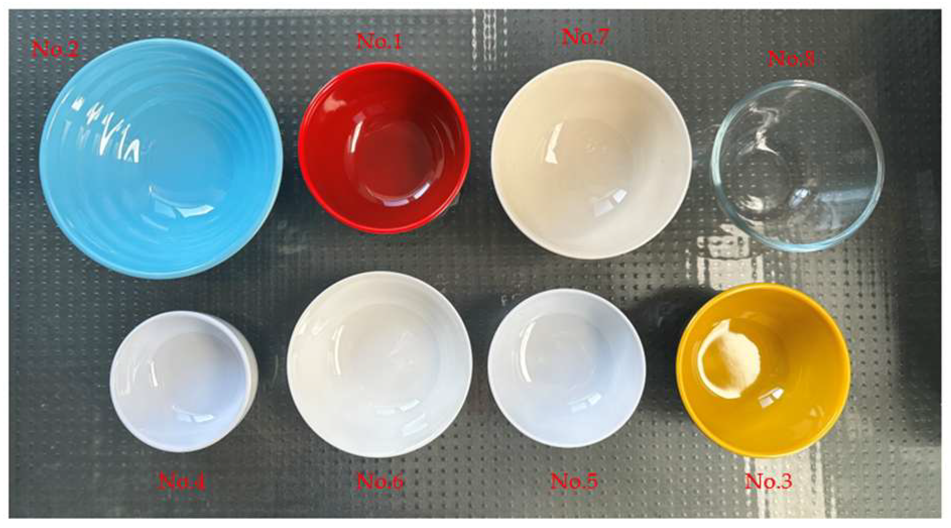
Figure 12 shows examples of real-world images of eight bowls used for prediction. These bowls vary in color, material, and size and are presented in a focused comparison to visually demonstrate the applicability and generalization ability of the scale factor and geometric modeling process used in this study with different bowl shapes.
For each bowl, we first acquire a top-down image and a frontal-view image. The rim contour in the top-down image is used to predict wall thickness, while the mask and contour point set from the frontal-view image are used to obtain the bowl’s geometric parameters and contour curve. The outer-wall contour is then corrected to the inner-wall contour, yielding image-based geometric parameters, a reconstructed bowl model, and the predicted bowl capacity. As ground-truth references, we manually measure the rim diameter, base diameter, effective height, and actual holding volume of each bowl using tools such as vernier calipers (Shanghai, China) and a graduated cylinder (Yancheng, Jiangsu, China). Finally, we evaluate the accuracy of the proposed bowl model reconstruction and volume estimation method by comparing the predicted and measured geometric dimensions and capacities of the eight bowls on a per-bowl basis and conducting error analysis.
Table 7 presents the measured and predicted values of rim diameter, base diameter, effective height, and bowl capacity for each bowl.
As shown in
Table 7, the prediction error for the rim diameter of the bowl ranges from 2.19% to 4.67%, with an arithmetic mean error of 1.09%. For the base diameter of the bowl, the error ranges from 1.03% to 3.42%, with an arithmetic mean error of 1.14%. For the effective height of the bowl, the error ranges from −2.26% to 1.03%, with an arithmetic mean error of 0.40%. For the bowl volume, the error ranges from −7.29% to 3.41%, with an arithmetic mean error of −3.03%. To further analyze the impact of network structure selection on the accuracy of bowl volume prediction, we conducted a comparative experiment between the backbone network and the feature pyramid structure, as shown in
Table 8. While keeping other training settings consistent, we compared the impact of different backbones and FPN types on the final volume error, using the arithmetic mean error of the bowl volume as a unified metric.
2.7. Application of This Study in Dietary Analysis
After obtaining the key geometric parameters of each bowl (rim diameter, base diameter, effective height, and capacity) and its reconstructed model, we store these parameters together with the corresponding bowl ID in a database, which serves as prior knowledge for subsequent prediction of liquid volume and food nutrient content. In practical use, the system first selects the bowl with the specified ID and captures a top-down image of the liquid or food in the bowl. To ensure consistent scale conversion and geometric mapping, the camera parameters, mounting height, and top-down viewing angle must be kept strictly identical to those used during the acquisition of the bowl top-down images described above. Next, the visible upper-surface region of the contents is segmented to obtain its top-down projection, and a circle is fitted to this region to estimate the diameter of the fitted surface circle. Combined with the inner-wall contour function of the selected bowl stored in the database and the corresponding cavity geometry constraints, this diameter can be mapped to the associated height, enabling inference of the liquid level and computation of the liquid volume via integration. Please note that this volume estimation assumes the upper surface of the liquid or food is as horizontal as possible; pronounced concavities, bulges, or stacked structures may introduce additional error. For food nutrient prediction, the system can estimate nutrients for a single food type. After estimating food volume, density is introduced to convert volume to weight, and the nutrient content (e.g., calories, carbohydrates, protein, and fat) is then obtained by linear scaling based on a per-unit-weight nutrient table for different dishes, yielding the estimated nutrient amounts for the food in the bowl [
49,
50].
2.7.1. Prediction of the Volume of Liquid in the Bowl
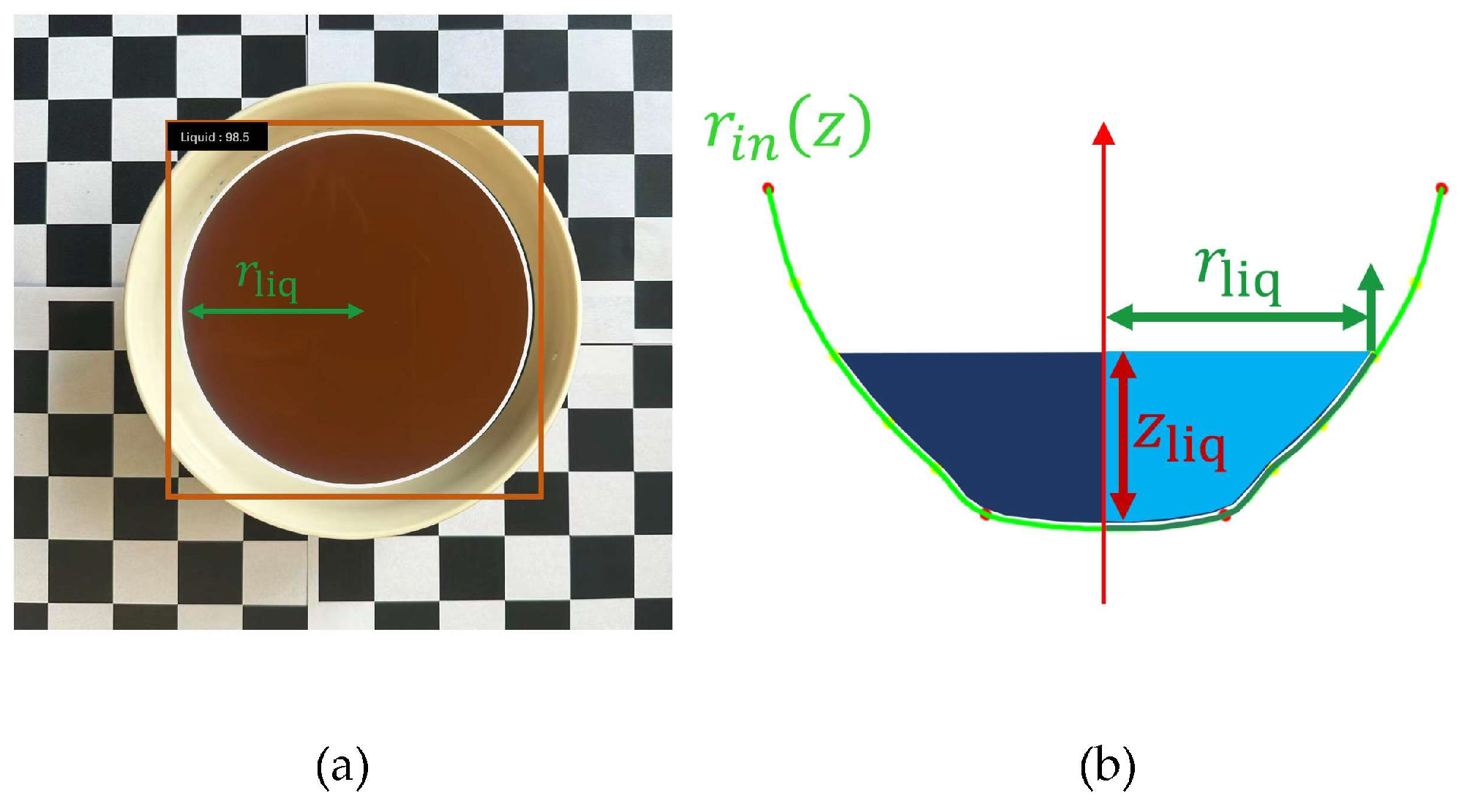
After completing bowl mask segmentation and obtaining the bowl geometric parameters as described in the previous subsection, we have the rim diameter , base diameter , and effective height in physical units, as well as the inner-wall radius function , which is obtained by fitting the outer wall and then correcting it using the predicted wall thickness. Specifically, denotes the height coordinate along the bowl’s central axis, and is the radius from the inner wall to the central axis at height . Under the axisymmetry assumption, the bowl cavity can be regarded as a solid of revolution generated by rotating about the central axis. Therefore, when the liquid level is as horizontal as possible, the liquid volume can be computed by integrating the volume of revolution below the liquid level.
We perform mask segmentation on the surface region in the top-down liquid image and fit an equivalent circle to the liquid-surface contour to obtain the pixel-scale radius
. Using the calibration factor
(mm/pixel) we convert it to the physical liquid-surface radius
, as given in Equation (31):
Since the inner-wall profile is represented as a continuous function
, the liquid level can be inferred from the liquid-surface radius. In implementation,
is interpolated within the integration interval defined by the effective height, and the corresponding
is solved using a bisection method. The liquid-surface radius
and the liquid level
satisfy Equation (32):
After determining the liquid level
, the liquid volume is computed as the volume of revolution from the bottom
up to
, as given in Equation (33):
In this equation,
denotes the predicted liquid volume in
.
Figure 13 illustrates the liquid mask segmentation and the principle of liquid volume prediction.
2.7.2. Predicting the Nutritional Content of Food in a Bowl
After obtaining the bowl’s geometric parameters and the inner-wall contour function
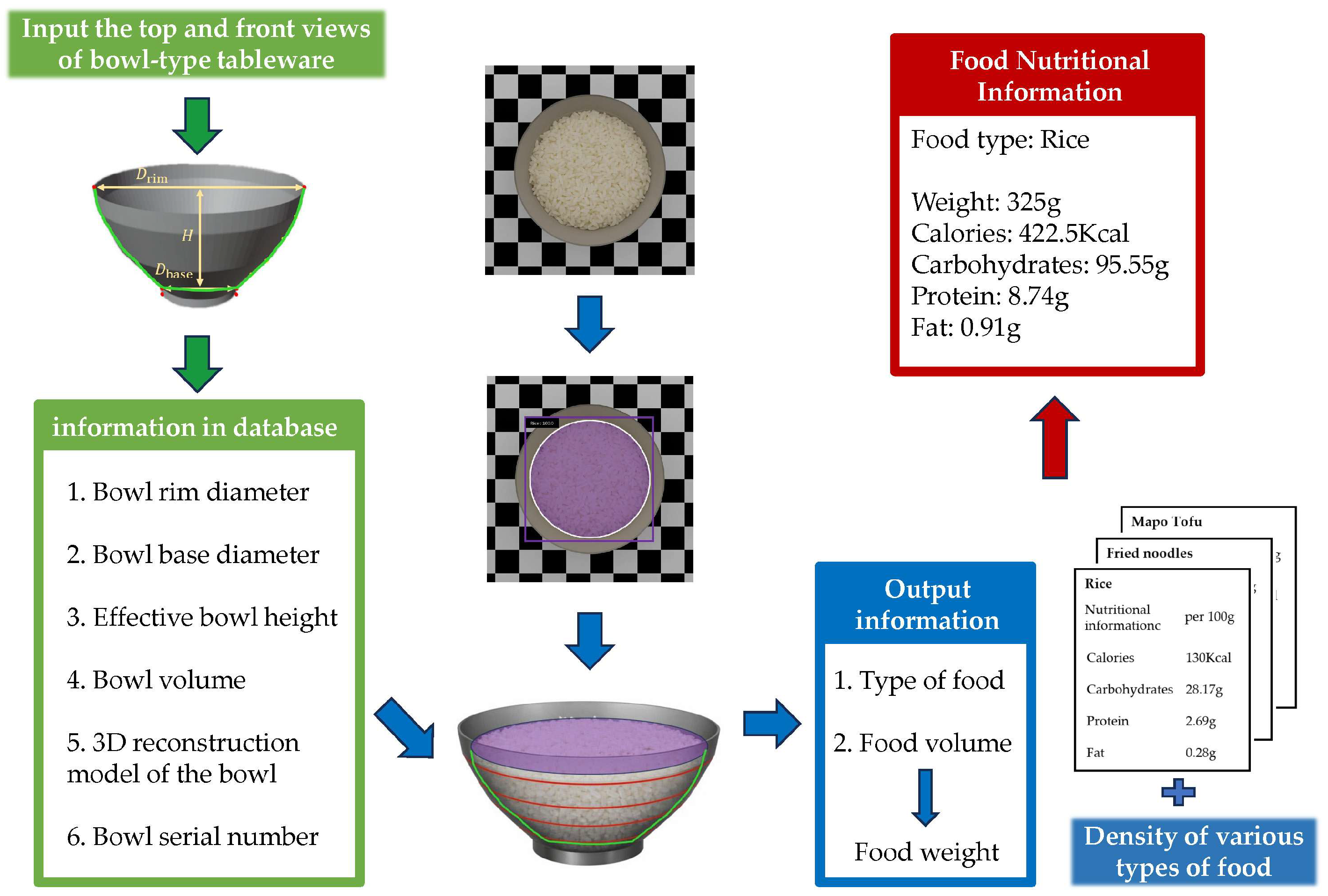
, this subsection further implements the prediction of the nutrient content of food contained in the bowl. We consider eight common food categories: Rice, Mapo Tofu, Kung Pao Chicken, Fried Noodles, Stir-fried Vegetables, Braised Eggplant, Tomato Scrambled Eggs, and Stir-fried Shredded Potatoes. To make predictions, food is placed in a bowl that has been registered in the database, and the food surface is kept as level as possible, without pronounced concavities or protrusions. In this study, only one type of food was placed in the nutritional composition experiment at a time to reduce the uncertainty caused by the combination of multiple foods. We then capture images under the same top-down setup as in the previous experiments, keeping the camera parameters and viewing angle unchanged, and perform instance mask segmentation on the food surface region. Unlike the single-class frontal-view segmentation of the “bowl” in
Section 2.5, this subsection requires simultaneous dish category recognition during segmentation. Therefore, the adopted mask segmentation network performs category classification alongside mask prediction.
Table 9 lists the eight food categories and the number of samples within different portion-size ranges, which are used to train and evaluate the model.
In the geometric estimation stage, the procedure is consistent with the liquid volume prediction in
Section 2.7.1. First, an equivalent circle radius (in pixel units) is obtained by fitting a circle to the segmented food surface in the top-down image, and the calibration factor is used to convert it to a physical-scale radius. Next, the corresponding height
is inferred from the inner-wall function
, and the food volume in the bowl,
is computed via axisymmetric integration. We then introduce the density parameter
for each food category and convert volume to weight as
. Finally, based on the per-unit-weight contents of calories, carbohydrates, protein, and fat for each dish, we compute the total nutrient amounts for the serving in the bowl, thereby completing nutrient content prediction.
Figure 14 presents the workflow for food nutrient content prediction.
2.7.3. Experimental Results and Analysis of Estimating the Relationship Between Liquid Volume and Food Nutrient Content
In this subsection, under the same experimental equipment and imaging conditions as in
Section 2.4.7 (with identical camera parameters, top-down viewing angle, resolution, and calibration factor), we evaluate the performance of different mask segmentation models on two tasks: liquid volume estimation in bowls and food volume estimation in bowls. In our dataset, there are 48 images of liquids in bowls, and the number of images for the eight food categories is as listed in
Table 2. We assign an ID to each image and record the corresponding liquid volume and food weight in a spreadsheet. Data augmentation is applied to both the liquid and food images, resulting in 144 augmented liquid images and 1929 augmented images in total for the eight food categories. We then train standard Mask R-CNN models for the two tasks separately. To ensure a fair comparison, both tasks use the same input preprocessing pipeline and the same training/test split strategy; the only difference lies in the category space. The liquid task is a single-class mask segmentation problem that distinguishes only liquid from background, whereas the food task is a multi-class instance segmentation problem that outputs both masks and category labels, with the category set consisting of the eight dishes listed in
Table 7.
During inference, the model first outputs the mask of the liquid or the visible food surface in the bowl, and the food task additionally outputs the predicted category. The mask is then processed by geometric circularization. Specifically, boundary points are extracted from the mask, and the OpenCV toolbox version 4.10.0 is used for contour extraction and circle fitting. Based on the extracted boundary point set, an equivalent circle is estimated using a least-squares strategy, yielding the pixel-scale radius of the fitted surface circle. This radius is converted to a physical radius using the pixel-to-world mapping factor . Because the bowl cavity is a solid of revolution formed by rotating the inner-wall profile about the central axis, a given surface radius corresponds to a unique height. Therefore, the height of the liquid level or food surface above the bowl bottom can be obtained by solving . Finally, given the upper height limit, we integrate using the axisymmetric volume formula to obtain the liquid volume or food volume in the bowl. For the food task, after volume estimation, the nutrient amounts are further quantified by combining the dish-specific density and the per-unit-mass nutrient table for each category.
We evaluate the mask segmentation quality of different models using COCO-style metrics, including the mean average precision for bounding-box detection () and the mean average precision for mask segmentation ().
In the bowl liquid-volume prediction experiment, we use the Mask R-CNN segmentation model to extract surface masks from the liquid images in the test set and predict liquid volume according to the aforementioned method. The predicted volumes are then compared with the recorded volumes in the spreadsheet to compute the prediction error. The liquid-surface mask segmentation performance and the liquid-volume prediction results are summarized in
Table 10. And
Table 11 shows a comparison of the average errors of different research methods in liquid volume prediction.
As shown in
Table 8, the mean prediction error for liquid volume estimation is 9.24%. We measured the density of each food category using a 200 mL measuring cup(Yancheng, Jiangsu, China), following the same filling procedure for all foods. To address the potential volume-to-weight conversion bias introduced by uneven food density and variations in packing tightness, this study conducted 20 repeated measurements for each food category during the density statistics phase. Density data was obtained under both lightly and tightly packed packing conditions, and the average value was taken to improve the robustness of density estimation. For nutritional data, priority was given to food composition data resources with more standardized and traceable sources, including Foundation Foods and SR Legacy categories from USDA FoodData Central, as well as the UK’s CoFID. Cross-checking across multiple databases was performed when necessary to reduce the impact of item matching bias and differences between single databases on the results. Related validation studies showed that Evenepoel et al. compared MyFitnessPal’s nutritional calculations with the research-grade Nubel food composition table, reporting errors of approximately 1.3% for energy and 1.2% for fat [
51]; Chiplonkar et al. compared food composition table estimates with laboratory chemical analysis results of cooked foods, indicating that the differences in protein and carbohydrate content were typically around 5% [
52]. Based on the experimental procedure described in this paper, the aforementioned differences mainly manifest as limited perturbations in nutrient values per unit weight. These perturbations are typically smaller than the error contributions introduced by volume estimation and density measurement, and represent a common external error source in the comparison of different methods. Therefore, their overall impact on the nutrient prediction conclusions is relatively limited. We obtained the nutrient information per 100 g for each dish, and
Table 12 summarizes the density and nutrient composition per unit weight for each food category.
In the food nutrient content prediction experiment, we likewise use a Mask R-CNN segmentation model to extract surface masks from the food images in the test set and estimate food volume according to the aforementioned procedure. The estimated volume is converted to food weight using the density of the corresponding food category, and the predicted weight is compared with the recorded weights in the spreadsheet to compute the prediction error. We then estimate the nutrient amounts by combining the predicted food weight with the per-100 g nutrient values in
Table 9. Therefore, the accuracy of nutrient content prediction is closely tied to the accuracy of the predicted food weight. Under this approach, the prediction error of food nutrient content is equivalent to the prediction error of food weight. The mask segmentation performance for different food categories and the weight prediction results are reported in
Table 13.
As shown in
Table 10, the mean weight prediction error for each food category ranges from 8.55% to 14.91%, and the overall mean weight prediction error across the eight food categories is 11.49%. Stir-fried Vegetables exhibits the largest weight prediction error. This is mainly because the density of a given dish is not a fixed constant and can vary substantially with cooking and serving conditions. Specifically, even within the same category, differences in oil usage, moisture content of sauces, and ingredient composition can directly change the solid content and porosity per unit volume. In addition, the stacking pattern and degree of compaction during filling affect the actual volume distribution and effective density of the food in the bowl, which in turn leads to larger deviations in weight prediction.
Table 14 compares the average errors of different research methods in predicting the content of food nutrients.
2.7.4. Visual User Platform
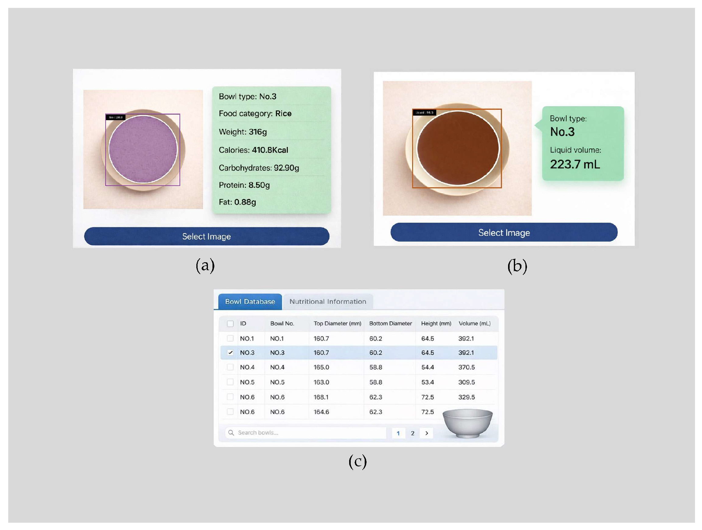
Based on the above analysis pipeline, we developed a visualization and user-facing platform, as shown in
Figure 15. After a one-time camera calibration, the user only needs to provide a frontal-view and a top-down image of a bowl. The system can then automatically identify geometric parameters such as the rim diameter, base diameter, effective height, and the inner-wall contour curve, and store the recognized results and the reconstructed model as a bowl instance in the database. For liquid volume and food nutrient content prediction, the user selects the bowl type and inputs a top-down image of the liquid or food in the bowl, and the platform outputs the predicted liquid volume or the food category together with its estimated nutrient content.
The platform can be applied to standardized portioning and output management in food retail, dietary intake monitoring in hospitals or elderly-care settings, calorie logging for fitness and weight management, as well as quantitative liquid dispensing and container capacity assessment under laboratory conditions. Looking ahead, the system can be extended to more vessel types and more complex food geometries, and multi-view or depth cues can be incorporated to improve robustness to uneven surfaces and occlusions. In addition, developing finer-grained prediction modules and providing AI-driven dietary recommendations could further enhance the generalization capability and interpretability of the nutritional assessment.