Next Article in Journal
Scheduling Intrees with Unavailability Constraints on Two Parallel Machines
Next Article in Special Issue
Confidence Intervals for the Difference and Ratio Means of Zero-Inflated Two-Parameter Rayleigh Distribution
Previous Article in Journal
Waiting Time in an MSP Queue with Active Management
Previous Article in Special Issue
Symmetric Discrete Distributions on the Integer Line: A Versatile Family and Applications
error_outline You can access the new MDPI.com website here. Explore and share your feedback with us.
 
 
Article

Statistical Estimation of Common Percentile in Birnbaum–Saunders Distributions: Insights from PM2.5 Data in Thailand

1
Department of Statistics, Faculty of Science, Ramkhamhaeng University, Bangkok 10240, Thailand
2
Department of Applied Statistics, Faculty of Applied Science, King Mongkut’s University of Technology North Bangkok, Bangkok 10800, Thailand
3
Department of Data Science and Application, School of Information and Communication Technology, University of Phayao, Phayao 56000, Thailand
*
Author to whom correspondence should be addressed.
Symmetry 2026, 18(1), 100; https://doi.org/10.3390/sym18010100
Submission received: 24 November 2025 / Revised: 2 January 2026 / Accepted: 4 January 2026 / Published: 6 January 2026

Abstract

This study develops approaches for estimating the common percentile of Birnbaum–Saunders (BS) distributions and applies them to daily PM2.5 concentration data from six monitoring stations in Chiang Mai Province, Thailand. Percentiles provide a robust representation of typical pollutant exposure, being less sensitive to outliers and suitable for skewed environmental data. Estimating the same percentile across multiple monitoring sites offers a standardized metric for regional air quality assessment, enabling meaningful comparisons and informing evidence-based environmental policy. Four statistical approaches—Generalized Confidence Interval (GCI), bootstrap, Bayesian, and Highest Posterior Density (HPD)—were employed to construct confidence intervals (CIs) for the common percentile. Simulation studies evaluated the methods in terms of average length (AL) and coverage probability (CP), showing that the GCI approach offers the best balance between precision and reliability. Application to real PM2.5 data confirmed that the BS distribution appropriately models pollutant concentrations and that the common percentile provides a meaningful measure for environmental assessment. These findings highlight the GCI method as a robust tool for constructing CIs in environmental data analysis.

1. Introduction

Percentiles based on the Birnbaum–Saunders (BS) distribution offer notable benefits for statistical inference, particularly for positively skewed and nonnegative data commonly encountered in lifetime analysis, reliability engineering, and environmental studies. Relative to moment-based summaries, BS percentiles are more resistant to the influence of extreme observations and provide meaningful interpretation at specified risk or exposure levels. One key advantage of the BS framework is that its percentile function is available in closed form, enabling efficient computation, facilitating bootstrap and resampling-based inference, and allowing confidence intervals to be obtained without numerical inversion. Moreover, BS percentiles effectively describe upper-tail behavior arising from fatigue and cumulative damage mechanisms, making them especially appropriate for inference on high-order quantiles that are often of primary practical interest. Overall, these features establish BS percentiles as a flexible and computationally efficient alternative to mean-based or purely empirical quantile methods when the focus lies on tail-related characteristics.
Extensive research has addressed statistical inference for percentiles. Marshall and Walsh [1] were among the first to compare percentage points from two continuous populations. Harrell and Davis [2] introduced a quantile estimator, and Kaigh and Lachenbruch [3] later offered a different estimation method. Albers and Löhnberg [4] proposed distribution-free confidence intervals (CIs) for quantile differences in biomedical studies. Cox and Jaber [5] explored tests for the equality of percentiles in normal distributions. Chang and Tang [6] constructed CIs for BS percentiles, while Padgett and Tomlinson [7] derived lower confidence bounds for percentiles from Weibull and BS distributions. Guo and Krishnamoorthy [8] developed Generalized Confidence Intervals (GCIs) and p-values to compare quantiles of two normal populations. Huang and Johnson [9] focused on inference regarding the ratio of two normal percentiles. More recent work includes Navruz and Özdemir [10], who introduced a bootstrap approach for comparing percentiles between independent groups, and Hasan and Krishnamoorthy [11], who constructed CIs for the mean and upper percentiles of nonnegative log-normal data. Abdollahnezhad and Jafari [12] additionally proposed a small-sample adjustment to the likelihood ratio test for assessing quantile equality across several normal populations.
Fine particulate matter (PM2.5) is a major component of air pollution and remains a serious challenge to both environmental sustainability and human health. High concentrations of PM2.5 are commonly observed in various parts of the world, including northern Thailand, where levels often surpass international safety standards and pose significant public health risks. Tackling this issue effectively depends on reliable environmental monitoring and the use of sophisticated data analysis techniques to uncover pollution trends and guide policy decisions. PM2.5 consists of very fine airborne particles with diameters under 2.5 micrometers. Because of their tiny size, they can penetrate deep into the lungs and even enter the bloodstream, leading to significant health hazards. Prolonged or high-level exposure has been associated with respiratory and cardiovascular diseases, as well as increased mortality. Key sources of PM2.5 include emissions from vehicles, industrial activities, biomass burning, and natural events such as wildfires and dust storms. Urban centers and rapidly developing regions are particularly at risk due to high population density and concentrated human activity. In northern Thailand, PM2.5 concentrations regularly exceed the limits set by the World Health Organization (WHO), intensifying concerns about environmental health and long-term sustainability. Consequently, monitoring PM2.5 levels and understanding their patterns is essential for evaluating environmental and health effects. Sophisticated statistical analysis is essential for detecting patterns, predicting pollution spikes, and developing effective mitigation strategies. Because PM2.5 data are often skewed due to sporadic but severe pollution events, traditional summary measures like the mean may not accurately capture typical exposure levels. In contrast, percentiles offer a more robust and representative measure, making them an increasingly important tool in evidence-based air quality management and policy formulation. Daily PM2.5 concentrations from six monitoring stations in Chiang Mai Province, Thailand, were analyzed due to their non-negative and positively skewed distribution, characteristics well captured by the BS model. The BS distribution is particularly suitable for environmental pollutants like PM2.5, which can exhibit extreme values during episodic pollution events. Chiang Mai’s pronounced seasonal air quality variability, especially during the biomass-burning period, provides an ideal context to demonstrate the robustness of the BS distribution and the estimation of common percentiles across multiple monitoring sites.
This study emphasizes the application of the BS distribution, a flexible statistical model specifically suited for positively skewed data, to analyze PM2.5 concentrations. The suitability of this distribution lies in its ability to accurately capture the asymmetry in pollutant levels arising from irregular but severe pollution episodes, such as seasonal biomass burning or industrial emissions. By estimating a common percentile across multiple monitoring stations, the study introduces a unified and consistent metric for regional air quality assessment (Chang and Tang [6] and Padgett and Tomlinson [7]). This approach not only simplifies comparative analysis across different locations but also enhances the reliability of environmental evaluations. A common percentile serves as a central measure of air pollution levels, facilitating data-driven decisions for public health management and environmental policy formulation. Furthermore, using percentiles within the BS modeling framework helps quantify typical exposure levels more effectively than traditional methods (Harrell and Davis [2] and Guo and Krishnamoorthy [8]). This is particularly valuable for stakeholders and decision-makers who must prioritize resources, design mitigation strategies, and set regulatory standards based on realistic and population-relevant exposure metrics. In summary, percentile-based analysis, supported by the BS distribution, provides a meaningful and statistically sound approach for assessing PM2.5 pollution. It enables a comprehensive and harmonized understanding of air quality across regions, ultimately contributing to more effective environmental monitoring and public health protection. There has been substantial scholarly attention devoted to statistical inference for the parameters of the BS distribution. Guo et al. [13] investigated inference procedures for estimating a common mean across multiple BS populations. Shakil et al. [14] conducted a comprehensive study of inference methods for the three-parameter BS distribution, highlighting its statistical properties, theoretical characterizations, and practical applications. More recently, Thangjai et al. [15] developed a GCI approach for comparing percentiles of BS distributions, with an application to PM2.5 concentrations in Thailand. Earlier work by Leiva et al. [16] extended the BS model to a generalized form suitable for modeling pollution data, including both positive and negative moments. Wang [17] further contributed by proposing generalized interval estimation techniques for the BS distribution. Additionally, Niu et al. [18] compared two hypothesis testing methods for BS parameters—one employing the exact generalized p-value approach and the other relying on the Delta method—highlighting their relative performance.
A common percentile represents the same relative position across multiple distributions. When data are collected from different monitoring stations, each site may have its own distribution, but the common percentile approach assumes that a fixed percentile level (e.g., the 75th) is shared across all locations, even if the corresponding concentration values differ. This provides a unified and interpretable measure of typical exposure that supports meaningful comparisons while accounting for local variability. Evaluating uncertainty around common percentiles is essential for reliable environmental assessments and informed policy decisions. This study explores four statistical approaches for constructing CIs: GCI, bootstrap, Bayesian, and Highest Posterior Density (HPD). These methods are all implemented using R software (version 2024.12.0+467), a popular tool for statistical analysis and data processing. Although frequently used to estimate parameters such as means and variances, these techniques are less commonly applied to percentiles, despite the critical role percentiles play in environmental studies where data distributions are often skewed by occasional extreme pollution events. The versatility of R software (version 2024.12.0+467) facilitates the effective application of these techniques: bootstrap methods rely on resampling to empirically build CIs; Bayesian and HPD approaches use Markov Chain Monte Carlo (MCMC) simulations to approximate posterior distributions; and GCI approach involves programming generalized pivotal quantities (GPQs) for interval estimation. By comparing these R-based methods for estimating CIs of percentiles, the study offers valuable insights into their comparative benefits and practical uses. This knowledge aids researchers and policymakers in choosing robust statistical tools that enhance the precision of air quality assessments, improve uncertainty estimation, and support better environmental decision-making. The study evaluates the performance of each method through simulation experiments, considering criteria such as average length (AL) and coverage probability (CP). Subsequently, the methods are applied to actual daily PM2.5 data collected from six monitoring stations in Chiang Mai Province, Thailand. The findings underscore the practical effectiveness of each approach and contribute to the advancement of reliable techniques for environmental data analysis and policy development.

2. Common Percentile

Let X i j be a random variable that follows a BS distributions with shape parameter α i and scale parameter β i , where i = 1 , 2 , , k and j = 1 , 2 , , n i . According to Thangjai et al. [15], the percentile of X i j is
θ i = β i 4 α i z p + α i 2 z p 2 + 4 2 ,
where z p = Φ 1 ( p ) is the p-th quantile of the standard normal distribution.
The estimator of β i is defined as
β ^ i = { max ( β ^ 1 i , β ^ 2 i ) ; T i 0 min ( β ^ 1 i , β ^ 2 i ) ; T i > 0 ,
where β ^ 1 i and β ^ 2 i are two solutions of β ^ i . The value of β ^ i can be obtained by solving
A i β ^ i 2 2 B i β ^ i + C i = 0 ,
where A i = n i 1 J i 2 1 n i L i T i 2 , B i = n i 1 I i J i ( 1 I i J i ) T i 2 , C i = n i 1 I i 2 1 n i K i T i 2 , I i = 1 n i j = 1 n i X i j , J i = 1 n i j = 1 n i 1 X i j , K i = j = 1 n i X i j I i 2 , L i = j = 1 n i 1 X i j J i 2 and T i t n i 1 is t-distribution with n i 1 degrees of freedom.
The variance of β ^ i is
V a r β ^ i = α i 2 β i 2 n i 1 + 3 4 α i 2 1 + 1 2 α i 2 2 .
The estimator of α i is defined as
α ^ i = β ^ i 2 j = 1 n i 1 X i j 2 n i β ^ i + j = 1 n i X i j β ^ i V i ,
where V i χ 2 n i is the chi-squared distribution with n i degrees of freedom.
The variance of α ^ i is
V a r α ^ i = α i 2 2 n i .
The estimator of θ i is
θ ^ i = β ^ i 4 α ^ i z p + α ^ i 2 z p 2 + 4 2 .
From Appendix A, the variance of θ ^ i is
V a r θ ^ i = α i 2 β i 2 8 n i α i z p + α i 2 z p 2 + 4 2 z p + α i z p 2 α i 2 z p 2 + 4 2 + 4 + 3 α i 2 2 2 + α i 2 2 α i z p + α i 2 z p 2 + 4 2 .
The estimate of the variance of θ ^ i is
V a r ^ θ ^ i α ^ i 2 β ^ i 2 8 n i α ^ i z p + α ^ i 2 z p 2 + 4 2 z p + α ^ i z p 2 α ^ i 2 z p 2 + 4 2 + 4 + 3 α ^ i 2 2 2 + α ^ i 2 2 α ^ i z p + α ^ i 2 z p 2 + 4 2 .
The common percentile θ ^ is calculated as the weighted average of θ ^ i across the k individual sample. It is defined as
θ ^ = i = 1 k θ ^ i V a r ^ θ ^ i / i = 1 k 1 V a r ^ θ ^ i .

2.1. Generalized Confidence Interval Approach

A GCI is a statistical method designed to create CIs in complex or non-standard situations where conventional approaches either fail or are unsuitable. This modern and versatile technique is especially valuable when traditional CI methods fall short. GCIs utilize simulations and the concept of GPQs to produce reliable intervals in challenging inference problems. Traditional CIs typically depend on well-understood sampling distributions, such as the sample mean following a normal distribution, as justified by the Central Limit Theorem. However, in many practical situations, the sampling distribution might be unknown or too complicated to derive, or the estimator may involve nuisance parameters, which are variables that are not of primary interest but still influence the distribution. Additionally, the parameter being estimated may be a complex function of multiple random variables. To overcome these difficulties, the GCI method constructs a GPQ, which is a random variable that depends on both the observed data and a simulated random variable with a known distribution. When the sample data is plugged in, the GPQ becomes free of any unknown parameters. By simulating the distribution of the GPQ and using its empirical percentiles, one can determine confidence bounds corresponding to a desired confidence level.
The GPQ for θ i is constructed using the GPQs of β i and α i . According to Sun [19], the GPQ of β i is
R β i = { max ( β 1 i , β 2 i ) ; T i 0 min ( β 1 i , β 2 i ) ; T i > 0 ,
where β 1 i and β 2 i are two solutions for β i .
According to Wang [17], the GPQ of α i is
R α i = R β i 2 j = 1 n i 1 X i j 2 n i R β i + j = 1 n i X i j R β i V i .
The GPQ for θ i is
R θ i = R β i 4 R α i z p + R α i 2 z p 2 + 4 2 .
The estimate of variance of R θ i is
R V a r θ ^ i R α i 2 R β i 2 8 n i R α i z p + R α i 2 z p 2 + 4 2 z p + R α i z p 2 R α i 2 z p 2 + 4 2 + 4 + 3 R α i 2 2 2 + R α i 2 2 R α i z p + R α i 2 z p 2 + 4 2 ,
where z p = Φ 1 ( p ) is the p-th quantile of the standard normal distribution and R β i is defined in Equation (11), and R α i is defined in Equation (12).
The GPQ for the common percentile is
R θ = i = 1 k R θ i R V a r θ ^ i / i = 1 k 1 R V a r θ ^ i .
Therefore, the 100 1 γ % two-sided GCI is
C I G C I = L G C I , U G C I = R θ γ / 2 , R θ 1 γ / 2 ,
where R θ γ / 2 and R θ 1 γ / 2 denote the 100 γ / 2 -th and 100 1 γ / 2 -th percentiles of R θ , respectively. Algorithm 1 was used to construct the GCI.
Algorithm 1 GCI
  • Step 1: Compute A i , B i , and C i
  • Step 2: At the m step
  • (a) Simulate T i t ( n i 1 ) and compute R β i . If R β i < 0 , resimulate T i t ( n i 1 )
  • (b) Simulate V i χ 2 ( n i ) and compute R α i , R θ i , R V a r θ ^ i , and R θ
  • Step 3: Repeat step 2 a total of M times to obtain an array of R θ values
  • Step 4: Compute L G C I and U G C I

2.2. Bootstrap Approach

A bootstrap CI is a statistical technique used to estimate the range in which a population parameter is likely to lie, based solely on sample data. It is particularly useful when the underlying distribution of the data is unknown or too complex to model analytically. This method involves repeatedly resampling the original dataset with replacement. It is also effective for estimating CIs for complex statistics where traditional methods may be inadequate.
Let x i j be a random sample drawn from BS distributions with parameters α i and β i , where i = 1 , 2 , , k and j = 1 , 2 , , n i . Let x i j * be a bootstrap sample drawn from BS distributions with parameters α ^ i and β ^ i , where i = 1 , 2 , , k , j = 1 , 2 , , n i and α ^ i and β ^ i are the maximum likelihood estimators of α i and β i , respectively. Then, the α ^ i * and β ^ i * are obtained using B bootstrap samples. The respective correct estimates for α ^ i * and β ^ i * are
α ˜ i ( r ) = α ^ i ( r ) * 2 b ^ α ^ i , α i
and
β ˜ i ( r ) = β ^ i ( r ) * 2 b ^ β ^ i , β i ,
where b ^ α ^ i , α = 1 B r = 1 B α ^ i ( r ) * α ^ i , b ^ β ^ i , β = 1 B r = 1 B β ^ i ( r ) * β ^ i , and r = 1 , 2 , , B .
The bootstrap estimator of θ i is
θ ^ i ( r ) = β ˜ i ( r ) 4 α ˜ i ( r ) z p + α ˜ i ( r ) 2 z p 2 + 4 2 .
The bootstrap estimator of the variance of θ ^ i ( r ) is
V a r ^ θ ^ i ( r ) α ˜ i ( r ) 2 β ˜ i ( r ) 2 8 n i α ˜ i ( r ) z p + α ˜ i ( r ) 2 z p 2 + 4 2 z p + α ˜ i ( r ) z p 2 α ˜ i ( r ) 2 z p 2 + 4 2 + 4 + 3 α ˜ i ( r ) 2 2 2 + α ˜ i ( r ) 2 2 α ˜ i ( r ) z p + α ˜ i ( r ) 2 z p 2 + 4 2 .
The bootstrap estimator of the common percentile is
θ ^ r = i = 1 k θ ^ i ( r ) V a r ^ θ ^ i ( r ) / i = 1 k 1 V a r ^ θ ^ i ( r ) .
Therefore, the 100 1 γ % two-sided bootstrap CI is
C I B C I = L B C I , U B C I = θ ^ r γ / 2 , θ ^ r 1 γ / 2 ,
where θ ^ r γ / 2 and θ ^ r 1 γ / 2 denote the 100 γ / 2 -th and 100 1 γ / 2 -th percentiles of θ ^ r , respectively. Algorithm 2 was used to construct the bootstrap CI.
Algorithm 2 Bootstrap CI
  • Step 1: Specify the values of x i j
  • Step 2: At the b step
  • (a) Generate x i j *
  • (b) Compute α ˜ i ( r ) , β ˜ i ( r ) , θ ^ i ( r ) , V a r ^ θ ^ i ( r ) , and θ ^ r
  • Step 3: Repeat step 2 a total of B times to obtain an array of θ ^ r values
  • Step 4: Compute L B C I and U B C I

2.3. Bayesian Approach

The Bayesian approach is a statistical inference method that views probability as a reflection of belief or confidence, rather than relying solely on long-run frequencies. It is based on Bayes’ Theorem, which provides a way to revise the likelihood of a hypothesis as new data or evidence becomes available. A prior reflects existing knowledge or assumptions about the parameters or model before any data is observed. Priors may be informative, drawing from previous research, or non-informative, implying little to no prior knowledge. The likelihood expresses the probability of the observed data given various parameter values. The posterior represents the updated belief after incorporating the data, which is the central aim of Bayesian inference: to determine the posterior distribution of the model parameters or hypotheses. Key benefits of the Bayesian approach include its ability to incorporate prior information, its production of full probability distributions, and its flexibility in complex modeling scenarios.
The Bayesian approach offers a systematic way to include prior knowledge and adjust beliefs as new data becomes available. This is particularly useful in complex models where parameters are supported by theoretical insights or empirical evidence. Within this framework, the posterior distribution is derived using Bayes’ Theorem, allowing the model to be updated progressively as more information is gathered.
In the study by Wang et al. [20], inverse gamma distributions were used as prior distributions for the parameters β i and α i 2 . Suppose that β i follows an inverse gamma distribution with parameters a i 1 and b i 1 , denoted as I G β i | a i 1 , b i 1 . Similarly, suppose that α i 2 follows an inverse gamma distribution with parameters a i 2 and b i 2 , denoted as I G α i 2 | a i 2 , b i 2 . The marginal distribution of β i is
p ( β i | x i ) β i ( n i + a i 1 + 1 ) exp b i 1 β i j = 1 n i β i x i j 1 2 + β i x i j 3 2 j = 1 n i 1 2 x i j β i + β i x i j 2 + b i 2 n i + 1 2 a i 2 .
The conditional posterior distribution of α i 2 given β i is expressed as
p ( α i 2 | x i , β i ) I G n i 2 + a i 2 , 1 2 j = 1 n i x i j β i + β i x i j 2 + b i 2 .
The samples shown in Equations (23) and (24) are generated using MCMC methods, a common approach in Bayesian analysis for estimating complex posterior distributions. MCMC algorithms produce a sequence of dependent samples that, under appropriate conditions, converge to the desired posterior distribution. These methods are especially useful when analytical solutions are difficult or impossible to obtain, such as in models with high dimensionality or non-standard probability structures.
Wang et al. [20] utilized the generalized ratio-of-uniforms technique to generate posterior samples for the parameter β i . This technique was originally introduced by Wakefield et al. [21]. This technique relies on constructing a pair of random variables u i , v i , each drawn from a uniform distribution over a specifically defined region. That is,
A ( r i ) = ( u i , v i ) : 0 < u i p v i u i r i | x i 1 r i + 1 , r i 0 ,
where r i is a constant and p · | x i is defined according to Equation (23). As a result, the variable β i = v i u i r i has a probability density proportional to p ( β i | x i ) p ( β i | x i ) d β i . To generate random samples from the region A ( r i ) , the variables u i , v i are drawn uniformly from a one-dimensional bounded rectangle that encloses the region [ 0 , a ( r i ) ] × [ b ( r i ) , b + ( r i ) ] , where a ( r i ) = sup β i > 0 [ p ( β i | x i ) ] 1 r i + 1 , b ( r ) = inf β i > 0 β i [ p ( β i | x i ) ] r i r i + 1 , and b + ( r i ) = sup β i > 0 β i [ p ( β i | x i ) ] r i r i + 1 .
Wang et al. [20] assumed that a ( r i ) and b + ( r i ) are finite and that the condition b ( r i ) = 0 holds. A proposed variate β i = v i u i r i is accepted if u i [ p ( β i | x i ) ] 1 r i + 1 it satisfies this condition; otherwise, the sampling procedure is repeated. Posterior samples for the parameter α i 2 are obtained using the LearnBayes package in the R programming environment. Consequently, the square root of the sampled values α i 2 corresponds to the posterior samples of the target parameter α i .
The posterior distribution of θ i is
θ i . B a y e = β i 4 α i z p + α i 2 z p 2 + 4 2 .
The estimator of the variance of θ i . B a y e is
V a r ^ θ i . B a y e α i 2 β i 2 8 n i α i z p + α i 2 z p 2 + 4 2 z p + α i z p 2 α i 2 z p 2 + 4 2 + 4 + 3 α i 2 2 2 + α i 2 2 α i z p + α i 2 z p 2 + 4 2 .
The Bayesian estimator of the common percentile is
θ B a y e = i = 1 k θ i . B a y e V a r ^ θ i . B a y e / i = 1 k 1 V a r ^ θ i . B a y e .
Therefore, the 100 1 γ % two-sided Bayesian credible interval is
C I B a y e = L B a y e , U B a y e = θ B a y e γ / 2 , θ B a y e 1 γ / 2 ,
where θ B a y e γ / 2 and θ B a y e 1 γ / 2 denote the 100 γ / 2 -th and 100 1 γ / 2 -th percentiles of θ B a y e , respectively. Algorithm 3 was used to construct the Bayesian credible interval.
Algorithm 3 Bayesian credible interval and HPD interval
  • Step 1: Specify the values of a i 1 , a i 2 , b i 1 , b i 2 , and r i , then compute a ( r i ) and b + ( r i )
  • Step 2: At the m step
  • (a) Generate u i and v i
  • (b) Compute ρ i = v i u i r i
  • (c) If the value of ρ i is accepted, set β i ( m ) = ρ i if u i [ p ( β i | x i ) ] 1 r i + 1 ; otherwise, repeat step (a) and step (b)
  • (d) Generate α i 2 and compute α i ( m ) = α i 2
  • (e) Compute θ i , V a r ^ θ i . B a y e , and θ B a y e
  • Step 3: Repeat step 2 a total M times to obtain an array of θ B a y e values
  • Step 4: Compute L B a y e and U B a y e
  • Step 5: Compute L H P D and U H P D

2.4. Highest Posterior Density Approach

The HPD approach is a technique in Bayesian statistics used to define credible intervals (also known as Bayesian credible intervals) for estimating unknown parameters. In contrast to traditional CIs, which rely on the concept of repeated sampling, HPD intervals are directly obtained from the posterior distribution of the parameter. An HPD interval represents the smallest possible range that contains a given proportion (such as 95%) of the total posterior probability. Simply put, it identifies the most plausible range of values for the parameter, based on both the observed data and prior knowledge. In this way, the HPD interval highlights the values with the highest probability density under the posterior distribution.
The HPD interval was derived from the posterior distribution described in Equation (28). Among all intervals that include 100 1 γ % of the posterior probability, it has the shortest length. Every value inside the interval has a higher posterior density than any value outside it.
Therefore, the 100 1 γ % two-sided HPD interval is
C I H P D = L H P D , U H P D ,
where L H P D and U H P D are obtained using the hdi function from the HDInterval package in the R software (version 2024.12.0+467) environment. Algorithm 3 was used to construct the HPD interval.

3. Results

This study investigates various techniques for constructing CIs, including the GCI, bootstrap, Bayesian, and HPD approaches. The effectiveness of these approaches was evaluated through a Monte Carlo simulation implemented in R software (version 2024.12.0+467). The simulation aimed to assess interval estimates for the common percentile of the BS distribution. Two primary performance indicators were used in the analysis: CP and AL. CP reflects the frequency with which the interval captures the true parameter value, whereas AL serves as a measure of precision, with shorter intervals indicating greater accuracy. A CI is considered optimal if it achieves a CP of at least 0.95 and simultaneously maintains the shortest possible AL. Through this comparative analysis, the study provides valuable insights into the reliability and efficiency of each method, aiding in the selection of the most appropriate technique for estimating intervals within the BS distribution framework.
To evaluate the effectiveness of the proposed CIs, Monte Carlo simulations were carried out using R software (version 2024.12.0+467) under various conditions, including different sample sizes ( n i ) and shape parameters ( α i ). The scale parameter ( β i ) was fixed at 1.00 across all simulation scenarios to maintain consistency. The simulation study consisted of 5000 Monte Carlo replications. In each replication, 1000 resampling iterations were conducted for each of the GCI, bootstrap, Bayesian, and HPD approaches. The performance of each method was assessed based on two key metrics: CP, defined as the proportion of times the true parameter value was captured within the CI, and AL, which reflects the precision of the interval, with shorter lengths indicating more accurate estimates. An ideal method is expected to achieve a CP equal to or exceeding the nominal confidence level of 0.95, while also minimizing the AL. The detailed computational procedure for estimating CPs and ALs for all approaches is outlined in Algorithm 4.
Algorithm 4 CPs and ALs
  • Step 1: Specify the values of n i , α i , β i , and θ
  • Step 2: Generate a sample x i j from the BS distributions
  • Step 3: Compute θ ^ i , V a r ^ θ ^ i , and θ ^
  • Step 4: Apply Algorithm 1 to construct [ L G C I ( m ) , U G C I ( m ) ]
  • Step 5: Apply Algorithm 2 to construct [ L B C I ( m ) , U B C I ( m ) ]
  • Step 6: Apply Algorithm 3 to construct [ L B a y e ( m ) , U B a y e ( m ) ] and [ L H P D ( m ) , U H P D ( m ) ]
  • Step 7: If L ( m ) θ U ( m ) , set p ( m ) = 1 else set p ( m ) = 0
  • Step 8: Compute U ( m ) L ( m )
  • Step 9: Repeat step 2–step 8, a total M times
  • Step 10: Compute the CPs as the mean of p ( m )
  • Step 11: Compute the ALs as the mean of U ( m ) L ( m )
Table 1 and Table 2 report the empirical CP and AL of four methods for constructing 95% CIs for a common percentile, evaluated through simulations under different combinations of sample sizes and parameters. For the three-sample cases, the sample size tuples ( n 1 , n 2 , n 3 ) represent the sizes of three independent samples drawn from BS distributions, with the shape parameters shown in parentheses ( α 1 , α 2 , α 3 ). Based on the results presented in Table 1 and Table 2, the GCI consistently has the longest ALs; however, its CPs are generally close to the nominal confidence level of 0.95 across most scenarios. In contrast, the bootstrap CI yields the shortest ALs, but its CPs fall below the nominal level of 0.95 in all cases, making it unsuitable for constructing CIs for a common percentile. The Bayesian credible interval achieves CPs near 0.95 in some scenarios, and its AL tends to be shorter than that of the GCI when both maintain similar coverage levels. However, the HPD interval consistently shows CPs below 0.95. Therefore, the GCI approach is recommended for constructing CIs for a common percentile in all cases, while the Bayesian approach becomes more suitable as sample sizes increase.

4. An Empirical Application

This section focuses on illustrating the proposed inferential framework using real PM2.5 data rather than on predictive time-series modeling. Although the observations are recorded sequentially over time, the analysis treats the data as realizations from underlying distributions to support inference on common percentiles across monitoring stations.
PM2.5 denotes fine particles with a diameter of 2.5 micrometers or smaller. Due to their tiny size, they can reach deep into the lungs and potentially enter the bloodstream, posing significant health hazards. Percentiles are statistical tools used to illustrate the variation in PM2.5 levels over time. For example, the 50th percentile, or median, indicates the value below which half of the PM2.5 readings fall. Likewise, the 95th percentile shows that 95% of the values are below a certain level, while the remaining 5% exceed it. Compared to simple averages, percentiles provide more detailed insight into pollution trends. They are particularly valuable in environmental and public health research, especially for detecting periods of high pollution. Using percentiles enables researchers and policymakers to monitor changes in air quality, identify extreme pollution events, and compare pollution levels across different regions and time periods. Therefore, percentile-based analysis of PM2.5 offers a more accurate and comprehensive understanding of air quality and its impact on human health and the environment.
Table 3 presents PM2.5 levels recorded at six monitoring stations in Chiang Mai Province between 1 January and 30 April 2025, as reported by the Pollution Control Department (http://air4thai.pcd.go.th/webV3/#/History, accessed on 1 November 2025). The stations are located in the following areas: Station 1—Chang Phueak Subdistrict, Mueang Chiang Mai District; Station 2—Si Phum Subdistrict, Mueang Chiang Mai District; Station 3—Suthep Subdistrict, Mueang Chiang Mai District; Station 4—Chang Khoeng Subdistrict, Mae Chaem District; Station 5—Mueang Na Subdistrict, Chiang Dao District; and Station 6—Hang Dong Subdistrict, Hot District. The PM2.5 measurements considered in this study are obtained from secondary data sources. Despite the presence of an N/A category denoting unavailable data, a detailed review of the dataset confirmed the absence of such entries throughout the study period, eliminating the need for any imputation or data correction procedures.
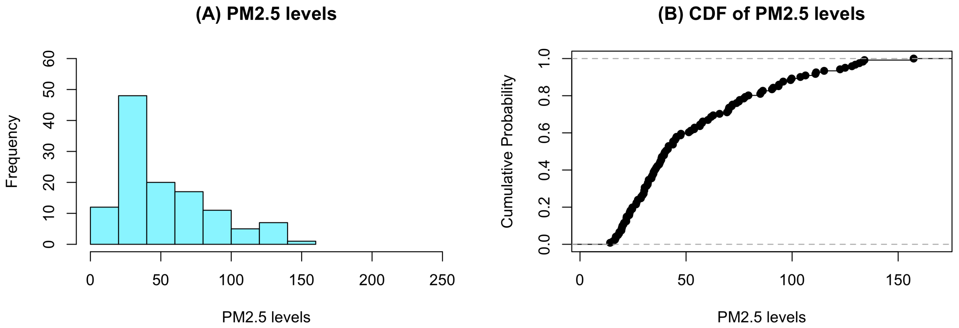
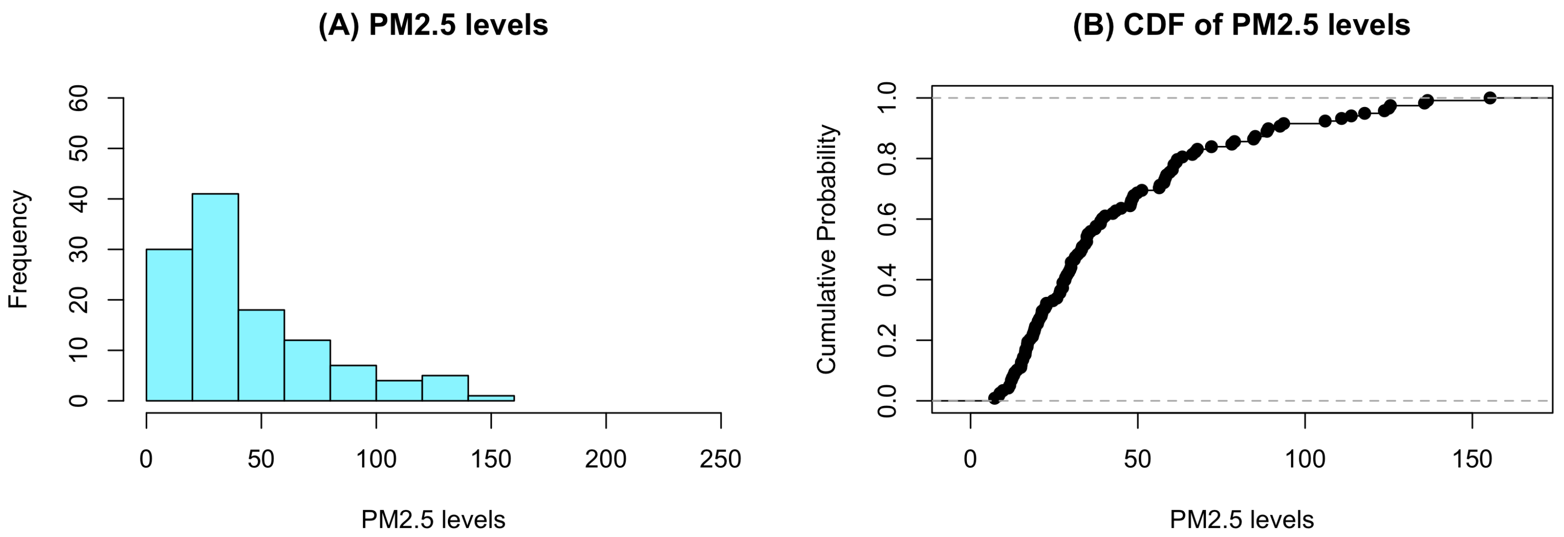
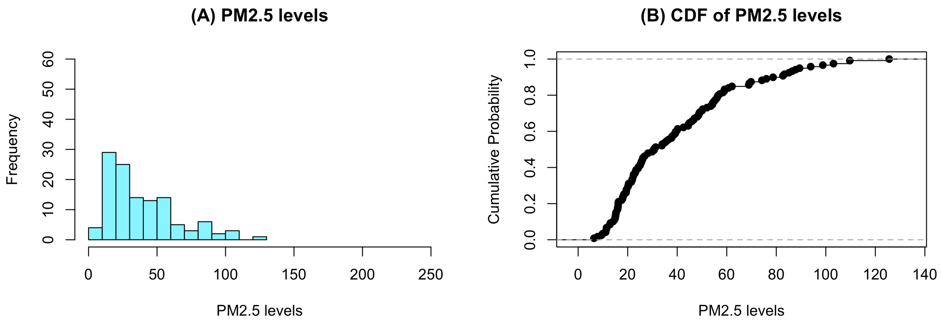
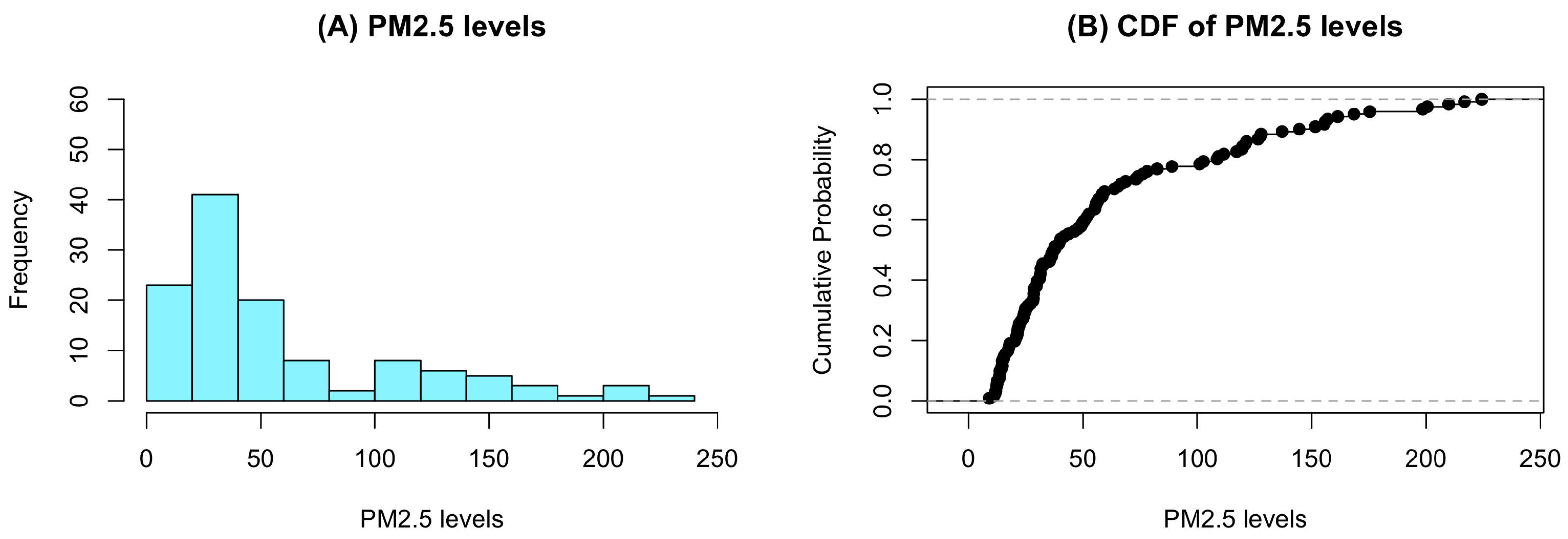
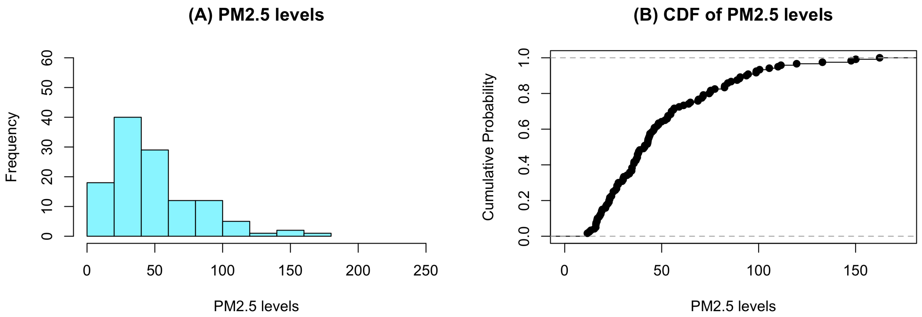
Figure 1, Figure 2, Figure 3, Figure 4, Figure 5 and Figure 6 show histograms illustrating the distribution of daily PM2.5 level data collected from six monitoring stations in Chiang Mai Province. These figures reveal that the data exhibit positively skewed distributions across all stations. The time-series plots and histograms are presented to describe the empirical characteristics of the PM2.5 data and to motivate the distributional assumptions, not to model temporal dependence or forecast future concentrations. Since the proposed analysis does not model temporal dependence or perform forecasting, stationarity assumptions and related tests are not required. Table 4 presents the estimated Akaike Information Criterion (AIC) values for various probability models fitted to the daily PM2.5 level data, including the normal, log-normal, Weibull, gamma, exponential, logistic, Cauchy, and BS distributions. The results indicate that, for all six stations, the BS distribution yields the lowest AIC values. This suggests that the BS distribution is the most suitable model for representing the daily PM2.5 level data in Chiang Mai Province. Although the BS distribution consistently produces the lowest AIC values across all six stations and the histograms exhibit comparable right-skewed patterns, this evidence is suggestive rather than definitive. Nonetheless, it lends support to the plausibility of a shared-quantile assumption across sites. Distributional assumptions are evaluated using histograms and empirical cumulative distribution functions rather than normality tests, as the analysis is based on the BS distribution and does not assume normality. Since the proposed analysis does not involve time-series modeling or the specification of autoregressive or seasonal structures, autocorrelation diagnostics such as ACF and PACF are not considered.
Table 5 presents the sample statistics of daily PM2.5 level data collected from six monitoring stations in Chiang Mai Province. The estimated common percentile across these stations is θ ^ = 18.1350. Accordingly, the fitted BS model is used as a working distribution to estimate shared percentiles and to construct CIs, thereby demonstrating the practical applicability of the proposed inferential methods. Since the objective of this study is statistical inference rather than prediction, the empirical analysis focuses on parameter estimation and CI construction. Table 6 summarizes the 95% CIs for the common percentile obtained using four inferential approaches. Table 6 shows the 95% two-sided CIs for this common percentile, based on the BS distribution and calculated using four approaches: GCI, bootstrap, Bayesian, and HPD approaches. The best-performing approach is highlighted in bold. Among these, the HPD approach produced the shortest interval length for the daily PM2.5 data, while the bootstrap approach resulted in the longest. However, in simulation studies using 5000 random samples, the bootstrap intervals were shorter than those from the GCI, Bayesian, and HPD approaches, but their CPs fell below the nominal level of 0.95. In contrast, the example-based interval lengths were derived from a single sample. Based on both CP and AL, the GCI approach is recommended for constructing CIs for the common percentile.

5. Discussion

In environmental research and air quality monitoring, percentiles are key to interpreting PM2.5 concentration patterns. Unlike mean values, percentiles such as the 50th, 75th, and 90th better illustrate how pollutant levels vary over time and more accurately represent typical population exposure. Incorporating CIs into percentile estimates further strengthens their value by reflecting the uncertainty inherent in sample data, thus enabling more informed and reliable decisions. This is particularly important in public health and environmental regulation, where policies often hinge on exposure thresholds. Using percentiles together with CIs allows policymakers and environmental authorities to more effectively track pollution trends, pinpoint high-risk regions, and implement targeted measures to reduce PM2.5 levels.
In many applications, percentiles may be more informative than variance. To address this, Thangjai et al. [15] developed the GCI approach for estimating differences in percentiles of BS distributions, using PM2.5 data from Thailand as an example. Building on these efforts, the present study aims to estimate the common percentiles of the BS distribution.
To that end, four approaches—GCI, bootstrap, Bayesian, and HPD—were used to construct CIs for the common percentiles. The GCI approach demonstrated especially strong performance among these. Simulation data were used by all four methods. Specifically, the GCI approach employs GPQs, the bootstrap technique uses sampling distributions, and both the Bayesian and HPD approaches rely on prior distributions.
Despite its contributions, this study has several methodological limitations that warrant consideration. First, the proposed framework assumes that the underlying distribution follows a BS model; deviations from this assumption may affect the accuracy and reliability of the resulting CIs. Second, the simulation study explores a restricted range of parameter configurations and sample sizes, which may limit the robustness of the conclusions under alternative modeling scenarios. Third, the Bayesian and HPD approaches are inherently sensitive to prior specification, yet only commonly adopted priors were examined, potentially influencing posterior inference. Finally, the comparative performance of the proposed methods is evaluated under controlled simulation settings, and their behavior under more complex dependence structures or model misspecification remains an open issue for future research.
The results show that the GCI approach is the most dependable for constructing CIs for the common percentile of the BS distribution. This conclusion is supported by previous research, including the works of Thangjai et al. [15] and Ye et al. [22].
Although the GCI method is recommended due to its favorable coverage accuracy and interval precision, it is also computationally efficient. In contrast to Bayesian approaches, which typically require iterative sampling procedures such as MCMC and careful prior specification, the GCI method relies on simulation from known distributions and avoids convergence diagnostics. As a result, GCI generally entails lower computational cost and simpler implementation, particularly for large datasets or repeated analyses, while still providing reliable inferential performance. The inferior coverage performance of the bootstrap approach can be attributed to the presence of skewed and heavy-tailed distributions, under which standard bootstrap CIs may not adequately capture tail uncertainty. Moreover, when estimating a common percentile across multiple populations, the bootstrap approach may fail to properly account for the compounded uncertainty arising from parameter estimation and population heterogeneity. These factors can lead to systematic undercoverage, particularly in small to moderate sample sizes.
Several promising avenues can extend the present study and situate it within a broader interdisciplinary context. First, applications of causal inference in health outcomes, particularly using instrumental-variable frameworks, can provide robust insights into treatment effects and policy interventions (Nan and Jay [23]). Second, advanced time-series modeling approaches for PM2.5 forecasting—integrating both theoretical framework development and empirical validation—offer opportunities to improve predictive accuracy and support public health decision-making (Wu et al. [24]). Third, exploring the joint effects of multiple air pollutants, such as PM2.5 and O3, on respiratory and cardiovascular outcomes can elucidate complex exposure-response relationships (Li et al. [25]). Beyond environmental health, statistical modeling approaches for optimizing energy-storage capacity in renewable energy systems present a valuable avenue for sustainability research (Zhang et al. [26]). Finally, emerging reliability estimation techniques based on nonlinear Tweedie exponential dispersion processes combined with evidential reasoning provide a rigorous framework for analyzing complex industrial and engineering systems (Lu et al. [27]). Pursuing these directions would not only extend the current work but also strengthen its relevance across environmental science, public health, and engineering disciplines.

6. Conclusions

This study developed confidence intervals for the common percentile of BS distributions using the GCI, bootstrap, Bayesian, and HPD approaches. Simulation results indicate that although the bootstrap, Bayesian, and HPD methods often produce shorter intervals, they tend to suffer from undercoverage, reflecting sensitivity to distributional asymmetry and parameter uncertainty. In contrast, the GCI approach consistently achieves coverage probabilities at or above the nominal level and yields competitive interval lengths, demonstrating robustness to skewness and asymmetry across multiple populations. These findings highlight the GCI method as a stable and symmetry-preserving inferential framework for common percentile estimation, making it particularly suitable for applications involving heterogeneous and asymmetric data structures modeled by BS distributions.

Author Contributions

Conceptualization, S.-A.N. and W.T.; methodology, S.-A.N. and W.T.; software, W.T. and R.P.; validation, S.-A.N. and S.N.; formal analysis, S.-A.N. and W.T.; investigation, S.N. and R.P.; resources, W.T.; data curation, W.T.; writing—original draft preparation, W.T.; writing—review and editing, S.-A.N. and W.T.; visualization, W.T.; supervision, S.-A.N.; project administration, S.-A.N. and S.N.; funding acquisition, S.-A.N. and S.N. All authors have read and agreed to the published version of the manuscript.

Funding

This research budget was allocated by National Science, Research, and Innovation Fund (NSRF) and King Mongkut’s University of Technology North Bangkok: KMUTNB-FF-68-B-43.

Data Availability Statement

Daily PM2.5 level data were obtained from the Pollution Control Department and are available on the website at http://air4thai.pcd.go.th/webV3/#/History, (accessed on 1 November 2025).

Conflicts of Interest

The authors declare no conflicts of interest.

Appendix A

Suppose that X = X 1 , X 2 , , X n is a random variable drawn from BS distribution with parameters α and β . Let θ be the percentile of X and let θ ^ be an estimator of θ . The variance of θ ^ is
V a r θ ^ = α 2 β 2 8 n α z p + α 2 z p 2 + 4 2 z p + α z p 2 α 2 z p 2 + 4 2 + 4 + 3 α 2 2 2 + α 2 2 α z p + α 2 z p 2 + 4 2 .
Proof. 
The percentile of X is defined as
f α , β = θ = β 4 α z p + α 2 z p 2 + 4 2 .
The estimator of f α , β is obtained through a Taylor series expansion, expressed as
f α ^ , β ^ f α , β + f α , β α α ^ α + f α , β β β ^ β .
Here, f α , β α represents the derivative of f α , β evaluated at the point α . Consequently, f α , β α can be determined as follows
f α , β α = α β 4 α z p + α 2 z p 2 + 4 2 = β 4 2 α z p + α 2 z p 2 + 4 z p + 1 2 α 2 z p 2 + 4 1 2 2 z p 2 α = β 2 α z p + α 2 z p 2 + 4 z p + α z p 2 α 2 z p 2 + 4 1 2 = β 2 α z p + α 2 z p 2 + 4 z p + α z p 2 α 2 z p 2 + 4 .
Likewise, f α , β β represents the derivative of f α , β evaluated at the point β . Hence, f α , β β can be obtained as follows
f α , β β = β β 4 α z p + α 2 z p 2 + 4 2 = 1 4 α z p + α 2 z p 2 + 4 2 .
Therefore, the estimator of f α , β is
f α ^ , β ^ f α , β + f α , β α α ^ α + f α , β β β ^ β = β 4 α z p + α 2 z p 2 + 4 2 + β 2 α z p + α 2 z p 2 + 4 z p + α z p 2 α 2 z p 2 + 4 α ^ α + 1 4 α z p + α 2 z p 2 + 4 2 β ^ β .
The variance of θ ^ can be estimated using the delta method, given by
V a r θ ^ = V a r f α ^ , β ^ V a r f α , β + f α , β α α ^ α + f α , β β β ^ β = V a r ( β 4 α z p + α 2 z p 2 + 4 2 + β 2 α z p + α 2 z p 2 + 4 z p + α z p 2 α 2 z p 2 + 4 α ^ α + 1 4 α z p + α 2 z p 2 + 4 2 β ^ β ) = V a r β 4 α z p + α 2 z p 2 + 4 2 + V a r β 2 α z p + α 2 z p 2 + 4 z p + α z p 2 α 2 z p 2 + 4 α ^ α + V a r 1 4 α z p + α 2 z p 2 + 4 2 β ^ β
V a r θ ^ = 0 + β 2 α z p + α 2 z p 2 + 4 z p + α z p 2 α 2 z p 2 + 4 2 V a r α ^ + 0 + 1 4 α z p + α 2 z p 2 + 4 2 2 V a r β ^ + 0 = β 2 4 α z p + α 2 z p 2 + 4 2 z p + α z p 2 α 2 z p 2 + 4 2 V a r α ^ + 1 16 α z p + α 2 z p 2 + 4 4 V a r β ^
Since V a r α ^ = α 2 2 n and V a r β ^ = α 2 β 2 n 1 + 3 4 α 2 1 + 1 2 α 2 2 . Therefore, the variance of θ ^ is
V a r θ ^ = β 2 4 α z p + α 2 z p 2 + 4 2 z p + α z p 2 α 2 z p 2 + 4 2 α 2 2 n + 1 16 α z p + α 2 z p 2 + 4 4 α 2 β 2 n 1 + 3 4 α 2 1 + 1 2 α 2 2 = α 2 β 2 8 n α z p + α 2 z p 2 + 4 2 z p + α z p 2 α 2 z p 2 + 4 2 + α 2 β 2 16 n α z p + α 2 z p 2 + 4 4 1 + 3 4 α 2 1 + 1 2 α 2 2 = α 2 β 2 8 n α z p + α 2 z p 2 + 4 2 z p + α z p 2 α 2 z p 2 + 4 2 + α 2 β 2 16 n α z p + α 2 z p 2 + 4 4 4 4 + 3 4 α 2 2 2 + 1 2 α 2 2 = α 2 β 2 8 n α z p + α 2 z p 2 + 4 2 z p + α z p 2 α 2 z p 2 + 4 2 + α 2 β 2 16 n α z p + α 2 z p 2 + 4 4 1 4 4 + 3 α 2 1 2 2 2 + α 2 2 = α 2 β 2 8 n α z p + α 2 z p 2 + 4 2 z p + α z p 2 α 2 z p 2 + 4 2 + α 2 β 2 16 n α z p + α 2 z p 2 + 4 4 1 4 4 + 3 α 2 1 4 2 + α 2 2
V a r θ ^ = α 2 β 2 8 n α z p + α 2 z p 2 + 4 2 z p + α z p 2 α 2 z p 2 + 4 2 + α 2 β 2 16 n α z p + α 2 z p 2 + 4 4 4 + 3 α 2 2 + α 2 2 = α 2 β 2 8 n α z p + α 2 z p 2 + 4 2 z p + α z p 2 α 2 z p 2 + 4 2 + 4 + 3 α 2 2 2 + α 2 2 α z p + α 2 z p 2 + 4 2 .

References

  1. Marshall, A.W.; Walsh, J.E. Some test for comparing percentage points of two arbitrary continuous populations. In Proceedings of the International Congress of Mathematicians; American Mathematical Society: Providence, RI, USA, 1950; Volume I, pp. 1–13. [Google Scholar]
  2. Harrell, F.E.; Davis, C.E. A new distribution-free quantile estimator. Biometrika 1982, 69, 635–640. [Google Scholar] [CrossRef]
  3. Kaigh, W.D.; Lachenbruch, P.A. A generalized quantile estimator. Commun. Stat. Theory Methods 1982, 11, 2217–2238. [Google Scholar]
  4. Albers, W.; Löhnberg, P. An approximate confidence interval for the difference between quantiles in a biomedical problem. Stat. Neerl. 1984, 38, 20–22. [Google Scholar]
  5. Cox, T.F.; Jaber, K. Testing the equality of two normal percentiles. Commun. Stat. Simul. Comput. 1985, 14, 345–356. [Google Scholar]
  6. Chang, D.S.; Tang, L.C. Percentile bounds and tolerance limits for the Birnbaum–Saunders distribution. Commun. Stat. Theory Methods 1994, 23, 2853–2863. [Google Scholar] [CrossRef]
  7. Padgett, W.J.; Tomlinson, M.A. Lower confidence bounds for percentiles of Weibull and Birnbaum–Saunders distributions. J. Stat. Comput. Sim. 2003, 73, 429–443. [Google Scholar]
  8. Guo, H.; Krishnamoorthy, K. Comparison between two quantiles: The normal and exponential cases. Commun. Stat. Simul. Comput. 2005, 34, 243–252. [Google Scholar] [CrossRef]
  9. Huang, L.-F.; Johnson, R.A. Confidence regions for the ratio of percentiles. Statist. Probab. Lett. 2006, 76, 384–392. [Google Scholar]
  10. Navruz, G.; Özdemir, A.F. Quantile estimation and comparing two independent groups with an approach based on percentile bootstrap. Commun. Stat. Simul. Comput. 2018, 47, 2119–2138. [Google Scholar]
  11. Hasan, M.S.; Krishnamoorthy, K. Confidence intervals for the mean and a percentile based on zero-inflated lognormal data. J. Stat. Comput. Sim. 2018, 88, 1499–1514. [Google Scholar]
  12. Abdollahnezhad, K.; Jafari, A.A. Testing the equality of quantiles for several normal populations. Commun. Stat. Simul. Comput. 2018, 47, 1890–1898. [Google Scholar]
  13. Guo, X.; Wu, H.; Li, G.; Li, Q. Inference for the common mean of several Birnbaum–Saunders populations. J. Appl. Stat. 2017, 44, 941–954. [Google Scholar]
  14. Shakil, M.; Munir, M.; Kausar, N.; Ahsanullah, M.; Khadim, A.; Sirajo, M.; Singh, J.N.; Kibria, M.G. Some inferences on three parameters Birnbaum–Saunders distribution: Statistical properties, characterizations and applications. Comput. J. Math. Stat. Sci. 2023, 2, 197–222. [Google Scholar] [CrossRef]
  15. Thangjai, W.; Niwitpong, S.-A.; Niwitpong, S. Generalized confidence interval for the difference between percentiles of Birnbaum–Saunders distributions and its application to PM2.5 in Thailand. Comput. Math. Methods 2024, 2024, 2599243. [Google Scholar] [CrossRef]
  16. Leiva, V.; Barros, M.; Paula, G.A.; Sanhueza, A. Generalized Birnbaum–Saunders distributions applied to air pollutant concentration. Environmetrics 2008, 19, 235–249. [Google Scholar] [CrossRef]
  17. Wang, B.X. Generalized interval estimation for the Birnbaum–Saunders distribution. Comput. Stat. Data Anal. 2012, 56, 4320–4326. [Google Scholar] [CrossRef]
  18. Niu, C.; Guo, X.; Xu, W.; Zhu, L. Comparison of several Birnbaum–Saunders distributions. J. Stat. Comput. Simulation 2014, 84, 2721–2733. [Google Scholar]
  19. Sun, Z.L. The confidence intervals for the scale parameter of the Birnbaum–Saunders fatigue life distribution. Acta Armament 2009, 30, 1558–1561. [Google Scholar]
  20. Wang, M.; Sun, X.; Park, C. Bayesian analysis of Birnbaum–Saunders distribution via the generalized ratio-of-uniforms method. Comput. Stat. 2016, 31, 207–225. [Google Scholar]
  21. Wakefield, J.C.; Gelfand, A.E.; Smith, A.F.M. Efficient generation of random variates via the ratio-of-uniforms method. Stat. Comp. 1991, 1, 129–133. [Google Scholar] [CrossRef]
  22. Ye, R.D.; Ma, T.F.; Wang, S.G. Inferences on the common mean of several inverse Gaussian populations. Comput. Stat. Data Anal. 2010, 54, 906–915. [Google Scholar] [CrossRef]
  23. Nan, C.; Jay, P. The causal effect of delivery volume on severe maternal morbidity: An instrumental variable analysis in Sichuan, China. BMJ Glob. Health 2022, 7, e8428. [Google Scholar]
  24. Wu, C.; Wang, R.; Lu, S.; Tian, J.; Yin, L.; Wang, L.; Zheng, W. Time-series data-driven PM2.5 forecasting: From theoretical framework to empirical analysis. Atmosphere 2025, 16, 292. [Google Scholar] [CrossRef]
  25. Li, J.; Liang, L.; Lyu, B.; Cai, Y.S.; Zuo, Y.; Su, J.; Tong, Z. Double trouble: The interaction PM2.5 and O3 on respiratory hospital admissions. Environ. Pollut. 2023, 338, 122665. [Google Scholar] [CrossRef] [PubMed]
  26. Zhang, Y.; Zhang, Y.; Zheng, B.; Cui, H.; Qi, H. Statistical analysis for estimating the optimized battery capacity for roof-top PV energy system. Renew. Energy 2025, 242, 122491. [Google Scholar] [CrossRef]
  27. Lu, Y.; Wang, S.P.; Chen, R.; Zhang, C.; Zhang, Y.; Gao, J.; Du, S. Reliability estimation method based on nonlinear Tweedie exponential dispersion process and evidential reasoning rule. Comput. Ind. Eng. 2025, 206, 111205. [Google Scholar] [CrossRef]
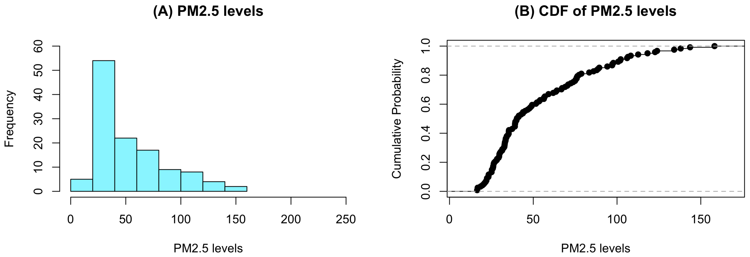
Figure 1. Histogram (A) and cumulative distribution function (CDF) (B) of daily PM2.5 levels data for Station 1.
Symmetry 18 00100 g001
Figure 2. Histogram (A) and CDF (B) of daily PM2.5 levels data for Station 2.
Symmetry 18 00100 g002
Figure 3. Histogram (A) and CDF (B) of daily PM2.5 levels data for Station 3.
Symmetry 18 00100 g003
Figure 4. Histogram (A) and CDF (B) of daily PM2.5 levels data for Station 4.
Symmetry 18 00100 g004
Figure 5. Histogram (A) and CDF (B) of daily PM2.5 levels data for Station 5.
Symmetry 18 00100 g005
Figure 6. Histogram (A) and CDF (B) of daily PM2.5 levels data for Station 6.
Symmetry 18 00100 g006
Table 1. The CPs and ALs of 95% two-sided CIs for the common percentile of BS distributions: 3 sample cases.
( n 1 , n 2 , n 3 ) ( α 1 , α 2 , α 3 ) CP (AL)
CI GCI CI BCI CI Baye CI HPD
(10, 10, 10)(0.25, 0.25, 0.25)0.93820.88740.92700.9188
(0.1926)(0.1694)(0.1849)(0.1822)
(0.25, 0.50, 0.50)0.95100.90960.94500.9410
(0.2881)(0.2396)(0.2745)(0.2691)
(0.25, 1.00, 1.00)0.94320.91660.93660.9324
(0.4762)(0.3841)(0.4483)(0.4367)
(0.50, 0.50, 0.50)0.95520.91460.94540.9470
(0.3021)(0.2462)(0.2871)(0.2827)
(0.50, 1.00, 1.00)0.94740.91520.94020.9342
(0.3843)(0.3092)(0.3632)(0.3578)
(1.00, 1.00, 1.00)0.92260.89100.92040.9160
(0.3279)(0.2576)(0.3098)(0.3066)
(10, 30, 30)(0.25, 0.25, 0.25)0.94140.91540.93860.9316
(0.1192)(0.1136)(0.1171)(0.1159)
(0.25, 0.50, 0.50)0.94200.91700.93680.9310
(0.1837)(0.1720)(0.1805)(0.1788)
(0.25, 1.00, 1.00)0.95140.93280.94660.9398
(0.2723)(0.2507)(0.2648)(0.2625)
(0.50, 0.50, 0.50)0.94940.93360.94480.9438
(0.1787)(0.1622)(0.1739)(0.1720)
(0.50, 1.00, 1.00)0.94820.93640.94680.9430
(0.2089)(0.1887)(0.2023)(0.2005)
(1.00, 1.00, 1.00)0.94160.91680.93740.9436
(0.2104)(0.1732)(0.1988)(0.1954)
(30, 30, 30)(0.25, 0.25, 0.25)0.94540.92740.93940.9370
(0.1034)(0.0998)(0.1019)(0.1009)
(0.25, 0.50, 0.50)0.94200.93140.94060.9382
(0.1491)(0.1416)(0.1470)(0.1456)
(0.25, 1.00, 1.00)0.94620.93520.94420.9408
(0.2480)(0.2259)(0.2399)(0.2367)
(0.50, 0.50, 0.50)0.95360.94340.95120.9472
(0.1514)(0.1423)(0.1489)(0.1475)
(0.50, 1.00, 1.00)0.95100.93740.94740.9486
(0.2001)(0.1807)(0.1934)(0.1914)
(1.00, 1.00, 1.00)0.94280.92500.93900.9386
(0.1669)(0.1477)(0.1611)(0.1597)
(30, 50, 50)(0.25, 0.25, 0.25)0.94660.93560.94620.9430
(0.0853)(0.0832)(0.0844)(0.0836)
(0.25, 0.50, 0.50)0.95180.94000.94980.9480
(0.1275)(0.1231)(0.1260)(0.1249)
(0.25, 1.00, 1.00)0.95120.94540.95100.9446
(0.2003)(0.1889)(0.1955)(0.1937)
(0.50, 0.50, 0.50)0.95180.94540.95020.9478
(0.1236)(0.1183)(0.1221)(0.1210)
(0.50, 1.00, 1.00)0.95300.94460.95220.9472
(0.1537)(0.1434)(0.1497)(0.1484)
(1.00, 1.00, 1.00)0.94800.93400.94000.9410
(0.1346)(0.1221)(0.1304)(0.1293)
(50, 50, 50)(0.25, 0.25, 0.25)0.94840.93760.94560.9422
(0.0791)(0.0775)(0.0783)(0.0776)
(0.25, 0.50, 0.50)0.95460.949200.95200.9492
(0.1137)(0.1102)(0.1127)(0.1116)
(0.25, 1.00, 1.00)0.95020.94100.94480.9428
(0.1867)(0.1752)(0.1818)(0.1799)
(0.50, 0.50, 0.50)0.94900.94340.94620.9440
(0.1144)(0.1102)(0.1132)(0.1122)
(0.50, 1.00, 1.00)0.95060.94260.94900.9460
(0.1499)(0.1397)(0.1458)(0.1445)
(1.00, 1.00, 1.00)0.94360.93580.94340.9418
(0.1233)(0.1133)(0.1199)(0.1189)
(50, 100, 100)(0.25, 0.25, 0.25)0.94860.94040.94420.9402
(0.0608)(0.0599)(0.0604)(0.0598)
(0.25, 0.50, 0.50)0.95160.94280.94840.9450
(0.0915)(0.0899)(0.0907)(0.0900)
(0.25, 1.00, 1.00)0.94820.94120.94640.9430
(0.1408)(0.1359)(0.1381)(0.1370)
(0.50, 0.50, 0.50)0.95380.94600.94780.9468
(0.0874)(0.0852)(0.0867)(0.0859)
(0.50, 1.00, 1.00)0.95040.94400.94840.9448
(0.1060)(0.1015)(0.1037)(0.1029)
(1.00, 1.00, 1.00)0.94540.93820.94520.9422
(0.0928)(0.0872)(0.0905)(0.0898)
(100, 100, 100)(0.25, 0.25, 0.25)0.94820.94200.94520.9426
(0.0555)(0.0548)(0.0551)(0.0546)
(0.25, 0.50, 0.50)0.94960.94560.94580.9448
(0.0797)(0.0783)(0.0791)(0.0784)
(0.25, 1.00, 1.00)0.94380.94080.94200.9390
(0.1280)(0.1232)(0.1254)(0.1242)
(0.50, 0.50, 0.50)0.95080.94180.94540.9416
(0.0795)(0.0778)(0.0789)(0.0782)
(0.50, 1.00, 1.00)0.94700.94020.94500.9436
(0.1026)(0.0980)(0.1004)(0.0995)
(1.00, 1.00, 1.00)0.94740.94460.94840.9458
(0.0837)(0.0793)(0.0818)(0.0812)
Table 2. The CPs and ALs of 95% two-sided CIs for the common percentile of BS distributions: 6 sample cases.
( n 1 , n 2 , n 3 , n 4 , n 5 , n 6 ) ( α 1 , α 2 , α 3 , α 4 , α 5 , α 6 ) CP (AL)
CI GCI CI BCI CI Baye CI HPD
(10, 10, 10, 10, 10, 10)(0.25, 0.25, 0.25, 0.25, 0.25, 0.25)0.93320.85640.91580.9084
(0.1375)(0.1246)(0.1320)(0.1305)
(0.25, 0.25, 0.25, 0.50, 0.50, 0.50)0.94780.90040.94080.9354
(0.2000)(0.1678)(0.1894)(0.1857)
(0.25, 0.25, 0.25, 1.00, 1.00, 1.00)0.94580.92060.94260.9574
(0.4280)(0.3097)(0.3867)(0.3631)
(0.50, 0.50, 0.50, 0.50, 0.50, 0.50)0.94120.90940.93760.9420
(0.2310)(0.1807)(0.2170)(0.2130)
(0.50, 0.50, 0.50, 1.00, 1.00, 1.00)0.91660.88060.91700.9336
(0.3499)(0.2558)(0.3223)(0.3120)
(1.00, 1.00, 1.00, 1.00, 1.00, 1.00)0.84700.76900.84940.8696
(0.2808)(0.1936)(0.2596)(0.2548)
(10, 10, 10, 30, 30, 30)(0.25, 0.25, 0.25, 0.25, 0.25, 0.25)0.93760.89960.92920.9236
(0.0925)(0.0885)(0.0905)(0.0896)
(0.25, 0.25, 0.25, 0.50, 0.50, 0.50)0.94660.90460.94080.9346
(0.1434)(0.1348)(0.1405)(0.1392)
(0.25, 0.25, 0.25, 1.00, 1.00, 1.00)0.95800.93580.95660.9498
(0.2346)(0.2123)(0.2270)(0.2245)
(0.50, 0.50, 0.50, 0.50, 0.50, 0.50)0.94940.93320.94440.9462
(0.1456)(0.1264)(0.1399)(0.1380)
(0.50, 0.50, 0.50, 1.00, 1.00, 1.00)0.94740.93260.94360.9428
(0.1801)(0.1571)(0.1731)(0.1714)
(1.00, 1.00, 1.00, 1.00, 1.00, 1.00)0.88020.82560.87860.9142
(0.2012)(0.1417)(0.1820)(0.1754)
(30, 30, 30, 30, 30, 30)(0.25, 0.25, 0.25, 0.25, 0.25, 0.25)0.94160.92340.93700.9316
(0.0732)(0.0713)(0.0722)(0.0716)
(0.25, 0.25, 0.25, 0.50, 0.50, 0.50)0.94360.93140.94160.9390
(0.0990)(0.0950)(0.0975)(0.0966)
(0.25, 0.25, 0.25, 1.00, 1.00, 1.00)0.94760.94160.94680.9528
(0.1759)(0.1569)(0.1687)(0.1653)
(0.50, 0.50, 0.50, 0.50, 0.50, 0.50)0.95040.94080.94700.9438
(0.1084)(0.1015)(0.1066)(0.1056)
(0.50, 0.50, 0.50, 1.00, 1.00, 1.00)0.93760.92400.93440.9442
(0.1562)(0.1373)(0.1501)(0.1479)
(1.00, 1.00, 1.00, 1.00, 1.00, 1.00)0.90420.87600.90200.9094
(0.1258)(0.1062)(0.1205)(0.1192)
(30, 30, 30, 50, 50, 50)(0.25, 0.25, 0.25, 0.25, 0.25, 0.25)0.94640.93180.94360.9416
(0.0629)(0.0616)(0.0622)(0.0617)
(0.25, 0.25, 0.25, 0.50, 0.50, 0.50)0.94680.92980.94220.9376
(0.0898)(0.0872)(0.0889)(0.0881)
(0.25, 0.25, 0.25, 1.00, 1.00, 1.00)0.95440.94700.95100.9500
(0.1509)(0.1408)(0.1465)(0.1449)
(0.50, 0.50, 0.50, 0.50, 0.50, 0.50)0.94040.93320.93820.9382
(0.0922)(0.0877)(0.0909)(0.0901)
(0.50, 0.50, 0.50, 1.00, 1.00, 1.00)0.94800.94040.94560.9448
(0.1235)(0.1133)(0.1198)(0.1187)
(1.00, 1.00, 1.00, 1.00, 1.00, 1.00)0.91000.88880.90860.9140
(0.1050)(0.0913)(0.1010)(0.1000)
(50, 50, 50, 50, 50, 50)(0.25, 0.25, 0.25, 0.25, 0.25, 0.25)0.94900.93940.94500.9394
(0.0559)(0.0550)(0.0554)(0.0549)
(0.25, 0.25, 0.25, 0.50, 0.50, 0.50)0.94560.93900.94180.9408
(0.0749)(0.0731)(0.0741)(0.0734)
(0.25, 0.25, 0.25, 1.00, 1.00, 1.00)0.94700.94040.94640.9490
(0.1262)(0.1175)(0.1224)(0.1208)
(0.50, 0.50, 0.50, 0.50, 0.50, 0.50)0.95360.94320.94960.9476
(0.0815)(0.0784)(0.0806)(0.0799)
(0.50, 0.50, 0.50, 1.00, 1.00, 1.00)0.94460.93480.94420.9460
(0.1137)(0.1045)(0.1102)(0.1090)
(1.00, 1.00, 1.00, 1.00, 1.00, 1.00)0.91580.89660.91320.9140
(0.0903)(0.0809)(0.0874)(0.0867)
(50, 50, 50, 100, 100, 100)(0.25, 0.25, 0.25, 0.25, 0.25, 0.25)0.94500.93700.94300.9406
(0.0454)(0.0449)(0.0451)(0.0447)
(0.25, 0.25, 0.25, 0.50, 0.50, 0.50)0.95060.94700.94760.9466
(0.0658)(0.0647)(0.0652)(0.0647)
(0.25, 0.25, 0.25, 1.00, 1.00, 1.00)0.95600.95080.95680.9532
(0.1066)(0.1024)(0.1044)(0.1035)
(0.50, 0.50, 0.50, 0.50, 0.50, 0.50)0.94640.94200.94560.9432
(0.0656)(0.0637)(0.0650)(0.0645)
(0.50, 0.50, 0.50, 1.00, 1.00, 1.00)0.94500.94320.94740.9450
(0.0851)(0.0808)(0.0832)(0.0825)
(1.00, 1.00, 1.00, 1.00, 1.00, 1.00)0.92820.92000.92880.9296
(0.0713)(0.0656)(0.0692)(0.0686)
(100, 100, 100, 100, 100, 100)(0.25, 0.25, 0.25, 0.25, 0.25, 0.25)0.95340.94520.95200.9492
(0.0392)(0.0388)(0.0389)(0.0386)
(0.25, 0.25, 0.25, 0.50, 0.50, 0.50)0.94660.94160.94380.9434
(0.0521)(0.0514)(0.0517)(0.0513)
(0.25, 0.25, 0.25, 1.00, 1.00, 1.00)0.94820.94280.94580.9464
(0.0845)(0.0811)(0.0827)(0.0818)
(0.50, 0.50, 0.50, 0.50, 0.50, 0.50)0.94700.94280.94360.9398
(0.0564)(0.0552)(0.0559)(0.0555)
(0.50, 0.50, 0.50, 1.00, 1.00, 1.00)0.94700.94420.94740.9484
(0.0762)(0.0725)(0.0743)(0.0737)
(1.00, 1.00, 1.00, 1.00, 1.00, 1.00)0.93380.92520.93480.9326
(0.0601)(0.0563)(0.0587)(0.0582)
Table 3. Daily PM2.5 levels data of six stations in Chiang Mai Province.
StationsPM2.5 Levels
Station 125.121.620.422.425.325.323.229.631.525.8
26.422.421.023.335.529.826.723.422.018.5
16.525.127.429.335.434.233.432.832.933.5
28.419.616.816.833.039.132.228.231.439.0
39.045.240.139.235.334.032.737.434.926.1
30.626.426.043.935.429.833.154.156.348.3
39.947.642.740.339.163.586.0101.970.356.9
66.864.151.656.4118.2143.6106.088.7112.697.2
30.133.639.341.459.153.575.967.277.375.3
97.187.9100.7108.2123.9106.5134.1158.2138.0122.7
102.246.641.243.852.261.949.349.076.497.8
89.472.459.173.869.070.994.278.776.074.9
83.4
Station 228.719.818.618.421.820.519.526.627.323.3
20.822.024.620.032.424.721.917.919.615.6
16.923.228.930.537.933.729.530.334.727.3
23.814.216.816.532.443.933.831.430.343.9
38.332.030.539.630.035.631.938.434.223.5
26.421.926.438.637.335.134.651.354.045.2
41.453.845.541.840.062.8103.9115.190.557.9
69.974.952.256.6122.6133.4106.391.1125.085.0
37.636.040.643.865.857.593.670.171.985.4
95.893.899.8111.3134.1111.0131.7157.3128.2129.8
99.341.836.539.744.860.347.647.475.386.2
95.877.956.570.361.861.877.273.871.569.3
79.4
Station 312.211.311.713.915.215.022.221.417.015.8
13.212.520.224.619.416.916.412.99.78.8
15.619.226.728.425.816.522.719.020.015.1
8.47.212.231.327.521.320.626.930.135.1
37.233.432.828.230.029.738.827.616.318.7
17.121.134.822.617.828.848.856.439.433.2
38.931.032.034.266.384.688.648.148.543.4
34.734.858.3136.6125.089.072.093.618.526.7
30.137.547.949.867.860.378.956.692.588.6
117.8106.0113.8110.9123.7155.3135.7125.585.129.3
27.635.945.051.240.247.760.878.160.842.5
58.061.559.561.858.657.867.263.3
Station 416.211.111.512.816.216.315.116.015.315.9
17.519.411.49.420.120.314.914.113.012.8
11.421.422.320.418.326.821.716.122.322.4
15.99.97.86.425.023.221.918.523.434.0
26.225.233.825.517.919.315.224.426.014.6
20.124.215.023.018.019.539.258.554.245.0
48.659.138.630.628.242.550.354.335.044.5
39.928.237.745.986.4109.774.260.750.055.3
25.731.336.548.862.144.456.253.568.969.8
82.785.1103.187.8109.7125.698.876.083.337.9
29.930.740.239.335.757.278.789.493.969.1
48.154.856.546.649.147.059.055.952.0
Station 522.212.313.711.913.515.614.717.516.313.4
17.214.712.514.623.720.615.214.318.012.6
12.313.721.121.431.228.428.520.224.322.1
17.811.19.111.631.536.421.524.128.232.3
35.336.924.729.925.928.531.429.721.723.0
28.624.927.031.136.339.637.752.649.637.8
31.543.740.035.540.288.9127.5157.0101.056.4
65.476.247.758.4137.1119.4127.9121.5161.4126.6
32.529.828.641.851.273.1117.2111.6121.0119.7
144.6155.5216.8198.5200.5175.4224.3209.9168.5151.6
155.955.250.355.255.858.549.046.274.163.7
78.166.659.4109.282.457.055.451.968.7102.7
108.6
Station 625.116.617.716.118.221.623.325.121.016.7
16.915.316.019.122.922.819.116.216.112.7
18.622.327.721.232.133.627.627.026.119.4
11.711.713.523.235.827.026.729.638.733.3
42.937.035.730.238.235.744.941.330.537.4
37.635.743.355.175.182.470.769.045.736.7
44.043.034.725.164.871.582.556.048.359.0
48.442.637.698.7147.7110.088.968.763.924.1
34.743.946.374.5119.6111.5100.5162.490.198.8
85.890.584.193.784.1132.9150.1105.575.394.6
41.230.134.540.642.838.046.171.377.461.3
52.853.154.651.749.943.647.556.553.355.1
Source: Pollution Control Department (http://air4thai.pcd.go.th/webV3/#/History, accessed on 1 November 2025).
Table 4. The estimated AIC values for the probability models using daily PM2.5 levels data from six stations in Chiang Mai Province.
DistributionsStations
Station 1Station 2Station 3Station 4Station 5Station 6
Normal distribution1185.181194.211161.231116.591306.071173.40
Log-normal distribution1131.931142.061094.121066.781208.591119.85
Weibull distribution1152.281158.751109.091077.351227.651134.86
Gamma distribution1141.221149.881102.161071.231222.821126.03
Exponential distribution1208.731206.871133.601113.571234.591178.89
Logistic distribution1183.171193.521153.431114.261298.071166.23
Cauchy distribution1201.461213.321162.791143.701286.951183.19
Birnbaum–Saunders distribution1130.671140.471093.051065.691203.671119.53
Note: Bold font means the distribution with the lowest AIC value.
Table 5. Sample statistics of daily PM2.5 levels data for six stations in Chiang Mai Province.
StatisticsStations
Station 1Station 2Station 3Station 4Station 5Station 6
n i 121121118119121120
α i 0.61260.65750.77470.69110.98330.6593
β i 56.710455.513642.708130.739162.848147.8938
θ ^ i 26.357724.462316.418313.020919.141121.0598
V a r ^ θ ^ i 3.49073.40522.07951.06934.01612.5570
Table 6. The 95% two-sided CIs for the common percentile of BS distributions, based on daily PM2.5 level data from six stations in Chiang Mai Province.
ApproachesConfidence Intervals
LowerUpperLength
GCI15.211717.53982.3281
Bootstrap15.331617.66172.3301
Bayesian15.315517.61432.2988
HPD15.263817.53982.2760
Note: Bold font indicates the approach with the shortest length.
Disclaimer/Publisher’s Note: The statements, opinions and data contained in all publications are solely those of the individual author(s) and contributor(s) and not of MDPI and/or the editor(s). MDPI and/or the editor(s) disclaim responsibility for any injury to people or property resulting from any ideas, methods, instructions or products referred to in the content.