NURBS Morphing Optimization of Drag and Lift in a Coupe-Class Vehicle Using Symmetry-Plane Comparison of Aerodynamic Performance

Abstract

This study presents a morphing Non-Uniform Rational B-Spline (NURBS) optimization method for enhancing sports car aerodynamics, with performance evaluation conducted in the vehicle’s symmetry plane. The morphing approach enables precise, smooth deformations of rear-end and spoiler geometries while preserving shape continuity, allowing controlled aerodynamic modifications suitable for comparative analysis. Flow simulations were carried out in ANSYS Fluent 2022 using the Reynolds-Averaged Navier–Stokes (RANS) equations with the standard k-ε turbulence model, selected for its stability and accuracy in predicting boundary-layer evolution, wake behavior, and flow separation in external automotive flows. Three configurations were assessed: the baseline model, a spoiler-equipped version, and two NURBS-morphed designs. The symmetry-plane evaluation ensured bilateral balance across all variants, enabling direct comparison of drag and lift performance. The results show that the proposed morphing strategy achieved notable lift reduction and favorable drag-to-lift ratios while maintaining manufacturability. The findings demonstrate that combining NURBS-based morphing with symmetry-plane aerodynamic assessment offers an efficient, reliable framework for vehicle aerodynamic optimization, bridging geometric flexibility with robust computational evaluation.

1. Introduction

For everyday passenger vehicles, aerodynamic improvements focus on reducing drag and improving fuel efficiency while maintaining safety and comfort [1]. Efficient aerodynamic design can significantly reduce fuel consumption, enhance vehicle stability, and minimize environmental impact [2,3]. Traditional methods of aerodynamic simulation often face challenges in accurately representing complex geometries and optimizing aerodynamic drag and lift performance [4]. This study addresses the need for advanced techniques in aerodynamic optimization by employing Non-Uniform Rational B-Splines (NURBS). NURBSs offer a high level of precision in geometry representation, making them ideal for optimizing the smoothness and aerodynamic efficiency of vehicle designs [5,6,7]. Previous research has explored various methods for reducing aerodynamic drag and lift, including computational fluid dynamics (CFD) simulations [8] and wind tunnel experiment [9]. However, these methods often require extensive preprocessing work and may not fully capture the intricate details of vehicle geometries. NURBSs provide a novel solution by enabling more accurate and efficient simulations [10,11]. However, design optimization has become a critical component in engineering workflows, particularly in areas where performance and precision are closely linked [11]. In this study, we introduce a practical and efficient optimization framework designed to handle multiple design iterations with minimal computational expense. By reducing the time required for analysis without compromising the quality of the results, the method supports quicker design evaluations and facilitates more agile development cycles. The distinguishing factor of the current work is its comprehensive comparative assessment across all tested design variants. Rather than relying solely on individual performance metrics, this study emphasizes relative accuracy and behavior among the alternatives, offering a broader and more informative view of the design space. This comparative layer brings clarity to the strengths and limitations of each variant, helping to identify optimal configurations more confidently. By combining a time-efficient optimization process with a structured comparative analysis, this approach not only improves accuracy in outcome assessment but also supports more informed design choices. The framework is especially valuable in applications where small differences in geometry or configuration can lead to significant performance shifts. Achieving aerodynamic efficiency often comes down to how precisely and effectively a vehicle’s shape can be adapted during the design process. In this study, we implement a NURBS-based morphing approach that allows for smooth, controlled modifications of the vehicle geometry throughout a streamlined optimization workflow [12]. The process is divided into three main stages: preprocessing, processing, and post-processing. In the preprocessing phase, the initial geometry is carefully cleaned and adjusted, with NURBS morphing techniques applied to explore improvements in balance between accuracy and computational efficiency for predicting turbulent flow behavior around the vehicle [13,14]. Finally, in the post-processing stage, results such as velocity fields, pressure contours, and streamlines are analyzed. These are compared across both the baseline and optimized models to assess performance improvements and capture subtle aerodynamic differences. Together, this workflow offers a practical and efficient path toward optimization, allowing for detailed exploration of design variants while maintaining a strong focus on accuracy and physical insight.

2. Basis of NURBS

Within the field of digital design, one often distinguishes two main modeling forms, namely surface or polygon modeling. Mesh modeling lies as the basis for the analysis procedures of today, which are based on representing the form as an assembly of polygons. This differs from NURBS-based surface modeling where one works with interpolated, smooth surfaces. Figure 1 shows some examples of the two descriptions:

2.1. NURBS Definition

Friction NURBS stands for Non-Uniform Rational B-Spline and is an extension of the B-spline concept. The widespread success of NURBS comes down to several factors, one of them being multiplicity as NURBS can analytically represent both fundamental geometries as the circle exactly, while simultaneously being able to represent free-form shapes as a car body [15]. NURBSs are based on a parametric definition that draws from B-splines and Bezier curves.

2.1.1. Components of NURBS Definitions

A geometric description relies on a certain set of parameters [16]. The NURBS description consists of the following entities:

[Knots]: The knot vector is an increasing $(\xi n-1\le \xi n\le \xi n+1)$ number of coordinates within the domain of the parameter space. This list of numbers controls the distribution of the basis functions over the domain.

[Control Points]: The control points are a list of geometric points in physical space through which the curve or surface is interpolated.

[Weights]: In NURBS, opposed to B-splines, each point is associated with a certain weight. The greater the weight for a point, the larger the effect on the geometry. Weights were introduced mainly to be able to construct exact representations of, for example, circles [17].

[Degree]: The degree means the interpolator degree of a curve. This affects the structure of the knot vector and the smoothness of the curve. The larger the degree, the more control points are active in a knot span.

2.1.2. Knot Vector

The knot vector is given as: Ξ = {ξ0, ξ1, … ξn + p + 1}. A knot vector splits the domain into a set of knot spans. These can be categorized into zero and nonzero knot spans, where the nonzero knot spans are those that are spaced along the curve. At each knot, one basis function becomes active and another becomes deactivated. A basis function Ni spans from $\xi \mathrm{i} \mathrm{t}\mathrm{o} \xi \mathrm{i}+\mathrm{p}+1$. Each knot span, therefore, has p + 1 active points. Each knot can occur multiple times, which will affect the continuity of the geometry. The first and last knots always have multiplicity p + 1. Knots can be uniformly or non-uniformly distributed. Knot vectors can be open or closed. If it is open, the last points are always fully interpolated.

2.1.3. B-Spline

The mother of the NURBS curve is the B-spline. We will start with a description of the B-spline, which will then be further extended into the full NURBS description. A B-spline curve or surface is based on the interpolation of the control points using a set of basis functions, one for each point. The basis function here refers to a similar polynomial as is found in the Galerkin discretization in classical FEA [17]. A B-spline curve is given as follows:

$$C(\xi ) = \sum N^i {\left(\xi \right)P }^i$$

(1)

where N is the basis function and P is the corresponding control point.

The table below shows the knot vectors associated with the curves shown in Figure 2. They all have the same number of points and, therefore, the same amount of basis functions. However, the amount of nonzero knot spans reduces with each degree elevation. For five points, a degree higher than four is impossible. The smoothness increases with each degree elevation. This is due to the order of the basis functions. As the degree increases, more and more points are activated at the same time. In the linear curve, each knot span is affected by two points. In the last p = 4 curve, the whole curve is one single span, meaning that all points are active over the whole curve, with varying effects. The table below shows the knot vectors for the four examples (

Table 1. Knot vectors for the curves in Figure 2.

P	Knot Vector
1	[0  0  0.25  0.5  0.75  1  1]
2	[0  0  0  0.33  0.66  1  1  1]
3	[0  0  0  0  0.5  1  1  1  1]
4	[0  0  0  0  0  1  1  1  1  1]

).

2.1.4. Basis Functions

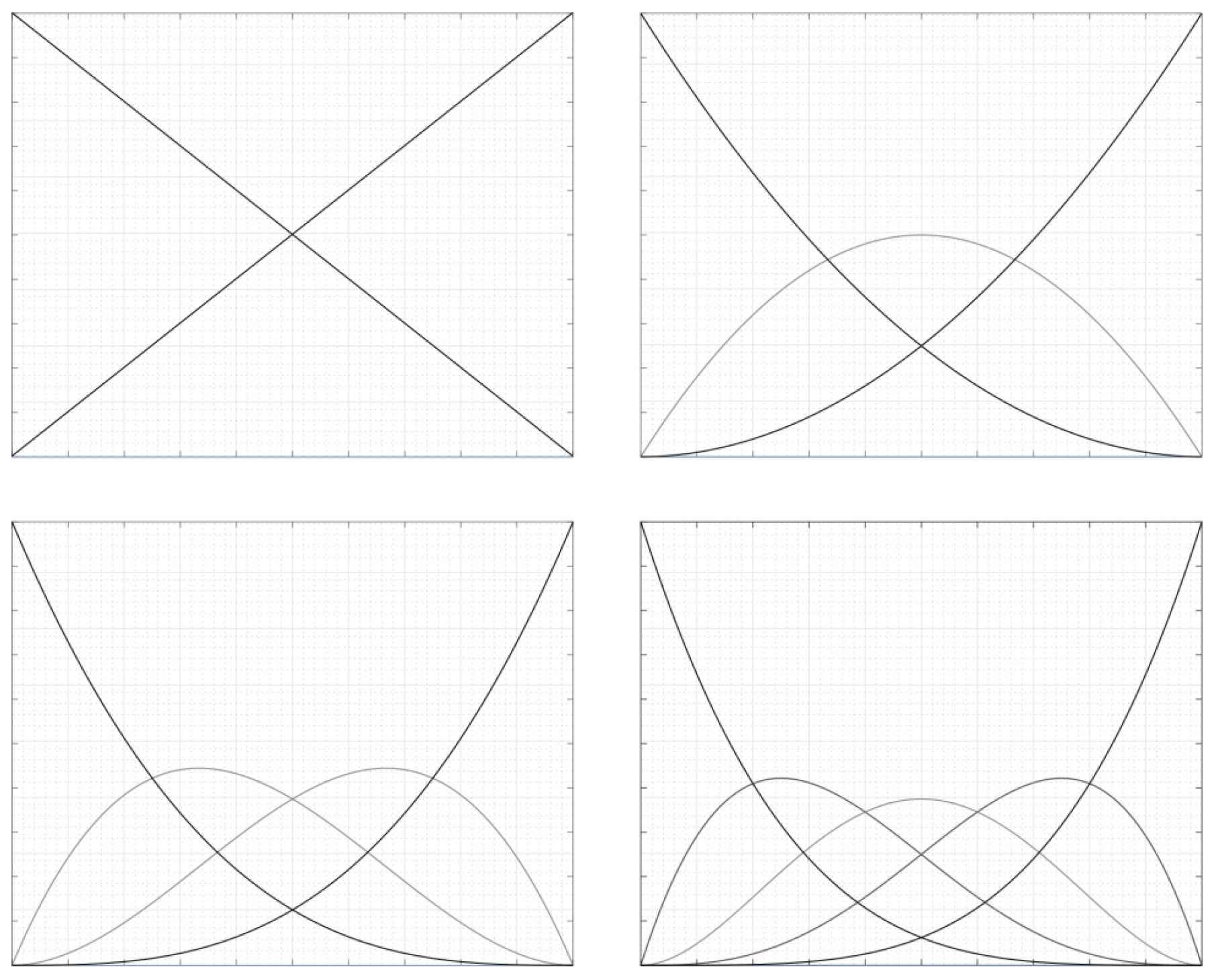
The basis functions are polynomials that give the influence of each point at a given parameter. Each control point in a curve is associated with a corresponding basis function. The distribution of basis functions along the domain is given by the knot vector and the degree [18]. An example of some single-span basis functions is given in Figure 3 below:

Given a knot vector and a polynomial degree, a Cox–deBoor recursive formula is used to compute the basis functions. In order to compute the basis functions for an interpolation of degree p, one needs the basis functions for p − 1 [20]. Therefore, the definition starts with the piecewise constant functions of the 0th degree functions. In each knot span, there are p + 1 active basis functions.

$$N_{i,0}\left(\xi \right)=\left\{\begin{array}{c} 1 if {\xi }_i\le \xi \le {\xi }_i\\ 0 otherwise\end{array} \right.$$

(2)

which states that the basis function is equal to 1 in the corresponding knot span; otherwise, it is zero. From this, the basis for p ≤ 1 interpolation can be found as

$$N_{i,p}={\displaystyle \frac{\xi -{\xi }_i}{{\xi }_{i+p}-{\xi }_i}}{N}_{i,p-1}\left(\xi \right)+{\displaystyle \frac{{\xi }_{i+p+1}-\xi }{{\xi }_{i+p+1}-{\xi }_{i+1}}}{N}_{i+1,p-1}(\xi )$$

(3)

The derivative of a parametric curve can be found as (in 2d)

$$C^{\prime }\left(\xi \right)=\left[{\displaystyle \genfrac{}{}{0pt}{}{x_{1,\xi }}{x_{2,\xi }}}\right]$$

(4)

Thus, the slope of a curve can be found through the derivative of the basis functions.

2.1.5. NURBS Basis

The NURBS basis extends the B-spline definition to a 4D space. Each point now consists of Pi [xi, yi, zi, wi], where w denotes the weights. The NURBS curve is the projection of this onto 3D space, meaning it can be dealt with similarly to the previously mentioned B-splines [21]. The definition of the NURBS basis functions is given by:

$$R_i^p={\displaystyle \frac{N_{i,p}\left(\xi \right)w_i}{{\sum }_{j=1}^n{N}_{j,p}\left(\xi \right)w_j}}$$

(5)

Giving the function for a NURBS curve as:

$$C\left(\xi \right) = R_i^p\left(\xi \right)P_i$$

(6)

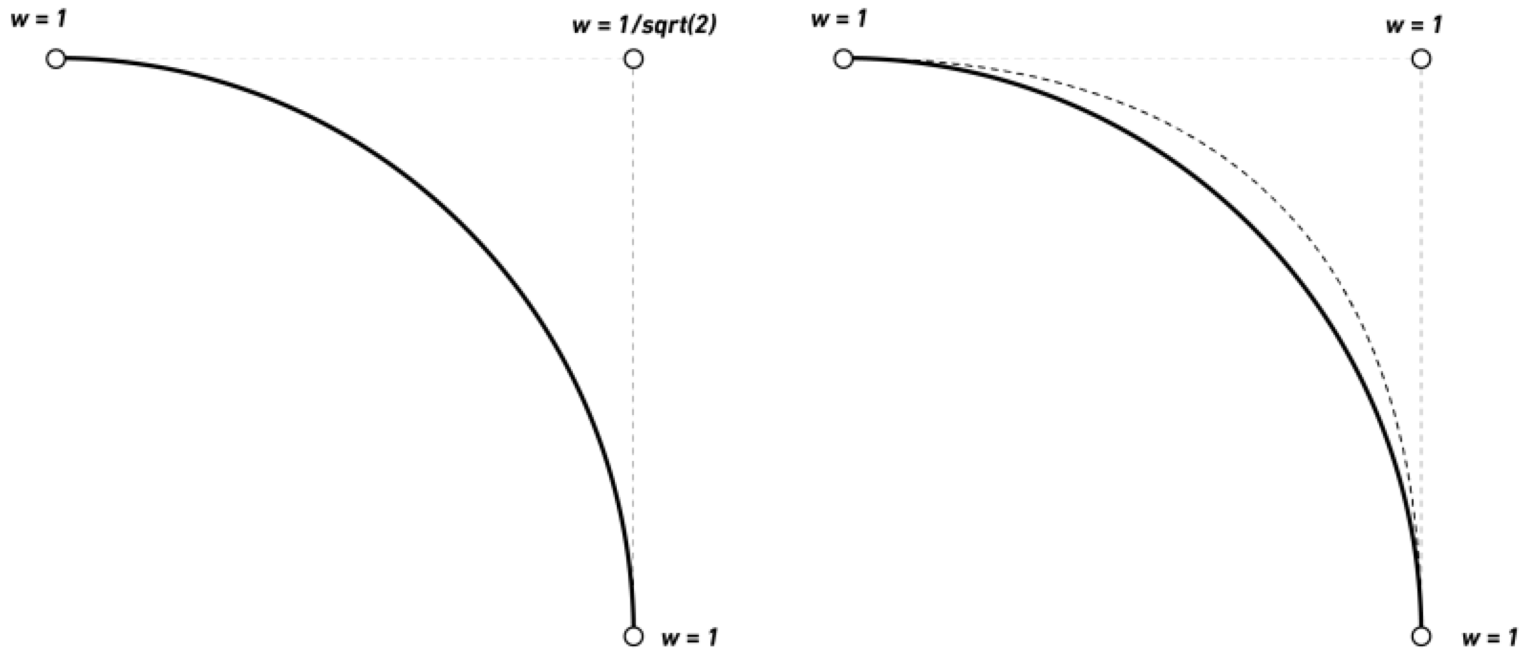
The main motivation for extending B-splines into NURBS is the possibility to represent exact analytical geometries such as circles when weight alters the influence of specific points. Figure 4 shows a second-degree curve, one where the weights are modified to match a perfect circle. The simple second-order polynomial will not have a constant curvature and will, therefore, deviate from the perfect circle.

2.2. NURBS Surfaces

The definition for a surface, which is the relevant geometry for this thesis, has the same logic as the curve but extended to a grid. Each point is then associated with two basis functions, one in each direction [22]. The definition is as follows.

$$S\left({\xi }_1,{\xi }_2\right)=\sum _{i=1}^n\sum _{j=1}^n{N}_{i,p}\left({\xi }_1\right)M_{j,q}\left({\xi }_2\right)P_{i,j}$$

(7)

In the context of B-spline surfaces, we can think of S as the surface itself. The basis functions that help shape this surface are represented by n and M, which operate in two different directions. The indices i and j identify specific basis functions, while p and q represent the degrees of interpolation for those directions. Lastly, P is a point located within the network of control points that define the overall shape of the surface.

The underlying base for any NURBS surface is always a two-dimensional grid of points. However, the number of points can vary in each direction, and they can have independent interpolation degrees. A NURBS model is mainly composed of several surfaces, which will be referred to as patches. Within a patch, the continuity is given as p − 1, but as the end points are interpolated, the continuity of basis functions will not follow over patch intersections.

2.3. Differential Geometry

When dealing with NURBS as a geometry basis, one deals with the representation of parameterized smooth objects. The field of differential geometry is concerned with the study of curved objects in space. It will, therefore, provide some concepts and tools needed to be able to compute the necessary quantities, regarding stresses and strains in smooth continuous bodies. However, this section builds upon what is presented by C. Williams [15].

As a first step, a general parameterization of a curved body in three-dimensional space is needed. The body of a surface can be parameterized as:

$$X(\theta 1, \theta 2) = x(\theta 1, \theta 2)e1 + y(\theta 1, \theta 2)e2 + z(\theta 1, \theta 2)e3$$

(8)

In Equation (8), X represents a point on the body of the surface, while the terms x, y, and z are functions of the surface parameters θ1 and θ2. The expression is constructed using the Euclidean base vectors e1, e2, and e3, which correspond to the three dimensions of space. The parameters θ1 and θ2 are used to define the position on the surface.

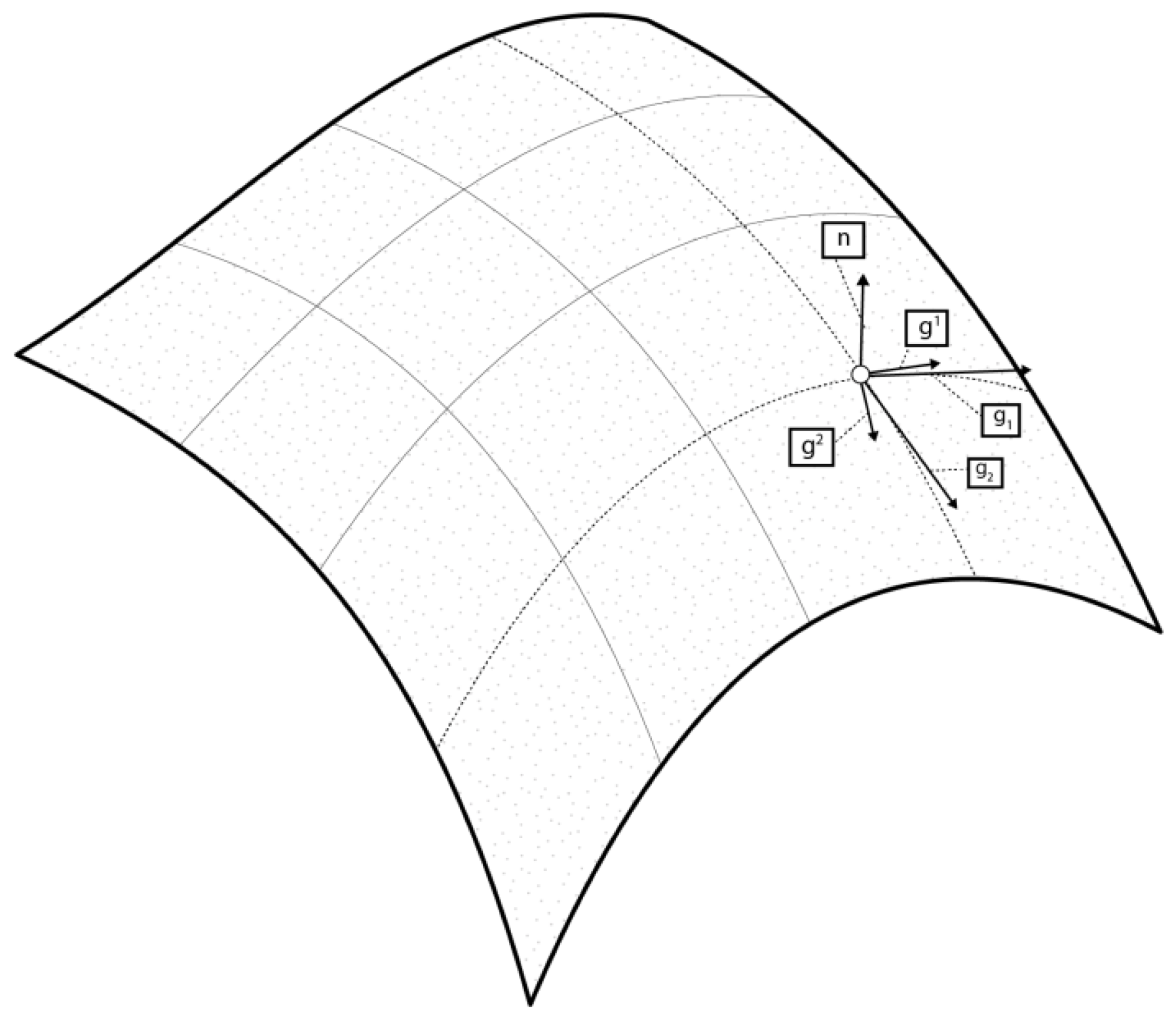
When dealing with quantities related to a curvilinear coordinate system, a set of vectors is necessary to treat these quantities. The theories presented will refer to two sets of vectors needed to deal with this type of geometry. In Figure 5, a set of vectors is drawn. These show the covariant base vectors [g1, g2] along with the contravariant base vectors [g1, g2] and the normal vector [n]. The covariant base vectors are given by the differentiation of the parameterization with respect to the parameter variable

$$g_i={\displaystyle \frac{ \partial X }{\partial {\theta }_i}}$$

(9)

with the normal vector n given by:

$$n={\displaystyle \frac{ g_1\times g_2}{\left|g_1\times g_2\right|}}$$

(10)

The covariant base vectors can be used to define a local cartesian basis at an arbitrary point on the shell body. This is given as: (the hat refers to a local coordinate system)

$${ê}_1={\displaystyle \frac{ g_1 }{\left|g_1\right|}} \& {ê}_3=n$$

(11)

$${ê}_2={\displaystyle \frac{ g_2-(g_1.g_2)g_1 }{‖g_2-(g_1.g_2)g_1 ‖}}$$

(12)

However, as the base vectors g_i are curvilinear and, therefore, are not necessarily perpendicular, another set of base vectors is useful, namely, the contravariant base vectors g_i. The essential property of the contravariant vectors is that they are perpendicular to their respective contravariant vector. Further, they also lie on the tangent plane of g_i and are perpendicular to n. They, therefore, possess the following relationship:

$$g_i · g^j = {\delta }_{ij}$$

(13)

$$g_i·n=g^j.n=0$$

(14)

The magnitude of the contravariant vectors is coupled to that of the covariant vectors through $g_i·g^j={\delta }_{ij}$. The reason for the need of these vectors lies in the fact that computing dot products between curvilinear base vectors creates spurious off-diagonal terms, which is circumvented by using a combination of co- and contravariant bases.

3. Problem Setup

3.1. Turbulence Modeling

The simulations in this study were performed using ANSYS Fluent, which incorporates the Reynolds-Averaged Navier–Stokes (RANS) framework with a range of turbulence models. The numerical setup follows the immersed boundary projection method (IB), as described in [20], adapted within the solver to handle the complex vehicle geometry and flow interaction.

The velocity and pressure fields are decomposed using the Reynolds-Averaged Navier–Stokes (RANS) approach [23], which requires a closure model to represent the influence of turbulent fluctuations on the mean flow. In this work, the standard k-ε formulation is adopted. This approach solves two additional transport equations, one for the turbulent kinetic energy (k) and another for its dissipation rate (ε), allowing the RANS system to account for turbulence effects without incurring the high computational demands of more complex models.

For external flows around road vehicles, the k-ε model offers a dependable compromise between accuracy and efficiency. It captures the essential characteristics of boundary-layer development, wake formation, and flow separation, all of which are critical to estimating aerodynamic forces such as drag and lift. Its proven stability under a wide range of flow conditions also makes it particularly suitable for iterative optimization, including the NURBS-based geometry modifications explored in this study. The formulation used follows the framework introduced by Launder and Spalding [24], which remains a reference point in engineering applications.

The suitability of this turbulence treatment is reinforced by the configuration detailed in Section 3.2, where the computational domain and boundary conditions are tailored to complement the near-wall modeling strategy of the k-ε approach, ensuring accurate resolution of both the boundary layer and the wake region.

3.2. Domain and Boundary Conditions

3.2.1. 3D Model

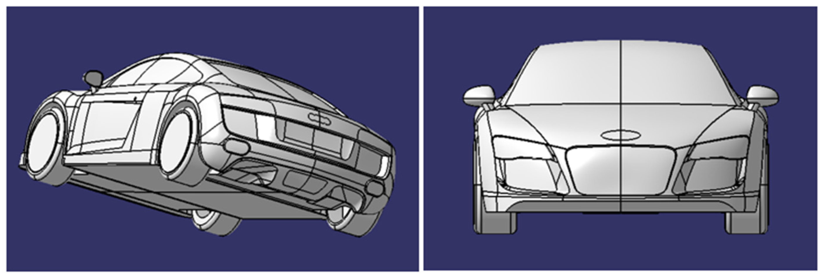
In this research, the Audi R8 (with mirrors and smooth underbody) is selected as the car model. The three-dimensional geometrical modeling values of the AUDI R8 are given in

Table 2. Audi R8 dimensions [25].

Specification	Details (mm)
Length	4426
Width	2037
Height	1240
Ground clearance	110
Wheel base	2650
Front tread	1599
Rear shoulder room	1454

. Further, the other dimensions were obtained using the 3D tracing of the car profile using commercial CAD Software 2021, as shown in Figure 6.

3.2.2. Boundary Conditions

The chosen wall function for the viscosity term applies a continuous turbulent viscosity profile near the wall, based on the local velocity, following the approach proposed by [26]. The divergence terms are calculated using the default Gauss linear scheme. For the velocity convection term, the bounded Gauss linearUpwindV scheme is applied to the velocity gradient. This approach helps maintain stability when dealing with convection terms, particularly in areas with steep velocity gradients [27], ensuring second-order accuracy. Gradient calculations use the Gauss linear method, with a multi-dimensional limiter applied to improve solution stability as well. The quantities of interest include the 3D velocity field, surface pressure, wall shear stresses, and aerodynamic coefficients.

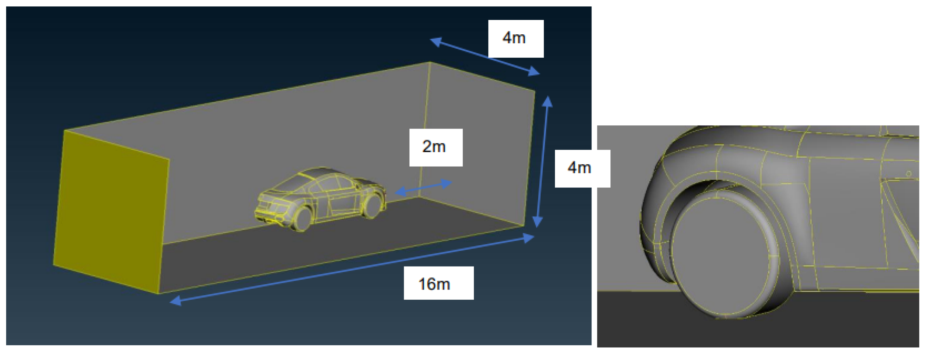
To prevent backflow into the simulation domain (Figure 7), the outlet velocity boundary condition was set as an inlet–outlet condition. The car surface and ground were assigned no-slip conditions, while the wheels were modelled with the rotating-Wall-Velocity boundary condition. Slip conditions were applied to the lateral and top boundaries of the domain. To account for near-wall viscosity effects, the nut-U-Spalding-Wall-Function approach was used [28].

A 1:1-scaled 3D fastback car body model was chosen for the CFD simulations. The simulations were performed using commercial software. In this study, pressure and velocity coupling is handled by the SIMPLE algorithm (Semi-Implicit Method for Pressure-Linked Equations), as implemented in the CFD 5-2024 solver, which is specifically designed for steady-state, turbulent, and incompressible flow simulations. The k-epsilon model, based on [24], was chosen for the Reynolds-Averaged Navier–Stokes (RANS) simulations due to its ability to overcome the limitations of the standard turbulence model, particularly its effectiveness in predicting flow separations that have a significant impact on the drag and lift coefficients.

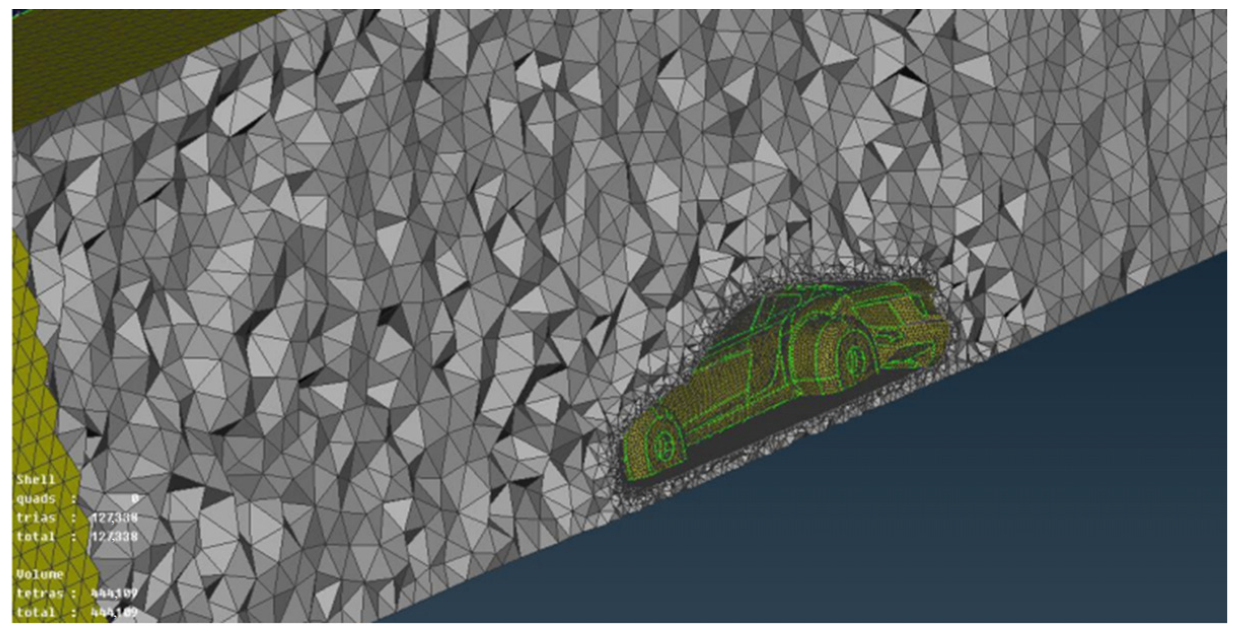
The simulations were conducted at a flow velocity (U∞) of 30 m/s, which corresponds to a Reynolds number of approximately 9.39 × 10⁶, using the car length as the characteristic length scale. The computational mesh is performed using the Snappy-Hex-Mesh (SHM) tool [29]. The mesh includes four distinct refinement zones, as illustrated in Figure 8. Additional layers were added around the car body to accurately capture the wake dynamics and the evolution of the boundary layer. Boundary conditions were specified with a uniform velocity at the inlet and pressure-based conditions at the outlet.

4. Results and Discussion

The lift coefficient CL and drag coefficient CD are essential dimensionless parameters that describe the aerodynamic performance of a body moving through a fluid [30]. The lift coefficient quantifies the lift force, which acts upward against the oncoming airflow. This force is primarily influenced by the distribution of pressure over the object’s surface. In contrast, the drag coefficient measures the drag force, which acts in the direction of the airflow. Drag is caused by pressure differences (pressure drag) and viscosity effects (skin friction drag). Both coefficients are affected by several factors, including the object’s shape and orientation, its surface properties, and the characteristics of the surrounding airflow over the car body. By relating these aerodynamic forces to fluid density, airflow velocity, and reference area, the drag and lift coefficients (described in Equation (15)) provide valuable insights into the efficiency and effectiveness of aerodynamic designs.

$$\left\{\begin{array}{c}{C}_d={\displaystyle \frac{F_d}{\frac{1}{2}\rho u_{\infty }^2{A}_{refp}}}\\ C_L={\displaystyle \frac{F_L}{\frac{1}{2}\rho u_{\infty }^2{A}_{reff}}}\end{array}\right.$$

(15)

The drag force, denoted as F_d, experienced by a body depends on effective frontal area Areff, the freestream velocity u∞, and the air density ρ. This force is made up of both pressure and frictional components.

The lift force, represented as FL, depends on its planform surface area Arefp, the freestream velocity u∞, and the air density ρ. This force is mainly generated by the pressure distribution over the body’s surface, resulting in a net force perpendicular to the freestream flow direction. In evaluating the lift coefficient, we not only analyze the aerodynamic forces but also ensure adequate mesh resolution, appropriate turbulence modeling, and sufficient computational resources to accurately capture flow characteristics, including boundary layers, separation, and wake effects.

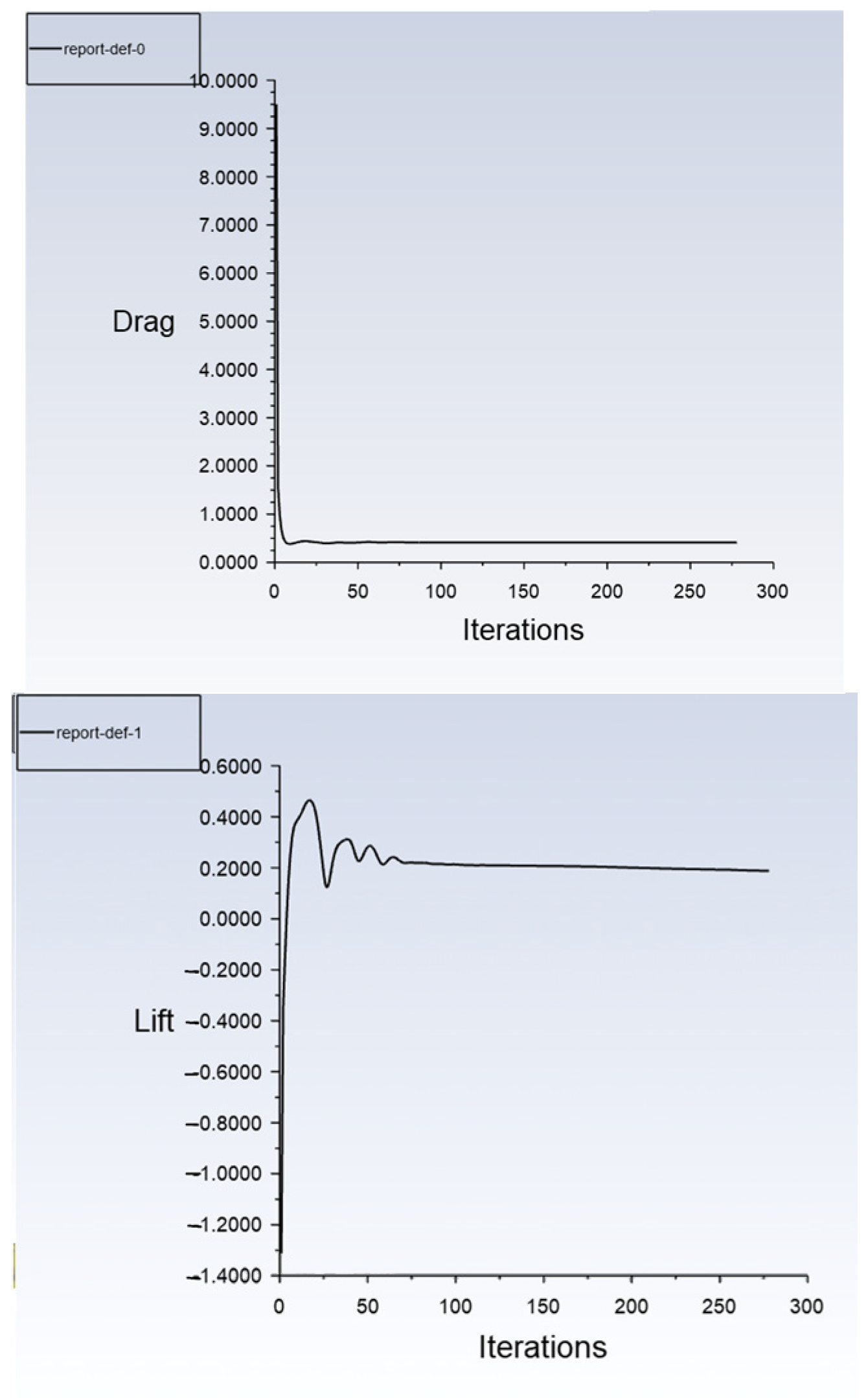
These two parameters are fixed to evaluate the convergence of the CFD simulation, as shown in the figures below.

Figure 9 illustrates the convergence histories of the drag and lift coefficients during the simulation. The drag coefficient converges to a stable value of Cd = 0.443415 after approximately 30 iterations, while the lift coefficient stabilizes at Cl = 0.184169 following initial oscillations, around iteration 100. The absence of significant fluctuations in both curves confirms that the solution has reached a steady state. These final values demonstrate good convergence behavior, indicating the numerical stability and reliability of the aerodynamic simulation.

4.1. Post-Processing of the Original Geometry

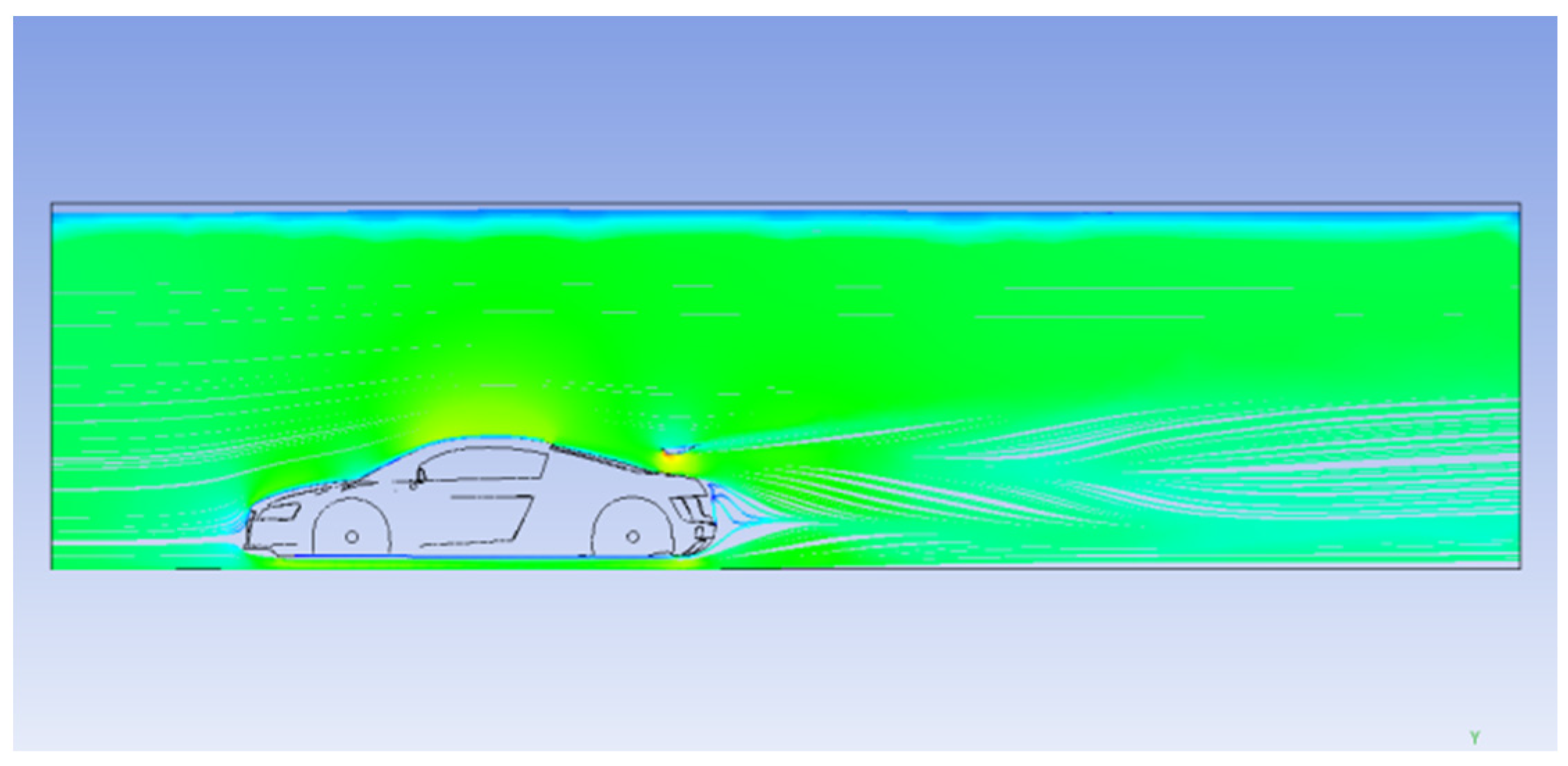
The streamlines, created using the ANSYS post-processing tool on the 2D mid-surface (symmetry plane) of the domain, are an important part of CFD analysis. They help identify areas with concentrated turbulence, which could be improved by adding aerodynamic features like a spoiler, or tweaking the car’s rear geometry to smooth out the flow. This would ultimately enhance the vehicle’s overall aerodynamic performance (Figure 10).

4.2. Geometry Optimization by Adding Spoiler to the CAD Geometry

4.2.1. Spoiler Design

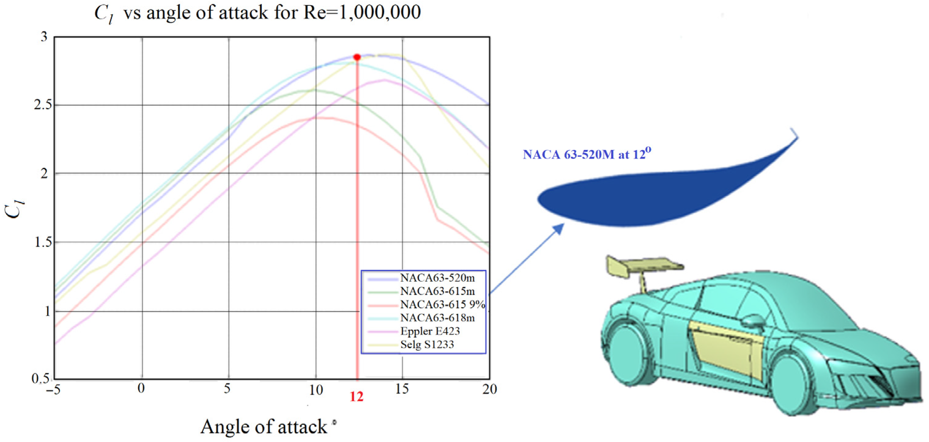
Designing a spoiler to improve a vehicle’s aerodynamic performance involves optimizing its shape, position, and integration with the overall vehicle design to achieve specific goals, such as reducing drag, increasing downforce, and enhancing stability [31]. The spoiler should be placed at the rear of the vehicle, with its height and angle precisely tuned to achieve a balance between drag reduction and downforce. A cross-section shape (see Figure 11) is chosen using open access airfoil databases [32] for optimal aerodynamic profiles, and vertical endplates minimize flow separation and turbulence, while adjustable features allow for adaptation to different driving conditions. Lightweight materials, such as carbon fiber or aluminum, are essential to avoid adding excessive weight. CFD analysis and wind tunnel testing are critical for validating performance and optimizing design. Additionally, the spoiler should align aesthetically with the vehicle, comply with safety regulations, and avoid disrupting airflow around other aerodynamic elements. Tailoring the design to specific vehicle types, such as sports cars, sedans, or SUVs, ensures maximum effectiveness in achieving aerodynamic efficiency and stability.

The Airfoil NACA63-520M is an excellent choice for an angle of attack of 12° based on the graph provided in Figure 11.

At this angle, it shows one of the highest lift coefficients CL among the compared airfoils. This characteristic makes it ideal for applications requiring significant lift performance, such as a spoiler design, where maximizing downforce is critical for stability and handling. Its superior lift properties at higher angles ensure better aerodynamic performance under these conditions.

4.2.2. Post-Processing of the Geometry with Spoiler

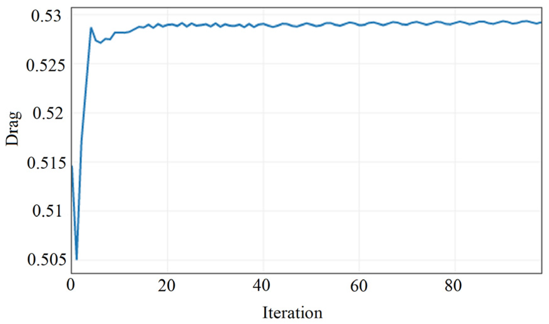
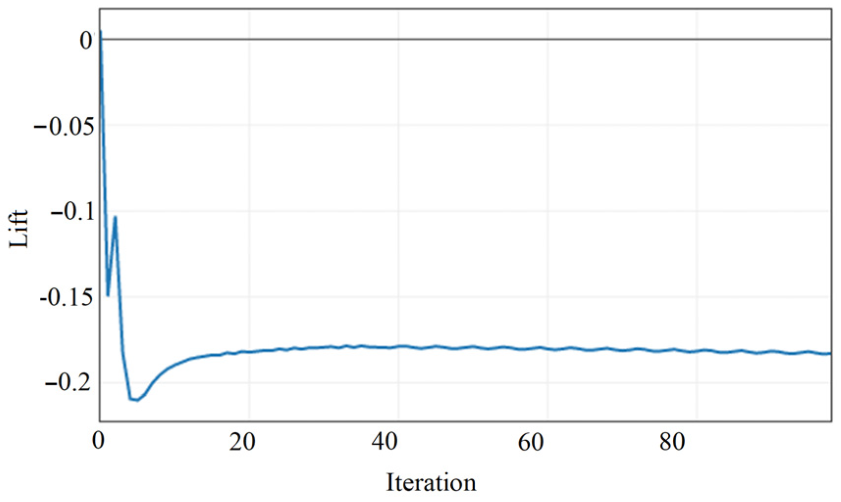
Figure 12 and Figure 13 illustrate the convergence histories of the drag and lift coefficients during the simulation of the spoiler car variant. The drag coefficient converges to a stable value of Cd = 0.529347 after approximately 40 iterations, while the lift coefficient stabilizes at Cl= −0.182030 following initial oscillations, around iteration 20. The presence of small fluctuations in both curves is due to the small changes in the pressure values over the airfoil (see figures below).

These final values demonstrate acceptable convergence, indicating the numerical stability and reliability of the aerodynamic simulation and the optimal solution (Figure 14 and Figure 15)

The reduction in the lift coefficient (Cl) compared to the original version of the vehicle (nearly −198%) is likely due to the presence of the spoiler. The primary function of a spoiler is to decrease the lift by disrupting the airflow in a controlled manner, preventing the air from separating too early and reducing the pressure difference between the top and bottom of the vehicle.

By modifying the airflow, the spoiler reduces the upward force on the vehicle, which results in a lower lift coefficient (negative Cl). This can improve vehicle stability, especially at higher speeds, as it helps maintain better contact with the road. Therefore, the reduced lift in the spoiler-equipped vehicle is an expected outcome and indicates that the spoiler is performing its intended function.

Furthermore, the increase in the drag coefficient (Cd) in the spoiler-equipped version (+19.37%) can be attributed to the disruption of airflow caused by the additional aerodynamic features, as shown by the streamlines plot. While spoilers effectively reduce lift and improve stability, they can also raise drag by promoting flow separation, turbulence, and disturbing the smooth airflow over the vehicle’s surface.

In particular, spoilers generate localized pressure differences, leading to higher resistance and, consequently, an increased drag coefficient. The changes in the boundary layer and vortex formation around the spoiler further contribute to the drag increase.

Although the spoiler reduces lift, it may not necessarily reduce drag or could even increase it, depending on factors such as its design, size, and positioning. The increase in Cd is likely a trade-off for enhanced vehicle stability and overall aerodynamic performance.

However, this rise in drag presents an opportunity for innovative optimization. Using advanced techniques like NURBS to modify the entire rear structure of the vehicle could help refine the aerodynamic design, potentially reducing drag while maintaining or improving lift reduction and stability.

4.3. Design Parameter Optimization Using NURBS

Several geometric parameters with significant impact on aerodynamics were selected and varied within a specific range. These parameter ranges were chosen to avoid values that are either difficult to manufacture or not aesthetically pleasing [33].

For our cases, we will focus on the impact of the Trunklid using the NURBS Morph Box moving technique (Figure 16).

NURBS Morphing Optimization

For the methodology, detailed in Section 2, the procedure involves deforming sets of NURBS surfaces by adjusting the Box morphing control points symmetrically while preserving geometric continuity. This results in the original CAD models being modified, which are then exported as meshed surfaces. The workflow also includes adapting the CFD surface grid of the reference shape to the deformed MorphA and MorphB variants. To do this, the NURBS parametric coordinates of each surface grid node must be determined.

After the morphing process, the displacement of the trimming curves in the NURBS parametric space guides the Radial Basis Function (RBF)-based displacement of the nodal parametric coordinates’ points [34].

As shown below, two alternative designs have been proposed as potential improvements to the original car body.

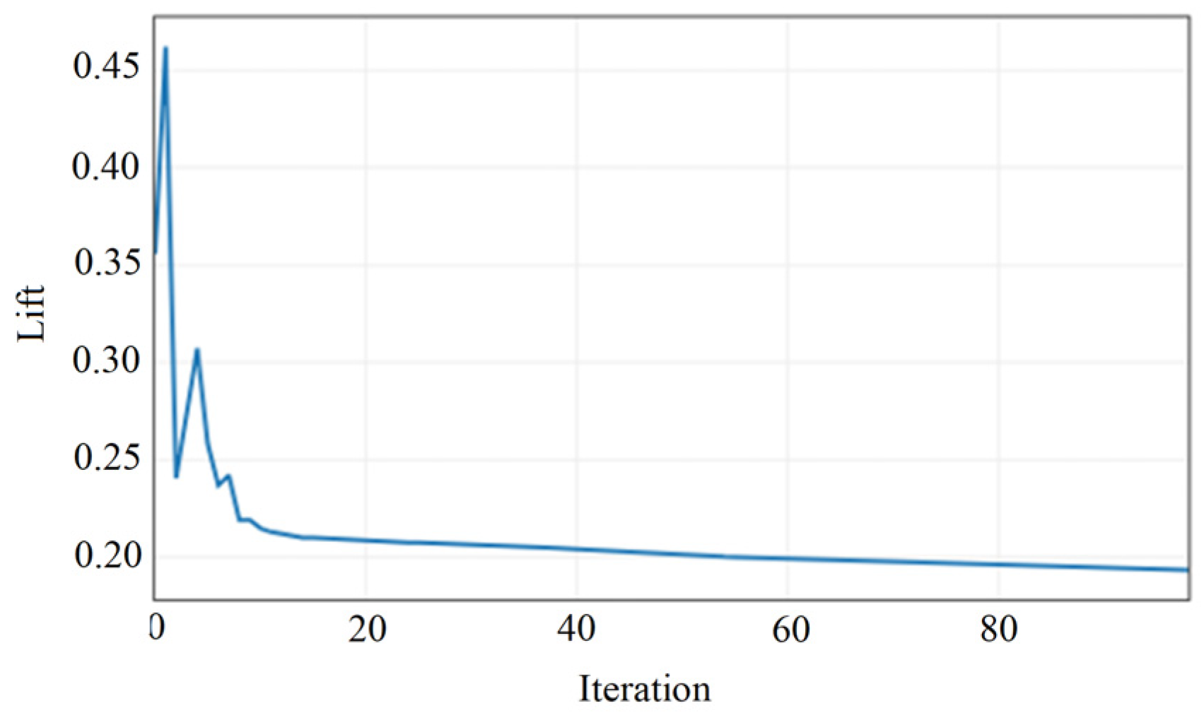
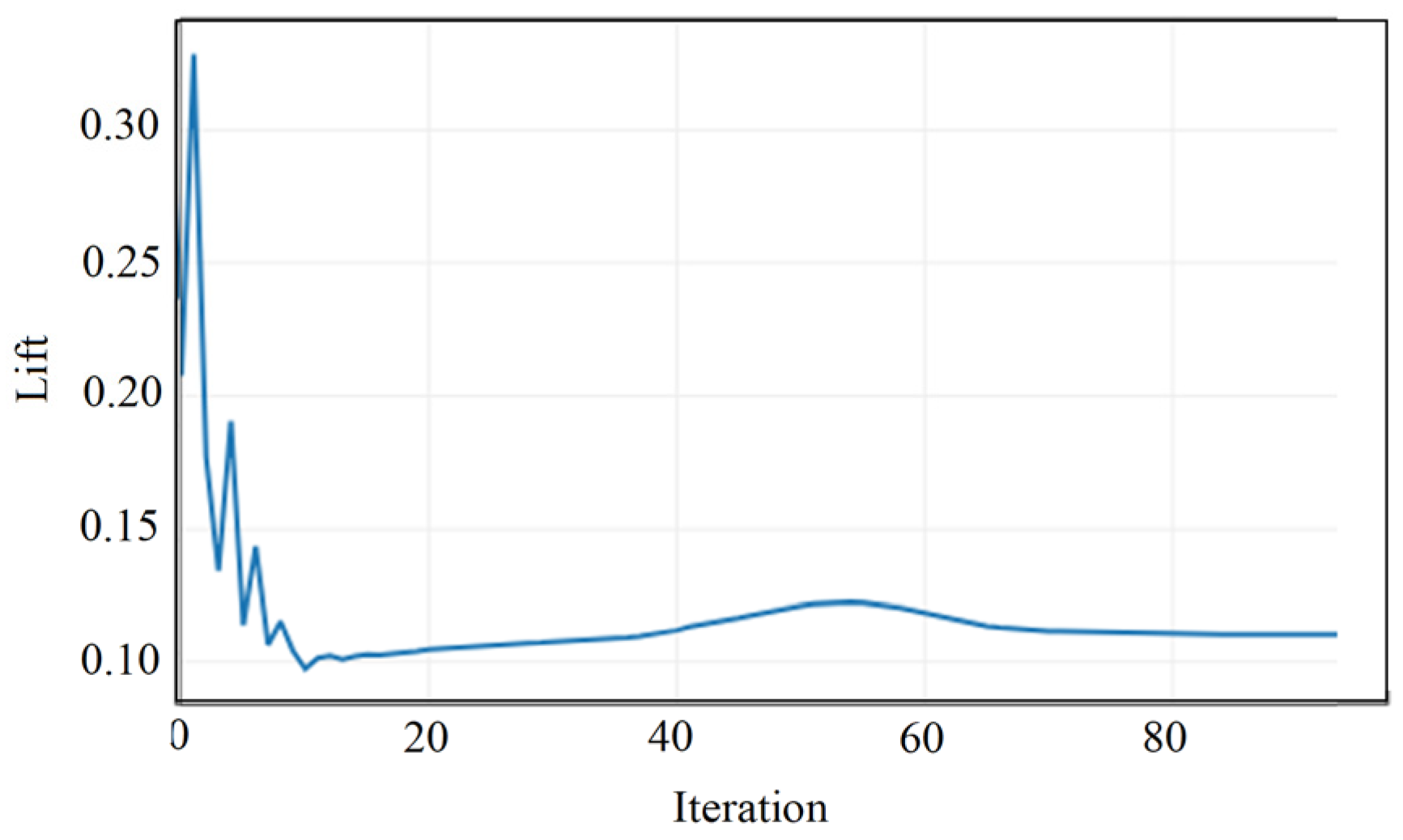
The first, Variant Morph A shown in Figure 17, involves slightly tilting the front surface to minimize air stagnation in that region. This adjustment helps to smooth the airflow and reduce drag. Additionally, the rear length of the vehicle has been extended to enhance wake management, reducing turbulence and improving overall aerodynamic efficiency. The Morph B variant (Figure 18) has a mini spoiler added to the rear shape of the car to obtain negative lift. The height of the model has been slightly reduced, and the angle of attack of the air flowing over the upper part of the model has been slightly increased (Figure 19, Figure 20, Figure 21 and Figure 22). These adjustments were made using commercial preprocessing software, which include morphing box CAD modification functions.

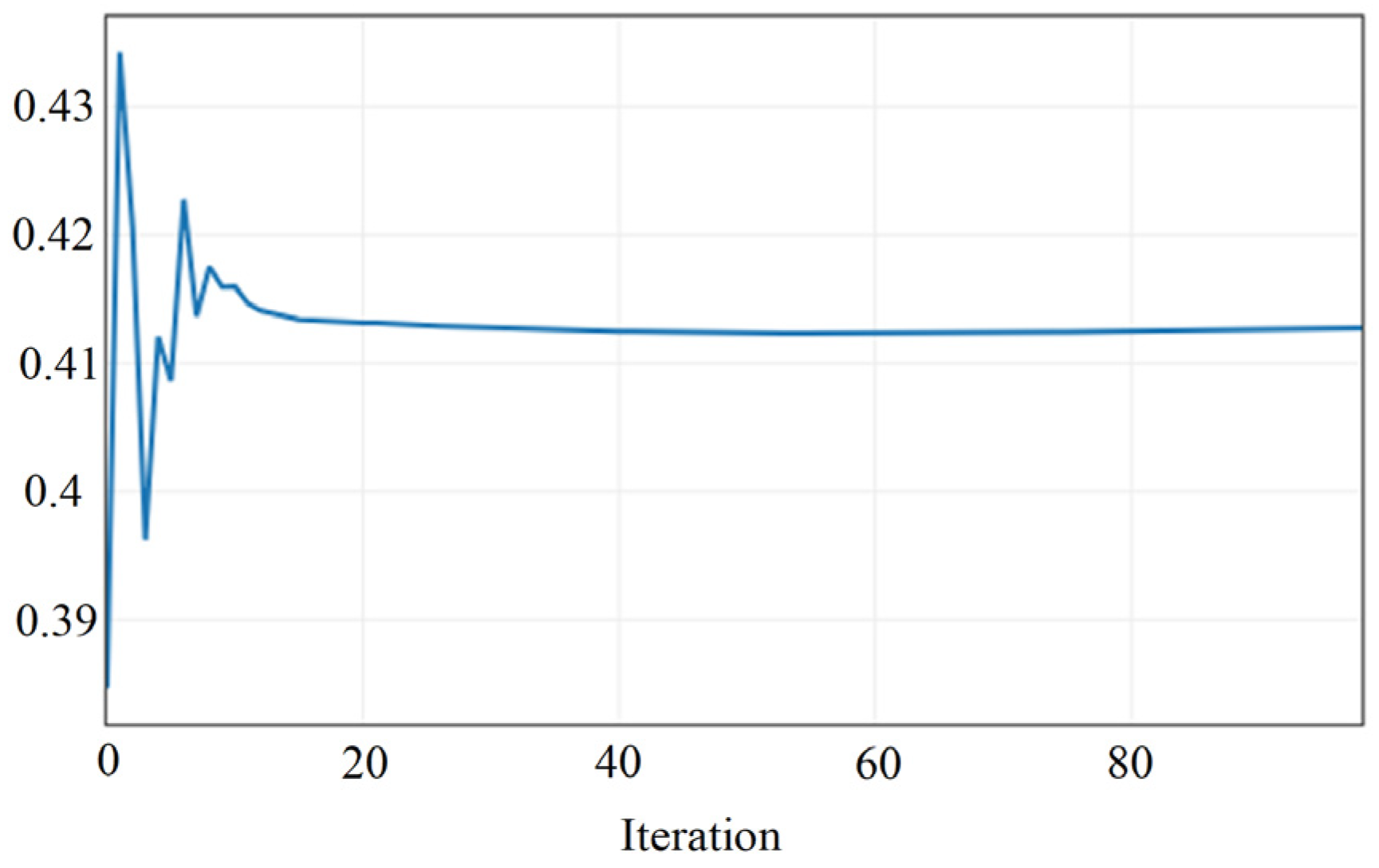
For Morph A, the convergence histories of the drag and lift coefficients show that the drag coefficient (Cd) stabilizes at 0.412729, while the lift coefficient (Cl) settles at 0.193074.

For Morph B, the drag coefficient (Cd) is slightly higher at 0.445455, and the lift coefficient (Cl) reduces to 0.110303. This shows that while Morph B leads to a more significant reduction in lift, it comes at the cost of a slight increase in drag.

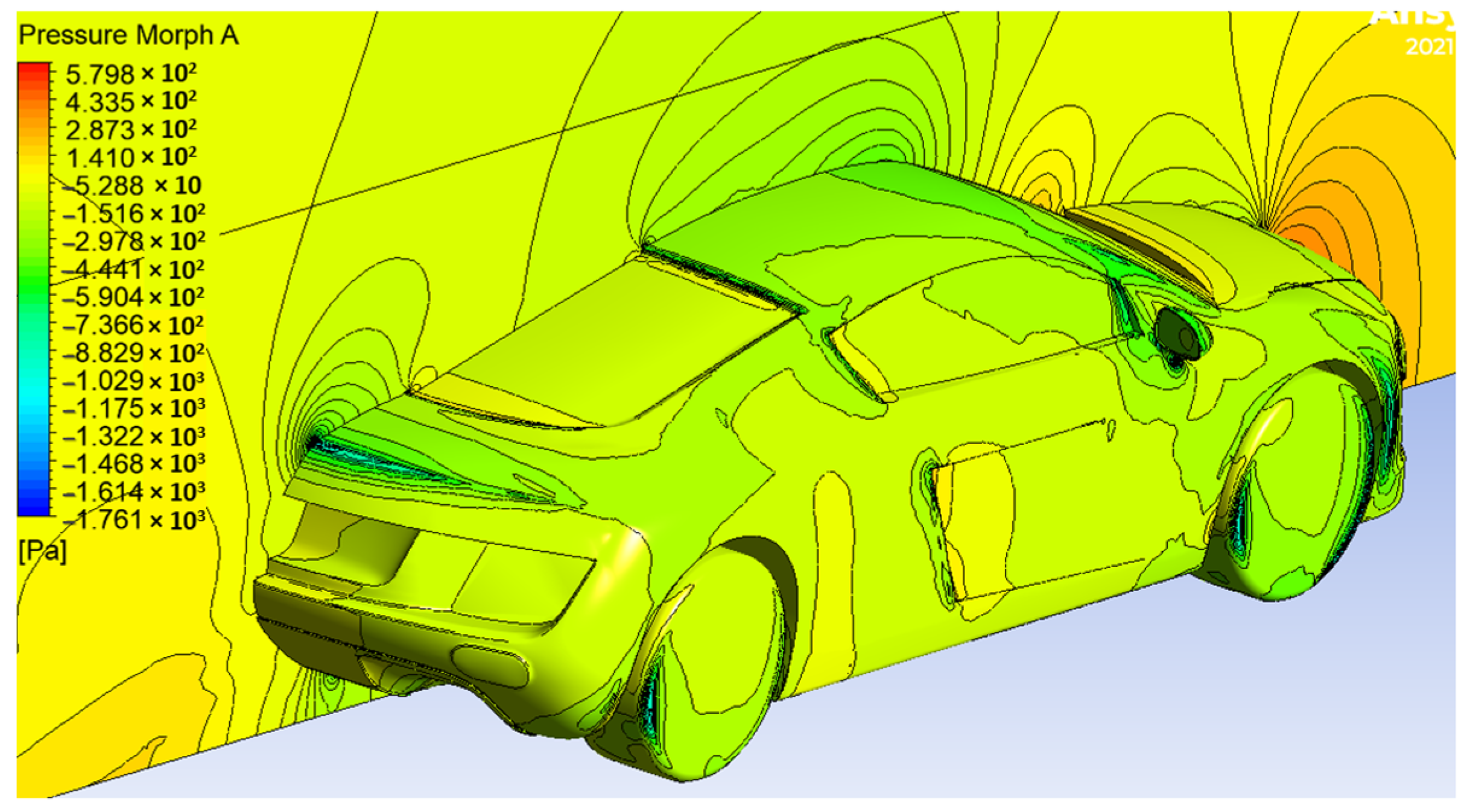
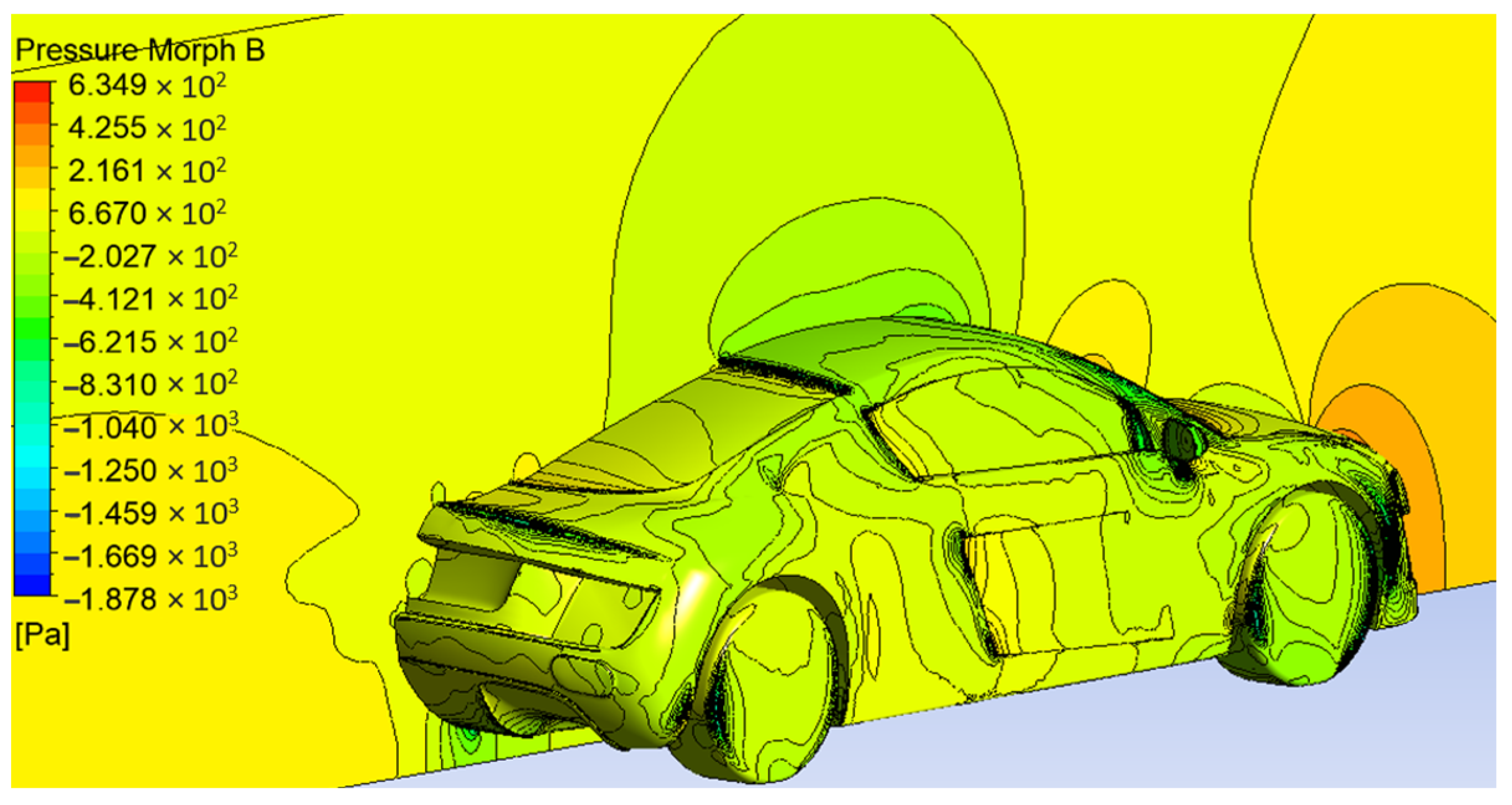
Figure 23 and Figure 24 show the surface pressure distribution over the vehicle body for both Morph A and Morph B, focusing on the rear area to highlight the differences between the two designs.

For Morph A, the pressure distribution at the rear shows a greater concentration of low-pressure regions around the rear end, side mirrors, and the underbody region. Consequently, this can lead to higher lift and reduced stability at high speeds.

In contrast, Morph B exhibits a more optimized pressure distribution at the rear, achieved through the addition of a mini spoiler and modifications to the rear geometry created by the NURBS Box morphing modification, as shown in Figure 17 and Figure 18. The low-pressure region is better controlled, with a smoother wake transition. This design significantly reduces lift and improves the flow around the rear of the vehicle, enhancing aerodynamic stability. While a low-pressure zone remains around the rear and underbody, the wake is more compact and organized, indicating aerodynamic improvements that minimize drag and optimize overall vehicle performance. The differences in rear pressure distribution between Morph A and Morph B clearly demonstrate how the aerodynamic changes in Morph B, especially at the rear, lead to better wake management and a more stable airflow, ultimately reducing lift and potentially lowering drag.

4.4. Comparative Analysis Framework

In this section, a comparative analysis framework is implemented to select the optimal variant of the car that meets the desired aerodynamic performance. To achieve this, three vertical axes are defined on the mid-surface (symmetry plane) of the domain at different distances from the origin of the absolute coordinate system: Z = 6 m, Z = 10 m, and Z = 11 m (Figure 25). These control axes are positioned at the rear of the car to more effectively evaluate several key aerodynamic parameters.

4.4.1. Pressure Coefficient

The pressure coefficient (Cp) is a dimensionless parameter used in aerodynamics to describe how pressure varies over a surface in relation to the freestream pressure. It offers a method for comparing the pressure distribution on a body’s surface, such as a vehicle, relative to the dynamic pressure of the fluid flow [35]. The pressure coefficient is calculated using the following formula:

$$U=\sqrt{U_x^2+U_y^2+U_z^2}$$

(16)

4.4.2. Velocity Magnitude

Velocity magnitude refers to the speed of the air at a given point. It is a scalar quantity that represents how fast the fluid particles are moving at that location. The velocity magnitude is used to describe the speed of the airflow over the vehicle and is essential for calculating other parameters like dynamic pressure and the Reynolds number [36].

The velocity magnitude (U) at any point in a flow field is calculated as:

$$U=\sqrt{U_x^2+U_y^2+U_z^2}$$

(17)

where: U_x, U_y, U_z are the velocity components in the x, y, and z directions, respectively.

In aerodynamic studies, the velocity magnitude is used to determine the dynamic pressure $\left({\displaystyle \frac{1}{2}}{\rho U}^2\right)$ and to evaluate the flow characteristics around the vehicle’s surface, including the formation of turbulence, acceleration, or deceleration of the air. This information is essential for evaluating the aerodynamic forces acting on the vehicle, including drag and lift.

4.4.3. Turbulent Viscosity

Turbulent viscosity, or eddy viscosity, is a concept used in fluid dynamics to model the effects of turbulence on the airflow around the vehicle. In turbulent flows, the chaotic motion of fluid particles causes fluctuations in velocity and mixing between fluid layers [37]. Turbulent viscosity quantifies the enhanced momentum transfer due to these turbulent eddies, which plays a significant role in determining aerodynamic performance, including drag and lift.

Turbulent viscosity is used in turbulence models to simplify the complex behavior of turbulent flows. In the most common models, such as the k-ϵ model, the turbulent viscosity µt is typically related to the turbulence kinetic energy k and the turbulence dissipation rate ϵ in the k-ϵ model:

$${\mu }_t=\rho C_{\mu }{\displaystyle \frac{k^2}{ϵ}}$$

(18)

where ρ is the fluid density, Cµ is a constant (typically around 0.09), k is the turbulence kinetic energy and ϵ is the turbulence dissipation rate. Turbulent viscosity represents the enhanced diffusivity of momentum due to turbulence, which leads to increased mixing and shear within the fluid. This is important in aerodynamics, as it helps in accurately modeling the flow behavior around a vehicle, particularly in regions of high turbulence, such as the wake, boundary layers, and flow separation zones.

The figures below describe the aerodynamic variable values in the different point positions Y [m] along the control axis Z = 6, Z = 10 and Z = 11 in the symmetric plane of the computational domain.

The velocity magnitude shows that the Morph B and spoiler variants generate lower-velocity magnitude in the rear of the vehicle, particularly within the car height range of 0 to 1.3 m. This reduction is due to the deflection of airflow caused by the spoiler and the mini spoiler introduced through NURBS-based optimization.

The pressure coefficient plots show that the Morph A Variant tends to produce higher values in the wake region, pointing to a slowdown or stagnation of the airflow. This effect can lead to increased lift, which may negatively impact the vehicle’s stability. On the other hand, the Morph B Variant shows a very good stagnation/stability rate compared to the remaining variate, including the original one. The pressure coefficient plots indicate that the Morph A Variant tends to produce higher values in the wake region, suggesting a slowdown or stagnation of the airflow. This behavior can lead to increased lift, potentially compromising the vehicle’s aerodynamic stability. In contrast, the Morph B Variant exhibits a more favorable pressure distribution, with reduced stagnation effects and improved stability compared to other configurations, including the original design.

The turbulent viscosity plots clearly indicate that the values converge as the Z and Y coordinates increase, suggesting consistent and reliable flow behavior. This observation reinforces the validity of the numerical results and supports the effectiveness of the comparative analysis strategy used in this study.

The variations in the values observed in the frontal region (Figure 26, Figure 27 and Figure 28) are due to the fact that this zone is the primary point of flow impingement, where the airflow rapidly decelerates and pressure peaks. Even subtle changes in local surface curvature and slope angles such as those introduced by the NURBS morphing can significantly affect stagnation pressure, boundary-layer initiation, and pressure gradient distribution. Because the pressure coefficient reaches its highest values here, minor geometric alterations lead to proportionally larger differences compared to mid-body or wake regions.

4.5. Justification of NURBS Morphing Effectiveness

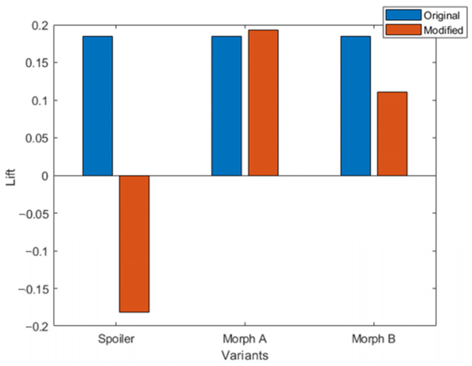
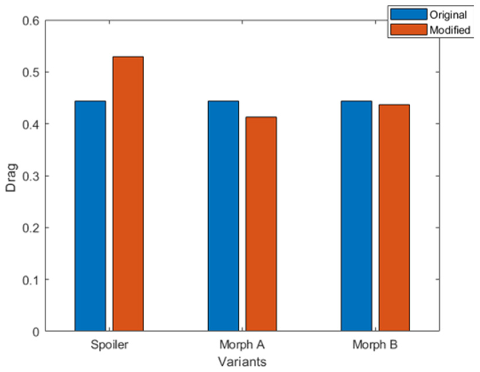
The primary objective of this study is to minimize aerodynamic drag and lift generation in order to improve the vehicle’s efficiency and stability. This was achieved using a NURBS-based morphing methodology, which allows for precise, localized shape refinements while maintaining global surface continuity (Figure 29 and Figure 30).

To ensure a fair evaluation, all simulations’ baseline and morphed variants were conducted under identical computational conditions (same mesh resolution, inlet velocity, turbulence model, and boundary conditions). This guarantees that observed differences in aerodynamic performance stem solely from geometric modifications introduced by the morphing process (

Table 3. Variant’s drag coefficient, lift coefficient, and percentage reduction from baseline.

V.No	Model	Cd	Cl	Cd Reducing (%)	Cl Reducing (%)
1	Baseline	0.443415	0.184196	-	-
2	Spoiler	0.529347	−0.182030	+19.38	−198.84
3	Morph A	0.412729	0.193074	−6.92	+4.82
4	Morph B	0.445455	0.110303	+0.46	−40.13

).

The original model serves as the reference dataset, representing the unmodified geometry with well-established aerodynamic behavior for similar coupe-class vehicles in the literature (Cd ≈ 0.44–0.46) [38]. Compared to the baseline, Morph A achieves a 6.9% reduction in Cd (from 0.4434 to 0.4127) with a marginal increase in Cl, while Morph B maintains a Cd comparable to the baseline but reduces Cl by 40.1% (from 0.1842 to 0.1103), thereby improving aerodynamic stability. These results highlight the targeted optimization effect of NURBS morphing: Morph A prioritizes drag reduction, whereas Morph B focuses on lift suppression.

Compared to other optimization methods, NURBS morphing provides designers with direct, smooth, and CAD-compatible control over vehicle geometry, allowing targeted aerodynamic refinements while preserving styling intent and manufacturability. Unlike mesh-based [39] or adjoint-driven approaches [40], it avoids producing irregular shapes that require extensive post-processing, enabling faster design iterations under consistent computational conditions [41,42]. While it may explore a smaller design space than fully automated optimization [43], its seamless integration into existing CAD workflows makes it a practical, designer-friendly tool that can be effectively combined with more data-driven methods for guided shape refinement.

5. Conclusions

This study focused on enhancing the aerodynamic performance of a sports car through morphing NURBS-based optimization, with all evaluations and comparative analyses carried out in the vehicle’s symmetry plane. By applying controlled, smooth geometric modifications to the rear-end and spoiler regions, the proposed approach preserved bilateral balance and enabled consistent comparison across design variants.

The CFD simulations, conducted in ANSYS Fluent using the RANS framework with the standard k-ε turbulence model, provided reliable predictions of boundary-layer development, wake dynamics, and flow separation. Among the configurations tested, the baseline geometry, a spoiler-equipped version, and two NURBS-morphed variants, Morph B emerged as the most effective, offering a significant reduction in lift, improved aerodynamic stability, and a favorable drag-to-lift ratio.

The integration of symmetry-plane performance evaluation with the flexibility of NURBS morphing proved to be a robust and adaptable methodology for aerodynamic optimization. Future developments could explore dynamic morphing strategies, additional aerodynamic devices, and multi-objective optimization frameworks to further exploit the benefits of symmetry and geometry control in automotive design.

Looking ahead, this approach could be expanded through multi-objective optimization to balance aerodynamic performance with structural, manufacturing, and weight constraints. Incorporating advanced turbulence models, transient flow simulations, and experimental validation would further improve accuracy. Exploring adaptive morphing systems that respond dynamically to driving conditions could also unlock intelligent, symmetry-preserving aerodynamic control in future vehicle designs.

References

1. Aerodynamics. Nature 1958, 181, 671–672. [CrossRef]
2. Lyu, Z.; Martins, J.R.R.A. Aerodynamic Design Optimization Studies of a Blended-Wing-Body Aircraft. J. Aircr. 2014, 51, 1604–1617. [Google Scholar] [CrossRef]
3. Firoozi, A.A.; Hejazi, F. Advancing Wind Energy Efficiency: A Systematic Review of Aerodynamic Optimization in Wind Turbine Blade Design. Energies 2024, 17, 2919. [Google Scholar] [CrossRef]
4. Thangadurai, M.; Kumar, R.; Rana, S.C.; Chatterjee, D. Aerodynamic Influence of Added Surfaces on the Performance Characteristics of a Sports Car. J. Inst. Eng. India Ser. C 2019, 100, 411–421. [Google Scholar] [CrossRef]
5. Hiemstra, R.R.; Shepherd, K.M.; Johnson, M.J.; Quan, L.; Hughes, T.J.R. Towards untrimmed NURBS: CAD embedded reparameterization of trimmed B-rep geometry using frame-field guided global parameterization. Comput. Methods Appl. Mech. Eng. 2020, 369, 113227. [Google Scholar] [CrossRef]
6. Gao, J.; Xiao, M.; Zhou, M.; Gao, L. Isogeometric topology and shape optimization for composite structures using level-sets and adaptive Gauss quadrature. Compos. Struct. 2022, 285, 115263. [Google Scholar] [CrossRef]
7. Thunich, P.; Tong, Y.; Müller, M. Efficient modelling of thermo-hydrodynamic properties in lubricated technical systems using NURBS-based isogeometric analysis. Tribol. Int. 2024, 199, 109934. [Google Scholar] [CrossRef]
8. Sarkar, S.; Thummar, K.; Shah, N.; Vagrecha, V. A Review paper on Aerodynamic Drag Reduction and CFD Analysis of Vehicles. Int. J. Progress. Res. Eng. Manag. Sci. 2019, 6. [Google Scholar]
9. Josefsson, E.; Hobeika, T.; Sebben, S. Evaluation of wind tunnel interference on numerical prediction of wheel aerodynamics. J. Wind Eng. Ind. Aerodyn. 2022, 224, 104945. [Google Scholar] [CrossRef]
10. Guendaoui, S.; Ouadefli, L.E.; El Akkad, A.; Elkhalfi, A.; Vlase, S.; Scutaru, M.L. Comparative Analysis of NURBS and Finite Element Method in Computational Fluid Dynamics Applications: Case Study on NACA 2412 Airfoil Aerodynamics. Mathematics 2024, 12, 3211. [Google Scholar] [CrossRef]
11. Goel, M.; Sharma, R.; Bhattacharyya, S.K.; Kim, T. NON-UNIFORM RATIONAL B-SPLINE BASED ISO-GEOMETRIC ANALYSIS FOR A CLASS OF HYDRODYNAMIC PROBLEMS. Int. J. Marit. Eng. 2020, 162. [Google Scholar] [CrossRef]
12. Zheng, R.; Kim, C. An Enhanced Topology Optimization Approach Based on the Combined MMC and NURBS-Curve Boundaries. Int. J. Precis. Eng. Manuf. 2020, 21, 1529–1538. [Google Scholar] [CrossRef]
13. Malik, F.E.; Mohammed, A.E.; Elhadi, I.D.; Al Hussein, M.S. CFD analysis and aerodynamic effects of add-on devices on an audi TT vehicle model. JME 2024, 14, 1. [Google Scholar] [CrossRef]
14. Launder, B.E.; Spalding, D.B. The numerical computation of turbulent flows. Comput. Methods Appl. Mech. Eng. 1974, 3, 269–289. [Google Scholar] [CrossRef]
15. Adriaenssens, S.; Block, P.; Veenendaal, D.; Williams, C. (Eds.) Shell Structures for Architecture; Routledge: Oxford, UK, 2014. [Google Scholar] [CrossRef]
16. Hughes, T.J.R.; Cottrell, J.A.; Bazilevs, Y. Isogeometric analysis: CAD, finite elements, NURBS, exact geometry and mesh refinement. Comput. Methods Appl. Mech. Eng. 2005, 194, 4135–4195. [Google Scholar] [CrossRef]
17. Cottrell, J.A.; Hughes, T.J.R.; Bazilevs, Y. Isogeometric Analysis: Toward Integration of CAD and FEA; John Wiley & Sons: Hoboken, NJ, USA, 2009. [Google Scholar]
18. Nouri, B.; Juhász, I.; Saeidian, J. A polynomial basis with a shape parameter for curve and surface modeling. Math. Comput. Simul. 2025, 229, 690–705. [Google Scholar] [CrossRef]
19. Chudy, F.; Woźny, P. Efficient evaluation of Bernstein-Bézier coefficients of B-spline basis functions over one knot span 2024. arXiv 2024, arXiv:2404.10396. [Google Scholar]
20. Laín, S.; Taborda, M.A.; López, O.D. Numerical Study of the Effect of Winglets on the Performance of a Straight Blade Darrieus Water Turbine. Energies 2018, 11, 297. [Google Scholar] [CrossRef]
21. Dornisch, W.; Stöckler, J.; Müller, R. Dual and approximate dual basis functions for B-splines and NURBS—Comparison and application for an efficient coupling of patches with the isogeometric mortar method. Comput. Methods Appl. Mech. Eng. 2017, 316, 449–496. [Google Scholar] [CrossRef]
22. Bidnichenko, H. Featured of Geometric Surfaces and Methods of their Computer Modeling. AGEG 2022, 102, 13–26. [Google Scholar] [CrossRef]
23. Eivazi, H.; Tahani, M.; Schlatter, P.; Vinuesa, R. Physics-informed neural networks for solving Reynolds-averaged Navier–Stokes equations. Phys. Fluids 2022, 34, 075117. [Google Scholar] [CrossRef]
24. Launder, B.E.; Spalding, D.B. Mathematical Models of Turbulence; Academic Press: London, UK; New York, NY, USA, 1972. [Google Scholar]
25. Renold Elsen, S.; Jegadeesan, K.; Ronald Aseer, J. A Comparative Study of Flow Characteristics of BMW M6 and AUDI R8 Commercial Sports Car Using Flow Design Software. In Advances in Manufacturing Technology; Hiremath, S.S., Shanmugam, N.S., Bapu, B.R.R., Eds.; Lecture Notes in Mechanical Engineering; Springer: Singapore, 2019; pp. 243–253. [Google Scholar] [CrossRef]
26. Elrefaie, M.; Dai, A.; Ahmed, F. DrivAerNet: A Parametric Car Dataset for Data-Driven Aerodynamic Design and Prediction. In Proceedings of the Volume 3A: 50th Design Automation Conference (DAC), Washington, DC, USA, 25–28 August 2024; p. V03AT03A019. [Google Scholar] [CrossRef]
27. Yu, P.X.; Tian, Z.F. An upwind compact difference scheme for solving the streamfunction–velocity formulation of the unsteady incompressible Navier–Stokes equation. Comput. Math. Appl. 2018, 75, 3224–3243. [Google Scholar] [CrossRef]
28. Patel, A.; Boersma, B.J.; Pecnik, R. The influence of near-wall density and viscosity gradients on turbulence in channel flows. J. Fluid Mech. 2016, 809, 793–820. [Google Scholar] [CrossRef]
29. Cavar, D.; Réthoré, P.-E.; Bechmann, A.; Sørensen, N.N.; Martinez, B.; Zahle, F.; Berg, J.; Kelly, M.C. Comparison of OpenFOAM and EllipSys3D for neutral atmospheric flow over complex terrain. Wind Energy Sci. 2016, 1, 55–70. [Google Scholar] [CrossRef]
30. Sarjito, S.; Junaidin, B.; Wijayanto, B. Modification of Drag and Lift Balance at Analog Wind Tunnel for Identification of Aerodynamic Performance. In Proceedings of the 6th International Conference on Advanced Materials Science, Surakarta, Indonesia, 23–24 August 2024; pp. 113–118. [Google Scholar] [CrossRef]
31. Eftekhari, H.; Al-Obaidi, A.S.M.; Eftekhari, S. The Effect of Spoiler Shape and Setting Angle on Racing Cars Aerodynamic Performance. Indones. J. Sci. Technol. 2020, 5, 11–20. [Google Scholar] [CrossRef]
32. Magalhães Júnior, J.M.; Halila, G.L.O.; Kim, Y.; Khamvilai, T.; Vamvoudakis, K.G. Intelligent data-driven aerodynamic analysis and optimization of morphing configurations. Aerosp. Sci. Technol. 2022, 121, 107388. [Google Scholar] [CrossRef]
33. Qin, P.; Ricci, A.; Blocken, B. CFD simulation of aerodynamic forces on the DrivAer car model: Impact of computational parameters. J. Wind Eng. Ind. Aerodyn. 2024, 248, 105711. [Google Scholar] [CrossRef]
34. Bauer, A.; Breitenberger, M.; Philipp, B.; Wüchner, R.; Bletzinger, K.-U. Embedded structural entities in NURBS-based isogeometric analysis. Comput. Methods Appl. Mech. Eng. 2017, 325, 198–218. [Google Scholar] [CrossRef]
35. Hui, X.; Bai, J.; Wang, H.; Zhang, Y. Fast pressure distribution prediction of airfoils using deep learning. Aerosp. Sci. Technol. 2020, 105, 105949. [Google Scholar] [CrossRef]
36. Das, R.; Girimaji, S. Characterization of velocity-gradient dynamics in incompressible turbulence using local streamline geometry. J. Fluid Mech. 2020, 895. [Google Scholar] [CrossRef]
37. Menter, F.; Kuntz, M. Adaptation of Eddy-Viscosity Turbulence Models to Unsteady Separated Flow Behind Vehicles. In The Aerodynamics of Heavy Vehicles: Trucks, Buses, and Trains; Springer: Berlin/Heidelberg, Germany, 2004. [Google Scholar] [CrossRef]
38. Nath, D.; Pujari, P.; Jain, A.; Rastogi, V. Drag reduction by application of aerodynamic devices in a race car. Adv. Aerodyn. 2021, 3, 4. [Google Scholar] [CrossRef]
39. Chen, G.; Fidkowski, K. Variable-fidelity multipoint aerodynamic shape optimization with output-based adapted meshes. Aerosp. Sci. Technol. 2020, 105, 106004. [Google Scholar] [CrossRef]
40. He, P.; Mader, C.; Martins, J.; Maki, K. An aerodynamic design optimization framework using a discrete adjoint approach with OpenFOAM. Comput. Fluids 2018, 168, 285–303. [Google Scholar] [CrossRef]
41. El-Mekkaoui, J.; Elkhalfi, A.; Elakkad, A. Resolution of stokes equations with the Ca,b boundary condition using mixed finite element method. WSEAS Trans. Math. 2013, 12, 586–597. [Google Scholar]
42. El Fakkoussi, S.; Moustabchir, H.; Elkhalfi, A.; Pruncu, C.I. Application of the extended isogeometric analysis (X-IGA) to evaluate a pipeline structure containing an external crack. J. Eng. 2018, 2018, 4125765. [Google Scholar] [CrossRef]
43. El Barkany, A.; Abdelouahhab, J.; El Khalfi, A. Optimizing the integrated production and maintenance planning using genetic algorithm. Int. J. Eng. Bus. Manag. 2018, 102018, 1–9. [Google Scholar] [CrossRef]
Figure 1. Geometric descriptions showing a NURBS refinement on the left and a polygonal mesh.
Symmetry 17 01571 g001
Figure 2. Degree elevation from 1 to 4 for an identical set of control points.
Symmetry 17 01571 g002
Figure 3. Example of basis functions for one single knot span (two, three, four, five basis functions) [19].
Symmetry 17 01571 g003
Figure 4. (Right) NURBS with weights describes perfect quarter circle. (Left) B-spline with constant weights.
Symmetry 17 01571 g004
Figure 5. Geometry of an arbitrary shell body.
Symmetry 17 01571 g005
Figure 6. The 3D model of the original geometry created using blueprint method in CATIA V5.
Symmetry 17 01571 g006
Figure 7. Domain and boundary conditions’ representation.
Symmetry 17 01571 g007
Figure 8. Snappy-Hex-Mesh (SHM) and mesh refinement.
Symmetry 17 01571 g008
Figure 9. The convergence histories of the drag and lift coefficients for the original geometry.
Symmetry 17 01571 g009
Figure 10. Streamlines of the original geometry in the symmetry plane. The same color is for the same velocity of the air.
Symmetry 17 01571 g010
Figure 11. Spoiler cross-section selection using airfoil-tool database.
Symmetry 17 01571 g011
Figure 12. The convergence histories of the drag coefficients for the vehicle with spoiler geometry.
Symmetry 17 01571 g012
Figure 13. The convergence histories of the lift coefficients for the vehicle with spoiler geometry.
Symmetry 17 01571 g013
Figure 14. The pressure contour distribution of the spoiler variant.
Symmetry 17 01571 g014
Figure 15. Streamlines of the spoiler variant geometry in the symmetry plane. The particle of air having the same velocity have the same colour.
Symmetry 17 01571 g015
Figure 16. Parameters impacting the aerodynamic vehicle performance. With red are represented the horizontal and vertical axis.
Symmetry 17 01571 g016
Figure 17. Morph A modified Variant geometry optimization using NURBS control boxes.
Symmetry 17 01571 g017
Figure 18. Morph B Variant geometry optimization using NURBS control boxes.
Symmetry 17 01571 g018
Figure 19. Drag convergence of Variant Morph A.
Symmetry 17 01571 g019
Figure 20. Lift convergence of Variant Morph A.
Symmetry 17 01571 g020
Figure 21. Drag convergence Variant Morph B.
Symmetry 17 01571 g021
Figure 22. Lift convergence Variant Morph B.
Symmetry 17 01571 g022
Figure 23. The surface pressure distribution over the Morph A Variant.
Symmetry 17 01571 g023
Figure 24. The surface pressure distribution over the Morph B Variant.
Symmetry 17 01571 g024
Figure 25. Z = 6, Z = 10 and Z = 11 axis control position in the symmetry plane of the computational domain.
Symmetry 17 01571 g025
Figure 26. Comparison of aerodynamic variables for car variants at Z = 6 m control axis.
Symmetry 17 01571 g026
Figure 27. Comparison of aerodynamic variables for car variants at Z = 10 m control axis.
Symmetry 17 01571 g027
Figure 28. Comparison of aerodynamic variables for car variants at Z = 11 m control axis.
Symmetry 17 01571 g028
Figure 29. Lift coefficient of the modified variants compared to the original design.
Symmetry 17 01571 g029
Figure 30. Drag coefficient of the modified variants compared to the original design.
Symmetry 17 01571 g030