Article

Combining Constructed Artificial Neural Networks with Parameter Constraint Techniques to Achieve Better Generalization Properties

by
Ioannis G. Tsoulos
1,*,
Vasileios Charilogis
1 and
Dimitrios Tsalikakis
2
1
Department of Informatics and Telecommunications, University of Ioannina, 45110 Ioannina, Greece
2
Department of Engineering Informatics and Telecommunications, University of Western Macedonia, 50100 Kozani, Greece
*
Author to whom correspondence should be addressed.
Symmetry 2025, 17(9), 1557; https://doi.org/10.3390/sym17091557
Submission received: 27 August 2025 / Revised: 7 September 2025 / Accepted: 9 September 2025 / Published: 17 September 2025

Abstract

This study presents a novel hybrid approach combining grammatical evolution with constrained genetic algorithms to overcome key limitations in automated neural network design. The proposed method addresses two critical challenges: the tendency of grammatical evolution to converge to suboptimal architectures due to local optima, and the common overfitting problems in evolved networks. Our solution employs grammatical evolution for initial architecture generation while implementing a specialized genetic algorithm that simultaneously optimizes network parameters within dynamically adjusted bounds. The genetic component incorporates innovative penalty mechanisms in its fitness function to control neuron activation patterns and prevent overfitting. Comprehensive testing across 53 diverse datasets shows our method achieves superior performance compared to traditional optimization techniques, with an average classification error of 21.18% vs. 36.45% for ADAM, while maintaining better generalization capabilities. The constrained optimization approach proves particularly effective in preventing premature convergence, and the penalty system successfully mitigates overfitting even in complex, high-dimensional problems. Statistical validation confirms these improvements are significant (p < 1.1 × 10 8 ) and consistent across multiple domains, including medical diagnosis, financial prediction, and physical system modeling. This work provides a robust framework for automated neural network construction that balances architectural innovation with parameter optimization while addressing fundamental challenges in evolutionary machine learning.

1. Introduction

A basic machine learning technique with a wide range of applications in data classification and regression problems is artificial neural networks [1,2]. Artificial neural networks are parametric machine learning models, in which learning is achieved by effectively adjusting their parameters through any optimization technique. The optimization procedure minimizes the so-called training error of an artificial neural network, and it is defined as
E N x , w = i = 1 M N x i , w y i 2
In this equation, the function N x , w represents the artificial neural network that is applied to a vector x , and the vector w denotes the parameter vector of the neural network. The set x i , y i , i = 1 , , M represents the training set of the objective problem, and the values y i are the expected outputs for each pattern x i .
Artificial neural networks have been applied in a wide series of real-world problems, such as image processing [3], time series forecasting [4], credit card analysis [5], problems derived from physics [6], etc. Also, a series of studies were published related to the correlation of symmetry and artificial neural networks, such as the work of Aguirre et al. [7], where neural networks were trained using data produced by systems with symmetry properties. Furthermore, Mattheakis et al. [8] discussed the application of physical constraints to the structure of neural networks to maintain some basic symmetries in their design. Moreover, Krippendorf et al. [9] proposed a method that identify symmetries in datasets using neural networks.
Due to the widespread use of these machine learning models, a number of techniques have been proposed to minimize Equation (1), such as the back propagation algorithm [10], the RPROP algorithm [11,12], the ADAM optimization method [13], etc. Recently, a series of more advanced global optimization methods were proposed to tackle the training of neural networks. Among them, one can locate the incorporation of genetic algorithms [14], the usage of the particle swarm optimization (PSO) method [15], the simulated annealing method [16], the differential evolution technique [17], the artificial bee colony (ABC) method [18], etc. Furthermore, Sexton et al suggested the usage of the tabu search algorithm for optimal neural network training [19], and Zhang et al. proposed a hybrid algorithm that incorporated the PSO method and the back propagation algorithm to efficiently train artificial neural networks [20]. Also, recently, Zhao et al. introduced a new cascaded forward algorithm to train artificial neural networks [21]. Furthermore, due to the rapid spread of the use of parallel computing techniques, a series of computational techniques have emerged that exploit parallel computing structures for faster training of artificial neural networks [22,23].
However, the above techniques, although extremely effective, nevertheless have a number of problems, such as, for example, trapping in local minima of the error function or the phenomenon of overifitting, where the artificial neural network exhibits reduced performance when applied to data that was not present during the training process. The overfitting problem has been studied by many researchers that have proposed a series of methods to handle this problem, such as weight sharing [24,25], pruning [26,27], early stopping [28,29], weight decaying [30,31], etc. Also, many researchers have proposed as a solution to the above problem the dynamic creation of the architecture of artificial neural networks using programming techniques. For example, genetic algorithms were proposed to dynamically create the optimal architecture of neural networks [32,33] or the PSO method [34]. Siebel et al. suggested the usage of evolutionary reinforcement learning for the optimal design of artificial neural networks [35]. Also, Jaafra et al. provided a review on the usage of reinforcement learning for neural architecture search [36]. In the same direction of research, Pham et al. proposed a method for efficient identification of the architecture of neural networks through parameters sharing [37]. Also, the method of stochastic neural architecture search was suggested by Xie et al. in a recent publication [38]. Moreover, Zhou et al. introduced a Bayesian approach for neural architecture search [39].
Recently, genetic algorithms have been incorporated to identify the optimal set of parameters of neural networks for drug discovery [40]. Kim et al. proposed [41] genetic algorithms to train neural networks for predicting preliminary cost estimates. Moreover, Kalogirou proposed the usage of genetic algorithms for effective training of neural networks for the optimization of solar systems [42]. The ability of neural networks to perform feature selection with the assistance of genetic algorithms was also studied in the work of Tong et al. [43]. Recently, Ruehle provided a study of the string landscape using genetic algorithms to train artificial neural networks [44]. Genetic algorithms have also been used in variety of symmetry problems from the relevant literature [45,46,47].
A method that was proposed relatively recently, based on grammatical evolution [48], dynamically identifies both the optimal architecture of artificial neural networks and the optimal values of its parameters [49]. This method has been applied in a series of problems in the recent literature, such as problems presented in chemistry [50], identification of the solution of differential equations [51], medical problems [52], problems related to education [53], autism screening [54], etc. A key advantage of this technique is that it can isolate from the initial features of the problem those that are most important in training the model, thus significantly reducing the required number of parameters that need to be identified.
However, the method of constructing artificial neural networks can easily get trapped in local minima of the training error since it does not have any technique to avoid them. Furthermore, although the method can get quite close to a minimum of the training error, it often does not reach it since there is no technique in the method to train the generated parameters. In this technique, it is proposed to enhance the original method of constructing artificial neural networks by periodically applying a modified genetic algorithm to randomly selected chromosomes of grammatical evolution. This modified genetic algorithm preserves the architecture created by the grammatical evolution method and effectively locates the parameters of the artificial neural network by reducing the training error. In addition, the proposed genetic algorithm through appropriate penalty factors imposed on the fitness function prevents the artificial neural network from overfitting.
The motivation of the proposed method is the need to address two main challenges in training artificial neural networks: getting trapped in local minima and the phenomenon of overfitting. Getting trapped in local minima limits the model’s ability to minimize training error, leading to poor performance on test data. Overfitting similarly reduces generalization, as the model adapts excessively to the training data. The proposed method combines grammatical evolution with a modified genetic algorithm to address these problems. Grammatical evolution is used for the dynamic construction of the neural network’s architecture, while the genetic algorithm optimizes the network’s parameters while preserving its structure. Additionally, penalty factors are introduced in the cost function to prevent overfitting. A key innovation is the use of an algorithm that measures the network’s tendency to lose generalization capability when neuron activations become saturated. This is achieved by monitoring the input values of the sigmoid function and imposing penalties when they exceed a specified range. Experimental tests showed that the method outperforms other techniques, such as ADAM, BFGS, and RBF networks, in both classification and regression problems. Statistical analysis confirmed the significant improvement in performance, with very low p-values in the comparisons.
For the suggested work, the main contributions are as follows:
1.
A novel hybrid framework that effectively combines grammatical evolution for neural architecture search with constrained genetic algorithms for parameter optimization, addressing both structural design and weight training simultaneously;
2.
An innovative penalty mechanism within the genetic algorithm’s fitness function that dynamically monitors and controls neuron activation patterns to prevent overfitting, demonstrated to reduce test error by an average of 15.27% compared to standard approaches;
3.
Comprehensive experimental validation across 53 diverse datasets showing statistically significant improvements ( p < 1.1 × 10 8 ) over traditional optimization methods, with particular effectiveness in medical and financial domains where overfitting risks are critical;
4.
Detailed analysis of the method’s computational characteristics and scalability, providing practical guidelines for implementation in real-world scenarios with resource constraints.
Although the method can construct the correct network structure, its parameters often remain suboptimal. This means the network fails to fully exploit its architecture’s potential, resulting in lower performance compared to other approaches. Furthermore, the absence of efficient training mechanisms leads to increased training times, making the method less practical for applications requiring quick results. In specific application scenarios, these limitations become even more apparent. For instance, with high-dimensional data, the method struggles to identify relationships between features while computational times become prohibitive. With limited training data, the constructed networks tend to overfit, resulting in poor generalization to new data. For real-time applications, the high computational complexity makes the method impractical. Compared to other approaches like traditional neural networks with backpropagation, modern deep learning architectures, or meta-learning methods, grammatical evolution appears inferior in several aspects. It requires significantly more computational resources, consistently achieves lower performance, and presents scalability limitations. These factors restrict the method’s application in production systems where stability and result predictability are crucial. The practical implications of these limitations are substantial. The method requires extensive hyperparameter tuning to produce acceptable results, while its performance can be unpredictable and vary significantly between different runs. For successful application to real-world problems, additional processing and result validation are often necessary. Despite its limitations, the method offers interesting capabilities for the automatic construction of neural network architectures. However, to become truly competitive against existing approaches, it requires the development of more sophisticated optimization algorithms to reduce local minima trapping, the integration of efficient parameter training mechanisms, and improvements in method scalability. Only by addressing these issues can grammatical evolution emerge as an attractive alternative in the field of automated neural network design.
The main contributions of the proposed work can be summarized as follows:
1.
Periodic application of an optimization technique to randomly selected chromosomes with the aim of improving the performance of the selected neural network but also of faster finding the global minimum of the error function;
2.
The training of the artificial neural network by the optimization method is done in such a way as not to destroy the architecture of the neural network that grammatical evolution has already constructed;
3.
The training of the artificial neural network from the optimization function is carried out using a modified fitness function, where an attempt is made to adapt the network parameters without losing its generalization properties.
The remainder of this article is organized as follows: in Section 2, the proposed method and the accompanied genetic algorithm are introduced; in Section 3, the experimental datasets and the series of experiments conducted are listed and discussed thoroughly; in Section 4, a discussion on the experimental results is provided; and, finally, in Section 5, some conclusions are discussed.

2. Method Description

This section provides a detailed description of the original neural network construction method, continues with the proposed genetic algorithm, and concludes with the overall algorithm.

2.1. The Neural Construction Method

The neural construction method utilizes the technique of grammatical evolution to produce artificial neural networks. Grammatical evolution is an evolutionary process where the chromosomes are vectors of positive integers. These integers represent rules from a Backus–Naur form (BNF) grammar [55] of the target language. The method was incorporated in various cases, such as data fitting [56,57], composition of music [58], video games [59,60], energy problems [61], cryptography [62], economics [63], etc. Any BNF grammar is defined as a set G = N , T , S , P where the letters have the following definitions:
  • The set N represents the non-terminal symbols of the grammar.
  • The set T contains the terminal symbols of the grammar.
  • The start symbol of the grammar is denoted as S.
  • The production rules of the grammar are enclosed in the set P.
The grammatical evolution production procedure initiates from the starting symbol S and, following a series of steps, the method creates valid programs by replacing non-terminal symbols with the right hand of the selected production rule. The selection scheme has
  • Read the next element V from the chromosome that is being processed;
  • Select the next production rule following the equation: Rule = V mod N R . The symbol N R represents the total number of production rules for the under processing non-terminal symbol.
The process of producing valid programs through the grammatical evolution method is depicted graphically in Figure 1.
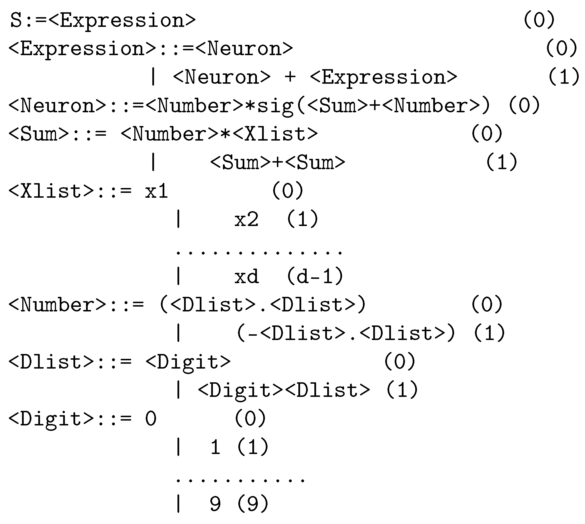
The grammar used for the neural construction procedure is shown in Figure 2. The numbers shown in parentheses are the increasing numbers of the production rules for each non-terminal symbol. The constant d denotes the number of features in every pattern of the input dataset.
The used grammar produces artificial neural networks with the following form:
N x , w = i = 1 H w ( d + 2 ) i ( d + 1 ) σ j = 1 d x j w ( d + 2 ) i ( d + 1 ) + j + w ( d + 2 ) i
The term H stands for the number of processing units (weights) of the neural network. The function σ ( x ) represents the sigmoid function. The total number of parameters for this network are computed through the following equation:
n = d + 2 H
For example, the following form
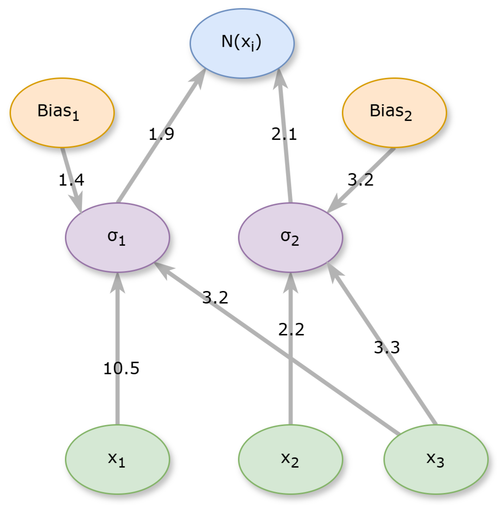
N ( x ) = 1.9 s i g 10.5 x 1 + 3.2 x 3 + 1.4 + 2.1 s i g 2.2 x 2 3.3 x 3 + 3.2
denotes a produced neural network for a problem with three inputs, x 1 , x 2 , x 3 and the number of processing nodes is H = 2 . The neural network produced is shown graphically in Figure 3.

2.2. The Used Genetic Algorithm

It is proposed in this work to introduce the concept of local search through the periodic application of a genetic algorithm that should maintain the structure of the neural network constructed by the original method. Additionally, a second goal of this genetic algorithm should be to avoid the problem of overfitting that could arise from simply applying a local optimization method to the previous artificial neural network. For the first goal of the modified genetic algorithm, consider the example neural network shown before:
N ( x ) = 1.9 sig 10.5 x 1 + 3.2 x 3 + 1.4 + 2.1 s i g 2.2 x 2 3.3 x 3 + 3.2
The weight vector w for this neural network is
w = 1.9 , 10.5 , 0.0 , 3.2 , 1.4 , 2.1 , 0.0 , 2.2 , 3.3 , 3.2
In order to protect the structure of this artificial neural network, the modified genetic algorithm should allow changes in the parameters of this network within a value interval, which can be considered to be the pair of vectors L , R . The elements for the vector L are defined as
L i = F × w i , i = 1 , , n
where F is positive number with F > 1 . Likewise, the right bound for the parameters R is defined from the following equation:
R i = F × w i , i = 1 , , n
For the example weight vector of Equation (6) and for F = 2 , the following vectors are used:
L = 3.8 , 21.0 , 0.0 , 6.4 , 2.8 , 4.2 , 0.0 , 4.4 , 6.6 , 6.4 R = 3.8 , 21.0 , 0.0 , 6.4 , 2.8 , 4.2 , 0.0 , 4.4 , 6.6 , 6.4
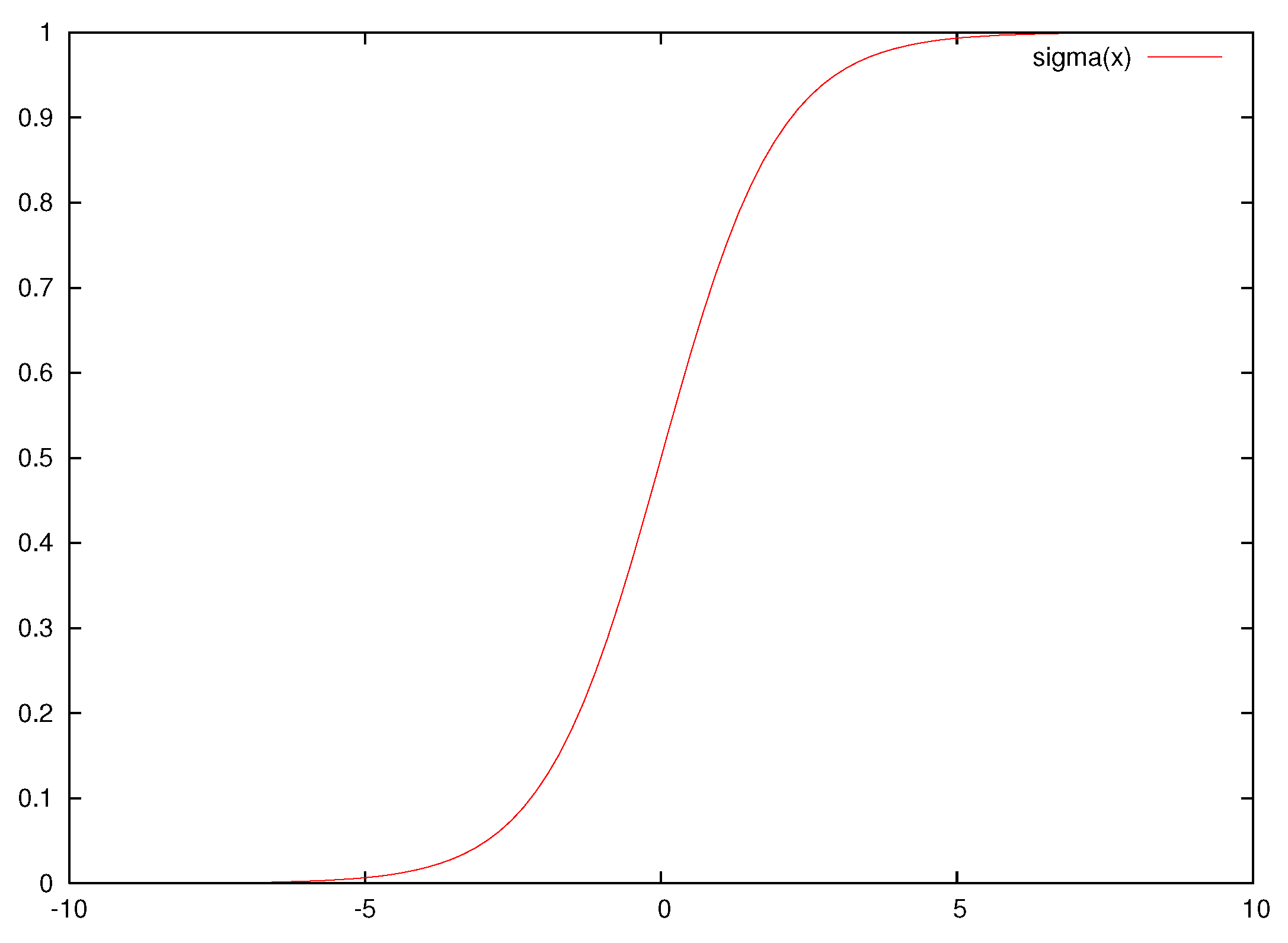
The modified genetic algorithm should also prevent the artificial neural networks it trains from the phenomenon of overfitting, which would lead to poor results on the test dataset. For this reason, a quantity derived from the publication of Anastasopoulos et al. [64] is utilized here. The sigmoid function, which is used as the activation function of neural networks, is defined as
σ ( x ) = 1 1 + exp ( x )
A plot for this function is shown in Figure 4.
As is clear from the equation and the figure, as the value of the parameter x increases, the function tends very quickly to 1. On the other hand, the function will take values very close to 0 as the parameter x decreases. This means that the function very quickly loses the generalizing abilities it has and therefore large changes in the value of the parameter x will not cause proportional variations in the value of the sigmoid function. Therefore, the quantity B N x , w , a was introduced in that paper to measure this effect. This quantity is calculated through the process of Algorithm 1. This function may be used to avoid overfitting by limiting the parameters of the neural network to intervals that depend on the objective problem. The user defined parameter a is used here as a limit for the input value of the sigmoid unit. If this value exceeds a, then the neural network probably has a reduced generalization ability, since the sigmoid output will be the same regardless of any change in the input value.
Algorithm 1 The algorithm used to calculate the bounding quantity for neural network N ( x , w ) .
function  evalB N x , w , a
1.
Inputs: The neural network N x , w and the double precision value a , a > 1 .
2.
Set  s = 0
3.
For  i = 1 . . H  Do
(a)
For  j = 1 . . M  Do
i.
Calculate  v = k T = 1 d w ( d + 2 ) i ( d + i ) + k x j k + w ( d + 2 ) i
ii.
If  v > a  set  s = s + 1
(b)
End For
4.
End For
5.
Return s H M
End Function
The overall proposed modified genetic algorithm is shown in Algorithm 2.
Algorithm 2 The modified genetic algorithm.
Function  mGA L , R , a , λ
1.
Inputs: The bound vectors L , R and the bounding factor a and λ a positive value with λ > 1 .
2.
Set as N K the number of allowed generations and as N G the number of used chromosomes.
3.
Set as p S the selection rate and as p M the mutation rate.
4.
Initialize  N G chromosomes inside the bounding boxes L , R .
5.
Set  k = 0 , the generation number.
6.
For  i = 1 , , N G
(a)
Obtain the corresponding neural network N i x , g i for the chromosome g i .
(b)
Set  e i = j = 1 M N i x j , w i y j 2
(c)
Set  B i = e v a l N i x , g i , a using the Algorithm 1.
(d)
Set  f i = e i × 1 + λ B i 2 as the fitness value of chromosome g i
7.
End For
8.
Select the best 1 p s × N G chromosomes, that will be copied intact to the next generation. The remaining will be substituted by individuals produced by crossover and mutation.
9.
Set  k = k + 1
10.
If  k N K  goto step 6.
End function

2.3. The Overall Algorithm

The overall algorithm uses the procedures presented previously to achieve greater accuracy in calculations as well as to avoid overfitting phenomena. The steps of the overall algorithm are as follows:
1.
Initialization.
(a)
Set as N C the number of chromosomes for the grammatical evolution procedure and as N G the maximum number of allowed generations.
(b)
Set as p S the selection rate and as p M the mutation rate.
(c)
Let  N I be the number of chromosomes to which the modified genetic algorithm will be periodically applied.
(d)
Let  N T be the number of generations that will pass before applying the modified genetic algorithm to randomly selected chromosomes.
(e)
Set the weight factor F with F > 1 .
(f)
Set the values N K , a , λ used in the modified genetic algorithm.
(g)
Initialize randomly the N C chromosomes as sets of randomly selected integers.
(h)
Set the generation number k = 0 .
2.
Fitness Calculation.
(a)
For  i = 1 , , N C  do
i.
Obtain the chromosome g i .
ii.
Create the corresponding neural network N i x , w using grammatical evolution.
iii.
Set the fitness value f i = j = 1 M N i x j , w y j 2 .
(b)
End For
3.
Genetic Operations.
(a)
Select the best 1 p s × N G chromosomes, which will be copied intact to the next generation.
(b)
Create  p S N chromosomes using one-point crossover. For every couple c 1 , c 2 of produced offspring two distinct chromosomes are selected from the current population using tournament selection. An example of the one-point crossover procedure is shown graphically in Figure 5.
(c)
For every chromosome and for each element select a random number r 1 . Alter the current element when r p M .
4.
Local Search.
(a)
If  k mod N T = 0  then
i.
Set  S = g r 1 , g r 2 , , g r N I a group of N I randomly selected chromosomes from the genetic population.
ii.
For every member g S  do
A.
Obtain the corresponding neural network N g x , w for the chromosome g.
B.
Create the left bound vector L g and the right bound vector R g for g using Equations (7) and (8), respectively.
C.
Set  g = m g a L g , R g , a , λ using the steps of Algorithm 2.
iii.
End For
(b)
Endif
5.
Termination Check.
(a)
Set  k = k + 1 .
(b)
If  k N G goto Fitness Calculation.
6.
Application to the Test Set.
(a)
Obtain the chromosome g * with the lowest fitness value and create through grammatical evolution the corresponding neural network N * x , w .
(b)
Apply the neural network N * x , w and report the corresponding error value.
Figure 5. An example of the one-point crossover procedure.The blue color denotes the elements of the first chromosome and the green color is used for the elements of the second chromosome.
Symmetry 17 01557 g005
The main steps of the overall algorithm are graphically illustrated in Figure 6.
Figure 6. The flowchart of the overall algorithm.
Symmetry 17 01557 g006

3. Experimental Results

The validation of the proposed method was performed using a wide series of classification and regression datasets, available from various sources on the Internet. These datasets were downloaded from:
1.
The UCI database, https://archive.ics.uci.edu/ (accessed on 22 January 2025) [65];
2.
The Keel website, https://sci2s.ugr.es/keel/datasets.php (accessed on 22 January 2025) [66];
3.
The Statlib URL https://lib.stat.cmu.edu/datasets/index (accessed on 22 January 2025).

3.1. Experimental Datasets

The following datasets were utilized in the conducted experiments:
1.
Appendictis which is a medical dataset [67];
2.
Alcohol, which is dataset regarding alcohol consumption [68];
3.
Australian, which is a dataset produced from various bank transactions [69];
4.
Balance dataset [70], produced from various psychological experiments;
5.
Cleveland, a medical dataset that was discussed in a series of papers [71,72];
6.
Circular dataset, which is an artificial dataset;
7.
Dermatology, a medical dataset for dermatology problems [73];
8.
Ecoli, which is related to protein problems [74];
9.
Glass dataset, which contains measurements from glass component analysis;
10.
Haberman, a medical dataset related to breast cancer;
11.
Hayes-roth dataset [75];
12.
Heart, which is a dataset related to heart diseases [76];
13.
HeartAttack, which is a medical dataset for the detection of heart diseases;
14.
Housevotes, a dataset that is related to the Congressional voting in the USA [77];
15.
Ionosphere, a dataset that contains measurements from the ionosphere [78,79];
16.
Liverdisorder, a medical dataset that was studied thoroughly in a series of papers [80,81];
17.
Lymography [82];
18.
Mammographic, which is a medical dataset used for the prediction of breast cancer [83];
19.
Parkinsons, which is a medical dataset used for the detection of Parkinson’s disease [84,85];
20.
Pima, which is a medical dataset for the detection of diabetes [86];
21.
Phoneme, a dataset that contains sound measurements;
22.
Popfailures, a dataset related to experiments regarding climate [87];
23.
Regions2, a medical dataset applied to liver problems [88];
24.
Saheart, which is a medical dataset concerning heart diseases [89];
25.
Segment dataset [90];
26.
Statheart, a medical dataset related to heart diseases;
27.
Spiral, an artificial dataset with two classes;
28.
Student, which is a dataset regarding experiments in schools [91];
29.
Transfusion, which is a medical dataset [92];
30.
Wdbc, which is a medical dataset regarding breast cancer [93,94];
31.
Wine, a dataset regarding measurements about the quality of wines [95,96];
32.
EEG, which is dataset regardingEEG recordings [97,98]. From this dataset, the following cases were used: Z_F_S, ZO_NF_S, ZONF_S and Z_O_N_F_S;
33.
Zoo, which is a dataset regarding animal classification [99].
Moreover, a series of regression datasets was adopted in the conducted experiments. The list with the regression datasets is as follows:
1.
Abalone, which is a dataset about the age of abalones [100];
2.
Airfoil, a dataset founded in NASA [101];
3.
Auto, a dataset related to the consumption of fuels from cars;
4.
BK, which is used to predict the points scored in basketball games;
5.
BL, a dataset that contains measurements from electricity experiments;
6.
Baseball, which is a dataset used to predict the income of baseball players;
7.
Concrete, which is a civil engineering dataset [102];
8.
DEE, a dataset that is used to predict the price of electricity;
9.
Friedman, which is an artificial dataset [103];
10.
FY, which is a dataset regarding the longevity of fruit flies;
11.
HO, a dataset located in the STATLIB repository;
12.
Housing, a dataset regarding the price of houses [104];
13.
Laser, which contains measurements from various physics experiments;
14.
LW, a dataset regarding the weight of babes;
15.
Mortgage, a dataset that contains measurements from the economy of the USA;
16.
PL dataset, located in the STALIB repository;
17.
Plastic, a dataset regarding problems that occurred with the pressure on plastics;
18.
Quake, a dataset regarding the measurements of earthquakes;
19.
SN, a dataset related to trellising and pruning;
20.
Stock, which is a dataset regarding stocks;
21.
Treasury, a dataset that contains measurements from the economy of the USA.

3.2. Experiments

The software used in the experiment was coded in C++ programming language with the assistance of the freely available Optimus environment [105]. Every experiment was conducted 30 times and each time a different seed for the random generator was used. The experiments were validated using the ten-fold cross-validation technique. The average classification error as measured in the corresponding test set was reported for the classification datasets. This error is calculated through the following formula:
E C N x , w = 100 × i = 1 N c l a s s N x i , w y i N
Here, the test set T is a set T = x i , y i , i = 1 , , N . Likewise, the average regression error is reported for the regression datasets. This error can be obtained using the following equation:
E R N x , w = i = 1 N N x i , w y i 2 N
The experiments were executed on an AMD Ryzen 5950X with 128 GB of RAM and the operating system used was Debian Linux (bookworm version). The values for the parameters of the proposed method are shown in Table 1.
The parameter values were chosen in such a way that there is a balance between the speed of the proposed method and its efficiency. In the following tables that describe the experimental results, the following notation is used:
1.
The column DATASET represents the used dataset.
2.
The column ADAM represents the incorporation of the ADAM optimization method [13] to train a neural network with H = 10 processing nodes.
3.
The column BFGS stands for the usage of a BFGS variant of Powell [106] to train an artificial neural network with H = 10 processing nodes.
4.
The column GENETIC represents the incorporation of a genetic algorithm with the same parameter set as provided in Table 1 to train a neural network with H = 10 processing nodes.
5.
The column RBF describes the experimental results obtained by the application of a radial basis function (RBF) network [107,108] with H = 10 hidden nodes.
6.
The column NNC stands for the usage of the original neural construction method.
7.
The column NEAT represents the usage of the NEAT method (neuroevolution of augmenting topologies) [109].
8.
The column PRUNE stands for the the usage of OBS pruning method [110], as coded in the Fast Compressed Neural Networks Library [111].
9.
The column DNN represents the application of the deep neural network provided in the Tiny Dnn library, which is available from https://github.com/tiny-dnn/tiny-dnn (accessed on 7 September 2025). The network was trained using the AdaGrad optimizer [112].
10.
The column PROPOSED denotes the usage of the proposed method.
11.
The row AVERAGE represents the average classification or regression error for all datasets in the corresponding table.
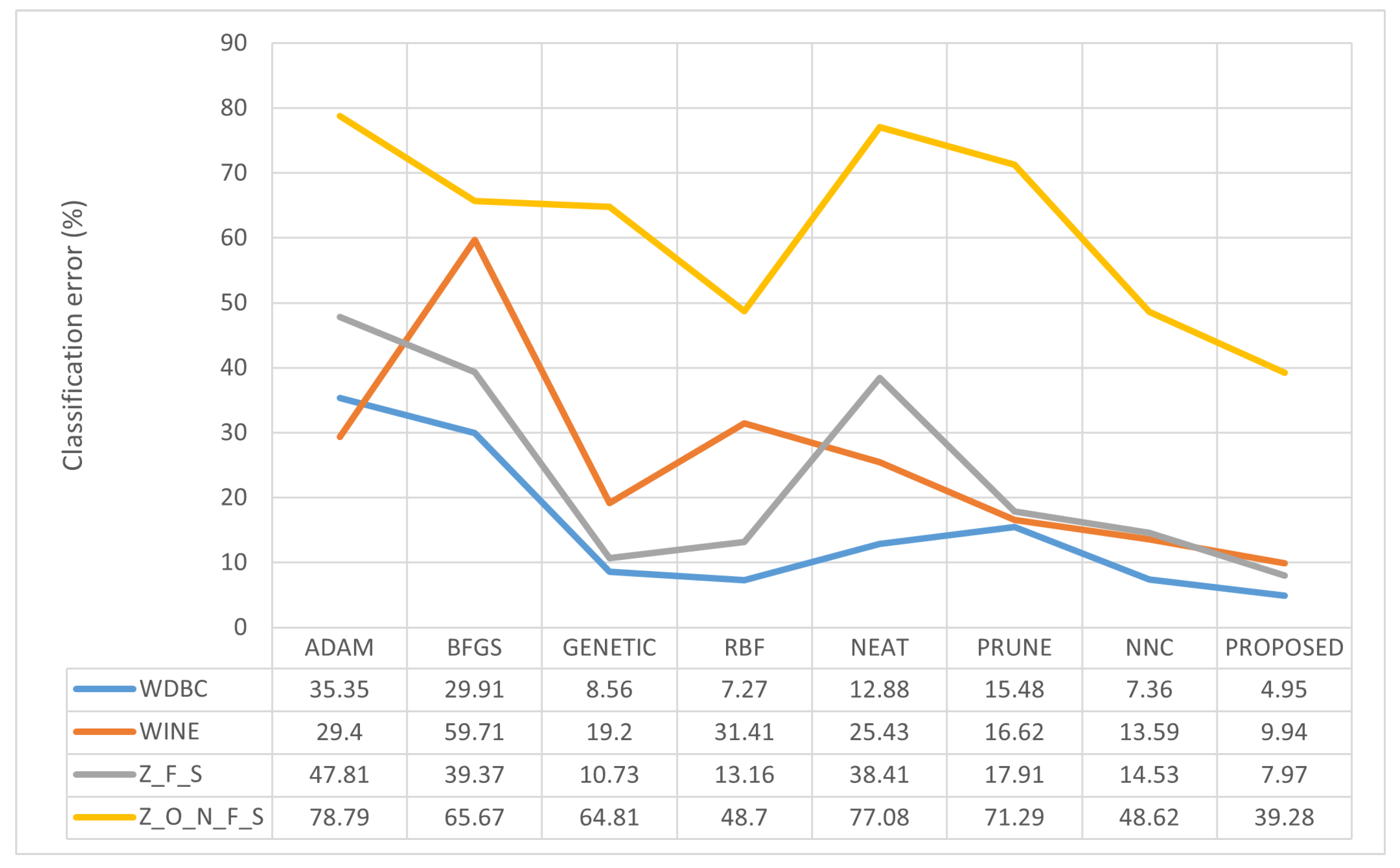
Based on Table 2 with 36 classification datasets and 9 methods (lower percentage implies lower error), the PROPOSED method attains the lowest mean error (21.18%) and the best average rank across datasets (1.83 on a 1–9 scale). The current work achieves the best result in 18 out of 36 datasets. The remaining per-dataset best results are distributed as follows: RBF 4, PRUNE 4, DNN 3, NEAT 3, NNC 3, and GENETIC 1, while ADAM and BFGS record no first-place finishes. In head-to-head, dataset-wise comparisons, the proposed method outperforms each alternative on the vast majority of datasets: vs ADAM on 35/36 datasets, vs. BFGS on 33/36, vs. GENETIC on 32/36, vs. RBF on 30/36, vs. NEAT on 33/36, vs. PRUNE on 31/36, vs. DNN on 32/36, and vs. NNC on 32/36. The average absolute error reduction of PROPOSED relative to each competitor, computed as “competitor — PROPOSED” in percentage points and then averaged over the 36 datasets, is 14.39 (ADAM), 13.51 (BFGS), 6.12 (GENETIC), 8.60 (RBF), 11.90 (NEAT), 7.53 (PRUNE), 6.64 (DNN), and 2.60 (NNC). The corresponding mean relative reductions, computed as (competitor — PROPOSED)/competitor and then averaged per dataset, are 39.24%, 34.29%, 22.83%, 26.50%, 37.09%, 20.91%, 22.95%, and 12.65%. The few datasets where the proposed method is worse are concentrated in specific cases: ADAM only on POPFAILURES; BFGS on CIRCULAR, PHONEME, and POPFAILURES; GENETIC on CIRCULAR, GLASS, LIVERDISORDER, and PHONEME; RBF on APPENDICITIS, CIRCULAR, GLASS, HABERMAN, LIVERDISORDER, and SPIRAL; NEAT on ECOLI, HABERMAN, and LIVERDISORDER; PRUNE on ALCOHOL, DERMATOLOGY, IONOSPHERE, LYMOGRAPHY, and POPFAILURES; DNN on HABERMAN, HOUSEVOTES, SEGMENT, and ZONF_S; and NNC on AUSTRALIAN, HEARTATTACK, HOUSEVOTES, and IONOSPHERE. The table’s AVERAGE row is consistent with this picture: PROPOSED has the lowest mean error (21.18%) among all methods. Relative to the second-best mean in that row (NNC: 24.79%), PROPOSED reduces error by 3.61 percentage points, corresponding to about a 14.56% relative reduction. Median errors tell the same story: PROPOSED has a median of 19.24%, lower than NNC (21.21%) and DNN (25.83%). Overall, PROPOSED shows consistent superiority in terms of error, as reflected by the mean, the across-dataset ranking, and the dataset-wise head-to-head counts, with only a small number of dataset-specific exceptions.
The average classification error for all methods is illustrated in Figure 7. Additionally, the dimension for each classification dataset and the number of distinct classes are provided in Table 3.
A line plot is provided in Figure 8 for a series of selected datasets to depict the effectiveness of the proposed method.
In Table 4, with 21 regression datasets and 9 methods (lower values indicate lower error), the proposed method achieves the lowest mean error (4.28 vs. 6.29 for NNC in the AVERAGE row) and the lowest median (0.036). Its average rank across datasets is 1.67 on a 1–9 scale, lower than any competitor (next best: NNC 3.83, DNN 4.69, RBF 4.79). At the dataset level, the current work is the strict winner on 12 of 21 datasets and ties for best on 2 more (AIRFOIL with PRUNE and LW with NNC), thus topping 14/21 datasets overall. The remaining first places are taken by ADAM (ABALONE and FY), GENETIC (FRIEDMAN and STOCK), RBF (BK and DEE), and NNC (HO). The gap from the dataset-wise best alternative is typically small: PROPOSED is within 5% of the best on 15/21 datasets and within 10% on 16/21, with the largest shortfalls appearing mainly on FRIEDMAN (5.34 vs. 1.249) and, more mildly, on DEE (0.22 vs. 0.17) and STOCK (4.69 vs. 3.88). In head-to-head, dataset-wise comparisons, PROPOSED has lower error than each alternative in the vast majority of cases: vs. ADAM it is better on 19/21 datasets (worse on ABALONE and FY), vs. BFGS on 20/21 (worse only on FRIEDMAN), vs. GENETIC on 19/21 (worse on FRIEDMAN and STOCK), vs. RBF on 18/21 (worse on BK, DEE, and FY), vs. NEAT on 21/21, vs. PRUNE on 19/21 with 1 tie (worse on FY), vs. DNN on 18/21 (worse on BK, FRIEDMAN, and FY), and vs. NNC on 19/21 with 1 tie (worse on HO, tie on LW). The average absolute error reduction of PROPOSED relative to each competitor, computed as “competitor — PROPOSED” and then averaged over the 21 datasets, is approximately 18.18 (ADAM), 26.01 (BFGS), 5.03 (GENETIC), 5.74 (RBF), 10.37 (NEAT), 11.12 (PRUNE), 7.00 (DNN), and 2.01 (NNC); the corresponding mean relative reductions are about 62%, 64%, 44%, 53%, 80%, 50%, 44%, and 46%. The AVERAGE row is consistent with this picture: PROPOSED has the lowest mean error (4.28), outperforming the second-best NNC by 2.01 units (about a 32% relative reduction when computed from the reported means) and leaving larger margins against DNN, RBF, GENETIC, PRUNE, NEAT, ADAM, and BFGS. Overall, PROPOSED exhibits consistent superiority in terms of error as reflected by mean and median values, average rank, and the per-dataset win counts, with the most notable exceptions confined to a few datasets that appear to have distinct error scales.
The statistical comparison, depicted in Figure 9, indicates that all pairwise comparisons between the current method and the alternative models are highly statistically significant. Under the conventional star notation, **** denotes p < 0.0001, while the ***** flag for PROPOSED vs. RBF signals even stronger statistical evidence in favor of PROPOSED. Overall, the findings confirm that PROPOSED consistently achieves lower error than every comparator across the classification datasets, with a negligible likelihood that these differences are due to chance.
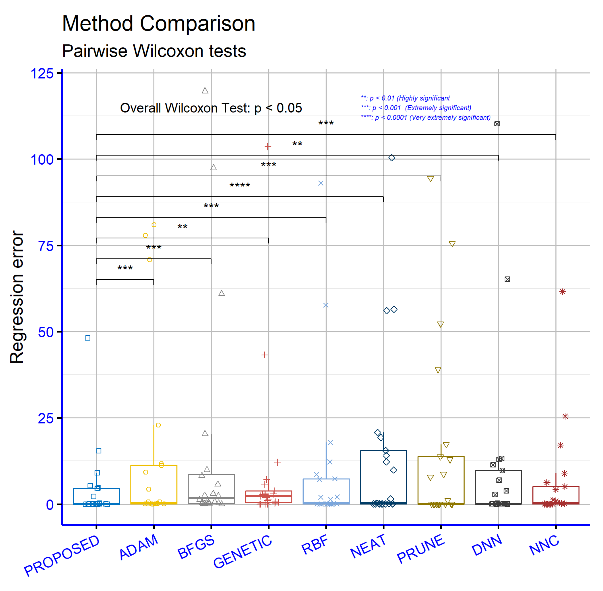
In Figure 10, the statistical comparison on the regression datasets indicates that the proposed model differs significantly from all alternative methods. Evidence is particularly strong against ADAM, BFGS, RBF, PRUNE, and NNC (p = ***, i.e., p ≤ 0.001), with the strongest signal observed against NEAT (p = ****, i.e., p ≤ 0.0001). Comparisons against GENETIC and DNN are also statistically significant but comparatively weaker (p = **, i.e., p ≤ 0.01). Taken together, the results consistently support that the proposed model attains lower error than every competing approach across the examined datasets, with a very low probability that the observed differences are due to chance. Note that significance levels reflect the strength of statistical evidence rather than effect magnitude; for a fuller interpretation it is advisable to also report absolute or relative error differences and suitable effect size metrics.

3.3. Experiments with a Different Crossover Mechanism

In order to illustrated the robustness of the proposed method, another experiment was conducted in which the uniform crossover procedure was used for the neural network construction method and the proposed one instead of the one-point crossover. The experimental results for the classification and regression datasets are shown, respectively, in Table 5 and Table 6. However, the one-point crossover mechanism is proposed as the crossover procedure in the original article of grammatical evolution.
Analysis of the results in Table 5 demonstrates that the proposed method systematically outperforms both variants of NNC, regardless of the crossover type employed. Specifically, the proposed method with one-point crossover achieves a significantly lower average error rate (21.18%) compared to NNC (24.79%). A similar performance gap is observed with uniform crossover, where the proposed method maintains superiority (22.32% vs. NNC’s 24.76%). The advantage is particularly pronounced in several datasets: for BALANCE (7.61–7.84% vs. 20.73–23.65%), CIRCULAR (6.92–11.86% vs. 12.66–17.59%), Z_F_S (7.97–10.13% vs. 14.53–18.33%), and ZO_NF_S (6.94–8.24% vs. 13.54–14.52%). Notably, in datasets like WDBC and WINE, the proposed method reduces the error by nearly half compared to NNC. Interestingly, the choice of crossover type shows minimal impact on performance for both methods. The marginal differences between one-point and uniform crossover (with average errors remaining stable for each method) suggest that the proposed method’s superiority stems from its fundamental architecture rather than the recombination technique. These experimental results confirm the robustness of the proposed method, which maintains consistent superiority across various classification datasets while significantly reducing average error rates compared to standard NNC approaches.
Table 6 further validates the proposed method’s superiority for regression datasets. The proposed method achieves lower average errors with both one-point (4.28) and uniform crossover (4.74) compared to NNC (6.29 and 6.66, respectively). The performance gap is especially notable in key datasets: AUTO (9.09–11.1 vs. 17.13–20.06), HOUSING (15.47–16.89 vs. 25.47–26.68), and PLASTIC (2.17–2.3 vs. 4.2–5.2). In several cases (AIRFOIL, LASER, MORTGAGE), the proposed method reduces errors to a fraction of NNC’s values. Particularly impressive results appear in BL (0.001) and QUAKE (0.036), where the proposed method achieves remarkably low, crossover-invariant errors. The crossover type shows slightly less impact on the proposed method (average difference of 0.46) than on NNC (0.37 difference), though one-point crossover yields marginally better results for both. These comprehensive results confirm that the proposed method maintains its superiority in regression problems, delivering consistently and significantly improved performance over NNC. Its ability to achieve lower errors across diverse problems, independent of crossover selection, solidifies its position as a more reliable and effective approach.

3.4. Experiments with the Critical Parameter N K

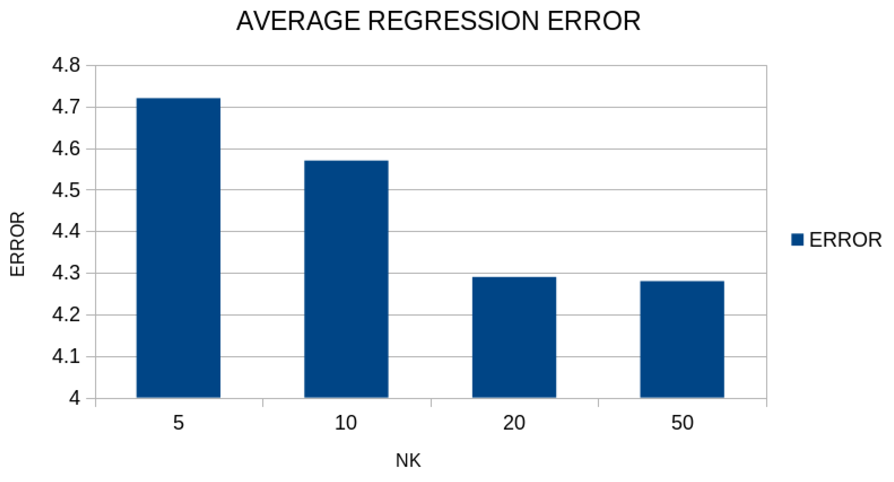
Another experiment was conducted where the parameter N K was altered in the range [ 5 , , 50 ] , and the results for the regression datasets are depicted in Figure 11.
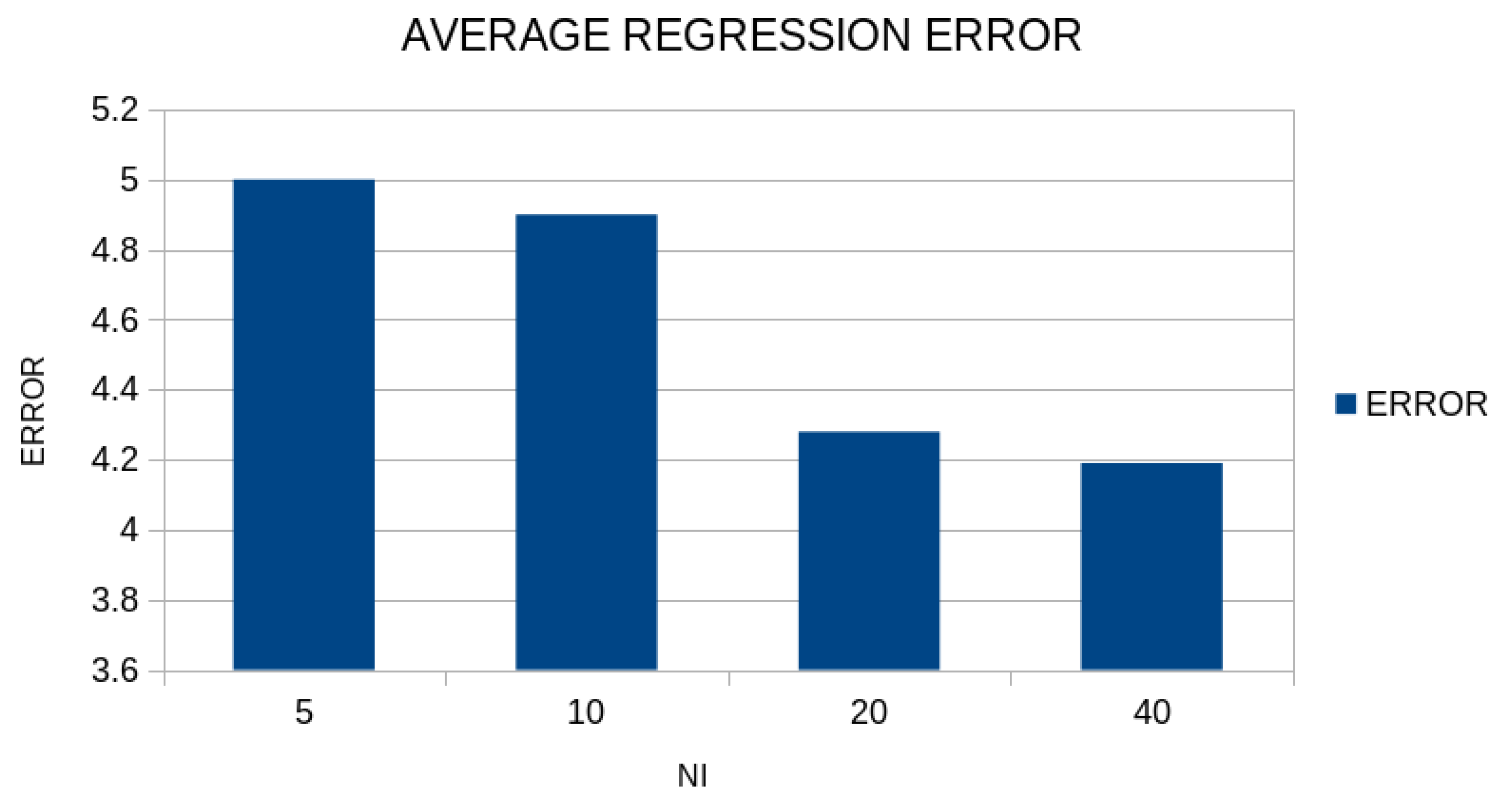
Additionally, a series of experiments was conducted where the parameter N I was changed from 10 to 40, and the results are graphically presented in Figure 12.
This figure presents the relationship between the number of chromosomes ( N I ) participating in the secondary genetic algorithm and the resulting regression error. We observe that as the number of chromosomes increases, the error decreases, indicating improvement in the model’s performance. Specifically, for N I = 5 , the error is 4.99, while for N I = 10 , the error drops to 4.89. This trend continues with further increase in chromosomes: for N I = 20 , the error reaches 4.27, and for N I = 40 , the error reaches 4.18. This error reduction shows that using more chromosomes in the secondary genetic algorithm leads to better optimization of the neural network’s parameters, resulting in error minimization. However, the improvement is not linear. We observe that the difference in error between N I = 5 and N I = 10 is 0.10, while between N I = 20 and N I = 40 it is only 0.09. This may indicate that beyond a certain point, increasing chromosomes has progressively smaller impact on error reduction. This phenomenon may be due to factors such as algorithm convergence or the existence of an optimization threshold beyond which improvement becomes more difficult. Furthermore, the selection of N I may be influenced by computational constraints. Using more chromosomes increases the computational load, so the performance improvement must be balanced against resource costs. For example, transitioning from N I = 20 to N I = 40 leads to error reduction of only 0.09, which may not justify the doubling of computational cost in certain scenarios. In summary, the table confirms that increasing the number of chromosomes improves the model’s performance, but its effect becomes smaller as N I grows larger. This means that the optimal selection of N I depends on a combination of factors, such as the desired accuracy, available computational resources, and the nature of the problem.
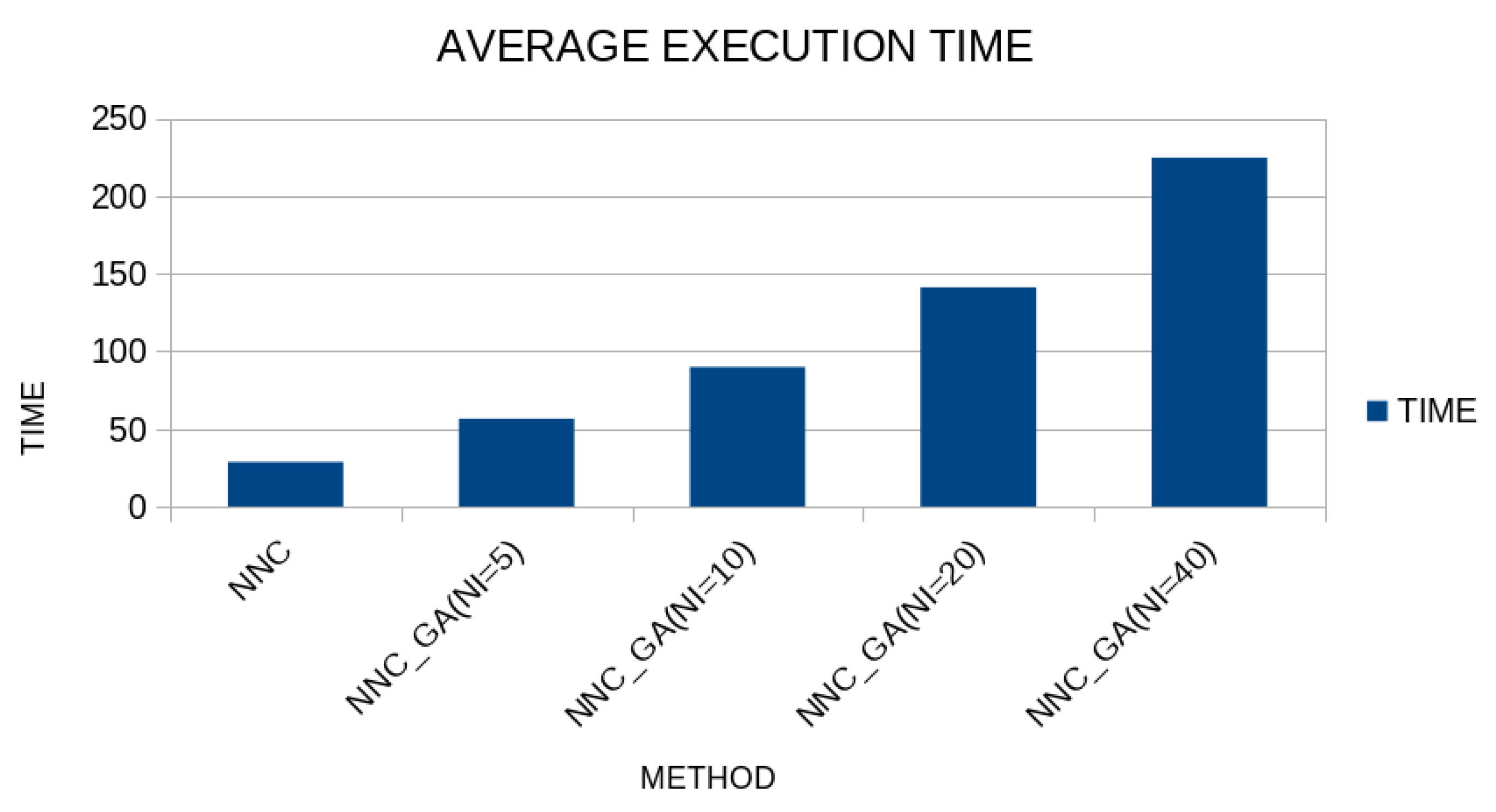
In Figure 13, the average execution time for the regression dataset is plotted. In this graph the original neural network construction method is depicted as well as the proposed one using a series of values for the parameter N I . As was expected, the execution time increases when the parameter N I is increased.

3.5. A Series of Practical Examples

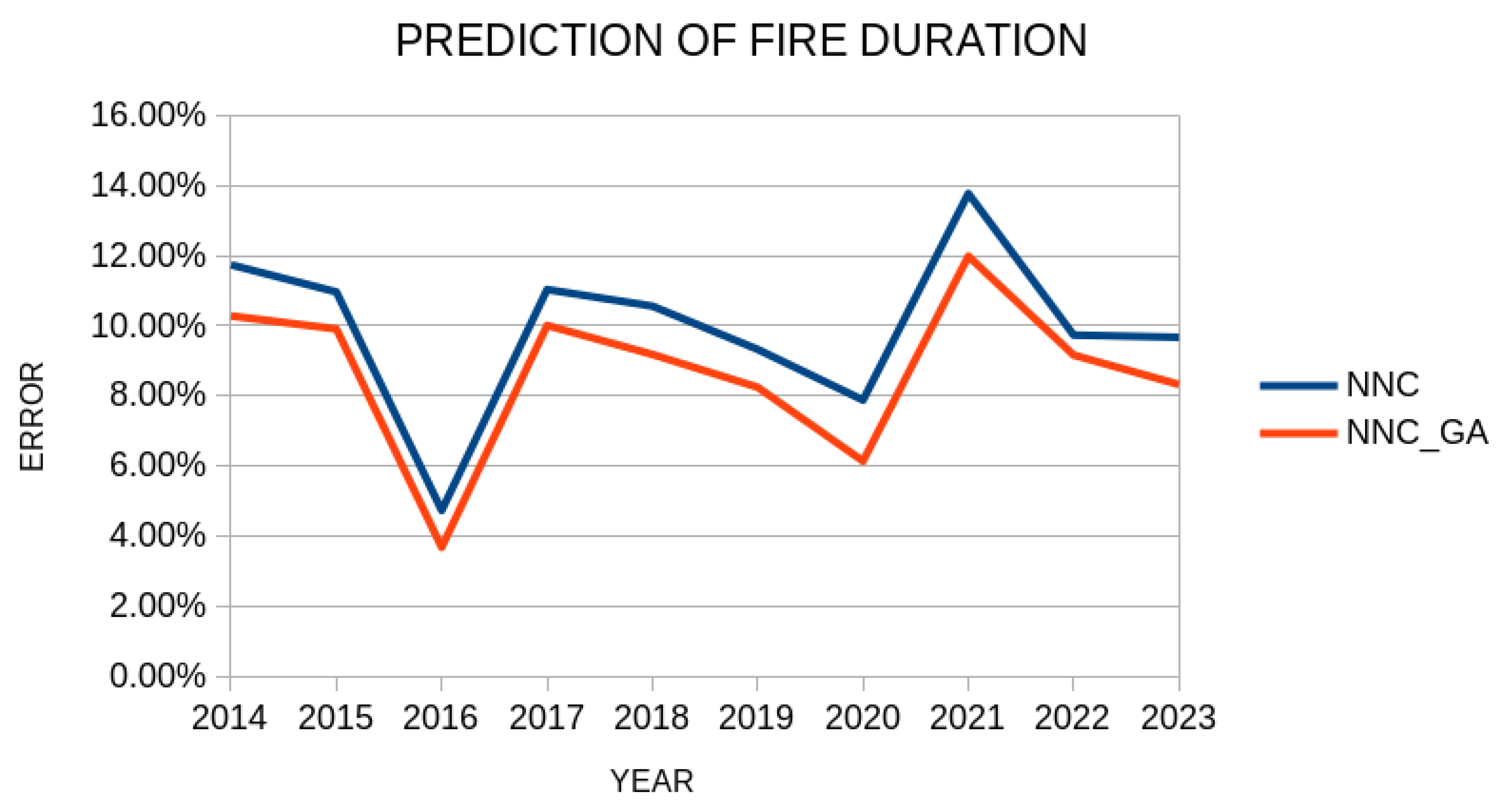
As practical applications of the proposed method to real-world problems, we consider two cases from the recent bibliography. In the first case, consider the prediction of the duration of forest fires as presented for the Greek territory in a recent publication [113]. Using data from the Greek Fire Service, an attempt is made to predict the duration of forest fires for the years 2014–2023. Figure 14 depicts a comparison for the classification error for this problem for the years 2014–2023 between the original neural network construction method, denoted as NNC, and the proposed method, which is denoted as NNC_GA in the plot.
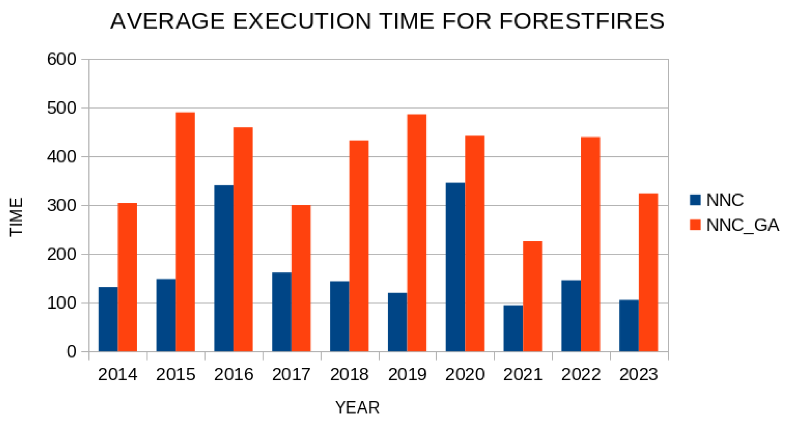
As is evident, the proposed method has a lower error in estimating the duration of forest fires in all years from 2014 to 2023 compared to the original artificial neural network construction technique. However, the proposed method requires significantly more time than the original method, as depicted in Figure 15.
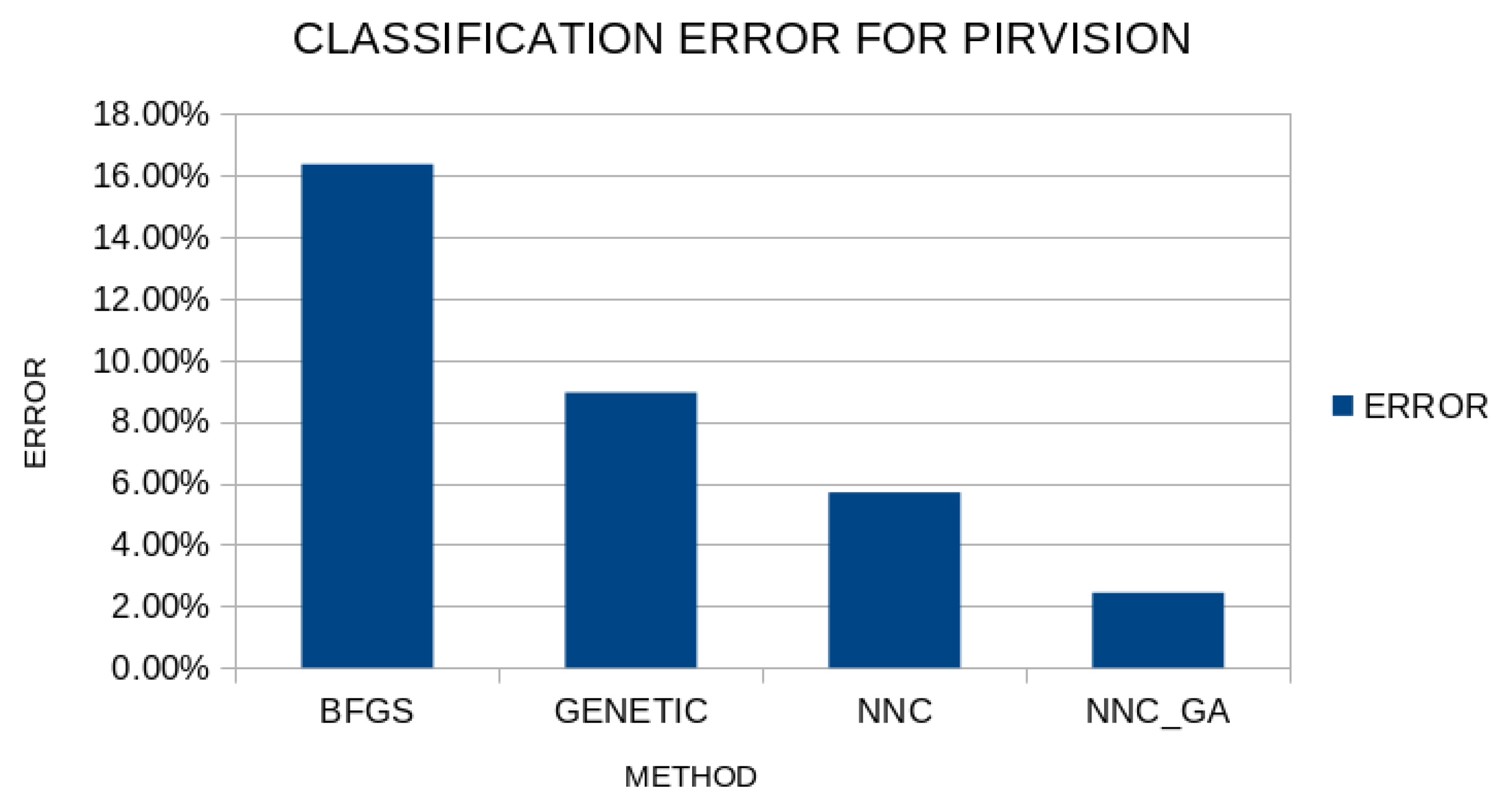
The second practical example is the PIRvision dataset [114], which contains occupancy detection data that was collected from a synchronized low-energy electronically chopped passive infrared sensing node in residential and office environments. The dataset contains 15,302 patterns, and the dimension of each pattern is 59. The experimental results, validated with ten-fold cross validation using a series of methods and the proposed one, are depicted in Figure 16.
It is evident that the proposed modification of the neural network construction method significantly outperforms the other techniques in terms of average classification error for this particular dataset.

4. Discussion

This study presents an interesting approach combining grammatical evolution with modified genetic algorithms for constructing artificial neural networks. However, a comprehensive analysis of the results and practical implications reveals several aspects that require further investigation and critical examination. While the experimental findings demonstrate certain improvements over traditional techniques, the interpretation and significance of these improvements have not been analyzed with the depth and critical thinking required for a complete method evaluation. Regarding classification performance, the method shows an average error rate of 21.18% compared to ADAM’s 36.45% and BFGS’s 35.71%. However, these comparative metrics conceal significant performance variations across different datasets. For instance, on Cleveland and Ecoli datasets, classification error reaches 46.41% and 48.82%, respectively, while on Housevotes and Zoo, it drops below 7%. This substantial performance variation suggests the method may be highly sensitive to dataset-specific characteristics, which is not sufficiently analyzed in the results presentation. Furthermore, the lack of analysis regarding variation across the 30 repetitions of each experiment raises questions about the method’s stability and reliability in real-world applications. The statistical significance of results, while supported by extremely low p-values (1.9 × 10⁻⁷ to 1.1 × 10⁻⁸), does not account for the dynamics of different problem types. In noisy datasets or those with significant class imbalance like Haberman and Liverdisorder, the method shows notable performance fluctuations that remain unexplained. Additionally, the absence of analysis regarding dataset characteristics affecting performance (such as dimensionality, sample size, or degree of linear separability) makes it difficult to determine the optimal conditions for the method’s application. Computational resources and execution times present another critical but underexplored issue.
While the study mentions using an AMD Ryzen 5950X system with 128 GB RAM, comprehensive reporting of computational requirements is missing. Specifically, it would be essential to present average training times per dataset category (classification vs. regression), the method’s scalability regarding number of features and samples, memory consumption during the grammatical evolution process, and the impact of various parameters (like population size and generation count) on execution times. This lack of information makes practical implementation assessment challenging, especially for real-world problems where computational resources and time constraints are crucial factors. Regarding limitations, while the study acknowledges issues like local optima and overfitting, their analysis remains superficial. For example, in datasets like Z_O_N_F_S with 39.28% error, it is not investigated whether this results from insufficient solution space exploration due to grammatical evolution parameters, limitations in the grammar used for architecture generation, excessive network complexity leading to overfitting, or inadequacies in parameter training mechanisms. Practical application and robustness require more thorough examination. Beyond controlled experimental scenarios, there is missing information about the ease of applying the method to real-world, unprocessed datasets, the required expertise for optimal parameter tuning, the method’s resilience to noisy, incomplete, or imbalanced data, and the interpretability of results and generated architectures. Moreover, comparisons with contemporary approaches like transformers, convolutional neural networks, or reinforcement learning methods in domains where they dominate (e.g., natural language processing, computer vision, robotics) are completely absent from the study. This evaluation gap significantly limits our understanding of the method’s relative value compared to state-of-the-art alternatives. The method’s generalizability to new application domains has not been adequately explored. While results are presented across various fields (medicine, physics, economics), critical information is missing about the flexibility and adaptability of the used grammar across different domains, required modifications for new data types (time series, graphs, spatial data), knowledge transfer capability between different applications, and domain knowledge requirements for appropriate grammar design. In summary, while the proposed method introduces interesting mechanisms for improving automated neural network design, this analysis reveals numerous aspects needing further investigation.
For a complete and objective evaluation, it would be necessary to conduct a much more detailed analysis of result stability and variation, comparisons with alternative contemporary approaches beyond the basic techniques examined, thorough evaluation of scalability and computational requirements for large datasets, in-depth investigation of real-world implementation challenges and limitations, and analysis of generalization and adaptation capability to new domains and data types. Only through such a holistic and critical approach could we obtain a complete picture of this methodology’s value, capabilities, and limitations. The current results, while encouraging, leave significant gaps in our understanding of how and under what conditions the method can truly provide value compared to existing approaches in automated neural network design.

5. Conclusions

The article presents a method for constructing artificial neural networks by integrating grammatical evolution (GE) with a modified genetic algorithm (GA) to improve generalization properties and reduce overfitting. The method proves to be effective in designing neural network architectures and optimizing their parameters. The modified genetic algorithm avoids local minima during training and addresses overfitting by applying penalty factors to the fitness function, ensuring better generalization to unseen data. The method was evaluated on a variety of classification and regression datasets from diverse fields, including physics, chemistry, medicine, and economics. Comparative results indicate that the proposed method achieves lower error rates on average compared to traditional optimization and machine learning techniques, highlighting its stability and adaptability. The results, analyzed through statistical metrics such as p-values, provide strong evidence of the method’s superiority over competing models in both classification and regression tasks. A key innovation of the method is the combination of dynamic architecture generation and parameter optimization within a unified framework. This approach not only enhances performance but also reduces the computational complexity associated with manually designing neural networks. Additionally, the use of constraint techniques in the genetic algorithm ensures the preservation of the neural network structure while enabling controlled optimization of parameters. Future explorations could focus on testing the method on larger and more complex datasets, such as those encountered in image recognition, natural language processing, and genomics, to evaluate its scalability and effectiveness in real-world applications. Furthermore, the integration of other global optimization methods, such as particle swarm optimization, simulated annealing, or differential evolution, could be considered to further enhance the algorithm’s robustness and convergence speed. Concurrently, the inclusion of regularization techniques, such as dropout or batch normalization, could improve the method’s generalization capabilities even further. Reducing computational cost is another important area of investigation, and the method could be adapted to leverage parallel computing architectures, such as GPUs or distributed systems, making it feasible for training on large datasets or for real-time applications. Finally, customizing the grammar used in grammatical evolution based on the specific characteristics of individual fields could improve the method’s performance in specialized tasks, such as time-series forecasting or anomaly detection in cybersecurity.
The proposed technique attempts to maintain the parameters of artificial neural networks within ranges of values in which the neural network is likely to have good generalization properties. A possible future improvement could be to find this interval of values either with some technique that utilizes derivatives or with interval arithmetic techniques [115,116].

Author Contributions

V.C. and I.G.T. conducted the experiments employing several datasets and provided the comparative experiments. D.T. and V.C. performed the statistical analysis and prepared the manuscript. All authors have read and agreed to the published version of the manuscript.

Funding

This research has been financed by the European Union: Next Generation EU through the Program Greece 2.0 National Recovery and Resilience Plan, under the call RESEARCH–CREATE–INNOVATE, project name “iCREW: Intelligent small craft simulator for advanced crew training using Virtual Reality techniques” (project code: TAEDK-06195).

Data Availability Statement

The original contributions presented in this study are included in the article. Further inquiries can be directed to the corresponding author.

Conflicts of Interest

The authors declare no conflicts of interest.

References

  1. Abiodun, O.I.; Jantan, A.; Omolara, A.E.; Dada, K.V.; Mohamed, N.A.; Arshad, H. State-of-the-art in artificial neural network applications: A survey. Heliyon 2018, 4, e00938. [Google Scholar] [CrossRef] [PubMed]
  2. Suryadevara, S.; Yanamala, A.K.Y. A Comprehensive Overview of Artificial Neural Networks: Evolution, Architectures, and Applications. Rev. Intel. Artif. Med. 2021, 12, 51–76. [Google Scholar]
  3. Egmont-Petersen, M.; de Ridder, D.; Handels, H. Image processing with neural networks—A review. Pattern Recognit. 2002, 35, 2279–2301. [Google Scholar] [CrossRef]
  4. Zhang, G.P. Time series forecasting using a hybrid ARIMA and neural network model. Neurocomputing 2003, 50, 159–175. [Google Scholar] [CrossRef]
  5. Huang, Z.; Chen, H.; Hsu, C.-J.; Chen, W.-H.; Wu, S. Credit rating analysis with support vector machines and neural networks: A market comparative study. Decis. Support Syst. 2004, 37, 543–558. [Google Scholar] [CrossRef]
  6. Baldi, P.; Cranmer, K.; Faucett, T.; Sadowski, P.; Whiteson, D. Parameterized neural networks for high-energy physics. Eur. Phys. J. C 2016, 76, 1–7. [Google Scholar] [CrossRef]
  7. Aguirre, L.A.; Lopes, R.A.; Amaral, G.F.; Letellier, C. Constraining the topology of neural networks to ensure dynamics with symmetry properties. Phys. Rev. E 2004, 69, 026701. [Google Scholar] [CrossRef] [PubMed]
  8. Mattheakis, M.; Protopapas, P.; Sondak, D.; Di Giovanni, M.; Kaxiras, E. Physical symmetries embedded in neural networks. arXiv 2019, arXiv:1904.08991. [Google Scholar]
  9. Krippendorf, S.; Syvaeri, M. Detecting symmetries with neural networks. Mach. Learn. Sci. Technol. 2020, 2, 015010. [Google Scholar] [CrossRef]
  10. Vora, K.; Yagnik, S. A survey on backpropagation algorithms for feedforward neural networks. Int. J. Eng. Dev. Res. 2014, 1, 193–197. [Google Scholar]
  11. Pajchrowski, T.; Zawirski, K.; Nowopolski, K. Neural speed controller trained online by means of modified RPROP algorithm. IEEE Trans. Ind. Inform. 2014, 11, 560–568. [Google Scholar] [CrossRef]
  12. Hermanto, R.P.S.; Nugroho, A. Waiting-time estimation in bank customer queues using RPROP neural networks. Procedia Comput. Sci. 2018, 135, 35–42. [Google Scholar] [CrossRef]
  13. Kingma, D.P.; Ba, J.L. ADAM: A method for stochastic optimization. In Proceedings of the 3rd International Conference on Learning Representations (ICLR 2015), San Diego, CA, USA, 7–9 May 2015; pp. 1–15. [Google Scholar]
  14. Reynolds, J.; Rezgui, Y.; Kwan, A.; Piriou, S. A zone-level, building energy optimisation combining an artificial neural network, a genetic algorithm, and model predictive control. Energy 2018, 151, 729–739. [Google Scholar] [CrossRef]
  15. Das, G.; Pattnaik, P.K.; Padhy, S.K. Artificial neural network trained by particle swarm optimization for non-linear channel equalization. Expert Syst. Appl. 2014, 41, 3491–3496. [Google Scholar] [CrossRef]
  16. Sexton, R.S.; Dorsey, R.E.; Johnson, J.D. Beyond backpropagation: Using simulated annealing for training neural networks. J. Organ. End User Comput. (JOEUC) 1999, 11, 3–10. [Google Scholar] [CrossRef]
  17. Wang, L.; Zeng, Y.; Chen, T. Back propagation neural network with adaptive differential evolution algorithm for time series forecasting. Expert Syst. Appl. 2015, 42, 855–863. [Google Scholar] [CrossRef]
  18. Karaboga, D.; Akay, B. Artificial bee colony (ABC) algorithm on training artificial neural networks. In Proceedings of the 2007 IEEE 15th Signal Processing and Communications Applications, Eskisehir, Turkey, 11–13 June 2007; IEEE: New York, NY, USA, 2007; pp. 1–4. [Google Scholar]
  19. Sexton, R.S.; Alidaee, B.; Dorsey, R.E.; Johnson, J.D. Global optimization for artificial neural networks: A tabu search application. Eur. J. Oper. Res. 1998, 106, 570–584. [Google Scholar] [CrossRef]
  20. Zhang, J.-R.; Zhang, J.; Lok, T.-M.; Lyu, M.R. A hybrid particle swarm optimization–back-propagation algorithm for feedforward neural network training. Appl. Math. Comput. 2007, 185, 1026–1037. [Google Scholar] [CrossRef]
  21. Zhao, G.; Wang, T.; Jin, Y.; Lang, C.; Li, Y.; Ling, H. The Cascaded Forward algorithm for neural network training. Pattern Recognit. 2025, 161, 111292. [Google Scholar] [CrossRef]
  22. Oh, K.; Jung, K. GPU implementation of neural networks. Pattern Recognit. 2004, 37, 1311–1314. [Google Scholar] [CrossRef]
  23. Zhang, M.; Hibi, K.; Inoue, J. GPU-accelerated artificial neural network potential for molecular dynamics simulation. Comput. Commun. 2023, 285, 108655. [Google Scholar] [CrossRef]
  24. Nowlan, S.J.; Hinton, G.E. Simplifying neural networks by soft weight sharing. Neural Comput. 1992, 4, 473–493. [Google Scholar] [CrossRef]
  25. Nowlan, S.J.; Hinton, G.E. Simplifying neural networks by soft weight sharing. In The Mathematics of Generalization; CRC Press: Boca Raton, FL, USA, 2018; pp. 373–394. [Google Scholar]
  26. Hanson, S.J.; Pratt, L.Y. Comparing biases for minimal network construction with back propagation. In Advances in Neural Information Processing Systems; Touretzky, D.S., Ed.; Morgan Kaufmann: San Mateo, CA, USA, 1989; Volume 1, pp. 177–185. [Google Scholar]
  27. Augasta, M.; Kathirvalavakumar, T. Pruning algorithms of neural networks—A comparative study. Cent. Eur. Comput. Sci. 2003, 3, 105–115. [Google Scholar] [CrossRef]
  28. Prechelt, L. Automatic early stopping using cross validation: Quantifying the criteria. Neural Netw. 1998, 11, 761–767. [Google Scholar] [CrossRef]
  29. Wu, X.; Liu, J. A New Early Stopping Algorithm for Improving Neural Network Generalization. In Proceedings of the 2009 Second International Conference on Intelligent Computation Technology and Automation, Changsha, Hunan, 10–11 October 2009; pp. 15–18. [Google Scholar]
  30. Treadgold, N.K.; Gedeon, T.D. Simulated annealing and weight decay in adaptive learning: The SARPROP algorithm. IEEE Trans. Neural Netw. 1998, 9, 662–668. [Google Scholar] [CrossRef]
  31. Carvalho, M.; Ludermir, T.B. Particle Swarm Optimization of Feed-Forward Neural Networks with Weight Decay. In Proceedings of the 2006 Sixth International Conference on Hybrid Intelligent Systems (HIS’06), Auckland, New Zealand, 13–15 December 2006; pp. 13–15. [Google Scholar]
  32. Arifovic, J.; Gençay, R. Using genetic algorithms to select architecture of a feedforward artificial neural network. Phys. A Stat. Mech. Appl. 2001, 289, 574–594. [Google Scholar] [CrossRef]
  33. Benardos, P.G.; Vosniakos, G.C. Optimizing feedforward artificial neural network architecture. Eng. Appl. Artif. Intell. 2007, 20, 365–382. [Google Scholar] [CrossRef]
  34. Garro, B.A.; Vázquez, R.A. Designing Artificial Neural Networks Using Particle Swarm Optimization Algorithms. Comput. Neurosci. 2015, 2015, 369298. [Google Scholar] [CrossRef]
  35. Siebel, N.T.; Sommer, G. Evolutionary reinforcement learning of artificial neural networks. Int. Hybrid Intell. Syst. 2007, 4, 171–183. [Google Scholar] [CrossRef]
  36. Jaafra, Y.; Laurent, J.L.; Deruyver, A.; Naceur, M.S. Reinforcement learning for neural architecture search: A review. Image Vis. Comput. 2019, 89, 57–66. [Google Scholar] [CrossRef]
  37. Pham, H.; Guan, M.; Zoph, B.; Le, Q.; Dean, J. Efficient neural architecture search via parameters sharing. In Proceedings of the International Conference on Machine Learning, Stockholm, Sweden, 10–15 July 2018; pp. 4095–4104. [Google Scholar]
  38. Xie, S.; Zheng, H.; Liu, C.; Lin, L. SNAS: Stochastic neural architecture search. arXiv 2018, arXiv:1812.09926. [Google Scholar]
  39. Zhou, H.; Yang, M.; Wang, J.; Pan, W. Bayesnas: A bayesian approach for neural architecture search. In Proceedings of the International Conference on Machine Learning, Long Beach, CA, USA, 10–15 June 2019; pp. 7603–7613. [Google Scholar]
  40. Terfloth, L.; Gasteige, J. Neural networks and genetic algorithms in drug design. Drug Discov. Today 2001, 6, 102–108. [Google Scholar] [CrossRef]
  41. Kim, G.H.; Seo, D.S.; Kang, K.I. Hybrid models of neural networks and genetic algorithms for predicting preliminary cost estimates. J. Comput. In Civil Eng. 2005, 19, 208–211. [Google Scholar] [CrossRef]
  42. Kalogirou, S.A. Optimization of solar systems using artificial neural-networks and genetic algorithms. Appl. Energy 2004, 77, 383–405. [Google Scholar] [CrossRef]
  43. Tong, D.L.; Mintram, R. Genetic Algorithm-Neural Network (GANN): A study of neural network activation functions and depth of genetic algorithm search applied to feature selection. Int. J. Mach. Learn. Cyber. 2010, 1, 75–87. [Google Scholar] [CrossRef]
  44. Ruehle, F. Evolving neural networks with genetic algorithms to study the string landscape. J. High Energ. Phys. 2017, 2017, 38. [Google Scholar] [CrossRef]
  45. Ghosh, S.C.; Sinha, B.P.; Das, N. Channel assignment using genetic algorithm based on geometric symmetry. IEEE Trans. Veh. Technol. 2003, 52, 860–875. [Google Scholar] [CrossRef]
  46. Liu, Y.; Zhou, D. An Improved Genetic Algorithm with Initial Population Strategy for Symmetric TSP. Math. Probl. Eng. 2015, 2015, 212794. [Google Scholar] [CrossRef]
  47. Han, S.; Barcaro, G.; Fortunelli, A.; Lysgaard, S.; Vegge, T.; Hansen, H.A. Unfolding the structural stability of nanoalloys via symmetry-constrained genetic algorithm and neural network potential. NPJ Comput. Mater. 2022, 8, 121. [Google Scholar] [CrossRef]
  48. O’Neill, M.; Ryan, C. Grammatical evolution. IEEE Trans. Evol. Comput. 2001, 5, 349–358. [Google Scholar] [CrossRef]
  49. Tsoulos, I.G.; Gavrilis, D.; Glavas, E. Neural network construction and training using grammatical evolution. Neurocomputing 2008, 72, 269–277. [Google Scholar] [CrossRef]
  50. Papamokos, G.V.; Tsoulos, I.G.; Demetropoulos, I.N.; Glavas, E. Location of amide I mode of vibration in computed data utilizing constructed neural networks. Expert Syst. Appl. 2009, 36, 12210–12213. [Google Scholar] [CrossRef]
  51. Tsoulos, I.G.; Gavrilis, D.; Glavas, E. Solving differential equations with constructed neural networks. Neurocomputing 2009, 72, 2385–2391. [Google Scholar] [CrossRef]
  52. Tsoulos, I.G.; Mitsi, G.; Stavrakoudis, A.; Papapetropoulos, S. Application of Machine Learning in a Parkinson’s Disease Digital Biomarker Dataset Using Neural Network Construction (NNC) Methodology Discriminates Patient Motor Status. Front. ICT 2019, 6, 10. [Google Scholar] [CrossRef]
  53. Christou, V.; Tsoulos, I.G.; Loupas, V.; Tzallas, A.T.; Gogos, C.; Karvelis, P.S.; Antoniadis, N.; Glavas, E.; Giannakeas, N. Performance and early drop prediction for higher education students using machine learning. Expert Syst. Appl. 2023, 225, 120079. [Google Scholar] [CrossRef]
  54. Toki, E.I.; Pange, J.; Tatsis, G.; Plachouras, K.; Tsoulos, I.G. Utilizing Constructed Neural Networks for Autism Screening. Appl. Sci. 2024, 14, 3053. [Google Scholar] [CrossRef]
  55. Backus, J.W. The Syntax and Semantics of the Proposed International Algebraic Language of the Zurich ACM-GAMM Conference. In Proceedings of the International Conference on Information Processing, UNESCO, Paris, France, 15–20 June 1959; pp. 125–132. [Google Scholar]
  56. Ryan, C.; Collins, J.; O’Neill, M. Grammatical evolution: Evolving programs for an arbitrary language. In Proceedings of the Genetic Programming EuroGP 1998, Paris, France, 14–15 April 1998; Lecture Notes in Computer Science. Banzhaf, W., Poli, R., Schoenauer, M., Fogarty, T.C., Eds.; Springer: Berlin/Heidelberg, Germany, 1998; Volume 1391. [Google Scholar]
  57. O’Neill, M.; Ryan, M.C. Evolving Multi-line Compilable C Programs. In Proceedings of the Genetic Programming EuroGP 1999, Goteborg, Sweden, 26–27 May 1999; Lecture Notes in Computer Science. Poli, R., Nordin, P., Langdon, W.B., Fogarty, T.C., Eds.; Springer: Berlin/Heidelberg, Germany, 1999; Volume 1598. [Google Scholar]
  58. Puente, A.O.; Alfonso, R.S.; Moreno, M.A. Automatic composition of music by means of grammatical evolution. In Proceedings of the APL ’02: Proceedings of the 2002 Conference on APL: Array Processing Languages: Lore, Problems, and Applications, Madrid, Spain, 22–25 July 2002; pp. 148–155. [Google Scholar]
  59. Galván-López, E.; Swafford, J.M.; O’Neill, M.; Brabazon, A. Evolving a Ms. PacMan Controller Using Grammatical Evolution. In Applications of Evolutionary Computation. EvoApplications 2010; Lecture Notes in Computer Science; Springer: Berlin/Heidelberg, Germany, 2010; Volume 6024. [Google Scholar]
  60. Shaker, N.; Nicolau, M.; Yannakakis, G.N.; Togelius, J.; O’Neill, M. Evolving levels for Super Mario Bros using grammatical evolution. In Proceedings of the 2012 IEEE Conference on Computational Intelligence and Games (CIG), Granada, Spain, 11–14 September 2012; pp. 304–311. [Google Scholar]
  61. Martínez-Rodríguez, D.; Colmenar, J.M.; Hidalgo, J.I.; Micó, R.J.V.; Salcedo-Sanz, S. Particle swarm grammatical evolution for energy demand estimation. Energy Sci. Eng. 2020, 8, 1068–1079. [Google Scholar] [CrossRef]
  62. Ryan, C.; Kshirsagar, M.; Vaidya, G.; Cunningham, A.; Sivaraman, R. Design of a cryptographically secure pseudo random number generator with grammatical evolution. Sci. Rep. 2022, 12, 8602. [Google Scholar] [CrossRef]
  63. Martín, C.; Quintana, D.; Isasi, P. Grammatical Evolution-based ensembles for algorithmic trading. Appl. Soft Comput. 2019, 84, 105713. [Google Scholar] [CrossRef]
  64. Anastasopoulos, N.; Tsoulos, I.G.; Karvounis, E.; Tzallas, A. Locate the Bounding Box of Neural Networks with Intervals. Neural Process Lett. 2020, 52, 2241–2251. [Google Scholar] [CrossRef]
  65. Kelly, M.; Longjohn, R.; Nottingham, K. The UCI Machine Learning Repository. Available online: https://archive.ics.uci.edu (accessed on 10 September 2025).
  66. Alcalá-Fdez, J.; Fernandez, A.; Luengo, J.; Derrac, J.; García, S.; Sánchez, L.; Herrera, F. KEEL Data-Mining Software Tool: Data Set Repository, Integration of Algorithms and Experimental Analysis Framework. J. Mult.-Valued Log. Soft Comput. 2011, 17, 255–287. [Google Scholar]
  67. Weiss, S.M.; Kulikowski, C.A. Computer Systems That Learn: Classification and Prediction Methods from Statistics, Neural Nets. In Machine Learning, and Expert Systems; Morgan Kaufmann Publishers Inc.: Burlington, MA, USA, 1991. [Google Scholar]
  68. Tzimourta, K.D.; Tsoulos, I.; Bilero, I.T.; Tzallas, A.T.; Tsipouras, M.G.; Giannakeas, N. Direct Assessment of Alcohol Consumption in Mental State Using Brain Computer Interfaces and Grammatical Evolution. Inventions 2018, 3, 51. [Google Scholar] [CrossRef]
  69. Quinlan, J.R. Simplifying Decision Trees. Int. J. Man-Mach. Stud. 1987, 27, 221–234. [Google Scholar] [CrossRef]
  70. Shultz, T.; Mareschal, D.; Schmidt, W. Modeling Cognitive Development on Balance Scale Phenomena. Mach. Learn. 1994, 16, 59–88. [Google Scholar] [CrossRef]
  71. Zhou, Z.H.; Jiang, Y. NeC4.5: Neural ensemble based C4.5. IEEE Trans. Knowl. Data Engineering 2004, 16, 770–773. [Google Scholar] [CrossRef]
  72. Setiono, R.; Leow, W.K. FERNN: An Algorithm for Fast Extraction of Rules from Neural Networks. Appl. Intell. 2000, 12, 15–25. [Google Scholar] [CrossRef]
  73. Demiroz, G.; Govenir, H.A.; Ilter, N. Learning Differential Diagnosis of Eryhemato-Squamous Diseases using Voting Feature Intervals. Artif. Intell. Med. 1998, 13, 147–165. [Google Scholar]
  74. Horton, P.; Nakai, K. A Probabilistic Classification System for Predicting the Cellular Localization Sites of Proteins. In Proceedings of the International Conference on Intelligent Systems for Molecular Biology, St. Louis, MO, USA, 12–15 June 1996; Volume 4, pp. 109–115. [Google Scholar]
  75. Hayes-Roth, B.; Hayes-Roth, B.F. Concept learning and the recognition and classification of exemplars. J. Verbal Learn. Verbal Behav. 1977, 16, 321–338. [Google Scholar] [CrossRef]
  76. Kononenko, I.; Šimec, E.; Robnik-Šikonja, M. Overcoming the Myopia of Inductive Learning Algorithms with RELIEFF. Appl. Intell. 1997, 7, 39–55. [Google Scholar] [CrossRef]
  77. French, R.M.; Chater, N. Using noise to compute error surfaces in connectionist networks: A novel means of reducing catastrophic forgetting. Neural Comput. 2002, 14, 1755–1769. [Google Scholar] [CrossRef]
  78. Dy, J.G.; Brodley, C.E. Feature Selection for Unsupervised Learning. J. Mach. Learn. Res. 2004, 5, 845–889. [Google Scholar]
  79. Perantonis, S.J.; Virvilis, V. Input Feature Extraction for Multilayered Perceptrons Using Supervised Principal Component Analysis. Neural Process. Lett. 1999, 10, 243–252. [Google Scholar] [CrossRef]
  80. Garcke, J.; Griebel, M. Classification with sparse grids using simplicial basis functions. Intell. Data Anal. 2002, 6, 483–502. [Google Scholar] [CrossRef]
  81. Mcdermott, J.; Forsyth, R.S. Diagnosing a disorder in a classification benchmark. Pattern Recognit. Lett. 2016, 73, 41–43. [Google Scholar] [CrossRef]
  82. Cestnik, G.; Konenenko, I.; Bratko, I. Assistant-86: A Knowledge-Elicitation Tool for Sophisticated Users. In Progress in Machine Learning; Bratko, I., Lavrac, N., Eds.; Sigma Press: Wilmslow, UK, 1987; pp. 31–45. [Google Scholar]
  83. Elter, M.; Schulz-Wendtland, R.; Wittenberg, T. The prediction of breast cancer biopsy outcomes using two CAD approaches that both emphasize an intelligible decision process. Med. Phys. 2007, 34, 4164–4172. [Google Scholar] [CrossRef] [PubMed]
  84. Little, M.; Mcsharry, P.; Roberts, S.; Costello, D.; Moroz, I. Exploiting Nonlinear Recurrence and Fractal Scaling Properties for Voice Disorder Detection. BioMed Eng. OnLine 2007, 6, 23. [Google Scholar] [CrossRef]
  85. Little, M.A.; McSharry, P.E.; Hunter, E.J.; Spielman, J.; Ramig, L.O. Suitability of dysphonia measurements for telemonitoring of Parkinson’s disease. IEEE Trans. Biomed. Eng. 2009, 56, 1015–1022. [Google Scholar] [CrossRef]
  86. Smith, J.W.; Everhart, J.E.; Dickson, W.C.; Knowler, W.C.; Johannes, R.S. Using the ADAP learning algorithm to forecast the onset of diabetes mellitus. In Proceedings of the Symposium on Computer Applications and Medical Care, Washington, DC, USA, 6–9 November 1988; IEEE Computer Society Press: Piscataway, NJ, USA, 1988; pp. 261–265. [Google Scholar]
  87. Lucas, D.D.; Klein, R.; Tannahill, J.; Ivanova, D.; Brandon, S.; Domyancic, D.; Zhang, Y. Failure analysis of parameter-induced simulation crashes in climate models. Geosci. Model Dev. 2013, 6, 1157–1171. [Google Scholar] [CrossRef]
  88. Giannakeas, N.; Tsipouras, M.G.; Tzallas, A.T.; Kyriakidi, K.; Tsianou, Z.E.; Manousou, P.; Hall, A.; Karvounis, E.C.; Tsianos, V.; Tsianos, E. A clustering based method for collagen proportional area extraction in liver biopsy images (2015). In Proceedings of the Annual International Conference of the IEEE Engineering in Medicine and Biology Society, EMBS, Milan, Italy, 25–29 August 2015; Volume 7319047, pp. 3097–3100. [Google Scholar]
  89. Hastie, T.; Tibshirani, R. Non-parametric logistic and proportional odds regression. JRSS-C (Appl. Stat.) 1987, 36, 260–276. [Google Scholar] [CrossRef]
  90. Dash, M.; Liu, H.; Scheuermann, P.; Tan, K.L. Fast hierarchical clustering and its validation. Data Knowl. Eng. 2003, 44, 109–138. [Google Scholar] [CrossRef]
  91. Cortez, P.; Silva, A.M.G. Using data mining to predict secondary school student performance. In Proceedings of the 5th FUture BUsiness TEChnology Conference (FUBUTEC 2008), Porto, Portugal, 9–11 April 2008; pp. 5–12. [Google Scholar]
  92. Yeh, I.C.; Yang, K.J.; Ting, T.M. Knowledge discovery on RFM model using Bernoulli sequence. Expert Syst. Appl. 2009, 36, 5866–5871. [Google Scholar] [CrossRef]
  93. Jeyasingh, S.; Veluchamy, M. Modified bat algorithm for feature selection with the Wisconsin diagnosis breast cancer (WDBC) dataset. Asian Pac. J. Cancer Prev. APJCP 2017, 18, 1257. [Google Scholar] [PubMed]
  94. Alshayeji, M.H.; Ellethy, H.; Gupta, R. Computer-aided detection of breast cancer on the Wisconsin dataset: An artificial neural networks approach. Biomed. Signal Processing Control 2022, 71, 103141. [Google Scholar] [CrossRef]
  95. Raymer, M.; Doom, T.E.; Kuhn, L.A.; Punch, W.F. Knowledge discovery in medical and biological datasets using a hybrid Bayes classifier/evolutionary algorithm. IEEE Trans. Syst. Cybernetics. Part B Cybern. 2003, 33, 802–813. [Google Scholar] [CrossRef] [PubMed]
  96. Zhong, P.; Fukushima, M. Regularized nonsmooth Newton method for multi-class support vector machines. Optim. Methods Softw. 2007, 22, 225–236. [Google Scholar] [CrossRef]
  97. Andrzejak, R.G.; Lehnertz, K.; Mormann, F.; Rieke, C.; David, P.; Elger, C.E. Indications of nonlinear deterministic and finite-dimensional structures in time series of brain electrical activity: Dependence on recording region and brain state. Phys. Rev. E 2001, 64, 061907. [Google Scholar] [CrossRef] [PubMed]
  98. Tzallas, A.T.; Tsipouras, M.G.; Fotiadis, D.I. Automatic Seizure Detection Based on Time-Frequency Analysis and Artificial Neural Networks. Comput. Intell. Neurosci. 2007, 2007, 80510. [Google Scholar] [CrossRef]
  99. Koivisto, M.; Sood, K. Exact Bayesian Structure Discovery in Bayesian Networks. J. Mach. Learn. Res. 2004, 5, 549–573. [Google Scholar]
  100. Nash, W.J.; Sellers, T.L.; Talbot, S.R.; Cawthor, A.J.; Ford, W.B. The Population Biology of Abalone (Haliotis species) in Tasmania. I. Blacklip Abalone (H. rubra) from the North Coast and Islands of Bass Strait, Sea Fisheries Division; Technical Report No. 48; Department of Primary Industry and Fisheries, Tasmania: Hobart, Australia, 1994; ISSN 1034-3288. [Google Scholar]
  101. Brooks, T.F.; Pope, D.S.; Marcolini, A.M. Airfoil Self-Noise and Prediction. Technical Report, NASA RP-1218. July 1989. Available online: https://ntrs.nasa.gov/citations/19890016302 (accessed on 14 November 2024).
  102. Yeh, I.C. Modeling of strength of high performance concrete using artificial neural networks. Cem. And Concrete Res. 1998, 28, 1797–1808. [Google Scholar] [CrossRef]
  103. Friedman, J. Multivariate Adaptative Regression Splines. Ann. Stat. 1991, 19, 1–141. [Google Scholar]
  104. Harrison, D.; Rubinfeld, D.L. Hedonic prices and the demand for clean ai. J. Environ. Econ. Manag. 1978, 5, 81–102. [Google Scholar] [CrossRef]
  105. Tsoulos, I.G.; Charilogis, V.; Kyrou, G.; Stavrou, V.N.; Tzallas, A. OPTIMUS: A Multidimensional Global Optimization Package. J. Open Source Softw. 2025, 10, 7584. [Google Scholar] [CrossRef]
  106. Powell, M.J.D. A Tolerant Algorithm for Linearly Constrained Optimization Calculations. Math. Program. 1989, 45, 547–566. [Google Scholar] [CrossRef]
  107. Park, J.; Sandberg, I.W. Universal Approximation Using Radial-Basis-Function Networks. Neural Comput. 1991, 3, 246–257. [Google Scholar] [CrossRef]
  108. Montazer, G.A.; Giveki, D.; Karami, M.; Rastegar, H. Radial basis function neural networks: A review. Comput. Rev. J. 2018, 1, 52–74. [Google Scholar]
  109. Stanley, K.O.; Miikkulainen, R. Evolving Neural Networks through Augmenting Topologies. Evol. Comput. 2002, 10, 99–127. [Google Scholar] [CrossRef]
  110. Zhu, V.; Lu, Y.; Li, Q. MW-OBS: An improved pruning method for topology design of neural networks. Tsinghua Sci. Technol. 2006, 11, 307–312. [Google Scholar] [CrossRef]
  111. Grzegorz Klima. Fast Compressed Neural Networks. Available online: http://https://rdrr.io/cran/FCNN4R/ (accessed on 10 September 2025).
  112. Ward, R.; Wu, X.; Bottou, L. Adagrad stepsizes: Sharp convergence over nonconvex landscapes. J. Mach. Learn. Res. 2020, 21, 1–30. [Google Scholar]
  113. Kopitsa, C.; Tsoulos, I.G.; Charilogis, V.; Stavrakoudis, A. Predicting the Duration of Forest Fires Using Machine Learning Methods. Future Internet 2024, 16, 396. [Google Scholar] [CrossRef]
  114. Emad-Ud-Din, M.; Wang, Y. Promoting occupancy detection accuracy using on-device lifelong learning. IEEE Sens. J. 2023, 23, 9595–9606. [Google Scholar] [CrossRef]
  115. Wolfe, M.A. Interval methods for global optimization. Appl. Math. Comput. 1996, 75, 179–206. [Google Scholar]
  116. Csendes, T.; Ratz, D. Subdivision Direction Selection in Interval Methods for Global Optimization. SIAM J. Numer. Anal. 1997, 34, 922–938. [Google Scholar] [CrossRef]
Figure 1. The grammatical evolution process used to produce valid programs.
Symmetry 17 01557 g001
Figure 2. The proposed grammar for the construction of artificial neural networks through grammatical evolution.
Symmetry 17 01557 g002
Figure 3. An example of a produced neural network. The green nodes denote the input variables, the middle nodes denote the processing nodes and the final blue denote denotes the output of the neural network.
Symmetry 17 01557 g003
Figure 4. Plot of the sigmoid function σ ( x ) .
Symmetry 17 01557 g004
Figure 7. The average classification error for all used datasets. Each bar denotes a distinct machine learning method.
Symmetry 17 01557 g007
Figure 8. Line plot for a series of classification datasets.
Symmetry 17 01557 g008
Figure 9. Statistical comparison of the machine learning models for the classification datasets.
Symmetry 17 01557 g009
Figure 10. Statistical comparison between the used methods for the regression datasets.
Symmetry 17 01557 g010
Figure 11. Average regression error for the regression datasets and the proposed method using a variety of values for the parameter N K .
Symmetry 17 01557 g011
Figure 12. Experimental results for the regression datasets and the proposed method using a variety of values for the parameter N I .
Symmetry 17 01557 g012
Figure 13. Average execution time for the regression datasets using the original neural network construction method and the proposed one and different values of parameter N I .
Symmetry 17 01557 g013
Figure 14. Comparison of the original NNC method and the proposed modification (NNC_GA) for the prediction of forest fires for the Greek teritory. The horizontal axis denotes the year and the vertical denotes the obtained classification error.
Symmetry 17 01557 g014
Figure 15. Average execution time for the fores fires problem, using the original neural network construction method and the proposed one.
Symmetry 17 01557 g015
Figure 16. Average classification error for the PIRvision dataset using a series of machine learning methods.
Symmetry 17 01557 g016
Table 1. The values for the parameters of the proposed method.
PARAMETERMEANINGVALUE
N C Chromosomes500
N G Maximum number of generations500
N K Number of generations for the modified genetic algorithm50
p S Selection rate0.1
p M Mutation rate0.05
N T Generations before local search20
N I Chromosomes participating in local search20
aBounding factor10.0
FScale factor for the margins2.0
λ Value used for penalties100.0
Table 2. Experimental results using a variety of machine learning methods for the classification datasets.
DATASETADAMBFGSGENETICRBFNEATPRUNEDNNNNCPROPOSED
APPENDICITIS16.50%18.00%24.40%12.23%17.20%15.97%17.30%14.40%14.30%
ALCOHOL57.78%41.50%39.57%49.32%66.80%15.75%39.04%37.72%35.60%
AUSTRALIAN35.65%38.13%32.21%34.89%31.98%43.66%35.03%14.46%14.55%
BALANCE12.27%8.64%8.97%33.53%23.14%9.00%24.56%23.65%7.84%
CLEVELAND67.55%77.55%51.60%67.10%53.44%51.48%63.28%50.93%46.41%
CIRCULAR19.95%6.08%5.99%5.98%35.18%12.76%21.87%12.66%6.92%
DERMATOLOGY26.14%52.92%30.58%62.34%32.43%9.02%24.26%21.54%20.54%
ECOLI64.43%69.52%54.67%59.48%43.44%60.32%60.79%49.88%48.82%
GLASS61.38%54.67%52.86%50.46%55.71%66.19%56.05%56.09%53.52%
HABERMAN29.00%29.34%28.66%25.10%24.04%29.38%25.73%27.53%26.80%
HAYES-ROTH59.70%37.33%56.18%64.36%50.15%45.44%44.65%33.69%31.00%
HEART38.53%39.44%28.34%31.20%39.27%27.21%30.67%15.67%15.45%
HEARTATTACK45.55%46.67%29.03%29.00%32.34%29.26%32.97%20.87%21.77%
HOUSEVOTES7.48%7.13%6.62%6.13%10.89%5.81%3.13%3.17%3.78%
IONOSPHERE16.64%15.29%15.14%16.22%19.67%11.32%12.57%11.29%11.94%
LIVERDISORDER41.53%42.59%31.11%30.84%30.67%49.72%32.21%32.35%31.32%
LYMOGRAPHY39.79%35.43%28.42%25.50%33.70%22.02%24.07%25.29%23.72%
MAMMOGRAPHIC46.25%17.24%19.88%21.38%22.85%38.10%19.83%17.62%16.74%
PARKINSONS24.06%27.58%18.05%17.41%18.56%22.12%21.32%12.74%12.63%
PHONEME29.43%15.58%15.55%23.32%22.34%29.35%22.68%22.50%21.52%
PIMA34.85%35.59%32.19%25.78%34.51%35.08%32.63%28.07%23.34%
POPFAILURES5.18%5.24%5.94%7.04%7.05%4.79%6.83%6.98%5.72%
REGIONS229.85%36.28%29.39%38.29%33.23%34.26%33.42%26.18%23.81%
SAHEART34.04%37.48%34.86%32.19%34.51%37.70%35.11%29.80%28.04%
SEGMENT49.75%68.97%57.72%59.68%66.72%60.40%32.04%53.50%48.20%
SPIRAL47.67%47.99%48.66%44.87%48.66%50.38%45.64%48.01%44.95%
STATHEART44.04%39.65%27.25%31.36%44.36%28.37%30.22%18.08%17.93%
STUDENT5.13%7.14%5.61%5.49%10.20%10.84%6.93%6.70%4.05%
TRANSFUSION25.68%25.84%24.87%26.41%24.87%29.35%25.92%25.77%23.16%
WDBC35.35%29.91%8.56%7.27%12.88%15.48%9.43%7.36%4.95%
WINE29.40%59.71%19.20%31.41%25.43%16.62%27.18%13.59%9.94%
Z_F_S47.81%39.37%10.73%13.16%38.41%17.91%9.27%14.53%7.97%
Z_O_N_F_S78.79%65.67%64.81%48.70%77.08%71.29%67.80%48.62%39.28%
ZO_NF_S47.43%43.04%21.54%9.02%43.75%15.57%8.50%13.54%6.94%
ZONF_S11.99%15.62%4.36%4.03%5.44%3.27%2.52%2.64%2.60%
ZOO14.13%10.70%9.50%21.93%20.27%8.53%16.20%8.70%6.60%
AVERAGE36.45%35.71%28.25%30.73%32.19%27.94%27.82%24.79%21.18%
Table 3. Dimension and number of classes for each classification dataset.
DATASETFEATURESCLASSES
APPENDICITIS72
ALCOHOL1544
AUSTRALIAN142
BALANCE43
CLEVELAND135
CIRCULAR52
DERMATOLOGY346
ECOLI78
GLASS96
HABERMAN32
HAYES-ROTH53
HEART132
HEARTATTACK132
HOUSEVOTES162
IONOSPHERE342
LIVERDISORDER62
LYMOGRAPHY184
MAMMOGRAPHIC52
PARKINSONS222
PHONEME52
PIMA82
POPFAILURES182
REGIONS2185
SAHEART92
SEGMENT197
SPIRAL22
STATHEART132
STUDENT54
TRANSFUSION42
WDBC302
WINE133
Z_F_S213
Z_O_N_F_S215
ZO_NF_S213
ZONF_S212
ZOO167
Table 4. Experimental results using a variety of machine learning methods on the regression datasets.
DATASETADAMBFGSGENETICRBFNEATPRUNEDNNNNCPROPOSED
ABALONE4.305.697.177.379.887.886.915.084.47
AIRFOIL0.0050.0030.0030.270.0670.0020.0040.0040.002
AUTO70.8460.9712.1817.8756.0675.5913.2617.139.09
BK0.02520.280.0270.020.150.0270.020.100.023
BL0.6222.555.740.0130.050.0270.0061.190.001
BASEBALL77.90119.63103.6093.02100.3994.50110.2261.5748.13
CONCRETE0.0780.0660.00990.0110.0810.00770.0210.0080.005
DEE0.632.361.0130.171.5121.080.310.260.22
FRIEDMAN22.901.2631.2497.2319.358.692.756.295.34
FY0.0380.190.650.0410.080.0420.0390.110.043
HO0.0350.622.780.030.1690.030.0260.0150.016
HOUSING80.9997.3843.2657.6856.4952.2565.1825.4715.47
LASER0.030.0150.590.030.0840.0070.0450.0250.0049
LW0.0282.981.900.030.030.020.0230.0110.011
MORTGAGE9.248.232.411.4514.1112.969.740.300.023
PL0.1170.290.292.1180.090.0320.0560.0470.029
PLASTIC11.7120.322.7918.6220.7717.333.824.202.17
QUAKE0.070.420.040.070.2980.040.0980.960.036
SN0.0260.402.950.0270.1740.0320.0270.0260.024
STOCK180.89302.433.8812.2312.2339.0812.958.924.69
TREASURY11.169.912.932.0215.5213.7611.410.430.068
AVERAGE22.4630.299.3110.0214.6515.4011.286.294.28
Table 5. Experimental results for the classification datasets where a comparison is made against the original one-point crossover method and the uniform crossover procedure.
DATASETNNC ONE-POINTNNC-UNIFORMPROPOSED ONE-POINTPROPOSED UNIFORM
APPENDICITIS14.40%14.20%14.30%14.40%
ALCOHOL37.72%42.34%35.60%39.70%
AUSTRALIAN14.46%14.13%14.55%14.35%
BALANCE23.65%20.73%7.84%7.61%
CLEVELAND50.93%51.45%46.41%46.28%
CIRCULAR12.66%17.59%6.92%11.86%
DERMATOLOGY21.54%30.09%20.54%26.86%
ECOLI49.88%48.12%48.82%48.88%
GLASS56.09%57.43%53.52%52.43%
HABERMAN27.53%27.17%26.80%26.70%
HAYES-ROTH33.69%36.61%31.00%33.62%
HEART15.67%16.41%15.45%14.96%
HEARTATTACK20.87%21.50%21.77%21.27%
HOUSEVOTES3.17%3.44%3.78%3.43%
IONOSPHERE11.29%11.80%11.94%11.77%
LIVERDISORDER32.35%32.65%31.32%32.32%
LYMOGRAPHY25.29%28.21%23.72%25.14%
MAMMOGRAPHIC17.62%18.04%16.74%16.24%
PARKINSONS12.74%11.63%12.63%12.74%
PHONEME22.50%23.46%21.52%21.32%
PIMA28.07%27.95%23.34%24.43%
POPFAILURES6.98%6.80%5.72%6.01%
REGIONS226.18%25.71%23.81%25.21%
SAHEART29.80%30.52%28.04%29.13%
SEGMENT53.50%54.78%48.20%52.26%
SPIRAL48.01%48.35%44.95%45.03%
STATHEART18.08%18.85%17.93%18.59%
STUDENT6.70%6.15%4.05%4.10%
TRANSFUSION25.77%25.58%23.16%23.96%
WDBC7.36%8.07%4.95%6.31%
WINE13.59%14.41%9.94%11.76%
Z_F_S14.53%18.33%7.97%10.13%
Z_O_N_F_S48.62%51.10%39.28%44.90%
ZO_NF_S13.54%14.52%6.94%8.24%
ZONF_S2.64%2.82%2.60%2.78%
ZOO8.70%10.40%6.60%8.70%
AVERAGE24.79%24.76%21.18%22.32%
Table 6. Experimental results for the regression datasets using two crossover methods: the one-point crossover and the uniform crossover.
DATASETNNC ONE-POINTNNC UNIFORMPROPOSED ONE-POINTPROPOSED UNIFORM
ABALONE5.085.404.474.55
AIRFOIL0.0040.0040.0020.003
AUTO17.1320.069.0911.10
BK0.100.0180.0230.018
BL1.190.0180.0010.001
BASEBALL61.5763.4448.1349.99
CONCRETE0.0080.0090.0050.006
DEE0.260.280.220.24
FRIEDMAN6.296.985.345.85
FY0.110.040.0430.04
HO0.0150.0160.0160.011
HOUSING25.4726.6815.4716.89
LASER0.0250.0410.00490.008
LW0.0110.0120.0110.011
MORTGAGE0.300.290.0230.037
PL0.0470.0460.0290.024
PLASTIC4.205.202.172.30
QUAKE0.960.0360.0360.036
SN0.0260.0260.0240.024
STOCK8.9210.894.698.31
TREASURY0.430.380.0680.072
AVERAGE6.296.664.284.74
Disclaimer/Publisher’s Note: The statements, opinions and data contained in all publications are solely those of the individual author(s) and contributor(s) and not of MDPI and/or the editor(s). MDPI and/or the editor(s) disclaim responsibility for any injury to people or property resulting from any ideas, methods, instructions or products referred to in the content.