Author Contributions
Conceptualization, S.Z., X.C., G.M. and R.T.; methodology, S.Z., X.C. and R.T.; software, S.Z.; validation, S.Z., X.C., G.M. and R.T.; formal analysis, G.M.; investigation, G.M.; resources, X.C. and R.T.; data curation, G.M.; writing—original draft preparation, S.Z. and X.C.; writing—review and editing, R.T.; visualization, S.Z., X.C., G.M. and R.T.; supervision, G.M. and R.T.; project administration, X.C.; funding acquisition, S.Z. All authors have read and agreed to the published version of the manuscript.
Figure 1.
BM-UNet framework architecture. Mamba encoder extracts hierarchical features, MAF handles irregular morphologies, HBD generates boundary maps, BGA provides boundary-aware refinement, and MFDB reconstructs segmentation masks. Junction points (●) indicate feature distribution nodes where identical feature tensors are routed to multiple processing branches without additional computational overhead.
Figure 2.
MAF architecture. The module processes input features through three parallel pathways: deformable convolutions for irregular shape adaptation, horizontal–vertical convolutions (1 × 5, 5 × 1) for elongated structure capture, and atrous dilated convolutions (d = 2) for multi-scale context. Context gating with Hard-sigmoid activation provides adaptive feature selection, with residual connections preserving spatial details.
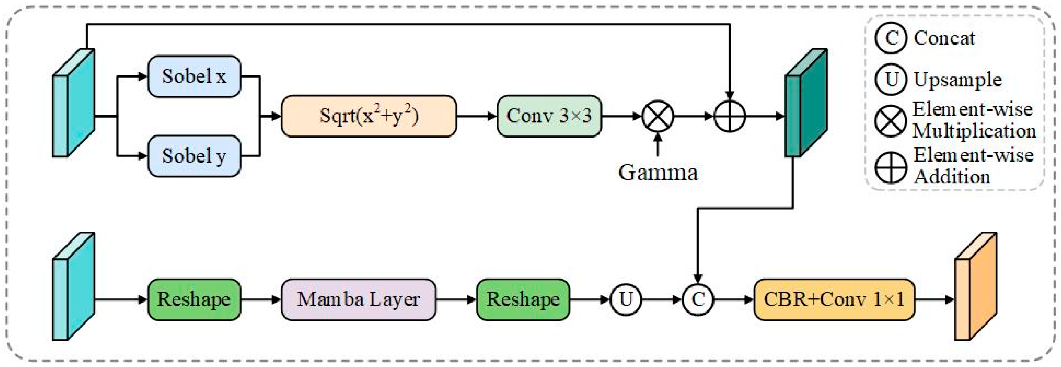
Figure 3.
HBD architecture. The module combines fine-scale edge features enhanced with fixed Sobel gradient operators and learnable enhancement coefficients, and high-level semantic features processed through Mamba sequence modeling. Cross-scale fusion via upsampling integrates enhanced edge features with context-aware representations to generate explicit boundary predictions for camouflaged structure detection.
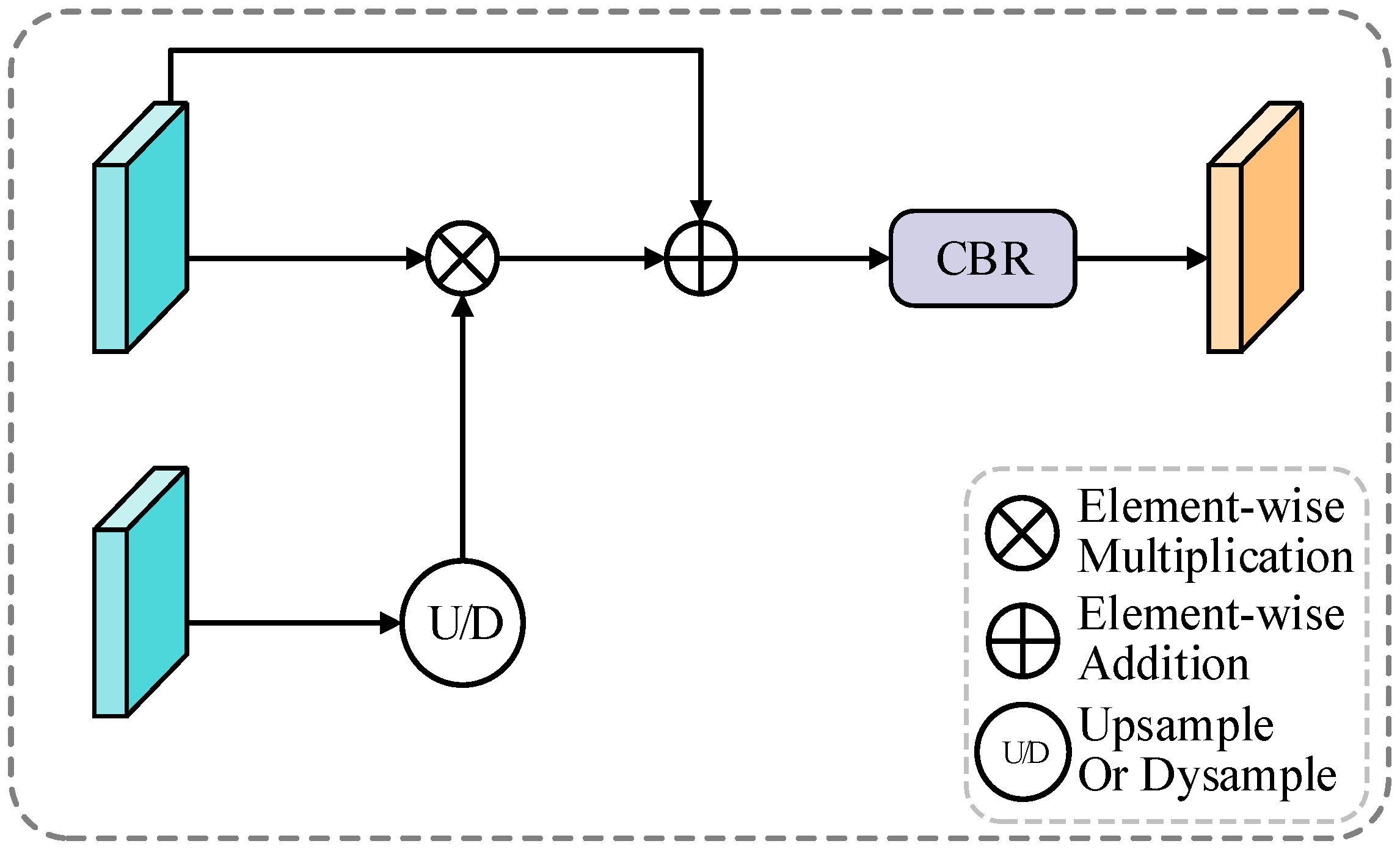
Figure 4.
BGA architecture. The module leverages boundary predictions from HBD to generate attention weights for multi-scale feature enhancement. Boundary attention weights guide feature refinement through interpolation and convolution operations, creating boundary-aware representations for precise edge delineation.
Figure 5.
MFDB architecture. The block combines Mamba’s global sequence modeling pathway (BM-UNet-reshape) with multi-scale MLP local processing using parallel depthwise convolutions (1 × 1, 3 × 3, 5 × 5, 7 × 7). Features are concatenated and processed through ReLU6, dropout, and 1 × 1 convolution, with residual connections ensuring stable gradient flow for boundary-aware reconstruction.
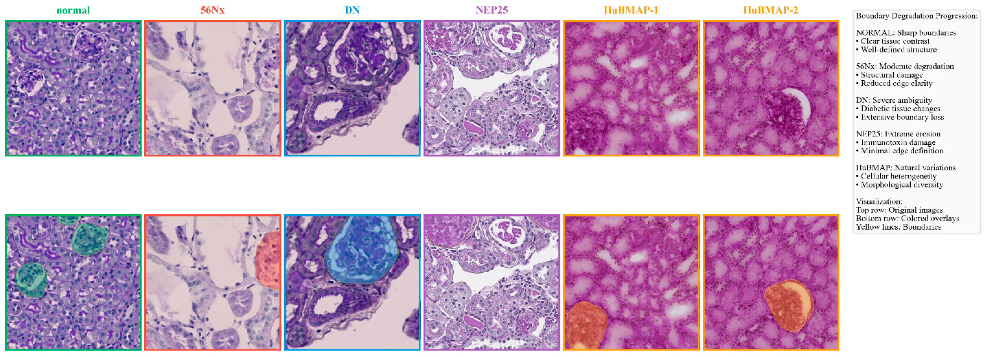
Figure 6.
Dataset visualization demonstrating camouflage challenges. Top row: original images across pathological conditions (Normal, 56Nx, DN, NEP25, HuBMAP-1, and HuBMAP-2). Bottom row: colored overlays highlighting boundary degradation progression.
Figure 6.
Dataset visualization demonstrating camouflage challenges. Top row: original images across pathological conditions (Normal, 56Nx, DN, NEP25, HuBMAP-1, and HuBMAP-2). Bottom row: colored overlays highlighting boundary degradation progression.
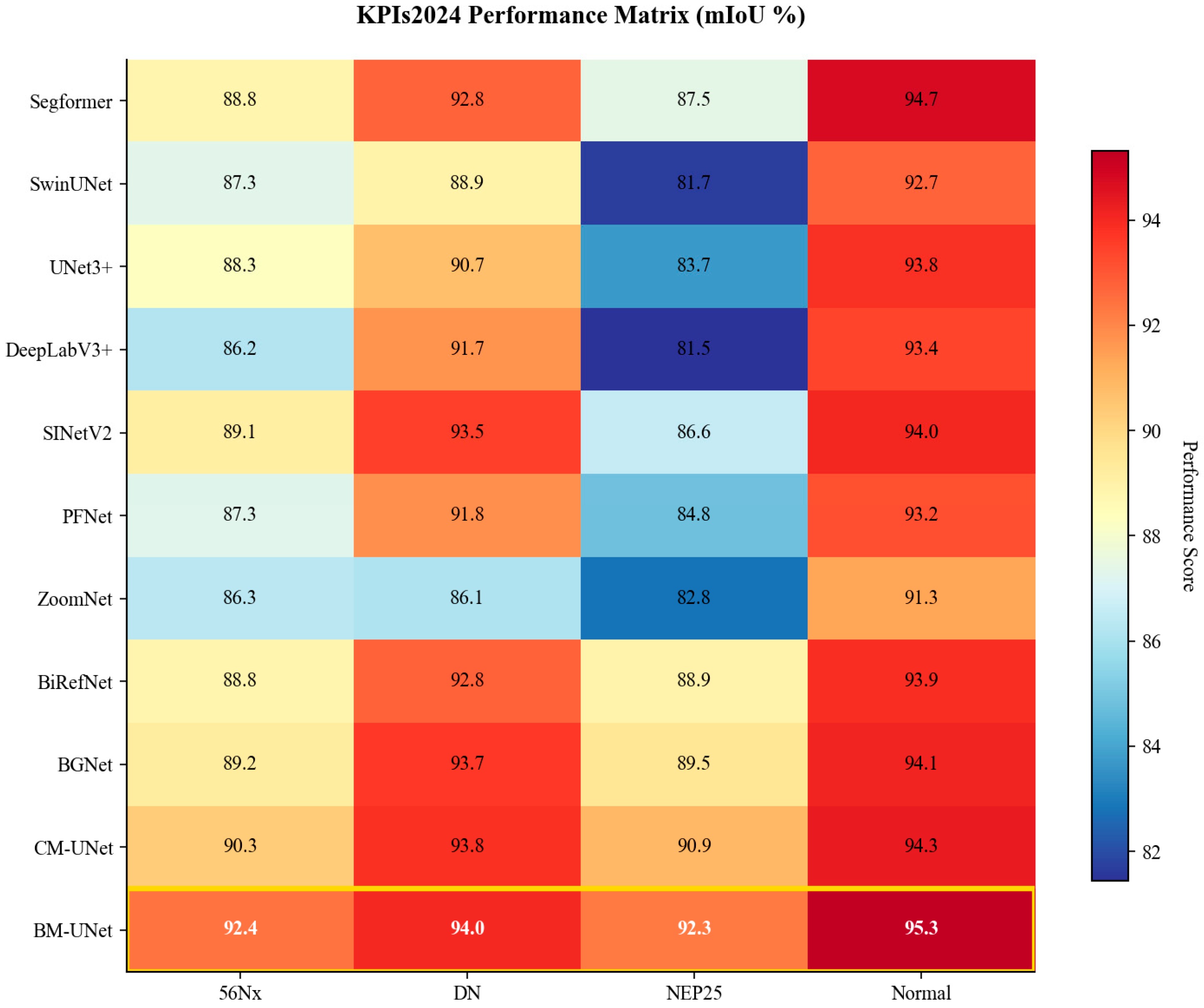
Figure 7.
KPIs2024 performance matrix visualization. Heatmap showing mIoU (%) across all methods and pathological conditions, with color intensity indicating segmentation accuracy.
Figure 7.
KPIs2024 performance matrix visualization. Heatmap showing mIoU (%) across all methods and pathological conditions, with color intensity indicating segmentation accuracy.
Figure 8.
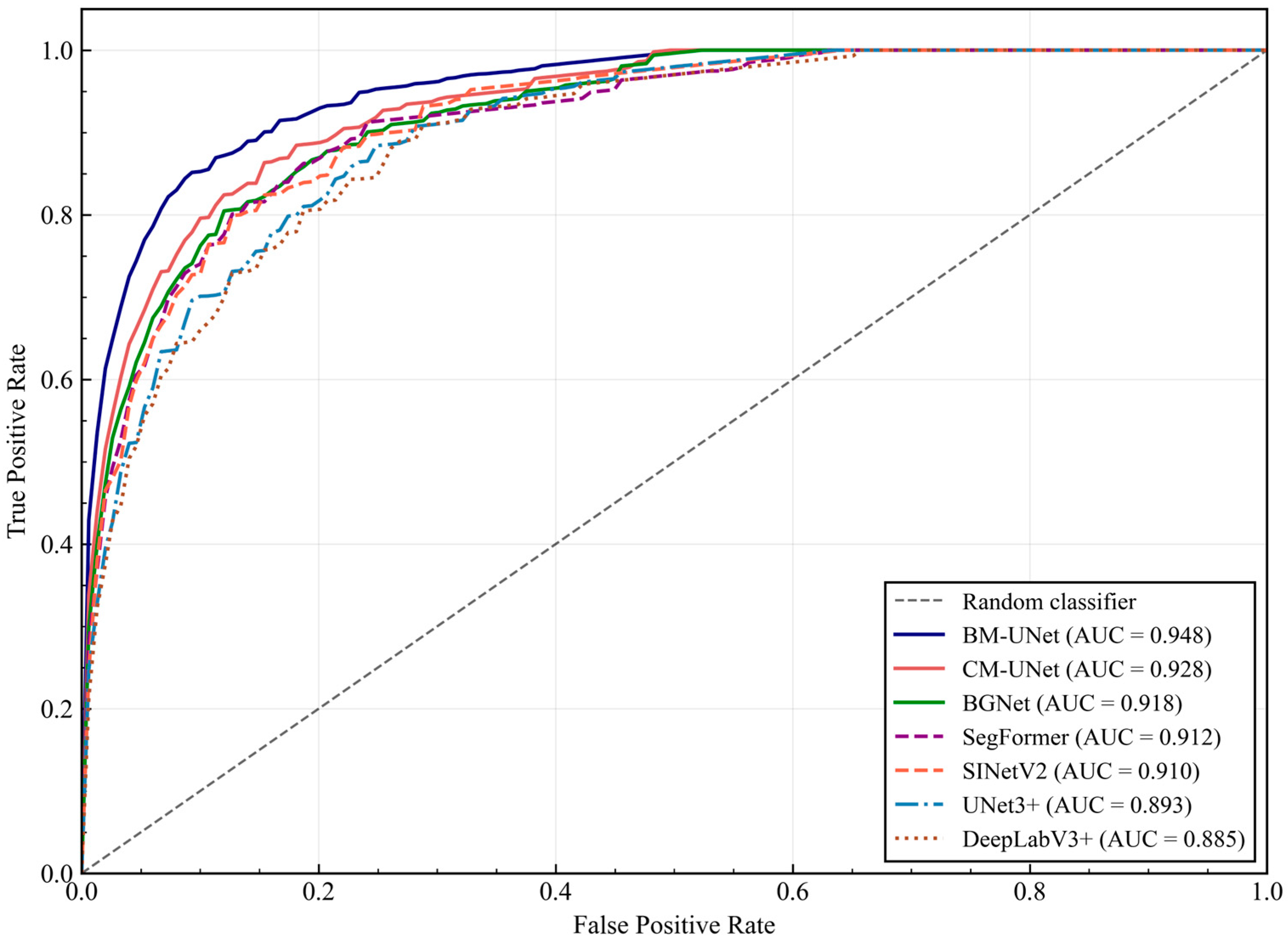
Pixel-wise classification ROC curves for different methods on the KPIs2024 test set. BM-UNet achieves the highest AUC (0.948), demonstrating superior discriminative capability across all operating points. The curves show True Positive Rate vs. False Positive Rate for pixel-wise glomerular classification.
Figure 9.
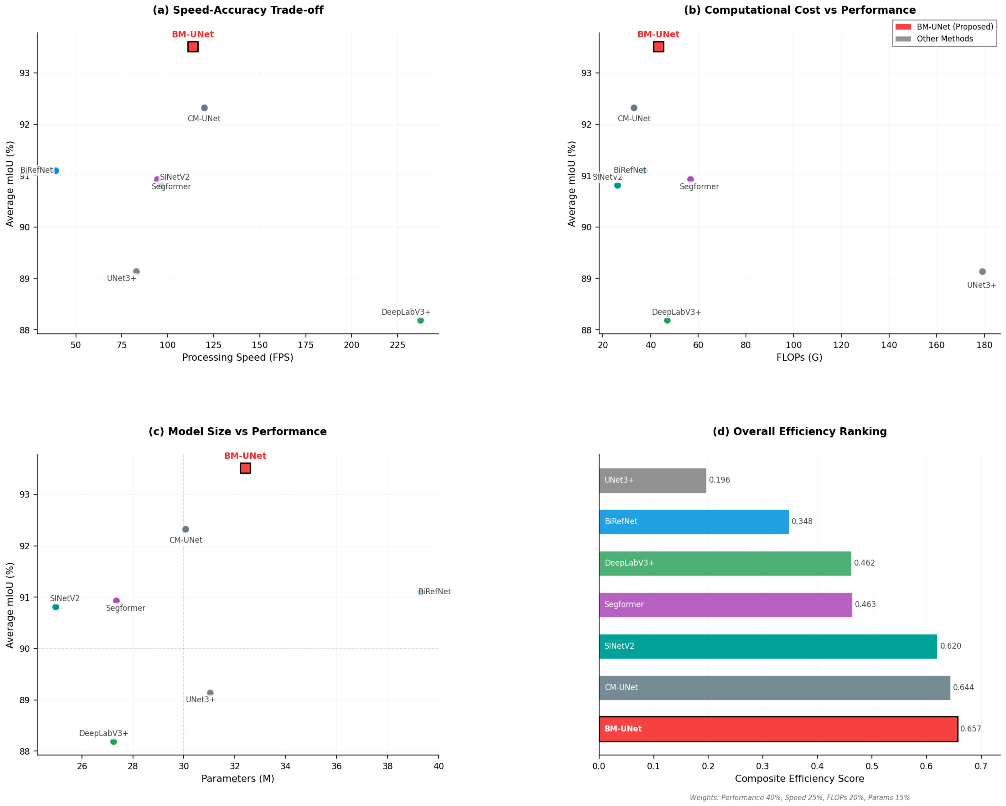
Multi-dimensional performance assessment. (a) Speed–accuracy trade-off; (b) computational cost vs. performance; (c) model size vs. performance; and (d) overall efficiency ranking.
Figure 9.
Multi-dimensional performance assessment. (a) Speed–accuracy trade-off; (b) computational cost vs. performance; (c) model size vs. performance; and (d) overall efficiency ranking.
Figure 10.
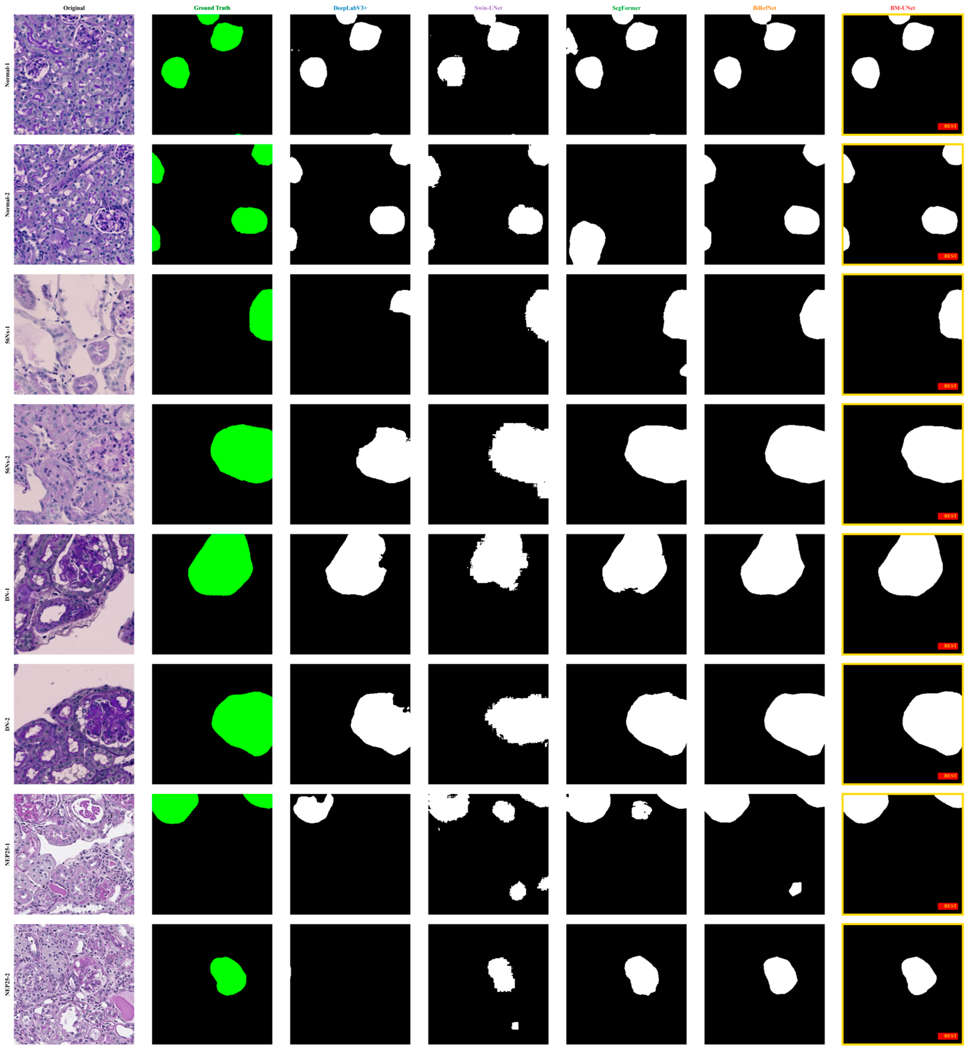
Qualitative segmentation comparison on KPIs2024 dataset. Columns show the original image, ground truth, and results from DeepLabV3+, Swin-UNet, SegFormer, SINetV2, BiRefNet, and BM-UNet. In the ground truth column, the glomerular regions are highlighted in green, while in all model prediction columns, the segmented glomeruli are shown in white against a black background.
Figure 11.
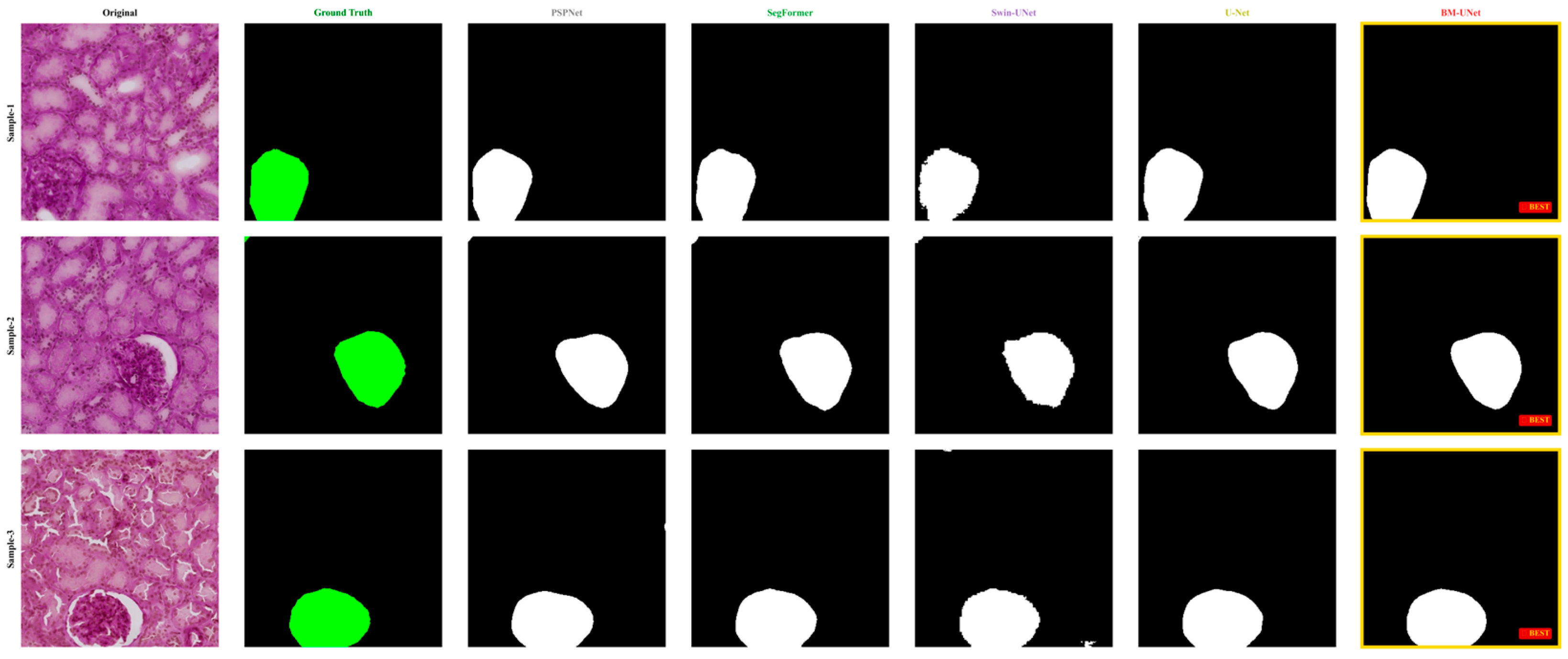
Cross-dataset validation on HuBMAP samples. Segmentation results comparing different methods on human kidney tissue images. In the ground truth column, the glomerular regions are highlighted in green, while in all model prediction columns, the segmented glomeruli are shown in white against a black background.
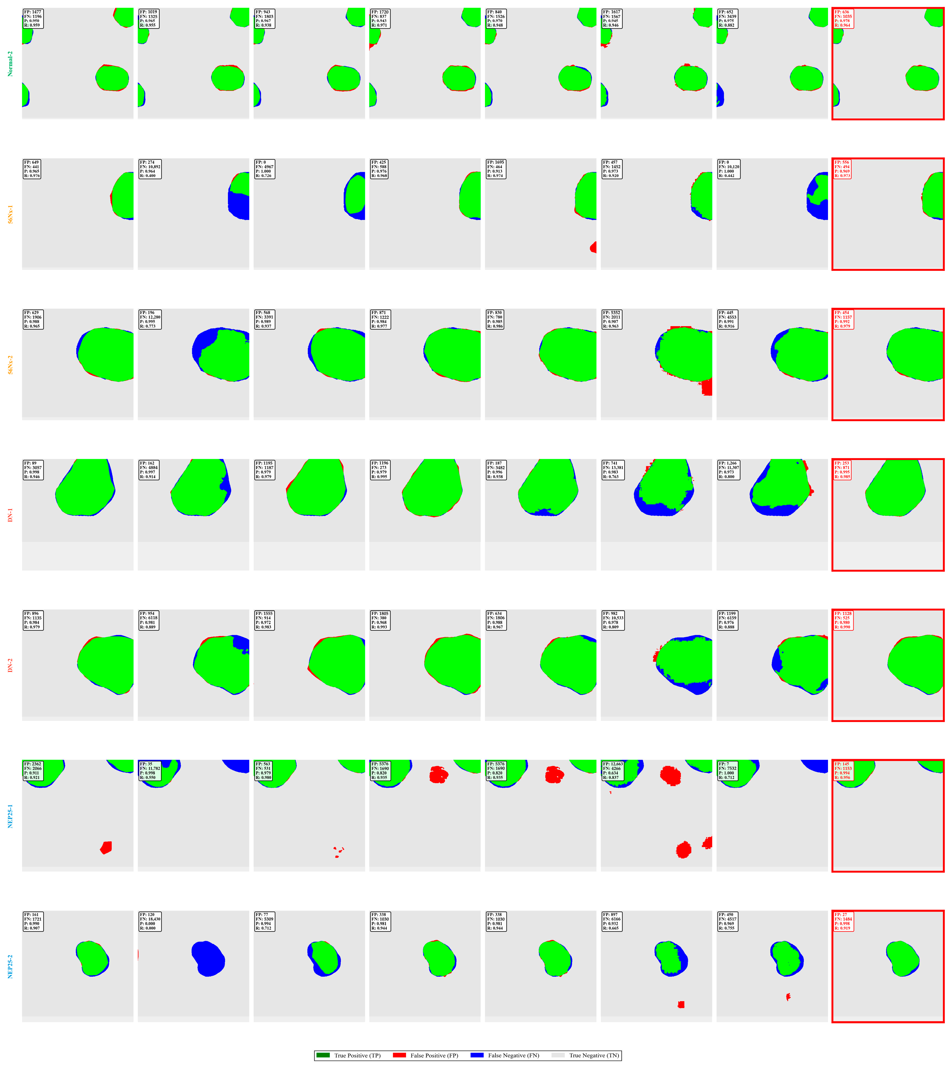
Figure 12.
Comprehensive error analysis visualization. Color-coded error maps: green (TP), red (FP), blue (FN), and gray (TN), with quantitative metrics for each method.
Figure 12.
Comprehensive error analysis visualization. Color-coded error maps: green (TP), red (FP), blue (FN), and gray (TN), with quantitative metrics for each method.
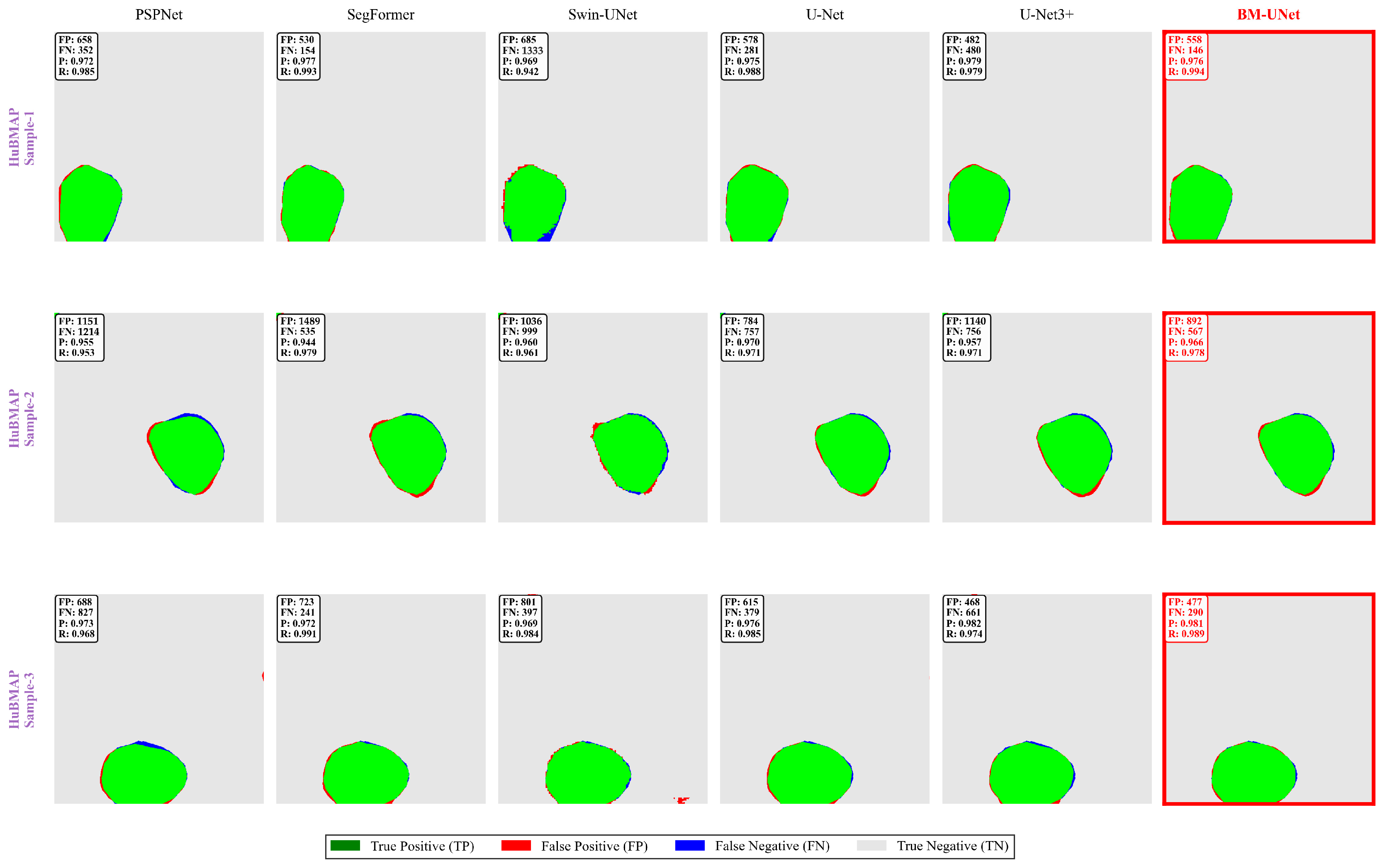
Figure 13.
HuBMAP error analysis. Cross-dataset error validation showing BM-UNet’s superior performance on human tissue samples.
Figure 13.
HuBMAP error analysis. Cross-dataset error validation showing BM-UNet’s superior performance on human tissue samples.
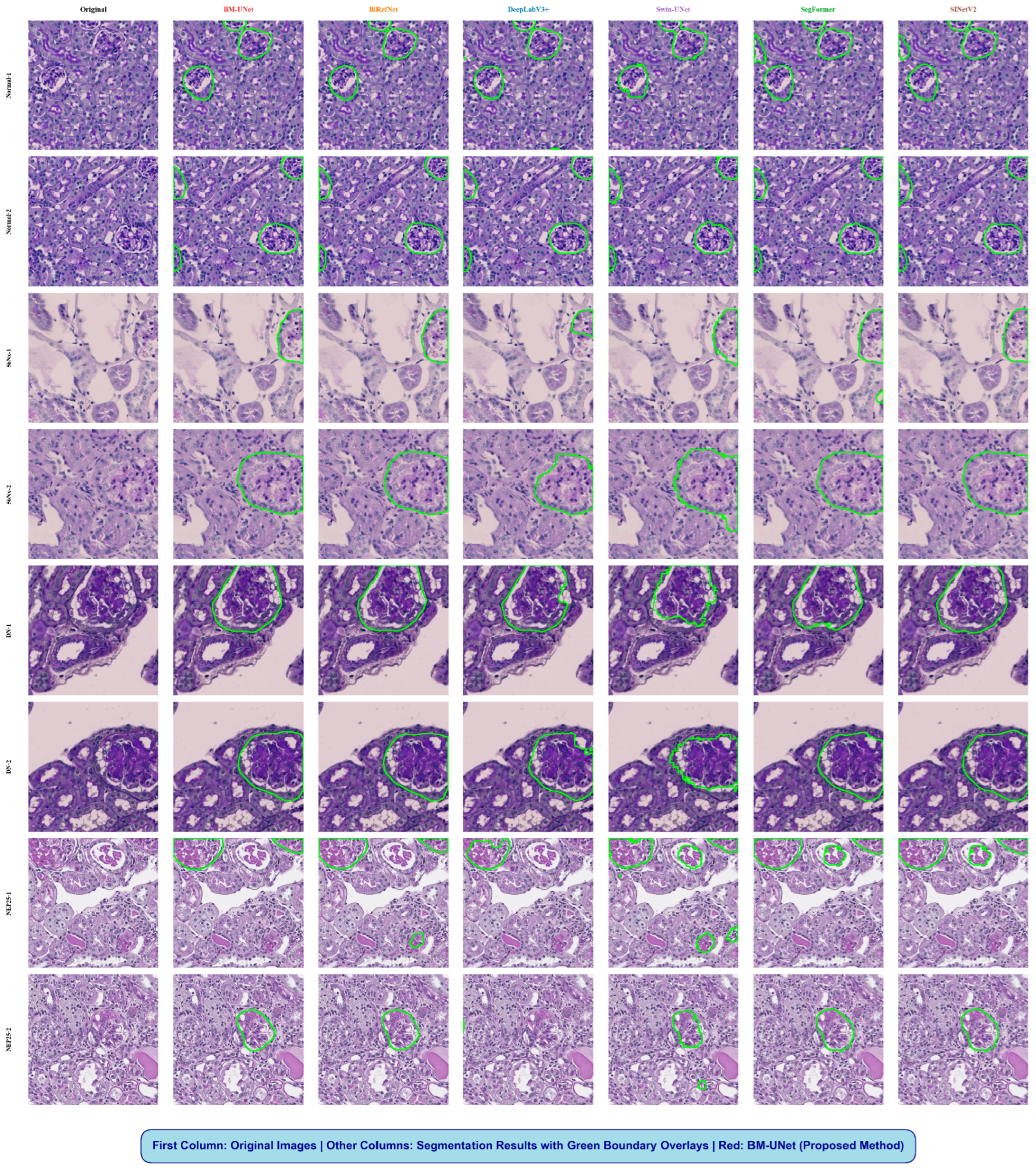
Figure 14.
Boundary overlay analysis. Original histopathological images with segmentation boundary overlays (green contours) across different methods.
Figure 14.
Boundary overlay analysis. Original histopathological images with segmentation boundary overlays (green contours) across different methods.
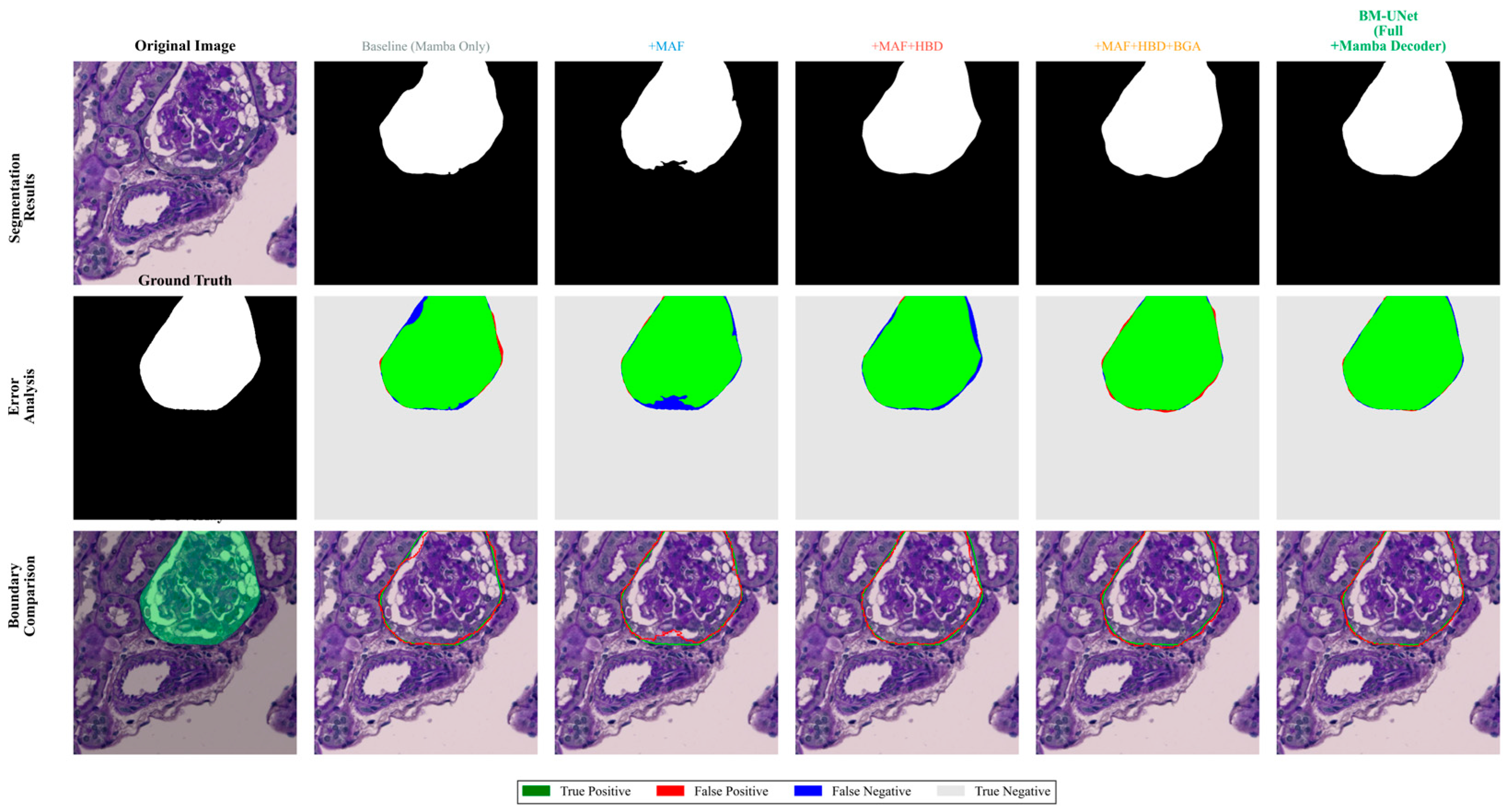
Figure 15.
Progressive ablation study visualization. Top row: segmentation mask evolution; Bottom row: corresponding error analysis through module integration.
Figure 15.
Progressive ablation study visualization. Top row: segmentation mask evolution; Bottom row: corresponding error analysis through module integration.
Figure 16.
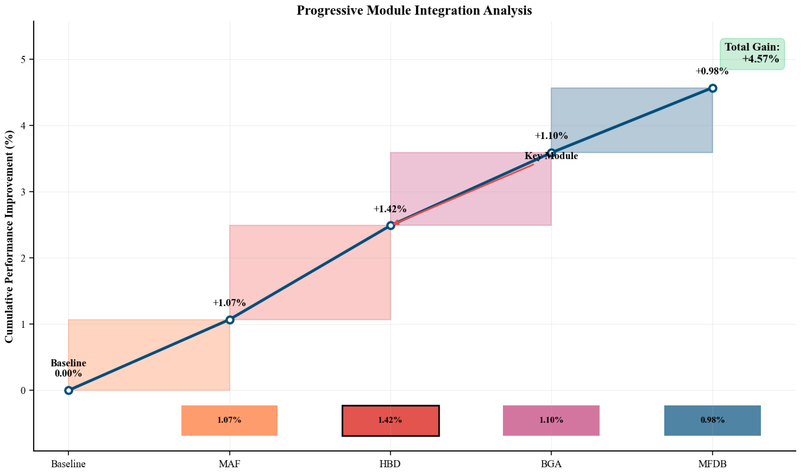
Progressive module integration analysis demonstrating systematic performance improvements through component addition, with boundary-related modules providing the largest contributions for camouflaged structure segmentation.
Figure 16.
Progressive module integration analysis demonstrating systematic performance improvements through component addition, with boundary-related modules providing the largest contributions for camouflaged structure segmentation.
Table 1.
Loss function weight optimization analysis.
Table 1.
Loss function weight optimization analysis.
| λe | Seg mIoU | Boundary mIoU | Training Behavior |
|---|
| 0.1 | 93.72 | 89.84 | Boundary under-optimized |
| 0.3 | 93.64 | 90.67 | Slight improvement |
| 0.5 | 93.51 | 91.34 | Optimal balance |
| 0.7 | 93.28 | 91.52 | Segmentation degradation |
| 0.9 | 92.94 | 91.43 | Over-emphasis on boundaries |
Table 2.
Dataset preprocessing and augmentation pipeline.
Table 2.
Dataset preprocessing and augmentation pipeline.
| Processing Step | Parameters | Application | Dataset Size Impact |
|---|
| Image Resizing | 512 × 512 pixels | All images | No change |
| Random Horizontal Flip | Probability p = 0.5 | Training only | Online augmentation |
| Random Vertical Flip | Probability p = 0.5 | Training only | Online augmentation |
| Random Cropping | Dynamic crop after resizing | Training only | Online augmentation |
| ImageNet Normalization | μ = [0.485, 0.456, 0.406];
σ = [0.229, 0.224, 0.225] | All images | No change |
Table 3.
KPIs2024 dataset composition and characteristics.
Table 3.
KPIs2024 dataset composition and characteristics.
| Condition | Resolution | Training | Test | Total | Disease Model | Staining |
|---|
| Normal | 512 × 512 | 980 | 327 | 1307 | Healthy control | PAS |
| 56Nx | 512 × 512 | 979 | 327 | 1306 | 5/6 nephrectomy | PAS |
| DN | 512 × 512 | 975 | 325 | 1300 | Diabetic model | PAS |
| NEP25 | 512 × 512 | 976 | 325 | 1301 | Podocyte injury | PAS |
| Total | 512 × 512 | 3910 | 1304 | 5214 | 4 models | PAS |
Table 4.
HuBMAP dataset specifications.
Table 4.
HuBMAP dataset specifications.
| Split | Resolution | Count | Content | Annotation |
|---|
| Training | 512 × 512 | 2576 | Human kidney | Expert |
| Test | 512 × 512 | 1104 | Human kidney | Expert |
| Total | 512 × 512 | 3680 | PAS-stained | Manual |
Table 5.
Quantitative performance comparison on KPIs2024 dataset with statistical significance analysis.
Table 5.
Quantitative performance comparison on KPIs2024 dataset with statistical significance analysis.
| Model Variant | Architecture | 56Nx | DN | NEP25 | Normal | Avg mIoU | Std | p-Value † |
|---|
| U-Net | CNN | 85.12 ± 0.48 | 88.34 ± 0.42 | 80.56 ± 0.54 | 91.78 ± 0.35 | 86.45 | 4.82 | <0.001 *** |
| PSPNet | CNN | 85.89 ± 0.46 | 89.72 ± 0.41 | 81.93 ± 0.52 | 92.35 ± 0.33 | 87.47 | 4.51 | <0.001 *** |
| DeepLabV3+ | CNN | 86.19 ± 0.47 | 91.70 ± 0.39 | 81.45 ± 0.51 | 93.42 ± 0.31 | 88.19 | 5.45 | <0.001 *** |
| UNet3+ | CNN | 88.32 ± 0.42 | 90.71 ± 0.40 | 83.73 ± 0.49 | 93.81 ± 0.30 | 89.14 | 4.25 | <0.001 *** |
| ConvNeXt | CNN | 88.45 ± 0.41 | 91.23 ± 0.38 | 85.79 ± 0.47 | 93.28 ± 0.29 | 89.69 | 3.12 | <0.001 *** |
| Segformer | Transformer | 88.77 ± 0.39 | 92.77 ± 0.37 | 87.45 ± 0.44 | 94.73 ± 0.27 | 90.93 | 3.40 | 0.008 ** |
| SwinUNet | Transformer | 87.34 ± 0.45 | 88.89 ± 0.43 | 81.72 ± 0.53 | 92.72 ± 0.32 | 87.67 | 4.56 | <0.001 *** |
| SINetV2 | COD | 89.13 ± 0.38 | 93.53 ± 0.35 | 86.57 ± 0.43 | 94.04 ± 0.26 | 90.82 | 3.59 | 0.011 * |
| PFNet | COD | 87.27 ± 0.43 | 91.85 ± 0.39 | 84.84 ± 0.48 | 93.17 ± 0.30 | 89.78 | 3.97 | <0.001 *** |
| ZoomNet | COD | 86.34 ± 0.47 | 86.14 ± 0.50 | 82.81 ± 0.52 | 91.35 ± 0.34 | 86.66 | 3.70 | <0.001 *** |
| BiRefNet | COD | 88.81 ± 0.37 | 92.82 ± 0.34 | 88.89 ± 0.42 | 93.87 ± 0.25 | 91.10 | 2.24 | 0.026 * |
| BGNet | COD | 89.23 ± 0.36 | 93.67 ± 0.33 | 89.49 ± 0.40 | 94.11 ± 0.24 | 91.63 | 2.47 | 0.042 * |
| CM-UNet | Mamba | 90.29 ± 0.33 | 93.81 ± 0.31 | 90.87 ± 0.38 | 94.34 ± 0.23 | 92.33 | 1.72 | 0.049 * |
| BM-UNet (ours) | COD-Mamba | 92.43 ± 0.29 | 94.02 ± 0.28 | 92.28 ± 0.35 | 95.32 ± 0.21 | 93.51 | 1.34 | - |
Table 6.
Cross-dataset validation on HuBMAP dataset with statistical significance.
Table 6.
Cross-dataset validation on HuBMAP dataset with statistical significance.
| Model Variant | Architecture | mPA (%) | mIoU (%) | mDice (%) | p-Value † |
|---|
| U-Net | CNN | 96.12 ± 0.13 | 93.57 ± 0.18 | 96.71 ± 0.11 | <0.001 *** |
| UNet3+ | CNN | 96.48 ± 0.12 | 93.68 ± 0.17 | 96.77 ± 0.10 | <0.001 *** |
| PSPNet | CNN | 95.52 ± 0.15 | 93.12 ± 0.20 | 96.49 ± 0.12 | <0.001 *** |
| DeepLabV3plus | CNN | 96.25 ± 0.13 | 93.45 ± 0.18 | 96.72 ± 0.11 | <0.001 *** |
| ConvNeXt | CNN | 96.78 ± 0.11 | 93.85 ± 0.16 | 96.81 ± 0.09 | 0.034 * |
| Segformer | Transformer | 96.55 ± 0.12 | 93.89 ± 0.16 | 96.89 ± 0.09 | 0.046 * |
| SwinUNet | Transformer | 95.23 ± 0.16 | 92.43 ± 0.21 | 96.15 ± 0.13 | <0.001 *** |
| BM-UNet (ours) | COD-Mamba | 97.12 ± 0.10 | 94.32 ± 0.15 | 97.19 ± 0.08 | - |
Table 7.
Computational efficiency analysis comparing processing speed and resource requirements.
Table 7.
Computational efficiency analysis comparing processing speed and resource requirements.
| Method | FLOPs (G) | Params (M) | FPS |
|---|
| DeepLabV3plus | 46.94 | 27.23 | 237.4 |
| Swin-UNet | 30.92 | 27.15 | 121.1 |
| U-Net3+ | 179.08 | 31.03 | 82.8 |
| Segformer | 56.71 | 27.35 | 94.3 |
| SINetV2 | 26.11 | 24.96 | 96.2 |
| BiRefNet | 37.4 | 39.29 | 38.9 |
| CM-UNet | 33.05 | 30.07 | 119.7 |
| BM-UNet (ours) | 43.31 | 32.42 | 113.7 |
Table 8.
Clinical deployment validation across different hardware platforms.
Table 8.
Clinical deployment validation across different hardware platforms.
| Hardware Platform | Peak Memory
Usage (GB) | Total Processing Time (s) | Avg. Time per Image (ms) | Throughput
(Images/s) |
|---|
| NVIDIA RTX 4090 (24 GB) | 2.3 | 1.76 | 8.8 | 113.6 |
| NVIDIA RTX 3060 (12 GB) | 2.3 | 3.08 | 15.4 | 64.9 |
| NVIDIA RTX 2070 (8 GB) | 2.3 | 4.12 | 20.6 | 48.5 |
| NVIDIA GTX 1660 Ti (6 GB) | 2.3 | 8.62 | 43.1 | 23.2 |
Table 9.
Comprehensive ablation study demonstrating the contribution of each BM-UNet component across multiple evaluation metrics.
Table 9.
Comprehensive ablation study demonstrating the contribution of each BM-UNet component across multiple evaluation metrics.
| Method | 56Nx | DN | NEP25 | Normal |
|---|
| mIoU | mDice | mPA | mIoU | mDice | mPA | mIoU | mDice | mPA | mIoU | mDice | mPA |
|---|
| Baseline (Mamba Only) | 87.8 | 90.2 | 92.5 | 89.51 | 91.8 | 93.8 | 87.47 | 89.9 | 92.1 | 90.94 | 93.1 | 94.2 |
| +MAF | 88.9 | 91.3 | 93.4 | 90.54 | 92.9 | 94.6 | 88.96 | 91.4 | 93.2 | 91.59 | 93.9 | 94.8 |
| +MAF + HBD | 90.3 | 92.8 | 94.7 | 91.64 | 94.1 | 95.3 | 90.25 | 92.7 | 94.5 | 93.49 | 95.2 | 96.1 |
| +MAF + HBD + BGA | 91.5 | 93.9 | 95.4 | 92.99 | 95.3 | 96.1 | 91.50 | 93.8 | 95.3 | 94.09 | 95.7 | 96.5 |
| BM-UNet (Full + MFDB) | 92.43 | 94.7 | 96.1 | 94.02 | 96.2 | 96.8 | 92.28 | 94.6 | 96.0 | 95.32 | 96.9 | 97.2 |


