Article

Transformer-Driven GAN for High-Fidelity Edge Clutter Generation with Spatiotemporal Joint Perception

by
Xiaoya Zhao
1,
Junbin Ren
1,
Wei Tao
1,
Anqi Chen
1,
Xu Liu
2,
Chao Wu
1,*,
Cheng Ji
1,*,
Mingliang Zhou
3 and
Xueyong Xu
4
1
School of Computer Science and Engineering, Nanjing University of Science and Technology, Nanjing 210094, China
2
Academy of Advanced Interdisciplinary Research, Xidian University, Xi’an 710126, China
3
School of Computer Science, Chongqing University, Chongqing 400044, China
4
North Information Control Research Academy Group Company Limited, Nanjing 211100, China
*
Authors to whom correspondence should be addressed.
Symmetry 2025, 17(9), 1489; https://doi.org/10.3390/sym17091489
Submission received: 2 July 2025 / Revised: 14 August 2025 / Accepted: 18 August 2025 / Published: 9 September 2025
(This article belongs to the Special Issue Symmetry and Asymmetry in Embedded Systems)

Abstract

Accurate sea clutter modeling is crucial for clutter suppression in edge radar processing. On resource-constrained edge radar platforms, spatiotemporal statistics, together with device-level computation and memory limits, hinder the learning of representative clutter features. This study presents a transformer-based generative adversarial model for sea clutter modeling. The core design of this work uses axial attention to factorize self-attention along pulse and range, preserving long-range dependencies under a reduced attention cost. It also introduces a two-dimensional variable-length spatiotemporal window that retains temporal and spatial coherence across observation lengths. Extensive experiments are conducted to verify the efficacy of the proposed method with quantitative criteria, including a cosine similarity score, spectral-parameter error, and amplitude–distribution distances. Compared with CNN-based GAN, the proposed model achieves a high consistency with real clutter in marginal amplitude distributions, spectral characteristics, and spatiotemporal correlation patterns, while incurring a lower cost than standard multi-head self-attention. The experimental results show that the proposed method achieves improvements of 9.22% and 7.8% over the traditional AR and WaveGAN methods in terms of the similarity metric, respectively.

1. Introduction

Sea clutter is an unwanted radar return produced by backscatter from an object’s surface [1]. It is a type of interference in real-time signal processing applications, e.g., clutter modeling and suppression in the sea edge environment. The clutter strength depends on several variables, including the weather and fluctuations in wind and waves. Sea surface target identification is significantly hampered by the unexpected nature of sea clutter in complicated ocean environments. Understanding sea clutter features and investigating target identification techniques require high-quality sea clutter data. Currently, there are two main ways to obtain sea clutter information: (1) field measurements: onsite measurements are used to obtain data on actual sea clutter. (2) Theoretical modeling and simulation: recent advances have introduced neural networks to rapidly select preferential statistical distributions for sea clutter modeling [2], while Spatiotemporal Graph Neural Networks (ST-GNNs) demonstrate efficacy in capturing multivariate dependencies for time-series forecasting—a framework adaptable to sea clutter dynamics [3]. Sea clutter usually exhibits asymmetric spatial and temporal features. Traditional modeling methods primarily employ two methodologies: the first method builds an echo sequence model based on sea surface models and electromagnetic scattering concepts, and the second technique involves applying classical statistical models to fit sea clutter amplitudes [4], typically using Zero-Memory Nonlinear (ZMNL) transformation and Spherically Invariant Random Process (SIRP) [5,6].
Field measurements remain paramount in investigating sea clutter characteristics. However, these experiments require significant time and financial resources, along with confidentiality constraints that limit data accessibility [7]. Conventional modeling approaches often oversimplify the non-Gaussian and non-stationary properties of sea clutter [8], resulting in simulated data with limited precision and practical value. The challenge of obtaining high-quality, diverse sea clutter data persists as a key research focus in sea surface target detection [9].
Owing to the limitations of traditional clutter signal modeling approaches, recent breakthroughs using generative adversarial networks (GANs) for radar data generation [10,11] further highlight the potential of deep learning in addressing these limitations. Through adversarial training, GANs have achieved remarkable success in the generation of images and musical compositions [12,13,14], and they have also demonstrated the promising potential of generating radar data. Jing et al. introduced a deep learning model named the adversarial extrapolation neural network (AENN) [15]. By leveraging the GAN architecture, this model addresses the challenge of generating weather radar echo data through extrapolation. Importantly, the use of adversarial training in AENN effectively addresses the problem of ambiguous predictions. This technique can generate precise and convincing extrapolation echoes for weather radar data. Another study uses a Wasserstein GAN structure to synthesize radar waveforms from complex-valued radar data [16], showing that their approach may generate new waveforms with shapes that are substantially comparable to the actual data. The authors of [17] designed a novel GAN model to generate radar signals. Three concealed object classes are used as training data. The designed WaveGAN can synthesize radar signal data that are indistinguishable from the training data via qualitative analysis conducted by human observers. Furthermore, WaveGAN is used to simulate radar clutter, and the generated data are assessed via the maximum mean discrepancy (MMD) approach [18,19]. Semi-supervised generative adversarial networks (GANs) further address challenges in sea–land clutter classification, particularly in over-the-horizon radar systems, by mitigating labeled data scarcity through weighted-loss architectures [20].
Although the above works can partially address the problems of conventional methods, they mostly rely on convolutional neural networks (CNNs) and can only have a limited capacity for feature extraction of sea clutter data, which is a type of discrete multidimensional time series data [21]. Recurrent neural network (RNN)-based models are frequently employed for time series data modeling; nevertheless, we argue that the transformer model is a better option, given the possibility of information loss during computation in RNNs and related models. Compared with conventional CNN and RNN models, the transformer model offers better flexibility and expressive power in sequence modeling and is good at capturing long-range dependencies between sequences, which improves the understanding and processing of the distinctive elements in the data from sea clutter. Given that clutter exhibits strong sequential and spatial features, this work exploits the advantages of transformer networks to effectively realize feature extraction and generate sea clutter data. The self-attention mechanism can capture dependencies between elements in sequence data, which is beneficial for retaining the dynamic information in sea clutter data. Additionally, positional encoding techniques help the model understand the sequence data’s order and spatial relationships, further enhancing the model’s ability to handle sea clutter data.
In comparing sea clutter and target feature distributions, KL divergence measures overall differences but is sensitive to zero-probability regions and non-symmetry, leading to bias in high-dimensional sparse spaces [22]; the KS distance focuses on the maximum deviation between empirical cumulative distributions but neglects differences elsewhere and yields unstable significance under small-sample conditions, lacking directional information [23]. Spectral parameter error has long been used to quantify the fitting accuracy of Doppler peak location and spectral width [24]; amplitude distribution distances (such as Bhattacharyya and Hellinger distances) are standard metrics for evaluating heavy-tailed sea clutter amplitude model fit [25]. Under extreme sea states or multi-polarization mixed echoes, conventional metrics, such as the Kullback–Leibler divergence and the Kolmogorov—Smirnov distance, exhibit insufficient sensitivity to long-tailed distributions and phase characteristics, thereby failing to comprehensively characterize the statistical discrepancies of the generated echoes. The studies by Vondra B [26] and Wen B [27], respectively, demonstrate that, in high-dynamic-range sea clutter scenarios, traditional amplitude distribution distances and simple spectral error metrics are prone to false negatives and false positives. This paper introduces the similarity (Sim) metric based on cosine similarity, which directly measures the angle between high-dimensional feature vectors without density estimation, provides a unified evaluation across time-domain and frequency-domain features, and offers a novel, efficient tool for performance assessment in small-sample, high-dimensional generated data quality checks [28].
In summary, this study introduces a novel method for generating sea clutter data by combining transformer and generative adversarial network (GAN) architectures. The main contributions of this study are as follows:
  • An approach for extracting spatiotemporal features from generated sea clutter data via a transformer network and a GAN is proposed. Specifically, by employing axial attention in place of traditional attention mechanisms, we effectively extract long-range spatiotemporal dynamic information from sea clutter data.
  • We propose a technique for creating and using two-dimensional variable-length vectors to maintain the spatiotemporal properties of sea clutter data, improving the realism of the generated samples.
  • We conducted qualitative and quantitative experiments to assess the quality of the generated data in comparison with real data and traditional, other GAN-based, mainstream clutter generation methods, confirming the superior accuracy of the proposed approach.
In recent years, sea clutter generation and detection have seen huge progress in classical radar signal processing and deep generative modeling. Foundational treatments in Skolnik’s Radar Handbook formalized pulse-compression waveforms and CFAR processors [29], while Greco and Gini’s statistical analysis of high-resolution SAR ground clutter introduced parametric priors for amplitude modeling [30]. Building on these foundations, Smith et al. combined dynamic time warping with convolutional neural networks for micro-Doppler classification [31], and Li et al. developed a convolutional ResNet that improved small-boat target-to-clutter SNR in maritime scenes [32]. On the generative side, Wang et al. demonstrated GAN-based speckle restoration for SAR imagery [33], and Yang et al. employed diffusion models to jointly synthesize time- and frequency-domain clutter representations [34]. The above approach motivates the design of our spatial-temporal joint perception GAN, which couples long-range temporal dependencies with spectral–amplitude consistency for edge-end clutter generation.
The remainder of the paper is organized as follows. The fundamental principles of generative adversarial networks (GANs), transformer networks, and the characteristics of sea clutter are described in Section 2. We introduce our dataset and novel method in Section 3. In addition, we provide the parameter settings and training details. We present the experiments that were performed and the evaluation findings in Section 4. We summarize our work and conclude this paper in Section 5.

2. Background

2.1. Generative Adversarial Network

Goodfellow et al. proposed the generative adversarial network (GAN) [9] as a revolutionary network paradigm in 2014. In the conventional GAN design for generating the data shown in Figure 1, the model is divided into two parts: the generator (G) and the discriminator (D). The discriminator is a binary classifier that attempts to differentiate between actual and produced data. The generator, on the other hand, seeks to generate samples that are as close to the real-world data as possible to deceive the discriminator.
When the labels for real and produced samples are 1 and 0, respectively, the GANs rely on a minimax game, with the optimization function stated as follows:
min G max D V ( D , G ) = E x P d a t a ( x ) [ log D ( x ) ] + E z P z ( z ) [ log ( 1 D ( G ( z ) ) ) ] .
Here, x represents real data samples, and z is a random noise vector from a prior distribution P z ( z ) . While the discriminator strives to precisely discriminate between real and created data, the generator’s objective is to produce samples that are indistinguishable from real data. The generator and discriminator compete with one another repeatedly until a Nash equilibrium is established in the optimization process. Generative adversarial networks (GANs) suffer from the issue of training instability. The Wasserstein GAN with gradient penalty (WGAN–GP) [35] was proposed, which improves the stability of GAN training by modifying the GAN loss function.
Other works have concentrated on strengthening network designs to increase GAN performance. The self-attention GAN (SAGAN) [36], for instance, adds self-attention mechanisms to GANs, creating long-range dependencies and improving the quality of generated data. Indeed, combining attention mechanisms with GANs has proven to be highly effective. These works provide an essential foundation and inspiration for this study.

2.2. Transformer

The transformer network consists of an encoder and a decoder that are both made up of completely coupled feedforward networks and attention processes. The transformer model effectively captures dependencies and contextual information within sequence data and relies heavily on the self-attention process. Queries (Q), keys (K), and values (V) are three sets of vectors, and their relationships are defined as follows:
A t t e n t i o n ( Q , K , V ) = s o f t m a x ( Q K T d ) V .
Here, Q, K, and Q are matrices representing the queries, keys, and values, respectively. d is the dimensionality of the key vectors.
A transformer-based GAN was used to produce images in prior works [37,38], with promising results. Reference [39] employed a GAN composed of transformer networks to generate time series sequences and verified its practicality on datasets such as the PTB diagnostic ECG. Additionally, the application of transformer-based GANs for time series prediction has shown promising performance in various tasks, including long-term human motion prediction, anomaly detection, and pedestrian trajectory prediction [40,41,42]. These works demonstrate the effectiveness of combining the transformer network with GANs, delivering notable performance improvements in both the temporal and spatial dimensions.

2.3. Characteristics of Radar Clutter

Amplitude characteristics: The echo signals from scattering substances and various scatter centers conflict with one another when a radar beam illuminates a given area, causing considerable changes in signal amplitude (abs). The probability density distribution is frequently analyzed, and statistical models are utilized to describe the clutter amplitude characteristics [1].
Doppler characteristics: The Fourier transform of the autocorrelation function of the time series signal within a single radar resolution cell is referred to as the Doppler spectrum of sea clutter. To investigate the spectral shape, bandwidth, and mean Doppler frequency shift of the radar, a Gaussian spectrum model is commonly used to analyze the radar’s Doppler characteristics [24,43].
Temporal correlation characteristics: The correlation between radar echoes from the sea surface received at different pulse times is referred to as the sea clutter temporal correlation. It is most often studied by means of the normalized autocorrelation function or autocorrelation coefficient. Let the complex sea clutter echo at the n-th pulse be denoted by r ( n ) . The theoretical autocorrelation coefficient between r ( n ) and r ( n + l ) is defined as
ρ n , n + l = E r ( n ) , r ( n + l ) E r ( n ) , E r ( n + l ) Var [ r ( n ) ] Var [ r ( n + l ) ] ,
where E [ · ] denotes statistical expectation, * denotes complex conjugation, and
Var [ r ( n ) ] = E | r ( n ) | 2 E [ r ( n ) ] 2
is the variance of the clutter amplitude at the n-th pulse. In practice, assuming wide-sense stationarity of the sea clutter process over a short burst of N pulses, one uses the sample estimator
ρ n , n + l = E r ( n ) r * ( n + l ) E r ( n ) E r * ( n + l ) Var [ r ( n ) ] Var [ r ( n + l ) ]
where
r ¯ = 1 N n = 0 N 1 r ( n ) , | r | 2 ¯ = 1 N n = 0 N 1 | r ( n ) | 2
and the denominator | r | 2 ¯ | r ¯ | 2 equals the sample variance of r ( n ) . The normalized autocorrelation coefficient ρ ( l ) lies in the interval [ 1 , 1 ] , with ρ ( 0 ) = 1 . As the pulse lag l increases, ρ ( l ) typically exhibits a rapid decay. The delay l corr at which ρ ( l ) falls to 1 / e 0.368 is taken to define the clutter correlation time scale; converting to physical time gives the following:
T corr = l corr × PRI
where PRI is the pulse repetition interval. At lags beyond l corr , the sea clutter echoes may be regarded as being effectively uncorrelated in time.
Spatial correlation characteristics: The amplitude correlation of the radar signals backscattered from the sea surface at radially dispersed distance units is referred to as the sea clutter spatial correlation. Autocorrelation functions or spatial correlation coefficients are mostly used to study this phenomenon. The spatial autocorrelation coefficient between x ( k ) and x ( k + l ) is defined as follows if the sea clutter sequence of the k-th distance unit is represented as x ( k ) :
p k , k + l = E [ x ( k ) x * ( k + l ) ] E [ x ( k ) ] E [ x * ( k + l ) ] σ [ x ( k ) ] σ [ x ( k + l ) ] .
Here, σ is the variance, and ∗ denotes the complex conjugate. Assuming that sea clutter is spatially uniform within a short distance, we can use the correlation coefficient estimation formula:
p ( l ) = 1 N k = 0 N l 1 x ( k ) x * ( k + l ) | x ¯ | 2 | x 2 | ¯ | x ¯ | 2 .
where p ( l ) can take values ranging from −1 to +1. Initially, when displaying a reasonably high correlation, the correlation coefficient p ( l ) between adjacent units of x ( k ) then goes through a quick decay process. When p ( l ) falls from 1 to 1 / e (approximately 0.368), it is assumed that the sea clutter is no longer associated with the distance direction. At this point, the number of distance units represents the correlation length.

2.4. Evaluation Metrics in Sea Clutter Generation

In sea clutter generation, appropriate metrics are essential, yet conventional choices often fail or become biased under complex sea states and multi-polarization settings, making comprehensive assessment difficult. This section (i) reviews the limitations of traditional metrics, (ii) introduces our cosine similarity-based Sim metric over multi-moment feature vectors, and (iii) proves its effectiveness from sufficiency and necessity perspectives.

2.4.1. Limitations of Traditional Metrics

Amplitude–distribution distances (KL/KS/JS).
D KL ( P Q ) = i P ( i ) log P ( i ) Q ( i ) , D KS ( P , Q ) = sup x F P ( x ) F Q ( x ) .
The Jensen–Shannon distance is
D JS ( P Q ) = 1 2 D KL ( P M ) + 1 2 D KL ( Q M ) , M = 1 2 ( P + Q ) .
Although symmetric and more stable than KL [44], JS may still under-react to extreme-amplitude variability in high–dynamic-range, multimodal heavy-tailed regimes [45].
Spectral-parameter error. The commonly used center-frequency and 3 dB -bandwidth error
SpecErr = f c gen f c real 2 + B W gen B W real 2
captures gross spectral shifts but poorly reflects multi-peak or sidelobe structures [7].

2.4.2. Sim Metric Design (Multi-Moment Cosine Similarity)

From both the generated and real data, we extract the feature vector
ϕ ( D ) = μ , x ˜ , x ^ , Q 1 , Q 2 , Q 3 , σ , Cov , min , max , Skew , Kurt T ,
where μ , x ˜ , x ^ denote the mean, median, and mode; Q 1 , 2 , 3 are quartiles; σ is standard deviation; Cov denotes covariance (aggregated across channels when applicable); min , max are extrema; and Skew , Kurt are skewness and kurtosis [46]. Let f = ϕ ( real ) and g = ϕ ( gen ) . We define
Sim ( f , g ) = f · g f g .

2.4.3. Sufficiency and Necessity of the Similarity Metric

  • Sufficiency: Sim jointly constrains first-order (location), second-order (spread and covariance), and higher-order (tail heaviness and asymmetry) statistics, thus capturing central tendency, dispersion, heavy tails, asymmetry, and inter-channel coupling within a single, stable criterion—unlike single-aspect distances (KL/KS/JS).
  • Necessity: Robust comparison across sea states and polarizations requires higher-order moments in addition to mean/variance; omitting skewness or kurtosis sharply reduces sensitivity to heavy-tailed or asymmetric differences. Therefore, combining multi-moment features under cosine similarity is necessary to distinguish distributions with similar low-order moments but different shapes.

3. Methodology

This section elaborates on the proposed method of this study. First, it introduces the dataset and explains how spatiotemporal feature vectors are created. Next, the generator and discriminator structure, the module layout, and the training process are provided. Figure 2 shows the overall training flow of the proposed GAN model with clutter data.

3.1. Spatiotemporal Vectors

  • Dataset: This study employs an X-band radar dataset collected for maritime detection tasks [47]. The radar is equipped with a solid-state power amplifier and utilizes pulse compression. The transmitted single-pulse widths range from 40 ns to 100 μ s, yielding a maximum range resolution of 6 m at a nominal transmit power of 100 W. A total of 160,000 pulses—each sampled at 950 range bins—were selected for training and evaluating our high-fidelity sea clutter generation framework. The dataset exhibits sufficiently diverse pulse width distributions to allow the model to cope with varying range resolutions and energy scaling effects during training. Furthermore, leveraging the network’s end-to-end learning capabilities, we demonstrate that deep convolutional and transformer-based architectures can autonomously learn sensor-specific parameters [48,49], implicitly internalizing pulse width dependencies. The detailed radar operating parameters are summarized in Table 1.
  • Remove outliers and interpolation: Small or cooperating objects on the sea surface, as well as potential sea spikes, are frequently found in sea clutter datasets. These units are referred to as anomalous units because their amplitudes are markedly different from those of nearby units. To acquire a pure dataset of clutter, these anomalous units must be removed from the sea clutter study to prevent interference with the experimental results.
    To maintain data continuity, after removing the anomalous units, it is necessary to fill in the missing units. To fill in the missing units, three interpolation techniques are used: linear interpolation, mean interpolation, and polynomial interpolation. This preserves the diversity of the filled data.
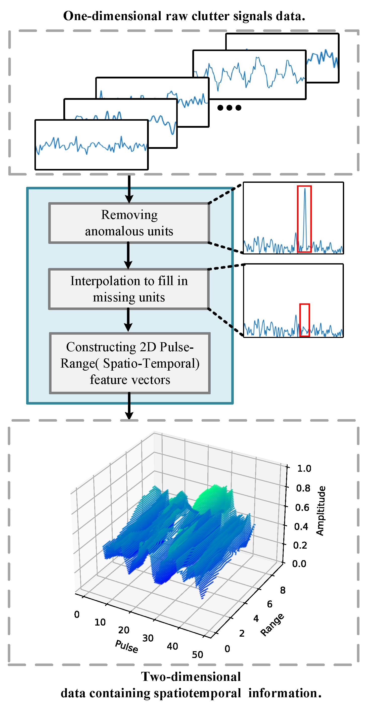
  • Construction of spatiotemporal feature vectors: Multiple time-domain signals are layered within a single range unit because the sea clutter data are divided into range cells according to the correlation length of the sea clutter. A two-dimensional vector representation of sea clutter is created via this partitioning procedure, which aids in the retention of the spatiotemporal properties of the sea clutter data. Figure 3 shows the procedure for creating the spatiotemporal feature vectors.
  • Data preprocessing and spatiotemporal feature construction: To obtain a pure sea clutter dataset while preserving its intrinsic spatiotemporal structure, let the raw complex echoes be X C M × P (with M range cells and P pulses). We construct a three-channel real tensor by
    A R M × P × 3 , A m , p , : = Re X m , p , Im X m , p , arg X m , p
    Outlier removal. Small targets or sea spikes—whose amplitudes deviate sharply from neighbors—are marked by index intervals S = { ( s k , e k ) } k = 1 K . For each ( s k , e k ) , we set
    A m , p , c NaN , m = s k , , e k , p , c ,
    thus excising anomalous units from the dataset.
    Interpolation. To restore continuity, missing values are filled using three complementary schemes: linear interpolation, mean interpolation, and polynomial interpolation along the range (spatial) dimension, which can preserve statistical diversity and avoid bias towards any single filling strategy.
    Global window determination. For each sample, we estimate the time domain autocorrelation length (in pulses) and select a window length that matches the scale, ensuring that each window spans at least one estimated correlation length, thereby preserving the coherence between pulses within the sample; at the same time, all samples are anchored to a common minimum correlation scale to obtain more comparable cross-sample statistics.
    Spatiotemporal feature extraction. During iteration, a random file is loaded and a sub-tensor of shape R d × w × 3 is extracted:
    X t , p , c = A ^ m + t , i + p , c , m U { 0 , , M d } , i U { 0 , , P w } ,
    where t = 0 , , d 1 (range offset) and p = 0 , , w 1 (pulse offset). This block preserves temporal correlation over w pulses and spatial correlation over d range cells, yielding a spatiotemporal patch (tensor) for downstream learning.

3.2. Transformer GAN Model Architecture

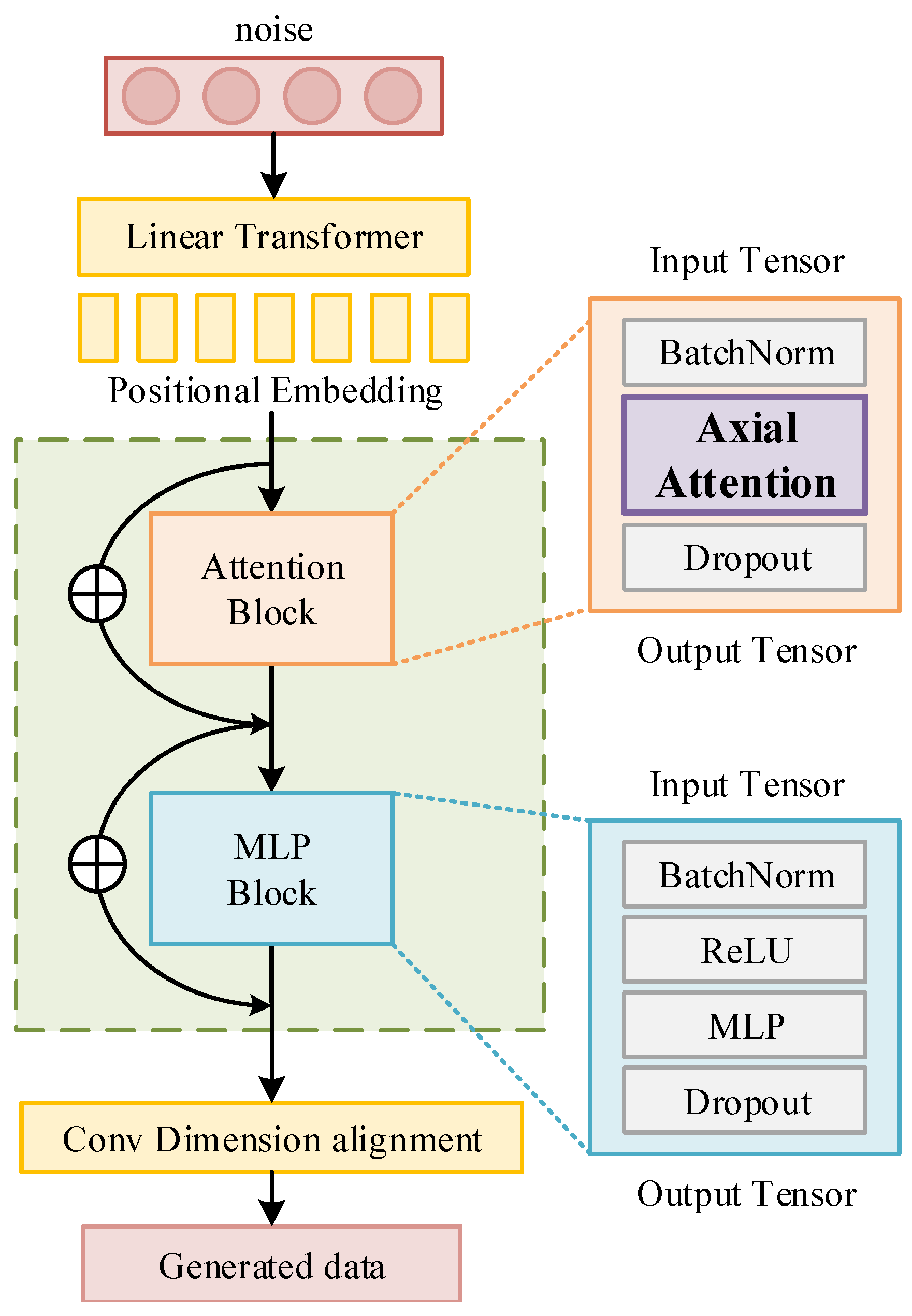
Overall architecture: In this work, the discriminator and generator of the generative adversarial network (GAN) are built on the basis of the transformer encoder. Two composite blocks make up the encoder. The attention module, which is the initial block, records internal correlations within the input sequence. The multihead attention mechanism is highly effective in modeling long-range dependencies. The standard attention mechanism, on the other hand, necessitates calculating the dot product of each pair of elements in the input tensor, which is computationally costly for the variable-length feature vectors created in this paper. The computational complexity for each position is O(P × R), where P is the number of pulses, and R is the number of range cells. To reduce the complexity, the proposed model employs axial attention as a replacement for the traditional multihead attention mechanism, and the specific design is described in Section 3.2.
  • Normalization, activation, and regularization: Each block adopts a GELU nonlinearity followed by a feedforward MLP, with residual connections between blocks to preserve information and stabilize gradient flow. To mitigate covariate shift, we use a pre-normalization strategy: grid-based branches processed by convolutions use BN, whereas transformer sublayers use LayerNorm [50]. Dropout is applied after the main transforms to reduce overfitting. The combination of BN, LN, GELU, MLP, and the dropout configuration yields stable optimization for sea clutter generation and maintains generalization across sea states [51,52,53].
    The architecture of the generator is illustrated in Figure 4. Before receiving real data, the generator first receives the input of the noise. To assist the model in understanding the spatiotemporal correlations present in the data, the noise sequence is then split into several patches, each of which is then enhanced with position encoding. These patches are then sent into the encoder’s blocks for additional processing. The generator can efficiently capture the spatiotemporal properties of the data and produce high-quality samples by segmenting the noise sequence into patches and incorporating position encoding.
    The discriminator uses the Vision Transformer (ViT) technique, which classifies input data into actual data and creates categories via an encoder [54]. Owing to the special nature of clutter signals and the characteristics of neural networks, real data need to be converted into real numbers and normalized before being fed into the discriminator. Given a certain spatiotemporal vector X = x 1 , x 2 , x R obtained from the processing in Section 3.1, where x i M P , P is the number of pulses, and R is the number of range cells. To retain the information of the real signal data, we transformed the real and imaginary parts into dual channels, i.e., x i M P × C , where C is the number of channels. Owing to the large range of signal amplitudes, which can lead to difficulties or even failure in model convergence, it is necessary to normalize the real data. ViT consistently divides an image into numerous blocks of the same width and height. Similarly, in this paper, we take a similar strategy by evenly partitioning the sea clutter data into numerous multidimensional segments by using the time step as the width and the correlation length of the sea clutter as the height of the image. Each segment also includes location encoding to help the discriminator better grasp the spatial and temporal characteristics of the clutter.
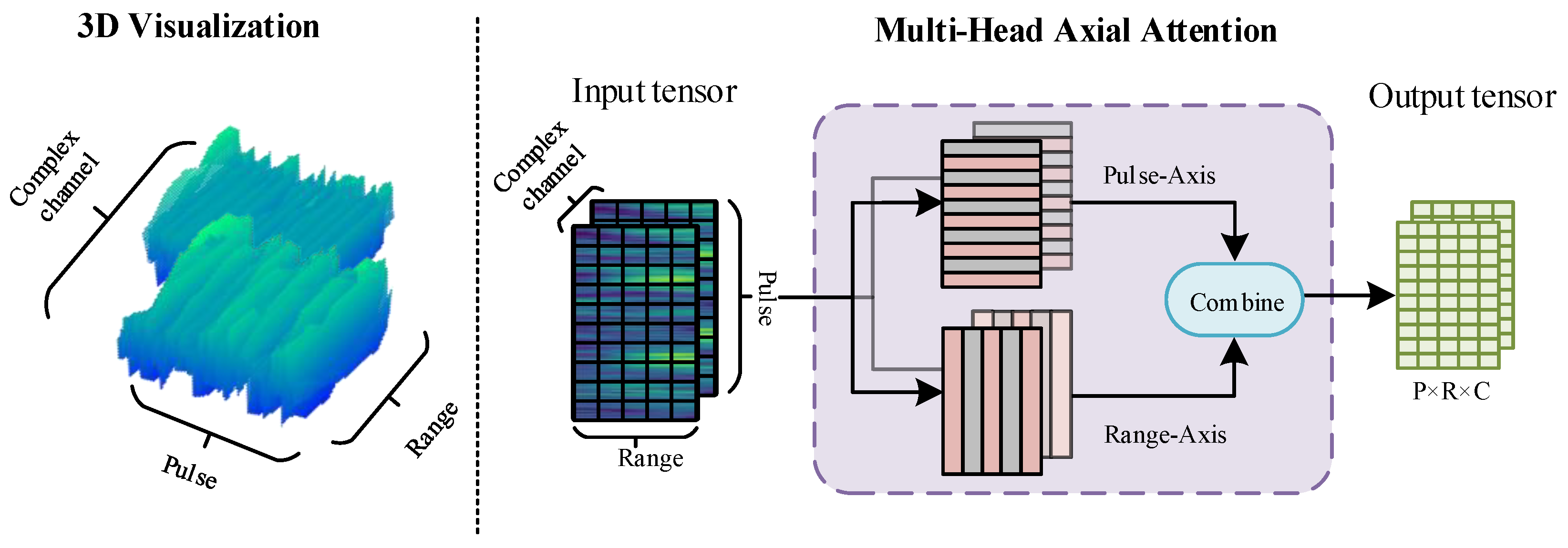
  • Pulse-range axial attention: Sea clutter data display variations in properties across various dimensions, unlike flat images. The correlations in clutter data between various units in various dimensions are different from those between various pixels in a 2D flat image. We breakdown the multihead attention mechanism into two modules to allow the network to learn the correlations between various dimensions and units separately and overcome the difficulty of computing global attention. The first module performs self-attention in the pulse dimension, whereas the second module conducts self-attention in the spatial dimension. This operation is referred to as pulse-range axial attention. By employing axial attention, we efficiently capture relevant information in both dimensions while mitigating the computational complexity burden associated with computing global attention. By adopting axial attention, it efficiently captures the relevant information in both dimensions, avoiding the burden of computing global attention while maintaining the ability to learn correlations in the data effectively. This approach allows the network to focus on important relationships within each dimension and improves the model’s ability to process sea clutter data effectively.
    Applying axial attention to both the pulse and spatial dimensions effectively simulates the original attention mechanism and significantly improves computational efficiency. Figure 5 illustrates the implementation of the axial attention designed in this paper, which is a parallelized spatiotemporal axial attention mechanism. In terms of computation, attention is performed independently along both dimensions, reducing the required computational complexity per position in the spatiotemporal vector from O ( P × R ) to O ( P + R ) . Furthermore, the feature vectors after the attention operation still preserve global information and do not alter the size of the input tensor. For a specific position ( i , j ) , the output of axial attention y i , j is computed as follows:
    y i , j 1 = s o f t m a x ( q i , j K 1 T d ) V 1 y i , j 2 = s o f t m a x ( q i , j K 2 T d ) V 2 y i , j = y i , j 1 + y i , j 2 .
    Here, q i , j represents the query vector corresponding to position ( i , j ) , while K 1 and V 1 are the key and value matrices along the pulse dimension, respectively. Similarly, K 2 and V 2 are the key and value matrices along the spatial unit dimension. To enable the network to learn the characteristics of different dimensions separately, the parameters of the two modules are not shared. This axial attention design allows the network to independently learn and capture important feature information in the pulse and spatial dimensions with some degree of discrimination. As a result, it better models sea clutter data in different dimensions.
  • Axial attention efficiency analysis in sea clutter generation: In two-dimensional sea clutter generation, standard Multi-Head Self-Attention (MHSA) computes attention over the entire sequence of length N = H × W at once, incurring both time and memory complexity
    O ( N 2 d ) = O ( H 2 W 2 d ) ,
    where H and W are the token counts along temporal and spatial dimensions, and d is the embedding dimension. For large windows, this quadratic growth becomes prohibitive.
    Axial attention splits the 2D attention into two 1D attentions: row-wise (length W) and column-wise (length H). Its combined complexity is
    O ( H W 2 d ) row - attention + O ( W H 2 d ) column - attention = O H W ( H + W ) d ,
    and the memory for attention weights reduces to
    O ( H W 2 + H 2 W ) = O H W ( H + W ) ,
    instead of O ( H 2 W 2 ) .
    When H = W = N , MHSA has complexity O ( N 2 ) , whereas axial attention is
    O N N = O ( N 1.5 ) .
    In summary, compared to standard Multi-Head Self-Attention (MHSA) in sea clutter generation, axial attention delivers substantial efficiency improvements; it reduces computational and memory complexity from O ( N 2 ) to O ( N 1.5 ) while maintaining identical parameter counts. For typical operational window sizes ( N 256 t o 16,384), axial attention achieves order-of-magnitude speed-ups (10-fold) and drastically reduces storage requirements for attention maps.
  • Training procedure:
    L a d v = E x D a d v ( x ) E z , c D a d v ( G ( z , c ) ) λ g p E x ^ x ^ D a d v ( x ^ ) 2 1 2
    The loss of the generator is
    G l o s s = E z , c D a d v ( G ( z , c ) )
    The loss of the discriminator is
    D l o s s = D f a k e + D r e a l + λ g p E x ^ ( x ^ D a d v ( x ^ ) 2 1 ] 2
    Overall, the generator aims to minimize the loss as much as possible to confuse real and generated sea clutter data; the discriminator aims to maximize the loss to distinguish between real and generated data. The loss function for the generator includes a penalty term with a weight λ to enforce a gradient penalty. x ^ represents a linearly sampled sample from both real sea clutter data and generated sea clutter data. Adding the penalty term helps to distribute the gradient descent weights more evenly. In this experiment, λ is set to 10.
    The Adam optimizer is chosen for optimization, with a learning rate of 0.0001 for the generator and 0.003 for the discriminator. β 1 = 0.9 and β 2 = 0.999 . Additionally, a weight decay of 0.01 is applied. Both the generator and discriminator have a batch size of 64.
    To balance the differences between the generator and discriminator, a training strategy is employed. The discriminator is trained for five iterations first. After that, both generators and the discriminators are alternately trained for three iterations in each cycle. This process is repeated to ensure the balanced training of the generator and discriminator in the model.

4. Experiments

4.1. Training Setup and Resource Consumption

Hardware. The hardware configuration is a workstation equipped with four NVIDIA RTX 4090 GPUs (24 GB memory per card), a 16-core CPU, 64 GB system memory, a 30 GB system disk, and a 100 GB dedicated data disk.
Memory footprint. The peak GPU memory usage of the standard multi-head attention mechanism is about 40 GB; after adopting the axial attention mechanism, the memory requirement is reduced to about 25 GB (a relative reduction of 37%).
Baseline: This work employs Diffusion [55], Auto-Regressive (AR) [56], and WaveGAN [18] as the baseline to show the efficacy of the proposed method (Ours).
The Diffusion model employed in this work follows the denoising paradigm, where a sequence of small-step Gaussian noise injections and iterative denoising network recoveries establishes a mapping between the data distribution and a noise distribution. In the forward diffusion stage, clean radar clutter samples are gradually corrupted by Gaussian noise with variance β t , as described by
q ( x t x t 1 ) = N x t ; 1 β t x t 1 , β t I ,
and in the reverse denoising stage, a trained denoising network μ θ based on transformer restores the signal from noise:
p θ ( x t 1 x t ) = N x t 1 ; μ θ ( x t , t ) , σ t 2 I .
The traditional Auto-Regressive (AR) model predicts each sample as a linear combination of the previous p samples:
x n = k = 1 p a k x n k + ε n ,
where we set the model order to p = 10 and estimate the coefficient vector { a k } via Least Squares on the training data, with ε n denoting white noise residual.
An intuitive evaluation of the generated radar clutter quality is difficult due to its distinct time-frequency characteristics compared to visual or auditory signals. We first performed qualitative assessments by visually comparing the time-domain waveforms and frequency spectra of real and generated clutter, conducting PCA-based dimensionality reduction to observe clustering in 2D/3D feature space, and fitting amplitude distributions, such as Rayleigh or Gaussian mixtures, to examine consistency with real data. Quantitatively, we computed the cosine similarity and Euclidean distance between the statistical feature vectors (e.g., autocorrelation and power spectral density) of the generated and real clutter, fitted Gaussian models to the spectral power distribution to compare mean and variance parameters, and evaluated amplitude distribution agreement using metrics like Wasserstein distance or Kullback–Leibler divergence. Finally, we compared our proposed method with the state-of-the-art WaveGAN [18] and Diffusion Model [55] in the clutter generation task.

4.2. Result and Analysis

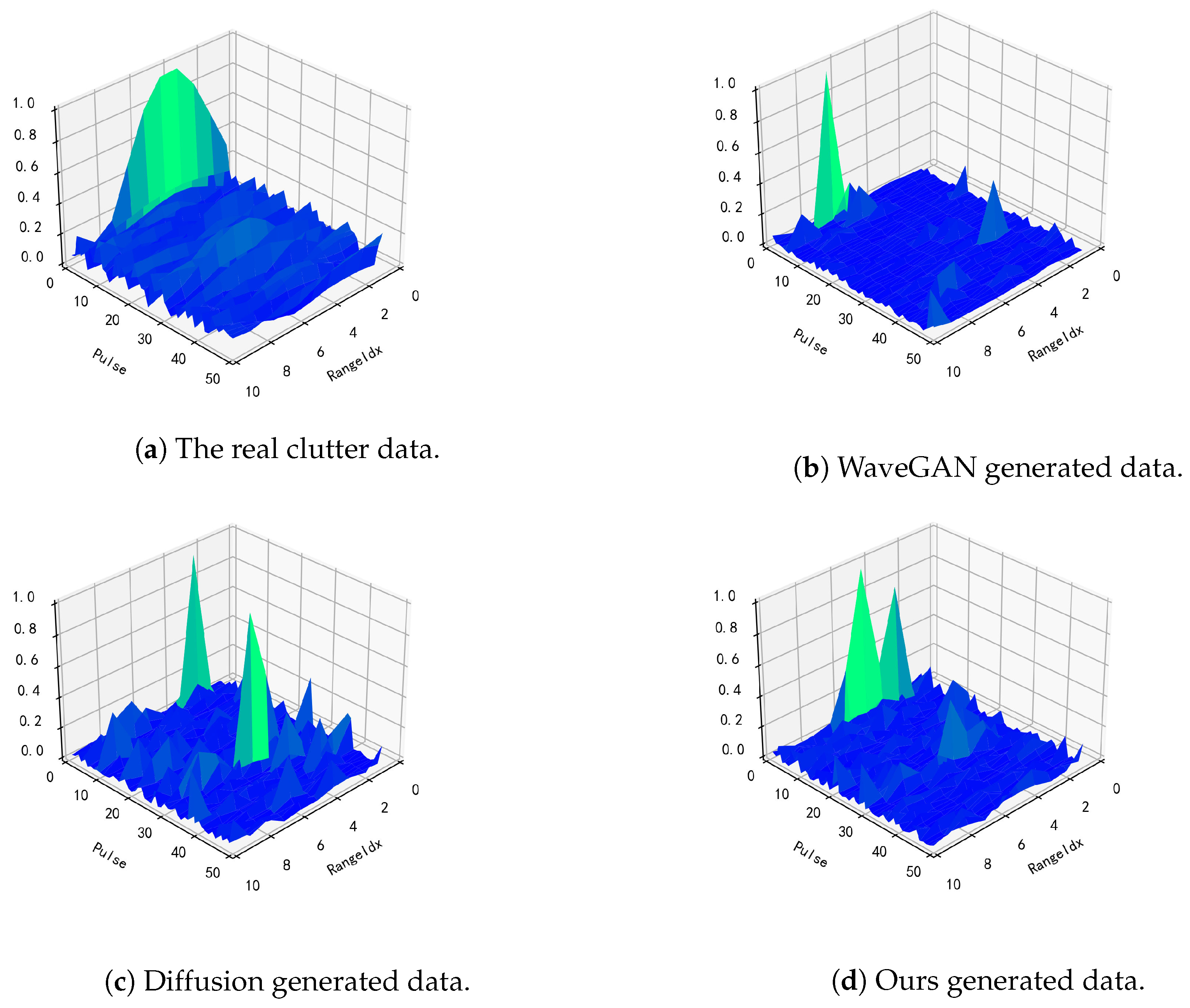
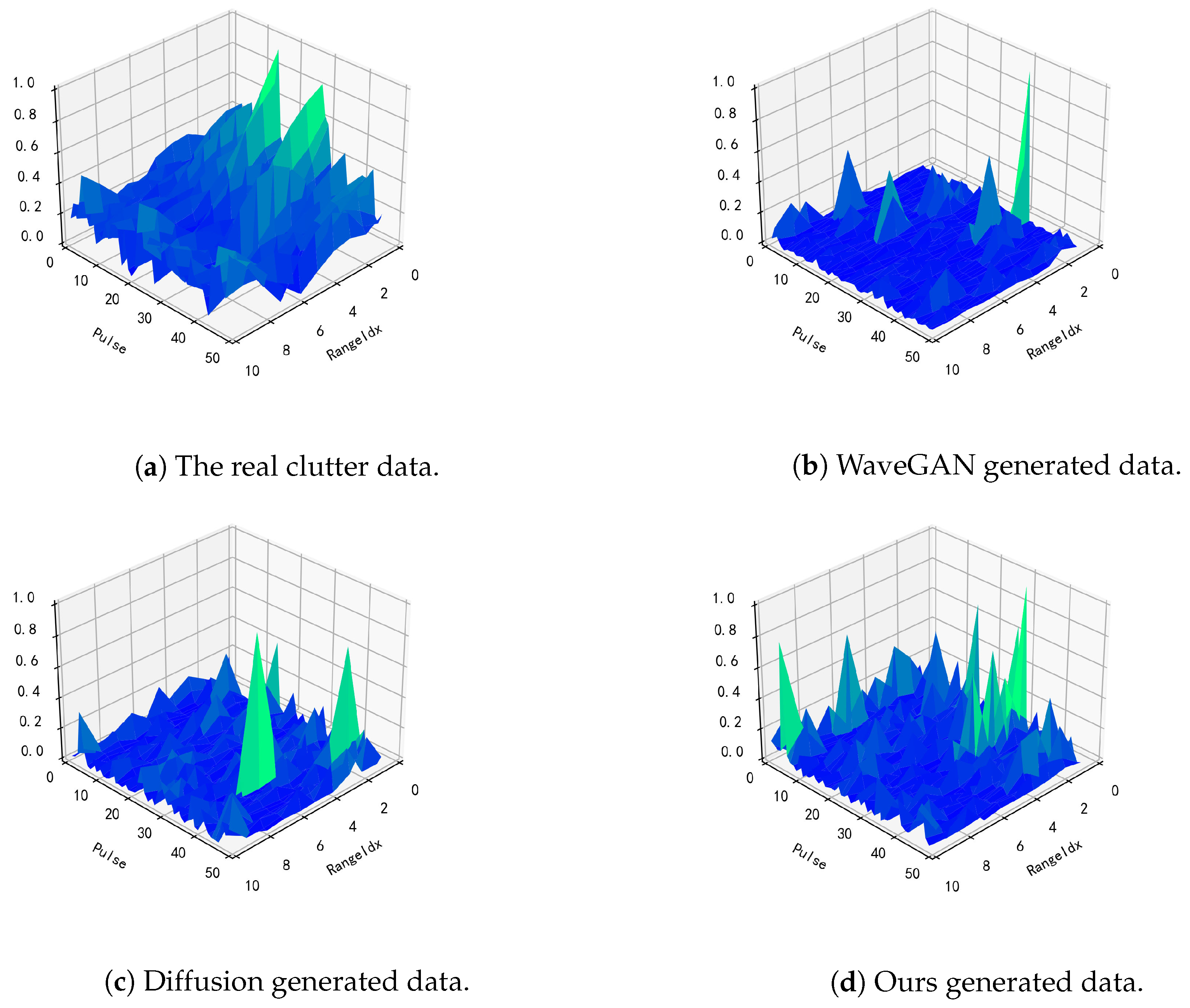
Amplitude visual comparison: Compared to the low sea state in Figure 6, the high sea state in Figure 7 exhibits a fragmented background with localized peaks and pulse bursts, indicating short temporal coherence and anisotropic coupling consistent with breaking waves and multiscale swells. The baseline behavior is similar across sea states: WaveGAN tends to exhibit isolated spikes against a reduced background due to insufficient constraints on cross-pulse and range statistics from locally focused adversarial learning. The diffusion model produces a more continuous background but retains energy compression and residual spikes, reflecting the denoising scheme’s poor matching of the enhanced receptive field with anisotropic clutter and MSE-biased reconstruction. In contrast, our method maintains background continuity in calm conditions while allowing for necessary undulations and fat-tailed behavior without disrupting spatiotemporal consistency in complex conditions. Echoes appear as coherent clusters, and the background maintains appropriate roughness and transitions. Overall, our method balances energy compression, background smoothness, and coherence, exhibiting adaptability across sea states and good agreement with measurements.
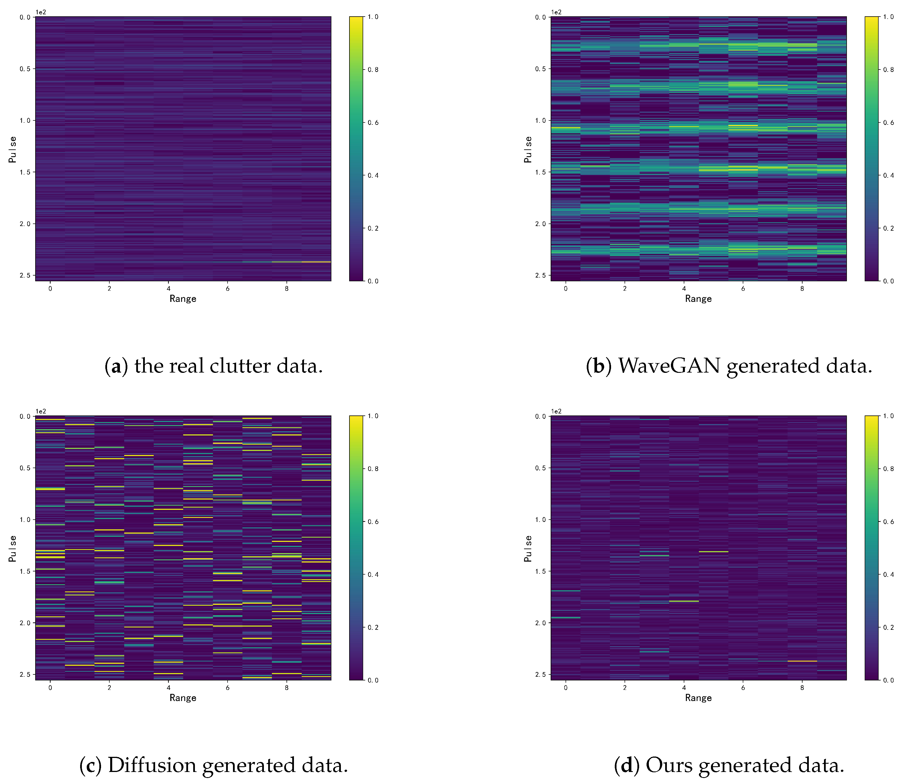
Two-dimensional heatmaps: As Figure 8 shows, in the high sea state, the measurement presents a raised clutter floor with clustered local enhancements; WaveGAN tends to produce few extreme highs over a sparse background, and Diffusion yields over-compacted energy with an over-smoothed background, whereas Ours raises the background level while preserving realistic roughness and clustered enhancements, maintaining spatiotemporal consistency with the real echoes. The qualitative evolution of generation quality follows the same pattern under both low and high sea states.
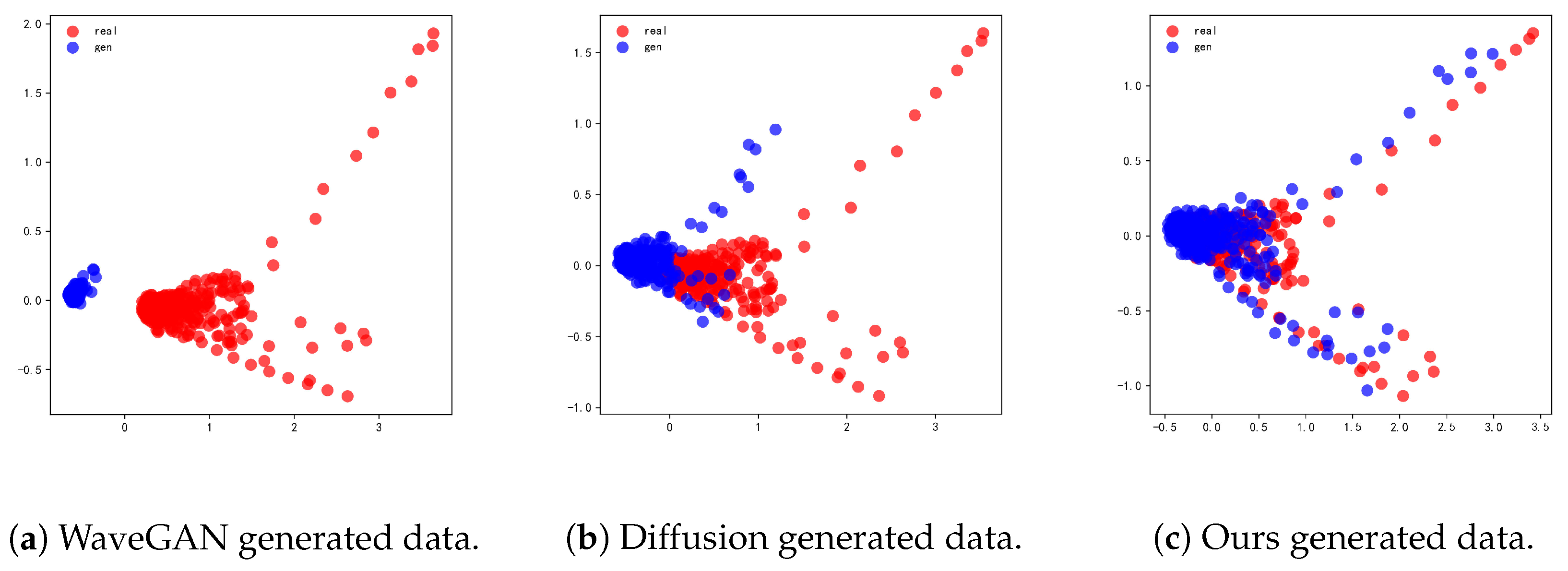
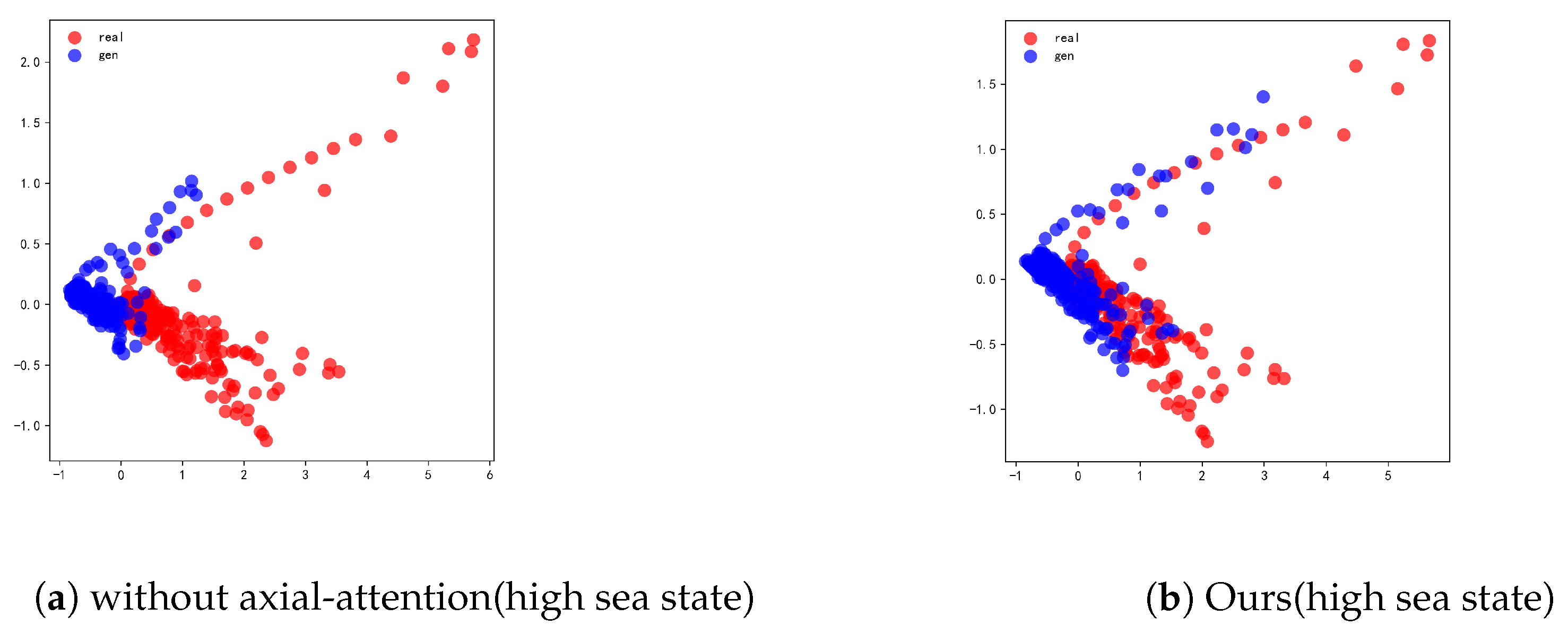
Visualizations with PCA: We applied principal component analysis (PCA) to project the two datasets onto a two-dimensional plane for visual comparison, highlighting the coverage of the generated data relative to the real data [57]. As shown in Figure 9, under high sea states, the real distribution becomes a stretched curved manifold; WaveGAN shrinks to a narrow chain, Diffusion expands but still has rotations and misalignments, and it cannot fully represent the ends and inflection points, while our method follows the real trajectory, covers the core and main tail, and does not violate spatiotemporal consistency. At the same time, the qualitative patterns of the generation quality of our method and the comparison methods are the same under low and high sea states. In terms of comprehensive fidelity indicators, our method significantly outperforms Diffusion and WaveGAN models, which is due to the local adversarial bias of WaveGAN, the scheduling and receptive field mismatch of Diffusion, and our joint spatiotemporal modeling with implicit spectral correlation tightening constraints.
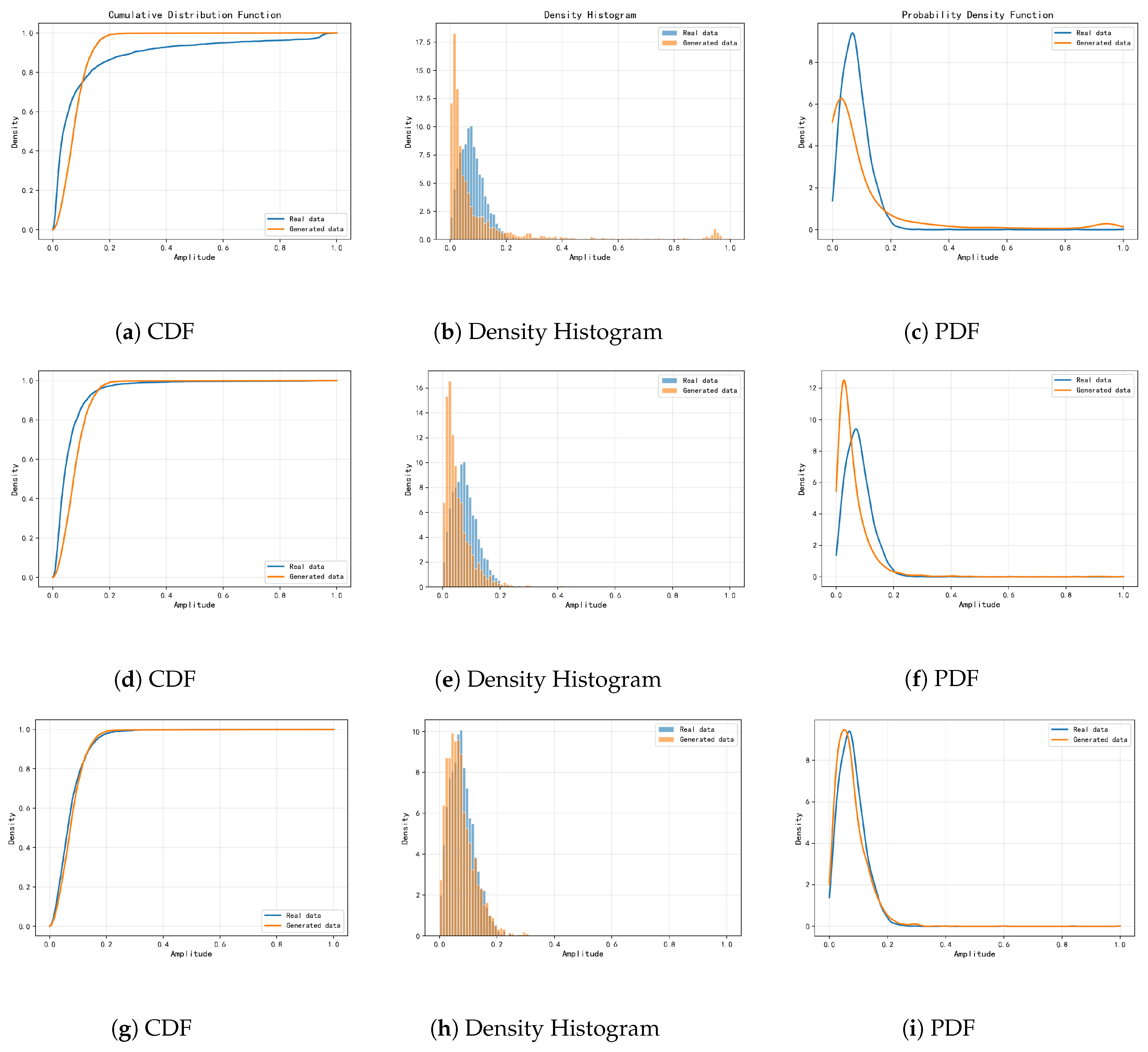
Amplitude–distribution analysis: Figure 10 compares the cumulative distribution functions (CDFs), empirical histograms, and kernel–density PDFs between generated and real amplitudes across epochs ( epoch = 100 / 1000 / 3660 ). For the high sea state, at epoch = 100 , the generated CDF is left-shifted at small amplitudes, the histogram mode is narrower and left-shifted, and the PDF is lower on the right; by epoch = 1000 , the distribution body is better aligned, although the tail shape still differs; by epoch = 3660 , the CDFs coincide over 0–0.3, and the histogram bodies overlap, with a residual gap in the right tail of the PDF. The same evolution in generation quality—early low-amplitude shrinkage followed by body alignment with a slower improvement in the tail—holds across sea states, indicating a consistent convergence trend under both low and high conditions.
To evaluate the accuracy and objectivity of the experimental results, we conducted mean squared error (MSE) and Kolmogorov–Smirnov (K-S) tests on the PDF and CDF distributions. The experimental results presented in Table 2 indicate that, in comparison with WaveGAN, the clutter signals generated by our method more closely resemble real data in terms of amplitude distribution.
Effects of axial attention on resource consumption and clutter modeling: As Table 2, Table 3 and Table 4 and Figure 11 and Figure 12 show, decomposing 2D self-attention along the pulse and range axes reduces the theoretical cost from standard MHSA O ( N 2 ) with N = P R to O ( P N + R N ) ; Table 3 indicates concurrent reductions in training time, memory footprint, and inference latency. We further analyzed training resource and runtime requirements, showing that axial attention reduces per-epoch training time roughly from 5979 to 4325 and peak GPU memory roughly from 23.79 GB to 16.9 GB (for P = 200 4096 , R = 10 150 ). In Figure 11, for the low sea state, the model without axial attention tends to produce discrete bright patches and blocky textures with weaker cross-axis correlation, whereas with axial attention, the background level and streak orientation align better with the measurement. For the high sea state, the measurement exhibits a raised background with clustered enhancements; without axial attention, the result shows stronger smoothing and weaker clustering, while axial attention restores clustered enhancements and texture anisotropy closer to the real data. The PSD-parameter errors in Table 2 are consistent; with axial attention, the alignment of location and spread ( μ , σ ) improves, while the match of the shape parameter a reflects a modest tradeoff. Overall, axial attention lowers resource usage while strengthening long-range dependencies along both axes, yielding textures and several spectral statistics that are closer to the measurements across sea states.
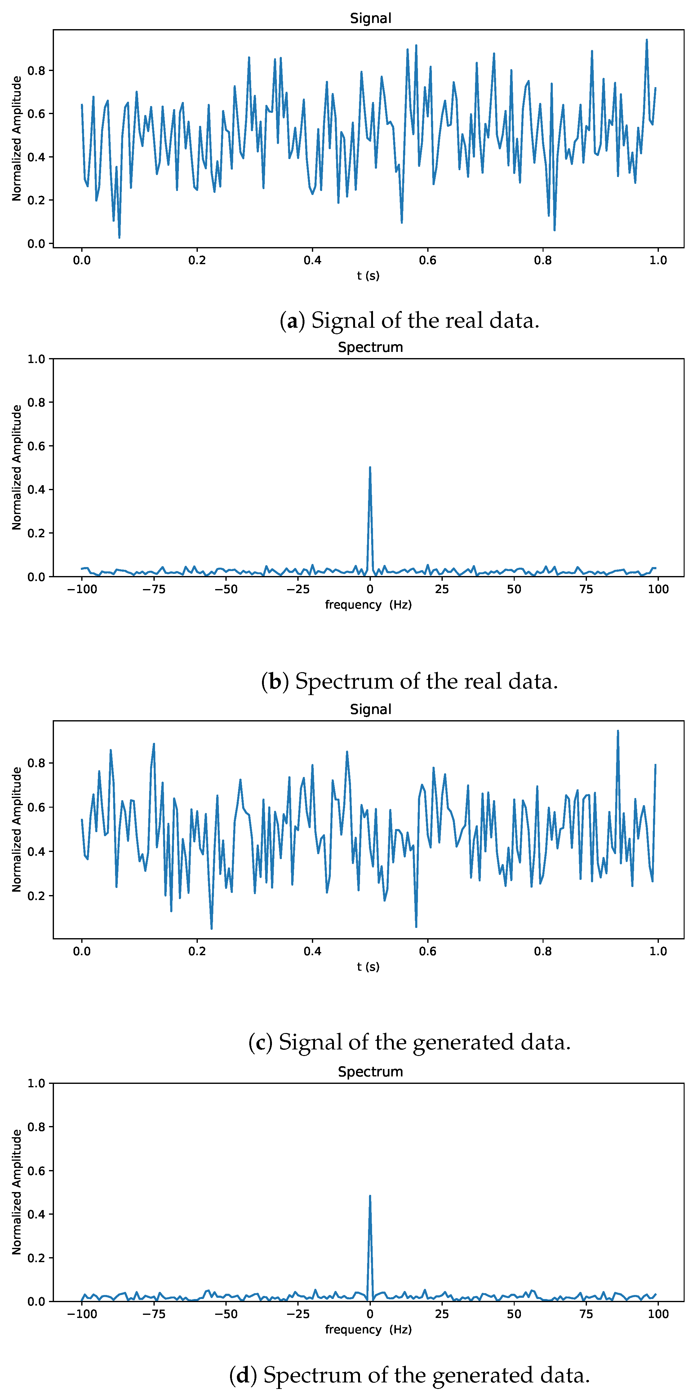
Doppler characteristics: Figure 13 depicts the zero-frequency bilateral spectra of both the generated and real data after undergoing Fourier transformation. It can be observed that the spectra of the generated data and real data are similar.
Additionally, we modeled the average Doppler shape of the generated and real data using a Gaussian distribution. The Gaussian model is as follows:
S ( f ) = a × e x p [ ( f μ ) 2 2 σ f 2 ]
Here, a is the shape parameter, and μ and σ are scale parameters. These parameters can characterize different Gaussian distributions. If the shape and scale parameters are close, it indicates a similarity between the generated data and real data in terms of power spectral density. Conversely, dissimilarity suggests a significant difference between the generated data and real data. We employ absolute error to compare the parameter differences between real data and generated data from different models. Table 5 and Table 6 shows the errors in scale parameters for different models. The model proposed in this paper exhibits superior performance in terms of the scale parameter.
Similarity scores: This work uses cosine similarity (Cos-Sim) and Jensen–Shannon distance (Js-Dis) to measure the similarity between generated and real data. Initially, we extracted eight representative statistical features (mean, median, mode, quartiles, standard deviation, covariance, minimum, and maximum) from each batch of data, forming a one-dimensional feature vector. Cosine similarity measures the average cosine similarity between all real signals and the corresponding synthetic signals. Values close to 1 indicate greater similarity between the two feature vectors. The Jensen–Shannon distance is a method for measuring the similarity between two class probability distributions. We treated each extracted feature as an array of values following a normal distribution and computed the Jensen–Shannon distance for each corresponding feature between the real and synthetic feature vectors.
The experimental results in Table 7 and Table 8 indicate that our model results in higher cosine similarity and a lower Jensen–Shannon distance for the generated data, outperforming WaveGAN overall. The ablation experiments also show that axial attention improves the quality of generated data by capturing the spatiotemporal joint characteristics of sea clutter.

5. Conclusions

In this work, we have presented a novel transformer-driven GAN framework for high-fidelity sea clutter generation, in which (i) two-dimensional spatio-temporal feature maps are directly modeled; (ii) standard multi-head attention is replaced by a pulse–range bidirectional axial attention mechanism to capture long-range dependencies along both pulse and range dimensions; and (iii) BatchNorm, LayerNorm, and moderate Dropout are employed layer-wise to ensure stable and generalizable training under the non-stationary conditions of real radar returns. Extensive experiments on X-band IPIX datasets demonstrate that our method achieves superior modeling accuracy—quantified by lower parameter errors and higher similarity scores—and generates clutter samples whose PCA and statistical amplitude distributions closely match real clutter.
Future directions: Future work will focus on several key directions: firstly, conducting systematic module-level ablation studies (e.g., positional encoding and residual connections) to quantify their impact beyond preliminary analysis; to this end, the scope of methodological references will be expanded by integrating insights from radar signal processing frameworks [29,30] and advanced deep learning models [31,33]. Secondly, implementing and benchmarking the complete pipeline on edge GPUs to evaluate end-to-end latency and integration with commercial radar interfaces. Furthermore, enhancing ethical safeguards is crucial, requiring the development of adversarial robustness tests and differential privacy protocols to prevent malicious use of generated clutter echoes in electronic warfare. Finally, exploring multimodal clutter generation by incorporating polarimetric channels and leveraging diffusion-based generative models [58] to achieve richer spectral-temporal diversity.

Author Contributions

X.Z.: Conceptualization, methodology, data curation, and writing—original draft preparation; J.R.: Validation, and writing—review; W.T.: Data analysis; A.C.: software development; X.L.: Formal analysis; C.W.: Editing and visualization; C.J.: Conceptualization and methodology; M.Z.: Methodology refinement and visualization support; X.X.: Validation. All authors have read and agreed to the published version of the manuscript.

Funding

This research was funded by the National Natural Science Foundation of China under Grant 62201434 and the Fundamental Research Funds for the Central Universities No.30923010933.

Data Availability Statement

The original contributions presented in this study are included in the article. Further inquiries can be directed to the corresponding authors.

Conflicts of Interest

Author Xueyong Xu was employed by the company North Information Control Reasearch Academy Group Company Limited. The remaining authors declare that the research was conducted in the absence of any commercial or financial relationships that could be construed as a potential conflict of interest.

Correction Statement

This article has been republished with a minor change. The change does not affect the scientific content of the article and further details are available within the backmatter of the website version of this article.

References

  1. Ward, K.D.; Tough, R.J.; Watts, S. Sea clutter: Scattering, the k distribution and radar performance. Waves Random Complex Media 2007, 17, 233–234. [Google Scholar] [CrossRef]
  2. Kim, J.; Kim, T.; Ryu, J.-G.; Kim, J. Spatiotemporal graph neural network for multivariate multi-step ahead time-series forecasting of sea temperature. Eng. Appl. Artif. Intell. 2023, 126, 106854. [Google Scholar] [CrossRef]
  3. Fernández, J.R.M.; de la Concepción Bacallao Vidal, J. Fast selection of the sea clutter preferential distribution with neural networks. Eng. Appl. Artif. Intell. 2018, 70, 123–129. [Google Scholar] [CrossRef]
  4. Pérez-Fontán, F.; Vazquez-Castro, M.A.; Buonomo, S.; Poiares-Baptista, J.P.; Arbesser-Rastburg, B. S-band lms propagation channel behaviour for different environments, degrees of shadowing and elevation angles. IEEE Trans. Broadcast. 1998, 44, 40–76. [Google Scholar] [CrossRef]
  5. Jie, Z.; Dong, C.; Dewei, S. K distribution sea clutter modeling and simulation based on zmnl. In Proceedings of the 2015 8th International Conference on Intelligent Computation Technology and Automation (ICICTA), Nanchang, China, 14–15 June 2015; pp. 506–509. [Google Scholar]
  6. Yi, L.; Yan, L.; Han, N. Simulation of inverse gaussian compound gaussian distribution sea clutter based on sirp. In Proceedings of the 2014 IEEE Workshop on Advanced Research and Technology in Industry Applications (WARTIA), Ottawa, ON, Canada, 29–30 September 2014; pp. 1026–1029. [Google Scholar]
  7. Ye, L.; Xia, D.; Guo, W. Comparison and analysis of radar sea clutter k distribution sequence model simulation based on zmnl and sirp. Model. Simul. 2018, 7, 8–13. [Google Scholar] [CrossRef]
  8. Guo, S.; Zhang, Q.; Shao, Y.; Chen, W. Sea clutter and target detection with deep neural networks. In Proceedings of the 2nd International Conference on Artificial Intelligence and Engineering Applications, Guilin, China, 23–24 September 2017; pp. 316–326. [Google Scholar]
  9. Baek, M.-S.; Kwak, S.; Jung, J.-Y.; Kim, H.M.; Choi, D.-J. Implementation methodologies of deep learning-based signal detection for conventional mimo transmitters. IEEE Trans. Broadcast. 2019, 65, 636–642. [Google Scholar] [CrossRef]
  10. Goodfellow, I.; Pouget-Abadie, J.; Mirza, M.; Xu, B.; Warde-Farley, D.; Ozair, S.; Courville, A.; Bengio, Y. Generative adversarial nets. In Advances in Neural Information Processing Systems; Curran Associates Inc.: Red Hook, NY, USA, 2014; Volume 27. [Google Scholar]
  11. Balouji, E.; Salor, Ö.; McKelvey, T. Deep learning based predictive compensation of flicker, voltage dips, harmonics and interharmonics in electric arc furnaces. IEEE Trans. Ind. Appl. 2022, 58, 4214–4224. [Google Scholar] [CrossRef]
  12. Guo, S.; Zhou, B.; Yang, Y.; Wu, Q.; Xiang, Y.; He, Y. Multi-source ensemble learning with acoustic spectrum analysis for fault perception of direct-buried transformer substations. IEEE Trans. Ind. Appl. 2022, 59, 2340–2351. [Google Scholar] [CrossRef]
  13. Yamamoto, R.; Song, E.; Kim, J.-M. Parallel wavegan: A fast waveform generation model based on generative adversarial networks with multi-resolution spectrogram. In Proceedings of the ICASSP 2020—2020 IEEE International Conference on Acoustics, Speech and Signal Processing (ICASSP), Barcelona, Spain, 4–8 May 2020; pp. 6199–6203. [Google Scholar]
  14. Yoon, J.; Jarrett, D.; Van der Schaar, M. Time-series generative adversarial networks. In Advances in Neural Information Processing Systems; Curran Associates Inc.: Red Hook, NY, USA, 2019; Volume 32. [Google Scholar]
  15. Jing, J.; Li, Q.; Ding, X.; Sun, N.; Tang, R.; Cai, Y. Aenn: A generative adversarial neural network for weather radar echo extrapolation. Int. Arch. Photogramm. Remote Sens. Spat. Inf. Sci. 2019, 42, 89–94. [Google Scholar] [CrossRef]
  16. Saarinen, V.; Koivunen, V. Radar waveform synthesis using generative adversarial networks. In Proceedings of the 2020 IEEE Radar Conference (RadarConf20), Florence, Italy, 21–25 September 2020; pp. 1–6. [Google Scholar]
  17. Truong, T.; Yanushkevich, S. Generative adversarial network for radar signal synthesis. In Proceedings of the 2019 International Joint Conference on Neural Networks (IJCNN), Budapest, Hungary, 14–19 July 2019; pp. 1–7. [Google Scholar]
  18. Ma, X.; Zhang, W.; Shi, Z.; Zhao, X. Clutter simulation based on wavegan. In Proceedings of the International Conference on Radar Systems, Edinburgh, UK, 24–27 October 2022; pp. 605–611. [Google Scholar]
  19. Donahue, C.; McAuley, J.; Puckette, M. Adversarial audio synthesis. In Proceedings of the International Conference on Learning Representations, Vancouver, BC, Canada, 30 April–3 May 2018. [Google Scholar]
  20. Chen, H.; Chen, F.; He, H. A sea–land clutter classification framework for over-the-horizon radar based on weighted loss semi-supervised generative adversarial network. Eng. Appl. Artif. Intell. 2024, 133, 108526. [Google Scholar]
  21. Guo, M.-F.; Liu, W.-L.; Gao, J.-H.; Chen, D.-Y. A data-enhanced high impedance fault detection method under imbalanced sample scenarios in distribution networks. IEEE Trans. Ind. Appl. 2023, 59, 4720–4733. [Google Scholar] [CrossRef]
  22. Thomas, J.A.; Cover, T.M. Elements of Information Theory; Tsinghua University Press: Beijing, China, 2006. [Google Scholar]
  23. Smirnoff, N.W. On the estimation of the discrepancy between empirical curves of distribution for two independent samples. Bull. MathéMatique L’Université Mosc. 1939, 2, 3–11. [Google Scholar]
  24. Walker, D. Doppler modelling of radar sea clutter. IEE Proc.-Radar Sonar Navig. 2001, 148, 73–80. [Google Scholar] [CrossRef]
  25. Angelliaume, S.; Rosenberg, L.; Ritchie, M. Modeling the amplitude distribution of radar sea clutter. Remote Sens. Target Detect. Mar. Environ. 2019, 11, 319. [Google Scholar] [CrossRef]
  26. Vondra, B.; Bonefacic, D. Mitigation of the Effects of Unknown Sea Clutter Statistics by Using Radial Basis Function Network. Radioengineering 2020, 29, 215–227. [Google Scholar] [CrossRef]
  27. Wen, B.; Wei, Y.; Lu, Z. Sea clutter suppression and target detection algorithm of marine radar image sequence based on spatio-temporal domain joint filtering Entropy. Signal Data Anal. 2022, 24, 250. [Google Scholar]
  28. Chen, T.; Kornblith, S.; Norouzi, M.; Hinton, G. A simple framework for contrastive learning of visual representations. In Proceedings of the International Conference on Machine Learning, Online, 13–18 July 2020; pp. 1597–1607. [Google Scholar]
  29. Skolnik, M.I. Radar handbook. IEEE Aerosp. Electron. Syst. Mag. 2008, 23, 41. [Google Scholar] [CrossRef]
  30. Greco, M.S.; Gini, F. Statistical analysis of high-resolution SAR ground clutter data. IEEE Trans. Geosci. Remote Sens. 2007, 45, 566–575. [Google Scholar] [CrossRef]
  31. Smith, G.E.; Woodbridge, K.; Baker, C.J. Radar micro-Doppler signature classification using dynamic time warping. IEEE Trans. Aerosp. Electron. Syst. 2010, 46, 1078–1096. [Google Scholar] [CrossRef]
  32. Li, G.; Song, Z.; Fu, Q. A convolutional neural network based approach to sea clutter suppression for small boat detection. Front. Inf. Technol. Electron. Eng. 2020, 21, 1504–1520. [Google Scholar] [CrossRef]
  33. Wang, P.; Zhang, H.; Patel, V.M. Generative adversarial network-based restoration of speckled SAR images. In Proceedings of the 2017 IEEE 7th International Workshop on Computational Advances in Multi-Sensor Adaptive Processing (CAMSAP), Curaçao, The Netherlands, 10–13 December 2017; pp. 1–5. [Google Scholar]
  34. Yang, H.; Lin, Y.; Zhang, J.; Qian, Y.; Liu, Y.; Kuang, H. Diffusion model in sea clutter simulation. In IET Conference Proceedings CP874; The Institution of Engineering and Technology: Stevenage, UK, 2023; Volume 2023, pp. 3664–3669. [Google Scholar]
  35. Gulrajani, I.; Ahmed, F.; Arjovsky, M.; Dumoulin, V.; Courville, A.C. Improved training of wasserstein gans. In Advances in Neural Information Processing Systems; Curran Associates Inc.: Red Hook, NY, USA, 2017; Volume 30. [Google Scholar]
  36. Zhang, H.; Goodfellow, I.; Metaxas, D.; Odena, A. Self-attention generative adversarial networks. In Proceedings of the International Conference on Machine Learning, Long Beach, CA, USA, 9–15 June 2019; pp. 7354–7363. [Google Scholar]
  37. Jiang, Y.; Chang, S.; Wang, Z. Transgan: Two pure transformers can make one strong gan, and that can scale up. Adv. Neural Inf. Process. Syst. 2021, 34, 14745–14758. [Google Scholar]
  38. Lee, K.; Chang, H.; Jiang, L.; Zhang, H.; Tu, Z.; Liu, C. Vitgan: Training gans with vision transformers. arXiv 2021, arXiv:2107.04589. [Google Scholar] [CrossRef]
  39. Li, X.; Metsis, V.; Wang, H.; Ngu, A.H.H. Tts-gan: A transformer-based time-series generative adversarial network. In Proceedings of the International Conference on Artificial Intelligence in Medicine, Halifax, NS, Canada, 14–17 June 2022; Springer: Cham, Switzerland, 2022; pp. 133–143. [Google Scholar]
  40. Zhao, M.; Tang, H.; Xie, P.; Dai, S.; Sebe, N.; Wang, W. Bidirectional transformer gan for long-term human motion prediction. Acm Trans. Multimed. Comput. Commun. Appl. 2023, 19, 1–19. [Google Scholar] [CrossRef]
  41. Xu, L.; Xu, K.; Qin, Y.; Li, Y.; Huang, X.; Lin, Z.; Ye, N.; Ji, X. Tganad: Transformer-based gan for anomaly detection of time series data. Appl. Sci. 2022, 12, 8085. [Google Scholar] [CrossRef]
  42. Lv, Z.; Huang, X.; Cao, W. An improved gan with transformers for pedestrian trajectory prediction models. Int. J. Intell. Syst. 2022, 37, 4417–4436. [Google Scholar] [CrossRef]
  43. Lombardo, P.; Greco, M.; Gini, F.; Farina, A.; Billingsley, J. Impact of clutter spectra on radar performance prediction. IEEE Trans. Aerosp. Electron. Syst. 2001, 37, 1022–1038. [Google Scholar] [CrossRef]
  44. Lin, J. Divergence measures based on the Shannon entropy. IEEE Trans. Inf. Theory 2002, 37, 145–151. [Google Scholar] [CrossRef]
  45. Arjovsky, M.; Chintala, S.; Bottou, L. Wasserstein generative adversarial networks. Int. Conf. Mach. Learn. 2017, 70, 214–223. [Google Scholar]
  46. Jin, Y.; Chen, Z.; Fan, L.; Zhao, C. Spectral Kurtosis–Based Method for Weak Target Detection in Sea Clutter by Microwave Coherent Radar. J. Atmos. Ocean. Technol. 2015, 32, 310–317. [Google Scholar] [CrossRef]
  47. Guan, J.; Liu, N.; Wang, G.; Ding, H.; Dong, Y.; Huang, Y.; Tian, K.; Zhang, M. Sea-detecting radar experiment and target feature data acquisition for dual polarization multistate scattering dataset of marine targets. J. Radars 2023, 12, 1–14. [Google Scholar]
  48. Jiang, W.; Haimovich, A.M.; Simeone, O. End-to-end learning of waveform generation and detection for radar systems. arXiv 2019, arXiv:1912.00802. [Google Scholar]
  49. Mateos-Ramos, J.M.; Song, J.; Wu, Y.; Häger, C.; Keskin, M.F.; Yajnanarayana, V.; Wymeersch, H. End-to-End Learning for Integrated Sensing and Communication. arXiv 2021, arXiv:2111.02106. [Google Scholar]
  50. Ioffe, S.; Szegedy, C. Batch Normalization: Accelerating Deep Network Training by Reducing Internal Covariate Shift. In Proceedings of the ICML, Lille, France, 6–11 July 2015; pp. 448–456. [Google Scholar]
  51. Srivastava, N.; Hinton, G.; Krizhevsky, A.; Sutskever, I.; Salakhutdinov, R. Dropout: A Simple Way to Prevent Neural Networks from Overfitting. J. Mach. Learn. Res. 2014, 15, 1929–1958. [Google Scholar]
  52. Salimans, T.; Goodfellow, I.; Zaremba, W.; Cheung, V.; Radford, A.; Chen, X. Improved Techniques for Training GANs. In Proceedings of the NeurIPS 2016, Barcelona, Spain, 5–10 December 2016; pp. 2234–2242. [Google Scholar]
  53. Karras, T.; Laine, S.; Aittala, M.; Hellsten, J.; Lehtinen, J.; Aila, T. Analyzing and Improving the Image Quality of StyleGAN. In Proceedings of the CVPR 2020, Seattle, WA, USA, 13–19 June 2020; pp. 8110–8119. [Google Scholar]
  54. Dosovitskiy, A.; Beyer, L.; Kolesnikov, A.; Weissenborn, D.; Zhai, X.; Unterthiner, T.; Dehghani, M.; Minderer, M.; Heigold, G.; Gelly, S.; et al. An image is worth 16x16 words: Transformers for image recognition at scale. arXiv 2020, arXiv:2010.11929. [Google Scholar]
  55. Croitoru, F.-A.; Hondru, V.; Ionescu, R.T.; Shah, M. Diffusion Models in Vision: A Survey. IEEE Trans. Pattern Anal. Mach. Intell. 2023, 45, 10850–10869. [Google Scholar] [CrossRef]
  56. Ramakrishnan, D.; Krolik, J. Adaptive radar detection in doubly nonstationary autoregressive doppler spread clutter. IEEE Trans. Aerosp. Electron. Syst. 2009, 45, 484–501. [Google Scholar] [CrossRef]
  57. Wold, S.; Esbensen, K.; Geladi, P. Principal component analysis. Chemom. Intell. Lab. Syst. 1987, 2, 37–52. [Google Scholar] [CrossRef]
  58. Ho, J.; Jain, A.; Abbeel, P. Denoising diffusion probabilistic models. Adv. Neural Inf. Process. Syst. 2020, 33, 6840–6851. [Google Scholar]
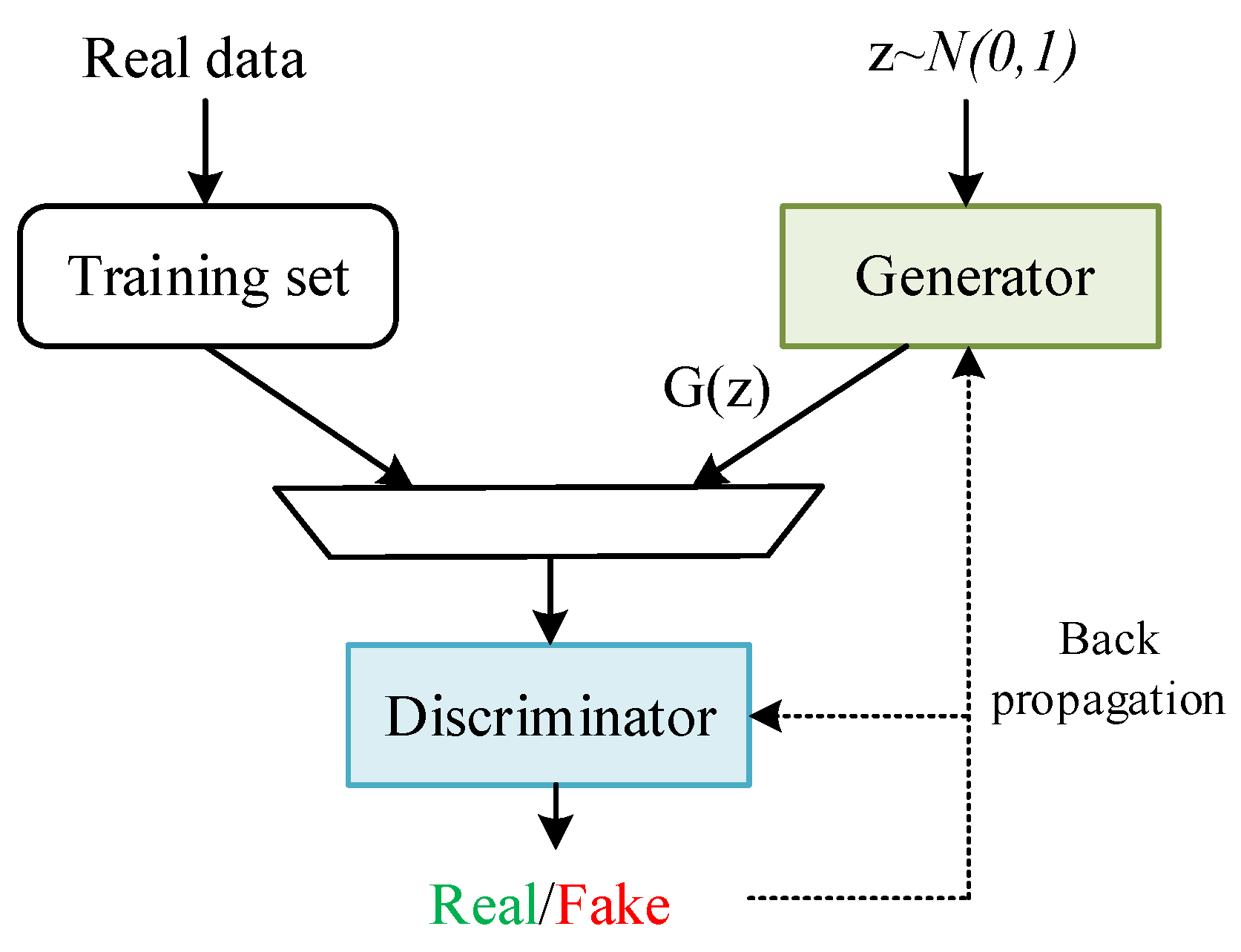
Figure 1. Brief block diagram for the GAN.
Symmetry 17 01489 g001
Figure 2. Working flow of the GAN training process for the clutter data.
Symmetry 17 01489 g002
Figure 3. Construction of 2D pulse-range (spatiotemporal) feature vectors.
Symmetry 17 01489 g003
Figure 4. The architecture of the generator with the axial attention module.
Symmetry 17 01489 g004
Figure 5. Components of the pulse-range (spatiotemporal) axial attention block.
Symmetry 17 01489 g005
Figure 6. Low sea state; a 3D visual comparison of real data and generated data.
Symmetry 17 01489 g006
Figure 7. High sea state; a 3D visual comparison of real data and generated data.
Symmetry 17 01489 g007
Figure 8. High sea state; a 2D heatmap visual comparison between real data and generated data.
Symmetry 17 01489 g008
Figure 9. High sea state; a PCA comparison between real data and generated data.
Symmetry 17 01489 g009
Figure 10. High sea state amplitude comparison of real data and generated data.(ac) epoch = 100. (df) epoch = 1000. (gi) epoch = 3660.
Symmetry 17 01489 g010
Figure 11. Illustration of a 2D heatmap visual comparison between the real and generated data under high sea conditions.
Symmetry 17 01489 g011
Figure 12. Axial attention ablation experiment; PCA comparison between real data and generated data.
Symmetry 17 01489 g012
Figure 13. A pulse signal and its spectrum of real data and generated data.
Symmetry 17 01489 g013
Table 1. Parameters of the radar.
Technical SpecificationParameter
BandX
Frequency Range9.3–9.5 GHz
Range Coverage0.0625–96 nm
Scan Bandwidth25 MHz
Range Resolution6 m
Pulse Repetition Frequency1.6 K, 3 K, 5 K, 10 K
Peak Transmit Power100 W
Antenna Rotation Speed2, 12, 24, 48 rpm
Antenna Length1.8 m (HH), 2.4 m (VV)
Horizontal Beamwidth1.2°
Vertical Beamwidth22°
Transmit Time40 nm–100 μ s
Table 2. Axial attention ablation experiment, mean squared error (MSE) of the statistical histograms between real data and generated data, the Chi-Square ( χ 2 ) test on PDFs, and the Kolmogorov–Smirnov (K-S) test on CDFs. Bold values indicate the best results in each column.
MethodRealImaginaryAmplitude
MSE K-S MSE K-S MSE K-S
Without Axial Attention0.0730.0730.1280.0710.2210.129
All kept (Ours)0.0300.0390.0520.0310.1920.096
Table 3. Resource comparison between standard Multi-Head Self-Attention (MHSA) and axial attention.
Attention TypeComplexityTime per Epoch (s)Memory (GB)Inference Time (s)
Standard MHSA O ( N 2 ) 5979 23.79 1.02
Axial Attention O ( P N + R N ) 4325 16.9 0.80
Table 4. Axial attention ablation experiment; absolute error between the generated data’s power spectral density parameters and real data. Bold values indicate the best results in each column.
Namea μ σ
Without Axial Attention0.03420.24960.0382
All kept (Ours)0.06360.10470.0338
Table 5. Model comparison experiment; mean squared error (MSE) of the statistical histograms between real data and generated data, the Chi-Square ( χ 2 ) test on PDFs, and the Kolmogorov–Smirnov (K-S) test on CDFs. Bold values indicate the best results in each column.
MethodRealImaginaryAmplitude
MSE K-S MSE K-S MSE K-S
AR0.1030.1060.1050.1390.1130.201
WaveGAN0.0950.0960.2050.0890.3160.188
Diffusion0.0460.0510.1440.0710.3020.112
Ours0.0300.0390.0520.0310.1920.096
Table 6. Model comparison experiment; absolute error between the generated data’s power spectral density parameters and real data. Bold values indicate the best results in each column.
Namea μ σ
AR0.15360.34210.1718
WaveGAN0.13980.28120.1516
Diffusion0.08860.26750.1018
Ours0.06360.10470.0338
Table 7. The cosine similarity (Cos-Sim) and Jensen-Shannon distance (Js-Dis) between generated and real data. Bold values indicate the best results in each column.
MethodRealImaginaryAmplitude
Cos-Sim Js-Dis Cos-Sim Js-Dis Cos-Sim Js-Dis
Without Axial
Attention
0.97630.03700.99180.01620.90860.0248
Ours0.99140.00660.99250.00870.99520.0137
Table 8. The cosine similarity (Cos-Sim) and Jensen-Shannon distance (Js-Dis) between the generated and real data. Bold values indicate the best results in each column.
MethodRealImaginaryAmplitude
Cos-Sim Js-Dis Cos-Sim Js-Dis Cos-Sim Js-Dis
AR0.85650.14320.90370.10730.91120.1055
WaveGAN0.96790.08810.97640.06470.92710.0371
Diffusion0.94940.07670.92870.05750.97990.359
Ours0.99140.00660.99250.00870.99520.0137
Disclaimer/Publisher’s Note: The statements, opinions and data contained in all publications are solely those of the individual author(s) and contributor(s) and not of MDPI and/or the editor(s). MDPI and/or the editor(s) disclaim responsibility for any injury to people or property resulting from any ideas, methods, instructions or products referred to in the content.