Bi-xLSTM-Informer for Short-Term Photovoltaic Forecasting: Leveraging Temporal Symmetry and Feature Optimization

Abstract

Exploiting inherent symmetries in data and models is crucial for accurate renewable energy forecasting. To address limited accuracy improvements under complex temporal dependencies, this study proposes a hybrid Bi-xLSTM-Informer model that incorporates temporal symmetry via bidirectional processing of time-flipped sequences. First, key features are screened using the Boruta algorithm, followed by PCA dimensionality reduction to construct an optimal feature subset with orthogonal transformation properties. Second, a Bi-xLSTM-Informer hybrid forecasting model is constructed. In the xLSTM model, the mLSTM is modified into a bidirectional network structure to capture short-term fluctuation patterns via forward and time-reversed propagation; Informer then analyzes global dependencies via ProbSparse attention. Validated on data from the photovoltaic (PV) Power Plant AI Competition, the experimental results demonstrate that the Bi-xLSTM-Informer model achieves the best prediction performance and the lowest error among all compared models, with an R² of 98.76% and an RMSE of 0.3776. This work proves that explicitly modeling temporal symmetry and feature orthogonality significantly enhances PV forecasting, providing an effective solution for renewable energy utilization.

1. Introduction

Driven by the energy transition and the “dual carbon” goals, Photovoltaic (PV) systems significantly reduce air pollution by producing clean energy, while helping to reduce reliance on primary raw materials and traditional energy sources, thus providing strong support for the development of a circular economy [1,2]. However, the intermittent and unpredictable nature of PV power generation poses significant challenges to the stable operation of power systems, electricity market transactions, and the operational management of new energy power plants [3]. Consequently, accurate prediction of PV power generation is of paramount practical importance for optimizing grid operation, ensuring power system stability, and ultimately advancing sustainable development goals [4,5].

PV power generation forecasting can be categorized by time scale into ultra-short-term forecasting (0–24 h), short-term forecasting (24–72 h), and medium- to long-term forecasting (1–12 months) [6]. In comparison to medium- to long-term forecasting, short-term forecasting offers a narrower time horizon and higher prediction accuracy, allowing it to effectively capture the rapid fluctuations in PV power and provide precise data support for real-time grid dispatch [7].

Currently, PV power prediction methods can be classified into physical models, statistical models, and artificial intelligence methods [8]. Physical models depend on complex meteorological parameters and equipment characteristics, but their generalization capability is limited in unstructured scenarios [9]. Statistical models, such as ARIMA [10] and SVM [11], excel at handling linear relationships but face difficulties in capturing nonlinear features and multivariate coupling relationships. With the rapid advancement of artificial intelligence technologies, they have progressively become a focal point of research in the field of PV power prediction [12]. References [13,14] utilizes long short-term memory networks (LSTM) for PV power prediction, and the results indicate that LSTM models can reduce prediction errors. However, LSTM has inherent issues when processing extremely long sequences, such as information loss, gradient vanishing, gradient explosion, and slow training speed. The latest xLSTM architecture effectively overcomes the inherent limitations of LSTM by introducing the exponential gating mechanism and matrix memory unit. It achieves significant improvements in both model expressive capability and parallel computing efficiency, rendering it more adaptable to the complex fluctuation characteristics of PV power. Reference [15] further integrates convolutional neural networks to extract spatial features and combines them with LSTM to form a hybrid model. While this approach enhances gradient stability, it overlooks the importance of feature selection, which ultimately reduces model prediction accuracy. Reference [16] constructed a model embedding layer by extracting relevant features and employed the Informer model for PV generation prediction. However, the Informer model has high demands for input data quality, and its predictive performance can degrade under extreme conditions, such as very small data volumes or high noise levels. To address these challenges, recent studies have primarily adopted hybrid prediction models to achieve complementary optimization by integrating the strengths of multiple methods. Relevant research has mainly concentrated on two key areas: data preprocessing and prediction model construction. By enhancing data quality and feature representation capabilities, the accuracy and robustness of predictions have been significantly improved.

In the data preprocessing stage, PV power generation is influenced by both meteorological factors and equipment operating factors. From the perspective of power generation principles, meteorological factors directly or indirectly affect power generation capacity by influencing key stages of PV conversion; equipment operating factors, on the other hand, impact output power by altering the performance of light absorption or electrical energy conversion pathways. This results in raw data containing a wealth of relevant features, but also containing redundant information, which can lead to reduced prediction accuracy [17]. Therefore, effective feature selection methods are crucial for improving the performance of PV prediction models. Reference [18] employed the Pearson correlation coefficient (PCC) to filter the original input features, which effectively eliminated the influence of weakly correlated variables while conserving computational resources. However, this approach faces limitations when dealing with data containing strongly correlated variables. Reference [19] utilized the Maximal Information Coefficient (MIC) to extract features relevant to PV power generation, though its parameter selection process is somewhat subjective. Reference [20] proposes the use of principal component analysis (PCA) to construct a mixed prediction model, but it has limitations such as the inability to effectively identify key features and difficulty in capturing nonlinear relationships. Reference [21] employs the Boruta algorithm based on the wrapper method for feature selection, which improves wind speed prediction performance. However, the feature set selected by the Boruta algorithm may contain redundant features, necessitating further optimization. Considering a single feature selection method alone is insufficient to balance feature importance and redundant feature removal, adopting a feature combination strategy emerges as a viable solution direction.

PV power generation exhibits inherent temporal patterns that possess approximate time-translation symmetry. To enhance prediction accuracy by addressing the dual challenges of complex temporal dependencies and symmetry exploitation, we propose the Bi-xLSTM-Informer model. The main contributions are

(1)

To address the issue of redundant features in PV data, this study proposes a feature selection method based on Boruta-PCA. The Boruta algorithm is used to evaluate feature importance based on random forests, screening out feature variables significantly correlated with the target variable. PCA transformation constructs an orthogonal feature subspace, removing redundant correlations and creating a symmetric, decorrelated representation that enhances model generalization. This feature optimization method reduces interference from redundant information while overcoming the limitations of traditional single feature extraction methods.

(2)

A Bi-xLSTM-Informer hybrid model explicitly incorporating temporal symmetry via a bidirectional mLSTM layer processing time-flipped sequences. Within the xLSTM framework, the sLSTM structure is retained, and a bidirectional mLSTM processing layer is constructed. Through sequence flipping operations, reverse inputs are generated, and feature concatenation and convolutional fusion are used to enhance bidirectional feature extraction capabilities. The Informer module’s sparse self-attention mechanism captures long-term dependencies in time-series data, enhancing the model’s robustness in modeling nonlinear time-series features. The combination of these two components enables the model to extract effective information across different time scales, thereby improving prediction accuracy.

(3)

A comparative experiment was conducted using data from the PV Power Station Artificial Intelligence Operations and Maintenance Big Data Processing and Analysis Competition, comparing and analyzing eight benchmark models (LSTM-Informer, xLSTM, LSTM, xLSTM-Informer, xLSTM-iTransformer, iTransformer and Informer) to validate that the proposed prediction method achieves higher accuracy.

2. Bi-xLSTM-Informer Prediction Model

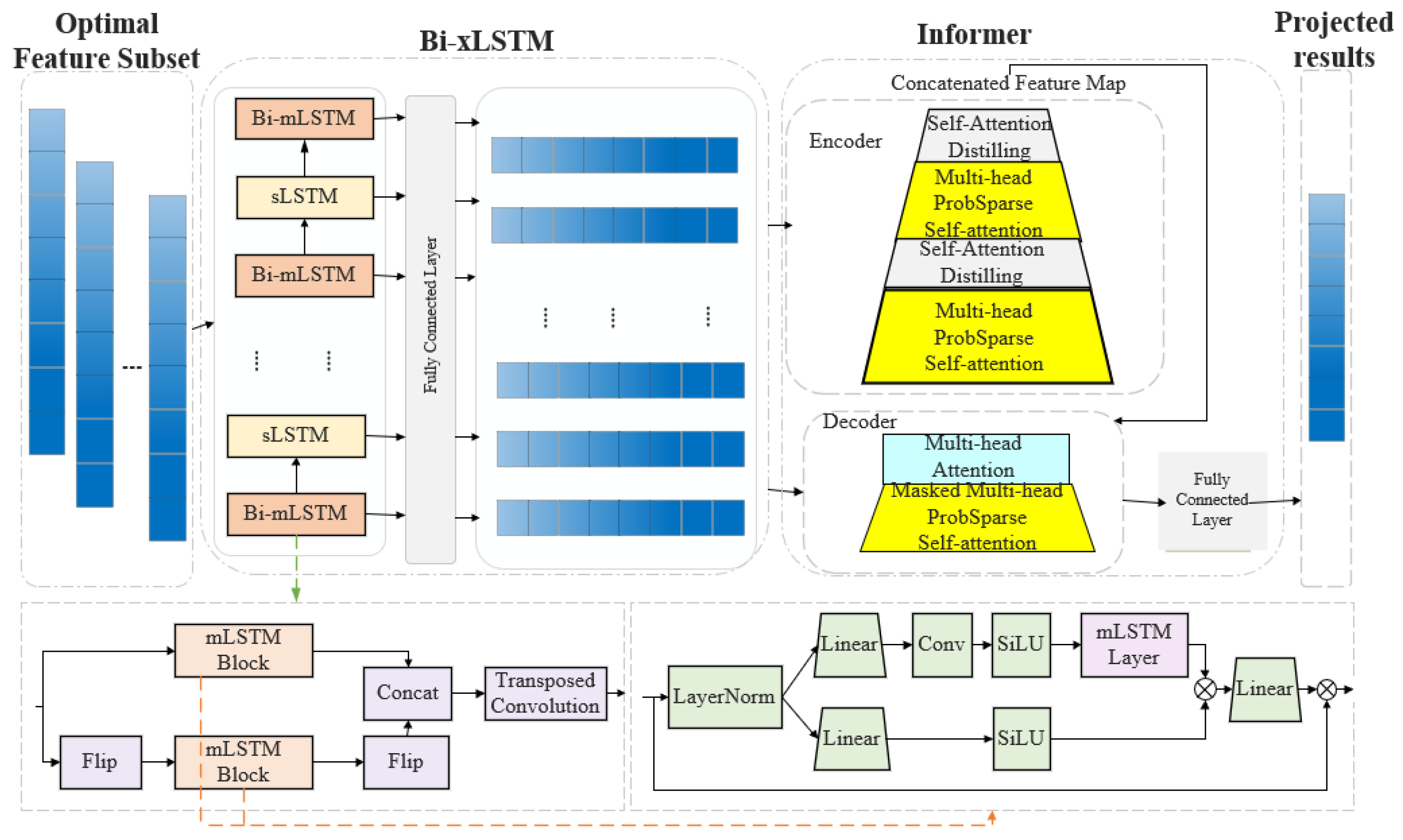
This study introduces the Bi-xLSTM-Informer model to tackle the issues of feature redundancy and the limited improvement in prediction accuracy in PV power forecasting. The general architecture of the model is illustrated in Figure 1. The prediction process is outlined as follows:

The Bi-xLSTM module, consisting of sLSTM and Bi-mLSTM components, is employed to extract local features from the input sequence. Specifically, sLSTM captures short-term dependencies within the sequence, while the Bi-mLSTM layer enhances contextual awareness by simultaneously processing both the forward and reverse sequences—generated through the Flip operation—using the same mLSTM block. The fused local features are subsequently fed into the Informer module, which conducts global dependency analysis on the sequence data. This module also reduces prediction errors through a dynamic compensation mechanism, further enhancing overall prediction accuracy. Finally, the global features are mapped via a fully connected layer to produce the PV power prediction values.

3. Feature Optimization Based on Boruta-PCA

3.1. Boruta Algorithm

The Boruta algorithm is grounded in the principle of random forests, which can effectively capture complex relationships, handle high-dimensional data, and ensure the stability and robustness of feature selection through multiple sampling evaluations. Its core concept is to generate “shadow features” for each original feature in the data. By comparing the importance of the original features with the shadow features, the algorithm identifies and selects the truly significant features [22].

The main steps are as follows:

(1)

Copy the original feature data and randomly shuffle it to generate the corresponding shadow features.

(2)

Merge the original features with the shadow features to form a new set of features.

(3)

Input the new feature set into the random forest model and calculate the importance score of each characteristic. The calculation formula is as follows [23]:

$$Z_{\mathrm{s}\mathrm{c}\mathrm{o}\mathrm{r}\mathrm{e}}={\displaystyle \frac{MS{E}_{\mathrm{O}\mathrm{O}\mathrm{B}}}{SDMS{E}_{\mathrm{O}\mathrm{O}\mathrm{B}}}}$$

(1)

where $Z_{\mathrm{s}\mathrm{c}\mathrm{o}\mathrm{r}\mathrm{e}}$ is the score, $MS{E}_{\mathrm{O}\mathrm{O}\mathrm{B}}$ is the average out-of-bag error of the random forest, and $SDMS{E}_{\mathrm{O}\mathrm{O}\mathrm{B}}$ is the standard deviation of the out-of-bag error.

(4)

Take the maximum Z-score of all shadow features as the importance threshold. If the Z-score of an original feature exceeds this threshold, the feature is deemed important; otherwise, it is considered unimportant and permanently removed from the feature set.

(5)

Repetition of Steps 3 and 4 occurs until all features are classified as either “important” or “unimportant”.

3.2. Principal Component Analysis (PCA)

To eliminate redundant information in the measured features after feature importance screening, this study employs PCA to perform dimensionality reduction on the feature data, thereby extracting important and mutually independent key features. PCA performs an orthogonal transformation of selected features, projecting them into a new coordinate system defined by eigenvectors (principal components). This creates a symmetric, uncorrelated feature space where dimensions are linearly independent, effectively reducing multicollinearity and enhancing model stability. The new features are linear combinations of original variables, with principal components mutually independent [24]. In this study, principal components with cumulative contribution rates exceeding 95% are identified as the reduced-dimension feature set, ensuring that while significantly reducing the dimension, the key information critical to the prediction task is maximally retained.

4. Bi-xLSTM and Informer Models

4.1. Bi-xLSTM Model

To clearly illustrate the core recurrent neural network architecture discussed in this paper and its evolutionary relationship,

Table 1. Overview of LSTM-based Models and Their Characteristics.

Model	Core Concept	Problem Solved
LSTM	A recurrent neural network variant introducing a gating mechanism and a cell state to enable selective retention and forgetting of information. It serves as a foundational benchmark for sequence modeling.	Addresses the vanishing or exploding gradient problem of simple RNNs, thereby capturing long-term dependencies in sequences.
sLSTM	A variant within the xLSTM framework. Its core lies in retaining and enhancing the scalar memory structure of traditional LSTM, while supporting a multi-head architecture to improve model capacity.	Enhances the expressive power and information utilization efficiency of traditional LSTM, and overcomes the limitations of its sigmoid gating.
mLSTM	Another variant in the xLSTM framework. Its core innovation is replacing scalar memory with matrix memory units and covariance update rules to achieve fully parallel computation; its key-value pair query mechanism is direction-agnostic.	Breaks the sequential computation bottleneck of LSTM, enables parallelization, and significantly expands memory capacity.
xLSTM	An integrated architecture that combines sLSTM blocks and mLSTM blocks through residual stacking. It inherits the strong sequence modeling capability of the former, as well as the efficient parallelism and large memory capacity of the latter.	Effectively overcomes the limitations of LSTM in terms of expressiveness, parallelism, and memory capacity.

compares the core concepts and features of LSTM and its extended versions (sLSTM, mLSTM) as well as the overall xLSTM framework.

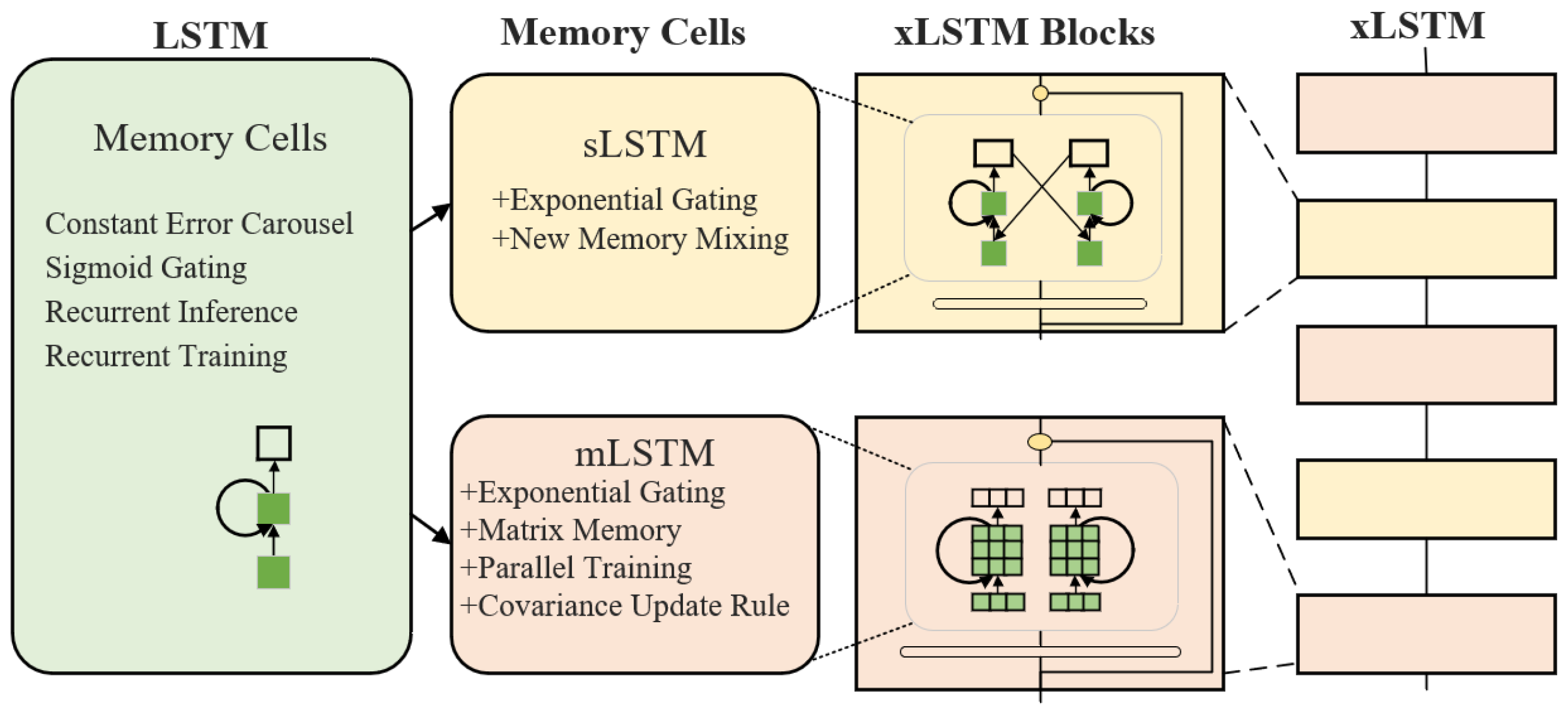
xLSTM is an extended architecture based on the traditional LSTM network. By incorporating an exponential gating mechanism, designing a novel memory structure, and adopting a residual stacking architecture, it significantly enhances performance in sequence prediction tasks [25]. xLSTM includes two new variants: sLSTM and mLSTM.

The complete xLSTM architecture is composed of several xLSTM blocks arranged sequentially, with each block being constructed by alternately stacking sLSTM and mLSTM blocks. The overall configuration is illustrated in Figure 2.

sLSTM retains the scalar memory unit while introducing new memory mixing techniques and layer normalization state constraints—allowing memory units to mix information across layers and improving information storage and utilization efficiency. In contrast, mLSTM uses matrix-form memory units and optimizes storage strategies via covariance update rules, enabling dynamic adjustment of matrix parameters to adapt to data features and enhancing storage capacity and sparse information retrieval. Additionally, mLSTM eliminates connections between hidden states across time steps, breaking the sequential computation pattern of traditional LSTMs and enabling fully parallel processing. The forward propagation formula of mLSTM is as follows [26]:

$$C_t= {\mathrm{f}}_t{C}_{t-1}+ {\mathrm{i}}_t v_t{k}_t^{\mathrm{\top }}$$

(2)

$$n_t={\mathrm{f}}_t{n}_{t-1}+{\mathrm{i}}_t{k}_t$$

(3)

$$h_t=o_t\odot \left({\displaystyle \frac{C_t{q}_t}{\max \left(\right|n_t^{\mathrm{\top }}{q}_t|,1)}}\right)$$

(4)

$$q_t=W_q{x}_t+b_q$$

(5)

$$k_t={\displaystyle \frac{1}{\sqrt{d}}}{W}_k{x}_t+b_k$$

(6)

$$v_t=W_v{x}_t+b_v$$

(7)

$${\mathrm{i}}_t=\mathrm{e}\mathrm{x}\mathrm{p}\left(w_{\mathrm{i}}^{\mathrm{\top }}{x}_t+b_{\mathrm{i}}\right)$$

(8)

$${\mathrm{f}}_t=\exp \left(w_{\mathrm{f}}^{\mathrm{\top }}{x}_t+b_{\mathrm{f}}\right)$$

(9)

$$o_t=\sigma \left(W_o{x}_t+b_o\right)$$

(10)

where $C_t$ is the current cell state, $n_t$ is the normalized state, $h_t$ is the hidden state, $o_t$ is the output gate, $v_t$ is the value vector, $k_t$ is key vector, $q_t$ is the query vector, ${\mathrm{i}}_t$ is the input gate, and ${\mathrm{f}}_t$ is the forget gate.

Traditional xLSTM networks use a unidirectional sequential training method when processing PV power generation time series data, which limits the ability to fully explore the temporal dependencies within the data. The bidirectional architecture lets the model process sequence data from both forward and backward directions simultaneously, enabling more comprehensive capture of contextual dependencies in the input sequence. In variants of xLSTM, sLSTM relies on memory mixing through recurrent connections, which supports multi-head architectures.

However, intra-head memory mixing requires sequential sequence processing, and bidirectional adaptation necessitates cross-head communication, potentially increasing design complexity. In contrast, the mLSTM network is based on a matrix memory structure and covariance update rules. Its key-value pair storage and query mechanism has direction-independent characteristics, meaning that bidirectional expansion does not disrupt the original mathematical structure. This design feature allows mLSTM to significantly enhance language modeling performance after bidirectional adaptation.

Based on this, this study proposes a Bi-xLSTM model, which consists of an sLSTM network and a Bi-mLSTM network. In the Bi-mLSTM network, a unidirectional mLSTM block with shared parameters is used to process reverse sequences through a flip operation. The bidirectional outputs are concatenated and integrated with a Conv1D convolution to achieve feature extraction. This mechanism enables the Bi-xLSTM model to simultaneously capture both forward and reverse temporal features of the data, efficiently uncovering the intrinsic connections between current data and past/future data, thereby improving data utilization efficiency and prediction accuracy. The computational formula for the Bi-xLSTM network structure is

$$v=\mathrm{C}\mathrm{o}\mathrm{n}\mathrm{v}1\mathrm{D}\left(\mathrm{m}\mathrm{L}\mathrm{S}t\mathrm{M}\left(\theta \right)\oplus \mathrm{m}\mathrm{L}\mathrm{S}t\mathrm{M}\left(\mathrm{f}\mathrm{l}\mathrm{i}\mathrm{p}\left(\theta \right)\right)\right)$$

(11)

where $\mathrm{f}\mathrm{l}\mathrm{i}\mathrm{p}\left(\theta \right)$ operation generates a time-reversed copy of the input sequence, enabling the model to learn temporally symmetric representations. This is critical for capturing invariant patterns under time-direction transformations.The structure of the Bi-mLSTM model is illustrated in Figure 3.

In addition, traditional LSTMs rely on sigmoid gate functions for information control, with output values constrained to the range [0, 1], which presents certain limitations. xLSTM adopts an exponential activation function, allowing the input and forget gates to control memory updates exponentially—enabling more efficient information flow and memory adjustments. This lets the model make more significant changes to the memory cell state, quickly integrating new information and adjusting its memory accordingly.

4.2. Informer

Due to the inherent challenges in parallelizing certain components when handling long sequences, the performance of xLSTM is somewhat constrained. Consequently, this study incorporates the Informer model, to achieve superior prediction results. The Informer model is founded on the Transformer architecture, replacing the conventional self-attention mechanism with the ProbSparse self-attention mechanism. This modification substantially streamlines the computational process, reducing both computational and space complexities from O(L²) to O(lgL), thereby enhancing the model’s efficiency and effectively mitigating resource constraints when processing extended sequences [27].

In long sequence modeling, only a small subset of key vectors exerts a substantial influence on each query vector, meaning the attention distribution is sparse. Leveraging this characteristic, Informer introduces the ProbSparse self-attention mechanism, which utilizes KL divergence to assess the sparsity of the i-th query vector $q_i$:

$$\overline{M}\left(q_i,k\right)=\underset{j}{max}\left\{{\displaystyle \frac{q_i{k}_j^T}{\sqrt{d}}}\right\}-{\displaystyle \frac{1}{L_K}}\sum _{j=1}^{L_K}{\displaystyle \frac{q_i{k}_j^T}{\sqrt{d}}}$$

(12)

where $q_i$,$k_i$ represent the i-th row of Q and K, respectively.

After computing the “sparsity score”, a new sparse query matrix is selected, consisting of the top-u query vectors with the highest sparsity scores. The average value is then directly assigned to the remaining query vectors. Finally, the ProbSparse self-attention is computed as follows:

$$\mathrm{Sparse} \mathrm{Attention} \left(Q,K,V\right) = \mathrm{softmax}\left({\displaystyle \frac{Q^{\prime }{K}^{\mathrm{T}}}{\sqrt{\mathrm{d}}}}\right)V$$

(13)

where $Q^{\prime }$ is the sparse query matrix.

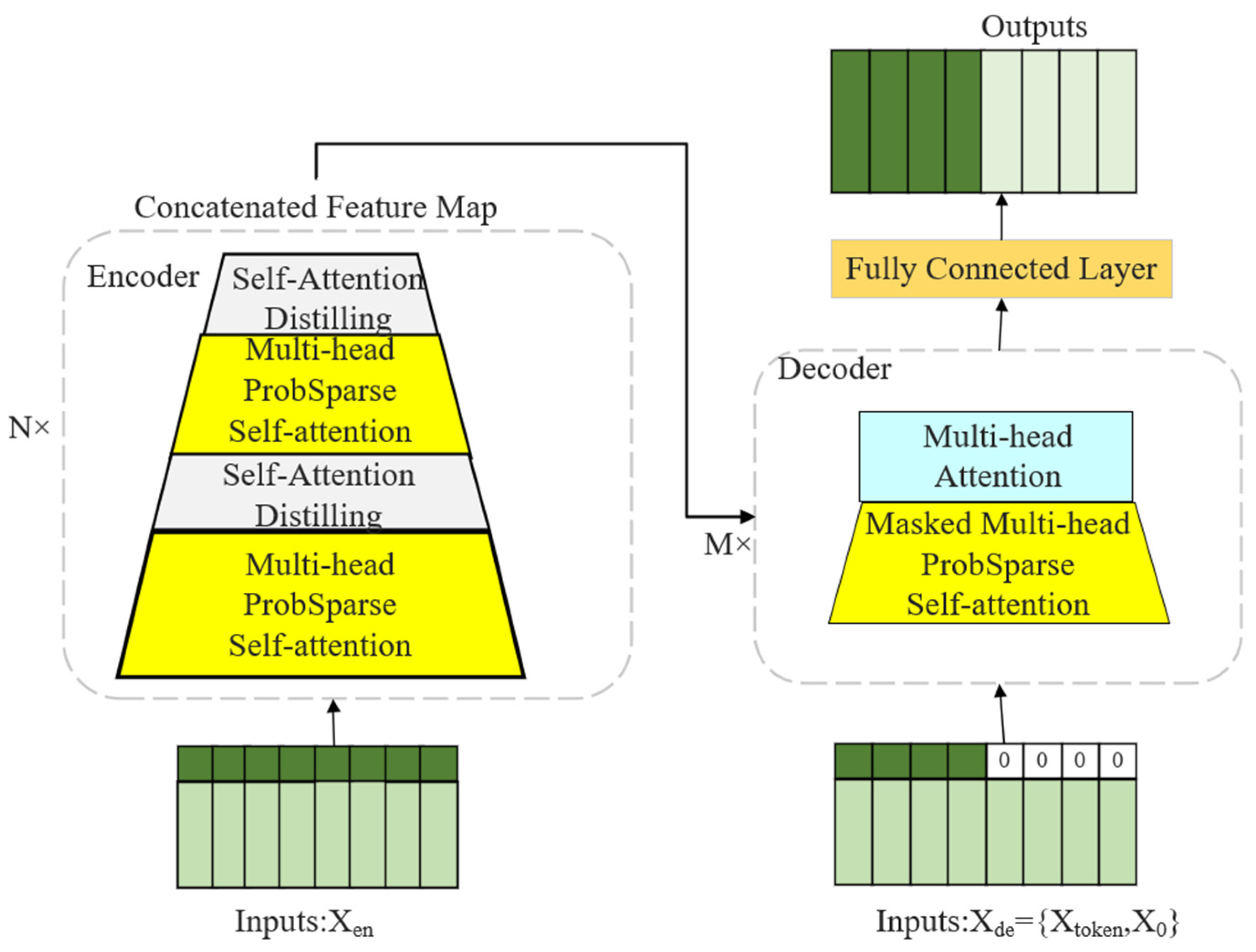
Informer consists of an encoder and a decoder, with the model architecture depicted in Figure 4. The encoder is made up of several stacked encoding layers, each primarily comprising a ProbSparse self-attention module and a feedforward neural network module. The encoder processes the input long-sequence time series data to capture long-term dependency features.

Furthermore, a self-attention distillation operation is incorporated within the encoder, where the input to each subsequent layer is halved to extract the dominant attention, allowing the Informer to effectively manage exceptionally long input sequences. The distillation formula from the first layer to the final layer is as follows:

$${X }_{j+1}^t = {\mathrm{Max}}_{\mathrm{pool}}(\mathrm{ELU}\left(\mathrm{Conv}-1\mathrm{d}\left([{X }_j^t{]}_{\mathrm{AB}}\right)\right)$$

(14)

where $\mathrm{Conv}-1\mathrm{d}$ is the one-dimensional convolution operation, $\mathrm{ELU}$ is the activation function, and ${\mathrm{Max}}_{\mathrm{pool}}$ is the maximum pooling operation.

The decoder is also composed of multiple stacked decoding layers, each containing a cross-attention module, a ProbSparse self-attention module, and a feedforward neural network module. The decoder predicts future time series values based on the encoder’s output and previously predicted outputs. That is,

$${X }_{f d}^t=\mathrm{Concat} \left({X }_P^t+{X }_t^t\right) \in {\mathrm{R}}^{\left(L_{token}+L_y\right)\times d_{model}}$$

(15)

where ${X }_{f d}^t$ is the input sequence of the decoder, ${X }_t^t$ is the start token, and ${X }_P^t$ is the target placeholder.

5. Experimental Results and Analysis

5.1. Experimental Procedure

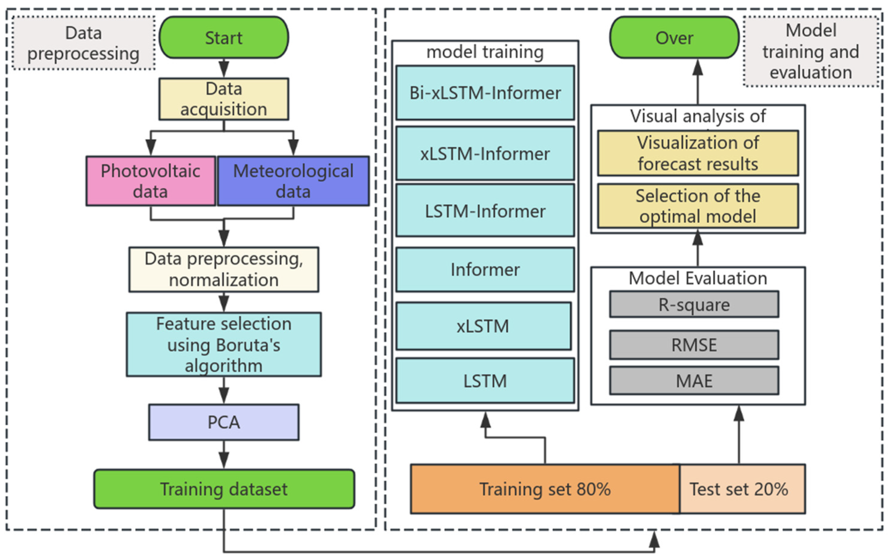
The prediction process of this study is illustrated in Figure 5, and the specific experimental steps are as follows: First, PV and meteorological data are collected and preprocessed. Next, the Boruta algorithm is employed for preliminary feature selection to identify the most predictive features. PCA is then applied to reduce the dimensionality of the selected features and eliminate redundant information, ultimately forming an optimized feature set for the construction of the training dataset. Finally, the dataset is split into training and testing sets, and various models are used for experimentation. Evaluation metrics are utilized to assess the performance of each model, with the optimal model being selected based on the prediction results.

5.2. Data Description and Preprocessing

5.2.1. Data Description

(1)

Primary Dataset (Dataset 1): Short-Term Operational Data

The dataset used in this study was sourced from the Artificial Intelligence Operation and Maintenance Big Data Processing and Analysis Competition for PV Power Plants [28], which provided operational data from a real-world PV system in China. It records high-resolution temporal data from three monitoring points alongside meteorological parameters over 45 days, comprising 9000 data points. These data include conversion efficiency, voltage, current, and power, which were randomly selected from three monitoring points (A, B, and C). Equipment operational status parameters, such as the back-side temperature of PV modules and average conversion efficiency, are included. The dataset includes environmental data from the power plant site, such as temperature, irradiance, wind speed, and wind direction.

(2)

Supplementary Dataset (Dataset 2): Long-Term Seasonal Data

To comprehensively evaluate the model’s generalization capability under long-term seasonal variations, we employed a supplementary dataset from a solar power station in China [29]. This dataset spans two full years (1 January 2019 to 31 December 2020) with a temporal resolution of 15 min, providing a much longer time horizon that encapsulates full seasonal cycles. It includes key meteorological and power generation metrics such as global horizontal irradiance, ambient temperature, wind speed, and humidity. This dataset is exclusively used in Section 5.5.5 to validate the model’s robustness to seasonal changes.

5.2.2. Data Preprocessing

During the data preprocessing stage, the interquartile range (IQR) of box plots is utilized to detect outliers. For missing values, linear interpolation was used to fill them in order to ensure the continuity of the time series. For the identified outliers, the average value of the data points preceding and following the outlier is used for replacement. Subsequently, the Min-Max normalization technique is applied to scale both the input features and the target variable to the range [0, 1], which mitigates the impact of dimensional differences on model training. The formula for Min-Max normalization is as follows:

$$X_{\mathrm{n}\mathrm{o}\mathrm{r}\mathrm{m}}={\displaystyle \frac{X-X_{\mathrm{m}\mathrm{i}\mathrm{n}}}{X_{\mathrm{m}\mathrm{a}\mathrm{x}}-X_{\mathrm{m}\mathrm{i}\mathrm{n}}}}$$

(16)

where $X_{\mathrm{m}\mathrm{a}\mathrm{x}}$ and $X_{\mathrm{m}\mathrm{i}\mathrm{n}}$ represent the maximum and minimum values of the feature columns, respectively.

After this normalization, all input data for subsequent algorithms are converted to dimensionless values. Thus, all mathematical operations related to feature engineering (Section 3) and model computations (Section 4) are dimensionless transformations.

The preprocessing process used in the study is designed to improve data quality and model performance. This study divided the Dataset 1 into an 8:2 ratio and employed a sliding window single-step prediction method to forecast daily PV power generation for days 37 to 45. The predicted results were then compared with the actual observed values to assess the model’s prediction performance.

5.3. Feature Engineering

There are a total of 19 feature factors in the original Dataset 1, including 15 PV panel operating status features and 4 meteorological features.

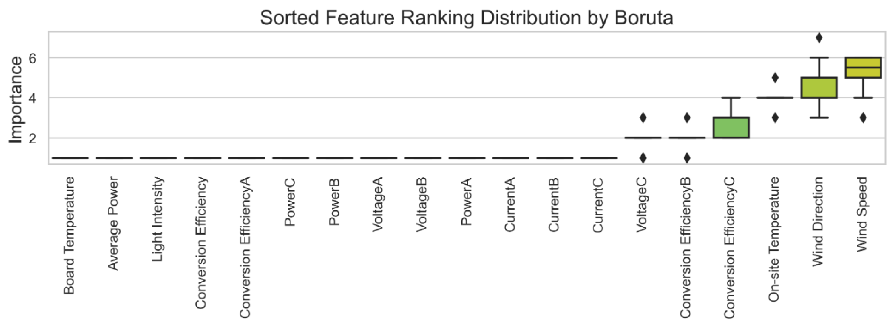
To accurately screen out the core features that have a significant impact on the prediction variables, the Boruta algorithm is first used to perform a preliminary screening of the original feature set. Considering that a single feature ranking may be random, the Boruta algorithm is run multiple times to assess the stability of each feature ranking. The final screening results and feature importance rankings are shown in Figure 6.

The features on the far left of Figure 6 (e.g., plate temperature and average power) consistently rank highly across multiple iterations, indicating their significance in the model. In contrast, the features on the far right (e.g., voltage C and conversion efficiency B) consistently rank low, suggesting their lesser importance in the model, leading to their exclusion.

As a result, the Boruta algorithm identified 13 significant feature variables, ranked from highest to lowest importance as follows: plate temperature, average power, light intensity, conversion efficiency, conversion efficiency A, power C, power B, voltage A, voltage B, power A, current A, current B, and current C.

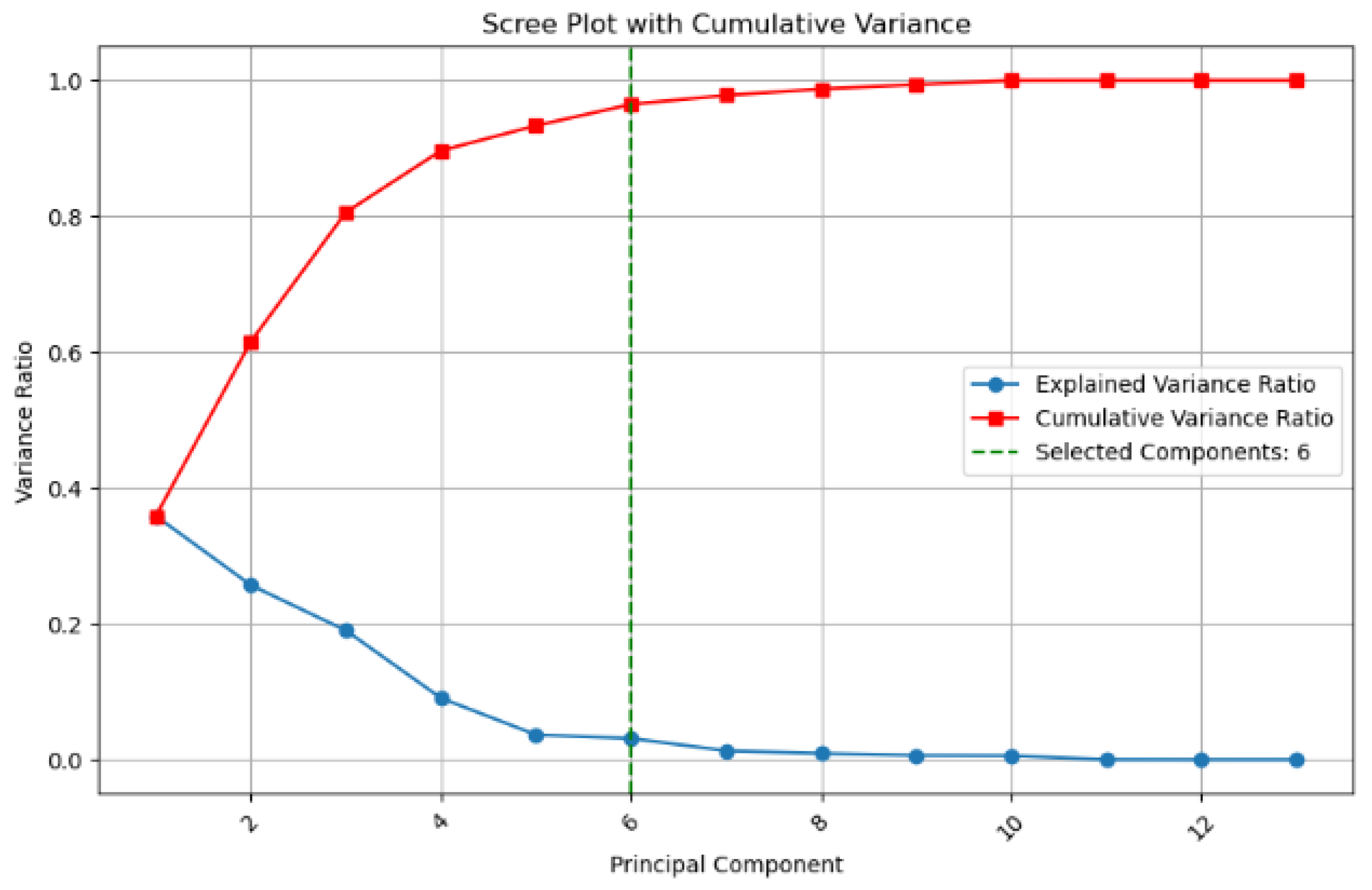
PCA was further applied to reduce the dimensionality of the feature space and eliminate multicollinearity, thereby optimizing the model’s feature input. Based on the principle of cumulative contribution exceeding 95%, the first six principal components were selected as the model’s input features in the PCA-processed feature space. The results are shown in Figure 7.

5.4. Evaluation Indicators

This study selected the Mean Absolute Error (MAE),Root Mean Square Error (RMSE) and the coefficient of determination R² as evaluation metrics to assess the predictive performance of the model [30]. A forecast result is primarily deemed satisfactory based on its ability to achieve comprehensive superiority across all benchmarks, simultaneously demonstrating the lowest MAE, lowest RMSE, and highest R² values. The formulas for these three evaluation indicators are as follows [31] (unit: kW):

$$R^2=1-{\displaystyle \frac{{\sum }_{i=1}^n (y_i-{\widehat{y}}_i{)}^2}{{\sum }_{i=1}^n (y_i-\overline{y}{)}^2}}$$

(17)

$$MAE={\displaystyle \frac{1}{n}}\sum _{i=1}^n \mid y_i-{\widehat{y}}_i\mid$$

(18)

$$RMSE=\sqrt{{\displaystyle \frac{1}{n}}\sum _{i=1}^n (y_i-{\widehat{y}}_i{)}^2}$$

(19)

where $y_i$ is the actual value, ${\widehat{y}}_i$ is the predicted value, and $n$ is the sample size.

5.5. Experimental Results and Comparison

5.5.1. Hyperparameters Settings

The research model hyperparameters were determined through multiple experiments and are shown in

Table 2. Model Hyperparameters Settings.

Name	Hyperparameters
Model hyperparameters	timesteps = 10
	Optimizer = Adam
	Loss function = MAE
	epochs = 100
	lr = 0.0001
	batch_size = 64
xLSTM hyperparameters	xLSTM layers = 3
	Number of neurons per xLSTM layer = 64
Informer hyperparameters	e_layers = 2
	d_layers = 1
	Dropout = 0.1
	d_model = 64

.

5.5.2. Feature Selection Effect

The original features, features screened by the Boruta algorithm, and features selected by Boruta-PCA were input into four models to evaluate the impact of feature selection on the performance of PV power generation prediction models. A comparative analysis was then conducted using the evaluation metrics. The specific results are shown in

Table 3. Model Performance under Different Feature Selection Methods.

Model	Feature Selection Method	R2	MAE	RMSE
LSTM	Original Features	0.91291	0.5767	0.9781
	Boruta Algorithm	0.9193	0.5184	0.9631
	Boruta-PCA	0.9218	0.4564	0.9477
xLSTM	Original Features	0.9197	0.4821	0.9606
	Boruta Algorithm	0.9207	0.4688	0.9548
	Boruta-PCA	0.9244	0.4582	0.9315
Informer	Original Features	0.9485	0.5174	0.7698
	Boruta Algorithm	0.9744	0.2907	0.5428
	Boruta-PCA	0.9824	0.1941	0.4499
xLSTM-Informer	Original Features	0.9493	0.5125	0.7639
	Boruta Algorithm	0.9782	0.2503	0.5004
	Boruta-PCA	0.9860	0.1607	0.4009

.

Compared to the original features, the features selected by the Boruta algorithm significantly improved the performance of all models. Specifically, the R² value of the Informer model increased by 2.73%, while MAE and RMSE decreased by 43.82% and 29.49%, respectively; the R² value of the xLSTM-Informer model increased by 3.04%, while MAE and RMSE decreased by 51.16% and 34.49%, respectively. In comparison, the R² value of the LSTM model increased by 0.70%, while MAE decreased by 10.11% and RMSE decreased by 1.53%. The R² value of the xLSTM model increased by 0.11%, with MAE decreasing by 2.76% and RMSE decreasing by 0.60%. These experimental results demonstrate that the Boruta algorithm can effectively identify features that have a significant impact on model performance, thereby optimizing the feature selection process.

Compared to feature selection using the Boruta algorithm, all models exhibited improved R² values after feature selection with Boruta-PCA, alongside reduced error metrics (MAE and RMSE). Specifically, the R² value of the Informer model increased by 0.82%, while MAE and RMSE decreased by 33.23% and 17.11%, respectively. The R² value of the xLSTM-Informer model increased by 0.80%, with MAE and RMSE decreasing by 35.80% and 19.88%, respectively. In comparison, the R² value of the LSTM model increased by 0.27%, while MAE decreased by 11.96% and RMSE decreased by 1.60%. The R² value of the xLSTM model increased by 0.40%, with MAE decreasing by 2.26% and RMSE decreasing by 2.44%. Experiments show that PCA effectively reduces the data dimension while retaining more than 95% of the original data information, providing more efficient input for subsequent models.

In summary, the two-stage feature optimization of Boruta-PCA significantly improves model prediction accuracy by eliminating redundant feature noise and multicollinearity.

5.5.3. Comparison and Analysis of Different Model Performance

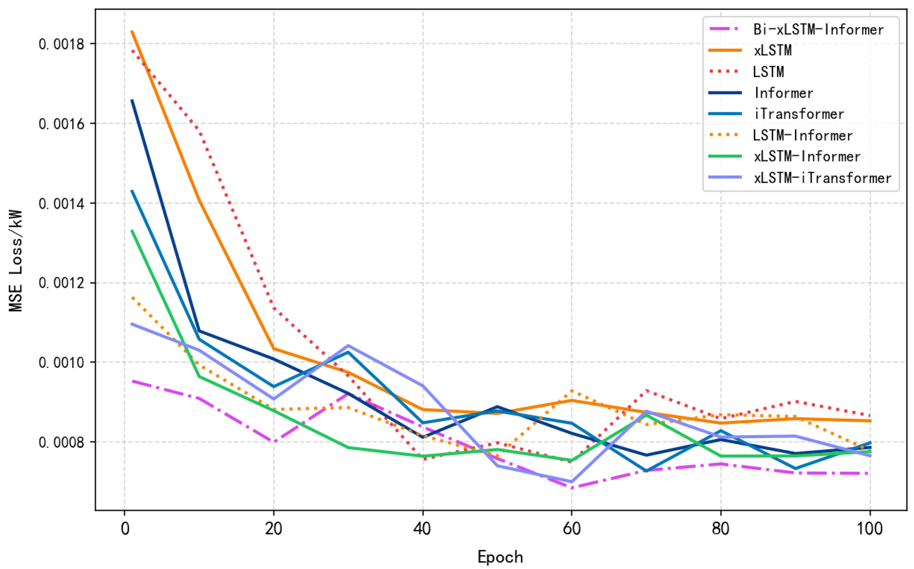
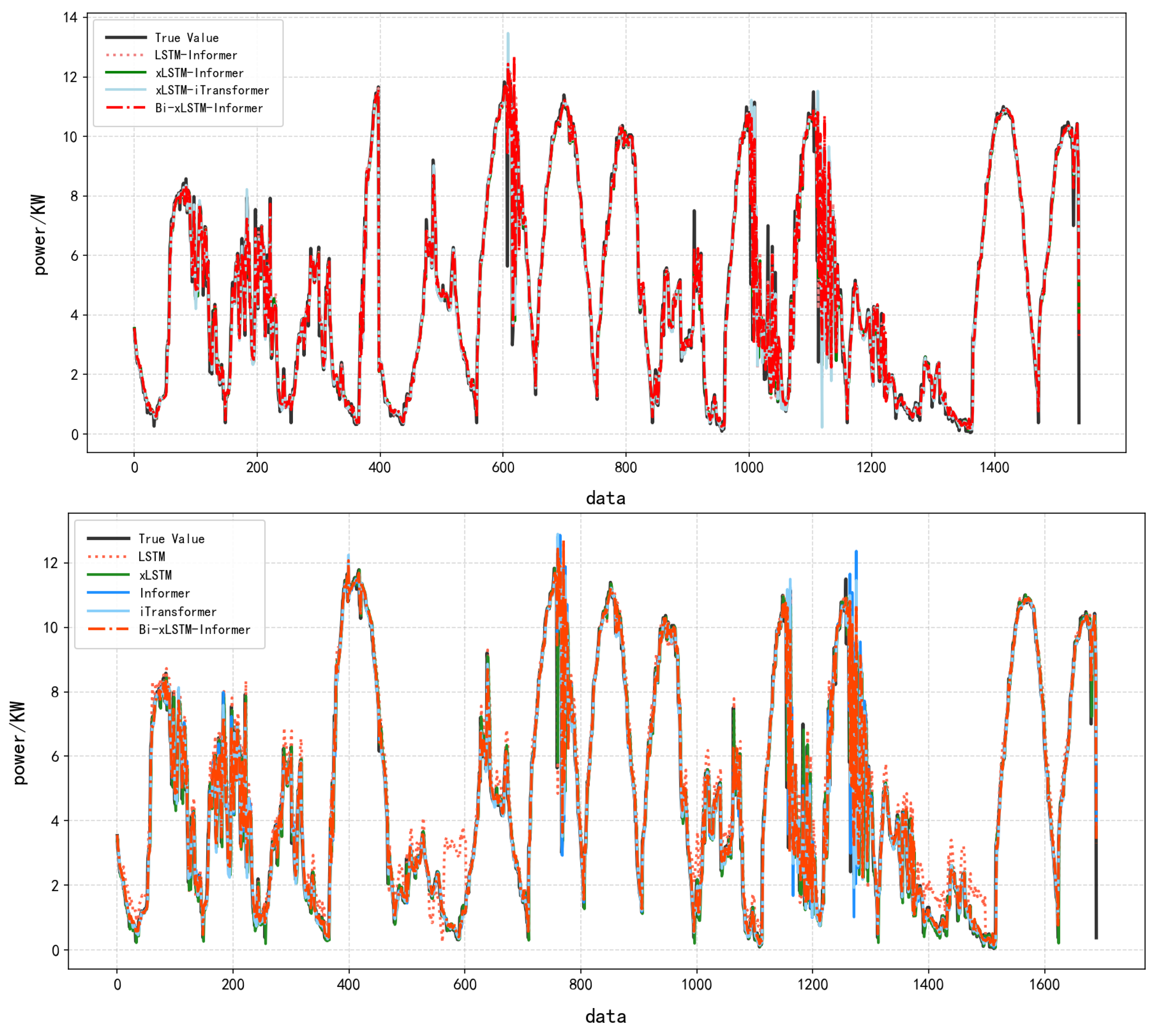
Comparison experiments were conducted using the LSTM, Informer, xLSTM, LSTM-Informer, and xLSTM-Informer models to validate the performance of the Bi-xLSTM-Informer model. The prediction results and prediction errors are presented in

Table 4. Comparison of Effects of Different Models Based on Full Dataset 1.

Model	R2	MAE	RMSE
LSTM	0.9218	0.4564	0.9477
xLSTM	0.9244	0.4582	0.9315
iTransformer	0.9823	0.1952	0.4498
Informer	0.9824	0.1941	0.4499
LSTM-Informer	0.9851	0.1774	0.4128
xLSTM-iTransformer	0.9858	0.1698	0.4085
xLSTM-Informer	0.9860	0.1687	0.4009
Bi-xLSTM-Informer	0.9876	0.1646	0.3776

, Figure 8 and Figure 9, respectively.

As shown in Table 4, the Bi-xLSTM-Informer model achieved R², MAE, and RMSE values of 0.9876, 0.1646, and 0.3776, respectively. Compared to the other models, it exhibited the best fitting performance and the lowest error.

When comparing the prediction results of the Bi-xLSTM-Informer model with those of the LSTM and xLSTM models, it is clear that single prediction models are inadequate for capturing both long-term and short-term dependencies in PV time-series data. This limitation makes it difficult to model complex fluctuations, resulting in poor fitting performance. Upon incorporating the Informer model, prediction accuracy was significantly improved, and the error was notably reduced. For instance, in the case of the xLSTM-Informer model, compared to the xLSTM model, RMSE was reduced by 56.96%, and R² increased by 6.66%. This demonstrates that Informer can more efficiently extract key information from long sequences. However, due to the constraints of a single attention structure, it faces certain limitations in capturing the local details of the data.

Compared to the LSTM-Informer model, the Bi-xLSTM-Informer model improved the R² value by 0.25% and reduced the RMSE by 8.53%. Compared to the xLSTM-iTransformer model, the Bi-xLSTM-Informer model improved the R² value by 0.16% and reduced the RMSE by 5.81%. Compared to the xLSTM-Informer model, the Bi-xLSTM-Informer model improved the R² value by 0.16% and reduced the RMSE by 5.81%. These results indicate that the dynamic gating optimization of xLSTM is better suited to the multi-scale features of PV data than the traditional LSTM. Furthermore, the bidirectional architecture significantly enhances complex feature capture capability, demonstrating that modeling temporal symmetry via bidirectional processing is particularly effective for extracting fluctuations.

5.5.4. Statistical Validation

To confirm that the observed performance gains are statistically significant, a paired sample t-test was conducted to compare the point-wise prediction errors between the proposed Bi-xLSTM-Informer model and all three baseline models (LSTM, xLSTM, Informer) on the test set of Dataset 1. The test was performed based on multiple independent runs for both MAE and RMSE metrics, ensuring the reliability of error comparisons.

The null hypothesis (H₀) posited that there was no significant difference in the mean prediction error between the Bi-xLSTM-Informer and each baseline model, while the alternative hypothesis (H₁) stated that the Bi-xLSTM-Informer model yielded significantly lower mean errors. With a significance level set at α = 0.05, the results (

Table 5. Paired t-test Results of MAE and RMSE on the 45-day Dataset.

Baseline Model	p-Value (MAE)	p-Value (RMSE)	Significance (α = 0.05)
LSTM	1.89 × 10−7	2.63 × 10−6	Significant
xLSTM	1.52 × 10−6	2.17 × 10−5	Significant
Informer	3.94 × 10−4	4.82 × 10−3	Significant

) show that all obtained p-values are far below this threshold.

Therefore, we can confidently reject the null hypothesis for every model comparison. This provides strong statistical evidence that the superior performance of our proposed Bi-xLSTM-Informer model—reflected in lower MAE and RMSE on Dataset 1’s test set—is genuine and not due to random fluctuations in the test data.

5.5.5. Robustness Validation

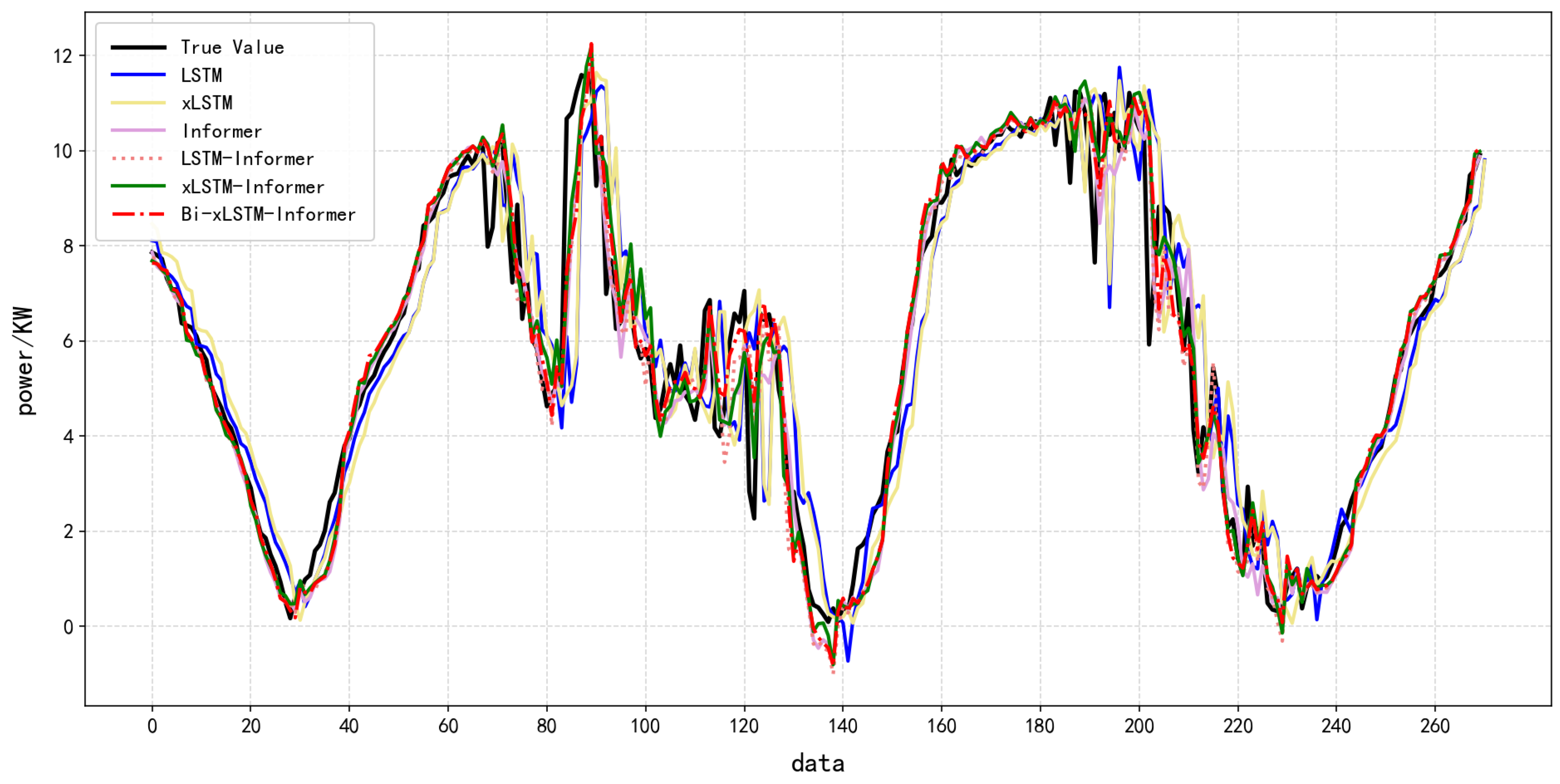
To verify the robustness and generalization ability of the model, this study used random sampling methods to process the dataset. At the same time, to maintain the temporal continuity within the subsamples and avoid distorting the time-dependent relationships caused by random shuffling, seven days of samples were randomly extracted from the dataset and input into the model for independent experiments. The results are shown in

Table 6. Comparison of Effects of Different Models Based on Sample Dataset 1.

Model	R2	MAE	RMSE
LSTM	0.9234	0.5308	0.9029
xLSTM	0.9258	0.5031	0.8942
Informer	0.9384	0.5365	0.8174
LSTM-Informer	0.9407	0.5177	0.8018
xLSTM-Informer	0.9458	0.5104	0.7668
Bi-xLSTM-Informer	0.9483	0.4852	0.7485

and Figure 10. Comparison of Effects of Different Models Based on Sample Dataset 1. The predicted results are shown in Table 6.

The experimental results show that in the PV power prediction task based on sampled data, the Bi-xLSTM-Informer’s consistent performance across sampled datasets 1 highlights its robustness under temporal variations, a benefit attributed to its symmetry-aware architecture which learns invariant patterns. Specifically, the Bi-xLSTM-Informer model demonstrates the highest prediction accuracy: its MAE and RMSE are all lower than those of the five comparison models (LSTM, xLSTM, Informer, etc.), and the fit between the predicted values and the actual values is the highest. Moreover, through multiple replicate experiments, the model demonstrated the smallest variation in prediction errors across different sampled datasets, with its optimal performance occurring significantly more frequently than other models. This indicates the model exhibits excellent robustness in handling temporal data fluctuations and feature redundancy issues.

5.5.6. Validation of Model Adaptability to Seasonal Changes

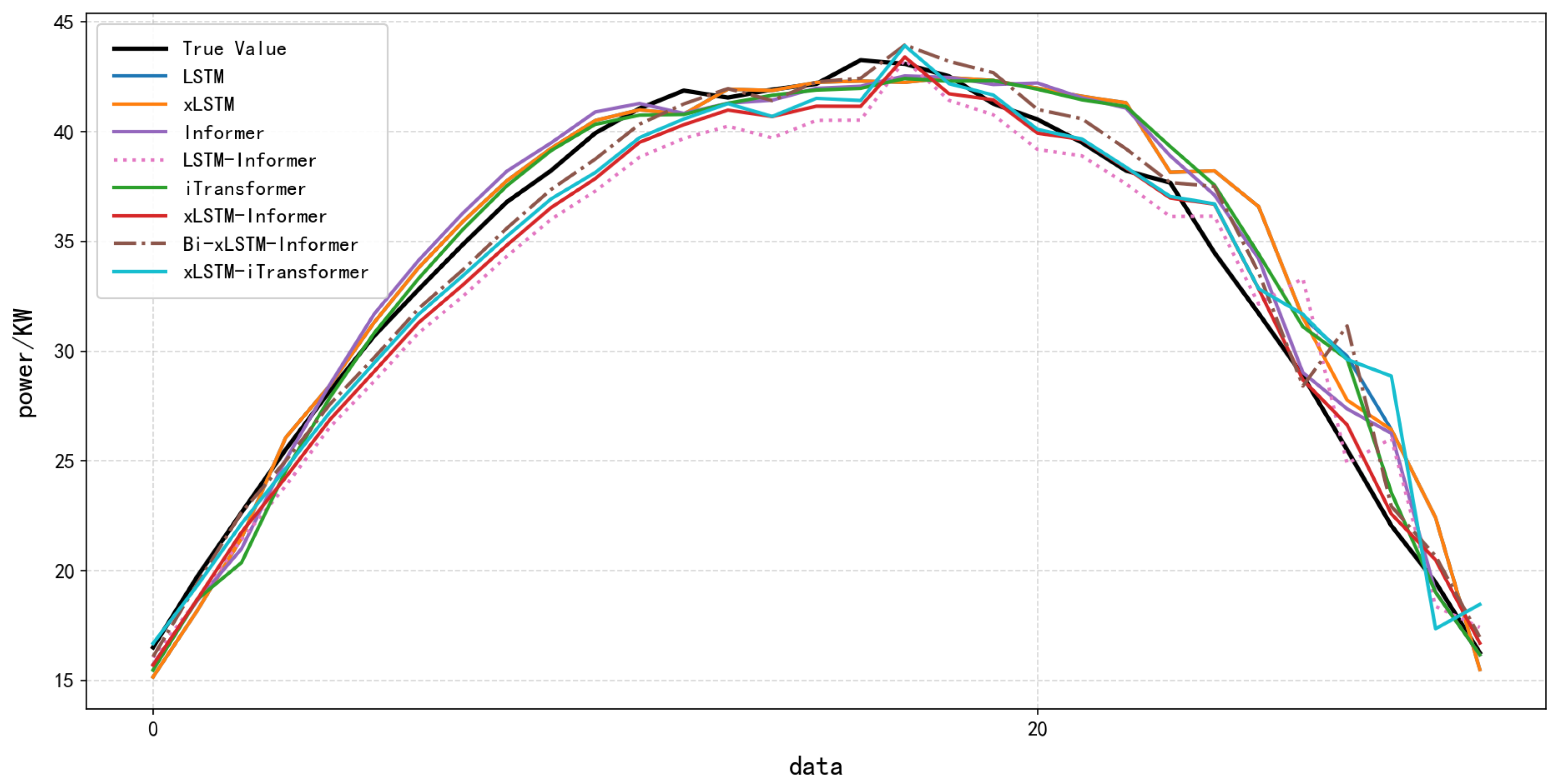
To confirm that the Bi-xLSTM-Informer model can handle PV output variations caused by seasonal changes, experiments were conducted on the extended 2019–2020 dataset (15 min interval).

Table 7. Comparison of Effects of Different Models Based on Full Dataset 2.

Model	R2	MAE	RMSE
LSTM	0.9271	2.7860	3.8920
xLSTM	0.9316	2.7434	3.7707
iTransformer	0.9340	2.6111	3.7048
Informer	0.9354	2.6246	3.6634
LSTM-Informer	0.9477	2.3382	3.2943
xLSTM-iTransformer	0.9577	2.0231	2.9632
xLSTM-Informer	0.9620	1.8943	2.8070
Bi-xLSTM-Informer	0.9678	1.7475	2.5863

presents the prediction performance of the proposed model and benchmark models on the 2020 spring test set, with the training set fixed as the 2019 full-year data.

The results, presented in 7 and Figure 11, demonstrate our proposed Bi-xLSTM-Informer model maintains superior short-term forecasting performance (RMSE: 2.5863, MAE: 1.7475) even when deployed in a future seasonal context (spring 2020)—one with high-frequency, short-interval dynamics not encountered during training. Crucially, it successfully leverages the underlying seasonal patterns learned from the 2019 full-year training data.

The complete training time of the Bi-xLSTM-Informer model is approximately 8 min, with overhead mainly coming from the bidirectional mLSTM and Informer’s ProbSparse attention mechanism. Although its training time is longer than that of the basic LSTM model (5 min), the model offers high prediction accuracy, low error, and strong robustness—meeting the needs of real-time applications. In PV prediction applications, a small improvement in model accuracy can bring significant economic benefits.

In summary, the Bi-xLSTM-Informer hybrid model significantly enhances the overall performance by combining the short-term feature capture capabilities of the bidirectional structure with the Informer’s proficiency in processing long sequences and extracting global information. Specifically, relative to the best baseline model, the proposed model reduces the RMSE by 5.81% and achieves an R² of 98.76%.

6. Conclusions

To improve the accuracy and reliability of short-term PV power forecasting, this study proposed a novel PV forecasting framework that explicitly leverages symmetry principles to enhance accuracy. The method first designs a two-stage feature selection mechanism using Boruta-PCA to effectively extract key features, eliminate multicollinearity interference, and reduce input dimensions. It then constructs a Bi-xLSTM-Informer hybrid model, which combines sequence reversal and feature fusion techniques to form a bidirectional processing layer, integrating the local temporal modeling capabilities of Bi-xLSTM with the global information extraction advantages of Informer. Based on comparisons and validations using public datasets from the Photovoltaic (PV) Power Plant AI Competition, the proposed approach significantly improves prediction accuracy and generalization performance by explicitly embedding symmetry considerations. Experimental results demonstrate that the Bi-xLSTM-Informer model achieves the best prediction performance among all compared models, with an R² of 98.76% and an RMSE of 0.3776. This RMSE value represents a reduction of 5.81% compared to the best-performing benchmark model. It demonstrates excellent stability and adaptability when handling high-dimensional features and complex temporal patterns, along with significant application potential in real-world PV power prediction scenarios.

Future research will explore the transferability of this symmetry-based forecasting framework to multi-energy scenarios such as wind power and hydropower, and will further integrate cutting-edge technologies to enhance the universality, intelligence, and symmetry-aware adaptability of predictions.

References

1. Sun, Y.; Wang, Z.; Wang, J.; Li, Q. Short-Term Solar PV Power Prediction Utilizing the VMD-BKA-BP Neural Network. Symmetry 2025, 17, 784. [Google Scholar] [CrossRef]
2. Mohamad Radzi, P.N.L.; Akhter, M.N.; Mekhilef, S.; Shah, N.M. Review on the Application of PV Forecasting Using Machine Learning for Very Short- to Long-Term Forecasting. Sustainability 2023, 15, 2942. [Google Scholar] [CrossRef]
3. Qiu, Z.; Tian, Y.; Luo, Y.; Gu, T.; Liu, H. Wind and PV Power Generation Forecasting for Virtual Power Plants Based on the Fusion of Improved K-Means Cluster Analysis and Deep Learning. Sustainability 2024, 16, 10740. [Google Scholar] [CrossRef]
4. Alao, A.B.; Adeyanju, O.M.; Chamana, M.; Bayne, S.; Bilbao, A. PV Farm Power Generation Forecast Using PV BatteryModel with Machine Learning Capabilities. Solar 2025, 5, 26. [Google Scholar] [CrossRef]
5. Cervone, G.; Clemente-Harding, L.; Alessandrini, S.; Monache, L.D. Short-term PV power forecasting using Artificial Neural Networks and an Analog Ensemble. Renew. Energy 2017, 108, 274–286. [Google Scholar] [CrossRef]
6. Huang, C.; Yang, M. Memory long and short term time series network for ultra-short-term PV power forecasting. Energy 2023, 279, 127961. [Google Scholar] [CrossRef]
7. Zhang, T.; Zhao, W.; He, Q.; Xu, J. Optimization of Microgrid Dispatching by Integrating PV Power Generation Forecast. Sustainability 2025, 17, 648. [Google Scholar] [CrossRef]
8. de Oliveira Santos, L.; AlSkaif, T.; Barroso, G.C.; de Carvalho, P.C.M. PV power estimation and forecast models integrating physics and machine learning: A review on hybrid techniques. Sol. Energy 2024, 284, 113044. [Google Scholar] [CrossRef]
9. Thaker, J.; Höller, R. Hybrid model for intra-day probabilistic PV power forecast. Renew. Energy 2024, 232, 121057. [Google Scholar] [CrossRef]
10. Patterson, K. An Introduction to ARIMA Models. In Unit Root Tests in Time Series: Key Concepts and Problems; Palgrave Macmillan: London, UK, 2011; pp. 68–122. [Google Scholar]
11. Cao, L.J.N. Support vector machines experts for time series forecasting. Neurocomputing 2003, 51, 321–339. [Google Scholar] [CrossRef]
12. Markovics, D.; Mayer, M.J. Comparison of machine learning methods for PV power forecasting based on numerical weather prediction. Renew. Sustain. Energy Rev. 2022, 161, 112364. [Google Scholar] [CrossRef]
13. Wang, K.; Qi, X.; Liu, H. A comparison of day-ahead PV power forecasting models based on deep learning neural network. Appl. Energy 2019, 251, 113315. [Google Scholar] [CrossRef]
14. Zhou, H.; Zhang, Y.; Yang, L.; Liu, Q.; Yan, K.; Du, Y. Short-Term PV Power Forecasting Based on Long Short Term Memory Neural Network and Attention Mechanism. IEEE Access 2019, 7, 78063–78074. [Google Scholar] [CrossRef]
15. Zhou, X.; Sheil, B.; Suryasentana, S.; Shi, P. Multi-fidelity fusion for soil classification via LSTM and multi-head self-attention CNN model. Adv. Eng. Inform. 2024, 62, 102655. [Google Scholar] [CrossRef]
16. Zhuang, Z.; Wang, H.; Yu, C. Prediction of Short-Term Solar Irradiance Using the ProbSparse Attention Mechanism for a Sustainable Energy Development Strategy. Sustainability 2025, 17, 1075. [Google Scholar] [CrossRef]
17. Das, M.; Arslan, E.; Kaya, S.; Alatas, B.; Akpinar, E.; Özsoy, B. Performance Evaluation of PV Panels in Extreme Environments: A Machine Learning Approach on Horseshoe Island, Antarctica. Sustainability 2025, 17, 174. [Google Scholar] [CrossRef]
18. Ghodbane, M.; El-Amarty, N.; Boumeddane, B.; Hussain, F.; El Fadili, H.; Bennani, S.D.; Akil, M. Improving short-term PV power forecasting with an evolving neural network incorporating time-varying filtering based on empirical mode decomposition. Energy Convers. Manag. 2025, 323, 119261. [Google Scholar] [CrossRef]
19. Lv, Y.; Wang, G.; Huang, S. A short-term load forecasting model based on mixup and transfer learning. Electr. Power Syst. Res. 2022, 207, 107837. [Google Scholar] [CrossRef]
20. Ge, L.; Xian, Y.; Yan, J.; Wang, B.; Wang, Z. A Hybrid Model for Short-term PV Output Forecasting Based on PCA-GWO-GRNN. J. Mod. Power Syst. Clean Energy 2020, 8, 1268–1275. [Google Scholar] [CrossRef]
21. Subbiah, S.S.; Paramasivan, S.K.; Arockiasamy, K.; Senthivel, S.; Thangavel, M. Deep Learning for Wind Speed Forecasting Using Bi-LSTM with Selected Features. Intell. Autom. Soft Comput. 2023, 35, 3829–3844. [Google Scholar] [CrossRef]
22. Kursa, M.B.; Rudnicki, W.R. Feature Selection with the Boruta Package. J. Stat. Softw. 2010, 36, 1–13. [Google Scholar] [CrossRef]
23. Xu, J.; Wei, Y.; Zeng, P. VMD-Based Iterative Boruta Feature Extraction and CNNA-BiLSTM for Short-Term Load Forecasting. Electr. Power Syst. Res. 2025, 238, 111172. [Google Scholar] [CrossRef]
24. Wang, J.; Zhang, Z.; Xu, W.; Li, Y.; Niu, G. Short-Term PV Power Forecasting Using a Bi-LSTM Neural Network Optimized by Hybrid Algorithms. Sustainability 2025, 17, 5277. [Google Scholar] [CrossRef]
25. Kursa, M.B.; Rudnicki, W.R. xLSTM: Extended Long Short-Term Memory. arXiv 2024, arXiv:2405.04517. [Google Scholar] [CrossRef]
26. Kühne, N.L.; Østergaard, J.; Jensen, J.; Tan, Z.-H. xLSTM-SENet: xLSTM for Single-Channel Speech Enhancement. arXiv 2024, arXiv:2501.06146. [Google Scholar] [CrossRef]
27. Zhou, H.Y.; Zhang, S.H.; Peng, J.Q.; Zhang, S.; Li, J.; Xiong, H.; Zhang, W. Informer: Beyond Efficient Transformer for Long Sequence Time-Series Forecasting. Proc. AAAI Conf. Artif. Intell. 2021, 35, 11106–11115. [Google Scholar] [CrossRef]
28. China Industrial Big Data. Big Data Processing and Analysis of AI Operation of PV Station. 13 July 2018. Available online: https://www.datafountain.cn/competitions/303 (accessed on 13 July 2018).
29. Chen, Y.; Xu, J. Solar and Wind Power Data from the Chinese State Grid Renewable Energy Generation Forecasting Competition. Sci. Data 2022, 9, 577. [Google Scholar] [CrossRef] [PubMed]
30. Cao, Y.; Liu, G.; Luo, D.; Bavirisetti, D.P.; Xiao, G. Multi-timescale PV power forecasting using an improved Stacking ensemble algorithm based LSTM-Informer model. Energy 2023, 283, 128669. [Google Scholar] [CrossRef]
31. Zhang, Y.; Kong, L. Photovoltaic Power Prediction Based on Hybrid Modeling of Neural Network and Stochastic Differential Equation. ISA Trans. 2022, 128 Pt B, 181–206. [Google Scholar] [CrossRef]
Figure 1. Structure of the Bi-xLSTM-Informer model.
Symmetry 17 01469 g001
Figure 2. Overall structure of xLSTM.
Symmetry 17 01469 g002
Figure 3. Bi-mLSTM model structure diagram.
Symmetry 17 01469 g003
Figure 4. Structure of Informer model.
Symmetry 17 01469 g004
Figure 5. Flow chart of the experiment.
Symmetry 17 01469 g005
Figure 6. Effectiveness of Boruta’s algorithm.
Symmetry 17 01469 g006
Figure 7. The Effect Diagram of PCA.
Symmetry 17 01469 g007
Figure 8. Model Loss Contrast.
Symmetry 17 01469 g008
Figure 9. Effect of Different Models Based on Full Dataset 1.
Symmetry 17 01469 g009
Figure 10. Different model effects based on sample data.
Symmetry 17 01469 g010
Figure 11. Effect of Different Models Based on Dataset 2.
Symmetry 17 01469 g011