Uniformity Testing and Estimation of Generalized Exponential Uncertainty in Human Health Analytics

Abstract

The entropy function, as a measure of information and uncertainty, has been widely applied in various scientific disciplines. One notable extension of entropy is exponential entropy, which finds applications in fields such as optimization, image segmentation, and fuzzy set theory. In this paper, we explore the continuous case of generalized exponential entropy and analyze its behavior under symmetric and asymmetric probability distributions. Particular emphasis is placed on illustrating the role of symmetry through analytical results and graphical representations, including comparisons of entropy curves for symmetric and skewed distributions. Moreover, we investigate the relationship between the proposed entropy model and other information-theoretic measures such as entropy and extropy. Several non-parametric estimation techniques are studied, and their performance is evaluated using Monte Carlo simulations, highlighting asymptotic properties and the emergence of normality, an aspect closely related to distributional symmetry. Furthermore, the consistency and biases of the estimation methods, which rely on kernel estimation with ${\rho }_{corr}$-mixing dependent data, are presented. Additionally, numerical calculations based on simulation and medical real data are applied. Finally, a test of uniformity using different test statistics is given.

1. Introduction

Entropy is a quantitative measure of a probabilistic system’s information, according to Shannon [1]. He used the probability distribution’s logarithmic function to quantify information. The probability that the $lth$ state of an n-state system will occur is $P{b}_l$, where $0\le P{b}_l\le 1$ and $\sum P{b}_l=1$. $log({\displaystyle \frac{1}{P{b}_l}})$ is the information gain resulting from the appearance of the $lth$ status in such a system, and the system’s entropy is the expected outcome of the gain function. In research pertaining to information theory and its numerous applications, entropy is an essential measure that is well recognized in this field. Therefore, the Shannon entropy function is expressed as

$$\begin{array}{cc}\hfill \Omega \left(Pb\right)& =-\sum _{l=1}^{n}P{b}_{l}log\left(P{b}_l\right).\hfill \end{array}$$

(1)

In discrete circumstances, Shannon entropy is non-negative; however, in continuous cases, it may be negative. The literature on entropy has expanded quickly in order to build information entropy. Renyi [2] entropy, Kapur [3] entropy, Havrda and Charvat [4] entropy, Tsallis [5] entropy, and others are examples of Shannon entropy extensions that have grown in number. More assumptions are required because the knowledge about an event we anticipate falls between finite limits. Pal and Pal [6,7] developed an additional measure, known as exponential entropy among other definitions, parallel to Shannon entropy, based on these considerations following Campbell [8]. Exponential entropy is expressed as

$$\begin{array}{cc}\hfill {\Omega }_{EX}\left(Pb\right)& =\sum _{l=1}^{n}P{b}_l(e^{1-P{b}_l}-1).\hfill \end{array}$$

(2)

Since it appears only reasonable that any measure of information be set to 0 for the degenerative probability distribution $(0,\dots ,0,1,0,\dots ,0)$, the authors have included the $-1$ term. According to them, exponential entropy is superior to Shannon entropy. For instance, Shannon entropy does not have a defined upper bound, although exponential entropy does for the uniform probability distribution $P{b}_l={\displaystyle \frac{1}{n}}$, where $l=1,2,\dots ,n$.

$$\begin{array}{cc}\hfill \underset{n\to \infty }{lim}{\Omega }_{EX}\left({\displaystyle \frac{1}{n}},{\displaystyle \frac{1}{n}},\dots ,{\displaystyle \frac{1}{n}}\right)& =e-1.\hfill \end{array}$$

Additionally, in parallel to Shannon entropy in continuous and discrete situations, Panjehkeh et al. [9] investigated the characteristics and attributes of exponential entropy, including the asymptotic equipartition property, chain rule, the subadditivity, and invariancy under monotone transformation. They introduced continuous exponential entropy by

$$\begin{array}{cc}\hfill C{\Omega }_{EX}\left(Y\right)& ={\int }_{R}g\left(y\right)\left(e^{1-g\left(y\right)}\right)dy,\hfill \end{array}$$

(3)

where Y is a continuous random variable with the probability density function (PDF) g and support R, and we can see that Panjehkeh et al. [9] removed the term $-1$ from their measure to make it always non-negative against Shannon entropy. Building on the exponential entropy of Equation (2), Kvalseth [10] introduced a more general form, which is referred to as generalized exponential entropy by

$$\begin{array}{cc}\hfill {\Omega }_{GEX}\left(Pb\right)& ={\displaystyle \frac{1}{\eta }}\sum _{l=1}^{n}P{b}_l(e^{1-P{b}_l^{\eta }}-1),\hfill \end{array}$$

(4)

where the parameter $\eta$ is arbitrary and has a non-zero real value (i.e., $\eta \in \mathbb{R}\setminus \left\{0\right\}$).

Another measure that has been used in many research studies is the dual of Shannon entropy, also known as extropy, which is presented by Lad et al. [11] as

$$D\Omega \left(Pb\right)=-\sum _{l=1}^n(1-P{b}_l)log(1-P{b}_l).$$

(5)

Lad et al. [11] expanded the function $(1-P{b}_l)log(1-P{b}_l)$ to about $-P{b}_l+{\displaystyle \frac{1}{2}}P{b}_l^2$ for small values of $P{b}_l$ based on the expansion of the Maclaurin series. $D\Omega \left(Pb\right)$ may therefore be roughly represented as $1-{\displaystyle \frac{1}{2}}{\sum }_{l=1}^{n}P{b}_l^2$, where $l=1,2,\dots ,n$, for tiny maximum values of $P{b}_l$. Let us also define $g\left(y_l\right)\equiv {\displaystyle \frac{P{b}_l}{\Delta y}}$, where $\Delta y\equiv {\displaystyle \frac{(y_n-y_1)}{(n-1)}}$ for every given n. Therefore, the approximation $D\Omega \left(Pb\right)\approx 1-{\displaystyle \frac{\Delta y}{2}}{\sum }_{l=1}^{n}g{\left(y_l\right)}^2\Delta y$ represents a simple scale and location transformation of $-{\displaystyle \frac{1}{2}}{\sum }_{l=1}^{n}g{\left(y_l\right)}^2\Delta y$. Thus, the differential extropy measure of the density, g, was defined by Lad et al. [11] as

$$D\Omega \left(Y\right)=D\Omega \left(g\right)=-{\displaystyle \frac{1}{2}}{\int }_{-\infty }^{\infty }{g}^2\left(y\right)dy=\underset{\Delta y⟶0}{lim}\left[{\displaystyle \frac{D\Omega \left(Pb\right)-1}{\Delta y}}\right].$$

(6)

Non-parametric techniques for estimating information techniques have been presented by several scholars. Vasicek [12] proved his entropy estimator in situations where the measure depends on the PDF by making use of the capability to represent the continuous case of Equation (1) in a different way as

$$C\Omega \left(Y\right)=-{\int }_0^{\infty }g\left(y\right)logg\left(y\right)dy=-{\int }_0^{1}log{\left[{\displaystyle \frac{d}{d\xi }}{G}^{-1}\left(\xi \right)\right]}^{-1}d\xi ,$$

(7)

noting that $G\left(y\right)$ is the cumulative distribution function (CDF). The difference operator was then used in place of the CDF, G, and the empirical CDF, $G_n$, was used in place of the differential operator function. The derivative of $G^{-1}\left(\xi \right)$ was then estimated using the function of the order statistics. Formally speaking, Vasicek’s estimator is written as follows given the order statistic $Y_{(1;n)}\le \dots \le Y_{(n;n)}$ from the sample chosen at random $Y_1,\dots ,Y_n$ by:

$$C\Omega \left(G_n\right)={\displaystyle \frac{1}{n}}\sum _{t=1}^{n}log\left[{\displaystyle \frac{n}{2\lambda }}(Y_{(t+\lambda ;n)}-Y_{(t-\lambda ;n)})\right],$$

(8)

where $\lambda <{\displaystyle \frac{n}{2}}$ is the positive aspects integer panel size, $Y_{(t;n)}=Y_{(1;n)}$ if $t<1$, and $Y_{(t;n)}=Y_{(n;n)}$ if $t>n$. The limitations of (8) at its limits are then pointed out by Ebrahimi et al. [13], who then modify it to propose their entropy estimator as

$$C\Omega \left(G_n\right)={\displaystyle \frac{1}{n}}\sum _{t=1}^{n}log\left[{\displaystyle \frac{n}{{\Xi }_t\lambda }}(Y_{(t+\lambda ;n)}-Y_{(t-\lambda ;n)})\right],$$

(9)

noting that

$${\Xi }_t=\left\{\begin{array}{cc}1+{\displaystyle \frac{t-1}{\lambda }},\hfill & \hfill 1\le t\le \lambda \\ 2,\hfill & \hfill \lambda +1\le t\le n-\lambda \\ 1+{\displaystyle \frac{n-t}{\lambda }},\hfill & \hfill n-\lambda +1\le t\le n.\end{array}\right.$$

(10)

It should be noted that Vasicek’s entropy estimator is used in most of the experiments described above because of its ease of use and particularly high relative accuracy. For example, Qiu and Jia [14] and Noughabi and Jarrahiferiz [15] used the approach that was described to estimate the extropy measure. Additionally, Wachowiak et al. [16] estimated generalized entropies such as the Tsallis and Renyi entropies using sample spacing. Sakr and Mohamed [17] used kernel function, local linear model, and spacing to give a number of non-parametric estimation methods for the Sharma–Taneja–Mittal entropy measurement of a random variable that is continuous with known support. Moreover, the cumulative residual generalized exponential entropy measure was proposed by Sakr and Mohamed [18] using several non-parametric estimating techniques.

Under the mixing coefficients ${\alpha }_{corr}$-mixing, ${\varphi }_{corr}$-mixing, and ${\rho }_{corr}$-mixing, which are described by Rosenblatt [19], Ibragimov [20], and Kolmogorov and Rozanov [21], another kind of non-parametric estimation relies on the kernel density estimator. Bradley [22] spoke about the kernel density estimator’s asymptotic normality and poor consistency under ${\rho }_{corr}$-mixing. In the context of ${\alpha }_{corr}$-mixing, Masry [23] developed a non-parametric recursive density estimator and examined a few of its characteristics. The local linear estimate of the residual entropy function of conditional distributions, whose underlying data are assumed to be ${\rho }_{corr}$-mixing, was covered by Rajesh et al. [24]. The kernel estimate of cumulative residual Tsallis entropy and its dynamic variant under ${\rho }_{corr}$-mixing-dependent data was introduced by Irshad et al. [25].

Work Motivation

Building upon existing research on entropy measures involving exponential functions and their generalizations, it is evident that focusing solely on the discrete case provides an incomplete perspective without a parallel investigation of the continuous case. As previously noted, exponential entropy in discrete settings has been extensively explored across multiple disciplines, for instance, see the works of Ye and Cui [26] and Wang et al. [27]. Consequently, it becomes necessary to extend this exploration to the continuous domain, particularly by elucidating the applications where continuous formulations are relevant. An additional point of interest is the foundational role of the exponential function in the proposed model. It prompts the question: can this functional form address specific challenges related to uncertainty?

Among the various probability distributions, the uniform distribution stands out for its simplicity and utility. It allocates equal likelihood to all outcomes within a specified interval in the continuous setting, making it an ideal benchmark for comparison. Its practical relevance is seen in areas such as random number generation. In the field of economics, for example, patterns of supply and demand often deviate from the traditional normal distribution, prompting the need for alternative models that better reflect observed behaviors. Wanke [28] highlights the effectiveness of the uniform distribution in estimating lead times for inventory control, especially during the initial evaluation phase of a new product. Furthermore, social scientists often adopt the uniform distribution to represent ignorance or lack of prior knowledge, such as when employing simulations in which the actual distribution is unknown. In measurement cases, the uniform model is also used to characterize errors from certain instruments. These diverse applications underline the importance of designing hypothesis tests that are both straightforward and computationally efficient for assessing whether a dataset follows a uniform distribution. As such, a comprehensive discussion on uniformity testing is both necessary and timely.

In addition to this modeling perspective, our work addresses a gap in the literature by comparing multiple estimation techniques for generalized exponential entropy. While entropy-based measures have gained popularity, relative studies have examined how different estimators affect the accuracy and performance of entropy-based models in both theoretical and applied settings. Therefore, we introduce and compare four distinct estimators, investigate their asymptotic properties, and evaluate their practical performance through simulations and real data applications. This comparative approach enhances the interpretability and robustness of entropy-based statistical inference.

This suggestion aims to present the concept of generalized exponential entropy in the continuous domain and discuss its properties with various applications, including the test of uniformity. The structure of this study is organized as follows. Section 2 presents the continuous case of generalized exponential entropy, including applications to some well-known distributions. Furthermore, the relationship between the proposed model and entropy and extropy measures is discussed. In Section 3, various procedures for the non-parametric estimation of generalized exponential entropy are investigated. Moreover, the characteristics and consistency of kernel density estimation with ${\rho }_{corr}$-mixing dependent data are analyzed for generalized exponential entropy. Section 4 applies numerical calculations of the obtained estimators to simulations and real-world medical data. Finally, testing for uniformity using the proposed statistics, along with a power comparison, is conducted in Section 5.

2. Generalized Exponential Entropy and Its Complementary Dual

In this section, we will present the continuous case of generalized exponential entropy. In parallel to the discrete case in (4), let Y be a continuous random variable with PDF g, and continuous generalized exponential entropy can be presented by

$$\begin{array}{cc}\hfill C{\Omega }_{GEX}\left(Y\right)& ={\displaystyle \frac{1}{\eta }}{\int }_{-\infty }^{\infty }g\left(y\right)(e^{1-g^{\eta }\left(y\right)}-1)dy\hfill \\ & ={\displaystyle \frac{1}{\eta }}\left({\int }_{-\infty }^{\infty }g\left(y\right)e^{1-g^{\eta }\left(y\right)}dy-1\right),\hfill \end{array}$$

(11)

where $\eta \in \mathbb{R}\setminus \left\{0\right\}$.

Example 1.

With PDF $g\left(y\right)=\gamma e^{-\gamma y}$, $\gamma >0$, let us assume that the continuously distributed random variable Y follows an exponential distribution symbolized by $EXP\left(\gamma \right)$. The continuous generalized exponential entropy is therefore obtained from (11) by

$$\begin{array}{cc}\hfill C{\Omega }_{GEX}\left(Y\right)& ={\displaystyle \frac{-1+\frac{e{\left({\gamma }^{\eta }\right)}^{-1/\eta }\left(\Gamma \left(\frac{1}{\eta }\right)-I\Gamma \left(\frac{1}{\eta };{\gamma }^{\eta }\right)\right)}{\eta }}{\eta }},\hfill \end{array}$$

(12)

where $0\ne \eta \in \mathbb{R}$, $\Gamma (.)$ is the Euler gamma function, and $I\Gamma (.;.)$ is the incomplete gamma function.

Figure 1 shows the generalized exponential entropy of exponential distribution with $\gamma =0.5,1,1.5,2$. Although the parameter $\eta$ does not equal zero, Figure 1 reveals a near-symmetric pattern of the generalized exponential entropy around $\eta =0$. This visual symmetry suggests a balanced response of the entropy measure to variations in $\eta$ on both sides of the origin. Such behavior highlights the structural regularity of the proposed measure and offers useful insights when analyzing distributions that exhibit or deviate from symmetry.

Example 2.

With PDF $g\left(y\right)={\displaystyle \frac{1}{{\varphi }_2-{\varphi }_1}}$, $-\infty <a<b<\infty$, let us assume that the continuously distributed random variable Y follows a uniform distribution represented by $U({\varphi }_1,{\varphi }_2)$. The continuous generalized exponential entropy is therefore obtained from (11) by

$$C{\Omega }_{GEX}\left(Y\right)={\displaystyle \frac{-1+e^{1-{\left(\frac{1}{{\varphi }_2-{\varphi }_1}\right)}^{\eta }}}{\eta }},$$

(13)

where $0\ne \eta \in \mathbb{R}$. Specifically, the generalized exponential entropy becomes zero when the difference between ${\varphi }_1$ and ${\varphi }_2$ is precisely one.

The generalized exponential entropy when $\eta$ goes to 0 is discussed in the following assertion.

Proposition 1.

With PDF $g\left(y\right)$, assuming that Y is a continual random variable. When η goes to zero, the continuous generalized exponential entropy then follows the continuous Shannon entropy from (11), i.e.,

$$\underset{\eta \to 0}{lim}C{\Omega }_{GEX}\left(Y\right)=C\Omega \left(Y\right),$$

where $0\ne \eta \in \mathbb{R}$, and $C\Omega \left(Y\right)$ is defined in (7).

Proof. 

Applying $L^{\prime }H\widehat{o}pita{l}^{\prime }s$ rule to (11), we obtain

$$\begin{array}{cc}\hfill \underset{\eta \to 0}{lim}C{\Omega }_{GEX}\left(Y\right)& =\underset{\eta \to 0}{lim}{\displaystyle \frac{1}{\eta }}\left({\int }_{-\infty }^{\infty }g\left(y\right)e^{1-g^{\eta }\left(y\right)}dy-1\right)\hfill \\ & =\underset{\eta \to 0}{lim}\left({\int }_{-\infty }^{\infty }-e^{1-g^{\eta }\left(y\right)}{g}^{1+\eta }\left(y\right)log\left(g\left(y\right)\right)dy\right)\hfill \\ & =-\left({\int }_{-\infty }^{\infty }g\left(y\right)log\left(g\left(y\right)\right)dy\right)\hfill \\ & =C\Omega \left(Y\right).\hfill \end{array}$$

 □

Proposition 2.

In order for Y and Z to be absolutely random variables that are continuous, let $Z=\Psi \left(Y\right)$, where Ψ is a precisely increasing function and $|{\Psi }^{\prime }\left(y\right)|\le 1$. Next,

$$C{\Omega }_{GEX}(\Psi \left(Y\right))\le C{\Omega }_{GEX}\left(Y\right),$$

and when $|{\Psi }^{\prime }\left(y\right)|=1$, equality is maintained.

Proof. 

Utilizing Equation (11), and let $Z=\Psi \left(Y\right)$, then we have

$$\begin{array}{cc}\hfill C{\Omega }_{GEX}\left(Z\right)& ={\displaystyle \frac{1}{\eta }}\left({\int }_{-\infty }^{\infty }g\left({\Psi }^{-1}\left(z\right)\right){\displaystyle \frac{1}{|{\Psi }^{\prime }\left({\Psi }^{-1}\left(z\right)\right)|}}{e}^{1-{\left(g\left({\Psi }^{-1}\left(z\right)\right){\displaystyle \frac{1}{|{\Psi }^{\prime }\left({\Psi }^{-1}\left(z\right)\right)|}}\right)}^{\eta }}dy-1\right).\hfill \end{array}$$

Assume that $\Psi$ is strictly growing. When $z=\Psi \left(y\right)$ is set, we get

$$\begin{array}{cc}\hfill C{\Omega }_{GEX}\left(Z\right)& ={\displaystyle \frac{1}{\eta }}\left({\int }_{{\Psi }^{-1}(-\infty )}^{{\Psi }^{-1}(\infty )}g\left(y\right)e^{1-{\left(g\left(y\right){\displaystyle \frac{1}{{\Psi }^{\prime }\left(y\right)}}\right)}^{\eta }}dy-1\right)\hfill \\ & \le {\displaystyle \frac{1}{\eta }}\left({\int }_{-\infty }^{\infty }g\left(y\right)e^{1-g^{\eta }\left(y\right)}dy-1\right)=C{\Omega }_{GEX}\left(Y\right).\hfill \end{array}$$

 □

Complementary Dual of Generalized Exponential Entropy

In this subsection, we will discuss the complementary dual of generalized exponential entropy and its relation to the extropy measure. Inspired by the extropy measure introduced by Lad et al. [11] in the discrete case, as given in (5), we can obtain the complementary dual of generalized exponential entropy by replacing $P{b}_l$ with $1-P{b}_l$ in (4), $l=1,2,\dots ,n$, as follows

$$\begin{array}{cc}\hfill D{\Omega }_{GEX}\left(Pb\right)& ={\displaystyle \frac{1}{\eta }}\sum _{l=1}^n(1-P{b}_l)(e^{1-{(1-P{b}_l)}^{\eta }}-1).\hfill \end{array}$$

(14)

We can expanded the function $(1-P{b}_l)(e^{1-{(1-P{b}_l)}^{\eta }}-1)$ for small values of $P{b}_l$ based on the expansion of the Maclaurin series. For $|P{b}_l|<1$, the binomial expansion for $1-{(1-P{b}_l)}^{\eta }$ is:

$$1-{(1-P{b}_l)}^{\eta }=\eta P{b}_l-{\displaystyle \frac{\eta (\eta -1)}{2}}P{b}_l^2+\mathcal{O}\left(P{b}_l^3\right).$$

Substitute $1-{(1-P{b}_l)}^{\eta }$ into the exponential function. Recall the Maclaurin series for $e^z$:

$$e^z=1+z+{\displaystyle \frac{z^2}{2}}+{\displaystyle \frac{z^3}{6}}+\mathcal{O}\left(z^4\right).$$

Here, $z=1-{(1-P{b}_l)}^{\eta }$, which we approximated as:

$$z=\eta P{b}_l-{\displaystyle \frac{\eta (\eta -1)}{2}}P{b}_l^2+\mathcal{O}\left(P{b}_l^3\right).$$

Now substitute into the exponential series:

$$e^{1-{(1-P{b}_l)}^{\eta }}=1+\left(\eta P{b}_l-{\displaystyle \frac{\eta (\eta -1)}{2}}P{b}_l^2\right)+{\displaystyle \frac{1}{2}}{\left(\eta P{b}_l\right)}^2+\mathcal{O}\left(P{b}_l^3\right).$$

Simplify:

$$e^{1-{(1-P{b}_l)}^{\eta }}-1=\eta P{b}_l+\left(-{\displaystyle \frac{\eta (\eta -1)}{2}}+{\displaystyle \frac{{\eta }^2}{2}}\right)P{b}_l^2+\mathcal{O}\left(P{b}_l^3\right).$$

Thus:

$$e^{1-{(1-P{b}_l)}^{\eta }}-1=\eta P{b}_l+{\displaystyle \frac{\eta }{2}}P{b}_l^2+\mathcal{O}\left(P{b}_l^3\right).$$

(15)

Multiply (15) by $1-P{b}_l$, and after simple calculations we get

$$(1-P{b}_l)\left(e^{1-{(1-P{b}_l)}^{\eta }}-1\right)=\eta P{b}_l-{\displaystyle \frac{\eta }{2}}P{b}_l^2+\mathcal{O}\left(P{b}_l^3\right).$$

(16)

Therefore, $D{\Omega }_{GEX}\left(Pb\right)$ may therefore be roughly represented as $1-{\displaystyle \frac{1}{2}}{\sum }_{l=1}^{n}P{b}_l^2$, where $l=1,2,\dots ,n$, for tiny maximum values of $P{b}_l$. Let us also define $g\left(y_l\right)\equiv {\displaystyle \frac{P{b}_l}{\Delta y}}$, where $\Delta y\equiv {\displaystyle \frac{(y_n-y_1)}{(n-1)}}$ for every given n. Therefore, the approximation $D{\Omega }_{GEX}\left(Pb\right)\approx 1-{\displaystyle \frac{\Delta y}{2}}{\sum }_{l=1}^{n}g{\left(y_l\right)}^2\Delta y$ represents a simple scale and location transformation of $-{\displaystyle \frac{1}{2}}{\sum }_{l=1}^{n}g{\left(y_l\right)}^2\Delta y$. Then, we see that

$$D{\Omega }_{GEX}\left(Y\right)\equiv -{\displaystyle \frac{1}{2}}{\int }_{-\infty }^{\infty }{g}^2\left(y\right)dy=\underset{\Delta y⟶0}{lim}\left[{\displaystyle \frac{D{\Omega }_{GEX}\left(Pb\right)}{\Delta y}}\right].$$

Thus, we can see that the complementary dual of generalized exponential entropy can be approximated as the differential extropy measure of the density, g, which is defined by Lad et al. [11]. Meanwhile, for the complete differential complementary dual of generalized exponential entropy and entropy given, respectively, by

$$D{\Omega }_{GEX}\left(Y\right)={\displaystyle \frac{1}{\eta }}{\int }_{-\infty }^{\infty }(1-g\left(y\right))(e^{1-{(1-g\left(y\right))}^{\eta }}-1)dy,$$

(17)

$$D\Omega \left(Y\right)=-{\int }_{-\infty }^{\infty }(1-g\left(y\right))log(1-g\left(y\right))dy,$$

(18)

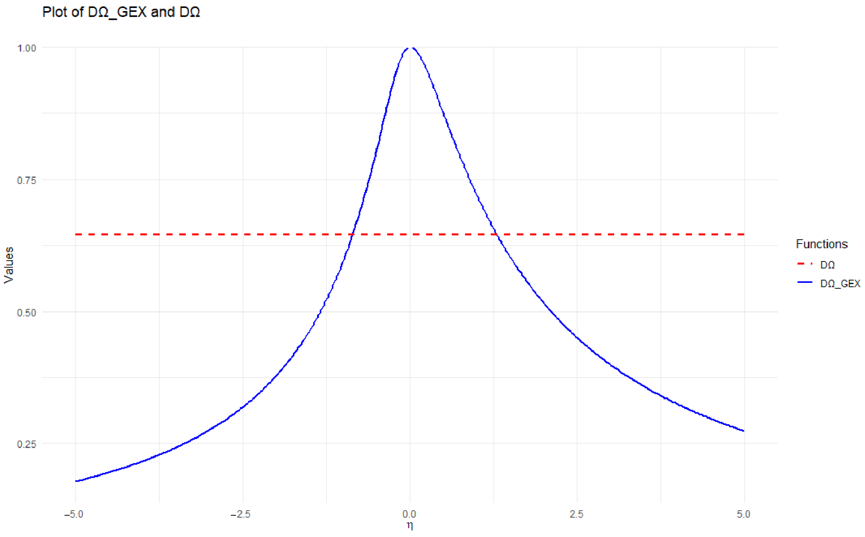
we will discuss their behaviour using the following example. Under the $EXP\left(1\right)$ distribution, Figure 2 shows the plots of (17) and (18), and we can see that $D{\Omega }_{GEX}\left(Y\right)$ is equal to $D\Omega \left(Y\right)$ when $\eta =1.295626$, and $-0.86261$.

3. Proposed Estimation Procedures

Here we provide a number of non-parametric estimation techniques for generalized exponential entropy and compare their performance with some of the leading alternatives, assuming that $Y_{(1;n)}\le \dots \le Y_{(n;n)}$ indicate ordering statistics obtained from a sample with a random size of n taken from an undefined continuous CDF, G, and that follows the PDF g.

3.1. First Technique

By the same manner of Vasicek’s estimator given in (8) to estimate the entropy function, we can suppose the estimator of generalized exponential entropy as follows

$$C_1{\Omega }_{GEX}\left(G_n\right)={\displaystyle \frac{1}{\eta }}\left[{\displaystyle \frac{1}{n}}\sum _{t=1}^n{e}^{1-{\left({\displaystyle \frac{2\lambda }{n(Y_{(t+\lambda ;n)}-Y_{(t-\lambda ;n)})}}\right)}^{\eta }}-1\right],$$

(19)

where $0\ne \eta \in \mathbb{R}$, $\lambda <{\displaystyle \frac{n}{2}}$ is the positive aspects integer panel size, $Y_{(t;n)}=Y_{(1;n)}$ if $t<1$, and $Y_{(t;n)}=Y_{(n;n)}$ if $t>n$.

We will then use Monte Carlo simulation to talk about asymptotic normalcy. Our goal is to confirm that:

$${\Delta }_1={\displaystyle \frac{C_1{\Omega }_{GEX}\left(G_n\right)-E\left[C_1{\Omega }_{GEX}\left(G_n\right)\right]}{\sqrt{Var\left[C_1{\Omega }_{GEX}\left(G_n\right)\right]}}},$$

exhibits a standard distribution that is normal. With a parameter of 1, an $EXP\left(1\right)$ distribution with $\eta =2$ and $\eta =3$ yields 1000 samples, each with a size of $n=50$ and $n=100$. The histograms in Figure 3 and Figure 4 are used to confirm that the estimators in (19) are asymptotically normal.

3.2. Second Technique

We may assume the estimator of generalized exponential entropy in the same way as the Ebrahimi et al. [13] estimator provided in (9) to estimate the entropy function as follows

$$C_2{\Omega }_{GEX}\left(G_n\right)={\displaystyle \frac{1}{\eta }}\left[{\displaystyle \frac{1}{n}}\sum _{t=1}^n{e}^{1-{\left({\displaystyle \frac{{\Xi }_t\lambda }{n(Y_{(t+\lambda ;n)}-Y_{(t-\lambda ;n)})}}\right)}^{\eta }}-1\right],$$

(20)

where $0\ne \eta \in \mathbb{R}$, $\lambda <{\displaystyle \frac{n}{2}}$ is the positive aspects integer panel size, $Y_{(t;n)}=Y_{(1;n)}$ if $t<1$, and $Y_{(t;n)}=Y_{(n;n)}$ if $t>n$, and ${\Xi }_t$ is defined in (10).

We will then use Monte Carlo simulation to talk about asymptotic normalcy. Our goal is to confirm that:

$${\Delta }_2={\displaystyle \frac{C_2{\Omega }_{GEX}\left(G_n\right)-E\left[C_2{\Omega }_{GEX}\left(G_n\right)\right]}{\sqrt{Var\left[C_2{\Omega }_{GEX}\left(G_n\right)\right]}}},$$

exhibits a standard distribution that is normal. With a parameter of 1, an $EXP\left(1\right)$ distribution with $\eta =2$ and $\eta =3$ yields 1000 samples, each with a size of $n=50$ and $n=100$. The histograms in Figure 5 and Figure 6 are used to confirm that the estimators in (20) are asymptotically normal.

3.3. Third Technique

The recommended estimator is presented in the following way based on a local linear frame. Consider the sample data that have been supplied. $(K_n\left(Y_{(1;n)}\right),Y_{(1;n)})$, $(K_n\left(Y_{(2;n)}\right),Y_{(2;n)})$,…, $(K_n\left(Y_{(n;n)}\right),Y_{(n;n)})$. The estimator $C_1{\Omega }_{GEX}\left(G_n\right)$ from (19) may be expressed as

$$C_1{\Omega }_{GEX}\left(G_n\right)={\displaystyle \frac{1}{\eta }}\left[{\displaystyle \frac{1}{n}}\sum _{t=1}^n{e}^{1-{\left[{\displaystyle \frac{\left(\frac{t+\lambda }{n}\right)-\left(\frac{t-\lambda }{n}\right)}{\left(Y_{(t+\lambda ;n)}-Y_{(t-\lambda ;n)}\right)}}\right]}^{\eta }}-1\right],$$

where $\left[{\displaystyle \frac{\left(\frac{t+\lambda }{n}\right)-\left(\frac{t-\lambda }{n}\right)}{\left(Y_{(t+\lambda ;n)}-Y_{(t-\lambda ;n)}\right)}}\right]$ is the straight slope line of the points $(K_n\left(Y_{(t+\lambda ;n)}\right),Y_{(t+\lambda ;n)})$ and $(K_n\left(Y_{(t-\lambda ;n)}\right),Y_{(t-\lambda ;n)})$. Consequently, the generalized exponential entropy estimator derived from the least squares approach is given by

$$\begin{array}{cc}\hfill C_3{\Omega }_{GEX}\left(G_n\right)& ={\displaystyle \frac{1}{n}}\left[{\displaystyle \frac{1}{n}}\sum _{t=1}^n{e}^{1-{\left[{\displaystyle \frac{{\sum }_{j=t-\lambda }^{t+\lambda }(Y_{(j;n)}-{\overline{Y}}_{(t;n)})(j-t)}{n{\sum }_{j=t-\lambda }^{t+\lambda }{\left(Y_{(j;n)}-{\overline{Y}}_{(t;n)}\right)}^2}}\right]}^{\eta }}-1\right],\hfill \end{array}$$

(21)

where ${\overline{Y}}_{(t;n)}={\displaystyle \frac{1}{2\lambda +1}}{\sum }_{j=t-\lambda }^{t+\lambda }{Y}_{(j;n)}$, and the approach is achieved comparable to that described by Correa [29] to estimate Shannon entropy. Additionally, this approach employed the local linear model under the points $2\lambda +1$ as

$$K\left(y_{(j;n)}\right)={\theta }_1+{\theta }_2{y}_{(j;n)}+error,j=\lambda -t,\dots ,\lambda +t.$$

We will then use Monte Carlo simulation to talk about asymptotic normalcy. Our goal is to confirm that:

$${\Delta }_3={\displaystyle \frac{C_3{\Omega }_{GEX}\left(G_n\right)-E\left[C_3{\Omega }_{GEX}\left(G_n\right)\right]}{\sqrt{Var\left[C_3{\Omega }_{GEX}\left(G_n\right)\right]}}},$$

exhibits a standard distribution that is normal. With a parameter of 1, an $EXP\left(1\right)$ distribution with $\eta =2$ and $\eta =3$ yields 1000 samples, each with a size of $n=50$ and $n=100$. The histograms in Figure 7 and Figure 8 are used to confirm that the estimators in (21) are asymptotically normal.

3.4. Fourth Technique

Assuming that the underlying lifetimes are ${\rho }_{corr}$-mixing, we will address the non-parametric estimate of generalized exponential entropy using the kernel kind estimation in this subsection. In the following, we present the concept of ${\rho }_{corr}$-mixing (as discussed in Kolmogorov and Rozanov [21]).

Definition 1.

For a probability space $(Ws,\mathcal{Fs},Ps)$, let ${\mathcal{Fs}}_i^t$ be the Σ-algebra of events produced by the random variables $\{Y_k:i\le k\le t\}$. Asymptotically uncorrelated is the state of the stationary process $\left\{Y_k\right\}$ if

$$\underset{M\in J_2\left({\mathcal{F}}_i^{-\infty }\right),N\in J_2\left({\mathcal{F}}_{i+t}^{+\infty }\right)}{sup}{\displaystyle \frac{\left|\mathit{cov}\right(M,N\left)\right|}{\sqrt{\mathit{var}\left(M\right)\mathit{var}\left(N\right)}}}={\rho }_{corr}\left(t\right)\to 0,$$

as $t\to +\infty$, where ${\rho }_{corr}\left(t\right)$ is the maximum value of the coefficient of correlation or the ${\rho }_{corr}$-mixing coefficient, and $J_2\left({\mathcal{F}}_a^b\right)$ indicates all collection of second-order measurable variables to be random with regard to ${\mathcal{F}}_a^b$.

Consider the strictly stable process ${\left\{Y_t\right\}}_{t=1}^n$, which has a univariate PDF $g\left(y\right)$. The lifetimes are considered to be ${\rho }_{corr}$-mixing, meaning that $Y_t$s do not necessarily need to be mutually independent. A recursive density estimator of $g\left(y\right)$ was presented by Wegman and Davies [30] and is provided by (see also, Parzen [31])

$$\begin{array}{cc}\hfill {\widehat{g}}^{*}\left(Y_r\right)& ={\displaystyle \frac{1}{n\sqrt{{\beta }_n}}}\sum _{t=1}^n{\displaystyle \frac{1}{\sqrt{{\beta }_t}}}\Lambda \left({\displaystyle \frac{Y_r-Y_t}{{\beta }_t}}\right),r=1,\dots ,n,\hfill \end{array}$$

(22)

Suppose $\Lambda \left(y\right)$ meet the requirements listed below:

• $sup|\Lambda (y\left)\right|<+\infty ;$
• ${\int }_{-\infty }^{+\infty }|\Lambda \left(y\right)|dy<+\infty ;$
• ${lim}_{\left|y\right|\to +\infty }|y\Lambda \left(y\right)|=0;$
• ${\int }_{-\infty }^{+\infty }\Lambda \left(y\right)dy=1.$

${\beta }_n\to 0$ and $n{\beta }_n\to +\infty$ are satisfied by the bandwidth parameter ${\beta }_n$ as $n\to +\infty$. Let y be a location where g continues. Provided that the continuously differentiable $(t+1)$-times as g at location y which we have:

$$\underset{v}{sup}|f^{(t+1)}\left(v\right)|=Q<+\infty .$$

Suppose that:

$${\int }_{-\infty }^{+\infty }{\left|v\right|}^k|\Lambda \left(v\right)|dv<+\infty ,k=1,2,\dots ,t+1.$$

Furthermore, the bandwidth parameter to be used, ${\beta }_n$, fulfills:

$${\displaystyle \frac{1}{n}}\sum _{l=1}^n{\left({\displaystyle \frac{{\beta }_l}{{\beta }_n}}\right)}^{j+{\displaystyle \frac{1}{2}}}\to {\mathbb{B}}_{j+{\displaystyle \frac{1}{2}}}<+\infty ,\mathrm{as}n\to +\infty ,j=0,1,2,\dots ,t+1.$$

Next, as stated by Masry [23], the mean and variance of ${\widehat{g}}^{*}\left(y\right)$ are as follows:

$$\mathbb{E}\left({\widehat{g}}^{*}\left(y\right)\right)\simeq {\mathbb{B}}_{0.5}\left(g\left(y\right)+{\displaystyle \frac{{\beta }_n^2{d}_2}{2{\mathbb{B}}_{0.5}}}{g}^{\left(2\right)}\left(y\right){\mathbb{B}}_{2.5}\right),$$

(23)

and:

$$\mathrm{Var}\left({\widehat{g}}^{*}\left(y\right)\right)\simeq {\displaystyle \frac{g\left(y\right)}{n{\beta }_n}}{D}_2,$$

where

$$d_2={\int }_{-\infty }^{+\infty }{v}^2\Lambda \left(v\right)dv\mathrm{and}{D}_2={\int }_{-\infty }^{+\infty }{\Lambda }^2\left(v\right)dv,$$

and $g^{\left(2\right)}\left(y\right)$ is the $2nd$ derivative of g regarding y. ${\widehat{g}}^{*}\left(y\right)$ does not constitute an asymptotically unbiased estimation of $g\left(y\right)$, according to Equation (23). An asymptotically unbiased estimate of $g\left(y\right)$ may be found via simple scaling on (22) and is provided by:

$$\begin{array}{cc}\hfill \widehat{g}\left(y\right)& ={\displaystyle \frac{{\widehat{g}}^{*}\left(y\right)}{{\mathbb{B}}_{0.5}}}\hfill \\ & ={\displaystyle \frac{1}{n{\mathbb{B}}_{0.5}\sqrt{{\beta }_n}}}\sum _{t=1}^n{\displaystyle \frac{1}{\sqrt{{\beta }_t}}}\Lambda \left({\displaystyle \frac{y-Y_t}{{\beta }_t}}\right)\hfill \end{array}$$

(24)

According to Masry [23], the bias and variance of $\widehat{g}\left(y\right)$ are as follows:

$$\mathrm{Bias}\left(\widehat{g}\left(y\right)\right)\simeq {\displaystyle \frac{{\beta }_n^2{d}_2}{2{\mathbb{B}}_{0.5}}}{g}^{\left(2\right)}\left(y\right){\mathbb{B}}_{2.5},$$

(25)

and

$$\mathrm{Var}\left(\widehat{g}\left(y\right)\right)\simeq {\displaystyle \frac{g\left(y\right)}{n{\beta }_n{\mathbb{B}}_{0.5}^2}}{D}_2.$$

(26)

Since generalized exponential entropy can be written as

$$\begin{array}{cc}\hfill C_4{\Omega }_{GEX}\left(Y\right)& ={\displaystyle \frac{1}{\eta }}\left[{\int }_{-\infty }^{\infty }g\left(y\right)\left(e^{1-g^{\eta }\left(y\right)}\right)dy-1\right]\hfill \\ & ={\displaystyle \frac{1}{\eta }}\left[eE\left(e^{-g^{\eta }\left(y\right)}\right)-1\right].\hfill \end{array}$$

Thus, our suggestion involves the estimation of the generalized exponential entropy of an unidentified continuous PDF, g, through

$$\begin{array}{cc}\hfill C_4{\Omega }_{GEX}\left(G_n\right)& ={\displaystyle \frac{1}{\eta }}\left[{\displaystyle \frac{e}{n}}\sum _{t=1}^n{e}^{-{\widehat{g}}^{\eta }\left(Y_{(t;n)}\right)}-1\right],\hfill \end{array}$$

(27)

where $\widehat{g}\left(y\right)$ is defined in (24).

The consistency within the estimator $e^{-{\widehat{g}}^{\eta }\left(y\right)}$ will be covered in the theorems that follow.

Theorem 1.

Assume that the non-parametric estimation of the generalized exponential entropy given in (27) is $C_4{\Omega }_{GEX}\left(G_n\right)$. Consequently, $C_4{\Omega }_{GEX}\left(G_n\right)$ is a consistent estimation, with $0\ne \eta >{\displaystyle \frac{1}{2}}$.

Proof. 

We can write $e^{-{\widehat{g}}^{\eta }\left(y\right)}$ using the Taylor series expansion in the form

$$e^{-{\widehat{g}}^{\eta }\left(y\right)}\simeq e^{-g^{\eta }\left(y\right)}\left(1-\eta g^{\eta -1}\left(y\right)\left[\widehat{g}\left(y\right)-g\left(y\right)\right]\right),$$

where $\widehat{g}\left(y\right)$ is defined in (24). Therefore, we have

$$e^{-{\widehat{g}}^{\eta }\left(y\right)}-e^{-g^{\eta }\left(y\right)}\simeq -\eta g^{\eta -1}\left(y\right)e^{-g^{\eta }\left(y\right)}\left[\widehat{g}\left(y\right)-g\left(y\right)\right].$$

(28)

By using the bias and variance in (25) and (26) in (28), we obtain

$$\mathrm{Bias}(e^{-{\widehat{g}}^{\eta }\left(y\right)})\simeq -\eta g^{\eta -1}\left(y\right)e^{-g^{\eta }\left(y\right)}\mathrm{Bias}\left(\widehat{g}\left(y\right)\right)\simeq -{\displaystyle \frac{\eta {\beta }_n^2{d}_2}{2{\mathbb{B}}_{0.5}}}{g}^{\left(2\right)}\left(y\right){\mathbb{B}}_{2.5}{g}^{\eta -1}\left(y\right)e^{-g^{\eta }\left(y\right)},$$

(29)

$$\mathrm{Var}(e^{-{\widehat{g}}^{\eta }\left(y\right)})\simeq {\eta }^2{g}^{2\eta -1}\left(y\right)e^{-2g^{\eta }\left(y\right)}\mathrm{Var}\left(\widehat{g}\left(y\right)\right)\simeq {\displaystyle \frac{{\eta }^2{D}_2}{n{\beta }_n{\mathbb{B}}_{0.5}^2}}{g}^{2\eta -1}\left(y\right)e^{-2g^{\eta }\left(y\right)}.$$

(30)

Consequently, the expression for the mean square error (MSE) is

$$\begin{array}{cc}\hfill MSE(e^{-{\widehat{g}}^{\eta }\left(y\right)})& ={(Bias(e^{-{\widehat{g}}^{\eta }\left(y\right)}))}^2+Var(e^{-{\widehat{g}}^{\eta }\left(y\right)})\hfill \\ & \simeq {\left({\displaystyle \frac{\eta {\beta }_n^2{d}_2}{2{\mathbb{B}}_{0.5}}}{g}^{\left(2\right)}\left(y\right){\mathbb{B}}_{2.5}{g}^{\eta -1}\left(y\right)e^{-g^{\eta }\left(y\right)}\right)}^2+{\displaystyle \frac{{\eta }^2{D}_2}{n{\beta }_n{\mathbb{B}}_{0.5}^2}}{g}^{2\eta -1}\left(y\right)e^{-2g^{\eta }\left(y\right)},\hfill \end{array}$$

and

$$\begin{array}{c}\hfill MSE(e^{-{\widehat{g}}^{\eta }\left(y\right)})⟶0,asn⟶+\infty ,\end{array}$$

which show the consistency of the estimator,

$$\begin{array}{cc}\hfill C_4{\Omega }_{GEX}\left(G_n\right)& ={\displaystyle \frac{1}{\eta }}\left[{\displaystyle \frac{e}{n}}\sum _{t=1}^n{e}^{-{\widehat{g}}^{\eta }\left(Y_{(t;n)}\right)}-1\right].\hfill \end{array}$$

 □

Theorem 2.

Assume that the non-parametric estimation of the generalized exponential entropy given in (27) is $C_4{\Omega }_{GEX}\left(G_n\right)$. Then, the bias and variance of $C_4{\Omega }_{GEX}\left(G_n\right)$, with $0\ne \eta >{\displaystyle \frac{1}{2}}$, are given by

$$\mathit{Bias}\left(C_4{\Omega }_{GEX}\left(G_n\right)\right)\simeq -{\displaystyle \frac{{\beta }_n^2{\mathbb{B}}_{2.5}{d}_2}{2n{\mathbb{B}}_{0.5}}}\sum _{t=1}^n{g}^{\left(2\right)}\left(Y_{(t;n)}\right)g^{\eta -1}\left(Y_{(t;n)}\right)e^{-g^{\eta }\left(Y_{(t;n)}\right)},$$

(31)

$$\mathrm{Var}\left(C_4{\Omega }_{GEX}\left(G_n\right)\right)\simeq {\displaystyle \frac{D_2}{n^3{\beta }_n{\mathbb{B}}_{0.5}^2}}\sum _{t=1}^n{g}^{2\eta -1}\left(Y_{(t;n)}\right)e^{-2g^{\eta }\left(Y_{(t;n)}\right)}.$$

(32)

Proof. 

By using the bias and variance in (29) and (30), the result follows. □

We can now use Monte Carlo simulation to talk about asymptotic normalcy. The standard normal PDF is the preferred kernel function, and the bandwidth, $\beta$, is calculated using the normal optimum smoothing formula (also known as rule-of-thumb bandwidth selection) by ${\displaystyle \frac{1.06\widehat{\Sigma }}{n^{\frac{1}{5}}}}$, where $\widehat{\Sigma }$ is the standard deviation sample. Our goal is to confirm that:

$${\Delta }_4={\displaystyle \frac{C_4{\Omega }_{GEX}\left(G_n\right)-E\left[C_4{\Omega }_{GEX}\left(G_n\right)\right]}{\sqrt{Var\left[C_4{\Omega }_{GEX}\left(G_n\right)\right]}}},$$

has a standard normal distribution, where $Var[C_4{\Omega }_{GEX}\left(G_n\right)$ is defined in (32). With a parameter of 1, an $EXP\left(1\right)$ distribution with $\eta =2$ and $\eta =3$ yields 1000 samples, each with a size of $n=50$ and $n=100$. The histograms in Figure 9 and Figure 10 are used to confirm that the estimators in (27) are asymptotically normal.

4. Numerical Calculation

To illustrate the behavior of our estimators, we will provide some numerical findings in this part, covering both actual and simulated data. Finding a suitable value of $\lambda$ for a given n is necessary in order to estimate generalized exponential entropy. As recommended by Grzegorzewski and Wieczorkowski [32] for entropy estimate, the heuristic formula used depends on the floor value and is as follows:

$$\lambda =[\sqrt{n}+0.5],$$

(33)

4.1. Simulation-Based Estimator Investigation

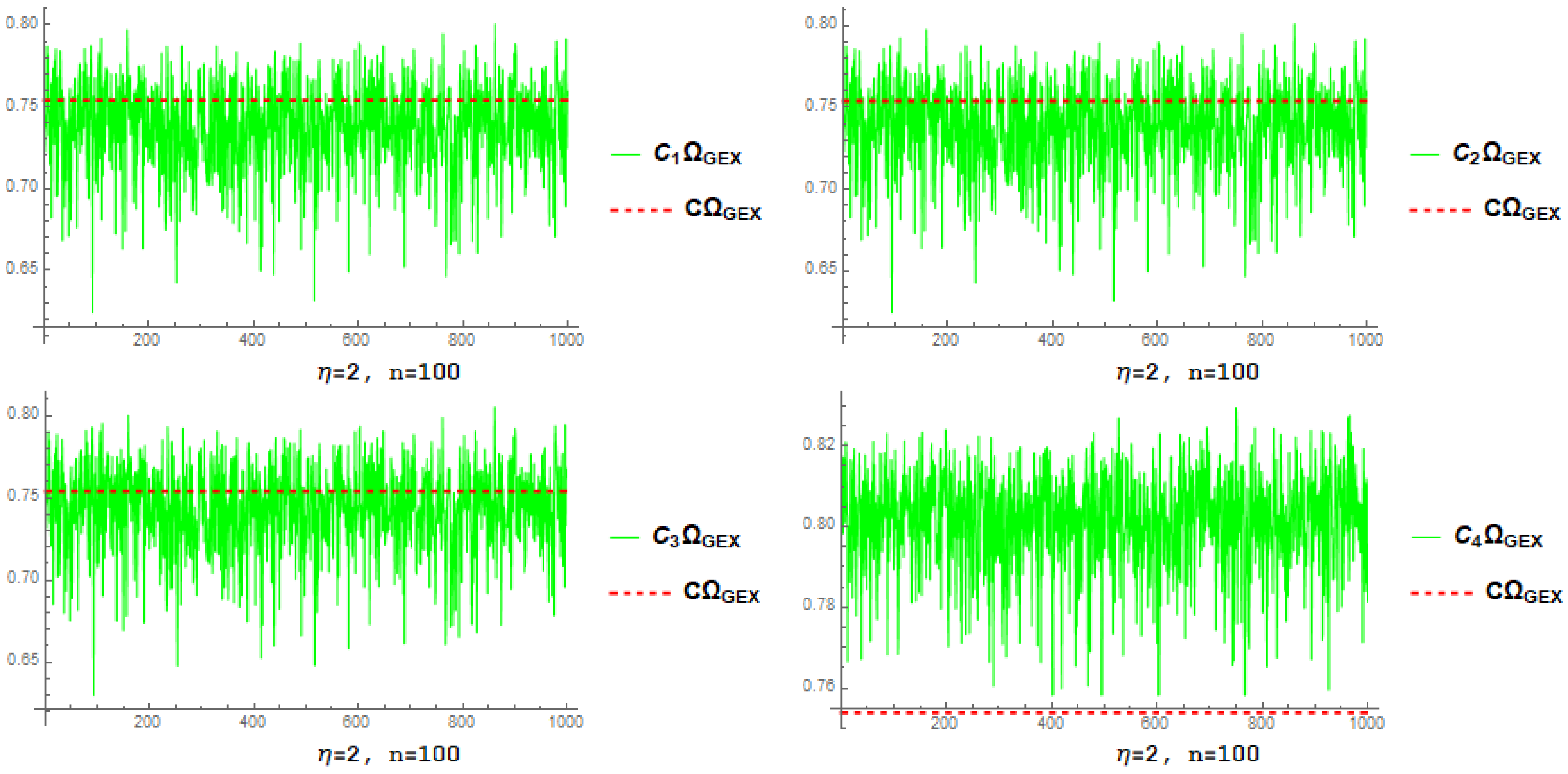
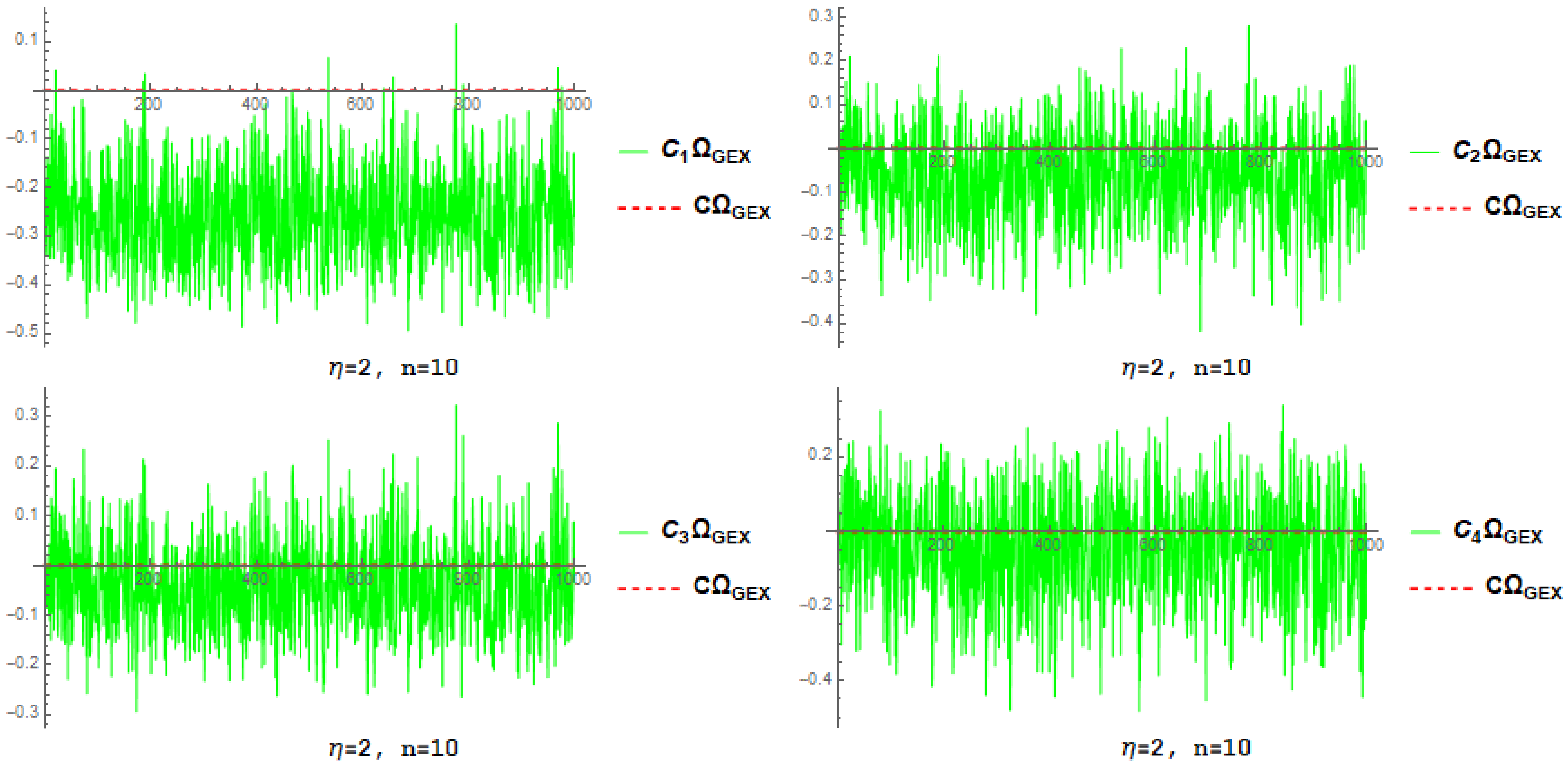
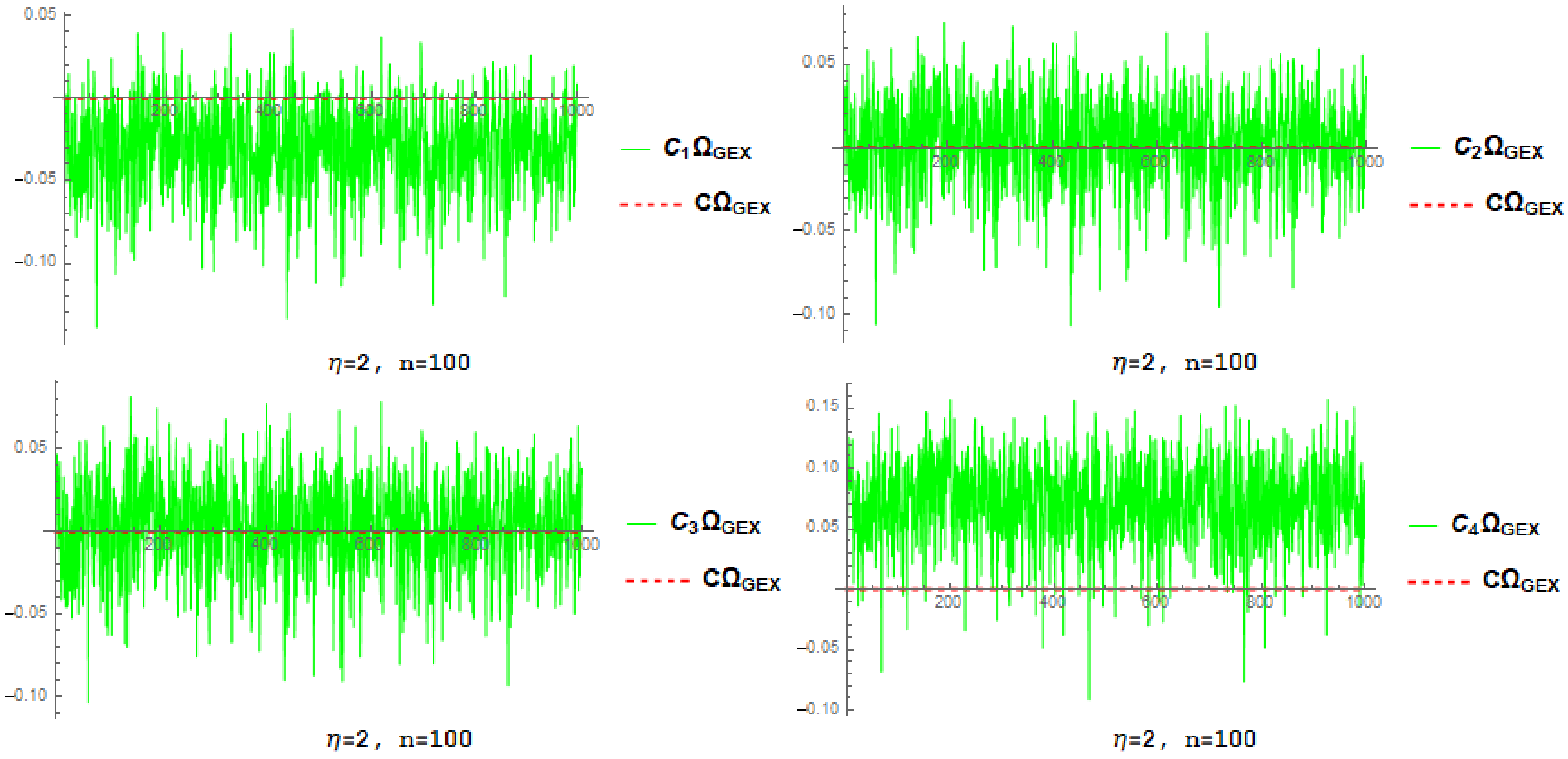
In the present investigation, the performance of the proposed estimators for generalized exponential entropy is investigated using simulations. For each sample size, one thousand samples are created, and the estimators and their root mean squared errors are assessed. The study uses a variety of distributions, such as standard uniform and exponential. The $EXP\left(\gamma \right)$ distribution is implemented in this study using the rate parameter $\gamma =0.5$. Values of the root mean square error and standard deviation for the four generalized exponential entropy estimators for sample sizes $n=10,30,50,100$ for each of the two distributions considered are shown in

Table 1. The standard deviation (in parentheses) and root mean square error for the generalized exponential entropy estimators of the $EXP\left(0.5\right)$ distribution.

	$\mathit{\eta }=2$; $\mathit{C}{\Omega }_{\mathit{GEX}}\left(\mathit{Y}\right)=0.753892$
n	$C_1{\Omega }_{GEX}\left(G_n\right)$	$C_2{\Omega }_{GEX}\left(G_n\right)$	$C_3{\Omega }_{GEX}\left(G_n\right)$	$C_4{\Omega }_{GEX}\left(G_n\right)$
10	0.166619	0.139548	0.131408	0.0676092
	(0.128746)	(0.118047)	(0.113455)	(0.0647867)
30	0.0721833	0.0693193	0.0614541	0.0509792
	(0.0595626)	(0.0589205)	(0.0556205)	(0.0261327)
50	0.0503906	0.0492573	0.0444755	0.0503707
	(0.0430887)	(0.0428833)	(0.0412355)	(0.0180801)
100	0.0322678	0.0319324	0.0290094	0.048996
	(0.0279918)	(0.0279467)	(0.0271723)	(0.0128205)
	$\eta =3$; $C{\Omega }_{GEX}\left(Y\right)=0.545428$
10	0.123315	0.0955782	0.090431	0.0288746
	(0.107512)	(0.0811191)	(0.0779946)	(0.0276784)
30	0.0455141	0.0441009	0.0389924	0.0185159
	(0.0374106)	(0.0368886)	(0.0341483)	(0.00760492)
50	0.0302498	0.029718	0.0268443	0.0184828
	(0.0253976)	(0.0251962)	(0.0238917)	(0.004876)
100	0.0180671	0.0179056	0.0163372	0.0181694
	(0.0151679)	(0.0151121)	(0.0145665)	(0.00331677)

and

Table 2. The standard deviation (in parentheses) and root mean square error for the generalized exponential entropy estimators of the $U(0,1)$ distribution.

	$\mathit{\eta }=2$; $\mathit{C}{\Omega }_{\mathit{GEX}}\left(\mathit{Y}\right)=0$
n	$C_1{\Omega }_{GEX}\left(G_n\right)$	$C_2{\Omega }_{GEX}\left(G_n\right)$	$C_3{\Omega }_{GEX}\left(G_n\right)$	$C_4{\Omega }_{GEX}\left(G_n\right)$
10	0.274905	0.126526	0.104323	0.158303
	(0.101703)	(0.11006)	(0.0963832)	(0.151793)
30	0.0956154	0.0553293	0.0598109	0.0902685
	(0.0578994)	(0.0553003)	(0.0598273)	(0.0799785)
50	0.0659172	0.0426288	0.0450114	0.0827768
	(0.0429443)	(0.0423997)	(0.0448721)	(0.0565385)
100	0.0416265	0.0287682	0.030048	0.0804643
	(0.0281866)	(0.0286104)	(0.0298927)	(0.0371721)
	$\eta =3$; $C{\Omega }_{GEX}\left(Y\right)=0$
10	0.170787	0.0728147	0.0725207	0.111723
	(0.0648594)	(0.0687118)	(0.0652757)	(0.108251)
30	0.0647521	0.0392415	0.0481893	0.0745462
	(0.04087)	(0.0385893)	(0.0463916)	(0.0668339)
50	0.0535745	0.0328033	0.0383248	0.069018
	(0.0322633)	(0.0316971)	(0.0361227)	(0.0498909)
100	0.0431192	0.0264828	0.0280886	0.0675841
	(0.0225317)	(0.023074)	(0.0249522)	(0.0355629)

and Figure 11, Figure 12, Figure 13 and Figure 14. Therefore, we can obtain the following conclusions:

• By increasing n and fixed $\eta$, the root mean square error and associated standard deviation decrease for each estimator.
• By increasing $\eta$ and fixed n, the root mean square error and associated standard deviation decrease for each estimator.
• The values of each estimator are close to the true value, see Figure 11, Figure 12, Figure 13 and Figure 14.

4.2. Real Data Study

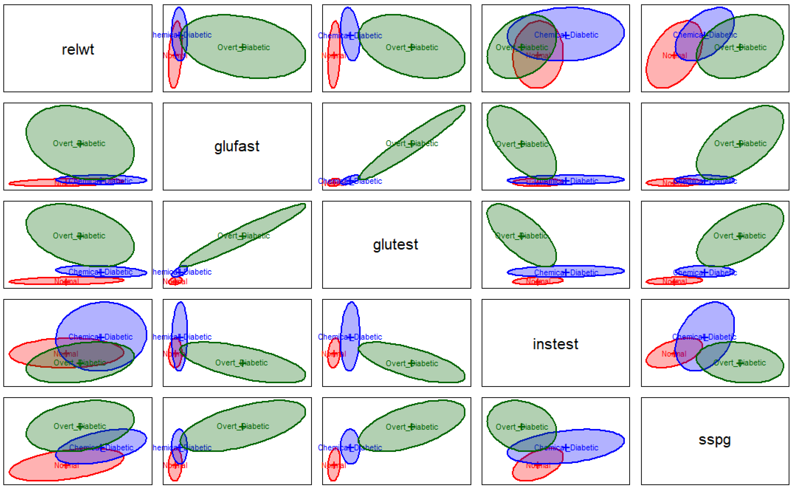
Reaven and Miller [33] investigated the correlation between insulin and blood chemistry indicators of glucose tolerance in 145 individuals who were not fat. After visualizing the data in three dimensions using the Stanford accelerator linear center’s PRIM9 technology, they found an odd pattern that resembled a big blob with two wings pointing in separate directions. The 145 observations were categorized as normal group, overt diabetic group, and sub-clinical (chemical) diabetic group. Five variables were examined for each of the subjects: steady state plasma glucose (sspg), plasma insulin during the test (instest), test plasma glucose level (glutest), fasting plasma glucose level (glufast), and relative weight (relwt). In Figure 15, the covariance ellipses are visualized for exploring these multivariate data and identifying patterns or group differences. Each ellipse illustrates the links between variable pairs by representing the distribution and orientation of data for a particular group. Stronger linear relationships (high covariance) are shown by elongated ellipses. Low covariance, or little to no linear connection, is indicated by circular ellipses. The diversity within the group is represented by the ellipse size: larger ellipses signify greater variability. Therefore, we can see that variances are greatest in the overtly diabetic group and least in the normal group.

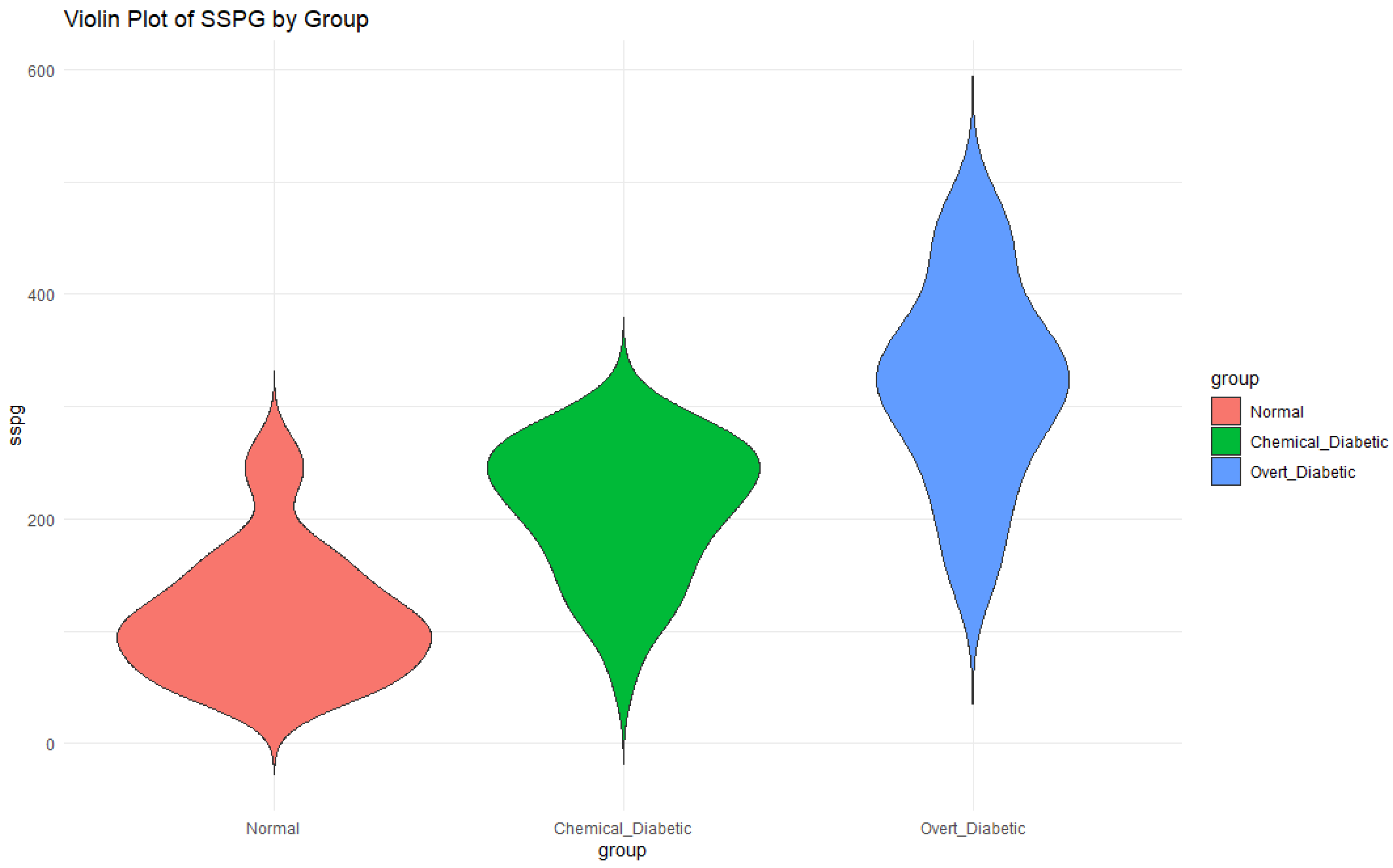
In this study, we choose the sspg set of data to discuss the four generalized exponential entropy estimators. The violin plot, a statistical data visualization that combines the characteristics of a box plot and a kernel density plot, is depicted in Figure 16. It is very helpful for comparing different distributions and displaying the data’s distribution. The box plot, which displays the median, quartiles, and potential outliers, is embedded within the violin, and the width of the violin shows the density (or frequency) of the data at various levels. Furthermore, for greater aesthetics, density is frequently mirrored along the center axis; alternatively it can be shown one-sided.

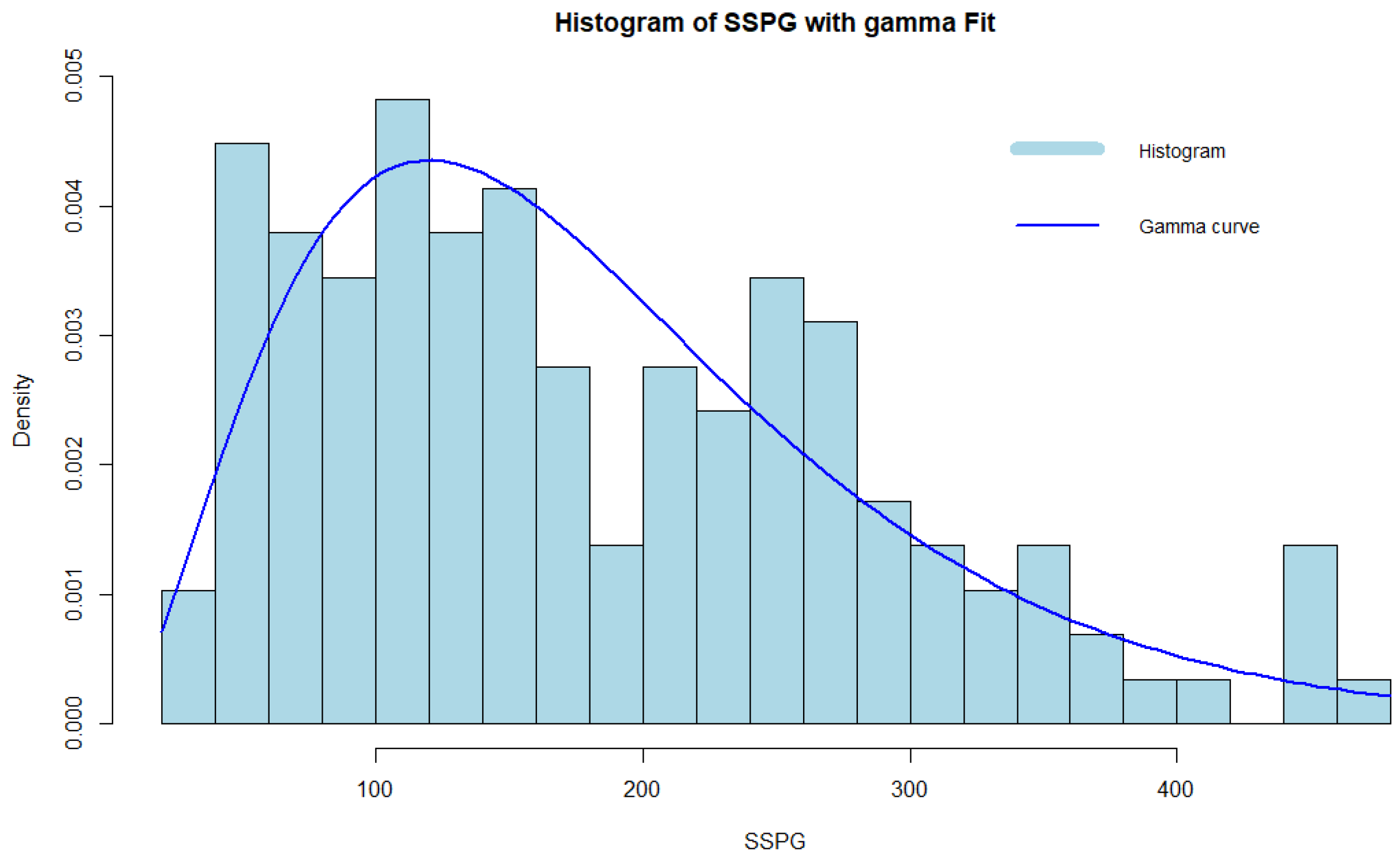
With a shape parameter of 2.880043 and a scale value of 63.95974, we fitted these data to a gamma distribution, whose PDF is given by

$$f(y;a,b)={\displaystyle \frac{y^{a-1}{e}^{-y/b}}{b^a\Gamma \left(a\right)}}\mathrm{for}a,b,y>0.$$

The Kolmogorov–Smirnov (Ko-Sm) test is used to verify that the gamma distribution is a suitable match for the sspg dataset. The gap between the empirical and fitted distribution functions has a Ko-Sm statistic of 0.068327 and a corresponding p-value of 0.5076. Consequently, it makes sense to fit the data using the gamma distribution, as shown in Figure 17.

Table 3. The generalized exponential entropy estimators and their absolute biases (in parentheses) of the sspg set of data.

		Estimators
$\mathit{\eta }$	$\mathit{C}{\Omega }_{\mathit{GEX}}\left(\mathit{Y}\right)$	${\mathit{C}}_{\mathbf{1}}{\Omega }_{\mathit{GEX}}\left({\mathit{G}}_{\mathit{n}}\right)$	${\mathit{C}}_{\mathbf{2}}{\Omega }_{\mathit{GEX}}\left({\mathit{G}}_{\mathit{n}}\right)$	${\mathit{C}}_{\mathbf{3}}{\Omega }_{\mathit{GEX}}\left({\mathit{G}}_{\mathit{n}}\right)$	${\mathit{C}}_{\mathbf{4}}{\Omega }_{\mathit{GEX}}\left({\mathit{G}}_{\mathit{n}}\right)$
0.7	2.39022	2.39562	2.39602	2.39631	2.39382
		(0.00549344)	(0.00584758)	(0.00611249)	(0.00359942)
0.9	1.89316	1.8946	1.89468	1.89479	1.89445
		(0.00144317)	(0.00152767)	(0.00163561)	(0.00129579)
1	1.71011	1.71085	1.7109	1.71096	1.71087
		(0.000742883)	(0.000786553)	(0.000855934)	(0.000765248)
1.5	1.1452	1.14523	1.14523	1.14524	1.14525
		(0.0000300966)	(0.000032158)	(0.0000380813)	(0.0000512178)
2	0.859141	0.859128	0.859128	0.859128	0.85913
		(0.0000129779)	(0.0000129042)	(0.0000125223)	(0.000011189)

shows the four generalized exponential entropy estimators of the sspg set of data for different values of $\eta$ with their absolute biases. Additionally, by raising $\eta$, the absolute biases decrease, and we can see the near values between the estimators and the true value.

5. Statistics for Evaluating the Uniformity Hypothesis Test

In this part, we examine how applying the successful estimate of generalized exponential entropy to the Monte Carlo experiment might enhance the extensions of the entropy-based test of uniformity. In many real-world applications, analyzing uniformity is important since determining goodness-of-fit frequently entails examining uniformity. Let us say we have a random sample of size n, such as $Z_1,Z_2,\dots ,Z_n$, taken from a population that is represented by an unknown CDF, G. Thus, the above goodness-of-fit issue, where G is the CDF of $Z_t$ for $t=1,\dots ,n$, is equivalent to analyzing the null hypothesis $N_0:G\left(z\right)=z$ for all $z\in (0,1)$, as opposed to $N_1:G\left(z\right)\ne z$ for some $z\in (0,1)$. A detailed review of testing uniformity research is given by Marhuenda et al. [34], who also provide a lengthy list of references (also see Sakr and Mohamed [17] and Qiu and Jia [14]).

Theorem 3.

Assume that the random variable Z follows a standard uniform distribution $U(0,1)$. Then, from (11), $C{\Omega }_{GEX}\left(Z\right)=0$ if Z follows $U(0,1)$ distribution.

In line with the generalized exponential entropy estimates $C_j{\Omega }_{GEX}\left(G_n\right)$, $j=1,2,3,4$, given in (19)–(21) and (24), respectively, and under the null hypothesis $G\left(z\right)=z$ for all $y\in (0,1)$, we get (i.e., $\underset{\mathrm{Pr}.}{\to }$ refers to converges in probability)

$$\begin{array}{c}\hfill C_j{\Omega }_{GEX}\left(G_n\right)\underset{\mathrm{Pr}.}{\to }0,whenn⟶\infty .\end{array}$$

Taking into account a different distribution where the PDF h and CDF H are specified on the interval $(0,1)$, we get

$$\begin{array}{c}\hfill C_j{\Omega }_{GEX}\left(H_n\right)\underset{\mathrm{Pr}.}{\to }C{\Omega }_{GEX}\left(Y\right)\ne 0,whenn⟶\infty .\end{array}$$

To evaluate uniformity, we suggest the tests of statistic $C_j{\Omega }_{GEX}\left(G_n\right)$, $j=1,2,3,4$, in accordance with the technique developed by Zamanzade and Arghami [35]. We reject the uniformity hypothesis when $C_j{\Omega }_{GEX}\left(G_n\right)$ values depart from zero, indicating non-uniformity.

Critical Points of Percentage and Power Analysis Comparisons

Unfavorably we are unable to ascertain the precise distribution of the statistics $C_j{\Omega }_{GEX}\left(G_n\right)$ based on the null hypothesis due to the intricacy of the tests. In order to determine its critical values, we employ Monte Carlo simulation. We use the Monte Carlo method to obtain the percentage points under the generalized exponential entropy estimations. The area necessary to establish the uniformity test is described by the interval

$$[lowerlevel,upperlevel]:=[C_j{\Omega }_{GEX}^{{\displaystyle \frac{\alpha }{2}}},C_j{\Omega }_{GEX}^{1-{\displaystyle \frac{\alpha }{2}}}],j=1,2,3,4,$$

where $\alpha$ denotes the selected significance level, and $C_j{\Omega }_{GEX}^{\alpha }$ represents the $\alpha$-quantile function, based on the null hypothesis, of the nearly or asymptotic CDF test statistic.

At the significance level of $0.05$, the crucial points of the percentage of the tests of the statistic $C_j{\Omega }_{GEX}\left(G_n\right)$, $j=1,2,3,4$, are shown in

Table 4. At the significance level of $0.05$, the limits of the percentage points of the generalized exponential entropy estimators with $\eta =2,3$.

n; $\mathit{\eta }=2$	${\mathit{C}}_1{\Omega }_{\mathit{GEX}}\left({\mathit{G}}_{\mathit{n}}\right)$	${\mathit{C}}_2{\Omega }_{\mathit{GEX}}\left({\mathit{G}}_{\mathit{n}}\right)$	${\mathit{C}}_3{\Omega }_{\mathit{GEX}}\left({\mathit{G}}_{\mathit{n}}\right)$	${\mathit{C}}_4{\Omega }_{\mathit{GEX}}\left({\mathit{G}}_{\mathit{n}}\right)$
10	(−0.422986, −0.0150384)	(−0.284684, 0.177716)	(−0.177159, 0.189558)	(−0.22324, 0.210542)
20	(−0.248859, 0.0333156)	(−0.141655, 0.128236)	(−0.123249, 0.146506)	(−0.154934, 0.172644)
30	(−0.183537, 0.0377545)	(−0.104446, 0.105192)	(−0.105972, 0.119938)	(−0.0959191, 0.159991)
50	(−0.132261, 0.0346427)	(−0.0734596, 0.0868403)	(−0.0753921, 0.0944493)	(−0.0301963, 0.146967)
70	(−0.105717, 0.0274583)	(−0.0676648, 0.0664032)	(−0.0706697, 0.0746701)	(−0.0193603, 0.136071)
100	(−0.086409, 0.0198325)	(−0.0565094, 0.0536249)	(−0.056399, 0.0581039)	(−0.00358996, 0.126684)
n; $\eta =3$	$C_1{\Omega }_{GEX}\left(G_n\right)$	$C_2{\Omega }_{GEX}\left(G_n\right)$	$C_3{\Omega }_{GEX}\left(G_n\right)$	$C_4{\Omega }_{GEX}\left(G_n\right)$
10	(0.147299, 0.3406)	(0.0325989, 0.33247)	(−0.121961, 0.173553)	(−0.187423, 0.195208)
20	(−0.0827349, 0.0755373)	(−0.0731537, 0.118101)	(−0.115785, 0.120527)	(−0.136084, 0.161355)
30	(−0.105273, 0.0551253)	(−0.077303, 0.0866788)	(−0.103773, 0.0997682)	(−0.0913948, 0.149395)
50	(−0.0974539, 0.032796)	(−0.0648665, 0.0697503)	(−0.0795326, 0.0741954)	(−0.0335902, 0.136741)
70	(−0.0884423, 0.0204563)	(−0.0634696, 0.0511093)	(−0.0700712, 0.055357)	(−0.021843, 0.127675)
100	(−0.0837358, 0.0115276)	(−0.0597903, 0.0369845)	(−0.0654341, 0.0408905)	(−0.00320919, 0.119708)

, for varying sample numbers $n=10,20,30,50,70,100$, derived from 1000-iteration Monte Carlo simulations. Then, we can observe that

• By increasing the sample size n, the difference in percentage points decreases.
• For fixed n and increasing $\eta$, the difference in percentage points decreases.
• Most of the four estimators yield percentage point intervals that include the true value (i.e., zero) of the generalized exponential entropy measure of the $U(0,1)$ distribution across different values of n and $\eta$, with few exceptions at small n.

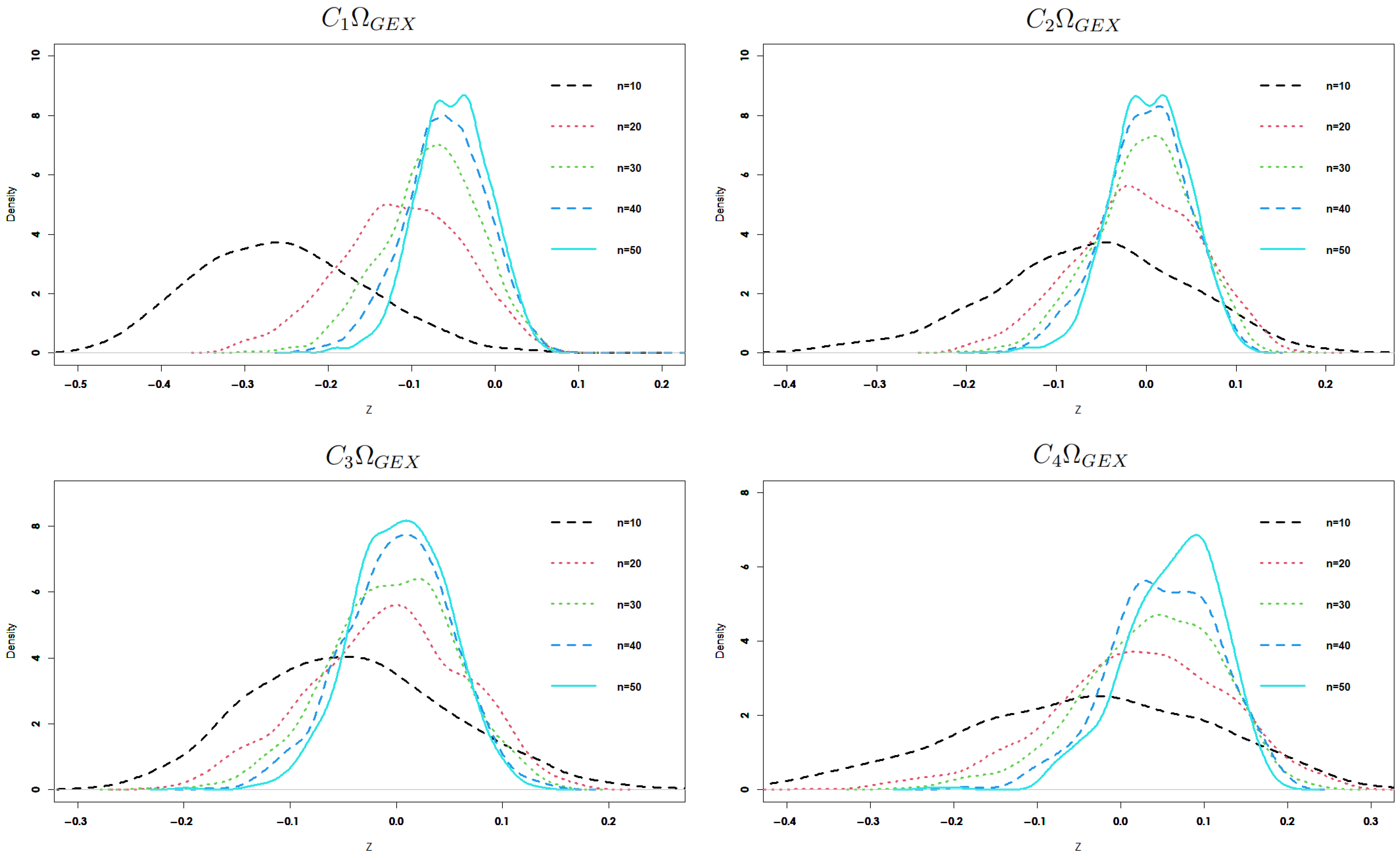
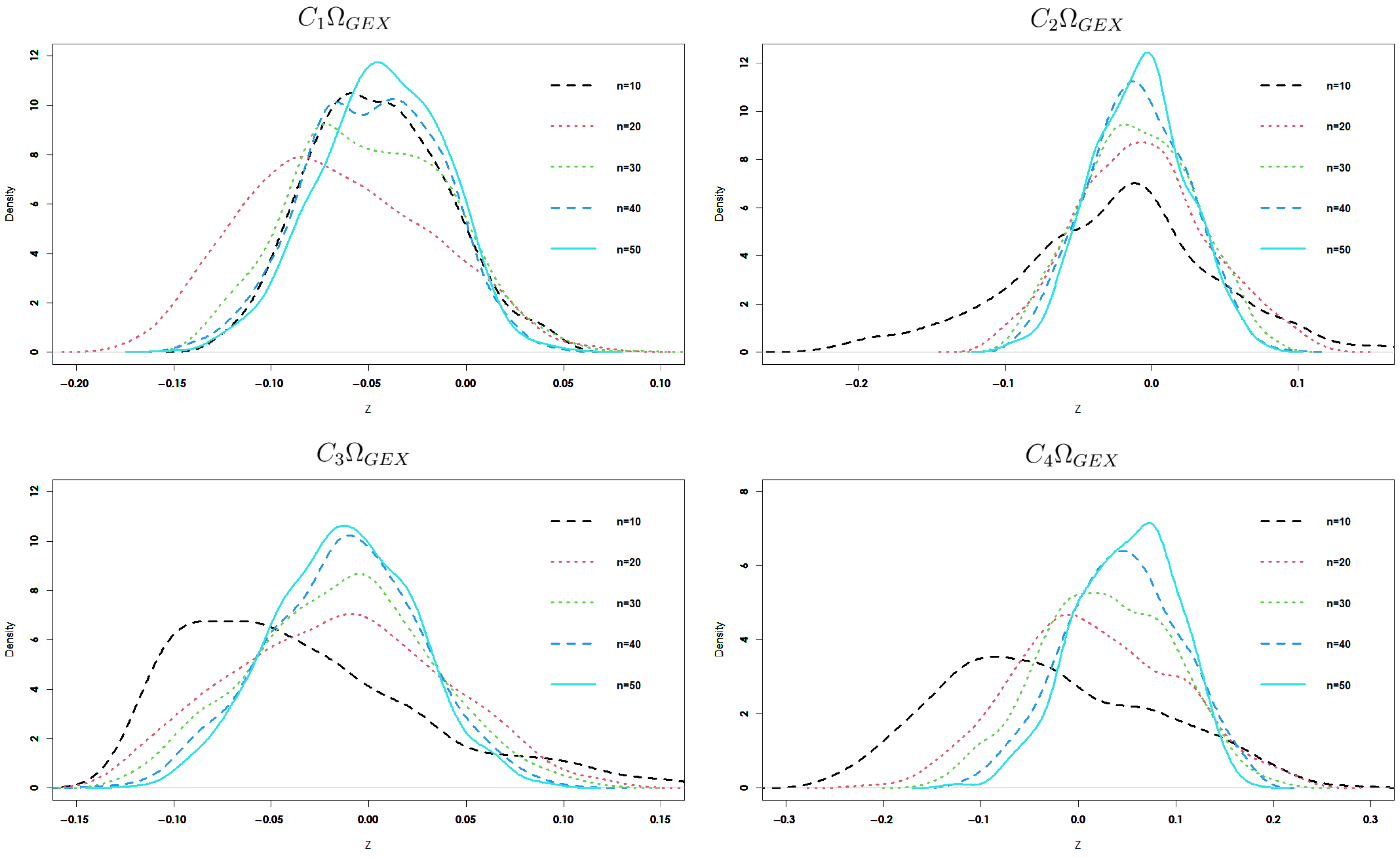
The densities of the various generalized exponential entropy estimators for $n=10,20,30,40,50$ and $\eta =2,4$ are displayed in Figure 18 and Figure 19. It is seen that the test statistics become closer to the exact values (zero) as n increases, indicating that bias and variance both reduce with increasing n.

We evaluate the efficacy of our suggested tests using Monte Carlo simulations by contrasting their capabilities under seven possible situations and with those of other tests. Several researchers have studied a variety of options in uniformity testing, such as Zamanzade [35] and Qiu and Jia [14]. Based on the forms of their densities, they have divided them into three groups as follows:

$$\begin{array}{cc}\hfill & {\mho }_1^{\omega }:G\left(z\right)=1-{(1-z)}^{\omega },0\le z\le 1,\omega =1.5,2,\hfill \\ & {\mho }_2^{\omega }:G\left(z\right)=\left\{\begin{array}{c}{2}^{\omega -1}{z}^{\omega },0\le z\le 0.5,\hfill \\ 1-2^{\omega -1}{(1-z)}^{\omega },0.5\le z\le 1,\omega =1.5,2,3,\hfill \end{array}\right.\hfill \\ & {\mho }_3^{\omega }:G\left(z\right)=\left\{\begin{array}{c}0.5-2^{\omega -1}{(0.5-z)}^{\omega },0\le z\le 0.5,\hfill \\ 0.5+2^{\omega -1}{(z-0.5)}^{\omega },0.5\le z\le 1,\omega =1.5,2.\hfill \end{array}\right.\hfill \end{array}$$

We evaluate the effectiveness of our suggested test statistic in comparison with several established statistics under identical alternatives as follows:

• The statistic of the Cramer–von Mises test (Cramer [36]):

  $$C\&M=\sum _{t=1}^n\left(Z_{(t;n)}-{\displaystyle \frac{2t-1}{2n}}\right)+{\displaystyle \frac{1}{12n}}.$$

  (34)
• The statistic of the Kolmogrov–Smirnov test (Kolmogorov [37]):

  $$K\&S=max\left(\underset{1\le t\le n}{max}\left({\displaystyle \frac{t}{n}}-Z_{(t;n)}\right),\underset{1\le t\le n}{max}\left(Z_{(t;n)}-{\displaystyle \frac{t-1}{n}}\right)\right).$$

  (35)
• The statistic of the Anderson–Darling test (Anderson and Darling [38]):

  $$A\&D={\displaystyle \frac{-2}{n}}\sum _{t=1}^n\left((t-0.5)log\left(Z_{(t;n)}\right)+(n-t+0.5)log(1-Z_{(t;n)})\right)-n.$$

  (36)
• The statistic of the extropy test (Qiu and Jia [14]):

  $${\chi }_{EX}={\displaystyle \frac{-1}{2n}}\sum _{t=1}^n{\displaystyle \frac{{\Xi }_{t}r/n}{\left(Z_{(t+r;n)}-Z_{(t-r;n)}\right)}},$$

  (37)

  where the positive integer window size $r<{\displaystyle \frac{n}{2}}$ and $Z_t=Z_1$ if $t<1$ and $Z_t=Z_n$ if $t>n$, and ${\Xi }_t$ is defined in (10).

Remark 1.

In our simulation study, we focus on evaluating the power of the proposed uniformity test under small sample sizes $(n=10,20,30)$. This choice reflects practical scenarios where uniformity testing is applied to limited data. Our goal is to assess the finite-sample performance and sensitivity of the test, rather than to explore asymptotic properties. Power analysis in this context provides meaningful insights into the test’s effectiveness when applied to real-world problems with restricted sample sizes. Moreover, small samples are justified in power studies for many reasons:

1. 

Power analysis under small n is crucial: in practice, uniformity tests are often used in settings with limited data (e.g., simulation diagnostics, goodness-of-fit checks in applied sciences). Knowing how the test performs with small samples is highly valuable.

2. 

Since we are not using these sample sizes to justify theoretical properties like asymptotic normality, but instead focusing on finite-sample power, small n is appropriate.

3. 

It shows practical sensitivity: if your test has good power at $n=10,20,30$, this highlights its sensitivity and usefulness in realistic, data-limited conditions.

Unfavorably, the strengths of certain suggested tests change depending on the alternative distributions and window size. Finding the ideal value of $\lambda$ that optimizes the test’s power for every possibility is therefore not possible. To ensure the efficacy of the proposed test, which attains sufficient (although not ideal) power over all potential distributions as described in (33), we use the associated heuristic formula to determine $\lambda$. In order to avoid the central limit theorem and preserve normalcy, we also choose $n=10,20,30$ as the sample size n and do not go over this. The power analysis comparison estimates at a significance level of 0.05 with $\eta =2,3$ are provided in

Table 5. Power value estimations of the various statistics are compared at a significance level of 0.05, using $\eta =2,3$.

n	Alt.	Statistics; $\mathit{\eta }=2$				$\mathit{K}\&\mathit{S}$	$\mathit{A}\&\mathit{D}$	$\mathit{C}\&\mathit{M}$	${\mathit{\chi }}_{\mathit{EX}}$
		${\mathit{C}}_{\mathbf{1}}{\Omega }_{\mathit{GEX}}\left({\mathit{G}}_{\mathit{n}}\right)$	${\mathit{C}}_{\mathbf{2}}{\Omega }_{\mathit{GEX}}\left({\mathit{G}}_{\mathit{n}}\right)$	${\mathit{C}}_{\mathbf{3}}{\Omega }_{\mathit{GEX}}\left({\mathit{G}}_{\mathit{n}}\right)$	${\mathit{C}}_{\mathbf{4}}{\Omega }_{\mathit{GEX}}\left({\mathit{G}}_{\mathit{n}}\right)$
10	${\mho }_1^{1.5}$	0.114	0.075	0.23	0.421	0.152	0.166	0.168	0.129
	${\mho }_1^2$	0.241	0.148	0.465	0.698	0.376	0.409	0.438	0.32
	${\mho }_2^{1.5}$	0.247	0.176	0.314	0.416	0.037	0.015	0.026	0.21
	${\mho }_2^2$	0.585	0.435	0.618	0.688	0.044	0.009	0.022	0.455
	${\mho }_2^3$	0.946	0.867	0.885	0.94	0.087	0.018	0.051	0.801
	${\mho }_3^{1.5}$	0.101	0.087	0.159	0.117	0.113	0.121	0.098	0.082
	${\mho }_3^2$	0.3	0.209	0.552	0.147	0.199	0.227	0.155	0.131
20	${\mho }_1^{1.5}$	0.178	0.193	0.305	0.546	0.279	0.309	0.324	0.258
	${\mho }_1^2$	0.47	0.495	0.644	0.868	0.699	0.756	0.771	0.665
	${\mho }_2^{1.5}$	0.443	0.411	0.51	0.607	0.059	0.032	0.042	0.399
	${\mho }_2^2$	0.878	0.862	0.881	0.912	0.125	0.092	0.100	0.808
	${\mho }_2^3$	1	1	0.994	1	0.410	0.537	0.513	0.991
	${\mho }_3^{1.5}$	0.147	0.09	0.128	0.062	0.150	0.156	0.119	0.155
	${\mho }_3^2$	0.412	0.188	0.522	0.085	0.315	0.371	0.250	0.363
30	${\mho }_1^{1.5}$	0.281	0.319	0.336	0.723	0.520	0.592	0.594	0.529
	${\mho }_1^2$	0.693	0.739	0.742	0.974	0.955	0.978	0.978	0.919
	${\mho }_2^{1.5}$	0.608	0.606	0.586	0.794	0.113	0.108	0.093	0.581
	${\mho }_2^2$	0.963	0.971	0.943	0.992	0.376	0.560	0.445	0.924
	${\mho }_2^3$	1	1	0.999	1	0.928	0.996	0.986	1
	${\mho }_3^{1.5}$	0.131	0.095	0.153	0.049	0.230	0.241	0.175	0.217
	${\mho }_3^2$	0.248	0.123	0.343	0.07	0.561	0.695	0.557	0.782
n	Alt.	Statistics; $\mathit{\eta }=3$				$\mathit{K}\&\mathit{S}$	$\mathit{A}\&\mathit{D}$	$\mathit{C}\&\mathit{M}$	${\mathit{\chi }}_{\mathit{EX}}$
		${\mathit{C}}_{\mathbf{1}}{\Omega }_{\mathit{GEX}}\left({\mathit{G}}_{\mathit{n}}\right)$	${\mathit{C}}_{\mathbf{2}}{\Omega }_{\mathit{GEX}}\left({\mathit{G}}_{\mathit{n}}\right)$	${\mathit{C}}_{\mathbf{3}}{\Omega }_{\mathit{GEX}}\left({\mathit{G}}_{\mathit{n}}\right)$	${\mathit{C}}_{\mathbf{4}}{\Omega }_{\mathit{GEX}}\left({\mathit{G}}_{\mathit{n}}\right)$
10	${\mho }_1^{1.5}$	0.129	0.107	0.259	0.447	0.152	0.166	0.168	0.129
	${\mho }_1^2$	0.263	0.188	0.576	0.718	0.376	0.409	0.438	0.32
	${\mho }_2^{1.5}$	0.297	0.219	0.346	0.43	0.037	0.015	0.026	0.21
	${\mho }_2^2$	0.589	0.571	0.651	0.7	0.044	0.009	0.022	0.455
	${\mho }_2^3$	0.949	0.87	0.889	0.95	0.087	0.018	0.051	0.801
	${\mho }_3^{1.5}$	0.115	0.112	0.176	0.12	0.113	0.121	0.098	0.082
	${\mho }_3^2$	0.257	0.122	0.567	0.149	0.199	0.227	0.155	0.131
20	${\mho }_1^{1.5}$	0.136	0.242	0.329	0.551	0.279	0.309	0.324	0.258
	${\mho }_1^2$	0.499	0.531	0.684	0.876	0.699	0.756	0.771	0.665
	${\mho }_2^{1.5}$	0.447	0.599	0.616	0.612	0.059	0.032	0.042	0.399
	${\mho }_2^2$	0.813	0.739	0.873	0.917	0.125	0.092	0.100	0.808
	${\mho }_2^3$	1	1	1	1	0.410	0.537	0.513	0.991
	${\mho }_3^{1.5}$	0.156	0.11	0.163	0.062	0.150	0.156	0.119	0.155
	${\mho }_3^2$	0.417	0.282	0.653	0.091	0.315	0.371	0.250	0.363
30	${\mho }_1^{1.5}$	0.302	0.343	0.351	0.748	0.520	0.592	0.594	0.529
	${\mho }_1^2$	0.698	0.788	0.788	0.977	0.955	0.978	0.978	0.919
	${\mho }_2^{1.5}$	0.702	0.726	0.608	0.798	0.113	0.108	0.093	0.581
	${\mho }_2^2$	0.968	0.985	0.966	0.998	0.376	0.560	0.445	0.924
	${\mho }_2^3$	1	1	1	1	0.928	0.996	0.986	1
	${\mho }_3^{1.5}$	0.167	0.17	0.176	0.052	0.230	0.241	0.175	0.217
	${\mho }_3^2$	0.255	0.266	0.388	0.059	0.561	0.695	0.557	0.782

. Then, it is evident that

• In contrast to the previous tests, the four generalized exponential entropy estimators behave well under different ${\mho }_2^{\omega }$. Alternatives ${\mho }_1^{\omega }$, ${\mho }_2^{\omega }$, and ${\mho }_3^{\omega }$ were interpreted by Stephens [39] as suggesting a shift in the mean, a change towards a lower variance, and a shift towards a greater variance, respectively. As a result, when there is a movement towards a lower variance, our tests perform better than alternatives.
• By increasing the value of $\eta$, our four proposed estimators increase in power.
• Across a range of n values, the fourth statistic, which is based on the kernel function, performs better than all other tests under alternatives ${\mho }_1^{\omega }$ and ${\mho }_2^{\omega }$.

6. Conclusions

In this article, we introduced the continuous case of generalized exponential entropy with some applications to well-known distributions and found that this model tends to classical Shannon entropy when $\eta \to 0$. We discussed the complementary dual of generalized exponential entropy and its approximation, and noted that this approximation yields the same approximation of the complementary dual of entropy, which is known as extropy. We provided a number of non-parametric estimation techniques and assessed their asymptotic normalcy using Monte Carlo simulation. In the fourth technique of estimation, we applied kernel estimation under ${\rho }_{corr}$-mixing dependent data and discussed its consistency and biases. We implemented simulation and real data to evaluate the proposed estimators. Finally, we analyzed critical points of percentage and power comparisons using the four generalized exponential entropy estimators to test uniformity. We observed that the value of the parameter $\eta$ significantly affects the results.

Despite these contributions, the study has some limitations. First, while the simulation results are promising, the scope of real data analysis is limited, and additional case studies could further validate the estimator’s robustness. Second, the analysis focuses primarily on univariate settings, and extending the model to multivariate contexts remains an open challenge. Third, the kernel-based estimator under ${\rho }_{\mathrm{corr}}$-mixing assumes specific dependence structures that may not capture all forms of real-world dependency, potentially limiting generalizability. Lastly, some theoretical properties such as the optimal bandwidth selection and finite-sample behavior were not exhaustively explored.

For future research, we plan to conduct more extensive real data analyses to further highlight the potential of the proposed estimator in applied settings. In particular, we aim to develop and evaluate statistical tests based on this entropy measure to enhance its applicability in inference problems. Additionally, a more detailed investigation of the covariance structure in real datasets will be considered to better understand its influence on the performance and interpretation of the proposed model. Furthermore, a more explicit report on the empirical Type I error (i.e., rejection rate under the null hypothesis) would enhance the completeness of the study. Moreover, we can apply this study for the dynamic version of the uncertainty measures; see, for example, Mohamed and Sakr [40].

References

1. Shannon, C. A mathematical theory of communication. Bell Syst. Tech. J. 1948, 27, 379–423. [Google Scholar] [CrossRef]
2. Renyi, A. On measures of entropy and information. In Proceedings of the Fourth Berkeley Symposium on Mathematical Statistics and Probability, Berkeley, CA, USA, 20–30 July 1960; UC Press, Berkeley: Berkeley, CA, USA, 1961; pp. 547–561. [Google Scholar]
3. Kapur, J.N. Generalized entropy of order α and type β. Math. Semin. 1967, 4, 78–82. [Google Scholar]
4. Havrda, J.; Charvat, F. Qualification method of classification process: The concept of structural α-entropy. Kybernetika 1967, 3, 30–35. [Google Scholar]
5. Tsallis, C. Possible generalization of Boltzmann-Gibbs statistics. J. Stat. Phys. 1988, 52, 479–487. [Google Scholar] [CrossRef]
6. Pal, N.R.; Pal, S.K. Object background segmentation using new definitions of entropy. IEEE Proc. 1989, 136, 284–295. [Google Scholar] [CrossRef]
7. Pal, N.R.; Pal, S.K. Entropy: A new definition and its applications. IEEE Trans. Syst. Man Cybern. 1991, 21, 1260–1270. [Google Scholar] [CrossRef]
8. Campbell, L.L. Exponential entropy as a measure of extent of distribution. Z. Wahrscheinlichkeitstheorie Verwandte Geb. 1966, 5, 217–225. [Google Scholar] [CrossRef]
9. Panjehkeh, S.M.; Borzadaran, G.R.M.; Amini, M. Results related to exponential entropy. Int. Inf. Coding Theory 2017, 4, 258–275. [Google Scholar] [CrossRef]
10. Kvalseth, T.O. On exponential entropies. In Proceedings of the IEEE International Conference on Systems, Man And Cybernatics 2000, Nashville, TN, USA, 8–11 October 2000; Volume 4, pp. 2822–2826. [Google Scholar]
11. Lad, F.; Sanfilippo, G.; Agro, G. Extropy: Complementary dual of entropy. Stat. Sci. 2015, 30, 40–58. [Google Scholar] [CrossRef]
12. Vasicek, O. A Test for Normality based on Sample Entropy. J. R. Stat. Soc. Ser. B 1976, 38, 54–59. [Google Scholar] [CrossRef]
13. Ebrahimi, N.; Pflughoeft, K.; Soofi, E.S. Two Measures of Sample Entropy. Stat. Probab. Lett. 1994, 20, 225–234. [Google Scholar] [CrossRef]
14. Qiu, G.; Jia, K. Extropy Estimators with Applications in Testing Uniformity. J. Nonparametric Stat. 2018, 30, 182–196. [Google Scholar] [CrossRef]
15. Noughabi, H.A.; Jarrahiferiz, J. Extropy of order statistics applied to testing symmetry. Commun. Stat.-Simul. 2020, 55, 3389–3399. [Google Scholar] [CrossRef]
16. Wachowiak, M.P.; Smolikova, R.; Tourassi, G.D.; Elmaghraby, A.S. Estimation of generalized entropies with sample spacing. Pattern Anal. Appl. 2005, 8, 95–101. [Google Scholar] [CrossRef]
17. Sakr, H.H.; Mohamed, M.S. Sharma-Taneja-Mittal Entropy and Its Application of Obesity in Saudi Arabia. Mathematics 2024, 12, 2639. [Google Scholar] [CrossRef]
18. Sakr, H.H.; Mohamed, M.S. On residual cumulative generalized exponential entropy and its application in human health. Electron. Res. Arch. 2025, 33, 1633–1666. [Google Scholar] [CrossRef]
19. Rosenblatt, M. A central limit theorem and a strong mixing condition. Proc. Natl. Acad. Sci. USA 1956, 42, 43–47. [Google Scholar] [CrossRef] [PubMed]
20. Ibragimov, I.A. Some limit theorems for stochastic processes stationary in the strict sense. Dokl. Akad. Nauk. SSSR 1959, 125, 711–714. [Google Scholar]
21. Kolmogorov, A.N.; Rozanov, Y.A. On strong mixing conditions for stationary Gaussian processes. Theory Probab. Appl. 1960, 5, 204–208. [Google Scholar] [CrossRef]
22. Bradley, R.C. Central limit theorems under weak dependence. J. Multivar. Anal. 1981, 11, 1–16. [Google Scholar] [CrossRef]
23. Masry, E. Recursive probability density estimation for weakly dependent stationary processes. IEEE Trans. Inf. Theory 1986, 32, 254–267. [Google Scholar] [CrossRef]
24. Rajesh, G.; Abdul-Sathar, E.I.; Maya, R. Local linear estimation of residual entropy function of conditional distribution, Comput. Stat. Data Anal. 2015, 88, 1–14. [Google Scholar] [CrossRef]
25. Irshad, M.R.; Maya, R.; Buono, F.; Longobardi, M. Kernel Estimation of Cumulative Residual Tsallis Entropy and Its Dynamic Version under ρ-Mixing Dependent Data. Entropy 2022, 24, 9. [Google Scholar] [CrossRef] [PubMed]
26. Ye, J.; Cui, W. Exponential Entropy for Simplified Neutrosophic Sets and Its Application in Decision Making. Entropy 2018, 20, 357. [Google Scholar] [CrossRef]
27. Wang, C.; Shi, G.; Sheng, Y.; Ahmadzade, H. Exponential entropy of uncertain sets and its applications to learning curve and portfolio optimization. J. Ind. Manag. 2025, 21, 1488–1502. [Google Scholar] [CrossRef]
28. Wanke, P. The uniform distribution as a first practical approach to new product inventory management. Int. J. Prod. Econ. 2008, 114, 811–819. [Google Scholar] [CrossRef]
29. Correa, J.C. A new Estimator of entropy. Commun. Stat. Theory Methods 1995, 24, 2439–2449. [Google Scholar] [CrossRef]
30. Wegman, E.J.; Davies, H.I. Remarks on some recursive estimators of a probability density. Ann. Stat. 1979, 7, 316–327. [Google Scholar] [CrossRef]
31. Parzen, E. On estimation of a probability density function and mode. Ann. Math. Stat. 1962, 33, 1065–1076. [Google Scholar] [CrossRef]
32. Grzegorzewski, P.; Wieczorkowski, R. Entropy-based Goodness-of-fit Test for Exponentiality. Commun. Stat. Theory Methods 1999, 28, 1183–1202. [Google Scholar] [CrossRef]
33. Reaven, G.M.; Miller, R.G. An attempt to define the nature of chemical diabetes using a multidimensional analysis. Diabetologia 1979, 16, 17–24. [Google Scholar] [CrossRef]
34. Marhuenda, Y.; Morales, D.; Pardo, M.C. A Comparison of Uniformity Tests. Statistics 2005, 39, 315–327. [Google Scholar] [CrossRef]
35. Zamanzade, E.; Arghami, N.R. Goodness-of-Fit Test based on Correcting Moments of Modified Entropy Estimator. J. Stat. Comput. Simul. 2011, 81, 2077–2093. [Google Scholar] [CrossRef]
36. Cramér, H. On the Composition of Elementary Errors: II. Stat. Appl. Scand. Actuar. J. 1928, 1, 141–180. [Google Scholar] [CrossRef]
37. Kolmogorov, A.N. Sulla Determinazione Empirica di una Legge di Distibuziane. G. Dell’Istitutaitaliano Attuari 1933, 4, 83–91. [Google Scholar]
38. Anderson, W.T.; Darling, A.D. A Test of Goodness-of-Fit. J. Am. Stat. Assoc. 1954, 49, 765–769. [Google Scholar] [CrossRef]
39. Stephens, M.A. EDF statistics for goodness of fit and some comparisons. J. Am. Stat. Assoc. 1974, 69, 730–737. [Google Scholar] [CrossRef]
40. Mohamed, M.S.; Sakr, H.H. Generalizing Uncertainty Through Dynamic Development and Analysis of Residual Cumulative Generalized Fractional Extropy with Applications in Human Health. Fractal Fract. 2025, 9, 388. [Google Scholar] [CrossRef]
Figure 1. Plot of the generalized exponential entropy of exponential distribution with γ = 0.5 , 1 , 1.5 , 2 .
Symmetry 17 01403 g001
Figure 2. Plot of the complete differential complementary dual of generalized exponential entropy and entropy of E X P ( 1 ) distribution.
Symmetry 17 01403 g002
Figure 3. Histogram of Δ 1 with η = 2 (left) and η = 3 (right), and n = 50 .
Symmetry 17 01403 g003
Figure 4. Histogram of Δ 1 with η = 2 (left) and η = 3 (right), and n = 100 .
Symmetry 17 01403 g004
Figure 5. Histogram of Δ 2 with η = 2 (left) and η = 3 (right), and n = 50 .
Symmetry 17 01403 g005
Figure 6. Histogram of Δ 2 with η = 2 (left) and η = 3 (right), and n = 100 .
Symmetry 17 01403 g006
Figure 7. Histogram of Δ 3 with η = 2 (left) and η = 3 (right), and n = 50 .
Symmetry 17 01403 g007
Figure 8. Histogram of Δ 3 with η = 2 (left) and η = 3 (right), and n = 100 .
Symmetry 17 01403 g008
Figure 9. Histogram of Δ 4 with η = 2 (left) and η = 3 (right), and n = 50 .
Symmetry 17 01403 g009
Figure 10. Histogram of Δ 4 with η = 2 (left) and η = 3 (right), and n = 100 .
Symmetry 17 01403 g010
Figure 11. Generalized exponential entropy of E X P ( 0.5 ) with η = 2 and n = 10 .
Symmetry 17 01403 g011
Figure 12. Generalized exponential entropy of E X P ( 0.5 ) with η = 2 and n = 100 .
Symmetry 17 01403 g012
Figure 13. Generalized exponential entropy of U ( 0 , 1 ) with η = 2 and n = 10 .
Symmetry 17 01403 g013
Figure 14. Generalized exponential entropy of U ( 0 , 1 ) with η = 3 and n = 100 .
Symmetry 17 01403 g014
Figure 15. Covariance ellipses of the data.
Symmetry 17 01403 g015
Figure 16. Violin plot of SSPG by group.
Symmetry 17 01403 g016
Figure 17. Histogram of SSPG with gamma distribution.
Symmetry 17 01403 g017
Figure 18. The densities of the four generalized exponential entropy estimators for n = 10 , 20 , 30 , 40 , 50 , and η = 2 .
Symmetry 17 01403 g018
Figure 19. The densities of the four generalized exponential entropy estimators for n = 10 , 20 , 30 , 40 , 50 , and η = 4 .
Symmetry 17 01403 g019