Abstract
This paper introduces the record-based transmuted Rayleigh distribution of order 3 (rbt-R), a three-parameter extension of the classical Rayleigh model designed to address data characterized by high skewness and heavy tails. While traditional generalizations of the Rayleigh distribution enhance model flexibility, they often lack sufficient adaptability to capture the complexity of empirical distributions encountered in applied statistics. The rbt-R model incorporates two additional shape parameters, a and b, enabling it to represent a wider range of distributional shapes. Parameter estimation for the rbt-R model is performed using the maximum likelihood method. Simulation studies are conducted to evaluate the asymptotic properties of the estimators, including bias and mean squared error. The performance of the rbt-R model is assessed through empirical applications to four datasets: nicotine yields and carbon monoxide emissions from cigarette data, as well as breaking stress measurements from carbon-fiber materials. Model fit is evaluated using standard goodness-of-fit criteria, including AIC, AICc, BIC, and the Kolmogorov–Smirnov statistic. In all cases, the rbt-R model demonstrates a superior fit compared to existing Rayleigh-based models, indicating its effectiveness in modeling highly skewed and heavy-tailed data.
1. Introduction
Standard probability distributions often fail to adequately describe real-world data, particularly when the data exhibit non-standard or complex structural properties. To address this issue, researchers have focused on developing broader families of statistical models that more accurately capture the complexities observed in empirical data. A common and effective approach to achieving greater flexibility involves introducing additional shape parameters into traditional probability distributions.
Shaw and Buckley [1] introduced the Quadratic Rank Transmutation Map (QRTM), a methodology for generating new probability distributions from existing ones through rank-based transformations. This framework has since inspired further generalizations. Merovci, Alizadeh, and Hamedani [2] expanded on this concept by proposing the Exponentiated Transmuted-G family. Subsequently, Moolath and Jayakumar [3] introduced the T-transmuted X family, further enriching this line of research.
Furthermore, Granzotto, Louzada, and Balakrishnan [4] presented a cubic extension of the QRTM, termed the Cubic Rank Transmutation Map (CRTM). More recently, Rahman et al. [5] proposed a modified cubic transmuted-G distribution, adding another layer of adaptability within this class of statistical models.
The Rayleigh distribution is a continuous probability distribution commonly used to model non-negative random variables in probability theory and statistics [6]. It is named after Lord Rayleigh (1842–1919). This distribution often arises when the overall magnitude of a vector is determined by its orthogonal components [6].
The Rayleigh distribution is a special case of the Weibull family and is widely applied in reliability analysis, life-testing, and survival analysis. Specifically, if
then X is equivalent to a Weibull random variable with shape parameter and scale parameter , i.e.,
Moreover, the square of a Rayleigh-distributed variable with parameter has the following well-known interpretations:
- , the chi-squared distribution with 2 degrees of freedom;
- Equivalently, , the exponential distribution with rate parameter .
A notable characteristic of the Rayleigh distribution is its increasing hazard function, which makes it especially useful in certain reliability and survival contexts.
The Rayleigh distribution has a rich history, with early foundational contributions by Siddiqui [7,8] and Vickers [9]. Over the years, several authors have proposed generalizations to enhance its flexibility and applicability, including Beckmann [10], Kundu [11], and Voda [12]. More recently, Abd Elfattah et al. [13] explored parameter estimation techniques for the Rayleigh model under various censoring schemes, reflecting continued interest in adapting the model to real-world data scenarios.
However, in many practical situations, the traditional Rayleigh form may not adequately capture emerging data patterns, motivating the development of extended versions. Merovci [14,15] introduced the transmuted Rayleigh and transmuted generalized Rayleigh distributions by applying transmutation techniques to the classical Rayleigh model.
More recently, Mir and Ahmad [16] proposed the MTI Rayleigh distribution, designed to provide improved fit, particularly for datasets such as COVID-19 mortality figures. In a similar vein, Rivera et al. [17] developed the Scale Mixture of Rayleigh (SMR) distribution, which performs well in capturing data with strong skewness and heavy tails.
Definition 1 ([18]).
A continuous random variable X is said to follow a Rayleigh distribution with scale parameter if its probability density function (PDF) is given by
and its cumulative distribution function (CDF) is
Here, x denotes the random variable and σ is the scale parameter.
Despite these advancements, the classical Rayleigh distribution remains limited in its ability to accommodate data exhibiting skewness or heavy tails. To address these shortcomings, recent studies have introduced structural extensions aimed at increasing flexibility and improving tail behavior.
One such advancement was proposed by Santoro et al. (2023) [19], who introduced a modified version of the Lomax–Rayleigh distribution using a Slash-type transformation. This modification was designed to increase kurtosis, thereby enhancing the model’s capacity to capture extreme values.
In a different direction, Haj Ahmad et al. (2024) [20] developed a discrete version of the generalized Rayleigh distribution. Utilizing a survival-based discretization approach, their model was tailored for count data—particularly data characterized by overdispersion. They investigated the model’s properties under both classical and Bayesian frameworks and demonstrated its effectiveness through applications to real datasets.
Further extending the Rayleigh family, Dong and Gui (2024) [21] applied the generalized Rayleigh model to stress–strength reliability analysis. Their focus was on estimating the reliability measure , using a sampling technique based on lower record ranked sets. The estimation procedures, developed under both likelihood and Bayesian paradigms, were enhanced with bootstrap confidence intervals, yielding improved precision over traditional sampling methods.
Motivated by these developments, we introduce a new generalization of the Rayleigh distribution: the record-based transmuted Rayleigh distribution of order 3 (rbt-Rayleigh). By incorporating two additional parameters, the proposed model offers increased flexibility while preserving a key reliability feature—the increasing failure rate (IFR)—under specific conditions. We evaluate the model using four distinct datasets and find that it consistently outperforms existing Rayleigh-type models, as assessed by standard criteria such as AIC, BIC, and the Kolmogorov–Smirnov statistic.
2. The Record-Based Transmuted Rayleigh Distribution of Order 3
Balakrishnan and He [22] introduced the record-based transmuted-G (RBT-G) generator of order 3, a flexible framework for constructing new probability models from any given baseline cumulative distribution. This generator includes two additional shape parameters that allow for better control over the distribution’s skewness and tail behavior. The CDF is expressed as
subject to the constraints and .
The corresponding probability density function (PDF) derived from this generator is given by
where denotes the probability density function (PDF) associated with the cumulative distribution function (CDF) .
By taking the Rayleigh distribution as the baseline, we develop a new and flexible model known as the record-based transmuted Rayleigh distribution of order 3 (rbt-Rayleigh). The corresponding PDF and CDF are obtained by substituting the Rayleigh CDF and PDF, given in Equations (1) and (2), into generator Formulas (3) and (4).
Remark on the Gamma function. The Gamma function, denoted by , is a classical extension of the factorial function to real and complex arguments. For any real number , it is defined by the integral
One of its key properties is that, for every positive integer n, we have
and more generally, it satisfies the recurrence relation
We make use of the following well-known integral identity involving the Gamma function:
where , , and , as given in Gradshteyn and Ryzhik ([23], Eq. 3.326(2), p. 339).
This identity is used in the proof of Proposition 1 and will also be used in Theorem 1 to derive the moment expressions.
Proposition 1.
Let and denote the PDF and CDF of the record-based transmuted Rayleigh distribution of order 3 (rbt-Rayleigh), respectively, as defined in Equations (5) and (6). Then:
- 1.
- The PDF satisfies:
- (a)
- for all .
- (b)
- 2.
- The CDF satisfies:
- (a)
- It is continuous on and right-continuous on .
- (b)
- It is non-decreasing on .
- (c)
- It satisfies the limits:
Proof.
1a. From the explicit form of the density, we note that it is composed of three factors:
where
Clearly, and imply for , and for all x. From the parameter constraints and , it follows that
Thus, for all , and therefore:
1b.
Therefore:
2a. The function is a composition of exponential and polynomial terms, both of which are continuous on . Hence, is continuous and right-continuous on . 2b. To verify monotonicity, we differentiate:
From part (1), we know for all , so is non-decreasing on .
2c. We now evaluate the limits:
By Theorem 3.20(d) from Rudin [24], which states that if and , then
we conclude:
Hence:
Thus, satisfies:
Therefore, is a valid cumulative distribution function. Consequently, the record-based transmuted Rayleigh distribution of order 3 satisfies all the necessary conditions to be a valid probability distribution under the given parameter constraints. □
Figure 1 and Figure 2 illustrate the variability in the shapes of the PDF and CDF for the record-based transmuted Rayleigh distribution of order 3.
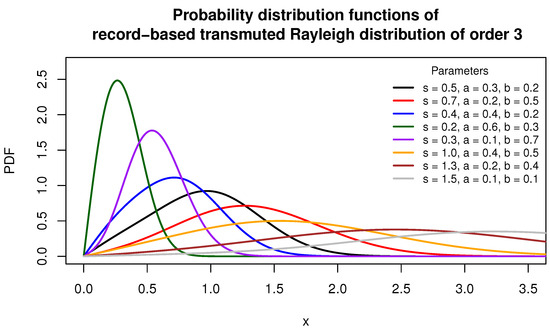
Figure 1.
The PDFs of various rbt-Rayleigh distributions.
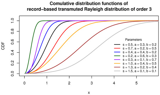
Figure 2.
The CDFs of various rbt-Rayleigh- distributions.
The hazard rate function (HRF) of rbt-Rayleigh distribution is given by:
Since the baseline distribution in our model is the Rayleigh distribution, whose hazard function is strictly increasing (i.e., the Rayleigh distribution is IFR), it is of interest to examine whether this property is preserved under the record-based transmuted transformation of order 3.
This question has been addressed and rigorously proven by Balakrishnan and He (see Section 3.3 in [22]), who showed that the resulting distribution retains the IFR property of the baseline if the transformation parameters satisfy the condition
Hence, in our case, the proposed distribution is IFR whenever this condition holds.
3. Quantile Function
The cumulative distribution function (CDF) of the rbt–Rayleigh distribution is given by
To compute the quantile function , we must solve the nonlinear equation
which does not admit a closed-form solution for general values of a, b, and . Therefore, the quantile function is computed numerically.
To address this, we implemented a root-finding algorithm in R that solves the equation above for a given probability level . The corresponding R code is provided below and can be used to generate a full quantile table or compute specific quantiles such as the median or quartiles.
R Code for Computing the Quantile Function of the rbt–Rayleigh Distribution
Listing 1 presents the R code that numerically computes the quantile function of the rbt–Rayleigh distribution by solving the nonlinear equation.
| Listing 1. R code for computing the quantile function of the rbt–Rayleigh distribution. |
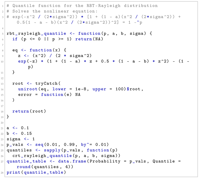 |
Table 1 reports the quantile values of the rbt–Rayleigh distribution for selected probabilities, while Figure 3 illustrates the quantile function for , using parameters , , and .

Table 1.
Quantile values of the rbt-R distribution for selected probabilities . Parameters: , , .
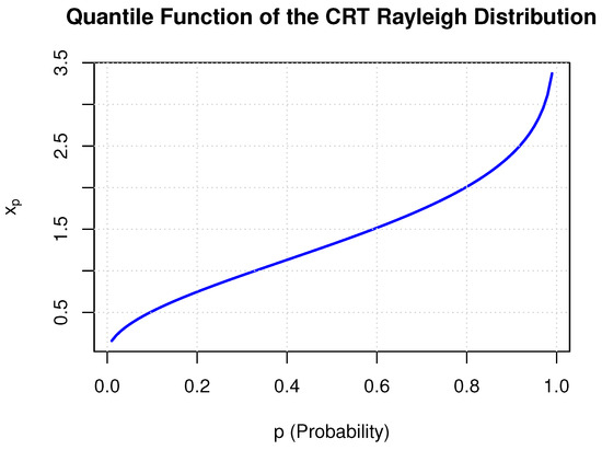
Figure 3.
The plot of the quantile function of the rbt-Rayleigh distribution for , with parameters , , and . The function was numerically evaluated using the inverse of the cumulative distribution function and visualized in R.
4. Moments
Theorem 1.
If , then the moment of X is given by:
Specifically, the mean and variance are obtained as follows:
Proof.
The result follows by applying the integral identity given in (7). □
Throughout the remainder of the manuscript, we denote the r-th raw moment of the distribution by . This notation is used for expressing skewness and kurtosis in terms of the central moments.
Theorem 2.
If , then the moment generating function of X, denoted by , is given by:
Proof.
By definition,
Since
one obtains
For any finite interval , the function is continuous on and hence bounded. Therefore, there exists a constant such that
Hence,
Since
the series converges uniformly on by the Weierstrass M-test. Each term is continuous on . By the Uniform Convergence Theorem for the Riemann integral, one obtains
The function is integrable on and tends to zero faster than any polynomial as . Hence, letting yields
From the explicit expression of the moments one obtains
□
The values presented in Table 2 and Table 3 correspond to the mean and variance of the random variable computed for selected combinations of the parameters a, b, and .
Table 2.
Mean values of X for selected combinations of a, b, and .
Table 3.
Variance values of X for selected combinations of a, b, and .
5. Skewness and Kurtosis
In addition to the first two moments, which characterize the location and dispersion of a distribution, the third and fourth central moments provide insight into its shape. These are commonly summarized by the coefficients of skewness and kurtosis.
The coefficient of skewness measures the asymmetry of the distribution around its mean. A positive skewness indicates a longer right tail, whereas a negative value implies a heavier left tail. For a random variable X, the skewness is defined as:
The coefficient of kurtosis, on the other hand, quantifies the heaviness of the tails and the sharpness of the peak relative to a normal distribution. It is given by:
For the proposed rbt-Rayleigh distribution, explicit expressions for the moments have been derived in Theorem 1. These can be directly substituted into the formulas above to compute the skewness and kurtosis as functions of the parameters a, b, and .
6. Harmonic Mean
Theorem 3.
If , then the harmonic mean of X, defined as , is given by:
Proof.
We compute the expected value of the reciprocal:
Using the Gaussian integrals:
we conclude that:
□
7. Mean Deviations
The mean deviation about the mean and the mean deviation about the median are defined by:
where is the mean, and M denotes the median of the distribution.
Theorem 4.
For the rbt-R distribution, the mean deviations and are given by:
and
8. Entropy
Entropy measures provide a formal means of quantifying the uncertainty inherent in probability distributions. Among them, Shannon entropy is the most widely used, while the Rényi entropy [25], a parametric generalization, offers a broader framework for analyzing distributional characteristics [26].
Let X be a continuous random variable with probability density function . The Rényi entropy of order , is defined by
Theorem 5.
Let . The Rényi entropy of order α for the rbt-R distribution is given by:
Proof.
Applying the binomial expansion yields
For any finite interval , the function is continuous and hence bounded on . Therefore, there exists a constant such that
Since
converges absolutely, by the Weierstrass M-test, the double series converges uniformly on . Each term in the sum is continuous on . By the Uniform Convergence Theorem for the Riemann integral, one obtains
The function tends to zero faster than any polynomial as . Thus, taking the limit yields
Applying the integral identity
gives
Hence,
□
9. Order Statistics
Let denote the order statistics from an i.i.d. sample drawn from a continuous distribution with probability density function (PDF) and cumulative distribution function (CDF) .
The PDF of the order statistic is given by:
If , then
When , we obtain the PDF of the smallest observation in the sample:
For the rbt-R distribution, this becomes:
When , we obtain the PDF of the largest observation in the sample:
For the rbt-R distribution, this becomes
10. Maximum Likelihood Estimation
Let denote a random sample drawn from the record-based transmuted Rayleigh distribution of order 3, with parameters and , subject to the constraint .
The likelihood function corresponding to this sample is given by:
Taking logarithms, we obtain the log-likelihood function:
To estimate , we differentiate with respect to each parameter and set the score equations to zero:
In general, this nonlinear system has no closed-form solution, and numerical methods such as the Broyden–Fletcher–Goldfarb–Shanno (BFGS) algorithm or Newton–Raphson are employed to maximize the log-likelihood subject to the parameter constraints.
Under standard regularity conditions, the maximum likelihood estimator is asymptotically normal. Specifically:
where , and is the Fisher information matrix:
To confirm this result, we verify that the usual regularity conditions are satisfied:
- Interior Point: The true parameter lies in the interior of the space .
- Differentiability: The log-likelihood is continuously differentiable on for all .
- Identifiability: The model is identifiable since each parameter combination yields a distinct density.
- Fisher Information: The matrix exists and is positive definite.
- Finite Expectations: Expectations involving the first and second derivatives are finite due to the exponential tail of the density.
To clarify notation, the gradient and the Hessian are given by:
The explicit expressions for the second-order partial derivatives used in this Hessian matrix are provided in Appendix A.
The observed information matrix is:
Its inverse gives the estimated variance–covariance matrix:
Approximate confidence intervals are constructed as:
where is the standard normal quantile.
For reporting purposes:
This formulation allows practitioners to assess parameter uncertainty and construct valid confidence intervals. Empirical examples using this procedure are provided in the following sections.
11. Application to Real Data
To evaluate the practical performance of the proposed record-based transmuted Rayleigh distribution of order 3 (rbtR), we fitted it to four real-world datasets. For comparison purposes, we also fitted the Rayleigh distribution (R), the transmuted Rayleigh distribution (T-R), the generalized Rayleigh distribution (G-R) as introduced in Surles and Padgett [27], and the transmuted generalized Rayleigh distribution (TGR). Model comparison was conducted using multiple goodness-of-fit criteria, namely the Akaike Information Criterion (AIC), the corrected Akaike Information Criterion (AICc), the Bayesian Information Criterion (BIC), and the Kolmogorov–Smirnov distance (KS). Additionally, overlay plots of the estimated probability density functions and cumulative distribution functions were provided to facilitate a visual assessment of fit quality.
11.1. Dataset 1: Nicotine Yields (FTC, 1994)
Source: Federal Trade Commission (FTC), Cigarette Yields Report, 1994 (EconDataUS).
The first dataset analyzed in this study relates to nicotine yield levels reported in 1994 by the U.S. Federal Trade Commission (FTC) in their widely referenced document titled “Tar, Nicotine, and Carbon Monoxide of the Smoke of 1206 Varieties of Domestic Cigarettes”. This report remains a central source for researchers studying chemical content in cigarettes, and it is freely available online: https://www.ftc.gov/system/files/documents/reports/report-tar-nicotine-carbon-monoxide-smoke-1206-varieties-domestic-cigarettes-year-1994/tarandnico.pdf (accessed on 10 January 2025).
According to the FTC’s documentation, nicotine yields were measured using the Cambridge Filter Method—an approach the agency has endorsed since 1967 to ensure consistency across cigarette brands. The measurements, expressed in milligrams per cigarette, were rounded to the nearest 0.1 mg.
Data were collected from various manufacturers across more than 50 locations in the United States. The report includes results from the five dominant companies at the time: Philip Morris, R. J. Reynolds, Lorillard, Brown & Williamson, and Liggett Group. In the case of lesser-known brands, data were often submitted directly by the manufacturers, following FTC guidelines.
In addition to yield values, the report outlines sample collection protocols and standard smoking conditions, such as the 23 mm smoked butt length, which contribute to the reproducibility of the data. Previous studies by Sloan and Sublett [28] and Schultz and Spears [29] further support the accuracy of the laboratory techniques applied.
This dataset serves as a useful illustration for examining how well the proposed rbt-Rayleigh distribution performs in practice. Descriptive statistics are provided in Table 4, while parameter estimates and model selection criteria—obtained via maximum likelihood estimation—are summarized in Table 5 and Table 6.
Table 4.
Descriptive statistics for variable X (N = 346).
Table 5.
Parameter estimates and log-likelihood for Rayleigh-type models for Dataset 1.
Table 6.
Goodness-of-fit measures for Dataset 1.
A histogram of the observed nicotine yields is presented in Figure 4, while the empirical versus fitted CDFs are displayed in Figure 5. The log-likelihood contour plot, with fixed at its MLE, is shown in Figure 6.
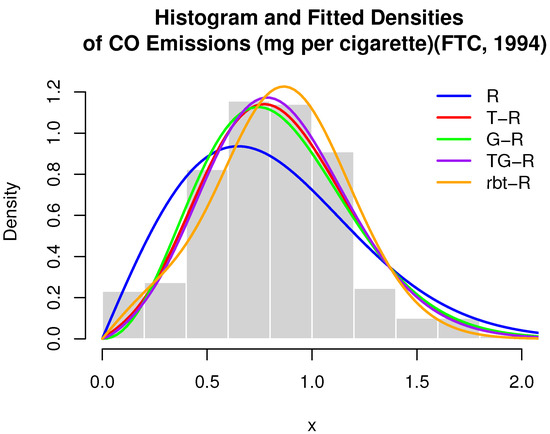
Figure 4.
Nicotine yields (mg per cigarette).
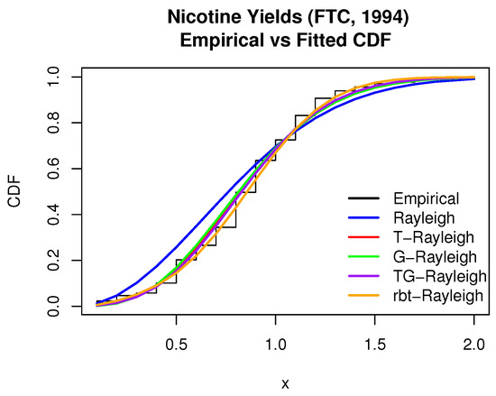
Figure 5.
Empirical vs. fitted CDF—nicotine yields.
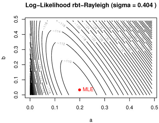
Figure 6.
Log-likelihood contour—nicotine yields ( fixed at MLE).
The observed Fisher information matrix (i.e., the negative of the Hessian matrix of the log-likelihood evaluated at the MLEs) under the rbt-Rayleigh distribution is estimated as:
The inverse of this matrix, denoted by , provides the estimated variance–covariance matrix of the maximum likelihood estimators (MLEs):
Based on this, the approximate 95% confidence intervals for the parameters , a, and b are computed as:
11.2. Dataset 2: Carbon Monoxide Emissions (FTC, 2007)
Source: U.S. Federal Trade Commission (FTC), “Nicotine, Tar, and CO Content of Domestic Cigarettes in 2007—Regular Brands, sorted by nicotine, tar, and CO.” Available at: https://www.econdataus.com/cigrs.html, accessed on 23 June 2025.
This dataset reports carbon monoxide (CO) emissions per cigarette, measured in milligrams, as published by the FTC in 2007. The data were extracted from the publicly available table titled “Regular Brands, sorted by CO”, which presents standardized yield values for a wide range of domestic cigarette brands.
Measurements were obtained using the Cambridge Filter Method, a standardized laboratory technique recommended by the FTC to ensure comparability across brands. CO emission values are rounded to the nearest 0.1 mg and cover major tobacco manufacturers in the U.S. market.
The distribution of CO emissions exhibits moderate right skew due to a small number of high-emission brands. The proposed rbt-Rayleigh model fits the observed data closely, capturing the distributional shape more effectively than alternative models. Among the models evaluated, it achieves the lowest Kolmogorov–Smirnov (KS) distance (0.037), indicating superior goodness-of-fit.
Descriptive statistics for CO emissions are presented in Table 7. Parameter estimates and log-likelihood values for the considered models are reported in Table 8, while goodness-of-fit criteria are summarized in Table 9. A histogram of the observed CO emission values is shown in Figure 7, the empirical versus fitted CDFs are displayed in Figure 8, and the log-likelihood contour plot—with fixed at its MLE—is provided in Figure 9.
Table 7.
Descriptive statistics for variable X (N = 816).
Table 8.
Parameter estimates and log-likelihood for CO emission models.
Table 9.
Goodness-of-fit measures for CO emission models.
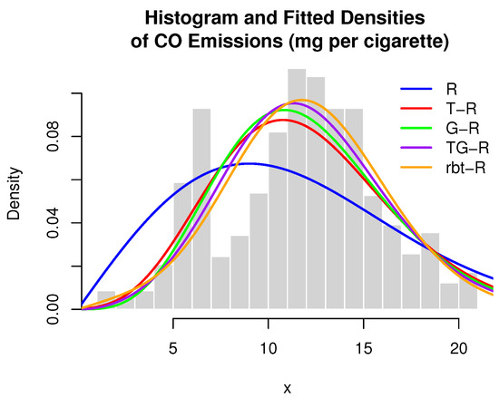
Figure 7.
CO emissions (mg per cigarette).
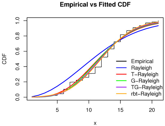
Figure 8.
Empirical vs. fitted CDF—CO emissions.
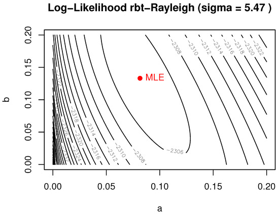
Figure 9.
Log-likelihood contour—CO emissions ( fixed at MLE).
The estimated variance–covariance matrix of the MLEs under the rbt-R distribution is given by:
11.3. Dataset 3: Carbon-Fibre Breaking Stress (50 mm Gauge)
The carbon-fibre breaking stress values analyzed in this study correspond to tensile strength measurements (in GPa) collected from fibres with a gauge length of 50 mm, as reported by Lishamol and Jiju [30]. These measurements were obtained under controlled conditions from production samples, in accordance with standard testing procedures used to ensure that the fibres meet the necessary strength requirements for composite applications.
Of particular interest is the lower tail of the strength distribution—especially the first percentile—as reductions in this region may signal declining fibre quality and compromise the structural integrity of the resulting composite material.
This dataset serves as the third case study in our analysis (see Table 10). Descriptive statistics are visualized in Figure 10, and the empirical versus fitted CDFs are displayed in Figure 11. The proposed three-parameter rbt-Rayleigh distribution demonstrates a superior fit, achieving the lowest AIC, AICc, BIC, and KS values across competing models (Table 11 and Table 12). The corresponding log-likelihood surface (Figure 12) confirms the presence of a unique optimal solution.
Table 10.
Breaking stress values (in GPa) for Dataset 3.
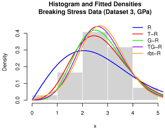
Figure 10.
Breaking stress (Dataset 3, GPa).
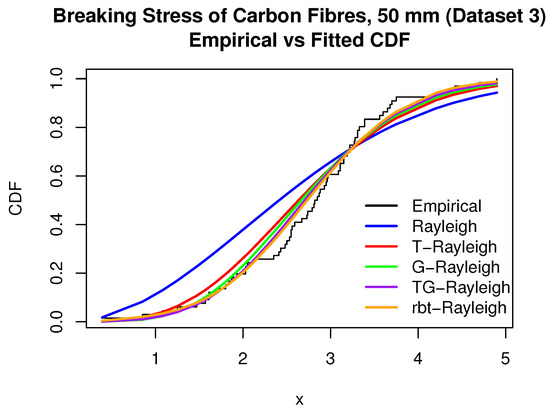
Figure 11.
Empirical vs. fitted CDF—breaking stress (Dataset 3).
Table 11.
Parameter estimates and log-likelihood for Dataset 3.
Table 12.
Goodness-of-fit measures for Dataset 3.
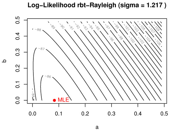
Figure 12.
Log-likelihood contour—breaking stress (Dataset 3) ( fixed).
The estimated variance–covariance matrix of the MLEs under the rbt-R distribution is given by:
11.4. Dataset 4: Carbon-Fibre Breaking Stress (20 mm Gauge)
This dataset consists of tensile strength measurements for carbon fibres tested at a gauge length of 20 mm, as reported by Badar and Priest [31]. The strength values, expressed in gigapascals (GPa), were obtained under controlled laboratory conditions.
Using a shorter gauge length than that in Dataset 3 reduces the likelihood of encountering surface flaws in the tested segment. As a result, the measured strengths in this dataset tend to be slightly higher.
This distinction in testing setup provides a good opportunity to examine how the proposed rbt-Rayleigh distribution performs when the data come from a similar material but under different conditions. The observed breaking stress values for this dataset are presented in Table 13.
Table 13.
Observed breaking stress values (GPa) for Dataset 4 (carbon fibre, 20 mm gauge length).
A summary of the descriptive statistics is given in Table 14, while parameter estimates and goodness-of-fit results appear in Table 15 and Table 16. Visual diagnostics are shown in Figure 13, Figure 14 and Figure 15. Once again, the rbt-R model provides the best fit, outperforming all four competing distributions across all evaluation metrics (Table 15 and Table 16). This superiority is further supported by graphical diagnostics shown in Figure 13, Figure 14 and Figure 15.
Table 14.
Descriptive statistics for Dataset 4 ().
Table 15.
Parameter estimates and log-likelihood for Rayleigh-type distributions—Dataset 4.
Table 16.
Goodness-of-fit measures for Rayleigh-type distributions—Dataset 4.
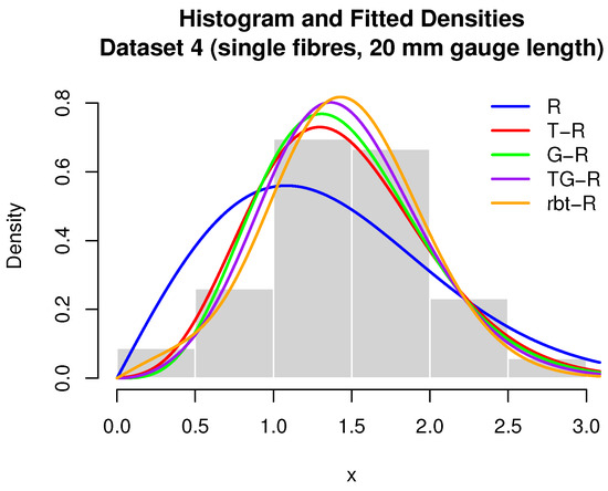
Figure 13.
Breaking stress (Dataset 4, GPa).
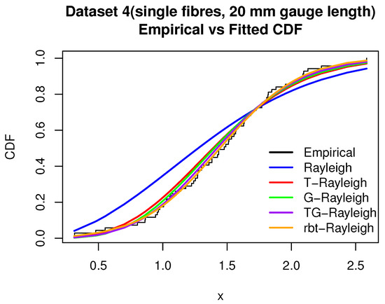
Figure 14.
Empirical vs. fitted CDF—breaking stress (Dataset 4).
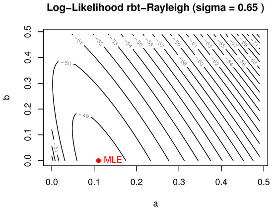
Figure 15.
Log-likelihood contour—breaking stress (Dataset 4) ( fixed).
The estimated variance–covariance matrix of the MLEs under the rbt-R distribution is given by:
11.5. Summary of Results Across Datasets
The rbt-R distribution provides the best overall fit according to AIC, AICc, BIC, and KS criteria.
12. Random Sampling via Inverse Transform and Newton–Raphson
To investigate the finite-sample properties of the rbt-R maximum likelihood estimators, synthetic data are generated using a combination of the inverse-transform method and Newton–Raphson root-finding. The procedure is as follows:
- Fix the true parameter vector , set the sample size n, and choose an initial value (we use the Rayleigh quantile approximation below).
- For each , draw .
- Computewhich provides a Rayleigh-based initial guess.
- Solve the equationiteratively viawhere f and F denote the rbt-R density and CDF, respectively. Iteration stops when or after 50 steps, whichever occurs first.
- Upon convergence, set . Repeat steps 2–5 for all to obtain the simulated sample .
13. Monte Carlo Experiment
We evaluated the performance of the estimator at the true parameter values , in the sample sizes
For each n, we perform independent replications. In each replication:
- Generate a sample of size n using the inverse-Newton method described above;
- Obtain the MLEs via constrained optimization (L–BFGS–B);
- Store the estimated triplet.
For each parameter , we compute:
The results by sample size are presented in Table A1 and Table A2; both tables are provided in the Appendix B.
14. Conclusions
In this work, we present a new three-parameter extension of the classical Rayleigh distribution by applying the record-based transmuted-G (RBT-G) distribution of order 3, originally introduced by Balakrishnan and He. The resulting model, referred to as the rbt-Rayleigh distribution of order 3, offers increased flexibility to capture skewness and heavy-tailed behavior while retaining analytical tractability. Several analytical properties of the proposed distribution are derived, including the r-th raw and central moments, the harmonic mean, Shannon entropy, the quantile function, and the order statistics. The model parameters are estimated using the maximum likelihood method, implemented via numerical optimization in the R programming environment.
To assess the model’s performance, the rbt-Rayleigh distribution is applied to four empirical datasets: two related to cigarette composition (nicotine content and carbon monoxide emissions), and two concerning carbon-fibre tensile strength. A comparative analysis is conducted using standard goodness-of-fit criteria: Akaike Information Criterion (AIC), corrected Akaike Information Criterion (AICc), Bayesian Information Criterion (BIC), and the Kolmogorov–Smirnov (KS) statistic. In all cases, the rbt-Rayleigh model demonstrates a superior fit relative to the classical Rayleigh, transmuted Rayleigh, generalized Rayleigh, and transmuted generalized Rayleigh distributions.
Funding
This research received no external funding.
Data Availability Statement
Datasets 1 and 2 are publicly available from the EconDataUS repository https://econdataus.com/smoke.html, (accessed 10 May 2025). Datasets 3 and 4 are included within the main text of the paper.
Conflicts of Interest
The author declares no conflicts of interest.
Appendix A. Second-Order Derivatives of the Log-Likelihood
The second-order partial derivatives of the log-likelihood function are given below:
where
Appendix B. Simulation Study
Table A1.
Empirical means of the MLEs for various n.
Table A1.
Empirical means of the MLEs for various n.
| n | ||||||
|---|---|---|---|---|---|---|
| 10 | 0.30 | 0.40 | 2.00 | 0.2776 | 0.2315 | 1.9304 |
| 20 | 0.30 | 0.40 | 2.00 | 0.2910 | 0.2766 | 1.9527 |
| 30 | 0.30 | 0.40 | 2.00 | 0.3053 | 0.2947 | 1.9701 |
| 40 | 0.30 | 0.40 | 2.00 | 0.3052 | 0.3238 | 1.9809 |
| 50 | 0.30 | 0.40 | 2.00 | 0.3113 | 0.3318 | 1.9909 |
| 60 | 0.30 | 0.40 | 2.00 | 0.3166 | 0.3291 | 1.9955 |
| 70 | 0.30 | 0.40 | 2.00 | 0.3158 | 0.3283 | 1.9948 |
| 80 | 0.30 | 0.40 | 2.00 | 0.3191 | 0.3231 | 1.9957 |
| 90 | 0.30 | 0.40 | 2.00 | 0.3152 | 0.3378 | 1.9988 |
| 100 | 0.30 | 0.40 | 2.00 | 0.3160 | 0.3417 | 2.0004 |
| 110 | 0.30 | 0.40 | 2.00 | 0.3171 | 0.3441 | 2.0024 |
| 120 | 0.30 | 0.40 | 2.00 | 0.3154 | 0.3472 | 2.0010 |
| 130 | 0.30 | 0.40 | 2.00 | 0.3148 | 0.3521 | 2.0043 |
| 140 | 0.30 | 0.40 | 2.00 | 0.3150 | 0.3542 | 2.0043 |
| 150 | 0.30 | 0.40 | 2.00 | 0.3157 | 0.3563 | 2.0062 |
| 160 | 0.30 | 0.40 | 2.00 | 0.3172 | 0.3549 | 2.0070 |
| 170 | 0.30 | 0.40 | 2.00 | 0.3165 | 0.3586 | 2.0087 |
| 180 | 0.30 | 0.40 | 2.00 | 0.3176 | 0.3548 | 2.0072 |
| 190 | 0.30 | 0.40 | 2.00 | 0.3177 | 0.3536 | 2.0063 |
| 200 | 0.30 | 0.40 | 2.00 | 0.3185 | 0.3559 | 2.0079 |
| 210 | 0.30 | 0.40 | 2.00 | 0.3182 | 0.3564 | 2.0071 |
| 220 | 0.30 | 0.40 | 2.00 | 0.3175 | 0.3581 | 2.0072 |
| 230 | 0.30 | 0.40 | 2.00 | 0.3182 | 0.3588 | 2.0076 |
| 240 | 0.30 | 0.40 | 2.00 | 0.3169 | 0.3602 | 2.0072 |
| 250 | 0.30 | 0.40 | 2.00 | 0.3170 | 0.3630 | 2.0087 |
| 260 | 0.30 | 0.40 | 2.00 | 0.3168 | 0.3669 | 2.0109 |
| 270 | 0.30 | 0.40 | 2.00 | 0.3158 | 0.3707 | 2.0114 |
| 280 | 0.30 | 0.40 | 2.00 | 0.3161 | 0.3685 | 2.0105 |
| 290 | 0.30 | 0.40 | 2.00 | 0.3149 | 0.3680 | 2.0092 |
| 300 | 0.30 | 0.40 | 2.00 | 0.3148 | 0.3706 | 2.0105 |
| 310 | 0.30 | 0.40 | 2.00 | 0.3149 | 0.3715 | 2.0110 |
| 320 | 0.30 | 0.40 | 2.00 | 0.3143 | 0.3720 | 2.0108 |
| 330 | 0.30 | 0.40 | 2.00 | 0.3136 | 0.3740 | 2.0110 |
| 340 | 0.30 | 0.40 | 2.00 | 0.3146 | 0.3745 | 2.0122 |
| 350 | 0.30 | 0.40 | 2.00 | 0.3143 | 0.3753 | 2.0116 |
| 360 | 0.30 | 0.40 | 2.00 | 0.3142 | 0.3744 | 2.0111 |
| 370 | 0.30 | 0.40 | 2.00 | 0.3142 | 0.3743 | 2.0112 |
| 380 | 0.30 | 0.40 | 2.00 | 0.3140 | 0.3734 | 2.0107 |
| 390 | 0.30 | 0.40 | 2.00 | 0.3136 | 0.3740 | 2.0103 |
| 400 | 0.30 | 0.40 | 2.00 | 0.3138 | 0.3741 | 2.0103 |
| 410 | 0.30 | 0.40 | 2.00 | 0.3135 | 0.3750 | 2.0101 |
| 420 | 0.30 | 0.40 | 2.00 | 0.3133 | 0.3748 | 2.0096 |
| 430 | 0.30 | 0.40 | 2.00 | 0.3127 | 0.3771 | 2.0102 |
| 440 | 0.30 | 0.40 | 2.00 | 0.3125 | 0.3805 | 2.0116 |
| 450 | 0.30 | 0.40 | 2.00 | 0.3125 | 0.3805 | 2.0114 |
| 460 | 0.30 | 0.40 | 2.00 | 0.3128 | 0.3814 | 2.0123 |
| 470 | 0.30 | 0.40 | 2.00 | 0.3131 | 0.3821 | 2.0133 |
| 480 | 0.30 | 0.40 | 2.00 | 0.3131 | 0.3823 | 2.0132 |
| 490 | 0.30 | 0.40 | 2.00 | 0.3130 | 0.3841 | 2.0135 |
| 500 | 0.30 | 0.40 | 2.00 | 0.3130 | 0.3838 | 2.0132 |
Table A2.
Empirical MSEs of the MLEs for various n.
Table A2.
Empirical MSEs of the MLEs for various n.
| n | ||||||
|---|---|---|---|---|---|---|
| 10 | 0.30 | 0.40 | 2.00 | 0.07478 | 0.15215 | 0.12203 |
| 20 | 0.30 | 0.40 | 2.00 | 0.05540 | 0.13649 | 0.07197 |
| 30 | 0.30 | 0.40 | 2.00 | 0.04825 | 0.12766 | 0.05825 |
| 40 | 0.30 | 0.40 | 2.00 | 0.03807 | 0.12022 | 0.04425 |
| 50 | 0.30 | 0.40 | 2.00 | 0.03370 | 0.11448 | 0.04117 |
| 60 | 0.30 | 0.40 | 2.00 | 0.02918 | 0.11037 | 0.03931 |
| 70 | 0.30 | 0.40 | 2.00 | 0.02488 | 0.10290 | 0.03669 |
| 80 | 0.30 | 0.40 | 2.00 | 0.02082 | 0.09507 | 0.03437 |
| 90 | 0.30 | 0.40 | 2.00 | 0.01795 | 0.09336 | 0.03080 |
| 100 | 0.30 | 0.40 | 2.00 | 0.01656 | 0.09035 | 0.02928 |
| 110 | 0.30 | 0.40 | 2.00 | 0.01625 | 0.08864 | 0.02910 |
| 120 | 0.30 | 0.40 | 2.00 | 0.01422 | 0.08482 | 0.02623 |
| 130 | 0.30 | 0.40 | 2.00 | 0.01334 | 0.08412 | 0.02624 |
| 140 | 0.30 | 0.40 | 2.00 | 0.01190 | 0.08094 | 0.02453 |
| 150 | 0.30 | 0.40 | 2.00 | 0.01177 | 0.07878 | 0.02403 |
| 160 | 0.30 | 0.40 | 2.00 | 0.01097 | 0.07734 | 0.02290 |
| 170 | 0.30 | 0.40 | 2.00 | 0.01001 | 0.07396 | 0.02204 |
| 180 | 0.30 | 0.40 | 2.00 | 0.00985 | 0.07195 | 0.02145 |
| 190 | 0.30 | 0.40 | 2.00 | 0.00974 | 0.07043 | 0.02107 |
| 200 | 0.30 | 0.40 | 2.00 | 0.00936 | 0.06925 | 0.02096 |
| 210 | 0.30 | 0.40 | 2.00 | 0.00903 | 0.06693 | 0.02026 |
| 220 | 0.30 | 0.40 | 2.00 | 0.00858 | 0.06485 | 0.01939 |
| 230 | 0.30 | 0.40 | 2.00 | 0.00844 | 0.06370 | 0.01925 |
| 240 | 0.30 | 0.40 | 2.00 | 0.00814 | 0.06286 | 0.01891 |
| 250 | 0.30 | 0.40 | 2.00 | 0.00787 | 0.06234 | 0.01902 |
| 260 | 0.30 | 0.40 | 2.00 | 0.00749 | 0.06179 | 0.01858 |
| 270 | 0.30 | 0.40 | 2.00 | 0.00706 | 0.06006 | 0.01811 |
| 280 | 0.30 | 0.40 | 2.00 | 0.00677 | 0.05880 | 0.01824 |
| 290 | 0.30 | 0.40 | 2.00 | 0.00647 | 0.05755 | 0.01751 |
| 300 | 0.30 | 0.40 | 2.00 | 0.00614 | 0.05711 | 0.01723 |
| 310 | 0.30 | 0.40 | 2.00 | 0.00584 | 0.05656 | 0.01689 |
| 320 | 0.30 | 0.40 | 2.00 | 0.00562 | 0.05625 | 0.01653 |
| 330 | 0.30 | 0.40 | 2.00 | 0.00538 | 0.05562 | 0.01625 |
| 340 | 0.30 | 0.40 | 2.00 | 0.00532 | 0.05532 | 0.01625 |
| 350 | 0.30 | 0.40 | 2.00 | 0.00511 | 0.05436 | 0.01559 |
| 360 | 0.30 | 0.40 | 2.00 | 0.00505 | 0.05305 | 0.01543 |
| 370 | 0.30 | 0.40 | 2.00 | 0.00501 | 0.05193 | 0.01530 |
| 380 | 0.30 | 0.40 | 2.00 | 0.00492 | 0.05084 | 0.01499 |
| 390 | 0.30 | 0.40 | 2.00 | 0.00480 | 0.05048 | 0.01474 |
| 400 | 0.30 | 0.40 | 2.00 | 0.00470 | 0.04909 | 0.01454 |
| 410 | 0.30 | 0.40 | 2.00 | 0.00457 | 0.04835 | 0.01435 |
| 420 | 0.30 | 0.40 | 2.00 | 0.00439 | 0.04816 | 0.01412 |
| 430 | 0.30 | 0.40 | 2.00 | 0.00424 | 0.04810 | 0.01405 |
| 440 | 0.30 | 0.40 | 2.00 | 0.00417 | 0.04736 | 0.01388 |
| 450 | 0.30 | 0.40 | 2.00 | 0.00410 | 0.04731 | 0.01370 |
| 460 | 0.30 | 0.40 | 2.00 | 0.00401 | 0.04727 | 0.01368 |
| 470 | 0.30 | 0.40 | 2.00 | 0.00397 | 0.04656 | 0.01359 |
| 480 | 0.30 | 0.40 | 2.00 | 0.00386 | 0.04581 | 0.01332 |
| 490 | 0.30 | 0.40 | 2.00 | 0.00379 | 0.04539 | 0.01314 |
| 500 | 0.30 | 0.40 | 2.00 | 0.00374 | 0.04449 | 0.01311 |
References
- Shaw, W.T.; Buckley, I.R. The Alchemy of Probability Distributions: Beyond Gram-Charlier and Cornish-Fisher Expansions, and Skew-Normal or Kurtotic-Normal Distributions. UCL Discovery Repository. 2007. Available online: https://library.wolfram.com/infocenter/Articles/6670/alchemy.pdf (accessed on 15 February 2025).
- Merovci, F.; Alizadeh, M.; Hamedani, G.G. Another generalized transmuted family of distributions: Properties and applications. Austrian J. Stat. 2016, 45, 71–93. [Google Scholar] [CrossRef]
- Moolath, G.B.; Jayakumar, K. T-transmuted X family of distributions. Statistica 2017, 77, 251–276. [Google Scholar]
- Granzotto, D.C.T.; Louzada, F.; Balakrishnan, N. Cubic rank transmuted distributions: Inferential issues and applications. J. Stat. Comput. Simul. 2017, 87, 2760–2778. [Google Scholar] [CrossRef]
- Rahman, M.M.; Gemeay, A.M.; Khan, M.A.I.; Meraou, M.A.; Bakr, M.E.; Muse, A.H.; Balogun, O.S. A new modified cubic transmuted-G family of distributions: Properties and different methods of estimation with applications to real-life data. AIP Adv. 2023, 13, 095025. [Google Scholar] [CrossRef]
- Rayleigh, L. On the stability, or instability, of certain fluid motions. Proc. Lond. Math. Soc. 1880, 9, 57–70. [Google Scholar] [CrossRef]
- Siddiqui, M.M. Some problems connected with Rayleigh distributions. J. Res. Natl. Bur. Stand. D 1962, 66, 167. [Google Scholar] [CrossRef]
- Siddiqui, M.M. Statistical inference for Rayleigh distributions. J. Res. Natl. Bur. Stand. Sec. D 1964, 68, 1007. [Google Scholar] [CrossRef]
- Vickers, J.W. A Parameter Estimation Technique for the Generalized Rayleigh-Rician Distribution and Laha’s Bessel Distribution; PN: Fort Belvoir, VA, USA, 1976. [Google Scholar]
- Beckmann, P. Rayleigh distribution and its generalizations. Radio Sci. J. Res. NBS/USNC-URSI 1964, 68, 927–932. [Google Scholar] [CrossRef]
- Kundu, D.; Raqab, M.Z. Generalized Rayleigh distribution: Different methods of estimations. Comput. Stat. Data Anal. 2005, 49, 187–200. [Google Scholar] [CrossRef]
- Voda, V.G. A new generalization of Rayleigh distribution. Reliab. Theory Appl. 2007, 2, 47–56. [Google Scholar]
- Abd Elfattah, A.M.; Hassan, A.S.; Ziedan, D.M. Efficiency of maximum likelihood estimators under different censored sampling schemes for Rayleigh distribution. Interstat 2006, 1, 1–16. [Google Scholar]
- Merovci, F. Transmuted Rayleigh distribution. Austrian J. Stat. 2013, 42, 21–31. [Google Scholar] [CrossRef]
- Merovci, F. Transmuted generalized Rayleigh distribution. J. Stat. Appl. Probab. 2014, 3, 9. [Google Scholar] [CrossRef]
- Mir, A.A.; Ahmad, S.P. A New Extended Rayleigh Distribution with Applications of COVID-19 Data. Austrian J. Stat. 2025, 54, 69–84. [Google Scholar] [CrossRef]
- Rivera, P.A.; Barranco-Chamorro, I.; Gallardo, D.I.; Gómez, H.W. Scale Mixture of Rayleigh Distribution. Mathematics 2020, 8, 1842. [Google Scholar] [CrossRef]
- Vodă, V.G. Inferential procedures on a generalized Rayleigh variate. I. Apl. Mat. 1976, 21, 395–412. [Google Scholar] [CrossRef]
- Santoro, K.I.; Gallardo, D.I.; Venegas, O.; Cortés, I.E.; Gómez, H.W. A Heavy-Tailed Distribution Based on the Lomax–Rayleigh Distribution with Applications to Medical Data. Mathematics 2023, 11, 4626. [Google Scholar] [CrossRef]
- Haj Ahmad, H.; Ramadan, D.A.; Almetwally, E.M. Evaluating the discrete generalized Rayleigh distribution: Statistical inferences and applications to real data analysis. Mathematics 2024, 12, 183. [Google Scholar] [CrossRef]
- Dong, Y.; Gui, W. Reliability Estimation in Stress Strength for Generalized Rayleigh Distribution Using a Lower Record Ranked Set Sampling Scheme. Mathematics 2024, 12, 1650. [Google Scholar] [CrossRef]
- Balakrishnan, N.; He, M. A record-based transmuted family of distributions. In Advances in Statistics-Theory and Applications: Honoring the Contributions of Barry C. Arnold in Statistical Science; Springer: Cham, Switzerland, 2021; pp. 3–24. [Google Scholar]
- Gradshteyn, I.S.; Ryzhik, I.M. Table of Integrals, Series, and Products; Academic Press: Cambridge, MA, USA, 2014. [Google Scholar]
- Rudin, W. Principles of Mathematical Analysis, 3rd ed.; McGraw-Hill: New York, NY, USA, 1976. [Google Scholar]
- Rényi, A. On measures of entropy and information. In Proceedings of the Fourth Berkeley Symposium on Mathematical Statistics and Probability, Volume 1: Contributions to the Theory of Statistics; University of California Press: Berkeley, CA, USA, 1961; Volume 4, pp. 547–562. [Google Scholar]
- Shannon, C.E. A mathematical theory of communication. Bell Syst. Tech. J. 1948, 27, 379–423. [Google Scholar] [CrossRef]
- Surles, J.G.; Padgett, W.J. Inference for reliability and stress strength for a scaled Burr type X distribution. Lifetime Data Anal. 2001, 7, 187–200. [Google Scholar] [CrossRef] [PubMed]
- Sloan, C.H.; Sublett, B.J. Determination of methyl nitrite in cigarette smoke. Tob. Sci. 1967, 11, 21–24. [Google Scholar]
- Schultz, F.J.; Spears, A.W. Determination of moisture in total particulate matter. Tob. Sci. 1966, 10, 75–76. [Google Scholar]
- Lishamol, T.; Jiju, G. A generalized Rayleigh distribution and its application. Biom. Biostat. Int. J. 2019, 8, 139–143. [Google Scholar]
- Bader, M.G.; Priest, A.M. Statistical aspects of fibre and bundle strength in hybrid composites. In Progress in Science and Engineering of Composites; The Japan Society for Composite Materials: Tokyo, Japan, 1982; pp. 1129–1136. [Google Scholar]
Disclaimer/Publisher’s Note: The statements, opinions and data contained in all publications are solely those of the individual author(s) and contributor(s) and not of MDPI and/or the editor(s). MDPI and/or the editor(s) disclaim responsibility for any injury to people or property resulting from any ideas, methods, instructions or products referred to in the content. |
© 2025 by the author. Licensee MDPI, Basel, Switzerland. This article is an open access article distributed under the terms and conditions of the Creative Commons Attribution (CC BY) license (https://creativecommons.org/licenses/by/4.0/).