Decarbonizing China’s Express Freight Market Using High-Speed Rail Services and Carbon Taxes: A Bi-Level Optimization Approach

Abstract

This study explores the potential for reducing CO₂ emissions in China’s express freight sector by promoting a modal shift from air and road transport to high-speed rail (HSR) through the implementation of a carbon tax policy. A bi-level optimization model is employed to analyze the decision-making processes of three key stakeholders: the government, HSR operators, and shippers. The government aims to maximize consumer surplus while reducing CO₂ emissions through a carbon tax policy; HSR operators seek to maximize transportation profit; and shippers select the most efficient transportation mode based on cost and service considerations. A solution algorithm combining particle swarm optimization, the CPLEX solver, and a custom convergence procedure is designed to solve the bi-level programming model and determine the optimal carbon tax rate. The findings from the Beijing–Shanghai corridor case study indicate that a well-designed carbon tax policy, when integrated with robust HSR services, can effectively encourage a modal shift towards HSR. The extent of emission reduction is influenced by both the capacity of HSR infrastructure and the stringency of the carbon tax policy. This research highlights the importance of addressing asymmetries in transportation mode preferences and market demands. The integration of carbon tax policies with HSR services not only mitigates emissions but also promotes greater symmetry and efficiency within the transportation network.

1. Introduction

The transportation sector is a significant contributor to global CO₂ emissions. Modal shifts toward greener freight modes are critical for energy conservation and emission-reduction targets [1]. Modal shifts reallocate freight between transport modes. This shift is fundamentally driven by changes in mode choice and user preferences, which are highly sensitive to factors such as user characteristics, model attributes, infrastructure, and regulatory policies [2].

Governments have recognized the urgency of transitioning freight transport from road to more sustainable modes such as railways and inland waterways. For instance, in 2018, China set an ambitious target to increase national railway freight volume by 30% by 2020 compared to 2017, although the actual growth achieved was 21%. Similarly, the European Union established goals in 2013 to shift 30% of long-distance cargo transport from road to greener modes by 2030 and an additional 20% by 2050. Achieving these targets, however, faces challenges such as rail service capacity limitations and shipper preferences. Thus, it is imperative for governments to collaborate with green transportation companies to realize modal shift and CO₂ emission reduction objectives.

The rapid growth of e-commerce has significantly increased the demand for express cargo transportation. Between 2020 and 2024, China’s express-delivery volume rose from 83 billion to 175 billion parcels [3]. Express parcel transportation contributes to approximately 14.3% of the carbon emissions within the transportation sector in China [4]. The current express freight market is predominantly served by air and road freight. High-speed rail (HSR), with its speed and punctuality, presents a promising alternative. Over the past decade, China’s HSR network has expanded rapidly to nearly 40,000 km, connecting over 75% of the country’s cities at regional and national levels. This extensive network has the potential to play a significant role in decarbonizing the express freight transport system. Bi et al. [5] suggested that countries like China, France, Germany, and Japan should leverage the unused space in HSR passenger trains for express package delivery. This practice not only boosts HSR operating income but also alleviates pressure on highway and air express transportation.

By addressing the inherent asymmetries in the freight market, such as the dominance of air and road transport and the underutilization of HSR, the study provides valuable insights into achieving sustainable development in the express freight market. This research focuses on developing a carbon tax policy designed to encourage a shift toward more environmentally friendly freight modes. Given that air transportation’s greenhouse gas emissions per shipment are nearly an order of magnitude higher than those of other modes [6], this study aims to offer novel insights for governments to formulate effective decarbonization policies. By modeling the system to determine optimal policies, the research proposes a model that maximizes consumer welfare while considering shippers’ mode choices and the capacity limitations of green transportation modes. Furthermore, this study provides HSR freight operators with optimal service design decisions. The model optimizes cargo flow allocation under four distinct HSR freight organization modes and determines the service frequency for each mode. As a result of the modal shift, an increase in HSR freight profit is anticipated. This study addresses a modeling problem involving three key stakeholders—government, carriers, and shippers—using a bi-level optimization approach to capture the interdependencies of their actions.

The remainder of this paper is organized as follows. Section 2 reviews the relevant literature. Section 3 presents the methodology, covering model formulation and algorithm design. Section 4 undertakes numerical experiments to determine the optimal carbon tax. Section 5 offers an in-depth discussion. Finally, Section 6 concludes the research.

2. Literature Review

Existing studies propose the Avoid–Improve–Shift strategy for freight decarbonization. This involves avoiding unnecessary transport, enhancing energy efficiency via technology, and developing clean energy. However, decarbonizing freight by cutting transport demand is difficult due to its strong link with economic growth. Energy efficiency improvements may fall short of expectations due to the rebound effect. Clean energy development also demands substantial infrastructure investment. Modal shift is crucial for reducing greenhouse gas emissions [7], reducing particulate matter emissions [8], and alleviating truck transportation overload [9]. Most studies address bulk-cargo modal shifts (coal, ore) from road to rail, but neglect markets with high value-added and time–efficiency demands such as fresh products and precision instruments.

As shown in Table 1, the government can drive freight modal shift through the implementation of policy instruments, with particular emphasis on subsidies and tax policies. While subsidy policies operate on the principle of providing incentives, carbon tax policies adopt a penalty-based approach. This distinction enables carbon tax policies to achieve their objectives without incurring an increase in government fiscal expenditure. In the absence of policy intervention, the negative environmental costs stemming from transportation activities, including air pollution, noise, and traffic congestion, are typically neither borne by shippers or carriers nor do they influence transportation mode selection. The internalization of external costs ensures that these detrimental factors are incorporated into the decision-making process regarding transportation mode choice. This practice contributes to enhancing equity among transportation users.

Although the imposition of taxation policies renders all transportation modes more costly, clean transportation modes, characterized by lower external costs, gain a competitive edge. Nevertheless, the potential rise in product prices resulting from these policies may lead to a decline in consumer welfare. To address this issue, strategies such as tax revenue recycling schemes have been employed to mitigate the adverse effects of carbon taxes. Zhou et al. [10] developed a computable general equilibrium model to simulate the impacts of carbon taxes on China’s transportation industry and designed two tax recycling schemes aimed at achieving government revenue neutrality. Qiu et al. [11] proposed a bi-level optimization model to investigate airline passenger carbon taxes, which encompasses both the levy of carbon taxes and competitive tax rebates for airlines. Their research suggested that airlines should transfer a portion of carbon-related costs to passengers.

Table 1. Research on promoting modal shift by policy tools.

Reference	Measures to Promote Modal Shift	Model
Wang et al. [12]	Carbon tax on shippers	Two-stage Stackelberg gaming model
Bouchery et al. [13]	Control total carbon emissions	Multi-objective optimization
Tao et al. [14]	Fix subsidy to shippers	Random coefficient logit model
Choi et al. [15]	Containerization and taxes	System dynamics model
Kundu and Sheu [16]	Subsidy to shippers	Sequential game-theoretic model
Chen et al. [17]	Joint tax–subsidy policy	Mathematical program with complementarity constraints
Guo et al. [18]	Pricing, road construction, increasing railway service level, and railway subsidy	System dynamic modeling and Monte Carlo simulation
Nassar et al. [19]	Fiscal and regulatory measures and infrastructure investments	System Dynamics approach
Takman and Gonzalez-Aregall [20]	Subsidies and regulations	Ex post evaluations
Masone et al. [7]	Incentive schemes	Simulate shipper’s mode choice behavior
Shen et al. [21]	Pricing of railway	Mixed logit model

Table 1. Research on promoting modal shift by policy tools.

Reference	Measures to Promote Modal Shift	Model
Wang et al. [12]	Carbon tax on shippers	Two-stage Stackelberg gaming model
Bouchery et al. [13]	Control total carbon emissions	Multi-objective optimization
Tao et al. [14]	Fix subsidy to shippers	Random coefficient logit model
Choi et al. [15]	Containerization and taxes	System dynamics model
Kundu and Sheu [16]	Subsidy to shippers	Sequential game-theoretic model
Chen et al. [17]	Joint tax–subsidy policy	Mathematical program with complementarity constraints
Guo et al. [18]	Pricing, road construction, increasing railway service level, and railway subsidy	System dynamic modeling and Monte Carlo simulation
Nassar et al. [19]	Fiscal and regulatory measures and infrastructure investments	System Dynamics approach
Takman and Gonzalez-Aregall [20]	Subsidies and regulations	Ex post evaluations
Masone et al. [7]	Incentive schemes	Simulate shipper’s mode choice behavior
Shen et al. [21]	Pricing of railway	Mixed logit model

The feasibility of HSR freight has been demonstrated across technological, economic, and environmental dimensions. Hoffrichter et al. [22] compared the energy consumption and CO₂ emissions of railway and road vehicles, revealing that even in high-speed operation mode, shifting to rail can cut CO₂ emissions. Research on HSR freight predominantly concerns dedicated HSR freight trains. Jia et al. [23] optimized the number and departure time of freight trains on the Beijing–Xi’an HSR via a bi-level optimization model, the upper level of which maximized railway industry profits while the lower level applied user equilibrium principles to optimize cargo flow distribution. Yu et al. [24] and Yu et al. [25] designed a freight operation plan and a train diagram for China’s Harbin–Dalian HSR. Recent studies have furthered HSR freight operations exploration. Li et al. [26] investigated the development of reliable HSR freight train timetables with buffer times to balance efficiency and punctuality. Li et al. [27] addressed large-scale HSR freight train rescheduling, presenting an efficient algorithm for complex networks. Wang et al. [28] proposed a combined HSR and crowd–courier system for parcel delivery, optimizing rail freight allocation and road courier routing. Zhang et al. [29] focused on cargo distribution in high-speed freight trains to prevent wind-induced overturning, employing dynamics modeling and prediction. Li et al. [30] handled HSR line planning for passenger and freight services, developing a multi-objective model and hybrid algorithm. These studies have improved HSR freight operations’ reliability, efficiency, and safety through novel optimization models and algorithms.

This paper makes the following key contributions to the field:

(1) Carbon Tax Policy Design. This policy helps to internalize the external environmental costs associated with transportation, encouraging a shift towards more sustainable freight modes and contributing to decarbonization goals; (2) Bi-level Optimization Model. The paper introduces a bi-level mixed-integer optimization model that effectively combines HSR freight operation planning, carbon tax optimization, and transportation mode choice. This model accounts for the capacity limitations of HSR freight, ensuring that the proposed policies are practical and effective; (3) Algorithm Development. Given that the bi-level programming model is a complex NP-hard problem, the paper develops a solution procedure by integrating particle swarm optimization (PSO) with the CPLEX toolbox. The designed algorithm convergence strategy efficiently addresses the challenges of carbon tax policy decision-making, offering a useful tool for policymakers; (4) Practical insights. Through a case study of the Beijing–Shanghai corridor, the study demonstrates the potential of modal shifts and carbon tax policies in reducing emissions in the express freight market.

3. Methodology

3.1. Problem Description

The decision-making process for promoting freight modal shift involves three key stakeholders: policymakers (government), transportation suppliers (carriers), and transportation demanders (shippers). A bi-level model captures stakeholder interactions. In the express freight market, the three primary transportation modes are HSR, road, and air, with their environmental friendliness defined by CO₂ emissions per unit turnover, decreasing in the order of HSR, road, and air.

As shown in Figure 1, in the upper level, the government aims to optimize the carbon tax policy to reduce CO₂ emissions while minimizing the impact on consumer surplus across the entire express freight system. The carbon tax policy influences shippers by encouraging them to choose more environmentally friendly transportation modes. In the lower level, the model considers that HSR freight services might not fully satisfy shippers’ demands. The actual supply of HSR freight is determined by its transportation capacity and the goal of maximizing operational profit. Any unmet demand for HSR is assumed to be fulfilled by road and air transport. The CO₂ emissions from the freight system are calculated based on the market share of each mode and fed back to the government. Through multiple iterations between the upper and lower levels, the government can determine the appropriate carbon tax policy. Section 3.2, Section 3.3, Section 3.4 and Section 3.5 detail the establishment of this model.

The carbon tax is calculated based on the volume of goods transported, the distance traveled, and CO₂ emission factors, then multiplied by the tax rate per unit of CO₂ emissions. This mechanism aims to internalize the environmental costs of transportation, thereby incentivizing shippers and operators to reduce CO₂ emissions and promote sustainable freight transport. By increasing the cost of polluting modes, the tax encourages shippers to select more environmentally friendly alternatives. HSR operators may gain a competitive advantage from this policy, making HSR more attractive compared to road and air transport. However, they must also strategize on optimizing services to accommodate potential increases in freight demand resulting from modal shifts.

Table 2. Notations.

Sets:
$\mathbb{S}$	set of transportation nodes. $\mathbb{S}=\left\{1,\dots ,s,\dots ,S\right\}$
$\mathbb{L}$	set of origin-destination (OD) pairs. $\mathbb{L}=\left\{ij:i,j\in \mathbb{S}\right\}$
$\mathbb{N}$	set of express freight demand types, differentiated by their distinct transportation time requirements. $\mathbb{N}=\left\{n_1,n_2\right\}$
$\mathbb{M}$	set of freight modes in the express transport market. $\mathbb{M}=\left\{HSR,road,air\right\}$
$ℝ$	set of HSR freight organization modes. $ℝ=\left\{r_1,r_2,r_3,r_4\right\}$
$\mathbb{T}$	set of HSR passenger train classifications capable of meeting freight demand. $\mathbb{T}=\left\{t_1,t_2,t_3\right\}$
Parameters:
$p_{ij,n}^m$	freight rate for demand $n\in \mathbb{N}$ between OD $ij\in \mathbb{L}$ transported by mode $m\in \mathbb{M}$ (CNY/kg)
$c_{fix}^r$	fixed operating cost of HSR mode $r\in ℝ$ (CNY)
$c_l^r$	distance-related cost of HSR mode $r\in ℝ$ (CNY/km)
$l_{ij}^m$	transportation distance for goods transported by mode $m\in \mathbb{M}$ between OD $ij\in \mathbb{L}$ (km)
$c_q^r$	volume-related cost of HSR mode $r\in ℝ$ (CNY/kg)
$t_{ij,n}^m$	transportation time of demand $n\in \mathbb{N}$ between OD $ij\in \mathbb{L}$ transported by mode $m\in \mathbb{M}$ (h)
$t_{way}^{ij,m}$	en-route transportation time for goods transported by mode $m\in \mathbb{M}$ between OD $ij\in \mathbb{L}$ (h)
$t_{door}^m$	fixed station-to-door delivery time of mode $m\in \mathbb{M}$ (h)
$t_{wait}^{m,n}$	waiting time for demand $n\in \mathbb{N}$ transported by mode $m\in \mathbb{M}$ (h)
$v^m$	average transportation speed of mode $m\in \mathbb{M}$ (km/h)
$T_n$	delivery time limit for demand $n\in \mathbb{N}$ (h)
${\xi }_{ij}^{fre}$	maximum service frequency of HSR freight trains between OD $ij\in \mathbb{L}$
${\xi }_{ij,t}^{pas}$	maximum service frequency of HSR passenger trains with classification $t\in \mathbb{T}$ between OD $ij\in \mathbb{L}$
$N_r$	maximum freight capacity of a single train in HSR mode $r\in ℝ$ (kg)
$Q_{ij,n}$	total demand of $n\in \mathbb{N}$ between OD $ij\in \mathbb{L}$ (kg)
$Q_{ij,n}^m$	demand of $n\in \mathbb{N}$ between OD $ij\in \mathbb{L}$ that selects mode $m\in \mathbb{M}$ (kg)
${\mathrm{Pr}}_{ij,n}^m$	probability of demand of $n\in \mathbb{N}$ between OD $ij\in \mathbb{L}$ selecting mode $m\in \mathbb{M}$
$U_{ij,n}^m$	the perceived utility of demand $n\in \mathbb{N}$ for mode $m\in \mathbb{M}$ between OD $ij\in \mathbb{L}$
$V_{ij,n}^m$	deterministic part of the utility
${\epsilon }_{ij,n}^m$	random component of the utility
$o^m$	punctuality rate of mode $m\in \mathbb{M}$ (%)
$s^m$	safety of mode $m\in \mathbb{M}$ (%)
$d^m$	cargo damage rate of mode $m\in \mathbb{M}$ (%)
${\sigma }^m$	unit CO2 emissions of mode $m\in \mathbb{M}$ (tCO2/kg-km)
$e_{ij}^m$	carbon tax per unit of goods transported by mode $m\in \mathbb{M}$ between OD $ij\in \mathbb{L}$ (CNY/kg)
${\alpha }_1,\dots ,{\alpha }_5$	weight of each attribute in the utility function
${\lambda }_{\min },{\lambda }_{\max }$	minimum and maximum allowable values for the carbon tax rate (CNY/tCO2)
Decision variables:
$q_{ij,n}^r$	freight volume of demand $n\in \mathbb{N}$ between OD $ij\in \mathbb{L}$ transported by HSR mode $r\in ℝ$ (kg)
$q_{ij}^r$	freight volume transported by HSR mode $r\in ℝ$ for OD $ij\in \mathbb{L}$ (kg)
${\psi }_{ij}^r$	required service frequency for HSR mode $r\in ℝ$ between OD $ij\in \mathbb{L}$
$q_{ij,n}^{r,t}$	freight volume of demand $n\in \mathbb{N}$ between OD $ij\in \mathbb{L}$ transported by HSR mode $r\in ℝ$ using trains classified as $t\in \mathbb{T}$
${\psi }_{ij}^{r,t}$	required service frequency for HSR mode $r\in ℝ$ using trains classified as $t\in \mathbb{T}$
$q_{ij,n}^m$	freight volume of demand $n\in \mathbb{N}$ between OD $ij\in \mathbb{L}$ transported by mode $m\in \mathbb{M}$ (kg)
$\lambda$	carbon tax rate (CNY/tCO2)

summarizes variables and parameters used in the modelling.

3.2. HSR Operator: Profit Maximization

Define the set of HSR freight organization modes as $ℝ=\left\{r_1,r_2,r_3,r_4\right\}$. The elements in the set represent the following four patterns in sequence [31]:

(r₁) The inspecting train: this is the first non-passenger train each day tasked with testing the safety of HSR tracks; (r₂) Piggyback pattern: this pattern utilizes the residual luggage storage space on HSR passenger trains for goods transportation; (r₃) Normal HSR passenger trainsets: in these HSR passenger trains, several carriages are specifically allocated for express freight transportation; (r₄) Dedicated HSR freight train: this pattern enables complete segregation of freight and passenger transportation.

This section aims to conduct the assignment of freight demands across the HSR modes to determine the actual freight volume of HSR freight.

The HSR freight operator aims to maximize transportation profit: revenue (Equation (1)) minus cost (Equation (2)). The revenue is obtained by multiplying the HSR freight rate by the freight volume. The cost comprises three components: fixed transportation costs, variable costs that depend on transportation distance, and variable costs that depend on freight volume. Equation (3) calculates the total freight volume of OD ij transported by HSR mode r.

$$I(\mathit{q})={\displaystyle \sum _{ij\in \mathbb{L}}{\displaystyle \sum _{n\in \mathbb{N}}{\displaystyle \sum _{r\in ℝ}{p}_{ij,n}^{HSR}{q}_{ij,n}^r}}}$$

(1)

$$C(\mathit{\psi },\mathit{q})={\displaystyle \sum _{r\in ℝ}{\displaystyle \sum _{ij\in \mathbb{L}}\left(c_{fix}^r{\psi }_{ij}^r+c_l^r{l}_{ij}^{HSR}{\psi }_{ij}^r+c_q^r{q}_{ij}^r\right)}}$$

(2)

$$q_{ij}^r={\displaystyle \sum _{n\in \mathbb{N}}{q}_{ij,n}^r},\forall ij\in \mathbb{L},r\in ℝ$$

(3)

The objective of the transportation profit maximization problem is presented in Equation (4), subject to the following constraints (i)–(iii).

$$\max \hspace{1em}I(\mathit{q})-C(\mathit{\psi },\mathit{q})$$

(4)

(i) Constraint of transportation time

In the express freight market, there are two primary types of transportation demand:

• Type one consists of transportation demands that require delivery within 12 h (n = n₁).
• Type two consists of transportation demands that require delivery within 24 h (n = n₂).

Moreover, demand type n₁ is dispatched after 10:00 on the day of arrival, while demand type n₂ is dispatched after 18:00 on the same day. Accordingly, the required train operation time ranges for demands n₁ and n₂ are $10:00~22:00-t_{door}^m$ and $18:00~18:{00}^{+1}-t_{door}^m$, respectively.

The following three components of transportation time are considered: en-route transportation time, station waiting time, and station-to-door time. For freight demand $n$ of OD $ij$, the transportation time required by mode m is calculated using Equation (5). The en-route transportation time is derived from the ratio of the transportation distance to the average speed (Equation (6)). Denote the delivery time limit for freight demand n of OD ij as $T_{ij,n}$ (Equation (7)). Consequently, the delivery time constraint for HSR transportation is presented in Equation (8).

$$t_{ij,n}^m=t_{way}^{ij,m}+t_{door}^m+t_{wait}^{m,n},\forall ij\in \mathbb{L},n\in \mathbb{N},m\in \mathbb{M}$$

(5)

$$t_{way}^{ij,m}={\displaystyle \frac{l_{ij}^m}{v^m}},\forall ij\in \mathbb{L},m\in \mathbb{M}$$

(6)

$$T_n=\left\{\begin{array}{l}12,n=n_1\\ 24,n=n_2\end{array}\right.$$

(7)

$$t_{ij,n}^{HSR}\le T_n,\forall ij\in \mathbb{L},n\in \mathbb{N}$$

(8)

(ii) Constraint of load capacity

The HSR inspecting train (r₁) operates daily starting at 04:00 and is unable to meet the demand for n₁ (Equation (9)). It can run at most once per day (Equation (10)). The dedicated freight train mode (r₄) is entirely separate from passenger operations and is constrained by the maximum number of HSR freight trains permitted (Equation (11)).

$$q_{ij,n_1}^{r_1}=0,\forall ij\in \mathbb{L}$$

(9)

$${\psi }_{ij}^{r_1}\le 1,\forall ij\in \mathbb{L}$$

(10)

$${\psi }_{ij}^{r_4}\le {\xi }_{ij}^{fre},\forall ij\in \mathbb{L}$$

(11)

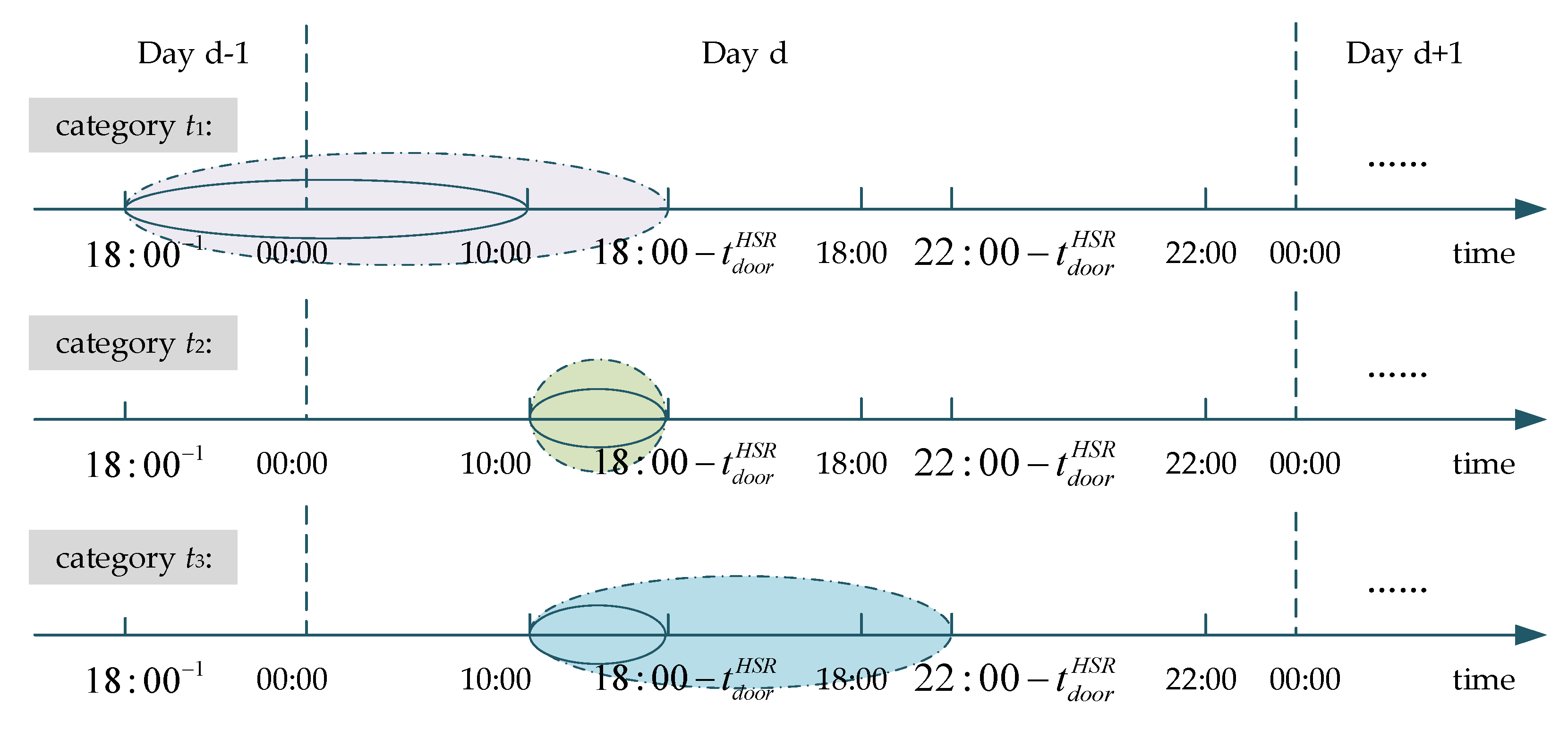
The HSR freight modes r₂ and r₃ depend on existing HSR passenger trains. According to Figure 2, passenger trains that can meet modes r₂ and r₃ are divided into three categories. The solid ellipse in Figure 2 represents the range of passenger train departure time, and the dashed ellipse represents the range of passenger train arrival time. It can be seen that trains in category t₁ can only meet the demand n₂, trains in category t₃ can only meet the demand n₁, and trains in category t₂ can satisfy both demands n₁ and n₂. Thus, Equations (12)–(14) hold.

$$0\le q_{ij,n}^{r,t_2}\le q_{ij,n}^r,\forall ij\in \mathbb{L},n\in \mathbb{N},r\in \left\{r_2,r_3\right\}$$

(12)

$$q_{ij,n_2}^r=q_{ij,n_2}^{r,t_1}+q_{ij,n_2}^{r,t_2},\forall ij\in \mathbb{L},r\in \left\{r_2,r_3\right\}$$

(13)

$$q_{ij,n_1}^r=q_{ij,n_1}^{r,t_3}+q_{ij,n_1}^{r,t_2},\forall ij\in \mathbb{L},r\in \left\{r_2,r_3\right\}$$

(14)

Equation (15) indicates that the required service frequency of HSR modes r₂ and r₃, utilizing passenger trains in category t, cannot exceed the maximum service frequency of trains in category t. For HSR modes r₂ and r₃, the required service frequency for transporting goods of OD ij is the sum of service frequencies across categories t₁ to t₃ (Equation (16)). Equations (17)–(20) specify that the freight volume allocated to each HSR mode cannot exceed the available freight capacity of trains in each category. The capacity is determined by multiplying the maximum capacity per HSR train by the train service frequency.

$${\displaystyle \sum _{r\in \left\{r_2,r_3\right\}}{\psi }_{ij}^{r,t}}\le {\xi }_{ij,t}^{pas},\forall ij\in \mathbb{L},t\in \mathbb{T}$$

(15)

$${\psi }_{ij}^r={\displaystyle \sum _{t\in \mathbb{T}}{\psi }_{ij}^{r,t}},\forall ij\in \mathbb{L},r\in \left\{r_2,r_3\right\}$$

(16)

$$q_{ij,n_2}^{r,t_1}\le N_r{\psi }_{ij}^{r,t_1},\forall ij\in \mathbb{L},r\in \left\{r_2,r_3\right\}$$

(17)

$${\displaystyle \sum _{n\in \mathbb{N}}{q}_{ij,n}^{r,t_2}}\le N_r{\psi }_{ij}^{r,t_2},\forall ij\in \mathbb{L},r\in \left\{r_2,r_3\right\}$$

(18)

$$q_{ij,n_1}^{r,t_3}\le N_r{\psi }_{ij}^{r,t_3},\forall ij\in \mathbb{L},r\in \left\{r_2,r_3\right\}$$

(19)

$$q_{ij}^r\le N_r{\psi }_{ij}^r,\forall ij\in \mathbb{L},r\in \left\{r_1,r_4\right\}$$

(20)

(iii) Constraint of freight volume

The non-negativity of the freight volume is enforced by Equation (21). As shown in Equation (22), the HSR freight demand is the product of the total demand and the probability of selecting HSR, where the probability ${\mathrm{Pr}}_{ij,n}^{HSR}$ is obtained from the shipper choice behavior analysis in Section 3.3. Equation (23) ensures that the actual freight volume managed by HSR remains within the bounds of demand.

$$q_{ij,n}^r\ge 0,\forall ij\in \mathbb{L},n\in \mathbb{N},r\in ℝ$$

(21)

$$Q_{ij,n}^{HSR}=Q_{ij,n}{\mathrm{Pr}}_{ij,n}^{HSR},\forall ij\in \mathbb{L},n\in \mathbb{N}$$

(22)

$${\displaystyle \sum _{r\in ℝ}{q}_{ij,n}^r}\le Q_{ij,n}^{HSR},\forall ij\in \mathbb{L},n\in \mathbb{N}$$

(23)

3.3. Shipper: Mode Choice

The Multinomial Logit (MNL) model serves as a widely employed discrete choice framework for analyzing shippers’ transportation mode decisions. Extensive prior research has established methodologies for calculating consumer surplus within this framework, thereby supporting the articulation of government policy objectives. According to the MNL model, the utility $U_{ij,n}^m$ comprises observable deterministic components $V_{ij,n}^m$ and unobservable stochastic components ${\epsilon }_{ij,n}^m$, as presented in Equation (24).

$$U_{ij,n}^m=V_{ij,n}^m+{\epsilon }_{ij,n}^m,\forall ij\in \mathbb{L},n\in \mathbb{N},m\in \mathbb{M}$$

(24)

Assume that the random terms of the utility (${\epsilon }_{ij,n}^m$) are independently and identically distributed (i.i.d.) and follow the Gumbel distribution. When each shipper selects the mode with the highest utility among all available options, this selection process results in the well-known MNL formula presented in Equation (25). Let ${\mathrm{Pr}}_{ij,n}^m$ denote the probability of choosing mode m.

$${\mathrm{Pr}}_{ij,n}^m={\displaystyle \frac{\exp \left(V_{ij,n}^m\right)}{{\displaystyle \sum _{m^{\prime }\in \mathbb{M}}\exp \left(V_{ij,n}^{m^{\prime }}\right)}}},\forall ij\in \mathbb{L},n\in \mathbb{N},m\in \mathbb{M}$$

(25)

Economy, timeliness, reliability, safety, and environmental externality are chosen as the attributes of $V_{ij,n}^m$.

(1)

Economy

The economic attribute is directly related to the freight rates of various transportation modes ($p_{ij,n}^m$).

(2)

Timeliness

The timeliness is expressed by the transportation time ($t_{ij,n}^m$).

(3)

Reliability

The reliability of various transportation modes can be expressed by their punctuality rates ($o^m$).

(4)

Safety

The safety ($s^m$) of various transportation modes can be expressed by their cargo damage rates ($d^m$).

$$s^m=1-d^m,\forall m\in \mathbb{M}$$

(26)

(5)

Environmental externality

The negative environmental externalities are expressed in terms of the carbon tax levied per unit of freight volume.

$$e_{ij}^m=\lambda {\sigma }^m{l}_{ij}^m,\forall ij\in \mathbb{L},m\in \mathbb{M}$$

(27)

The deterministic utility of mode m based on these attributes is given by Equation (28). The parameters $\left\{{\alpha }_1,{\alpha }_2,\dots ,{\alpha }_5\right\}$ can be estimated using maximum likelihood estimation.

$$V_{ij,n}^m={\alpha }_1{p}_{ij,n}^m+{\alpha }_2{t}_{ij,n}^m+{\alpha }_3{o}^m+{\alpha }_4{s}^m+{\alpha }_5{e}_{ij}^m,\forall ij\in \mathbb{L},n\in \mathbb{N},m\in \mathbb{M}$$

(28)

3.4. Government: Decarbonization and Consumer Surplus Maximization

In the market of transportation demand $n$ between OD $ij$, the expected consumer surplus is given in Equation (29) [32]:

$$E(C{S}_{ij,n})=E[{\displaystyle \frac{1}{{\beta }^{ij,n}}}\underset{m\in \mathbb{M}}{\max }{U}_{ij,n}^m]=E[{\displaystyle \frac{1}{\left|{\alpha }_1\right|}}\underset{m\in \mathbb{M}}{\max }{U}_{ij,n}^m],\forall ij\in \mathbb{L},n\in \mathbb{N}$$

(29)

where ${\beta }^{ij,n}$ denotes the marginal utility of money, which corresponds to the absolute value of the coefficient of $p_{ij,n}^m$ in the MNL model [33,34].

The expected consumer surplus can be modeled as the logsum of the observable utility after monetization, as shown in Equation (30).

$$E(C{S}_{ij,n})={\displaystyle \frac{1}{\left|{\alpha }_1\right|}}\ln ({\displaystyle \sum _{m\in \mathbb{M}}\exp (V_{ij,n}^m}))+C,\forall ij\in \mathbb{L},n\in \mathbb{N}$$

(30)

The total consumer surplus within the transportation corridor is presented in Equation (31), where C represents a constant. The government’s objective is to maximize consumer surplus (Equation (32)). Additionally, the decision variable—carbon tax rate $\lambda$—must be within a specified range (Equation (33)).

$$CS(\mathit{\lambda })={\displaystyle \sum _{ij\in \mathbb{L}}{\displaystyle \sum _{n\in \mathbb{N}}{Q}_{ij,n}E(C{S}_{ij,n})}} ={\displaystyle \sum _{ij\in \mathbb{L}}{\displaystyle \sum _{n\in \mathbb{N}}{Q}_{ij,n}\frac{1}{\left|{\alpha }_1\right|}\ln ({\displaystyle \sum _{m\in \mathbb{M}}\exp (V_{ij,n}^m}))}}+{\displaystyle \sum _{ij\in \mathbb{L}}{\displaystyle \sum _{n\in \mathbb{N}}{Q}_{ij,n}C}}$$

(31)

$$\max CS(\mathit{\lambda })$$

(32)

$${\lambda }_{\min }\le \lambda \le {\lambda }_{\max }$$

(33)

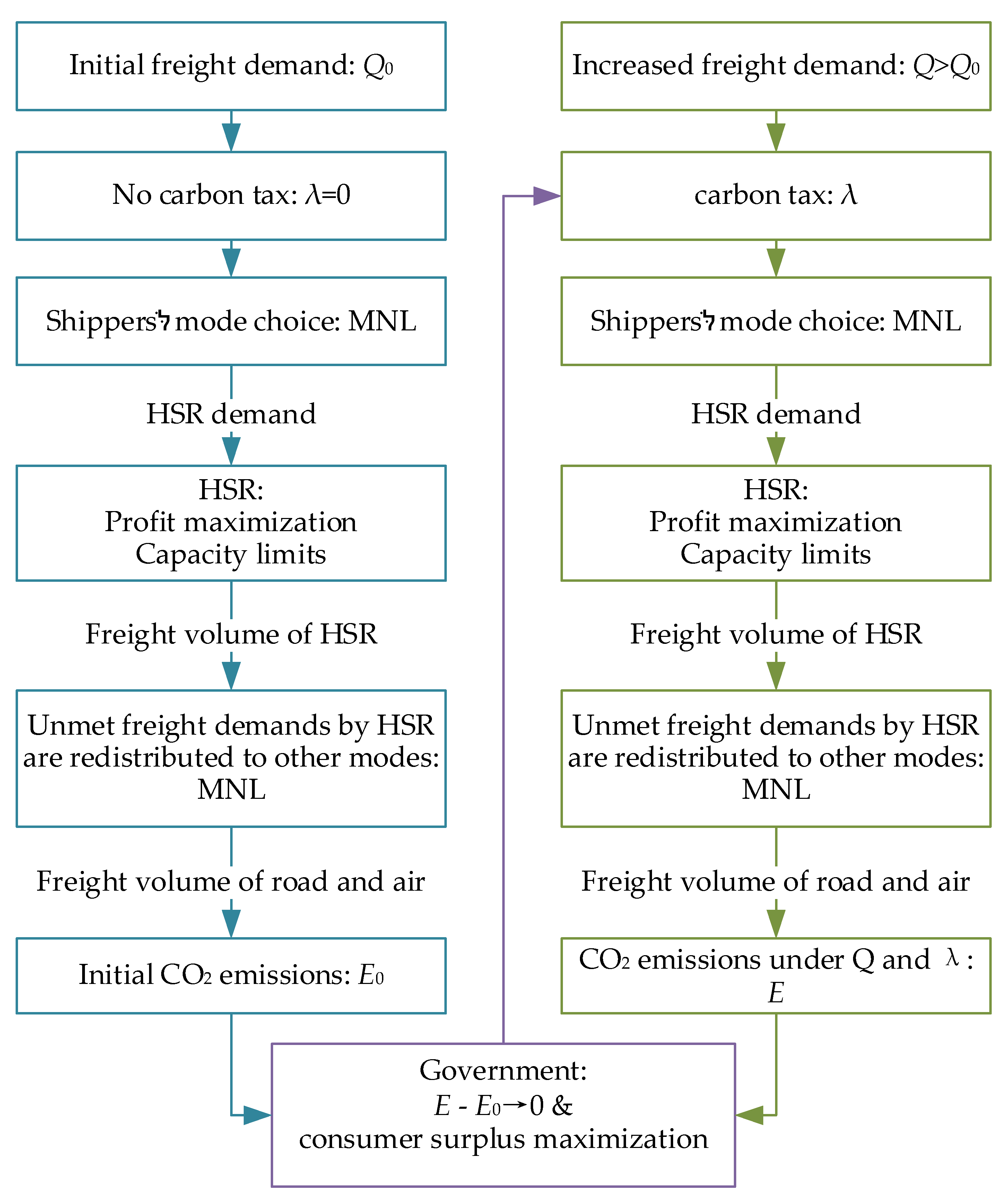
The decarbonization objective of this study is to eliminate the CO₂ emissions resulting from the growth in express freight demand, which aligns with the global pursuit of net-zero CO₂ emissions [35]. Figure 3 illustrates the detailed decarbonization process. The HSR freight demand $Q_{ij,n}^{HSR}$ is derived from the shipper’s mode choice model. Subsequently, the actual HSR supply $q_{ij,n}^{HSR}$ is determined by the profit-maximization model outlined in Section 3.2. Given the HSR transportation capacity constraints, any unmet freight demands $Q_{ij,n}^{HSR}-q_{ij,n}^{HSR}$ are diverted to other viable modes (road and air) in accordance with the MNL model (Equation (34)). It is assumed that these alternative modes can fully accommodate the diverted demands. Ultimately, the total CO₂ emissions of the freight system are calculated as Equation (35).

$$q_{ij,n}^m=Q_{ij,n}^m=(Q_{ij,n}-q_{ij,n}^{HSR}){\mathrm{Pr}}_{ij,n}^m,\forall ij\in \mathbb{L},n\in \mathbb{N},m\in \left\{road,air\right\}$$

(34)

$$E(\mathit{Q},\lambda )={\displaystyle \sum _{ij\in \mathbb{L}}{\displaystyle \sum _{n\in \mathbb{N}}{\displaystyle \sum _{m\in \mathbb{M}}{\sigma }^m{q}_{ij,n}^m{l}_{ij}^m}}}$$

(35)

When the total freight demand is ${\mathit{Q}}_0$ and the government imposes no carbon tax, the CO₂ emissions are $E_0$ (Equation (36)). If demand rises from ${\mathit{Q}}_0$ to $\mathit{Q}$ without the implementation of a carbon tax policy, the modal split in the transportation system remains constant, leading to an increase in CO₂ emissions. The government aims to encourage modal shift through carbon tax policies to mitigate the additional CO₂ emissions caused by demand growth. Equation (37) shows the transportation system’s CO₂ emissions under such circumstances.

$$E_0=E({\mathit{Q}}_0,0)$$

(36)

$$E=E(\mathit{Q},\lambda )$$

(37)

An ideal decarbonization target is to let $E\le E_0$. Nevertheless, the carbon emission reduction achievable via modal shift has an upper limit. This maximum emission mitigation potential is achieved when the carbon tax reaches its ceiling (Equation (38)). Consequently, the feasible decarbonization target should be quantified as Equation (39).

$$E_{\min }=E(\mathit{Q},{\lambda }_{\max })$$

(38)

$$E\le \max \left\{E_0,E_{\min }\right\}$$

(39)

3.5. Bi-Level Model

The bi-level model is established as follows:

Upper-level model (UM):

$$\max \hspace{1em}{\displaystyle \sum _{ij\in \mathbb{L}}{\displaystyle \sum _{n\in \mathbb{N}}{Q}_{ij,n}\frac{1}{\left|{\alpha }_1\right|}\ln ({\displaystyle \sum _{m\in \mathbb{M}}\exp (V_{ij,n}^m}))}}+{\displaystyle \sum _{ij\in \mathbb{L}}{\displaystyle \sum _{n\in \mathbb{N}}{Q}_{ij,n}C}}$$

subject to

$$s^m=1-d^m,\forall m\in \mathbb{M}$$

$$e_{ij}^m=\lambda {\sigma }^m{l}_{ij}^m,\forall ij\in \mathbb{L},m\in \mathbb{M}$$

$$t_{ij,n}^m=t_{way}^{ij,m}+t_{door}^m+t_{wait}^{m,n},\forall ij\in \mathbb{L},n\in \mathbb{N},m\in \mathbb{M}$$

$$t_{way}^{ij,m}={\displaystyle \frac{l_{ij}^m}{v^m}},\forall ij\in \mathbb{L},m\in \mathbb{M}$$

$$V_{ij,n}^m={\alpha }_1{p}_{ij,n}^m+{\alpha }_2{t}_{ij,n}^m+{\alpha }_3{o}^m+{\alpha }_4{s}^m+{\alpha }_5{e}_{ij}^m,\forall ij\in \mathbb{L},n\in \mathbb{N},m\in \mathbb{M}$$

$${\mathrm{Pr}}_{ij,n}^m={\displaystyle \frac{\exp \left(V_{ij,n}^m\right)}{{\displaystyle \sum _{m^{\prime }\in \mathbb{M}}\exp \left(V_{ij,n}^{m^{\prime }}\right)}}},\forall ij\in \mathbb{L},n\in \mathbb{N},m\in \mathbb{M}$$

$${\lambda }_{\min }\le \lambda \le {\lambda }_{\max }$$

$$q_{ij,n}^m=(Q_{ij,n}-q_{ij,n}^{HSR}){\mathrm{Pr}}_{ij,n}^m,\forall ij\in \mathbb{L},n\in \mathbb{N},m\in \left\{road,air\right\}$$

$$E(\mathit{Q},\lambda )={\displaystyle \sum _{ij\in \mathbb{L}}{\displaystyle \sum _{n\in \mathbb{N}}{\displaystyle \sum _{m\in \mathbb{M}}{\sigma }^m{q}_{ij,n}^m{l}_{ij}^m}}}$$

$$E_0=E({\mathit{Q}}_0,0)$$

$$E=E(\mathit{Q},\lambda )$$

$$E_{\min }=E(\mathit{Q},{\lambda }_{\max })$$

$$E\le \max \left\{E_0,E_{\min }\right\}$$

Lower-level model (LM):

$$\max \hspace{1em}{\displaystyle \sum _{ij\in \mathbb{L}}{\displaystyle \sum _{n\in \mathbb{N}}{\displaystyle \sum _{r\in ℝ}{p}_{ij,n}^{HSR}{q}_{ij,n}^r}}}-{\displaystyle \sum _{r\in ℝ}{\displaystyle \sum _{ij\in \mathbb{L}}\left(c_{fix}^r{\psi }_{ij}^r+c_l^r{l}_{ij}^{HSR}{\psi }_{ij}^r+c_q^r{q}_{ij}^r\right)}}$$

subject to

$$q_{ij}^r={\displaystyle \sum _{n\in \mathbb{N}}{q}_{ij,n}^r},\forall ij\in \mathbb{L},r\in ℝ$$

$$t_{ij,n}^m=t_{way}^{ij,m}+t_{door}^m+t_{wait}^{m,n},\forall ij\in \mathbb{L},n\in \mathbb{N},m\in \mathbb{M}$$

$$t_{way}^{ij,m}={\displaystyle \frac{l_{ij}^m}{v^m}},\forall ij\in \mathbb{L},m\in \mathbb{M}$$

$$T_n=\left\{\begin{array}{l}12,n=n_1\\ 24,n=n_2\end{array}\right.$$

$$t_{ij,n}^{HSR}\le T_n,\forall ij\in \mathbb{L},n\in \mathbb{N}$$

$$q_{ij,n_1}^{r_1}=0,\forall ij\in \mathbb{L}$$

$${\psi }_{ij}^{r_1}\le 1,\forall ij\in \mathbb{L}$$

$${\psi }_{ij}^{r_4}\le {\xi }_{ij}^{fre},\forall ij\in \mathbb{L}$$

$$0\le q_{ij,n}^{r,t_2}\le q_{ij,n}^r,\forall ij\in \mathbb{L},n\in \mathbb{N},r\in \left\{r_2,r_3\right\}$$

$$q_{ij,n_2}^r=q_{ij,n_2}^{r,t_1}+q_{ij,n_2}^{r,t_2},\forall ij\in \mathbb{L},r\in \left\{r_2,r_3\right\}$$

$$q_{ij,n_1}^r=q_{ij,n_1}^{r,t_3}+q_{ij,n_1}^{r,t_2},\forall ij\in \mathbb{L},r\in \left\{r_2,r_3\right\}$$

$${\displaystyle \sum _{r\in \left\{r_2,r_3\right\}}{\psi }_{ij}^{r,t}}\le {\xi }_{ij,t}^{pas},\forall ij\in \mathbb{L},t\in \mathbb{T}$$

$${\psi }_{ij}^r={\displaystyle \sum _{t\in \mathbb{T}}{\psi }_{ij}^{r,t}},\forall ij\in \mathbb{L},r\in \left\{r_2,r_3\right\}$$

$$q_{ij,n_2}^{r,t_1}\le N_r{\psi }_{ij}^{r,t_1},\forall ij\in \mathbb{L},r\in \left\{r_2,r_3\right\}$$

$${\displaystyle \sum _{n\in \mathbb{N}}{q}_{ij,n}^{r,t_2}}\le N_r{\psi }_{ij}^{r,t_2},\forall ij\in \mathbb{L},r\in \left\{r_2,r_3\right\}$$

$$q_{ij,n_1}^{r,t_3}\le N_r{\psi }_{ij}^{r,t_3},\forall ij\in \mathbb{L},r\in \left\{r_2,r_3\right\}$$

$$q_{ij}^r\le N_r{\psi }_{ij}^r,\forall ij\in \mathbb{L},r\in \left\{r_1,r_4\right\}$$

$$q_{ij,n}^r\ge 0,\forall ij\in \mathbb{L},n\in \mathbb{N},r\in ℝ$$

$$s^m=1-d^m,\forall m\in \mathbb{M}$$

$$e_{ij}^m=\lambda {\sigma }^m{l}_{ij}^m,\forall ij\in \mathbb{L},m\in \mathbb{M}$$

$$V_{ij,n}^m={\alpha }_1{p}_{ij,n}^m+{\alpha }_2{t}_{ij,n}^m+{\alpha }_3{o}^m+{\alpha }_4{s}^m+{\alpha }_5{e}_{ij}^m,\forall ij\in \mathbb{L},n\in \mathbb{N},m\in \mathbb{M}$$

$${\mathrm{Pr}}_{ij,n}^m={\displaystyle \frac{\exp \left(V_{ij,n}^m\right)}{{\displaystyle \sum _{m^{\prime }\in \mathbb{M}}\exp \left(V_{ij,n}^{m^{\prime }}\right)}}},\forall ij\in \mathbb{L},n\in \mathbb{N},m\in \mathbb{M}$$

$$Q_{ij,n}^{HSR}=Q_{ij,n}{\mathrm{Pr}}_{ij,n}^{HSR},\forall ij\in \mathbb{L},n\in \mathbb{N}$$

$${\displaystyle \sum _{r\in ℝ}{q}_{ij,n}^r}\le Q_{ij,n}^{HSR},\forall ij\in \mathbb{L},n\in \mathbb{N}$$

3.6. Algorithm Design

The bi-level programming problem has been proven to be NP-hard [36,37]. Consequently, a carbon tax rate decision algorithm (CT) tailored to the problem addressed in this paper is proposed. The algorithm framework is presented in Algorithm 1.

Algorithm 1 CT algorithm

1: Initialize 2:   Set initial carbon tax rate λ(0) 3:   Set relative error threshold err, maximum number of iterations itemax 4:   Set iteration counter ite ← 0 5: Repeat 6:   Input λ(ite) into LM 7:   Update ite ← ite+1 8:   Solve LM to obtain the freight volume of HSR $q_{ij,n}^{HSR}(ite)$, 9:   and other HSR service decision variables ${(q_{ij,n}^r,q_{ij}^r,{\psi }_{ij}^r,q_{ij,n}^{r,t},{\psi }_{ij}^{r,t})}_{ite}$ 10: Substitute $q_{ij,n}^{HSR}(ite)$ into UM 11: Solve UM to obtain the updated carbon tax rate λ(ite), 12: and freight volumes of road and air ${(q_{ij,n}^{road},q_{ij,n}^{air})}_{ite}$ 13: Until 14:  |λ(ite) -λ(ite-1) | ≤ err or ite > itemax 15: Return optimal solution $\lambda \left(\mathrm{ite}\right), q_{ij,n}^{HSR}(ite)$$, {(q_{ij,n}^r,q_{ij}^r,{\psi }_{ij}^r,q_{ij,n}^{r,t},{\psi }_{ij}^{r,t})}_{ite}$$, {(q_{ij,n}^{road},q_{ij,n}^{air})}_{ite}$

There are three key issues to be resolved in this algorithm.

(1) Solving LM

It is observed that LM is a linear programming model, with the carbon tax rate required as input being the solution of UM. The CPLEX 12.8.0 toolbox can be utilized to solve LM.

(2) Solving UM

Due to the non-convex nature of UM, PSO is employed as the solution algorithm. PSO is a stochastic search algorithm based on swarm intelligence, inspired by the foraging behavior of bird flocks [38]. Its basic idea involves discovering the optimal solution through collaborative interactions and information exchange among individuals within the group. Each particle mimics an individual in a bird flock, conducting an independent search for the optimal solution within the solution space while documenting it as an individual extremum. The individual extreme values are subsequently shared with other particles across the entire swarm, enabling the identification of the current global optimal solution from the optimal individual extreme values within the swarm.

In the PSO algorithm, a swarm of N particles forms a population X = (X₁, X₂, …, X_n). Each particle i is represented by a D-dimensional vector X_i = (x_i1, x_i2, …, x_iD)^T. The fitness value of particle i, denoted as fit(X_i), is calculated by substituting X_i into the objective function. This value reflects the quality of the solution. In the objective function of UM, the constant term C is disregarded during calculations. This is because the constant has no influence on the solution outcome. Within the case study, analyzing the difference in consumer surplus before and after policy implementation allows for the elimination of C.

The velocity of particle i is denoted as V_i = (V_i1, V_i2, …, V_iD)^T. The personal best position of particle i is recorded as P_i = (p_i1, p_i2, …, p_iD)^T, and the global best position found by the swarm is P_g = (p_g1, p_g2, …, p_gD)^T.

The velocity update formula for particle i is given by the following equation:

V_id(k+1) = V_id(k) + c₁r₁(P_id(k) − X_id(k)) + c₂r₂(P_gd(k) − X_id(k))

(40)

where c₁ and c₂ are learning factors, and r₁ and r₂ are random numbers uniformly distributed in the interval [0, 1].

The position of particle i is then updated using the following equation:

X_id(k + 1) = X_id(k) + V_id(k + 1)

(41)

This process iteratively updates the positions and velocities of the particles, guiding them towards the global optimum based on their personal and collective experiences. The pseudo-code of PSO that solves minimization optimization problems is shown in Algorithm 2.

Algorithm 2 PSO

1: Begin 2:   for each particle i = 1, 2, …, N 3:   Initializing velocity Vi and position Xi 4:   Evaluating the fitting value of particle i and setting Pi = Xi 5:   end for 6:   Pg = min { Pi } 7:   while terminal condition not met 8:   for each particle i = 1, 2, …, N 9:      Updating velocity by Equation (40) 10:    Updating position by Equation (41) 11:    Evaluating the fitting value of particle i 12:    If fit(Xi) ≤ fit(Pi) 13:      Pi = Xi 14:    If fit(Pi) ≤ fit(Pg) 15:      Pg = Pi 16:    end for 17:  end while 18:  output Pg 19: End

(3) Designing of convergence strategy

After solving UM and LM separately, it is necessary to identify the iterative relationship between the two levels. Corollary 1 indicates that without a convergence strategy, the carbon tax rate obtained in each iteration will oscillate irregularly around the optimal solution rather than progressively approaching it.

Corollary 1. 

Suppose the optimal carbon tax rate for the proposed bi-level model is λ_opt. Record the carbon tax rate obtained in the ite-th iteration as λ(ite), then the following holds:

(1)

If λ(ite) < λ_opt, then λ(ite + 1) > λ_opt and λ(ite − 1) > λ_opt.

(2)

If λ(ite) > λ_opt, then λ(ite + 1) < λ_opt and λ(ite − 1) < λ_opt.

Proof. 

Let q_opt denote the optimal HSR freight volume from the proposed bi-level model. As HSR is more environmentally friendly than road and air transport, if λ(ite) < λ_opt, substituting λ(ite) into LM yields q_HSR(ite) < q_opt. This indicates that a higher carbon tax, λ(ite+1) > λ_opt, is required in the next iteration to drive modal shift from road and air to HSR, thereby achieving the desired decarbonization. The same logic applies to other scenarios. □

Corollary 2. 

The following holds:

(1)

If λ(ite) > λ(ite − 1), then λ(ite − 1) < λ_opt;

(2)

If λ(ite) < λ(ite − 1), then λ(ite − 1) > λ_opt;

Proof. 

This corollary is proved with the method of reduction to absurdity.

(1)

λ(ite) > λ(ite − 1)

Assume λ(ite − 1) ≥ λ_opt, then λ(ite) > λ(ite − 1) ≥ λ_opt. According to Corollary 1, this leads to λ(ite − 1) < λ_opt. So the hypothesis does not hold.

(2)

λ(ite) < λ(ite − 1)

Assume λ(ite − 1) ≤ λ_opt, then λ(ite) < λ(ite − 1) ≤ λ_opt. According to Corollary 1, this leads to λ(ite − 1) > λ_opt. So the hypothesis does not hold. □

A convergence strategy for the CT algorithm can be designed based on Corollary 2, as follows:

(1)

If λ(ite) − λ(ite − 1) > err, then let λ(ite) = λ(ite − 1) + χ.

(2)

If λ(ite − 1) − λ(ite) > err, then let λ(ite) = λ(ite − 1) − χ.

(3)

If |λ(ite) − λ(ite − 1)| ≤ err, the algorithm terminates and outputs the result λ(ite).

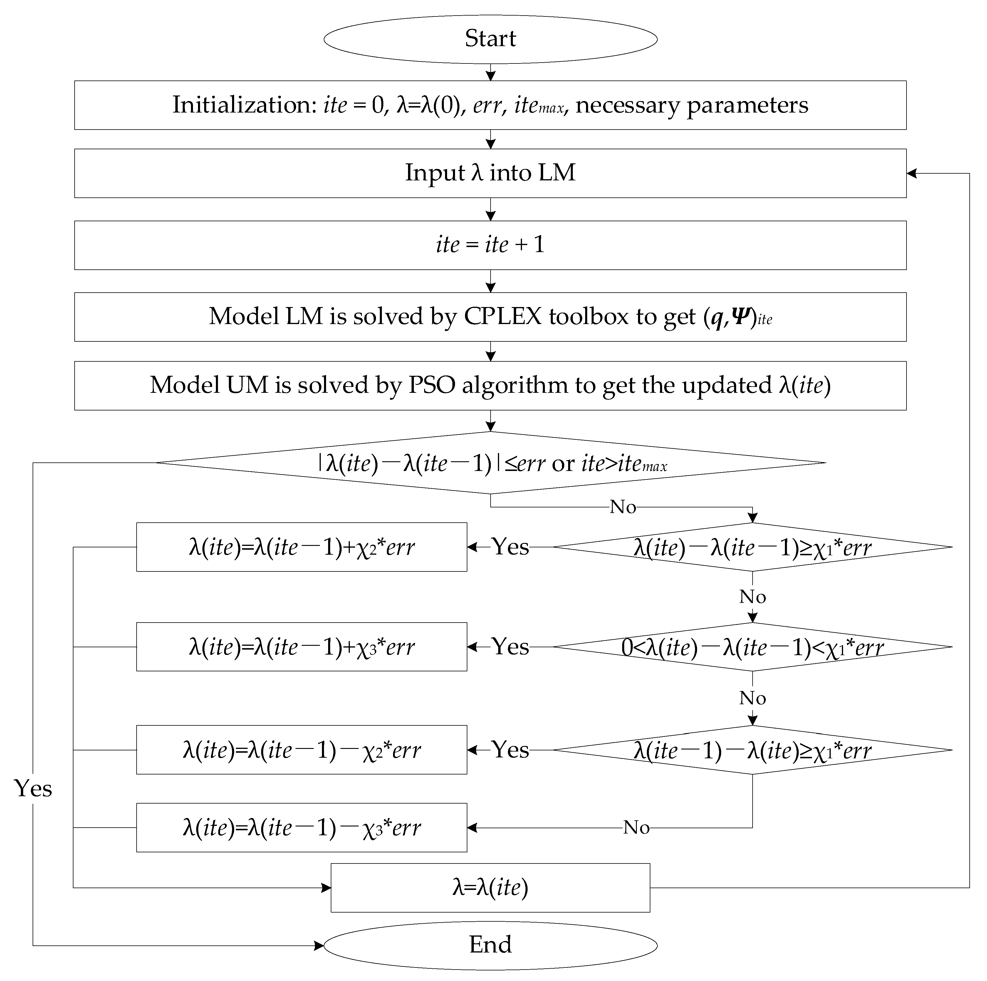
If the initial value is far from the optimal solution and the step size χ > 0 is small, the iteration will take a long time to approach the optimal solution. To address this, the convergence strategy is adjusted. Increase the step size to accelerate convergence when the current solution is far from the optimal solution. When the solution is close to the optimal value, set a smaller step size (not greater than err) to fine-tune and avoid overshooting the optimal solution. χ₁, χ_2, and χ₃ are custom-defined parameters, where χ₁ > χ₂ > 1 and χ₃ ∈ (0, 1). This adaptive adjustment of the step size enhances the efficiency and accuracy of the convergence process.

Adjusted convergence strategy for the CT algorithm:

(1)

If λ(ite) − λ(ite − 1) ≥ χ₁*err, then let λ(ite) = λ(ite − 1) + χ₂*err;

If 0 < λ(ite) − λ(ite − 1) < err, then let λ(ite) = λ(ite − 1) + χ₃*err.

(2)

If λ(ite − 1) − λ(ite) ≥ χ₁*err, then let λ(ite) = λ(ite − 1) − χ₂*err;

If 0 < λ(ite − 1) − λ(ite) < χ₁*err, then let λ(ite) = λ(ite − 1) − χ₃*err.

(3)

If |λ(ite) − λ(ite − 1)| ≤ err, the algorithm terminates and outputs the result λ(ite).

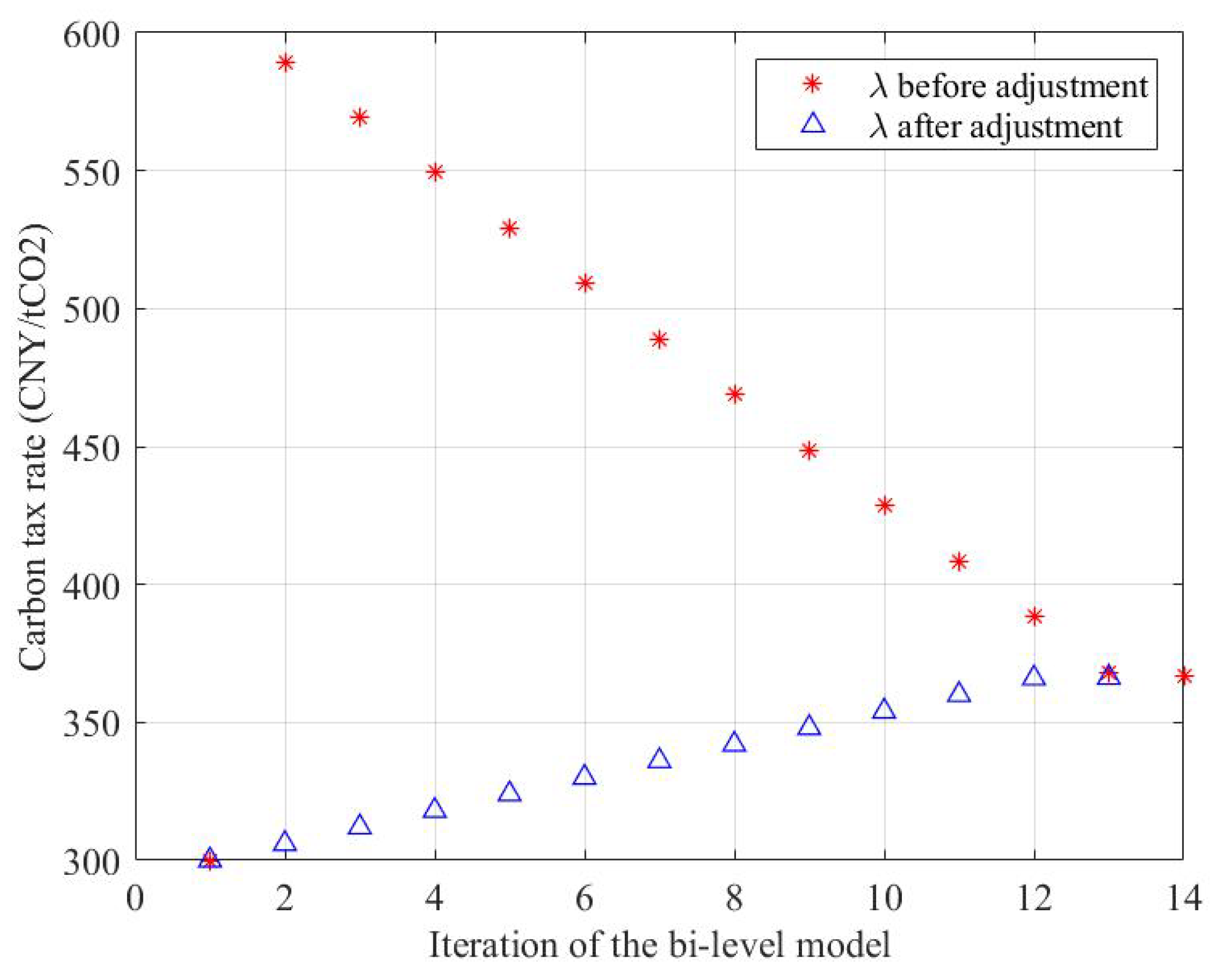
Figure 4 presents a schematic of the carbon tax rate gradually converging to the optimal solution during the iterative process.

Figure 5 shows a flowchart of the designed CT algorithm.

4. Numerical Experiments

4.1. The Input Data

Mitigating CO₂ emissions has garnered significant attention in China. This study selects the Beijing–Shanghai transportation corridor in China for a case analysis to validate the proposed methodology. This corridor encompasses five major cities: Beijing, Tianjin, Jinan, Nanjing, and Shanghai, as shown in Figure 6.

The freight rates for various freight modes are presented in

Table 3. Parameter values for utility function calculation.

Parameter		Value
		HSR	Road	Air
$p_{ij}^m$ (CNY/kg)	demand type n1	25	10	30
	demand type n2	10	5	15
$t_{wait}^m$ (h)	demand type n1	2	1	2
	demand type n2	12	9	12
$v^m$ (km/h)		250	65	-
$t_{door}^m$ (h)		4	1	5
$d^m$ (%)		1	2	0.5
$o^m$ (%)		95	75.5	76.7
${\sigma }^m$ (tCO2/kg-km)		1.19 × 10−8	4.79 × 10−8	5.64 × 10−7

. Demands with less stringent timeliness requirements permit extended waiting times at stations. The attribute values in the mode selection model are derived from Table 3 and

Table 4. Parameter values related to OD pairs.

OD	NO	${\mathit{l}}_{\mathit{i}\mathit{j}}^{\mathit{m}}$ (km)			${\mathit{t}}_{\mathit{w}\mathit{a}\mathit{y}}^{\mathit{i}\mathit{j},\mathit{a}\mathit{i}\mathit{r}}$ (h)	${\mathit{Q}}_{\mathit{i}\mathit{j},\mathit{n}}$ (ton)
		HSR	Road	Air		n1	n2
Beijing → Tianjin	OD1	137	137	-	-	145	752
Beijing → Jinan	OD2	406	410	-	-	43	225
Beijing → Nanjing	OD3	1023	1010	981	2.08	117	604
Beijing → Shanghai	OD4	1318	1209	1178	2.50	320	1654
Tianjin → Jinan	OD5	269	328	-	-	14	74
Tianjin → Nanjing	OD6	886	891	907	2.08	27	140
Tianjin → Shanghai	OD7	1181	1082	1133	2.08	72	371
Jinan → Nanjing	OD8	617	622	-	-	30	155
Jinan → Shanghai	OD9	912	829	852	1.58	86	448
Nanjing → Shanghai	OD10	295	307	-	-	235	1215

. The transportation network analyzed in this case study comprises 10 OD pairs, detailed in Table 4. Table 4 also provides the HSR, road, and air haul distances for each OD pair, along with the two types of freight demands. The emission factors set in this study are partly based on the literature [39,40]. These factors have inherent uncertainty owing to the varying assessment criteria and methodologies employed in their computation [41]. Freight rates can be obtained from publicly available information on transportation company websites. Freight demand is simulated using randomly generated values as actual data is often commercially sensitive and difficult to obtain.

The three freight modes exhibit distinct service ranges. The available freight modes for each OD pair are specified in

Table 5. Alternative freight modes for different OD pairs and demand types.

OD	Alternative Modes
	Demand Type n1	Demand Type n2
OD1	HSR, road	HSR, road
OD2	HSR, road	HSR, road
OD3	HSR, air	HSR, air
OD4	HSR, air	HSR, air
OD5	HSR, road	HSR, road
OD6	HSR, air	HSR, road, air
OD7	HSR, air	HSR, air
OD8	HSR, road	HSR, road
OD9	HSR, air	HSR, road, air
OD10	HSR, road	HSR, road

. Notably, air transportation does not operate on short-distance routes between certain OD pairs, while road transportation is unsuitable for long-distance express freight. Based on the speed and waiting time data in Table 3, road transportation can serve demand n₁ within 650 km and demand n₂ within 900 km.

The weights of each attribute, estimated via the maximum likelihood method, are as follows: $[{\alpha }_1,{\alpha }_2,{\alpha }_3,{\alpha }_4,{\alpha }_5]=$ [−0.041, −0.165, 0, 0, −1.2826]. During parameter estimation, reliability and safety were excluded due to their statistically insignificant contributions. The p-values for the remaining three attributes are below 0.15 (see

Table 6. Results of conditional maximum likelihood estimates.

Attributes	Estimate	Standard Error	Wald Chi-Square	Pr > ChiSq	Standardized Estimate
Economy	−0.041	0.0235	3.0485	0.0808	−0.1972
Timeliness	−0.165	0.1007	2.6848	0.1013	−0.497
Environmental negative externality	−1.2826	0.5916	4.7	0.0302	−0.1699

), indicating statistical significance.

Table 7. Loading capacities and operating costs of four HSR modes.

Parameter	Values of Different HSR Modes
	r1	r2	r3	r4
$c_{fix}^r$ (CNY)	5263	152.2	2346	18,770
$c_l^r$ (CNY/km)	-	-	18.6	148.9
$c_q^r$ (CNY/ton)	34.7	35.5	58.8	49.7
$N_r$ (ton)	27.6	2.4	12.6	120

outlines the loading capacities and operating costs of the four HSR modes. Cost data is based on the existing literature such as [30], yet in practice, cost estimation should be more systematic and comprehensive. The maximum service frequencies for the various HSR modes are presented in

Table 8. Maximum service frequencies of four HSR modes.

OD	HSR Mode r1	HSR Mode r2 and r3			HSR Mode r4
		${\mathit{\xi }}_{\mathit{i}\mathit{j},{\mathit{t}}_1}^{\mathit{p}\mathit{a}\mathit{s}}$	${\mathit{\xi }}_{\mathit{i}\mathit{j},{\mathit{t}}_2}^{\mathit{p}\mathit{a}\mathit{s}}$	${\mathit{\xi }}_{\mathit{i}\mathit{j},{\mathit{t}}_3}^{\mathit{p}\mathit{a}\mathit{s}}$	${\mathit{\xi }}_{\mathit{i}\mathit{j}}^{\mathit{f}\mathit{r}\mathit{e}}$
OD1	0	51	18	19	1
OD2	1	4	0	0	2
OD3	0	1	0	0	5
OD4	0	9	0	8	5
OD5	1	0	0	0	2
OD6	0	0	0	0	2
OD7	0	0	0	1	5
OD8	1	0	0	0	2
OD9	0	2	0	1	5
OD10	1	28	5	12	2

. The passenger train service frequencies used for HSR mode r_1- r₃ can be derived from the 12,306 China State Railway Group passenger ticket service system.

4.2. Results Analysis

In this section, the variable range of the carbon tax rate is set from 0 to 1000 CNY/tCO₂. The results of the following three scenarios are calculated.

Scenario #0: Set $\mathit{Q}={\mathit{Q}}_0$, $\lambda =0$.

Scenario #1: Set $\mathit{Q}=(1+3\%){\mathit{Q}}_0$, $\lambda =0$.

Scenario #2: Set $\mathit{Q}=(1+3\%){\mathit{Q}}_0$. The optimal $\lambda$ is obtained according to the methodology proposed.

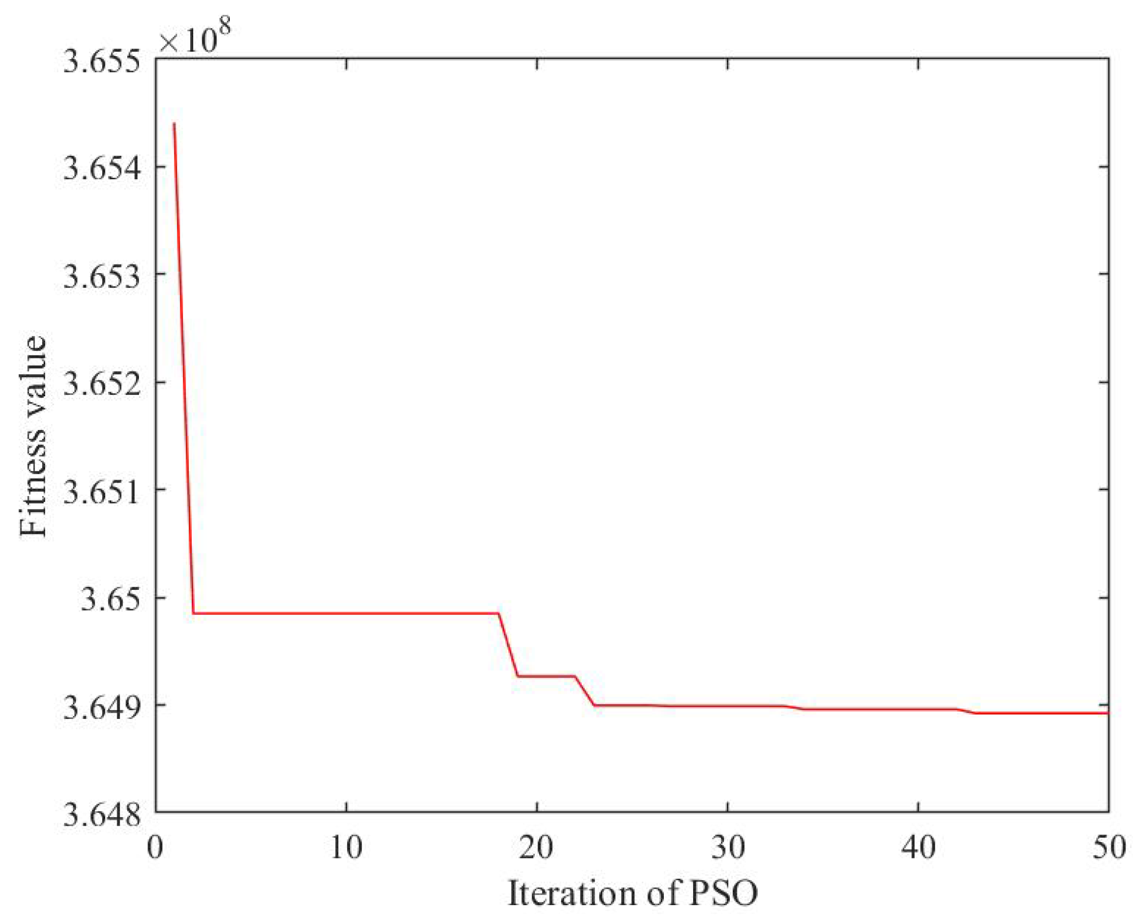
All experiments are coded in MATLAB R2018a and executed on a laptop with 1.80 GHz Intel Core and 8 GB of RAM. Figure 7 shows the convergence process of the PSO algorithm for solving the lower-level model in the last iteration between bi-levels. PSO parameter settings: c₁ = 1.5, c₂ = 1.5, 100 particles, 50 iterations. Figure 8 depicts the gradual convergence of carbon tax rate $\lambda$ to the optimal value during repeated iterations of the bi-level model, aligning with the algorithm design expectations outlined in Section 3.6.

The optimal carbon tax rate obtained in Scenario #2 is λ = 367.03 CNY/tCO₂. As shown in

Table 9. CO₂ emissions and HSR freight profits of Scenario #0–2.

Item	Scenario #0	Scenario #1	Scenario #2
optimal carbon tax rate (CNY/tCO2)	-	-	367.03
CO2 emissions (ton)	1131.914	1181.727	1131.913
Increase to Scenario #0	-	+4.40%	+0%
Increase to Scenario #1	-	-	−4.22%
HSR freight profits (CNY)	27,641,787.78	28,306,561.22	29,740,030.87
Increase to Scenario #0	-	+2.41%	+7.59%
Increase to Scenario #1	-	-	+5.06%
change in consumer surplus (CNY)	-	-	−11,628,746.67

, although transportation demand in Scenario #2 is higher than in Scenario #0, CO₂ emissions do not increase due to the carbon tax policy. In other words, an optimal policy is achieved.

According to Equation (33), Equation (42) can be derived to assess the impact of the carbon tax policy on consumer surplus. The superscripts pre and post refer to before and after the carbon tax policy application, respectively. It calculates the change in consumer surplus as the difference between consumer surplus under Scenario #2 (with the carbon tax policy) and Scenario #1 (without the carbon tax policy). The change in consumer surplus is found to be $\Delta CS$ = −11,628,746 CNY.

$$\Delta CS ={\displaystyle \sum _{ij\in \mathbb{O}\mathbb{D}}{\displaystyle \sum _{n\in \mathbb{N}}{Q}_{ij,n}\frac{1}{\left|{\alpha }_1\right|}\ln ({\displaystyle \sum _{m\in \mathbb{M}}\exp (V_{ij,n}^{post,m}}))}}-{\displaystyle \sum _{ij\in \mathbb{O}\mathbb{D}}{\displaystyle \sum _{n\in \mathbb{N}}{Q}_{ij,n}\frac{1}{\left|{\alpha }_1\right|}\ln ({\displaystyle \sum _{m\in \mathbb{M}}\exp (V_{ij,n}^{pre,m}}))}}$$

(42)

While the carbon tax policy reduces consumer surplus, the overall social welfare changes are complex, encompassing consumer surplus, producer surplus, government revenue, and environmental benefits. Table 9 shows that HSR freight profits increase by 5.06% post-carbon tax policy implementation. Producer surplus is measured by transportation profit. If non-green transportation modes have higher unit transportation profits than the green modes they are replaced by, modal shift may decrease producer surplus. However, the carbon tax policy promotes the reduction of transportation’s negative externalities and positively impacts emissions, air quality, and health. Government carbon tax revenue depends on levy system costs and potential tax revenue recycling, which are beyond this paper’s scope. This study focuses on reducing CO₂ emissions to a specific level while minimizing its impact on consumer surplus.

The mode split in Scenarios #0 and #1 is identical since neither incorporates the carbon tax policy. By comparing Scenarios #1 and #2, the changes in mode share before and after the implementation of the carbon tax policy can be observed. The total effect, as mentioned in

Table 10. Freight volumes of different modes in Scenario #1–2.

Freight Mode	Freight Volume (ton)		Increase to Scenario #1
	Scenario #1	Scenario #2
HSR	2536.924	2621.67	+3.34%
road	1927.163	1934.053	+0.36%
air	1825.093	1733.431	−5.02%

, indicates that the carbon tax policy in Scenario #2 has effectively encouraged a shift towards more environmentally friendly transportation modes.

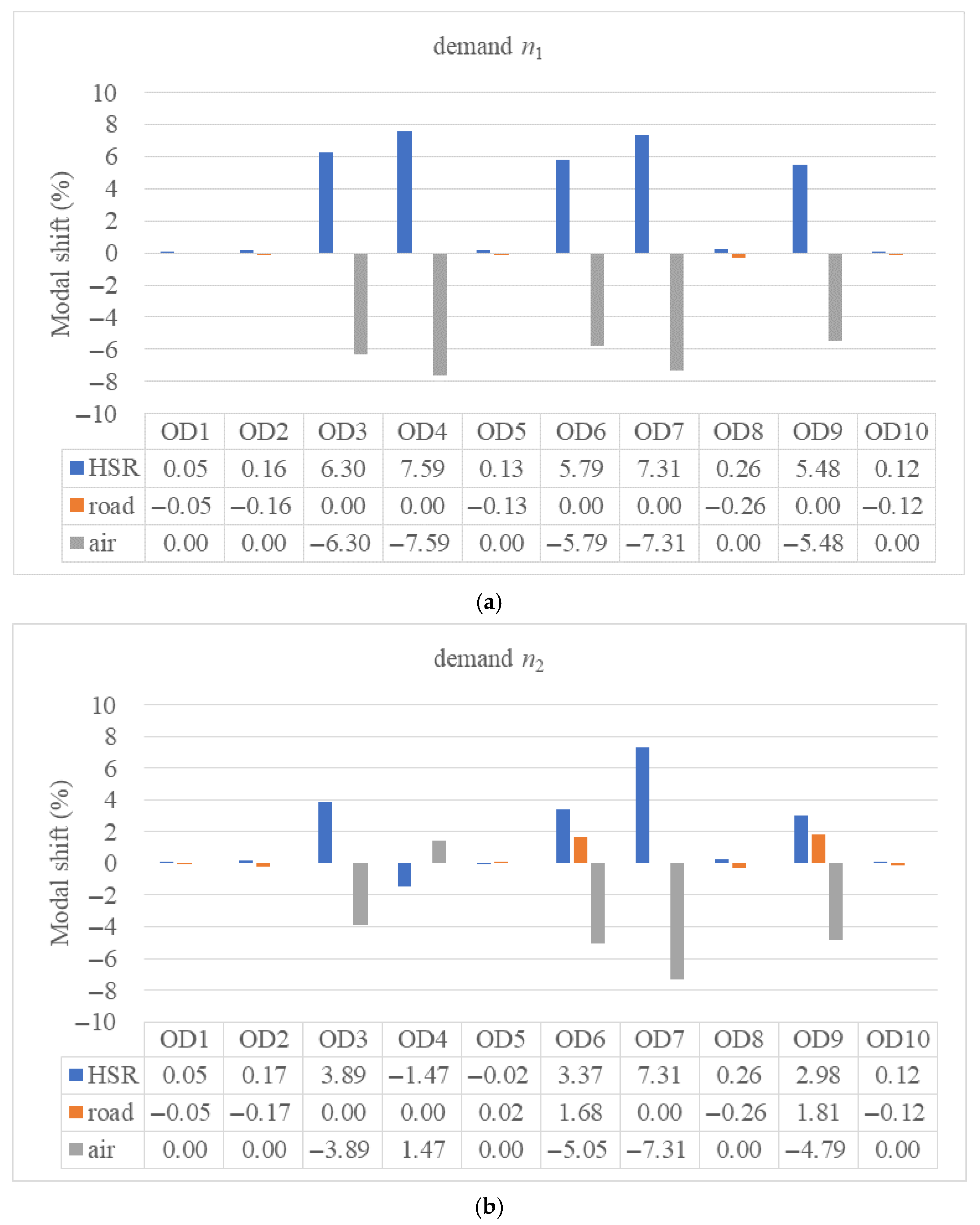
Figure 9 provides a detailed illustration of the modal shift for each OD pair and two types of freight demands. It is notable that the network comprises both sensitive and less sensitive segments. The carbon tax policy demonstrates a more pronounced effect in the medium- and long-distance transportation markets. This is attributed to the fact that HSR freight primarily competes with air transportation rather than road transportation in these markets. Air transportation is less environmentally friendly than road transportation. Furthermore, as the transportation distance increases, the carbon tax cost disparity between alternative modes widens, thereby accentuating the advantages of greener transportation options. An exception is observed for demand n₂ of OD4, where the limited capacity of HSR freight restricts its ability to fully accommodate the demand attracted.

The detailed allocation of HSR freight volumes across different patterns and the required service frequencies are presented in

Table 11. Required service frequency for each HSR mode.

OD	HSR Mode r1	HSR Mode r2			HSR Mode r3			HSR Mode r4
		Trains in t1	Trains in t2	Trains in t3	Trains in t1	Trains in t2	Trains in t3
OD1	0	47	16	14	2	2	0	0
OD2	0	0	0	0	0	0	0	1
OD3	0	0	0	0	1	0	0	3
OD4	0	0	0	0	9	0	8	5
OD5	1	0	0	0	0	0	0	0
OD6	0	0	0	0	0	0	0	1
OD7	0	0	0	0	0	0	0	2
OD8	0	0	0	0	0	0	0	1
OD9	0	0	0	0	0	0	0	2
OD10	1	23	0	12	5	5	0	2

and

Table 12. Freight volume assignment for each mode of HSR (ton).

Demand Type	OD	HSR Mode r1	HSR Mode r2			HSR Mode r3			HSR Mode r4
			Trains in t1	Trains in t2	Trains in t3	Trains in t1	Trains in t2	Trains in t3
n1	OD1	0	0	2.28	33.60	0	0	0	0
	OD2	0	0	0	0	0	0	0	15.21
	OD3	0	0	0	0	0	0	0	62.51
	OD4	0	0	0	0	0	0	100.80	64.71
	OD5	4.34	0	0	0	0	0	0	0
	OD6	0	0	0	0	0	0	0	14.58
	OD7	0	0	0	0	0	0	0	37.26
	OD8	0	0	0	0	0	0	0	13.26
	OD9	0	0	0	0	0	0	0	45.15
	OD10	27.60	0	0	28.80	0	0	0	17.12
n2	OD1	0	112.80	36.12	0	24.16	25.20	0	0
	OD2	0	0	0	0	0	0	0	83.56
	OD3	0	0	0	0	12.60	0	0	297.49
	OD4	0	0	0	0	113.40	0	0	535.29
	OD5	23.26	0	0	0	0	0	0	0
	OD6	0	0	0	0	0	0	0	56.79
	OD7	0	0	0	0	0	0	0	193.19
	OD8	0	0	0	0	0	0	0	71.640
	OD9	0	0	0	0	0	0	0	167.37
	OD10	0	55.20	0	0	60.52	63.00	0	222.88

. It is evident that the required service frequency for HSR freight services for OD4 reaches the maximum value specified in Table 7, with each train’s capacity being fully utilized.

4.3. Sensitivity Analysis

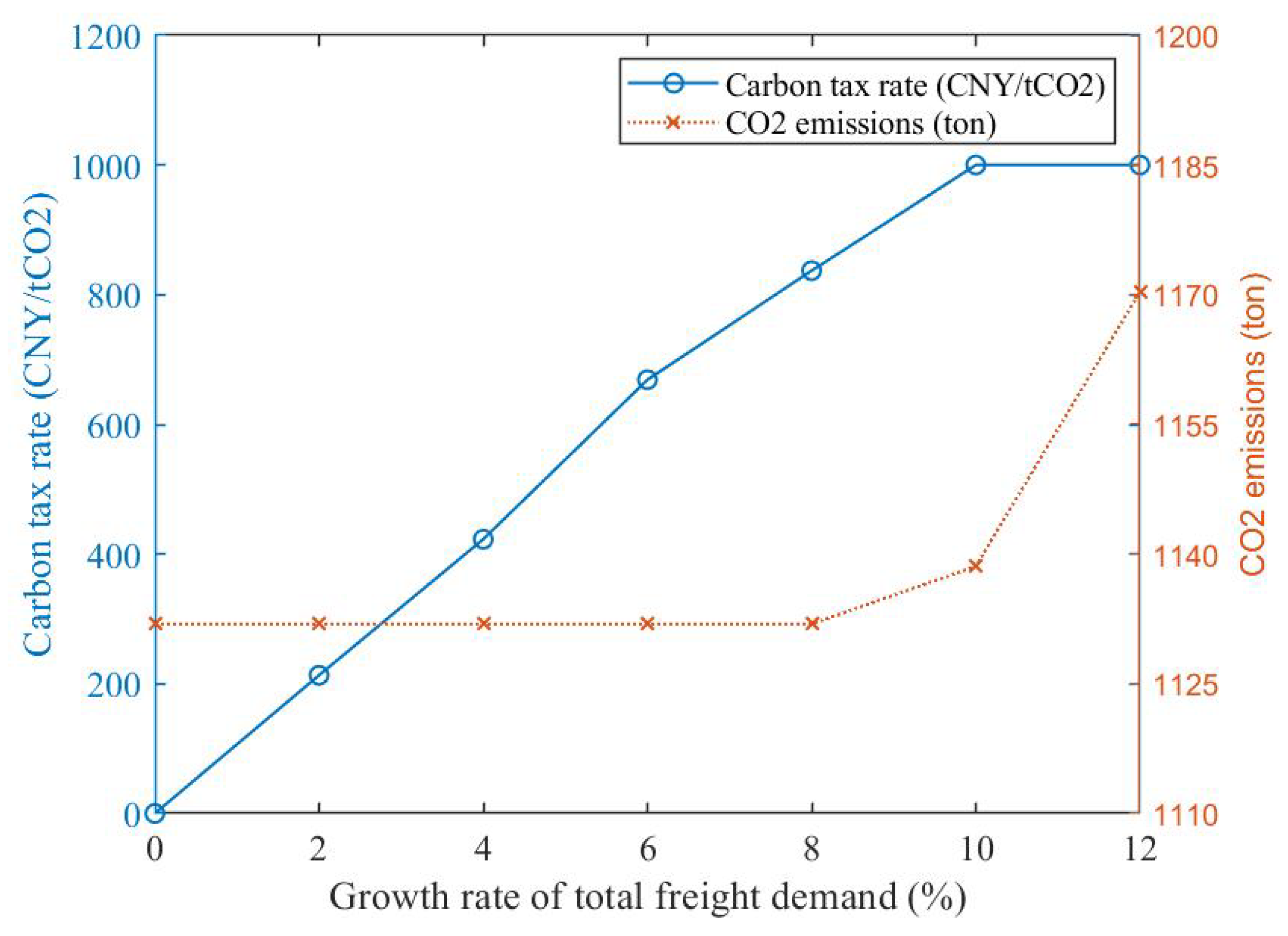
In Section 4.2, a 3% growth rate for freight demand is assumed. The following discussion explores the CO₂ emission outcomes and carbon tax rate formulations under varying demand growth rates, specifically at values of 2%, 4%, 6%, 8%, 10%, and 12%. The computational results are presented in Figure 10. It is evident that as demand increases, it becomes progressively more challenging to reduce CO₂ emissions to the baseline level (the level under the initial freight demand), and the carbon tax rate gradually approaches its maximum limit.

Achieving the government’s complete decarbonization objective necessitates reducing unnecessary freight demand. However, the growth in freight activities is closely tied to economic growth and hard to decouple. One potential strategy to reduce freight demand involves restructuring supply chain management, such as promoting localized production to reduce the transportation distance of materials and products.

Figure 10 indicates that as freight demand increases, CO₂ emissions cannot be reduced to the initial level, and the optimal carbon tax rate rises to the set cap of 1000 CNY/tCO₂. If this carbon tax ceiling is disregarded, would there perpetually exist an appropriate rate to revert CO₂ emissions to the initial level? Subsequent analysis addresses this question.

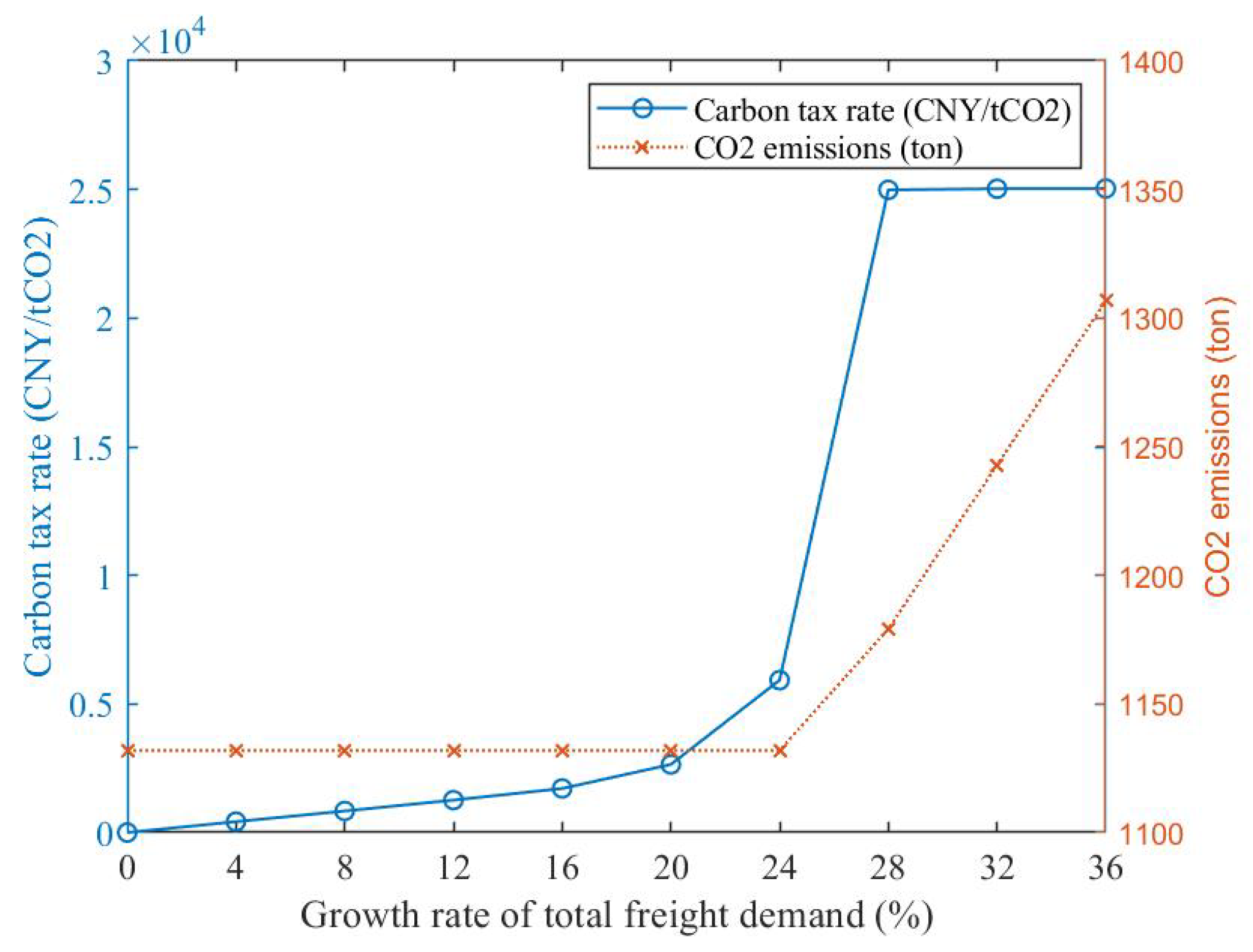
An extremely high value is assigned to the carbon tax rate cap during model solving to negate its influence. Experiment results for demand growth rates of 12%, 16%, 20%, 24%, 28%, and 32% are depicted in Figure 11. Results for demand growth rates of 0%, 4%, and 8% are derived from Figure 10, as their optimal carbon tax rates do not exceed the previously set upper limit of 1000 CNY/tCO₂. Consequently, removing the cap does not affect these results. In Figure 10, after the demand growth rate reaches 10%, CO₂ emissions cannot be reduced to the initial level. Once the carbon tax rate upper limit is eliminated, full decarbonization for demand growth rates of 12%, 16%, 20%, and 24% can be achieved by setting optimal carbon tax rates at 1260.53, 1712.83, 2646.02, and 5923.62 CNY/tCO₂, respectively. However, an unrestricted carbon tax is not always practical for decarbonization. As shown in Figure 11, after the demand growth rate reaches 28%, the increased CO₂ emissions due to freight demand growth cannot be entirely eliminated. Moreover, as demand increases, the optimal carbon tax rate does not rise indefinitely but gradually approaches a stable value. This indicates that even if a carbon tax higher than this stable value is set, CO₂ emissions cannot be reduced further. As freight transportation demand increases, the maximum modal shift achievable through carbon taxes cannot reduce CO₂ emissions to the original level.

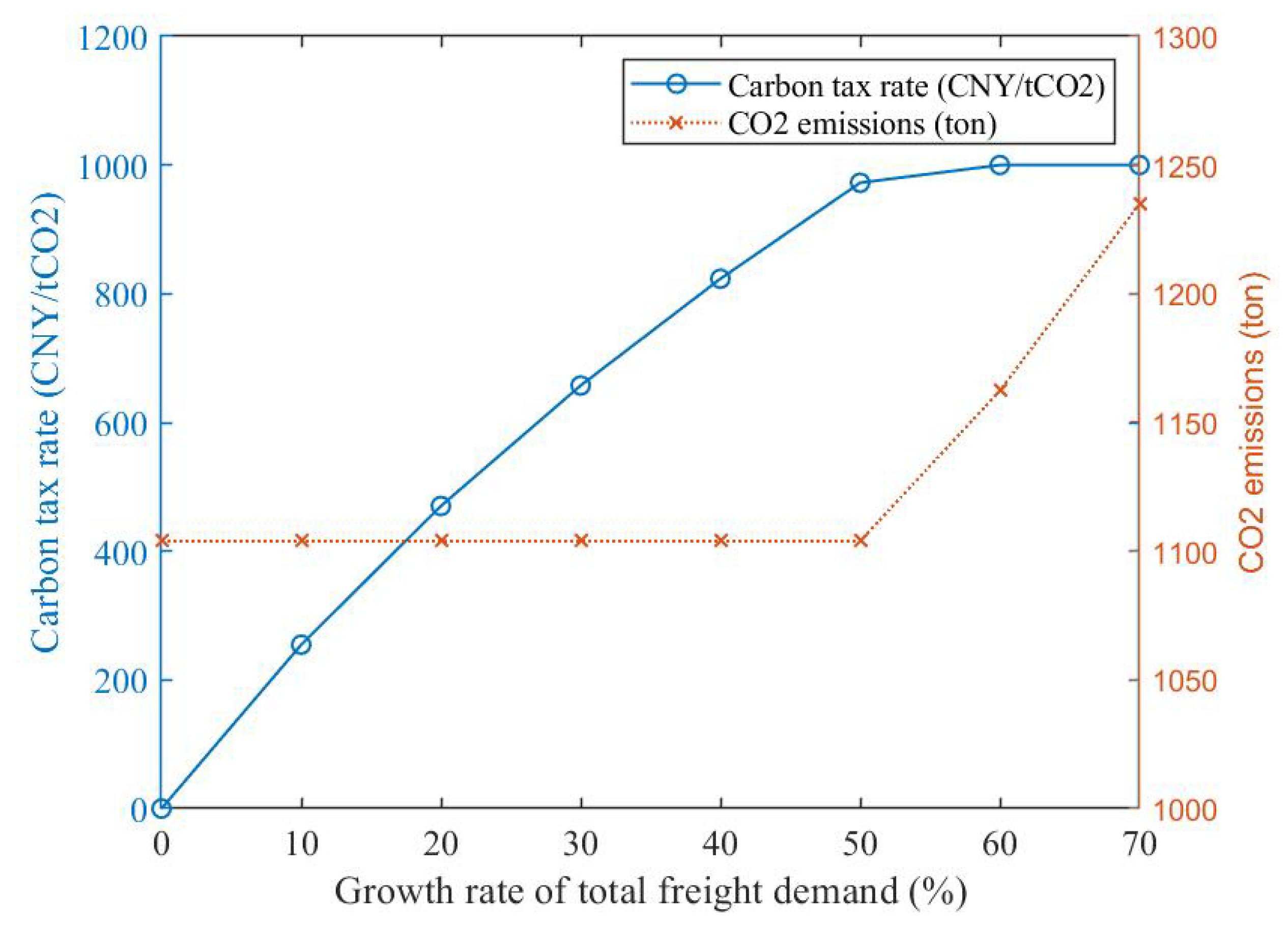
The limited modal shift achievable through the carbon tax policy may be associated with the freight capacity of HSR. Assuming the actual freight volume of HSR is equivalent to its freight demand, i.e., HSR capacity limitations are disregarded, then the results presented in Figure 12 are obtained under demand growth rates of 10%, 20%, 30%, 40%, 50%, 60%, and 70%. It is evident that even with substantial demand increases, the transportation system can achieve decarbonization at a lower carbon tax rate, provided HSR transportation capacity constraints are not considered. A prerequisite for effectively utilizing modal shift as a tool is adequate green transportation infrastructure within the freight corridor. Otherwise, insufficient transportation supply may prevent some shippers from using green transportation modes, even if they are willing to do so.

5. Discussion

5.1. Management Insights

Drawing from the study’s findings, the following management insights are proposed to guide stakeholders in achieving sustainable development:

(1) Implement and dynamically adjust carbon tax policies

Carbon tax policies can effectively incentivize modal shifts toward environmentally friendly transportation modes such as HSR. However, the efficacy of these policies hinges on continuous monitoring and dynamic adjustment of tax rates. Policymakers should adopt a data-driven approach to calibrate tax rates, balancing emission reduction targets with economic impacts. For instance, the case study shows that a carbon tax of 367.03 CNY/tCO₂ can offset the additional CO₂ emissions resulting from a 3% increase in freight demand. This underscores the importance of adaptive policy-making to ensure the sustained effectiveness of carbon tax policies as market conditions evolve. The successful implementation of carbon tax policies depends on several critical factors. First, the capacity of HSR infrastructure must be sufficient to accommodate the potential increase in freight demand resulting from modal shift. Second, policymakers should consider the regional differences in freight transportation demand and HSR service availability when designing and implementing carbon tax policies. The case study reveals that the sensitivity of the freight market to carbon tax policies varies across different OD pairs and freight demand types. For example, medium- and long-distance transport markets are more responsive to carbon tax policies due to the competition between HSR and air transport.

(2) Invest in green transportation infrastructure

Adequate green transportation infrastructure, particularly HSR capacity, is essential to support modal shifts and achieve decarbonization goals. The study reveals that HSR infrastructure constraints can significantly limit the emission reduction potential of carbon tax policies. Therefore, investing in the expansion and enhancement of HSR infrastructure to ensure sufficient capacity and coverage—especially in regions with high modal shift potential—is critical. This enables stakeholders to adopt environmentally friendly transportation options and ensures the long-term sustainability of the express freight sector. Without adequate capacity, even the most favorable policies may fail to induce the desired modal shift. Hence, it is crucial to prioritize infrastructure development in regions where the potential for modal shift is high. This encompasses not only building more tracks and stations but also improving related logistics facilities and services to make HSR freight operations efficient and attractive.

Tailoring policies to local contexts can maximize emission reduction outcomes. For example, areas with underdeveloped railway infrastructure may have limited capacity to shift freight from road and air to HSR. In such regions, policies should focus on gradually building up rail capacity while simultaneously encouraging shipping companies to opt for more environmentally friendly transport modes. Additionally, promoting localized production and optimizing supply chain structures can reduce transportation distances and associated emissions. This can be achieved by offering incentives for businesses to establish production facilities closer to their target markets, thereby reducing reliance on long-haul transportation.

(3) Encourage comprehensive decarbonization strategies

The MNL model employed in this study demonstrates that shippers’ mode choices are influenced by multiple factors beyond cost, including timeliness. While economic incentives like carbon taxes are crucial, they must be complemented with improvements in the service quality of greener transport modes. For example, enhancing the timeliness of HSR freight services can make them more attractive to shippers. Furthermore, a comprehensive approach should evaluate the potential for modal shift across different regions and transportation corridors. This involves identifying which routes are most likely to achieve significant emission reductions through modal shift and prioritizing policy interventions and infrastructure investments in these areas.

(4) Strengthen stakeholder collaboration

The bi-level optimization model highlights the interdependencies among policymakers, HSR operators, and shippers. Effective decarbonization demands collaboration across these stakeholders. For instance, HSR operators can work with policymakers to synchronize service enhancements with modal shift incentives. This coordinated strategy ensures policies and operations are mutually reinforcing, fostering sustainable outcomes in the express freight sector.

5.2. Limitations

This study offers useful insights into China’s express freight sector decarbonization via modal shifts and carbon tax policies, but several limitations should be noted.

(1) Model assumptions: The bi-level model simplifies reality by focusing on cost and service factors for shipper mode choices and government objectives of consumer surplus and emissions reduction. It assumes flexible HSR freight capacity allocation, but practical constraints like train pathing and passenger service schedules may limit this flexibility. However, with the ongoing development of HSR freight services, the potential for separating passenger and freight services is becoming increasingly feasible.

(2) Data limitations: The case analysis is based on data from the Beijing–Shanghai corridor and uses industry estimates for some parameters due to the lack of precise market data, which introduces uncertainty.

(3) Stakeholder scope: The analysis centers on policymakers, HSR operators, and shippers, but other stakeholders such as road and air transport companies, and logistics service providers also play significant roles. Their responses to carbon tax policies could influence modal shift dynamics and emission reduction effectiveness.

(4) Dynamic and long-term effects: The study employs a static framework to analyze carbon tax policies. Long-term factors such as technological advancements and infrastructure development may affect the sustainability of modal shifts and emission reductions.

(5) Policy integration: The study primarily focuses on carbon tax policies and does not fully explore interactions with other policy instruments like subsidies and regulations. Future research could investigate integrated policy packages to enhance decarbonization strategies.

5.3. Future Research

Future research could extend this work in the following meaningful directions:

(1) Countrywide network expansion: Future research could expand the study to a countrywide network. This would involve collecting and integrating data from multiple corridors and regions across China, considering variations in economic conditions, infrastructure development, and policy implementations. A countrywide analysis would offer a more comprehensive understanding of how carbon tax policies and HSR services can be optimized within different regional contexts and help identify regions with the highest potential for modal shift and emission reductions.

(2) Dynamic modeling: Incorporating a dynamic component into the model is another valuable avenue for future research. This could involve considering short-term and long-term variations in freight demand, as well as the evolving nature of transportation technologies and energy sources. For example, the model could account for advancements in battery technology for electric vehicles, improvements in aircraft fuel efficiency, or the development of sustainable aviation fuels. These technological advancements could alter the cost structures and environmental performances of different transportation modes over time. A dynamic model could also allow for the simulation of policy adjustments in response to changing market conditions and environmental targets.

(3) Integrated revenue management strategies: Future research could investigate the potential for integrating revenue management strategies into HSR freight operations. Strategies such as dynamic pricing and inventory control could enhance the market competitiveness of HSR freight and improve its profitability. This could involve developing models that optimize pricing structures based on demand fluctuations, capacity constraints, and competition from other transportation modes. It could also explore how revenue from carbon taxes could be recycled to support the development of green transportation infrastructure and technologies.

(4) Enhanced data collection: Future research could enhance data collection methods to obtain more comprehensive and precise input parameters. This includes detailed cost breakdowns from transportation operators and actual freight demand data to improve model accuracy. Additionally, advanced techniques such as machine learning could be employed to obtain more accurate demand prediction data.

(5) Autonomous train-control integration: Future research could integrate Autonomous Train Control Systems (ATCS) [42] into HSR freight planning. By incorporating train-centric communication, moving-block signaling, and real-time slot reallocation, HSR freight capacity becomes a dynamic parameter driven by ATCS rather than a fixed value. This integration would enable instantaneous adjustments to freight capacity in response to demand fluctuations, reducing the risk of capacity shortages that could hinder modal shifts to HSR. Additionally, AI-optimized timetables dynamically balance passenger and freight priorities, reallocating excess passenger slots to freight in real-time. This would strengthen the alignment of HSR capacity with fluctuating demand, prevent congestion, accelerate freight delivery, and enhance the reliability and timeliness of HSR freight services. Ultimately, this would drive modal shift and reduce CO₂ emissions more effectively.

6. Conclusions

This study addresses the pressing issue of decarbonizing the express freight market, which is facing a surge in demand. By implementing an optimized carbon tax policy, shippers are incentivized to select greener freight modes. This problem is formulated as a bi-level model that integrates cargo flow assignment, transportation mode choice, and carbon tax design. A hybrid algorithm combining PSO and CPLEX is developed to solve this model. The case study in China’s Beijing–Shanghai corridor demonstrates the methodology’s effectiveness.

The initial CO₂ emissions from the transport system in the case study network amount to 1131.914 tons. If transportation demand grows by 3% without any policy measures being implemented, the emissions under the current modal split will increase to 1181.727 tons. To effectively curb the additional CO₂ emissions resulting from the demand growth, the study recommends imposing a carbon tax of 367.03 CNY/tCO₂. Compared with the pre-carbon tax situation, the carbon tax policy induces the following modal shifts: HSR freight increases by 3.34%, road freight rises by 0.36%, and air freight decreases by 5.02%. The analysis reveals that the medium/long-distance transport market is more sensitive to carbon tax policies, which leads to more pronounced modal shifts.

Sensitivity analysis experiments under varying demand growth rates reveal that achieving a return to initial emission levels via carbon tax policy-induced modal shifts is not guaranteed. On the one hand, as freight demand increases, the required carbon tax approaches its upper limit. On the other hand, HSR, as a relatively nascent freight transportation mode, currently faces capacity constraints that prevent it from fully accommodating the demand of potential users. Even if the carbon tax cap is removed, it may still be insufficient to fully offset the CO₂ emissions resulting from growing transportation demand. Therefore, adequate green transportation infrastructure is essential for decarbonizing China’s express freight market. Moreover, measures to avoid unnecessary transportation can be implemented in tandem to enhance the effectiveness of emission reduction strategies.

This study provides insights into China’s express freight sector decarbonization through modal shifts and carbon tax policies, but has limitations in model assumptions, data scope, stakeholder coverage, dynamic effects, and policy integration. Future research could expand to a countrywide network, incorporate dynamic modeling, explore integrated revenue management strategies, enhance data collection methods for more accurate demand predictions, and integrate ATCS into HSR freight planning.

References

1. Kaack, L.H.; Vaishnav, P.; Morgan, M.G.; Azevedo, I.L.; Rai, S. Decarbonizing intraregional freight systems with a focus on modal shift. Environ. Res. Lett. 2018, 13, 083001. [Google Scholar] [CrossRef]
2. Tattini, J.; Gargiulo, M.; Karlsson, K. Reaching carbon neutral transport sector in Denmark—Evidence from the incorporation of modal shift into the TIMES energy system modeling framework. Energy Policy 2018, 113, 571–583. [Google Scholar] [CrossRef]
3. NBS National Data. Available online: https://data.stats.gov.cn/easyquery.htm?cn=C01 (accessed on 1 May 2025).
4. Zhao, C.; Zhou, B. Impact of Express Delivery Industry’s Development on Transportation Sector’s Carbon Emissions: An Empirical Analysis from China. Sustainability 2021, 13, 8908. [Google Scholar] [CrossRef]
5. Bi, M.; He, S.; Xu, W. Express delivery with high-speed railway: Definitely feasible or just a publicity stunt. Transp. Res. Part A-Policy Pract. 2019, 120, 165–187. [Google Scholar] [CrossRef]
6. To, W.M. Greenhouse gases emissions from the logistics sector: The case of Hong Kong, China. J. Clean. Prod. 2015, 103, 658–664. [Google Scholar] [CrossRef]
7. Masone, A.; Marzano, V.; Simonelli, F.; Sterle, C. Exact and heuristic approaches for the Modal Shift Incentive Problem. Socio-Econ. Plan. Sci. 2024, 93, 101874. [Google Scholar] [CrossRef]
8. Paladugula, A.L.; Kholod, N.; Chaturvedi, V.; Ghosh, P.P.; Pal, S.; Clarke, L.; Evans, M.; Kyle, P.; Koti, P.N.; Parikh, K.; et al. A multi-model assessment of energy and emissions for India’s transportation sector through 2050. Energy Policy 2018, 116, 10–18. [Google Scholar] [CrossRef]
9. Liu, P.; Mu, D.; Gong, D. Eliminating overload trucking via a modal shift to achieve intercity freight sustainability: A system dynamics approach. Sustainability 2017, 9, 398. [Google Scholar] [CrossRef]
10. Zhou, Y.; Fang, W.; Li, M.; Liu, W. Exploring the impacts of a low-carbon policy instrument: A case of carbon tax on transportation in China. Resour. Conserv. Recycl. 2018, 139, 307–314. [Google Scholar] [CrossRef]
11. Qiu, R.; Xu, J.; Xie, H.; Zeng, Z.; Lv, C. Carbon tax incentive policy towards air passenger transport carbon emissions reduction. Transport. Res. Part D-Transport. Environ. 2020, 85, 102441. [Google Scholar] [CrossRef]
12. Wang, M.; Liu, K.; Choi, T.-M.; Yue, X. Effects of Carbon Emission Taxes on Transportation Mode Selections and Social Welfare. IEEE Trans. Syst. Man Cybern.-Syst. 2015, 45, 1413–1423. [Google Scholar] [CrossRef]
13. Bouchery, Y.; Ghaffari, A.; Jemai, Z.; Fransoo, J. Sustainable transportation and order quantity: Insights from multiobjective optimization. Flex. Serv. Manuf. J. 2016, 28, 367–396. [Google Scholar] [CrossRef]
14. Tao, X.; Wu, Q.; Zhu, L. Mitigation potential of CO2 emissions from modal shift induced by subsidy in hinterland container transport. Energy Policy 2017, 101, 265–273. [Google Scholar] [CrossRef]
15. Choi, B.; Park, S.-i.; Lee, K.-D. A System Dynamics Model of the Modal Shift from Road to Rail: Containerization and Imposition of Taxes. J. Adv. Transp. 2019, 2019, 7232710. [Google Scholar] [CrossRef]
16. Kundu, T.; Sheu, J.-B. Analyzing the effect of government subsidy on shippers’ mode switching behavior in the Belt and Road strategic context. Transp. Res. Part E-Logist. Transp. Rev. 2019, 129, 175–202. [Google Scholar] [CrossRef]
17. Chen, K.; Xin, X.; Niu, X.; Zeng, Q. Coastal transportation system joint taxation-subsidy emission reduction policy optimization problem. J. Clean. Prod. 2020, 247, 119096. [Google Scholar] [CrossRef]
18. Guo, T.; Liu, P.; Wang, C.; Xie, J.; Du, J.; Lim, M.K. Toward sustainable port-hinterland transportation: A holistic approach to design modal shift policy mixes. Transp. Res. Part A-Policy Pract. 2023, 174, 103746. [Google Scholar] [CrossRef]
19. Nassar, R.F.; Ghisolfi, V.; Annema, J.A.; van Binsbergen, A.; Tavasszy, L.A. A system dynamics model for analyzing modal shift policies towards decarbonization in freight transportation. Res. Transp. Bus. Manag. 2023, 48, 100966. [Google Scholar] [CrossRef]
20. Takman, J.; Gonzalez-Aregall, M. Public policy instruments to promote freight modal shift in Europe: Evidence from evaluations. Transp. Rev. 2024, 44, 612–633. [Google Scholar] [CrossRef]
21. Shen, J.Q.; Liu, H.; Zhang, R. Railway pricing for automobile transport based on discrete choice model and cost accounting. Res. Transp. Bus. Manag. 2025, 59, 101295. [Google Scholar] [CrossRef]
22. Hoffrichter, A.; Silmon, J.; Iwnicki, S.; Hillmansen, S.; Roberts, C. Rail freight in 2035-traction energy analysis for high-performance freight trains. Proc. Inst. Mech. Eng. Part F J. Rail Rapid Transit 2012, 226, 568–574. [Google Scholar] [CrossRef]
23. Jia, X.; He, R.; Chai, H. Optimizing the Number of Express Freight Trains on a High-speed Railway Corridor by the Departure Period. IEEE Access 2020, 8, 100058–100072. [Google Scholar] [CrossRef]
24. Yu, X.; Lang, M.; Gao, Y.; Wang, K.; Su, C.-H.; Tsai, S.-B.; Huo, M.; Yu, X.; Li, S. An Empirical Study on the Design of China High-Speed Rail Express Train Operation Plan-From a Sustainable Transport Perspective. Sustainability 2018, 10, 2478. [Google Scholar] [CrossRef]
25. Yu, X.; Lang, M.; Zhang, W.; Li, S.; Zhang, M.; Yu, X. An Empirical Study on the Comprehensive Optimization Method of a Train Diagram of the China High Speed Railway Express. Sustainability 2019, 11, 2141. [Google Scholar] [CrossRef]
26. Li, S.; Zhu, M.; Zuo, D.; Guo, C.; Shi, L. A robust optimisation approach of train timetabling for freight transportation using high-speed railway. Transp. A-Transp. Sci. 2024, 2385874. [Google Scholar] [CrossRef]
27. Li, S.; Zuo, D.; Li, W.; Zhang, Y.; Shi, L. Freight train line planning for large-scale high-speed rail network: An integer Benders decomposition-based branch-and-cut algorithm. Transp. Res. Part E-Logist. Transp. Rev. 2024, 192, 103750. [Google Scholar] [CrossRef]
28. Wang, X.; Zhen, L.; Wang, S. Optimizing an express delivery mode based on high-speed railway and crowd-couriers. Transp. Policy 2024, 159, 157–177. [Google Scholar] [CrossRef]
29. Zhang, D.; Zhou, F.-R.; Ao, W.K.; Guo, Z.-H.; Chen, Z.-W. Optimization of cargo distribution for high-speed freight trains to overcome strong wind conditions. Eng. Appl. Comput. Fluid Mech. 2024, 18, 2434008. [Google Scholar] [CrossRef]
30. Li, S.; Chen, X.; Lang, M. A hybrid heuristic algorithm for high-speed rail line planning problem with multiple transport organization modes. Res. Transp. Bus. Manag. 2025, 60, 101328. [Google Scholar] [CrossRef]
31. Liang, X.-H.; Tan, K.-H. Market potential and approaches of parcels and mail by high speed rail in China. Case Stud. Transp. Policy 2019, 7, 583–597. [Google Scholar] [CrossRef]
32. Small, K.A.; Rosen, H.S. Applied welfare economics with discrete choice models. Econom. J. Econom. Soc. 1981, 49, 105–130. [Google Scholar] [CrossRef]
33. Yang, H.; Ma, W.; Wang, Q.; Wang, K.; Zhang, Y. Welfare implications for air passengers in China in the era of high-speed rail. Transp. Policy 2020, 95, A1–A13. [Google Scholar] [CrossRef]
34. Vaze, V.; Luo, T.; Harder, R. Impacts of airline mergers on passenger welfare. Transp. Res. Part E Logist. Transp. Rev. 2017, 101, 130–154. [Google Scholar] [CrossRef]
35. IPCC. Global Warming of 1.5 °C; IPCC: Geneva, Switzerland, 2015. [Google Scholar]
36. Benayed, O.; Blair, C.E. Computational Difficulties of Bilevel Linear Programming. Oper. Res. 1990, 38, 556–560. [Google Scholar] [CrossRef]
37. Bard, J.F. Some properties of the bilevel programming problem. J. Optim. Theory Appl. 1991, 68, 371–378. [Google Scholar] [CrossRef]
38. Kennedy, J.; Eberhart, R. Particle swarm optimization. In Proceedings of the Proceedings of ICNN’95-International Conference on Neural Networks, Perth, WA, Australia, 27 November–1 December 1995; pp. 1942–1948. [Google Scholar]
39. Chao, C.-C. Assessment of carbon emission costs for air cargo transportation. Transport. Res. Part D-Transport. Environ. 2014, 33, 186–195. [Google Scholar] [CrossRef]
40. Lin, B.L.; Liu, C.; Wang, H.J.; Lin, R.X. Modeling the railway network design problem: A novel approach to considering carbon emissions reduction. Transport. Res. Part D-Transport. Environ. 2017, 56, 95–109. [Google Scholar] [CrossRef]
41. Van Fan, Y.; Perry, S.; Klemes, J.J.; Lee, C.T. A review on air emissions assessment: Transportation. J. Clean. Prod. 2018, 194, 673–684. [Google Scholar] [CrossRef]
42. Song, H.; Gao, S.; Li, Y.; Liu, L.; Dong, H. Train-Centric Communication Based Autonomous Train Control System. IEEE Trans. Intell. Veh. 2023, 8, 721–731. [Google Scholar] [CrossRef]
Figure 1. Model framework.
Symmetry 17 01364 g001
Figure 2. Categorization of HSR passenger trains based on departure and arrival times.
Symmetry 17 01364 g002
Figure 3. Decarbonization process via carbon taxation and modal shift.
Symmetry 17 01364 g003
Figure 4. Convergence process diagram of the proposed bi-level model.
Symmetry 17 01364 g004
Figure 5. Flowchart of the CT algorithm.
Symmetry 17 01364 g005
Figure 6. Beijing–Shanghai freight transportation line in China.
Symmetry 17 01364 g006
Figure 7. Convergence trend of the lower-level model solution.
Symmetry 17 01364 g007
Figure 8. Convergence trend of the bi-level model solution.
Symmetry 17 01364 g008
Figure 9. Changes in mode split before and after carbon tax policy implementation. (a) shows the modal shift for each OD with demand n1. (b) shows the modal shift for each OD with demand n2.
Symmetry 17 01364 g009
Figure 10. Changes in carbon tax rates and CO2 emissions with increasing demand.
Symmetry 17 01364 g010
Figure 11. Changes in carbon tax rates and CO2 emissions with increasing demand (without carbon tax cap limitation).
Symmetry 17 01364 g011
Figure 12. Changes in carbon tax rates and CO2 emissions with increasing demand (without HSR freight capacity limitations).
Symmetry 17 01364 g012