Research on Intelligent Production Optimization of Low-Permeability Tight Gas Wells

Abstract

Gas well production prediction is an important means to determine the economic benefits of gas field development, and it is the key to realize the optimization of gas well production. However, with the continuous development of gas fields, the increasing number of low-yield and low-efficiency wells disrupted the original symmetry in the overall well distribution and production structure. Traditional production capacity prediction methods are difficult to adapt to complex geological conditions and dynamic production characteristics and cannot meet the requirements of refined management of gas fields. In this paper, a CNN-LSTM-attention hybrid prediction model incorporating physical constraints (P-C-L-A) is proposed to predict production per well. The P-C-L-A model integrates CNN’s local feature capture capability, LSTM’s time-dependent modeling, and the attention mechanism’s critical state focusing function. Moreover, the gas well decline law is embedded into the loss function to realize the joint drive of physical constraints and data of the decline curve. Compared with the traditional BP neural network, the model in this paper has higher accuracy, and the root mean square error of the proposed method is reduced by 24.41%. Furthermore, this paper proposes a full life cycle intelligent optimization production strategy of “initial static similar production + historical data-driven rolling production”. For wells in the early stage of production, static production allocation is carried out by matching wells with similar geological engineering parameters based on the symmetry of the characteristic parameters of similar production wells through the k-nearest neighbor value algorithm. For stable production wells, a machine learning model is built to predict short-term production and dynamic production optimization is achieved by rolling updates of production data. The proposed method can be extended to the production prediction of other tight gas wells using similar technical processes.

1. Introduction

Tight gas development originated in North America at the earliest, with the SAN Juan Basin and the Alberta Basin being the most typical. Tight gas exploration and development in China began in 1972 in the Xujiahe Formation of Sichuan Basin. After 2006, tight gas development represented by the Sulige gas field entered a stage of rapid development [1]. In 2022, the output of the Sulige gas field exceeded 300 × 10⁸ m³/a, entering the ranks of the world’s top ten gas fields [2]. The Sulige gas field is the largest gas field of reserves and productivity discovered and put into development in our country, which has the characteristics of “thin reservoir, strong heterogeneity, low permeability, low pressure, and low abundance”. The exploration area reaches 5.5 × 10⁴ km², and the cumulative proven natural gas geological reserves exceed 2 × 10¹² m³ [3].

The reservoir heterogeneity of the Sulige gas field is strong, and the distribution law of gas and water is complex, which makes the management, data analysis, and application of gas wells difficult [4]. The number of high-yielding wells in the study area is small, but its contribution to production is large. With the continuous development of gas fields, the number of low-yield and low-efficiency wells is increasing, making it difficult to reflect the symmetry of gas well production data. Traditional production capacity prediction methods have limitations and cannot play a good role in promoting gas well management. How to find new methods suitable for tight gas well productivity prediction and improve the accuracy of production prediction has become a huge challenge for tight gas well management. Most gas wells in the study area adopt the downhole throttling production method for production. Meanwhile, affected by stress sensitivity, the production dynamics of gas wells show no stable production period and enter the decreasing stage immediately after production starts. How to maximize the stable production time has become the key and difficult point of gas field development at the present stage [5]. In order to effectively control the decline and reduce stress sensitivity, it is necessary to carry out research on the optimization of gas well production and formulate the working system for the rational development of gas wells.

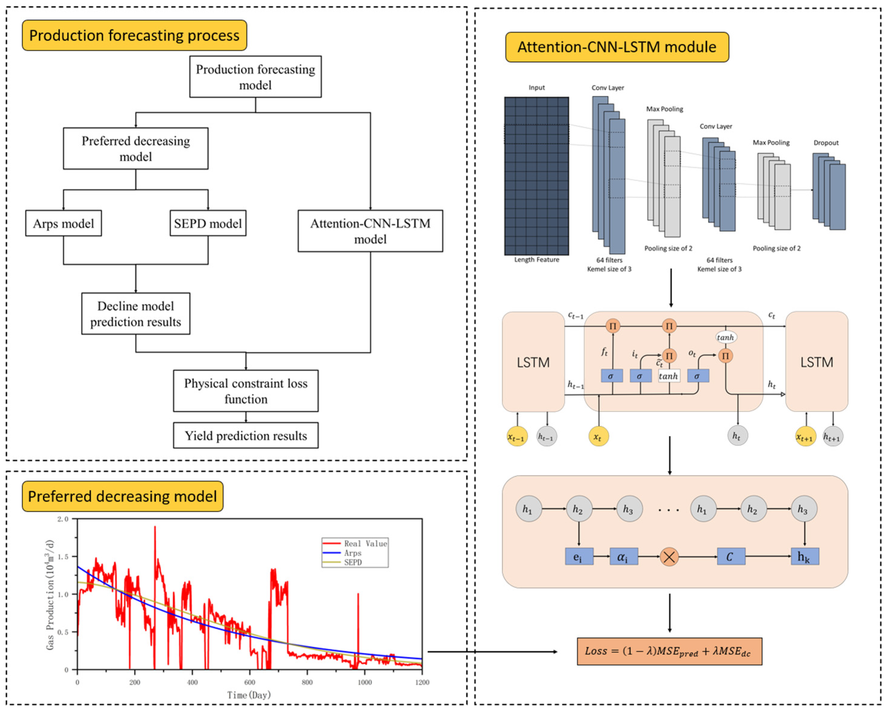
Under this background, we study and propose an intelligent production optimization strategy of “initial static similar production allocation + historical data-driven rolling production allocation”, centered on artificial algorithms, to achieve the supervision and prediction of the production operation throughout the life cycle of gas wells. The main contributions are as follows:

(1)

The local feature capture ability of CNN, the temporal dependency modeling of LSTM, and the key state focusing function of the attention mechanism are integrated to construct a deep machine learning model with multi-level features and physical constraints. The gas well decline law is embedded into the loss function to realize the joint drive of physical constraints and data of the decline curve.

(2)

An intelligent optimization production strategy of “initial static similar allocation + historical data-driven rolling allocation” is proposed. For wells in the early stage of production, based on the symmetry of production data, static production allocation is carried out by matching wells with similar geological engineering parameters through the k-nearest neighbor value algorithm. For stable production wells, the constructed machine learning model is utilized to predict short-term production, and dynamic production optimization is achieved by rolling and updating production data.

The remaining part of this article is structured as follows: Section 2 summarizes the relevant literature on the optimization methods of gas well production. The full life cycle production optimization method constructed in this paper is introduced in detail in Section 3. Section 4 conducts application tests on the constructed model. Section 5 supplements the deficiencies of the model constructed in this paper and formulates a phased intelligent optimization production strategy. Section 6 discusses the conclusion.

2. Related Works

The prediction of gas well production is an important means to determine the economic benefits of gas field development and the key to achieving the optimization of gas well production.

At present, the conventional methods for predicting the productivity of gas wells mainly include the decline curve analysis method, the analytical model method, the numerical simulation method, etc. (

Table 1. Summary table of the application of conventional gas well productivity prediction methods in oil and gas production prediction.

Method		Features
Decline curve analysis	Arps decline [8]	Suitable for conventional and tight gas reservoirs, simple calculation
	SEPD decline [9]	It is applicable to unconventional reservoirs and can fit multi-stage flows
	Duong decline [10]	It is applicable to unconventional reservoirs dominated by fractures and has a good fitting effect in the early flow stage
	Wang. et al. [11]	A SEPD + Duong hybrid model is constructed, which is applicable to production wells with rapid and unstable production declines
	Li. et al. [13]	A combined model is constructed based on linear flow model and Arps decline model
Analytical model method	Zhang. et al. [14]	Based on the superposition principle and Green’s function, a mathematical model for productivity prediction of fractured horizontal wells is constructed
	Zeng. et al. [19]	The influences of secondary fractures, permeability anisotropy and wellbore pressure drop, were taken into consideration
Numerical simulation method	Zhang. et al. [21]	The established fluid–structure coupling mathematical model was solved by using the finite element method
	Chen. et al. [23]	Considering the matrix, natural fractures, and induced fractures comprehensively, a three-dimensional seepage numerical model is established based on the finite volume discretization method
Machine learning	Liu. et al. [24]	Integrate the changing trends of the petroleum production sequence and environmental information
	Yang. et al. [25]	Multi-scale modeling
	Han. et al. [26]	Construct physical boundary conditions
	Zha. et al. [27]	Realize recursive prediction of oil and gas production
	Yildirim. et al. [28]	Consider multi-stage production prediction under physical constraints
	Shadfar. et al. [29]	Combine multiple methods and complement each other’s advantages

). The decline curve analysis method is based on the statistical law that output decreases over time. It fits historical production data through a mathematical model and extrapolates future output [6]. According to different restrictions, researchers constructed a variety of decreasing models, such as Arps decreasing, SEPD decreasing, Duong decreasing, and their combination models [7,8,9,10,11,12,13]. This method is simple to calculate, does not rely on complex geological parameters, and only requires production data over a relatively long period of time. However, due to the neglect of transient flow, it may not accurately reflect the actual production characteristics of the gas reservoir. Based on the theory of percolation mechanics, the analytical model method establishes the productivity equation, and calculates the productivity under the conditions of single-phase flow, unsteady seep flow, double hole, and double seep through the formation parameters and pressure data [14,15,16,17,18,19,20]. This method has strict requirements for assumption conditions and is difficult to handle due to complex boundary conditions. Therefore, it has limitations in some practical applications. The numerical simulation method discretizes the seepage equation by means of the finite difference method or the finite element method to solve the numerical model and achieve the production capacity prediction under conditions such as multiphase flow and multiple seepage [21,22,23]. Although this method can accurately simulate the actual complex seepage process, it requires a large amount of input data, which limits its large-scale application to a certain extent.

In recent years, the machine learning method has been widely used in gas well productivity prediction, which is realized by mining features from a large number of data [30]. According to the different research objects, machine learning capacity prediction methods can be divided into static capacity prediction and dynamic capacity prediction. Static productivity prediction is used to predict the productivity of a well at a certain stage by collecting and integrating the geological factors, engineering factors, and production dynamic factors of multiple wells. Dynamic productivity prediction takes the historical production data of production wells as input parameters and conducts time series productivity prediction through data fusion and enhancement. Liu [31] comprehensively considered geological parameters and fracturing construction parameters, and applied multiple machine learning algorithms to construct a productivity prediction model for gas wells, achieving rapid prediction based on data. Liu [32] comprehensively considered the constraints, such as geological factors, engineering factors, and production factors, and established a production prediction model through a deep learning feedforward neural network, with a predicted relative error of 5.02%. Han [26] proposed a coupling prediction method of production decline and the LSTM model. Taking the fitting error of the conventional decline analysis method and production data as the input of the LSTM model, the error was trained and coupled with the conventional decline analysis method to obtain the production prediction result, effectively reducing the prediction error of the conventional decline model. Zha [27] took the recovery rate, the number of production wells, the water production of gas wells, and the water–gas ratio as input features, and realized the monthly production prediction of gas fields through the CNN-LSTM model. In the model training, the last part of the training set was used as the unknown data of the test set to achieve recursive prediction, effectively improving the accuracy of the model. Han [33] established a physical information neural network based on domain decomposition, using sparse production data for large-scale reservoir numerical simulation. The model retained the physical continuity of the pressure gradient in the processing area and achieved strict constraints on data matching and boundary conditions.

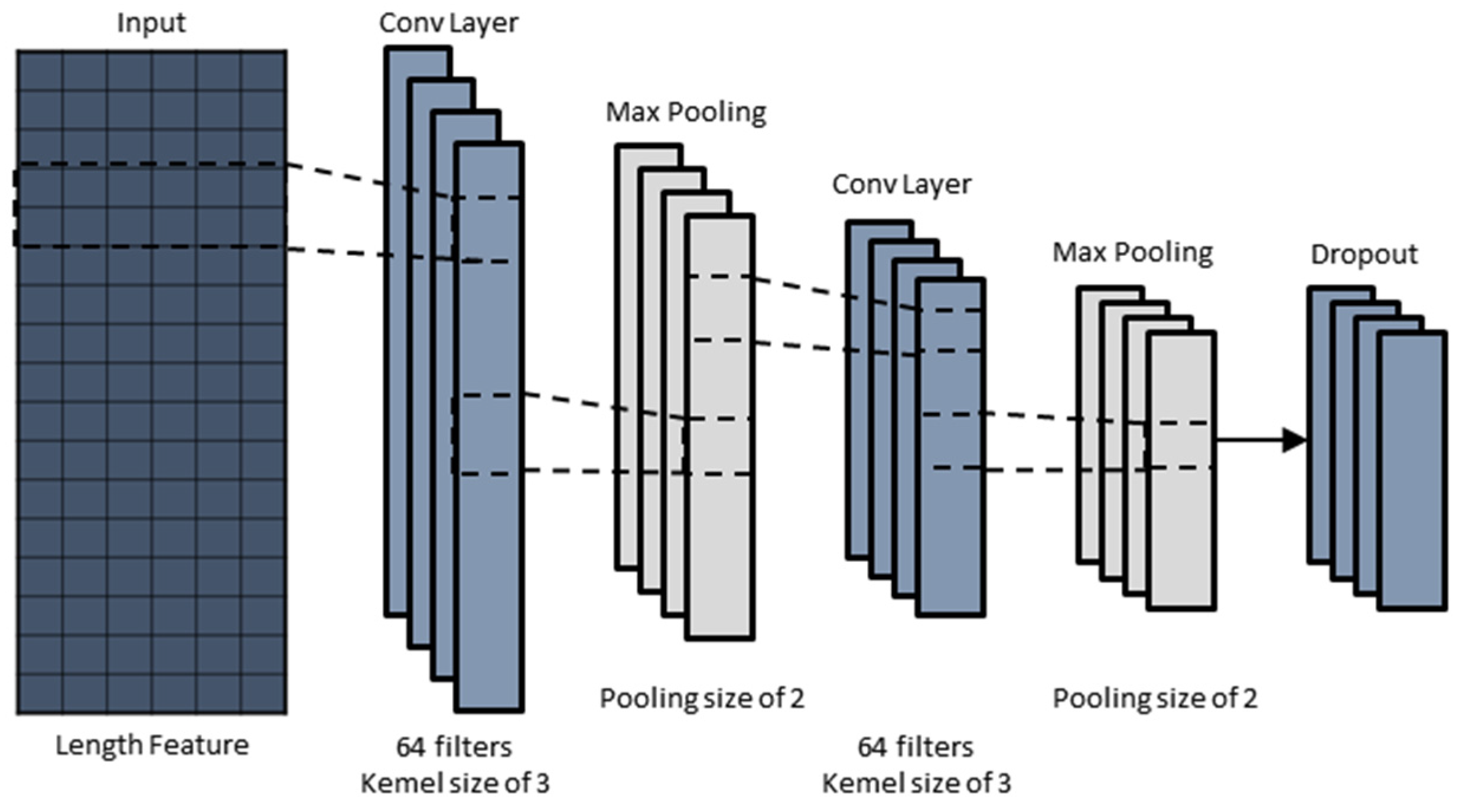
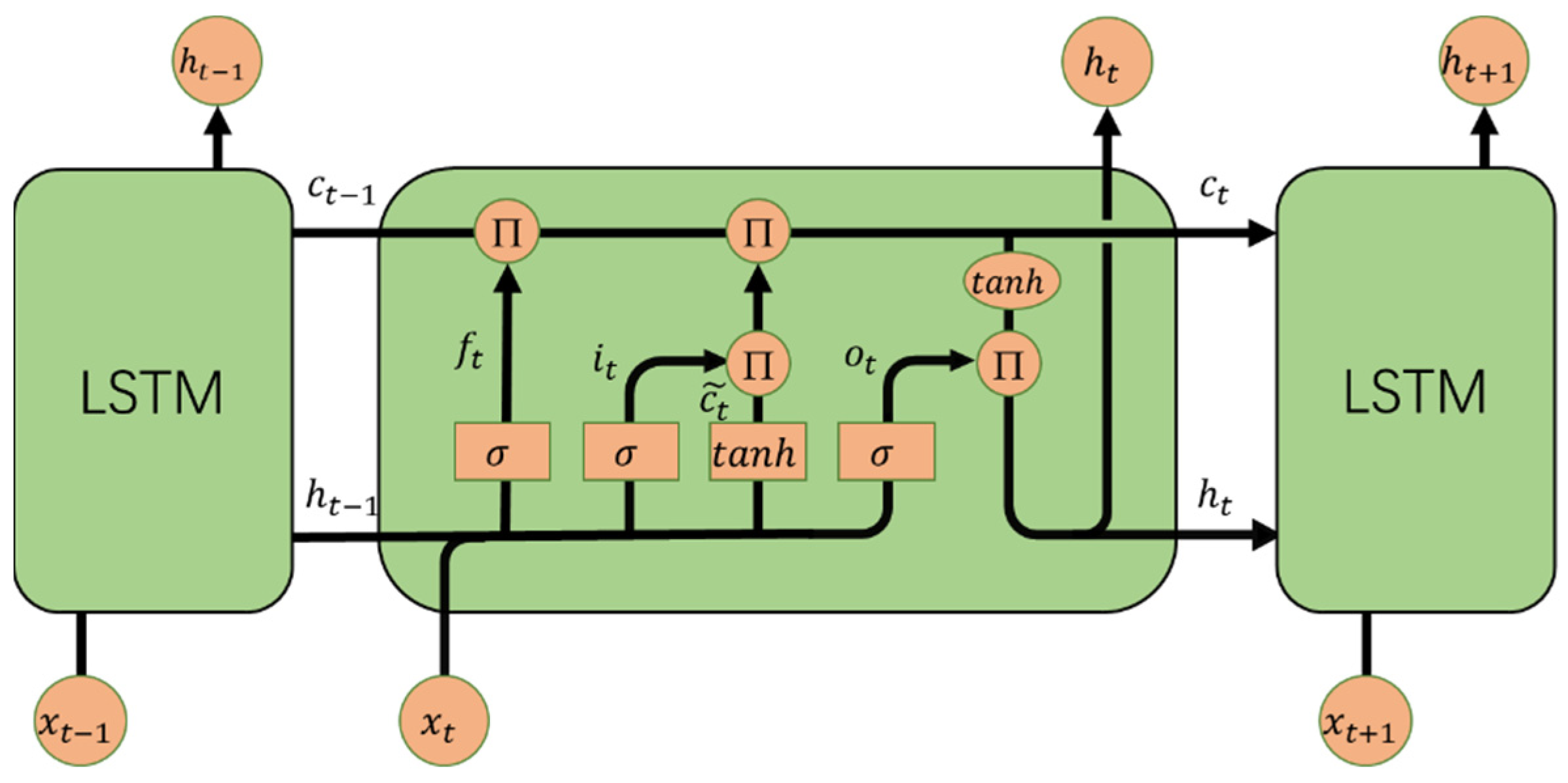
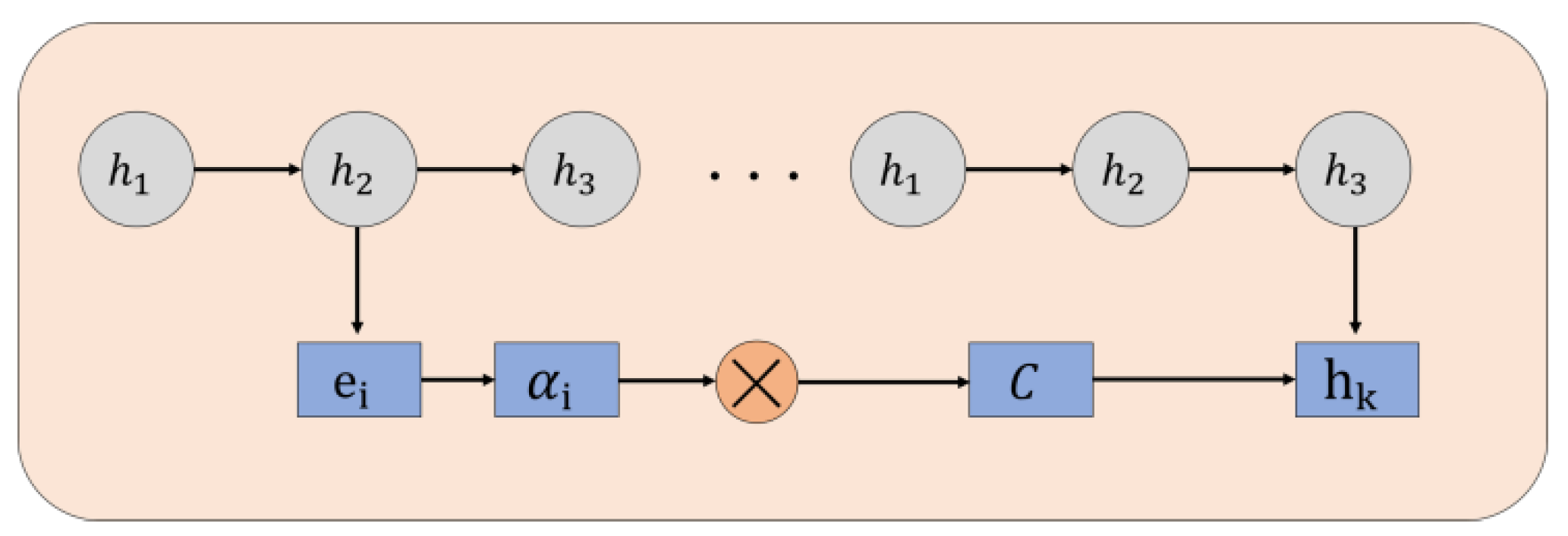
Based on the above research and analysis, the existing methods for predicting the productivity of gas wells each have their advantages and disadvantages. Conventional methods for predicting the productivity of gas wells have different types of limitations. The machine learning method achieves production prediction by mining features from a large amount of data, but the prediction results lack physical interpretability. To solve these problems, this study proposes corresponding solutions. This study integrates the local feature capture ability of CNN, the temporal dependence modeling of LSTM, and the key state focusing function of the attention mechanism to construct a multi-level feature learning system. Moreover, the decrement law of gas wells is embedded in the loss function to achieve the joint drive of physical constraints and data of the decline curve.

3. The Attention-CNN-LSTM Model Integrating Physical Constraints

This study aims to improve the accuracy of productivity prediction for tight gas wells by constructing a CNN-LSTM-attention hybrid prediction model integrating physical constraints (referred to as the P-C-L-A model). The model integrates the local feature capture capability of CNN, the time series dependency modeling of LSTM, and the key state focusing function of the attention mechanism to construct a multi-level feature learning system. It also empresses the law of gas well decline into the loss function to ensure that the prediction results conform to the principles of oil and gas reservoir engineering and break through the “black box” limitation of pure data-driven models. This model is based on the python programming language and takes the dynamic production data of a single well as input. Firstly, the production data are subjected to a decreasing fitting method to optimize the decreasing method. Secondly, the input data are trained through the attention-CNN-LSTM model (referred to as the C-L-A model). Finally, the decreasing model obtained through fitting is integrated into the loss function to physically constrain the production prediction model (Figure 1). This section elaborately introduces the fundamental principles and methods of the hybrid prediction model framework.

3.1. CNN

A convolutional neural network (CNN) is a class of feedforward neural networks that includes convolutional computation. It has the characteristics of sparse connection and weight sharing. It can effectively capture the local and global features of the data volume [34]. The main structure of CNN includes the input layer, hidden layer, and output layer, where the hidden layer is composed of a convolution layer, pooling layer, and fully connected layer. One-dimensional structures are often used to deal with time series or regression problems, as shown in Figure 2.

3.2. LSTM

A long short-term memory neural network (LSTM) is a variant of recurrent neural network (RNN) which is composed of an input layer, LSTM layer, and output layer. The LSTM layer includes a memory unit and three gating mechanisms: forget gate, input gate, and output gate [35]. The LSTM recurrent neural network structure diagram is shown in Figure 3, which is able to capture and exploit long-term dependencies in time series through memory units and gating mechanisms. In the regression problem, the gating mechanism of LSTM adaptively adjusts the transmission and forgetting of information according to the input data at each time step, effectively controlling the gradient propagation, thereby alleviating the problem of gradient disappearance and explosion.

$$f_t=\sigma \left(V_f{x}_t+W_f{h}_{t-1}+b_f\right)$$

(1)

$$i_t=\sigma \left(V_i{x}_t+W_i{h}_{t-1}+b_i\right)$$

(2)

$$\stackrel{{\displaystyle ~}}{c_t}=tanh\left(V_c{x}_t+W_c{h}_{t-1}+b_c\right)$$

(3)

$$c_t=f_t\cdot c_{t-1}+i_t\cdot \stackrel{{\displaystyle ~}}{c_t}$$

(4)

$$o_t=\sigma \left(V_o{x}_t+W_o{h}_{t-1}+b_o\right)$$

(5)

$$h_t=o_t\cdot tanh\left(c_t\right)$$

(6)

where $f_t$, $i_t$, and $o_t$ are parameters of the forgetting gate, input gate, and output gate, $\sigma$ is the sigmoid function, V and W are the weight matrices, $x_t$ is the input data at time t, $h_t$ is the output of the hidden layer, b is the linear bias of the fully connected layer, $c_t$ is the cell state parameter, and $\stackrel{{\displaystyle ~}}{c_t}$ is the input state of the memory unit. $tanh$ is a hyperbolic tangent function.

3.3. Attention Mechanism

The attention mechanism draws on the principle of human visual attention; that is, when humans observe a scene, they will not pay equal attention to all parts, but will focus their attention on certain key regions according to the task requirements. In neural networks, attention mechanisms allow the model to assign different weights to different input elements when processing input sequences, thus highlighting information that is more important to the task at hand (Figure 4).

The attention mechanism uses the weight matrix W and the nonlinear activation function (tanh) to linearly transform the state of the output value h_t of the hidden layer in the LSTM:

$$e_t=tanh\left(W\cdot h_t\right).$$

(7)

The normalized weight ${\alpha }_t$ is further calculated by the softmax function:

$${\alpha }_t={\displaystyle \frac{exp\left(e_t\right)}{{{\displaystyle \sum }}_{i=1}^{T}exp\left(e_i\right)}}.$$

(8)

Using the calculated attention weights, the hidden states of the LSTM output are weighted and summed to obtain the weighted feature vector C:

$$C={\displaystyle \sum }_{t=1}^T{\alpha }_t{h}_t.$$

(9)

3.4. Physical Constraints

In recent years, with the in-depth research and application of machine learning methods in oil and gas fields, scholars tried to combine traditional production capacity prediction methods with machine learning to enhance the interpretability of data-driven models through physical constraints, which provides new research directions for production capacity prediction. Some researchers incorporate physical constraints into machine learning models by defining loss functions. Yuan [36] combined the physical model with the deep learning model, and added physical constraints to the model prediction in the form of loss function, which enhanced the interpretability of the prediction model and improved the performance of the model after adding physical constraints. Ren [37] used a particle swarm optimization algorithm to carry out history fitting with the goal of minimum cumulative production error, established a production capacity prediction model adaptive to flow and production changes, transformed the unstable flow problem into a quasi-stable flow problem and solved it, and simplified the impact of reservoir heterogeneity, and the production capacity prediction model had stable performance and high accuracy in long-term prediction.

In the actual productivity prediction task, due to the difference of reservoir geological characteristic parameters between wells and the missing data of some wells, it is difficult to directly integrate physical constraints into the loss function for the percolation differential equation. In order to solve this problem, based on the symmetry of historical production data and the decline model, this study uses the historical data to select the best decline model. The fitting decline equation is embedded in the loss function in the form of regularization, and the weighted coefficient is used to balance the data-driven and physical constraints so that the model can effectively constrain the production decline trend in the training process. This will enhance the accuracy and stability of the prediction results.

3.4.1. Principle of Decline Model

As the study area is a tight sandstone gas reservoir, the reservoir permeability is low and the heterogeneity is strong. Taking into account the characteristics of various conventional decrement methods comprehensively, among them, the Arps decrement model is flexible in application and can handle changes at different decrement stages, while the SEPD decrement model has better adaptability to complex flow mechanisms. Therefore, the Arps decreasing model and the SEPD decreasing model are selected for detailed analysis and serve as the physical constraints of the capacity prediction model in this paper.

The Arps decline model was proposed by J.J. Arps in 1945 and is widely used in the analysis of production decline in both conventional and unconventional oil and gas reservoirs. This model describes the law of production decline of oil and gas wells over time through mathematical formulas and is used to predict future production capacity and single-well reserves. Its general formula is as follows:

$$q_n={\displaystyle \frac{q_i}{{\left(1+b{D}_{i}t\right)}^{1/b}}}$$

(10)

where $q_n$ is the daily gas production at the gas well time n (n = 0, 1, 2, … , N); $q_i$ represents the initial gas production; $D_i$ is the initial decline rate; and $b$ is the decreasing index.

The Arps decline model classifies production decline into three types based on the difference in the decline index n: exponential decline (b = 0), hyperbolic decline (0 < b < 1), and harmonic decline (b = 1).

The extended exponential decline model (SEPD) was proposed by Valko. This model can not only be used for the analysis of the decline pattern of production data in shale gas wells, but is also applicable to the analysis of the decline pattern of production data in tight gas wells. The SEPD model uses exponential decline to describe the “flat tail” stage in the later stage of gas well production:

$${\displaystyle \frac{dq}{dt}}=-n{\left({\displaystyle \frac{t}{t}}\right)}^n{\displaystyle \frac{q}{t}}$$

(11)

where $\tau$ is the characteristic relaxation time of the model, d; $n$ is the dimensionless time exponent.

The daily gas production $q$ can be written as follows:

$$q=q_i\mathit{exp}\left[-{\left({\displaystyle \frac{t}{\tau }}\right)}^n\right].$$

(12)

The SEPD decrement method and the Arps exponential decrement method are extremely similar. The difference lies in that the former regards the decrement index as constantly changing, while the latter regards it as constant. The Arps decreasing model is only applicable to the production data analysis in the boundary control flow stage, while the SEPD decreasing model can be applied to the unstable flow and transitional flow production stages.

3.4.2. Physical Constraint Embedding Mechanism

Take the Arps hyperbolic decreasing model as an example, its expression is as follows:

$$q_n={\displaystyle \frac{q_i}{{\left(1+b{D}_{i}t\right)}^{1/b}}}.$$

(13)

Suppose the output prediction of the C-L-A model at time step n is as follows:

$${\widehat{q}}_n=f_{\theta }\left(X_n\right)$$

(14)

where $f_{\theta }$ is the C-L-A model with parameter $\theta$; $X_n$ is the input feature of time step n.

During the training process of the model, the hyperbolic decreasing constraint is added to the loss function, and the calculation formula is as follows:

$$Loss=\left(1-\lambda \right)MS{E}_{pred}+\lambda MS{E}_{dc}$$

(15)

$$MS{E}_{pred}={\displaystyle \frac{1}{N}}{\sum }_1^N{({\widehat{q}}_n-q_n^{\prime })}^2$$

(16)

$$MS{E}_{dc}={\displaystyle \frac{1}{N}}{\sum }_1^N{(q_n-q_n^{\prime })}^2$$

(17)

where ${\mathit{MSE}}_{\mathit{pred}}$ is the mean square error between the real data and the predicted data of the C-L-A model. ${\mathit{MSE}}_{\mathit{dc}}$ is the mean square error between the real data and the predicted data of the decrement constraint model. $q_n^{\prime }$ represents the actual output data, and $\lambda$ is the weighting coefficient for balancing data fitting and physical constraints (0 ≤ $\lambda$ ≤ 1). In this chapter, $\lambda$ is taken as 0.6.

4. Model Application Testing

We test the application of the model constructed in this paper in this section. In the experiment, firstly, the influence of adding physical constraints on the performance of the model was analyzed. Secondly, ablation experiments were carried out to verify the importance of each module in the model. Similarly, we compare the proposed model with conventional machine learning algorithms to verify the advancement of the proposed model. Meanwhile, considering that the model input is multi-parameter, we analyze the contributions of different physical parameter constraints to the model. Finally, the weight factor in the loss function is set to determine the balance point between the best physical constraint and the data fitting.

4.1. Data Collection and Experimental Setup

4.1.1. Data Collection

All the data in the article are from the eastern area of the Sulige gas field in the Ordos Basin. This gas field is a typical tight sandstone gas reservoir with low pressure, low permeability, low abundance, river sand bodies as the main body, and large areas of reservoirs distributed [38]. In this section, the dynamic production data of tight gas wells with different commissioning times in the study area are selected as the research objects, including six dynamic characteristics such as casing pressure, tubing pressure, production time, daily water production, and daily gas production.

Due to the different dynamic characteristic parameter units of gas wells, the numerical differences among them are large, which affects the convergence speed of model training. Therefore, here, deviation standardization is selected to map the data to the range of [0, 1], adjusting the numerical range between different features or different samples to a relatively consistent level, eliminating the influence of dimensions among various feature parameters, and reducing the problems of vanishing or exploding gradients in machine learning. Its normalization formula is shown in Equation (18).

$$X^{\prime }={\displaystyle \frac{X_i-X_{min}}{X_{max}-X_{min}}}$$

(18)

where $X^{\prime }$ is the normalized data; $X_{\max }$ and $X_{\min }$ are the maximum and minimum values of the input dataset $X_i$.

4.1.2. Model Evaluation Index

To evaluate the performance of the established tight gas well production prediction model, this paper uses mean absolute error (MAE) and root mean square error (RMSE) to assess the error of the prediction model.

$$MAE={\displaystyle \frac{1}{n}}{\displaystyle \sum }_{i=1}^n\left|f\left(x_i\right)-x_i\right|$$

(19)

$$RMSE=\sqrt{{\displaystyle \frac{1}{n}}{\displaystyle \sum }_{i=1}^n{\left(f\left(x_i\right)-x_i\right)}^2}$$

(20)

where $f\left(x_i\right)$ is the predicted value of daily gas production per well and $x_i$ is the real value.

4.1.3. Model Parameter Settings

The model is successively composed of the CNN module, the LSTM module, and the attention mechanism layer in series, and uses the decreasing model as the physical constraint embedding loss function. Considering the influence of model parameters on model performance, the grid search method is used to optimize hyperparameters.

Table 2. Hyperparameter search range.

Model Name	Hyperparameters	Search
CNN	Number of convolutional layers	[1, 2, 3]
	Number of convolution kernels	[16, 32, 64, 128]
	Convolution kernel size	[2 × 1, 3 × 1, 5 × 1]
LSTM	Number of LSTM layers	[1, 2, 3]
	Number of neurons in the hidden layer	[64, 128, 256]
	Dropout	[0.1, 0.2, 0.3, 0.5]
Training configuration	Epochs	[500, 1000, 1500]
	Number of iterations per round	[3, 5, 10]
	Initial learning rate	[0.001, 0.01, 0.1]

shows the search range of hyperparameters.

Firstly, based on the daily gas production data, hyperbolic decreasing curves and SEPD decreasing curves are, respectively, fitted. Through comparative analysis, the curve-fitting method with a higher degree of fitting is selected and integrated as a physical constraint into the subsequent model loss function.

Divide the input data into a training set and a test set in a 7:3 ratio. The CNN neural network is used to interconnect the features of the input data and learn the spatial features of the data set. In the CNN module, the number of convolutional layers is determined to be two through the grid search method. The number of convolutional kernels in the first and second layers is 32 and 64, respectively, and the size is 3 × 1. The activation function selects the Relu function and adopts a 2 × 1 max pooling layer for dimensionality reduction.

The output data of the CNN layer are re-expanded through the sequence expansion layer as the input data of the LSTM layer. The LSTM module is used to further extract the temporal features of the data. The number of LSTM layers is determined to be 2 and the number of hidden neurons is 128 through grid search. At the same time, a dropout layer is introduced after the LSTM module, with the dropout rate set at 20% to prevent overfitting.

The weights of the attention mechanism are adaptively adjusted by averaging the input feature map in the spatial dimension and then processing it with the Softmax function.

The model training cycle is determined to be 1000 rounds through grid search, with three iterations in each round. The initial learning rate is 0.01, and the optimizer uses the Adam gradient descent algorithm.

4.2. Analysis of the Performance Results of the Physical Constraint Model

In this section, the dynamic production data of four tight gas wells with different production times in the study area are selected as the research objects. By comparing and analyzing the fitting effects of the Arps hyperbolic decrement model and the SEPD decrement model, the optimal decrement model is chosen as the physical constraint, and the CNN-LSTM-attention data-driven model is combined for production capacity prediction.

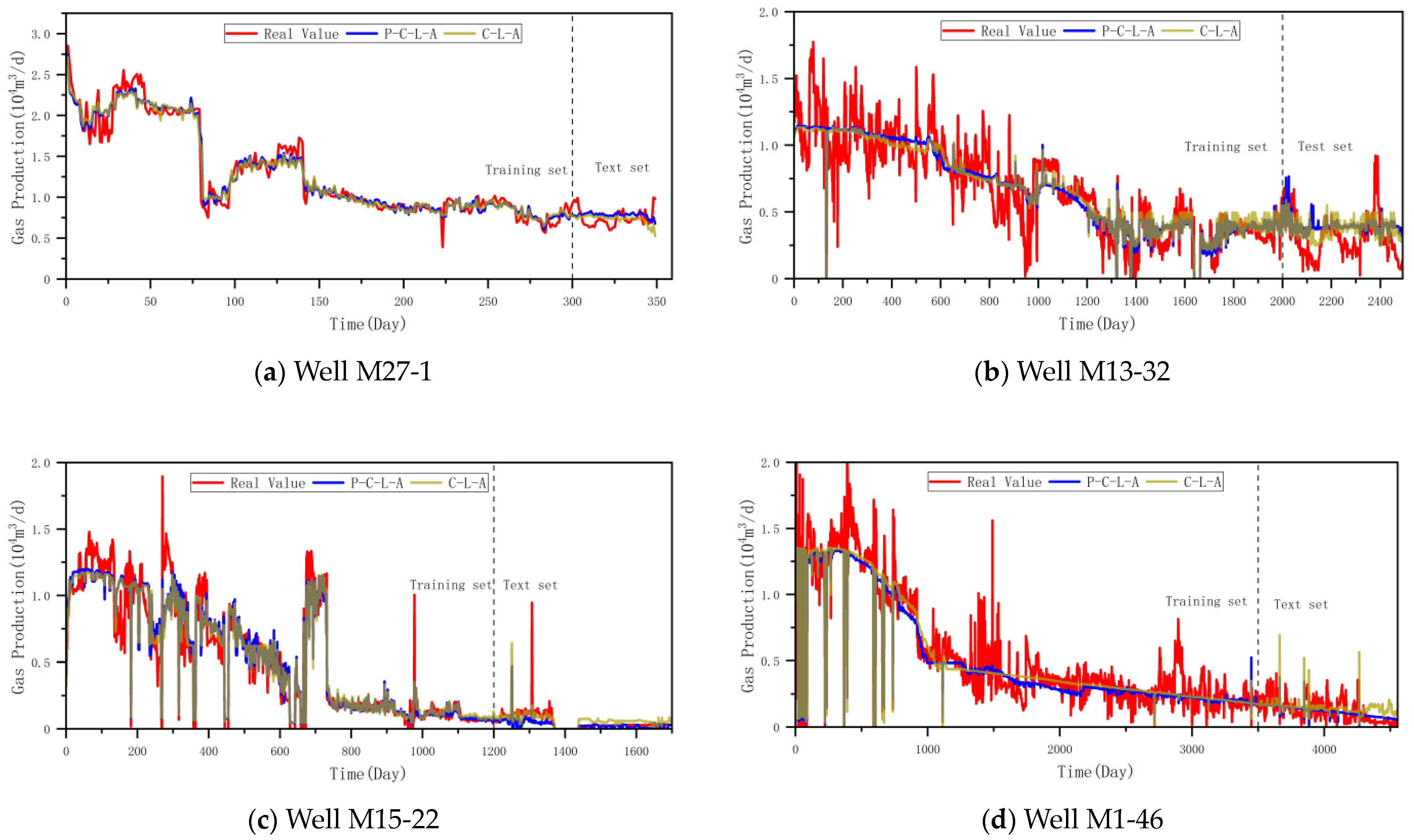
By comprehensively comparing the prediction effect diagrams of the four wells, it is found that the C-L-A model without physical constraints has significant production fluctuation with the increase in prediction time, while the integration of physical constraints can effectively suppress this phenomenon, and the prediction results are closer to the real data (

Table 3. Comparison table of influence of physical constraints on model error (obtained by running each method 20 times).

Well	Model		MAE (104 m3)	RMSE (104 m3)
M27-1	P-C-L-A	Training	0.0834	0.1221
		Test	0.1018	0.1177
	C-L-A	Training	0.0855	0.1250
		Test	0.0938	0.1261
M13-32	P-C-L-A	Training	0.0966	0.1431
		Test	0.0499	0.0651
	C-L-A	Training	0.0975	0.1443
		Test	0.0644	0.0827
M15-22	P-C-L-A	Training	0.0918	0.1405
		Test	0.0274	0.0552
	C-L-A	Training	0.0899	0.1383
		Test	0.0296	0.0573
M1-46	P-C-L-A	Training	0.1212	0.1597
		Test	0.1321	0.1571
	C-L-A	Training	0.1226	0.1621
		Test	0.1437	0.1768

). As can be seen from the comparison figures of prediction errors of different wells (Figure 5), after embedding the decreasing law as a physical constraint into the C-L-A model, the accuracy of the model is further improved, and the root mean square error and the mean absolute error are both less than 0.20 × 10⁴ m³, showing good performance in dealing with the productivity prediction problem of tight gas wells.

4.3. Ablation Experiment

In order to evaluate the sensitivity of the combined model to data input and the influence of different modules on the model performance, ablation experiments were conducted on the CNN-LSTM-attention data-driven model based on physical constraints. The specific method is to remove the physical constraints, attention module, LSTM module, and CNN module in the model in sequence. The errors of the ablation experiment results are shown in

Table 4. Comparison table of ablation experiments (obtained by running each method 20 times).

Model		MAE (104 m3)	RMSE (104 m3)
P-C-L-A	Training	0.0835	0.1222
	Test	0.0999	0.1195
C-L-A	Training	0.0855	0.1250
	Test	0.1049	0.1211
CNN-LSTM	Training	0.0924	0.1316
	Test	0.1169	0.1303
LSTM	Training	0.0958	0.1326
	Test	0.0972	0.1318
CNN	Training	0.1523	0.1991
	Test	0.1440	0.1578

.

After removing the physical constraints, all evaluation indicators of the C-L-A model showed a significant downward trend compared with the complete model. The mean absolute error increased by 0.005 × 10⁴ m³ and the root mean square error increased by 0.0016 × 10⁴ m³. To verify the statistical significance of this difference, t-tests were conducted on the mean absolute error and root mean square error of the two test sets, respectively. The results show that the corresponding p-values were 0.041 and 0.045, respectively, both less than the significance level of 0.05, indicating that the degradation in model performance caused by the removal of physical constraints was statistically significant. Physical constraints provide the model with the fundamental decreasing law of gas well production. After incorporating physical constraints, the model can learn data features more efficiently, reduce overfitting phenomena, and enhance the generalization ability of the model.

After further removing the attention mechanism, the performance of the CNN-LSTM model significantly declined in various indicators, with the mean absolute error increasing by 0.0169 × 10⁴ m³ and the root mean square error increasing by 0.0109 × 10⁴ m³. Significance tests were conducted on the test set indicators of this model and the C-L-A model. It was found that the p-values of the t-tests for the mean absolute error and the root mean square error were 0.023 and 0.028, respectively, both being less than 0.05, indicating that this performance degradation was statistically significant. When dealing with abnormal fluctuation data caused by special circumstances, such as well closure and well repair during the gas well production process, the attention mechanism can accurately identify and filter out this interfering information, enabling the model to focus more on the core and valuable data features. This greatly enhances the model’s ability to interpret data and ensures that the model outputs more accurate and reliable prediction results.

Compared with the complete model, the performance indicators of the LSTM model significantly declined, with the mean absolute error increasing by 0.0033 × 10⁴ m³ and the root mean square error increasing by 0.0124 × 10⁴ m³. Significance analysis of the test set data of the LSTM model and the CNN-LSTM model showed that the p-value of the t-test for the mean absolute error was 0.037, and the p-value of the t-test for the root mean square error was 0.031, both of which were less than 0.05, indicating that the difference between the two was statistically significant. This result confirms the significance of the convolutional module, which is responsible for extracting spatial features such as pressure and water production from production data. The absence of this module can have a significant impact on model performance.

The performance indicators of the CNN model decreased the most severely, with the mean absolute error increasing by 0.0441 × 10⁴ m³ and the root mean square error increasing by 0.0383 × 10⁴ m³. Significance tests were conducted on the test set performance of the CNN model and the LSTM model. It was found that the p-values of the t-tests for the mean absolute error and the root mean square error were 0.006 and 0.005, respectively, both of which were much less than 0.05, indicating that the performance difference between the two was statistically extremely significant. This further confirms the crucial role of the long short-term memory neural network module in model performance. This module can capture more accurate yield timing patterns, and its absence would lead to a significant decline in model performance. This further confirms the crucial role of the long short-term memory neural network module in model performance. This module can capture more accurate yield timing patterns, and its absence would lead to a significant decline in model performance.

The results of the ablation experiment show that each module contributes to the model performance. The CNN-LSTM-attention data-driven model based on physical constraints established in this paper performs the best in various performance indicators. The physical constraints based on the decreasing analysis method provide a reasonable initial value for the model, and the attention mechanism filters out the redundant features in the production data. The convolutional neural network module focuses on spatial features such as pressure, daily water production, and well opening time, while the long short-term memory neural network module captures the changing trend of production over time. The above experimental results verify that the model proposed in this paper, through the combination of physical constraints, attention mechanisms, convolutional neural networks, and long short-term memory neural networks, achieved a relatively good prediction of the productivity of tight gas wells, and the roles of each component are all significant.

4.4. Comparative Test

To verify the performance of the CNN-LSTM-attention data-driven model based on physical constraints in this paper, comparative experiments were conducted using random forest, support vector machine, linear regression, and BP neural network models, respectively.

As can be seen from

Table 5. Comparison experiment comparison table (obtained by running each method 20 times).

Model		MAE (104 m3)	RMSE (104 m3)
P-C-L-A	Training	0.0835	0.1222
	Test	0.1018	0.1177
Random forest	Training	0.1189	0.1562
	Test	0.1400	0.1732
SVM	Training	0.1961	0.2533
	Test	0.2300	0.3000
Multiple linear regression	Training	0.2006	0.2457
	Test	0.2200	0.2739
BP	Training	0.0988	0.1404
	Test	0.1100	0.1549

, on the tight gas well productivity prediction task, the performance index of the CNN-LSTM-attention data-driven model based on physical constraints in this paper performs the best, and the accuracy of the prediction results is better than other models. Compared with the suboptimal BP neural network, the root mean square error is reduced by 24.41%. The CNN-LSTM module in the model of this paper has a better ability of spatio-temporal feature fusion.

Random forest is good at capturing nonlinear relationships, but its ability to fit the long-term trend of a time series is weak in the task of gas well productivity prediction. The root mean square error is 27.82% higher than that of the model proposed in this paper.

The performance parameters of the support vector machine and multiple linear regression in the comparative experiments were relatively poor. Among them, the mean absolute error was 0.1961 × 10⁴ m³, and the root mean square error was 0.2533 × 10⁴ m³. The mean absolute error is 0.2006 × 10⁴ m³, and the root mean square error is 0.2457 × 10⁴ m³. Compared with the CNN-LSTM-attention data-driven model based on physical constraints, the support vector machine and the multiple linear regression model have obvious deficiencies in capturing the characteristics of a time series. It is difficult to effectively handle the dynamic characteristics of gas well production data changing over time and we cannot fully explore the potential patterns in the data. This leads to the poor accuracy and stability of the prediction results.

The superiority of the CNN-LSTM-attention data-driven model based on physical constraints in the productivity prediction task of tight gas wells has been fully verified through comparative experiments, providing a more accurate and reliable method for the productivity prediction of tight gas wells.

4.5. Contributions of Different Physical Parameter Constraints

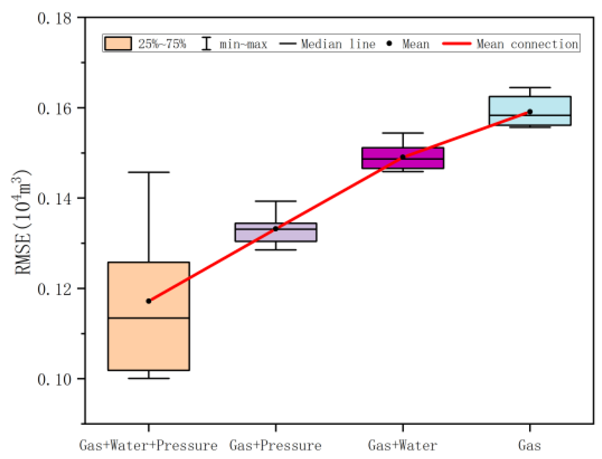
Since the decline of gas production in gas wells is closely related to wellhead pressure and water production, it is necessary to consider the influence of wellhead pressure and water production on gas production. Therefore, the six input characteristic parameters of casing pressure, tubing pressure, production time, daily water volume, and daily gas volume are divided into wellhead pressure (casing pressure and tubing pressure), gas production (production time and daily gas volume), and water production (daily water volume). Figure 6 to Figure 7 compare the prediction performance of different physical parameters on the model.

It can be seen from the figure that wellhead pressure and water production have different degrees of improvement on model performance, and wellhead pressure has the greatest impact on model performance, followed by water production, and when only gas production is considered, the model performance is the worst, which indicates that different physical parameter constraints can reduce model prediction errors from different angles, thereby improving the stability and accuracy of production prediction.

4.6. Comparison of Weighting Factors

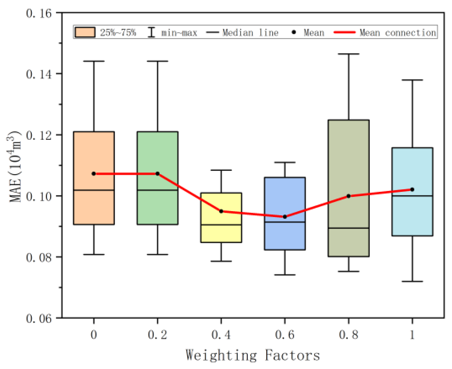
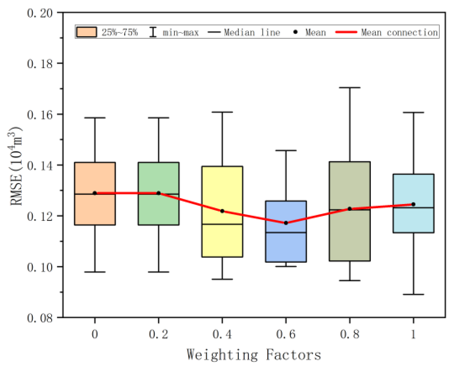
The weighting factor $\lambda$ in the loss function is a weight coefficient that balances data fitting and physical constraints, significantly affecting the performance of the production prediction model. To study the influence of weighting factors on the model, a comparative experiment was conducted on 10 wells with different $\lambda$, while the other parameters of the model remained unchanged. Figure 8 and Figure 9 show the performance errors of the model when the weighting factors $\lambda$ are 0, 0.2, 0.4, 0.6, 0.8, and 1, respectively.

It can be seen from the figure that with the increase in the weighting factor, MAE and RMSE show a trend of first decreasing and then increasing. When $\lambda$ increases from 0 to 0.2, the average values of RMSE and MAE remain unchanged (RMSE = 0.12891, MAE = 0.10723), indicating that the physical constraint weights within this interval are too low. The model is almost completely data-driven, and minor adjustments to $\lambda$ have no significant impact on performance. At this time, the model is dominated by data fitting. When $\lambda$ increased from 0.2 to 0.6, the error index continued to decrease as $\lambda$ increased, and the decrease gradually narrowed. RMSE decreased from 0.12891 to 0.11715 (a decrease of 9.1%), and MAE decreased from 0.10723 to 0.09315 (a decrease of 13.1%). The effect of physical constraints decreases as $\lambda$ increases. At this stage, physical constraints gradually strengthen, form synergy with data fitting, and the model performance gradually improves. When $\lambda$ exceeds 0.6, the error index shows an upward trend as $\lambda$ increases. At this time, the physical constraints of the model and the data fitting are out of balance. Excessive physical constraints weaken the adaptive advantage of the model’s data fitting, making it impossible to capture the nonlinear features in the production data, and the model performance gradually deteriorates. When $\lambda$ = 0.6→0.8, RMSE increases by 4.8% and MAE increases by 7.3%. When $\lambda$ = 0.8→1, RMSE increases by 1.4% and MAE increases by 2.2%.

$\lambda$ = 0.6 is the optimal sensitive point for model performance. At this point, both RMSE and MAE reach their minimum values, and a precise balance is achieved between physical constraints and data fitting. When the value is lower than this, the increase in $\lambda$ has a significant effect on improving the performance of the model. When the value is higher than this, the increase in $\lambda$ has a negative impact on the performance of the model. In the practical application of gas wells in the Sulige gas field, setting the weighting factor to 0.6 ± 0.05 can maximize the advantages of the model and assist in the decision-making of gas field development. For other gas fields, the sensitivity analysis of weighting factors should be reconducted, and the reasonable weighting factors should be re-determined to improve the universality of the model.

5. Intelligent Production Optimization of Tight Gas Wells

Considering that there is less production data in the early stage of production well commissioning, there may be deviations in the prediction error when directly using the physical constraint model established in this paper for production allocation. To this end, the production wells are divided into the production wells in the initial stage of production and the stable production wells. Dynamic optimization methods are formulated in stages to achieve dynamic optimized production throughout the entire life cycle of gas wells.

For the early production wells, based on the symmetry of the data, the initial working system and dynamic and static parameters of the production wells are taken as the data support, and the geological, engineering, and dynamic factors are comprehensively considered. The K-nearest neighbor algorithm (KNN) is used to search the data of similar wells in the production wells, and the initial allocation of similar wells is used to guide the target wells to determine a reasonable working system.

For the stable production wells, the CNN-LSTM-attention data-driven productivity prediction model with physical constraints established in Section 4 is used for production allocation. By comparing the model performances of different prediction durations and well shutdown times, the production of gas wells in the study area is optimized according to the production dynamics.

5.1. Production Wells in the Initial Stage of Production

In the early stage of production, the production data of the production wells are relatively small. When the physical constraint model established in this paper is directly used for optimized production, there may be deviations in the prediction errors. In this paper, through the K-nearest neighbor value algorithm, reasonable action systems are formulated for new wells based on the dynamic and static data of trial production and production systems of the wells that have been put into production, and the production allocation prediction of new wells is achieved through data-driven approaches.

The specific production allocation ideas are as follows:

Step 1: Collect the dynamic and static parameters of the wells that have been put into production and the new wells to be allocated to production and construct a multi-dimensional feature matrix.

Step 2: The dynamic and static parameters of the wells put into production are normalized, and the Pearson correlation coefficient is used to quantify the correlation between each characteristic parameter and the production volume. The CRITIC weight analysis method is adopted to calculate the weights of the characteristic parameters. This method is an objective weighting method based on the data themselves, and the weights are determined by comprehensively considering the variability of the indicators and the conflict between the indicators. The specific steps are as follows:

Calculate the standard deviation among the parameters and measure the contrast intensity within each index:

$${\sigma }_j=\sqrt{{\displaystyle \frac{1}{n}}{\displaystyle \sum _{i=1}^n{(x_{ij}-{\overline{x}}_j)}^2}}.$$

(21)

The coefficient is used to measure the information conflict between indicators, where $r_{jk}$ is the Pearson correlation coefficient between indicators j and k:

$$f_j={\displaystyle \sum _{k=1}^m(1-r_{jk})}.$$

(22)

Calculate the amount of information of the indicators through the standard deviation and conflict of the indicators:

$$C_j={\sigma }_j\times f_j.$$

(23)

Calculate the weights based on the amount of indicator information:

$$w_j={\displaystyle \frac{C_j}{{\displaystyle \sum _{k=1}^m{C}_k}}}.$$

(24)

Step 3: Conduct similar well matching and production allocation prediction through the K-nearest neighbor value algorithm.

Among the wells that have been put into production, those with an effective thickness difference of no more than ±4 m from the new wells to be allocated to production are selected to form a “candidate-similar well pool”. The weighted Euclidean distance method is used to calculate the distance between the new wells to be allocated to production and the candidate wells, and the k wells with the shortest distance are selected. The formula for calculating the weighted Euclidean distance is as follows:

$$d_{ij}=\sqrt{{{\displaystyle \sum }}_{k=1}^n{\omega }_k{\left(x_{ik}-x_{jk}\right)}^2}$$

(25)

where $d_{ij}$ is the weighted Euclidean distance, ${\omega }_k$ is the weight of the KTH parameter, $x_{ik}$ is the characteristic parameter of the KTH new well, and $x_{jk}$ is the characteristic parameter of the KTH producing well.

Take the weighted average of the initial production allocation distances of similar wells as the initial production allocation value of new wells to guide the production allocation of new wells. The formula of distance-weighted average is as follows:

$$q_{new}={\displaystyle \frac{{{\displaystyle \sum }}_{m=1}^k\frac{1}{d_m}{q}_m}{{{\displaystyle \sum }}_{m=1}^k\frac{1}{d_m}}}$$

(26)

where $q_{new}$ is the similar production to be replaced, $d_m$ is the distance between the m and $q_{new}$, and $q_m$ is the production of similar wells.

Taking well M2-45 as an example, the unobstructed flow rate calculated by the single-point method productivity test of this well is 5.64 × 10⁴ m³/d. Based on the production instability analysis and allocation of the trial production data, allocation of 2 × 10⁴ m³/d indicates stable production for 2 years and a kit pressure drop rate of less than 0.02 MPa/d. Two similar wells were found through the K-nearest neighbor algorithm, and the initial production allocation of well M2-45 was obtained as 1.77 × 10⁴ m³/d through a distal-weighted average, with a relative error of 11.5% (

Table 6. Data of similar wells in well M2-45.

Parameters	Well M2-45	Well M21-87#	Well M23-85#
initial production allocation (104 m3/d)	2.00	1.5	2.10
pre-production output (104 m3/d)	3.64	1.63	2.12
absolute open flow rate (104 m3/d)	5.64	16.23	20.96
pre-production casing pressure (MPa)	19.2	25.54	20.18
gas production per unit pressure drop (104 m3/MPa)	16.15	22.49	32.46
porosity (%)	8.75	8.08	8.82
permeability (10−3 µm2)	0.52	0.51	0.56
gas saturation (%)	65.44	63.92	59.29
cumulative effective thickness (m)	16.9	12.9	13
formation pressure (MPa)	26.02	29.32	26.32
perforation thickness (m)	6	9	6
perforated interval number (pieces)	4	3	2

In Table 6, "#" indicates similar Wells found among the production Wells that have been put into operation in the study area based on the data of the target well.

).

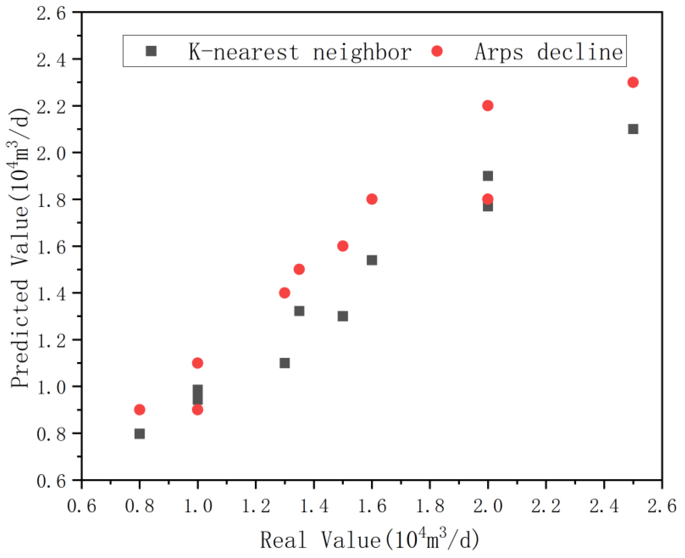
The K-nearest neighbor algorithm and the Arps decreasing method were applied to predict the initial production allocation of 10 sample wells in the study area (Figure 10). The results show that in the early stage of production with limited data, the average relative error of the K-nearest neighbor allocation method (7.45%) is lower than that of the Arps decreasing allocation method (10.1%), indicating that its predictive performance is better. This is mainly because Arps decline analysis is based on the law of production attenuation and requires certain production data support, making it more suitable for wells that already have short-term production history data. The K-nearest neighbor method does not require the production of historical data. It can predict only by relying on static parameters and well test data and is more suitable for the initial stage of new well production. Therefore, for production wells in the early stage of production, the K-nearest neighbor algorithm is mainly adopted, combined with geological thresholds to screen similar wells, to ensure the reliability of the prediction basis.

5.2. Stable Production Well

The production of gas wells tends to be stable 3 to 6 months after the production of production wells is put into operation, and there is a significant change trend in the dynamic parameters, such as gas production and casing pressure. At this time, according to the physical constraint model established in Section 4, a reasonable rolling prediction and optimization production system is formulated by comparing the model performance under different prediction time and shut-in time conditions. In order to visually demonstrate the model error, only the root mean square error is used as the evaluation index in this subsection.

5.2.1. Comparison of Different Prediction Duration Models

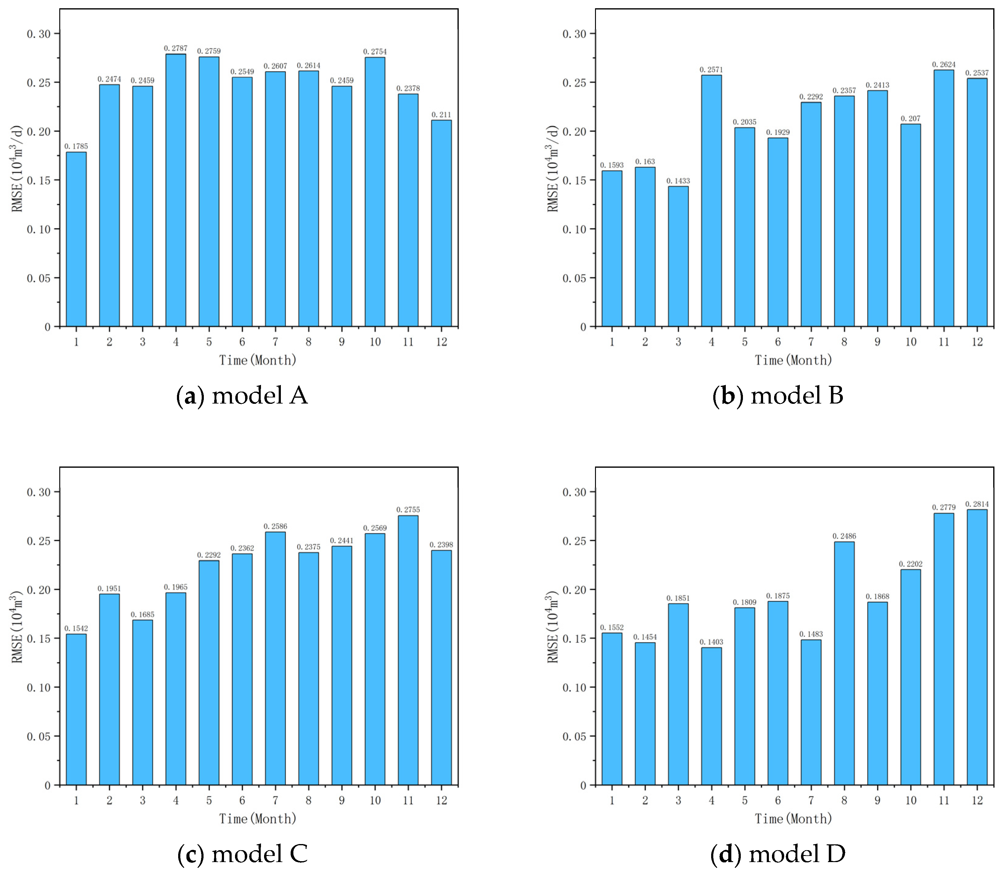
The production dynamic data of three tight gas wells in the study area were selected as the training set, and four prediction models based on 90d historical data (model A), 180d historical data (model B), 270 d historical data (model C), and 360 d historical data (model D) were established, respectively. The gas production for the next 30 to 360 days was predicted, respectively, in units of 30 days, and the prediction performance of different models for different time periods was evaluated through the root mean square error (Figure 11).

Comparing the root mean square error of the four models to predict future production in the same model, with the increase in prediction time, the root mean square error shows an upward trend to a certain extent, and the longer the model prediction time, the lower the accuracy. When predicting the gas production in the next 30 days, the root mean square error decreases with the increase in sample data, averaging 0.1618 × 10⁴ m³. The sample data provide data support for the production prediction. When the predicted production time exceeded the production time of half of the sample data, the root mean square error of the models was greater than 0.2 × 10⁴ m³. Among the four models, model D had the best performance, and the gas production data from 30 to 210 days were all less than 0.2 × 10⁴ m³.

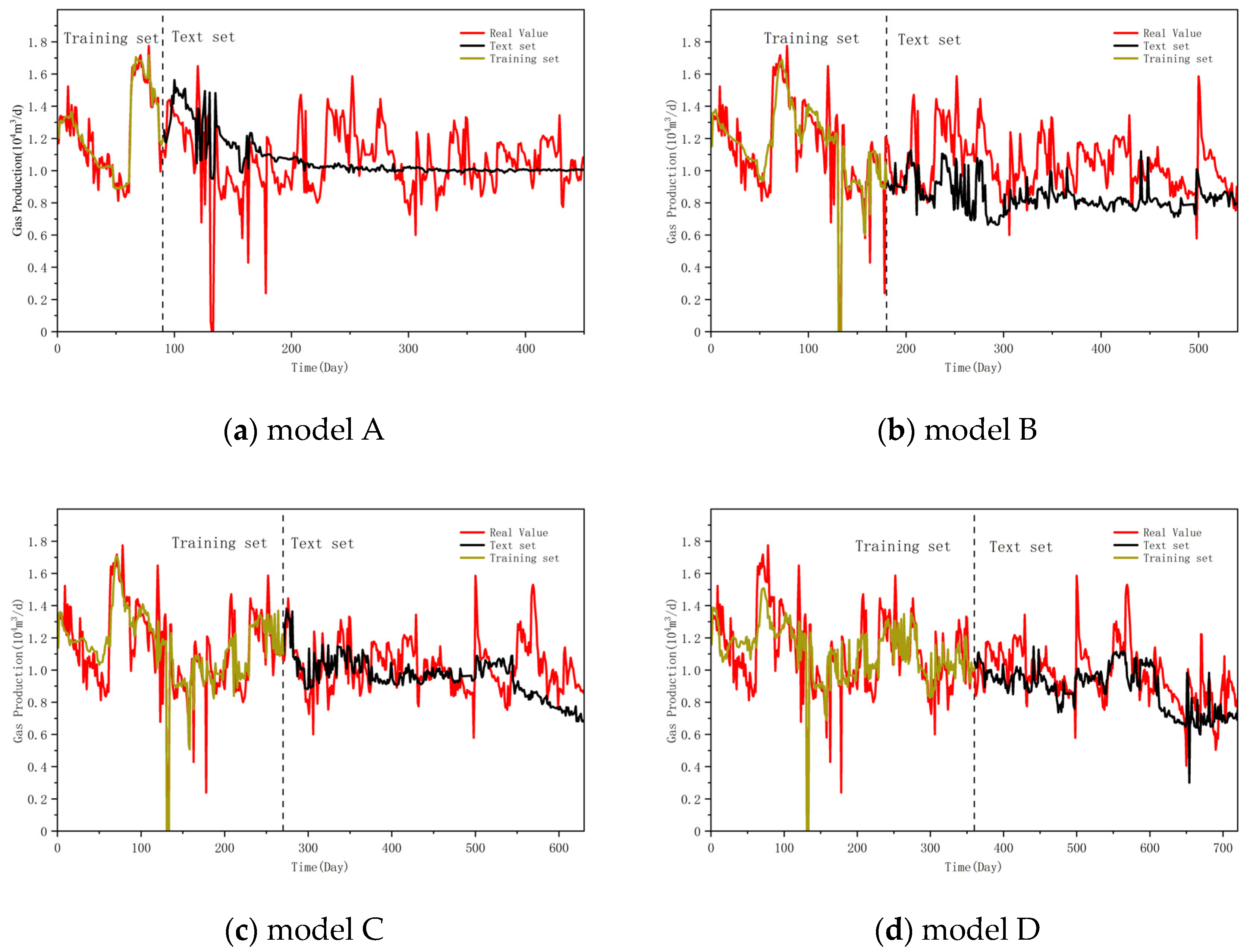
Taking well M1-46 as an example, the prediction performance of the four models is shown in Figure 12. Model D has the most accurate gas production prediction, followed by models B and C, and model A can only predict the changing trend of gas production. When Model A predicts future production, it initially performs well on the gas production data of the next 30 days. As the prediction time increases, the production change trend is smooth and shows a significant decreasing trend. This is because the model established in this paper has the physical constraint of decreasing analysis and will rely on the decreasing trend of the sample data when predicting future production. The RMSE of Model D (360 days) decreased by 24.1% to 29.7% compared with Model A (90 days) throughout the entire period. The more verification sample data there are, the more obvious the decreasing trend becomes, and the model is more accurate in predicting future production.

Based on the above analysis results, when predicting the gas production in the next 30 days, the more sample data there are, the more obvious the decreasing trend becomes, and the model’s prediction of future output is more accurate. Therefore, when using the P-C-L-A model to dynamically optimize the production allocation of production wells, based on the production allocation strategy of “long-term historical data-driven +30-day rolling prediction”, the gas production in the next 30 days is predicted with as many historical data as possible as sample data, and the production data are updated every 30 days.

5.2.2. Comparison of Different Well Shutdown Time Models

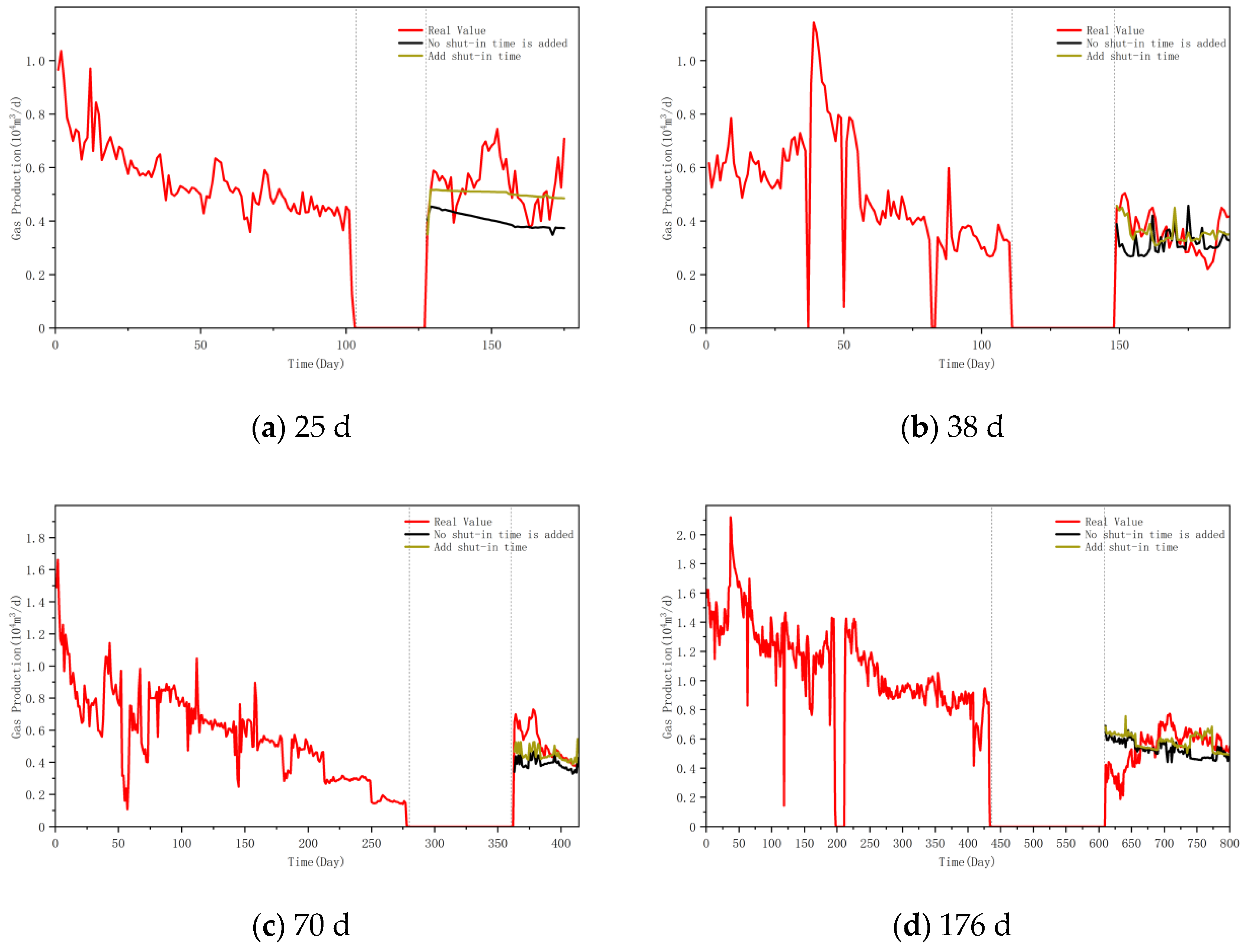
To verify the impact of well shutdown time on model performance, four gas well production data segments with different well shutdown durations (25 days, 38 days, 70 days, and 176 days) were selected to test the influence of well shutdown time on model performance and daily gas production, whether it was added or not.

It can be seen from Figure 13 that, without adding the time variable of well closure, the predicted change trend of production after well opening is more in line with the production data before well closure. After adding the well shutdown time variable, during the model training process, the pressure recovery during the short period of well shutdown time will be taken into account based on the casing pressure and tubing pressure in the characteristic parameters.

The root mean square error distribution of the Influence of well shutdown time on prediction performance was compared with and without it (Figure 14). The results show that under the four well shutdown durations, the prediction errors after adding the well shutdown time variable are significantly lower than those without adding this variable. The maximum reduction in RMSE was 41.2% (after 25 days of well closure), and the minimum was 4.1% (after 176 days of well closure). Adding the variable of well closure time led to an average reduction of approximately 24.2% in the predicted RMSE. Adding the well closure time variable can capture the key impact of well closure pressure recovery on the initial production after well opening, effectively improving the accuracy of the model in predicting the production after well opening. Therefore, the model proposed in this paper, by incorporating the factor of well shutdown time, can be more accurately applied to the production capacity prediction throughout the entire life cycle of gas wells.

5.2.3. Optimal Production Allocation for Typical Wells

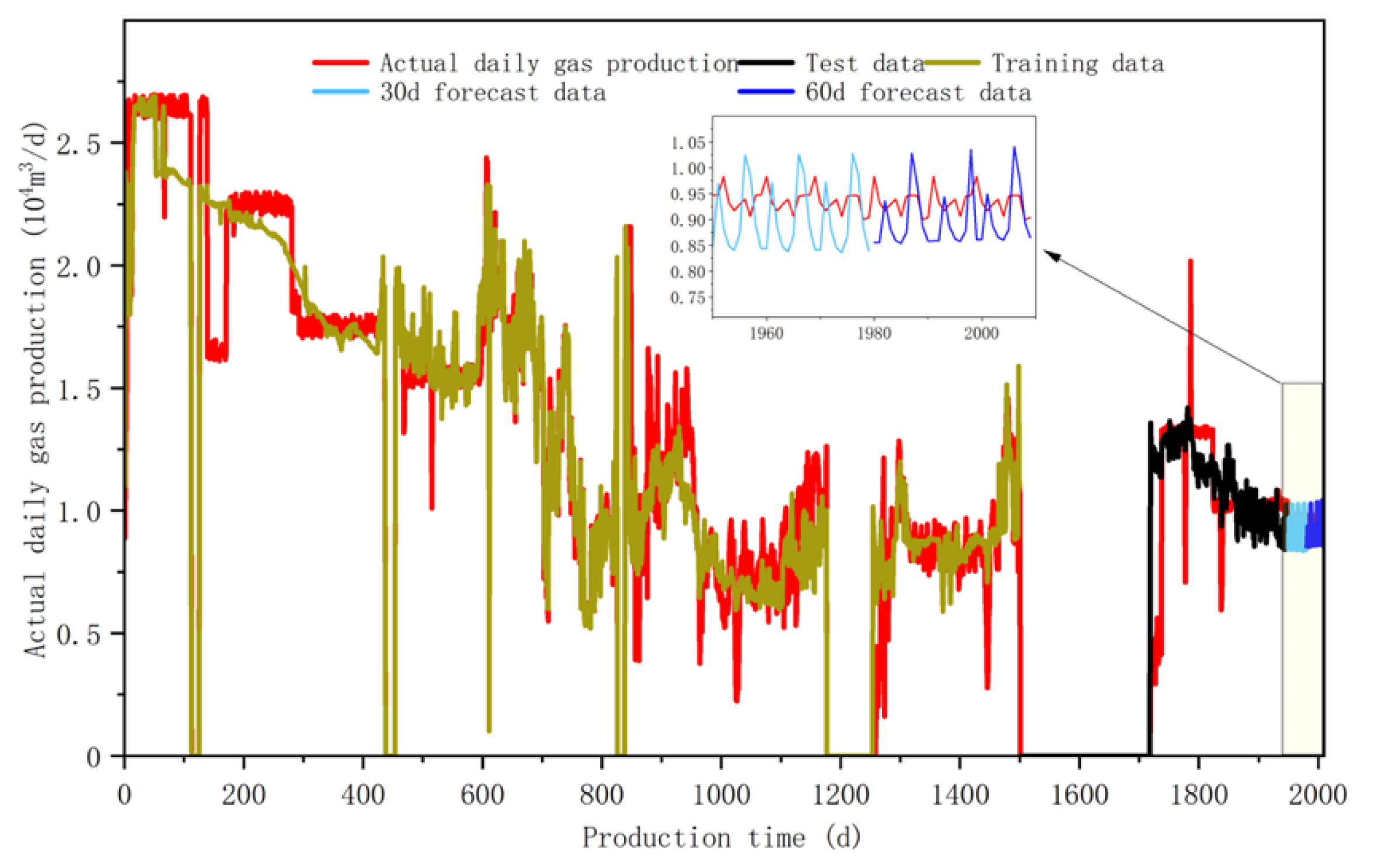
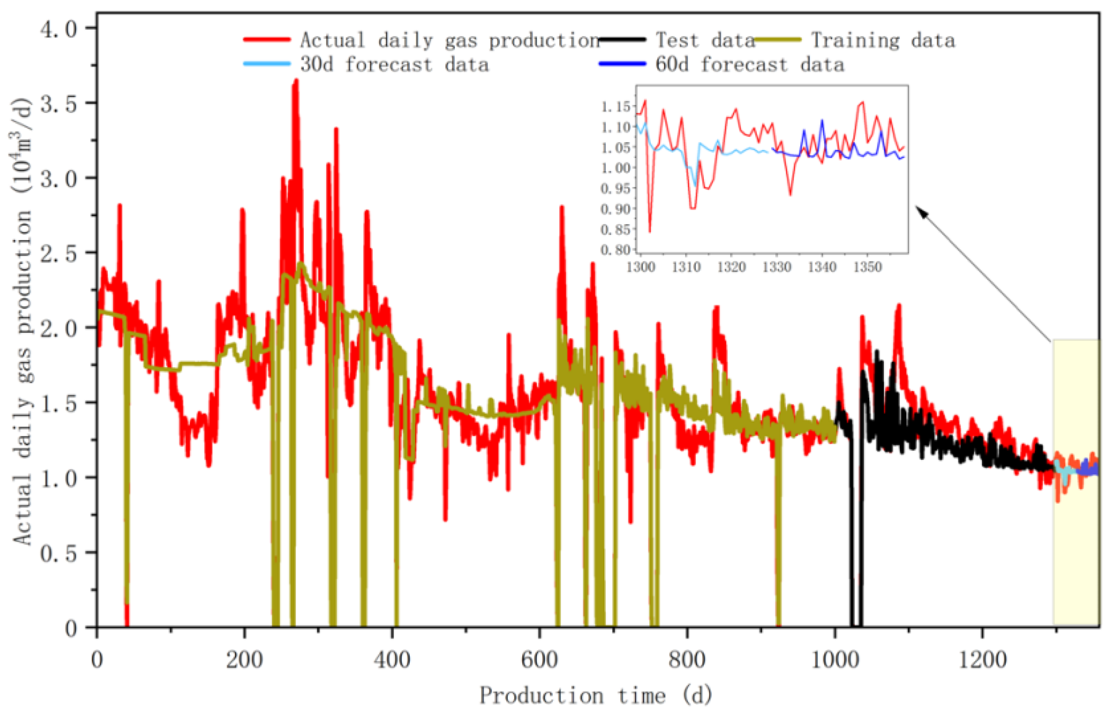
Two production wells, M10-51 and M16-5, were selected as typical wells in the study area to predict the output for the next 30 days.

(1)

Well M10-51

The average absolute error of the training set for this well is 0.1155 × 10⁴ m³ and the root mean square error is 0.1968 × 10⁴ m³. The average absolute error of the test set is 0.0759 × 10⁴ m³ and the root mean square error is 0.1818 × 10⁴ m³. The performance parameters of the model training show good results. It is predicted that the average daily gas production in the next 30 days will be 0.89 × 10⁴ m³. It is predicted that the average daily gas production over the next 60 days will be 0.89 × 10⁴ m³. It is recommended to adjust the basic production allocation to 0.90 × 10⁴ m³/d (Figure 15). By tracking the production dynamics of well M10-51, it is shown that the actual average daily gas production over the next 30 days is 0.93 × 10⁴ m³, and the machine learning dynamic production allocation results are reasonable.

(2)

Well M16-5

The average absolute error of the training set for this well is 0.1914 × 10⁴ m³ and the root mean square error is 0.2727 × 10⁴ m³. The average absolute error of the test set is 0.1379 × 10⁴ m³ and the root mean square error is 0.1921 × 10⁴ m³. Due to the large variation in the initial production output of this well, local errors are amplified during model training. After production stabilizes, the model’s trainability gradually stabilizes. It is predicted that the average daily gas production over the next 30 days will be 1.02 × 10⁴ m³, and the average daily gas production over the next 60 days will be 1.02 × 10⁴ m³. It is recommended to adjust the basic production allocation to 1 × 10⁴ m³/d (Figure 16). By tracking the production dynamics of well M16-5, it is shown that the actual average daily gas production over the next 30 days is 1.05 × 10⁴ m³, and the machine learning dynamic production allocation results are more reasonable.

6. Conclusions

(1)

This paper proposes a dual-driven model combining physical constraints and data. Its mean absolute error is 0.0985 × 10⁴ m³, and the root mean square error is 0.1417 × 10⁴ m³, which is more accurate than traditional machine learning methods.

(2)

The model integrates the local feature capture capability of CNN, the temporal dependence modeling of LSTM, and the key state focusing function of the attention mechanism to construct a multi-level feature learning system. It embeds the decline law of gas wells into the loss function to realize the joint drive of physical constraints and data of the decline curve. Ablation experiments show that each module of the model contributes to performance improvement, among which the long short-term memory neural network module has the greatest impact.

(3)

Physical parameters and weighting factors have a significant impact on the model performance. Different physical parameter constraints can reduce prediction errors from multiple dimensions, thereby improving the stability and accuracy of outputs. The optimal weighting factor can balance the influence of physical constraint loss and neural network loss in the loss function, and when it is 0.6, the physical constraints and data fitting of the model reach the best balance.

(4)

The strategy of “initial static similar production allocation +30-day historical data-driven rolling production allocation” is proposed to formulate reasonable working systems in stages and realize dynamic production optimization throughout the whole life cycle of gas wells. Based on data symmetry, the initial production allocation of similar wells was used to guide the rational production allocation of target wells. Taking 10 wells in the study area as examples, the average relative error of the initial production allocation was 7.21%. Based on the established P-C-L-A model, dynamic production allocation is carried out for stable production wells. The comparison shows that the longer the model prediction time, the lower the accuracy. The prediction of daily gas production in the next 30 days is relatively accurate, with an average root mean square error of 0.1618 × 10⁴ m³. Moreover, the model in this paper can take into account the impact of well shutdowns on production volume and is applicable to capacity prediction throughout the entire life cycle.